the Creative Commons Attribution 4.0 License.
the Creative Commons Attribution 4.0 License.
 | 19 Dec 2023
Modeling and evaluating the effects of irrigation on land–atmosphere interaction in southwestern Europe with the regional climate model REMO2020–iMOVE using a newly developed parameterization
Christina Asmus
Peter Hoffmann
Joni-Pekka Pietikäinen
Jürgen Böhner
Diana Rechid
Irrigation is a crucial land use practice to adapt agriculture to unsuitable climate and soil conditions. Aiming to improve the growth of plants, irrigation modifies the soil condition, which causes atmospheric effects and feedbacks through land–atmosphere interaction. These effects can be quantified with numerical climate models, as has been done in various studies. It could be shown that irrigation effects, such as air temperature reduction and humidity increase, are well understood and should not be neglected on local and regional scales. However, there is a lack of studies including the role of vegetation in the altered land–atmosphere interaction. With the increasing resolution of numerical climate models, these detailed processes have a chance to be better resolved and studied. This study aims to analyze the effects of irrigation on land–atmosphere interaction, including the effects and feedbacks of vegetation. We developed a new parameterization for irrigation, implemented it into the REgional climate MOdel (REMO2020), and coupled it with the interactive MOsaic-based VEgetation module (iMOVE). Following this new approach of a separate irrigated fraction, the parameterization is suitable as a subgrid parameterization for high-resolution studies and resolves irrigation effects on land, atmosphere, and vegetation. Further, the parameterization is designed with three different water application schemes in order to analyze different parameterization approaches and their influence on the representation of irrigation effects. We apply the irrigation parameterization for southwestern Europe including the Mediterranean region at a 0.11∘ horizontal resolution for hot extremes. The simulation results are evaluated in terms of the consistency of physical processes. We found direct effects of irrigation, like a changed surface energy balance with increased latent and decreased sensible heat fluxes, and a surface temperature reduction of more than −4 K as a mean during the growing season. Further, vegetation reacts to irrigation with direct effects, such as reduced water stress, but also with feedbacks, such as a delayed growing season caused by the reduction of the near-surface temperature. Furthermore, the results were compared to observational data, showing a significant bias reduction in the 2 m mean temperature when using the irrigation parameterization.
- Article
(12277 KB) - Full-text XML
- BibTeX
- EndNote


Land use and land use practices are anthropogenic forcings that were shown to influence regional climate. They can be defined as the modification of the land surface through anthropogenic changes in land cover types or land use practices that alter the land surface within one land cover type (Luyssaert et al., 2014). Through land–atmosphere interactions, changes in the land conditions can affect the climate and cause feedback mechanisms, especially in the near-surface atmosphere levels (Jia et al., 2019). Luyssaert et al. (2014) pointed out that under specific circumstances the effects of land use practices reach the same magnitude as land use and land cover change effects and should therefore not be neglected in climate studies. We find different land use practices in agriculture such as tillage, fertilization, and irrigation. Irrigation is the land use practice that has the strongest impact on the climate (Kueppers et al., 2007; Lobell et al., 2009; Sacks et al., 2009). Further, irrigation is a common land use practice in agriculture to adapt to unsuitable climatic conditions. Using numerical models, irrigation effects are studied on different scales, with different parameterizations, and for different regions. An overview can be found in Valmassoi and Keller (2022), who collected different irrigation modeling studies and identified the different aspects of irrigation parameterizations as sources of uncertainties for irrigation effects on the climate.
Global-scale irrigation studies show different developments of irrigation effects in different regions in the world (Thiery et al., 2017, 2020; Sacks et al., 2009; Lobell et al., 2009; Puma and Cook, 2010; de Vrese and Hagemann, 2018). All studies found near-surface and surface temperature reduction. Compared to observational data, using irrigation in the model of Lobell et al. (2009) could eliminate the warm and dry bias of CLM. de Vrese and Hagemann (2018) showed that irrigation has remote effects more than 100 km of distance from the irrigated area. Further, multiple studies showed that irrigation effects are more pronounced on local and regional scales (Sacks et al., 2009; Kueppers et al., 2007; Valmassoi et al., 2020c). In particular, high-resolution studies on a regional scale require an accurate representation of the land surface and soil processes to represent local and regional climatic patterns (Hagemann et al., 1999). For example, Saeed et al. (2009) showed the irrigation effects on the summer monsoon in India, which is weaker due to a smaller land–sea–temperature gradient. Also, Tuinenburg et al. (2014) studied irrigation effects in India and found a shift in the precipitation pattern through the additional moisture in the atmosphere. Valmassoi et al. (2020a) studied irrigation effects in the Po Valley on a convection-permitting scale and found an increase in precipitation in irrigated areas. Like Thiery et al. (2020) on a global scale, Kueppers et al. (2007) pointed out the potential of irrigation to mask the warming effects of greenhouse gases on a regional scale for a study in California. Further, Kueppers et al. (2007) showed that irrigation effects follow a seasonality. During the growing season, the effects are most pronounced, and for dry periods the effects are stronger than for wet periods. Thiery et al. (2020) and Jia et al. (2019) point out that the near-surface temperature reduction through irrigation decreases the probability of hot extremes. With these characteristics, irrigation becomes a potential adaptation measure to climate extremes, not only for water stress that plants experience during droughts, but in addition, it can be implemented to reduce the intensity of heat waves.
The simulated effects of irrigation on the land–atmosphere interaction depend, on one hand, on the amount of irrigation, as pointed out by Valmassoi et al. (2020c), and on the other hand on the design of the parameterization itself. The irrigation amount is driven by the soil hydrology of the model. Multiple models represent the soil hydrology using a layered scheme and prescribe observed irrigation amounts (Valmassoi et al., 2020c; Puma and Cook, 2010; Ozdogan et al., 2010; Yao et al., 2022). For models using a bucket scheme (Boucher et al., 2004; de Vrese and Hagemann, 2018), observed irrigation values might not fit due to the deep bucket. Therefore, the irrigation parameterizations are designed with thresholds based on specific model-internal physical values, e.g., values of the maximum water-holding capacity of soil, field capacity, leaf area index (LAI), or photosynthesis rates, to determine the irrigation amount or the irrigation start and end. However, using such a model-internal physical threshold rather than a prescribed irrigation amount often leads to an overestimation of the effects (Kueppers et al., 2007). Therefore, Thiery et al. (2017) added a water limit for the available irrigation amount to reach realistic values, and Leng et al. (2017) added a water source and closed the hydrological cycle. For representing irrigation in a climate model, it is recommended to have a separate soil column for irrigation (Lobell et al., 2009; Ozdogan et al., 2010; Thiery et al., 2017) and represent irrigated areas on a subgrid scale. Another aspect of representing irrigation in a climate model is the irrigation method. Irrigation methods differ in their water application. Mostly, irrigation is represented as an increase in soil moisture, neglecting canopy interactions (Sacks et al., 2009; Lobell et al., 2009; Ozdogan et al., 2010; Thiery et al., 2017; de Vrese and Hagemann, 2018). Newer studies consider canopy effects which are caused by, e.g., sprinkler irrigation (Valmassoi et al., 2020c; Leng et al., 2015; Yao et al., 2022). However, on a regional scale, the differences in the irrigation effects between different irrigation methods remain small and can be neglected (Valmassoi et al., 2020c).
For most methods, irrigation affects the land surface, altering the exchange processes through land–atmosphere interaction. At high resolution, a more detailed representation of the land surface and its processes is possible. An important driver of these land processes, such as the soil, the land surface, and the atmosphere, is vegetation, which is also affected by irrigation. However, there is a lack of high-resolution climate studies which include the irrigation effects on vegetation and its feedback on the atmosphere, soil, and surface. This study aims to represent irrigation effects in the model system REMO2020–iMOVE which represents land, atmosphere, and vegetation processes interactively. Whereas Saeed et al. (2009) analyzed large-scale irrigation effects with REMO2009, this study aims to provide a detailed representation of irrigation aspects and conducts high-resolution experiments. Thus, we implement a new irrigated fraction and represent irrigation on a subgrid scale. Our model region is southwestern Europe with a focus on one of the most intensely irrigated areas in Europe, the Po Valley. After we describe the model and the data that we used for this study in Sect. 2, we introduce our new irrigation parameterization (Sect. 3). In Sect. 4 we apply the new irrigation parameterization and evaluate it with the consistency of physical processes as well as with the comparison of observational data. We point out some limitations of our parameterization in Sect. 5 and give concluding remarks in Sect. 6.
2.1 The model REMO2020–iMOVE
For this study, the regional climate model REMO2020 was used. REMO is developed as a hydrostatic atmospheric circulation model based on the primitive equations of atmospheric motion at the Max Planck Institute for Meteorology, Hamburg, Germany (Jacob, 1997, 2001). It combines parts of the Europa Model (EM) of the German Weather Service (Majewski, 1991) and the physical parameterizations of ECHAM4 (Roeckner et al., 1996). With time, REMO was further developed and received additional features such as dynamic vegetation cover (Rechid and Jacob, 2006), glaciers (Kotlarski, 2007), lakes (Pietikäinen et al., 2018), a non-hydrostatic extension to the hydrostatic core (Goettel, 2009), and an interactive mosaic-based vegetation module (iMOVE) (Wilhelm et al., 2014). For this study, in particular, the land surface parameterizations are of interest.
The surface of one model grid box in REMO2020 is represented with the tile approach in which the subgrid fractions land, water (representing sea and lakes), and sea ice are introduced (Semmler, 2002). Using the lake module FLake (Pietikäinen et al., 2018), a separate lake subgrid fraction is added. In total, the fractions sum up to 100 % of the surface of a model grid box. Whereas the land fraction is constant, the sea ice fraction can vary, thereby changing the water fraction. For each fraction turbulent surface fluxes and radiation fluxes are calculated and averaged at the lowest atmospheric level using weighted means with respect to the fraction area of the model grid cell. Using the bulk transfer relations with transfer coefficients from the Monin–Obukhov similarity theory with a higher-order closure scheme, the turbulent fluxes of momentum and heat are calculated (Kotlarski, 2007). The exchange processes between the atmosphere and surface are determined by the vegetation coverage. Since the vegetation physiology depends strongly on seasonal cycles, the variations are included for the vegetation fraction, the LAI, and the background albedo (Rechid and Jacob, 2006). To improve the vegetation representation and its effects on the atmosphere, the iMOVE modules of REMO2009–iMOVE (Wilhelm et al., 2014) are implemented into REMO2020. Multiple elements of iMOVE are based on the dynamic land surface scheme JSBACH (Raddatz et al., 2007; Wilhelm et al., 2014). It represents the land cover with tiles of plant functional types (PFTs) using the Holdridge ecosystem classification scheme (Wilhelm et al., 2014). For this experiment, the definition and distribution of PFTs are based on the land cover maps of the European Space Agency Climate Change Initiative (ESA-CCI) (Reinhart et al., 2022; Hoffmann et al., 2023). The PFTs interact dynamically with the atmosphere and the soil, leading to varying phenology. Here, soil moisture and air temperature are important driving factors (Wilhelm et al., 2014). Furthermore, in REMO2020–iMOVE soil moisture determines the soil albedo following the findings of Peterson et al. (1979) and model adjustments of Wilhelm et al. (2014). As a result, the soil albedo is represented with a negative exponential relationship with the soil moisture.
The heat budget of the soil is represented with a five-layer scheme. The heat transfer is calculated with diffusion equations for five discrete layers. For solving the equations, it is assumed that the heat flux is zero at the lowest boundary. The heat transfer between the layers is mainly driven by the heat conductivity and heat capacity of the soil type, which vary with soil moisture. The soil hydrology consists of three water storage reservoirs: soil, skin reservoir (vegetation), and snow, for which budget equations are solved. The reservoirs are altered by precipitation, interception, dew, evapotranspiration, snowmelt, runoff, infiltration, and drainage (Kotlarski, 2007). Precipitation is split by the improved Arno scheme (Dümenil and Todini, 1992) into surface runoff and infiltration considering subgrid-scale heterogeneous field capacities of the land surface within one grid cell (Hagemann, 2002). The field capacity in REMO is at the level of the maximum water-holding capacity (wsmx), which is based on the global dataset of land surface parameters (LSPs) by Hagemann et al. (1999). Once the soil moisture reaches wsmx, runoff occurs. Infiltration fills up the soil moisture reservoir, which is represented as a simple bucket scheme with subsurface drainage. The drainage is led by the ratio of the soil moisture and wsmx. Drainage occurs for soil moisture larger than 5 % of wsmx. Between 5 % and 90 % of wsmx, drainage is slow. If the soil moisture is larger than 90 % of wsmx, the drainage is fast (Kotlarski, 2007).
Water can leave the soil moisture reservoir through evapotranspiration depending on vegetation characteristics and atmospheric conditions. For bare soil, evaporation takes place from the upper 10 cm. Subsurface water leaves the soil moisture reservoir only through transpiration by vegetation or drainage. At the surface or soil, there are no lateral flows of water within REMO2020 (Wilhelm et al., 2014).
2.2 Irrigation dataset
For an estimation of the spatial distribution of irrigated areas, the Global Map of Irrigated Areas Version 5 (GMIA5) by Siebert et al. (2013a) is used. The GMIA5 describes the area equipped for irrigation as well as the area actually irrigated on a resolution of 5 arcmin (0.083333 decimal degrees). It was developed at the Johann Wolfgang Goethe University, Frankfurt (Main), Germany, by Doell and Siebert (1999). Through cooperation with the Rheinische Friedrich-Wilhelms-Universität, Bonn, Germany, and the Land and Water Division of the FAO, GMIA is constantly improved and updated. The dataset is mainly based on AQUASTAT, the FAO's information system on water and agriculture. The data are collected from national and subnational water resources and irrigation plans, statistics, yearbooks, and FAO technical reports. This information is combined with geospatial information on the position and extent of the irrigated area. The statistical data refer to the years 2000 to 2008, with the reference year depending on the country. The quality of GMIA5 was assessed by the density of subnational irrigation statistics used and by the density of the available geospatial records on the position and extent of irrigated areas (Siebert et al., 2013b).
For our study, we chose the data on the “area equipped for irrigation” of the GMIA5 due to better quality (Siebert et al., 2013b) as well as due to our study's purpose of showing maximal possible irrigation effects.
2.3 Observation data for evaluation
The Italian Institute for Environmental Protection and Research (ISPRA) established a database for meteorological observation data for Italy named SCIA (Italian: Sistema nazionale per la raccolta, l'elaborazione e la diffusione di dati Climatologici di Interesse Ambiental). SCIA works as a framework of the national environmental information system and combines data from national and regional networks, agro-meteorological stations (UCEA-RAN), hydro-meteorological stations, and tide gauge networks. The data are updated once per year and undergo a quality check. Climate indicators are available for different timescales such as means of 10 d, months, or years (Desiato et al., 2011) and are freely available on the SCIA website (http://www.scia.isprambiente.it, last access: 8 December 2023). For this study, the monthly means of the daily mean, maximum, and minimum 2 m temperature for the year 2017 are used.
3.1 Implementation of a new irrigated land subfraction and a new PFT into REMO2020–iMOVE
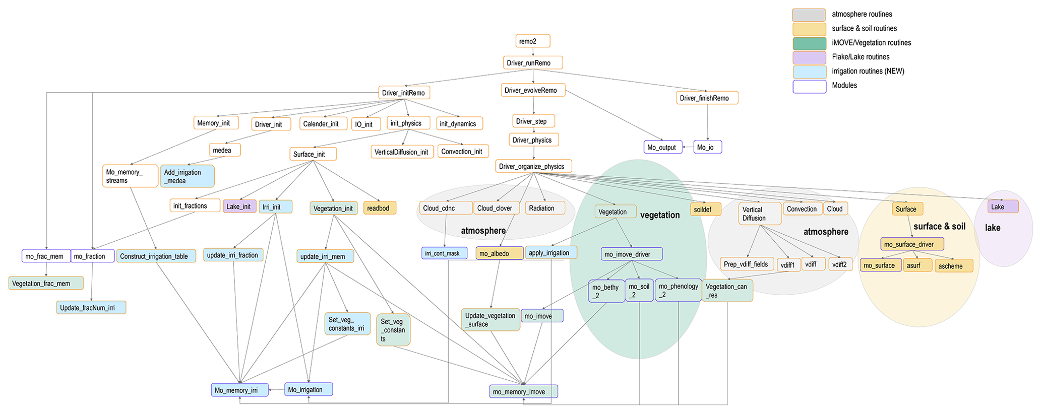
In REMO2020–iMOVE, soil processes are defined for land fractions (Kotlarski, 2007). Irrigation influences soil and surface directly and is a new local process to implement into REMO2020–iMOVE. Since it affects the land fraction, we implement a new irrigated land fraction based on the “area equipped for irrigation” from the GMIA5 (Sect. 2.2). Before using it in REMO–iMOVE, GMIA5 has to be adapted to the desired resolution and geographic projection. The new irrigated land fraction in REMO2020–iMOVE is a new land fraction that can be understood as a subfraction of the land fraction (Fig. 1). All soil, surface, and vegetation processes are calculated for both land fractions, except for irrigation, which is applied exclusively to the irrigated land fraction.
As land cover, we implement a new PFT named “irrigated cropland” on the irrigated land fraction. The properties of irrigated cropland are based on the properties of the “cropland” PFT of the non-irrigated land fraction. REMO2020–iMOVE is able to distinguish between the photosynthesis path of cropland PFTs (C3 or C4); however, it does not distinguish between different crop types. In our case irrigated cropland is the only irrigated PFT and therefore the only PFT on the irrigated land fraction. With the separation into an irrigated and non-irrigated land fraction and the new PFT, we ensure that the irrigation process is only applied to areas that are truly irrigated. Having a separate irrigated land fraction gives a detailed representation of the heterogeneity of the surface and irrigated areas, which is an advantage for high-resolution and small-scale irrigation studies such as on the European continent where irrigated areas are rather scattered.
The implementation of the new irrigated land fraction is done during the model initialization. The irrigation module, which accounts for a check of irrigation requirements and water application, is called every time step exclusively for the irrigated land fraction. These irrigation processes are carried out after the hydrological processes of the soil from the previous time step (t−1). In this way, the irrigation processes are applied to the soil hydrology inherited from t−1. After the irrigation processes, the vegetation processes start, which are strongly influenced by the moisture content in the soil and in the atmosphere of the same time step (t) (Fig. A1).
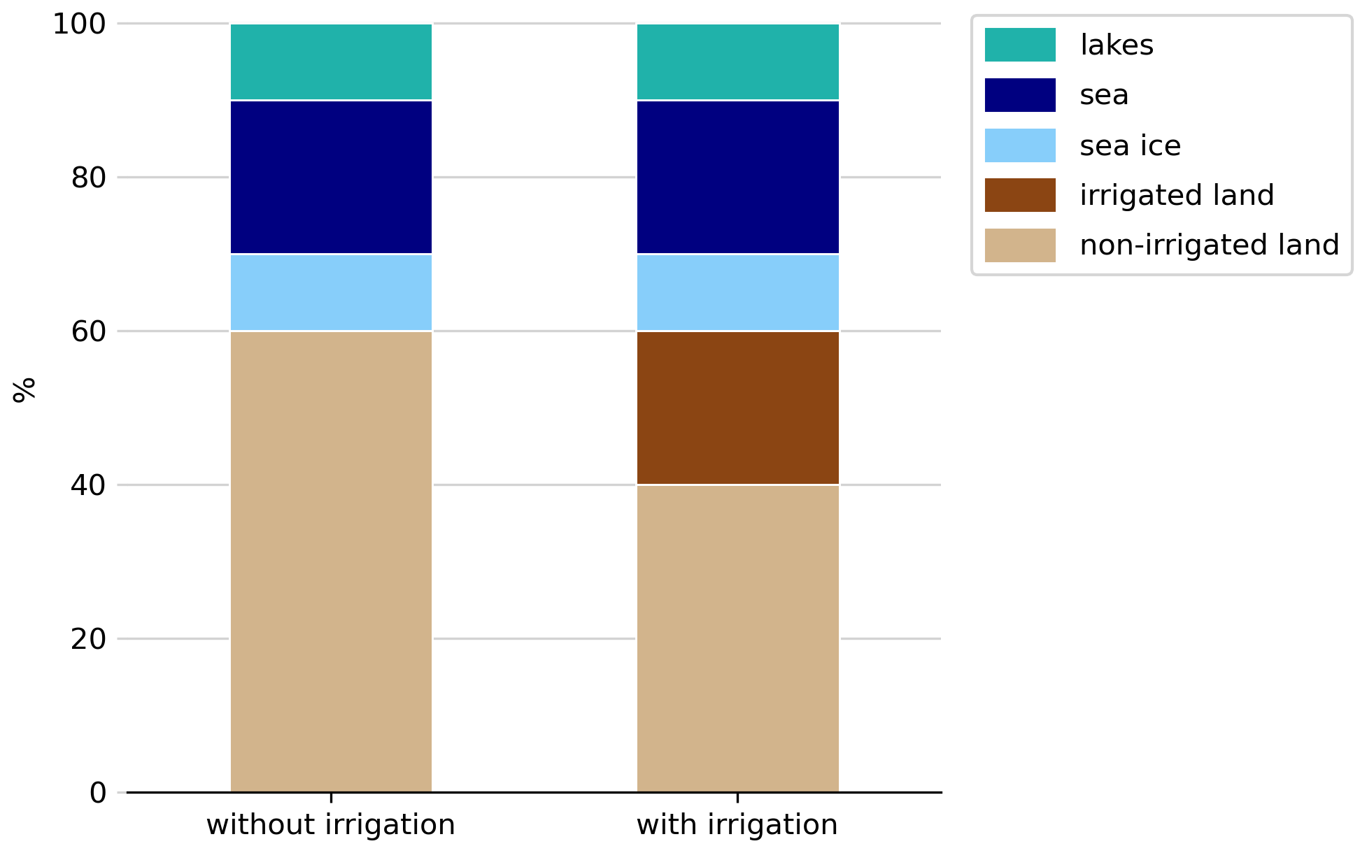
Figure 1Fractions of one example model grid cell in REMO2020–iMOVE + FLake with and without irrigation.
3.2 Irrigation module and its different water application schemes
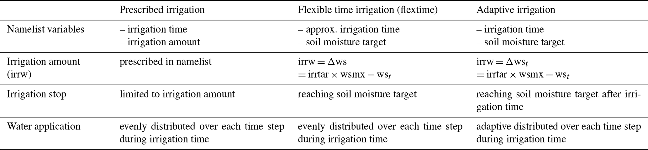
We implemented the new irrigation module into REMO2020–iMOVE, which can be turned on and off. The irrigation module determines where, when, and how irrigation will be applied. Irrigation is exclusively applied to the irrigated fraction (Sect. 3.1), which defines the area equipped for irrigation from Siebert et al. (2013a) (Sect. 2.2). Using an adjustable threshold (irrthr) on the soil moisture, the irrigation module determines the grid cells with irrigation requirements and creates a daily irrigation mask at 7:00 LT as the starting time for irrigation in our parameterization following Valmassoi et al. (2020c). This determination is carried out during the growing season because only then do plants require irrigation. The growing season depends on the location and a growing degree threshold (Wilhelm et al., 2014). Upon fulfilling the requirements for irrigation (Fig. 2), the water application starts. For parameterizing channel irrigation, the water is added directly to the soil and increases the soil moisture. Here, we assume an infinite water supply. The water application and the irrigation amount strongly depend on the soil hydrology parameterization of the climate model, as well as on the intention of being close to reality. Therefore, we implemented three different water application schemes, which can be used for different purposes (Table 1).
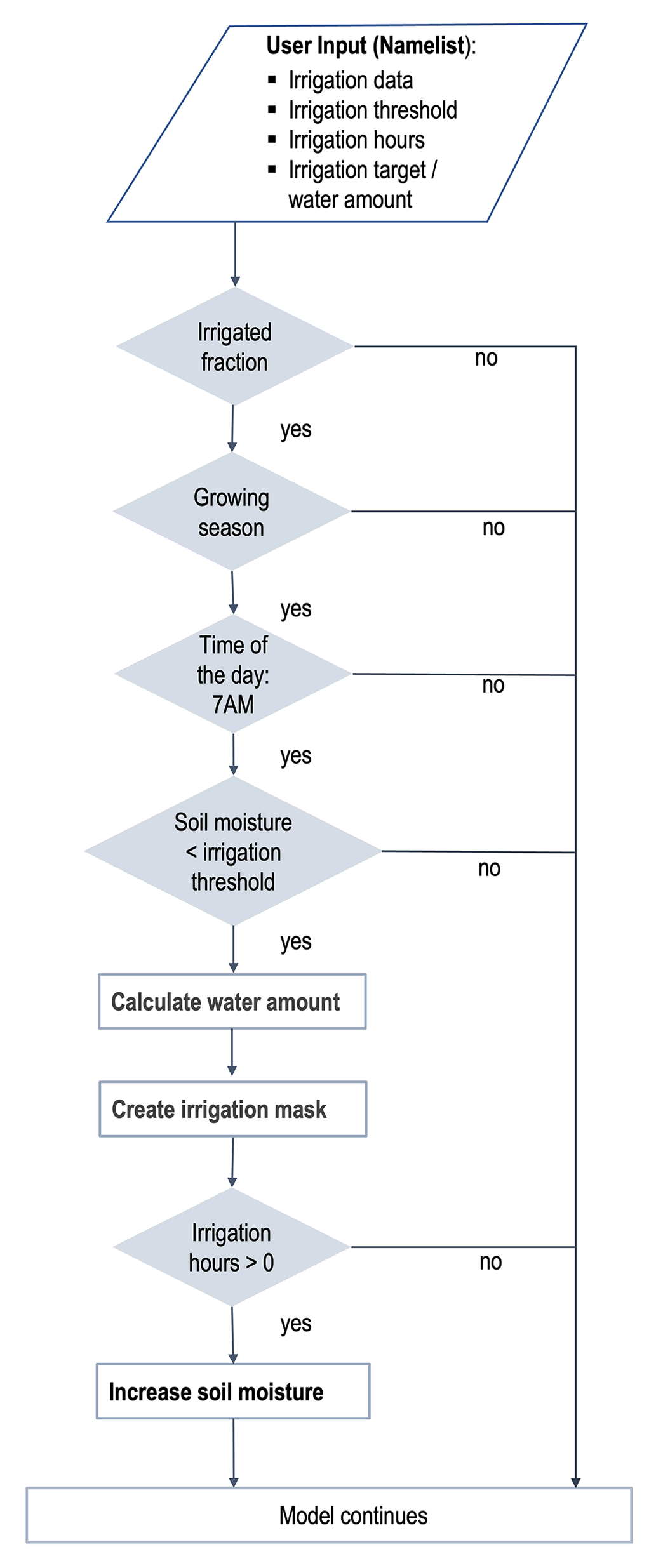
The “prescribed irrigation” scheme applies a prescribed amount of water within a prescribed time. The prescribed water amount will be equally distributed over each time step during the irrigation time. The water amount can be based on observed irrigation values, but also extreme situations: a limited water supply or a huge water supply can be simulated. However, having a simple soil hydrology parameterization, such as the bucket scheme in REMO2020–iMOVE, suitable values for the prescribed water amount might differ from observed irrigation amount values, leading to a necessary adjustment to reach realistic soil moisture conditions in the model. The prescribed water amount is a universal value, which will be added to the irrigated fraction in all model grid cells that fulfill the irrigation requirements (Fig. 2). Further, the water amount in the model does not depend on the crop type, since REMO–iMOVE does not distinguish between different crop types.
The “flexible time irrigation (flextime)” is based on a prescribed soil moisture target and open irrigation time. For each grid cell, the water amount is calculated that is necessary to reach the soil moisture target. Again, the water amount is equally distributed over each time step within the prescribed time. Once the soil moisture target is reached, the water application stops regardless of the irrigation time. For this approach, a soil moisture target has to be chosen in relation to wsmx of the soil.
The “adaptive irrigation” is also based on a prescribed soil moisture target and a prescribed, limited irrigation time. Again, for each grid cell, the water amount is calculated that is necessary to reach the soil moisture target. The water amount added every time step follows a relaxation approach (Eq. 1) which simulates the increase in soil moisture during the time steps of irrigation and simultaneously considers the changes in soil moisture not related to irrigation. Further, our relaxation approach takes into account the number of irrigation time steps remaining. Using this approach the soil moisture increases until the irrigation target is exactly reached during the prescribed irrigation time:
where ws is soil moisture, irrtar is irrigation target, wsmx is maximum water-holding capacity, nirr is the number of remaining irrigation time steps, and t is the time step.
Table 1Properties of the different water application schemes in REMO2020–iMOVE.
4.1 Experiment setup
We employ REMO2020–iMOVE for our model domain covering southwestern (SW) Europe and the Mediterranean region, including some of the most intensely irrigated areas such as the Po Valley and the Ebro Basin (Fig. 3). In 2017, SW Europe experienced exceptionally high temperatures, starting in June and reaching a heat wave in early August (Sect. 4.3). This is the period we chose for our simulation because, first, irrigation is most important for agriculture during hot periods, and second, the effects of irrigation are most pronounced (Kueppers et al., 2007).
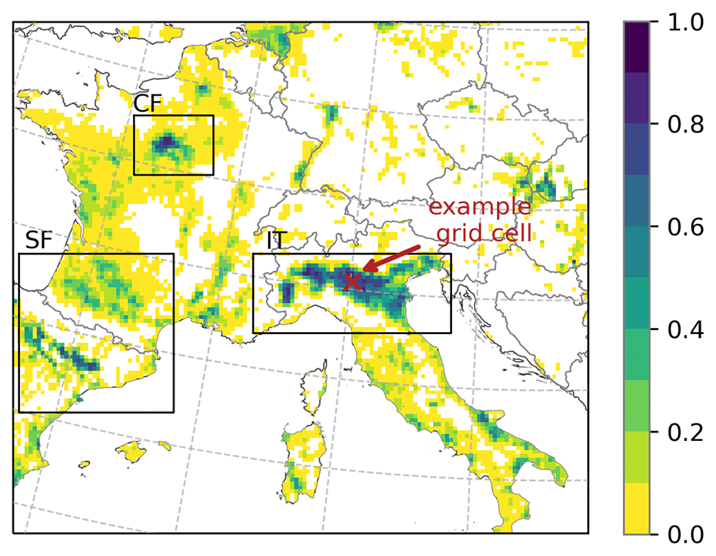
Figure 3Model domain grid cells with the fraction of irrigated areas interpolated from area equipped for irrigation in Siebert et al. (2013a) and the analysis regions in Italy (IT), northern Spain and southern France (SF), and central France (CF). The example grid cell of Sect. 4.2 is pointed out.
We conduct three 1-month simulations to test the different water application schemes (T1–T3, Table 2) for June 2017. Based on these short tests, we decide on one water application scheme to conduct a 1-year simulation (S1) and analyze the effects of irrigation in the course of the year 2017. Simulation S0 is our baseline experiment and does not apply irrigation. All our simulations use a rotated grid with the rotated North Pole at 39.25∘ N, 162∘ W and have a horizontal resolution of 0.11∘. We use ERA5 on 50 vertical levels as boundary data and set the time step to 60 s. S0 and S1 start from 1 January 2017. We initialized S0 and S1 with ERA5 (Table 2), except for the soil conditions. Since soil conditions have a long spin-up time in regional climate models (RCMs), we initialize the soil variables with a previous long-term (>10 years) REMO simulation to get the soil variables in an equilibrium state. This method is also known as a “warm start” (Pietikäinen et al., 2018). The test simulations are started as a restart from our baseline experiment S0 from 1 June 2017. Table 2 summarizes the settings for the different test simulations T1 to T3, as well as for the 1-year simulations S0 and S1.
T1, T2, and T3 test the water application schemes prescribed, flexible time (flextime), and adaptive to estimate their effect on the development of irrigation effects. For all three test simulations, the irrigation threshold for the soil moisture is set to 0.75 of wsmx. For the model, this threshold is important because, from 0.75 of wsmx, the vegetation processes have optimal conditions to develop.
T1 uses a prescribed irrigation amount of 150 mm d−1 which is evenly distributed over the irrigation time in all grid cells with irrigation requirements. We selected 150 mm d−1 as the irrigation amount from experience using the bucket scheme as soil hydrology (Sect. 3.2). Following Bjorneberg (2013) and Zucaro (2014) channel irrigation is performed for up to 24 h depending on the channel width and length; we chose 10 h irrigation time for our experiment. With the irrigation start time at 7:00 LT (Sect. 3.2), irrigation is applied during daytime in our experiment. T2 tests the water application scheme with flexible time. This water application scheme is driven by the difference between the soil moisture at irrigation start at 7:00 LT and the irrigation target. We set the irrigation target to the maximum water-holding capacity. T3 tests the adaptive water application scheme. As in T2, the irrigation target is set to the maximum. The irrigation time is set to 10 h as in T1. Since the test simulations are started as restarts from S0, the irrigation module detects grid cells with irrigation requirements from 1 June 2017.
Table 2Simulation setup for the different water application scheme tests and the 1-year simulation.
* With soil conditions in equilibrium state from previous REMO simulation.
After testing the irrigation parameterization with its different water application schemes, our experiment aims to investigate irrigation effects on multiple variables and processes in the model system REMO2020–iMOVE and to check their physical consistency over the course of 1 year. We quantify the irrigation effect by the difference between one simulation with the irrigation parameterization turned on (S1) and our baseline simulation with the irrigation parameterization turned off (S0). In S1 the irrigation process starts with the growing season of crops in the model domain. It only turns off once the crops are harvested. In the course of the year, we analyze delayed irrigation effects and how they affect hot extremes. S1 applies the adaptive water application scheme with the irrigation threshold and the irrigation target at wsmx, leading to the maximum irrigation effects.
4.2 Testing the different water application schemes
Figure 4 shows the irrigation process with the different water application schemes for one representative irrigated grid cell in the Po Valley (63, 85) (Fig. 3) for the first irrigation day, 1 June 2017. We use a single grid cell to analyze the development of soil moisture in detail without any averaging. The soil moisture is at 0.47 of wsmx, leading to irrigation from 7:00 LT. For the prescribed water application scheme (T1) the soil moisture increases linearly until the irrigation time is finished, in this case at 17:00 LT (Fig. 4a). During the irrigation time, the same water amount is added for every time step. In the example grid cell, it is 15 mm h−1 (Fig. 4b). At the end of irrigation, soil moisture reaches 0.87 of wsmx and stays close to this level until the end of the day (Fig. 4a).
For the simulation using the flextime water application scheme (T2) the soil moisture increases linearly until the irrigation target is reached after 301 min (Fig. 4a). As in T1, the same water amount is added to the soil moisture for each time step. However, the amount of added water is driven by the difference between the soil moisture at 7:00 LT and the irrigation target, leading to a higher added water amount per time step than in T1 (40 mm h−1, Fig. 4b).
The adaptive water application scheme causes a nonlinear increase in the soil moisture, converging to the irrigation target and reaching it in the last time step of the irrigation time (Fig. 4a), which is set to 10 h. The water application adjusts itself in each time step depending on the difference between the actual soil moisture and the irrigation target as well as on the remaining time steps with irrigation (Eq. 1). Thus, for the first irrigation time steps, when the difference is the greatest, the water amount added is the greatest at 38 mm h−1. It decreases with the following irrigation time steps (Fig. 4b).
Comparing the irrigation amount used in June (Fig. 5), the water amount added in T2 and T3 is very similar (max. 380 mm per month), which is also shown in the distribution of the irrigation water amount in Fig. 5d. The irrigation water amount added by the prescribed scheme in T1, in particular, in grid cells in the Po Valley, the Ebro Basin, and southern Italy is larger than in T2 and T3. The prescribed scheme also reaches the highest irrigation water value (max. 450 mm per month, Fig. 5d). The reason for these differences is that the prescribed water application scheme stops the irrigation in one day once the prescribed irrigation amount is finished within the prescribed irrigation time, regardless of the saturation of soil moisture. This leads to multiple irrigation requirements in June once the soil moisture drops below the irrigation threshold, turning on irrigation. Using the flexible time (T2) and the adaptive water application scheme (T3), in most grid cells only one irrigation event is necessary in June, whereas using the prescribed irrigation scheme (T1) required up to three irrigation events always adding the same prescribed irrigation amount (Fig. A2).
The overall effects of the three water application schemes as monthly mean values are similar (Figs. A3, A4). Therefore, we select only one scheme to further analyze the effects of irrigation on the regional climate. The water application scheme selected is the adaptive water application scheme, since it has multiple advantages. First, it smoothly reaches the irrigation target and takes into account the actual soil moisture of each grid cell and the remaining irrigation time steps. Second, the relaxation method is a common method in climate modeling. And third, the adaptive water application scheme is the user-friendliest scheme of the three schemes because it does not require experience values of the irrigation amount depending on the soil hydrology of the climate model.
Figure 4Irrigation process on the first irrigation day (1 June 2017) using the different water application schemes in one representative example grid cell (63, 85). Settings: irrigation threshold at 0.75 of wsmx, irrigation target at wsmx, irrigation time of 10 h. The blue shaded region is irrigation time. (a) Soil moisture as a fraction of wsmx and (b) irrigation water used.
Figure 5Irrigation water used for the different water application schemes in June 2017: (a) prescribed (T1), (b) as the difference between prescribed (T1) and flextime (T2), (c) as the difference between the prescribed (T1) and adaptive scheme (T3), and (d) the distribution of irrigation water in irrigated grid cells.
4.3 Simulated meteorological conditions during spring and summer 2017 with REMO2020–iMOVE
SW Europe and the Mediterranean region experienced dry and warm weather during spring and summer in 2017. According to E-OBS data, spring (MAM) was 1.7 ∘C warmer than the reference period 1981–2010. During summer (JJA) several heat waves occurred in SW Europe, as well as in the Balkans (Copernicus Climate Change Service, 2023). One of the first heat waves hit SW Europe in June (Sánchez-Benítez et al., 2018), in particular Spain and France. Another heat wave developed at the beginning of August 2017 in southern Europe, this time in particular in Spain, France, Italy, and the Balkans (Kew et al., 2019), causing several wildfires (Copernicus Climate Change Service, 2023).
Figure 6Simulated mean meteorological condition with REMO2020–iMOVE for (a) 2 m temperature during AMJ, (b) soil moisture during AMJ, (c) monthly mean of summed precipitation for AMJ, (d) 2 m temperature during a heat wave (3–5 August 2017), (g) mean soil moisture during a heat wave (3–5 August 2017), and (f) mean of summed precipitation during a heat wave (3–5 August 2017).
The warm and dry meteorological conditions in spring as well as the hot conditions in summer are represented in the REMO2020–iMOVE simulation in the southern part of the model domain (Figs. 6, 7). Within spring and summer, the months of April, May, and June (AMJ) are of particular interest because irrigation is linked to the growing season and these months will be fully irrigated. Therefore, we analyze the meteorological conditions during AMJ (Fig. 6a–c) as well as for the heat wave in August (Fig. 6d–f) to investigate delayed irrigation effects in the model without active irrigation. The mean 2 m temperature distribution for AMJ follows a north–south pattern as well as the topography. The highest values of up to 25 ∘C occur in the river valleys of the Po, the Ebro, and the Garonne and Adour (Fig. 6a). In these valleys, the soil moisture is the lowest in the model domain (Fig. 6b); most precipitation, which could fill up the soil moisture, falls in the Alps, Pyrenees, Central Massif, and Dinaric Alps (Fig. 6c). Figure 6d–f show the simulated mean conditions during the heat wave from 3–5 August 2017. The highest temperatures of up to 40 ∘C are reached in Italy as well as in the Balkans (Fig. 6d). In the northern part of the model domain, the heat wave was not present. Figure 7 shows the evolution of the meteorological conditions from April until August in the three analysis regions, IT (Italy), CF (central France), and SF (Spain–southern France) (Fig. 3). Within the course of the year and the beginning of summer (June), the soil moisture drops in all three analysis regions. Since the soil properties differ, the soil moisture differs in the analysis regions, with higher values in CF and the lowest values in IT. Due to low precipitation rates, in particular in IT and SF, the soil moisture cannot be filled up in the analysis regions. The evolution of temperature in the analysis regions shows hot summer periods (Fig. 7d–f). Whereas IT experienced the most extreme heat wave at the beginning of August, CF experienced its highest temperatures at the end of August. The heat wave in IT lasted for 3 d in accordance with E-OBS data (Copernicus Climate Change Service, 2023). As a regional mean the daily 2 m maximum temperature reaches up to 35 ∘C and the daily 2 m minimum temperature up to 25 ∘C.
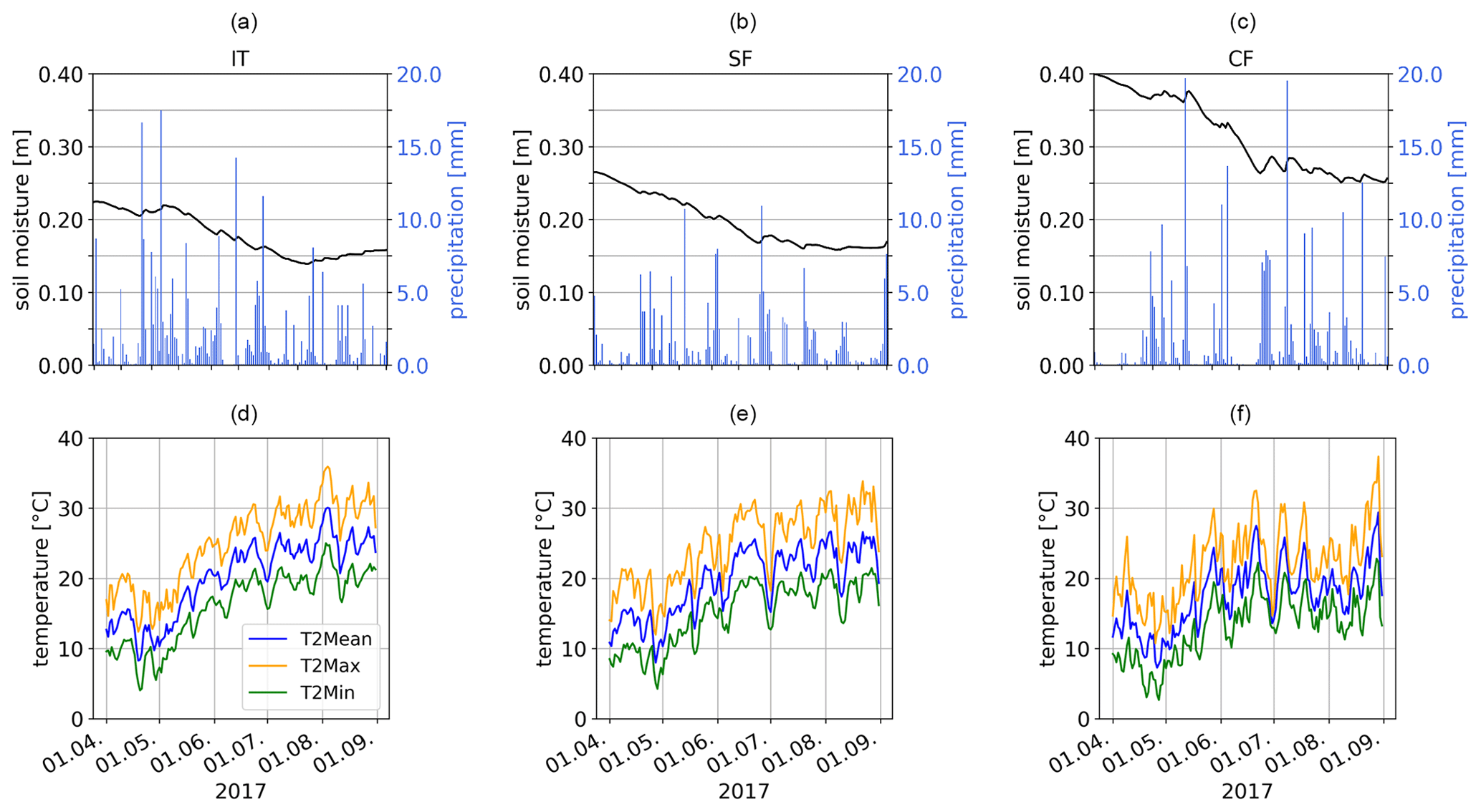
Figure 7Meteorological conditions as spatial means of the analysis regions IT, SF, and CF in 2017 for AMJJA for (a–c) soil moisture and precipitation, as well as (d–f) 2 m temperatures.
4.4 Process analysis of irrigation effects
To understand the effects of the irrigation parameterization, we analyze the results of the extreme scenario, in which the irrigation threshold and the irrigation target are wsmx of the soil; this is the maximum possible value of irrigation effects. This setting causes everyday irrigation during the growing season, resulting in soil moisture close to wsmx in the irrigated grid cells.
4.4.1 Effects on soil and surface fluxes
The irrigation effects are analyzed in terms of their spatial distribution as well as their occurrences in the diurnal and annual cycles. The soil moisture is directly increased by the parameterization, which is shown in Fig. 8a as a mean of the irrigated months April, May, and June (AMJ). Depending on the local wsmx of the soil and the actual soil moisture, the irrigation requirements in each grid cell differ from each other. Figure 8a shows a north–south gradient of the irrigation requirement with the highest values of up to 600 mm in the south like in the Ebro Basin in Spain and the Balearic Islands as well as in Italy in Sardinia, Puglia, Lazio, and the Po Valley. In the northern irrigated areas such as in France, the irrigation requirement is on average 200 mm for AMJ in the model.
Irrigation effects appear in the diurnal cycle of the soil moisture (Fig. 8b). The irrigation start time is at 7:00 LT, which increases the soil moisture, slowly at first, then faster as we get closer to the end of the irrigation end time. At 17:00 LT, the maximum irrigation effect is reached for soil moisture with an increase of 202 mm as a spatial average of irrigated areas in the model domain during AMJ.
In the annual cycle, the irrigation effects start to occur from March and increase until July (Fig. 8c). In July, the irrigation effects of the soil moisture reach +300 mm as a monthly average of all irrigated areas in the model domain. In most areas of the model domain, the growing season stops in July. Therefore, the irrigation effects decrease from August until the end of the year. Nevertheless, the soil moisture remains at a higher level than in the simulation without irrigation due to irrigation in the months before.
The effects of irrigation occur in different layers of the soil temperature as well as in the surface temperature (Fig. 8d–f). In general, irrigation reduces the surface temperature (Fig. 8d). The spatial distribution of that cooling follows the changes in the surface fluxes (Fig. 9). The strongest cooling effect in the soil occurs in the Ebro Basin and in the southern Po Valley with −4 K as a mean value in AMJ. The cooling at the surface propagates to the deeper layers of the soil, which is shown in the diurnal and annual cycle of the soil temperatures at different depths (Fig. 8e–f). The upper three layers up to a depth of 1.232 m are influenced by the surface processes. In Fig. 8e, the effects on the upper soil temperature from 0.0 to 0.065 m follow the solar radiation, reaching maximum cooling by irrigation at 13:00 LT with −3.2 K. The temperature of the second soil layer has a time-shifted reaction and reaches its maximum cooling by irrigation at 18:00 LT with −1.9 K. The levels from 0.319 m depth no longer show a diurnal cycle; however, they show a cooling between −0.05 and −1.4 K.
Since soil reacts inertly, the irrigation effects on the soil temperature throughout the year 2017 are analyzed with monthly mean values (Fig. 8f). The same order of the magnitude of the cooling effect is shown for the different temperature layers as it is in the diurnal cycle (Fig. 8e). The upper four layers react immediately to irrigation and show a cooling from March where the upper layer at the surface reaches a cooling of up to −1.5 K and the fourth layer at 1.232 m depth reaches a cooling of −0.05 K. The two upper layers reach their maximum cooling effect in April, whereas the third layer reaches its maximum cooling effect in July, the fourth layer in August, and the fifth layer in December. This time shift shows the inertial reaction of the soil temperature. The cooling of the three upper soil layers develops in spring (from March) and summer months until the harvest in July begins in wide areas of the model domain. From August the cooling effect is reduced in the upper three layers.
In general, the cooling in the soil temperature is mainly explained by two processes. First, surface processes like the enhanced latent heat flux and evaporation cool the surface temperature. This cooling slowly propagates in deeper levels. Secondly, the cooling is caused by the soil-moisture-dependent heat capacity and thermal conductivity, which increase with higher soil moisture (Eggert, 2011). This leads to faster signal transmissions and thus to faster cooling rates.
In the irrigated months AMJ, irrigation leads to an increase in evapotranspiration with the maximum in the Ebro Basin, Sardinia, and Lazio with an evapotranspiration increase of up to +150 mm (Fig. 8g). The magnitude of the increase depends on the local meteorological condition, the soil moisture, and the state of vegetation. Furthermore, in REMO2020–iMOVE, evapotranspiration is composed of evaporation from bare soil, transpiration from vegetation, and evaporation from the skin reservoir. In the diurnal cycle (Fig. 8h), the evapotranspiration increase reaches its maximum at 13:00 LT, the hour with the highest solar radiation in the model domain. During AMJ the increase in the evaporation of bare soil drives the changes in evapotranspiration. Evaporation from the skin reservoir shows negligible effects, as it is only affected by the LAI and the occurrence of precipitation or dew. Transpiration from vegetation shows a reduction through irrigation in comparison to the non-irrigated simulation from 9:00 LT to 16:00 LT in AMJ. Figure 8i shows the annual cycle of the effects on the different evaporative fractions. The transpiration from vegetation is reduced with irrigation for March, April, and May before it shows an increase from June to September of up to +14 mm per month. The reduction in spring is explained by the slower development of the LAI (Fig. 14a–b) in the irrigated simulation due to lower air temperatures (Fig. 11), which lead to reduced transpiration. In different seasons of the year, different evaporative fractions are the driver of evapotranspiration (Fig. 8i). Bare soil evaporation increases with irrigation and is the main driver of irrigation effects in evapotranspiration until July with the highest increase of +28 mm per month in April. Once the LAI reaches its maximum in July (Fig. 14a), it becomes the driver of evapotranspiration. After the crops are harvested, there is only evaporation from bare soil and from the skin reservoir.
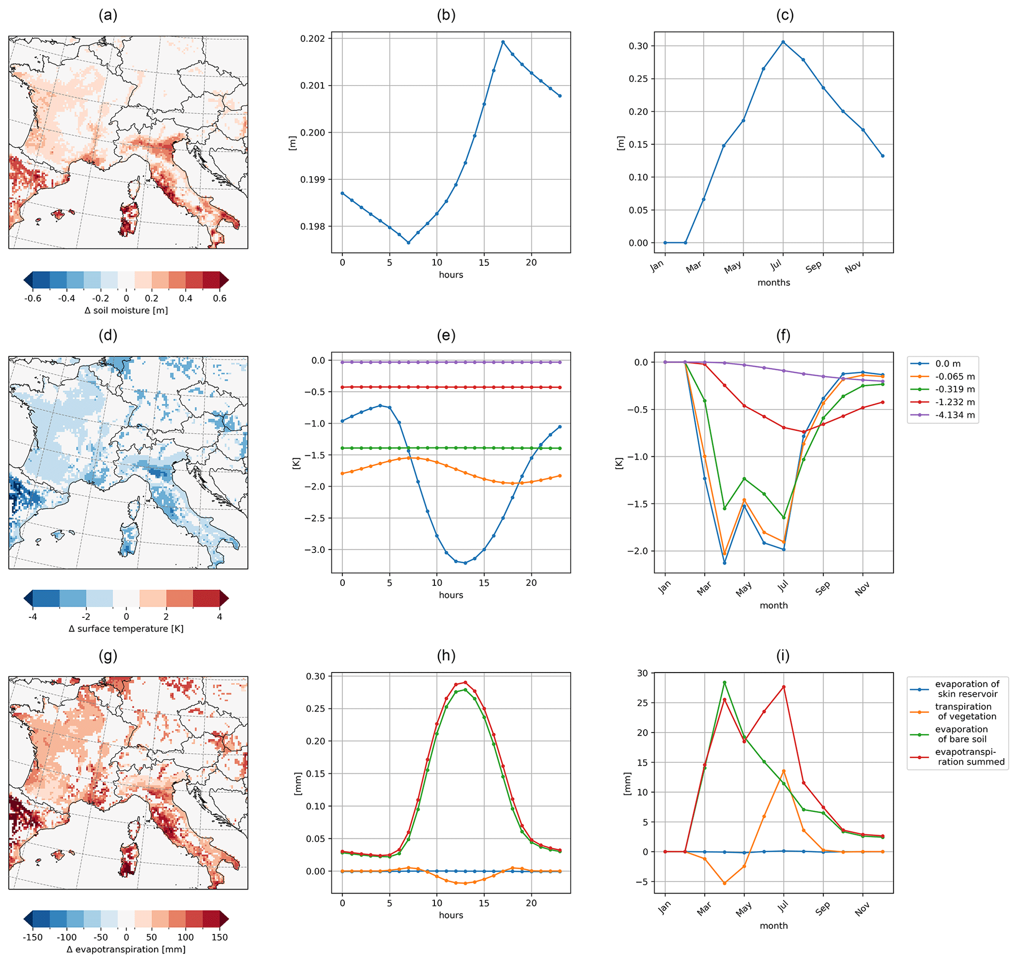
Figure 8Irrigation effects based on the difference between the simulation with irrigation (S1) and the simulation without irrigation (S0) on soil and surface processes for the irrigated fraction (a, d, g) as a spatial distribution of mean values of AMJ, (b, e, h) as a diurnal cycle of mean values of irrigated areas in AMJ, and (c, f, i) as an annual cycle of mean values of irrigated areas for (a–c) soil moisture, (d–f) soil temperature at different depths, and (g–i) evapotranspiration fractions.
Irrigation affects the surface energy budget by changing the energy fluxes (Fig. 9). The latent heat flux increases by up to +150 W m−2 and the sensible heat flux decreases by up to −120 W m−2 in the Ebro Basin, Sardinia, and Lazio during April, May, and June. These changes lead to a shift in and a reduction of the Bowen ratio by up to −1 (Fig. 9a–c), which shows that the energy transfer between the surface and the atmosphere is driven by evaporative fluxes rather than sensible heat fluxes.
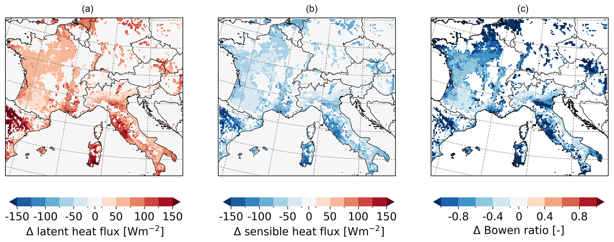
Figure 9Irrigation effects based on the difference between the simulation with irrigation (S1) and the simulation without irrigation (S0) on surface fluxes as a spatial distribution of means for AMJ for (a) latent heat flux, (b) sensible heat flux, and (c) Bowen ratio shift.
Irrigation effects on the surface energy balance in the irrigation hotspot regions show a diurnal cycle and are most pronounced during noon (Fig. 10). In SF, we see the strongest effects. There, irrigation increases the latent heat flux by up to +200 W m−2, whereas it reduces the sensible heat flux by up to −185 W m−2 during AMJ. The net radiation is slightly reduced in all three analysis regions, which can be explained by a combination of lower surface temperature (Fig. 8d), reduced surface albedo due to higher soil moisture, and increased humidity in the atmosphere with altered cloud cover. The ground heat flux is calculated as a residuum in the surface balance. During the irrigation hours, it decreases in all three analysis regions and causes less heat storage in the ground.
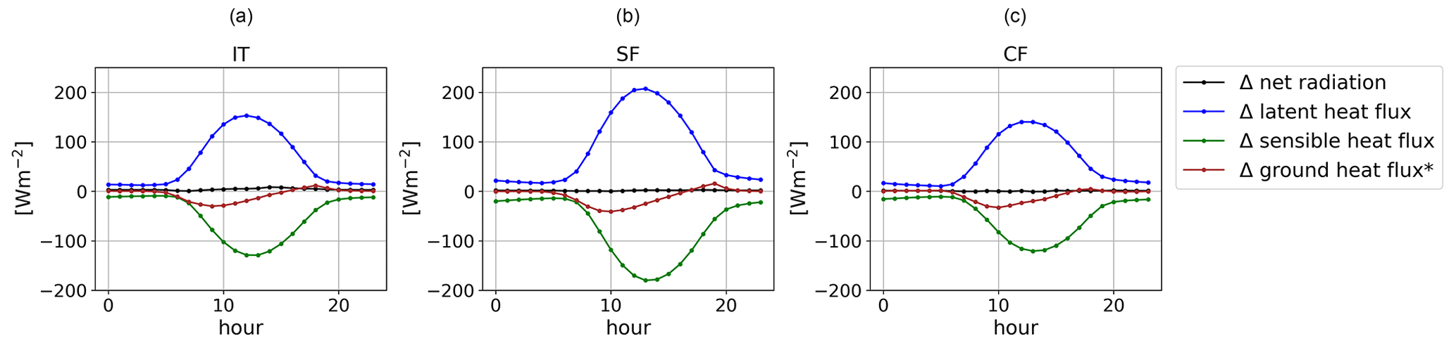
Figure 10Irrigation effects based on the difference between the simulation with irrigation (S1) and the simulation without irrigation (S0) on the surface energy balance of the irrigated fraction as hourly mean values of AMJ in the analysis regions (a) IT, (b) SF, and (c) CF.
4.4.2 Effects on the atmosphere
The effects of irrigation propagate to the atmosphere through land–atmosphere interactions, in particular through fluxes. The effects occur mostly in grid cells with a high proportion of irrigated areas like in the Po Valley and the Ebro Basin (Fig. 11a and d). In both regions, the irrigation effects on the 2 m mean temperature (T2Mean) reach a reduction of up to −2 K averaged over AMJ. Figure 11b shows the diurnal cycle of T2Mean effects in the irrigated areas of the model domain. The whiskers and the outliers show the range of irrigation effects. Overall, T2Mean is reduced starting with the irrigation at 7:00 LT and reaches the highest reduction at 14:00 LT with about −3 K in irrigated areas. After that, the temperature reduction declines until the next irrigation starts at 7:00 LT the next day. We can find outliers showing a slight temperature increase, which is connected to grid cells with a low proportion of irrigated areas. Overall, the median shows a temperature reduction of −0.3 K in the irrigated areas of the model domain.
In Fig. 11c, the monthly mean of the irrigation effect on the 2 m daily maximum (T2Max), minimum (T2Min), and T2Mean is shown. T2Max shows the strongest irrigation effects, whereas T2Min shows the smallest. The effects develop within the first irrigation month in March and reduce the 2 m temperatures. In the course of the year, the effects increase until irrigation stops in August, which is the first not completely irrigated month. As a mean of the irrigated areas in the model domain, the highest temperature reduction for T2Max and T2Mean is reached in July with −0.68 and −0.39 K, respectively. In contrast, T2Min reaches its strongest temperature reduction in April with −0.21 K. With the end of irrigation the temperature reduction declines from August for the 2 m temperatures. T2Min reaches a temperature increase in the simulations with irrigation from September to November, which can be explained by the higher humidity in the atmosphere and its higher heat absorption as the driving effect. During the growing season, this effect is masked by the evaporative cooling from vegetation and soil. In May, the temperature reduction declines due to the smaller irrigation requirement.
The increases in the latent heat flux (Fig. 9b) and the evaporation (Fig. 8g–i) lead to an increase in the 2 m relative humidity (Fig. 11d–f). As for the 2 m temperature, the irrigation effects are particularly pronounced in grid cells with a high proportion of the irrigated fraction, as in the Po Valley and the Ebro Basin. The 2 m relative humidity increases in these grid cells by up to +20 % as a mean for AMJ. Areas with smaller irrigated fractions reach a 2 m relative humidity increase of +8 %. This wide range of effects also occurs in the diurnal cycle, where the strongest irrigation effects develop in the evening hours after the irrigation stops (Fig. 11e) and the air temperature starts to decrease. Then, the relative humidity increases by up to +23 % in single grid cells. However, the median for the irrigation effect on 2 m relative humidity is at +3 %. In the annual cycle, the irrigation effect on 2 m relative humidity starts with irrigation in March. March and April, as the first irrigated months, reach the highest 2 m relative humidity increase through irrigation because these are the months with the highest irrigation requirement. In the course of the year, the irrigation effects decline to a minimum in October with less than 1 % as a spatial mean of the irrigated areas (Fig. 11f).
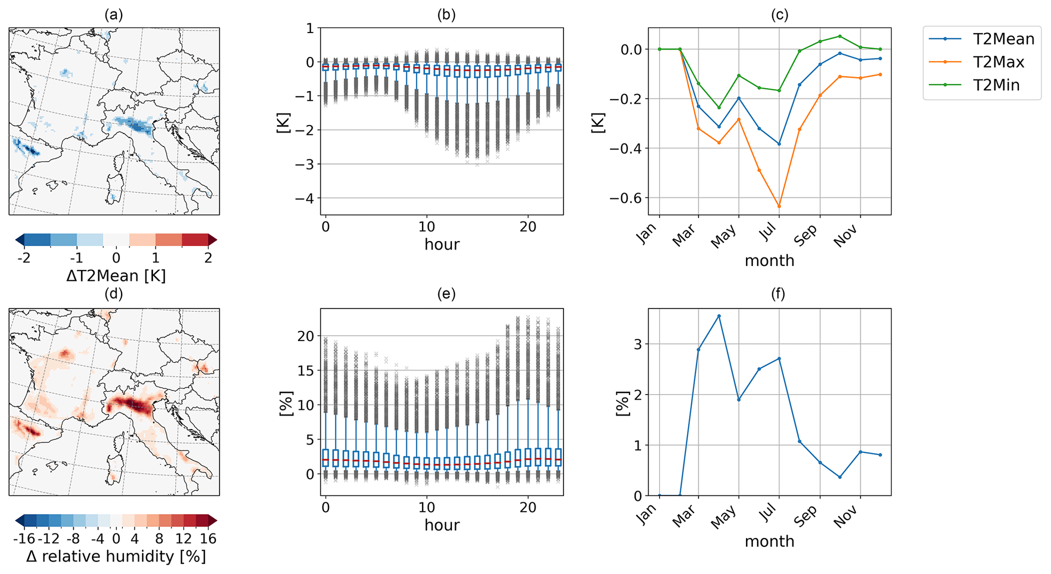
Figure 11Irrigation effects based on the difference between the simulation with irrigation (S1) and the simulation without irrigation (S0) on the atmosphere above irrigated areas as (a, d) a spatial distribution of mean values of AMJ, (b, e) a mean diurnal cycle in AMJ (with the box spanning the 1st to the 3rd quartile, the red line showing the median, the whiskers showing the 5th and 95th percentile, and outliers as values outside these limits), and (c, f) an annual cycle of mean values for (a–c) 2 m temperatures and (d–f) 2 m relative humidity.
For precipitation, the effects of irrigation are not as clear as for the 2 m temperatures and 2 m relative humidity (Fig. 12). In the spatial distribution, there is no clear pattern of the irrigation effects (Fig. 12a). There are areas along the Alps in which precipitation increased by +100 mm as a monthly mean value for AMJ. However, the pattern is very patchy. As monthly mean values for the whole model domain, the precipitation increases slightly during the irrigated months from March to July (Fig. 12b and c). After irrigation stops in July, precipitation shows a reduction in comparison to the non-irrigated simulation in August and September before it increases again from October to December. In our model setup, precipitation is represented with the shallow convection parameterization. To be able to analyze the physical processes that affect precipitation, we would have to resolve convection.
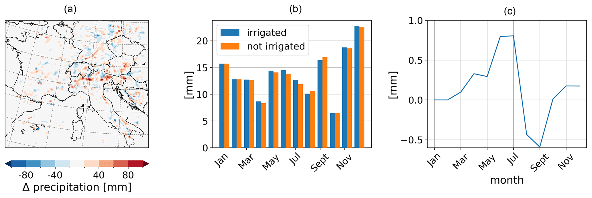
Figure 12Irrigation effects based on the difference between the simulation with irrigation (S1) and the simulation without irrigation (S0) on summed precipitation above irrigation areas as (a) a spatial distribution of mean values of AMJ, (b) monthly mean values of the irrigated and not irrigated simulation, and (c) monthly mean effects.
4.4.3 Effects on the vegetation
For the vegetation modules of iMOVE, soil moisture is a crucial variable that drives multiple plant processes, such as the growing and shedding of leaves represented in the LAI. In addition, the LAI is driven by a growing degree threshold of temperature, simulating the growing season. Reaching the growing degree threshold, the LAI will decrease through harvest in the model. Due to the warm summer, the growing season ends in the southern parts of the model domain in the middle of July. As shown in Fig. 13a–c, the irrigation effects on the LAI depend on the month, in particular on the progressing growing season, and on the region. In April and May (Fig. 13a and b), the LAI decreases in wide parts of the model domain such as central France (Fig. 13b) by −1 m2 m−2. This negative irrigation effect is caused by the 2 m temperature reduction (Fig. 11a–c), which is one of the drivers of LAI development leading to slower LAI growth in the first months of the growing season in the irrigated simulation (Fig. 14a and b). The more the growing season progresses and the vegetation approaches harvest, irrigation shows a positive effect on LAI. In June, the LAI increases with irrigation (Fig. 13c) in the Po Valley, the Ebro Basin, and Sardinia; these are areas that have experienced a warm summer and where the growing season is about to end. The LAI increases with irrigation because vegetation never experiences water stress. In June, the irrigation leads to smaller LAI in northern France as well as in parts of Germany. Again, the growing season has not yet progressed so far and the LAI develops slower with irrigation than without irrigation. The effects on the LAI mainly drive the effects on net primary production (NPP). In this study, NPP values refer to the carbon of fresh matter, following the description in Wilhelm et al. (2014). In April and May (Fig. 13d and e), the irrigation effects on NPP are very small because the growing season has not yet progressed far and vegetation just started to develop. From May onwards, irrigation increases NPP by +800 gC m−2 per month in the Ebro Basin as well as in the Po Valley. Where the LAI decreases (Fig. 13b), the NPP also decreases slightly, as in central France. In June, the NPP increases through irrigation by up to +1200 gC m−2 per month. As in the LAI, the influence of irrigation on NPP is greater as the growing season progresses. The LAI and the NPP reach their maximum in June in both simulations, with and without irrigation (Fig. 14a and c). The maximum irrigation effects of the LAI and NPP are reached shortly before the harvest in July (Fig. 14).
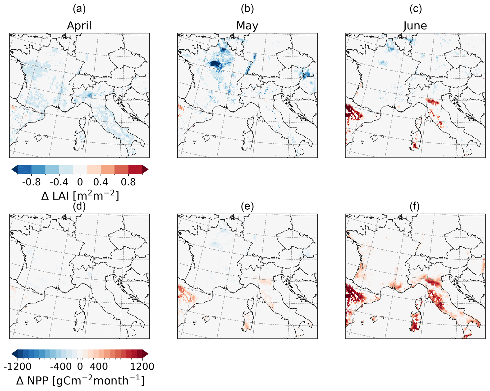
Figure 13Irrigation effects based on the difference between the simulation with irrigation (S1) and the simulation without irrigation (S0) on vegetation as a spatial distribution of monthly mean values of the irrigated fraction of (a–c) LAI and (d–f) NPP of cropland in carbon of fresh matter.

Figure 14Development of (a) LAI and (c) NPP, as well as the irrigation effects based on the difference between the simulation with irrigation (S1) and the simulation without irrigation (S0) on (b) LAI and (d) NPP of the irrigated fraction.
4.4.4 Delayed effects during a heat wave
As described in Sect. 4.3, SW Europe, particularly Italy, experienced a heat wave in early August 2017. Therefore, we will focus on the region IT including the Po Valley with its high fraction of irrigated areas for this analysis (Fig. 3). Due to its temperature-reducing effect (Fig. 11a–c), irrigation is able to reduce the intensity of heat waves. In our experiment, irrigation is performed exclusively in the growing season. The growing season depends on the 2 m temperature. In 2017, the summer in IT was exceptionally warm and the growing season ended in July (Fig. 14a); thus, there was no irrigation during the August heat wave in IT (Fig. B1). Nevertheless, irrigation shows delayed effects. Even if there was no active irrigation, the 2 m temperature is reduced during the heat wave by previous irrigation. T2Mean is reduced by up to −4.5 K and T2Max is reduced by up to −6.6 K. As with active irrigation (in AMJ, Sect. 4.4.2c), the reduction of T2Min is smaller than for the maximum temperature and reaches −2.5 K in the northwestern part of IT (Fig. 15b and c). Figure 16a shows the 2 m temperature development during the week of the heat wave from 1 August until 7 August for IT. In both simulations the hottest days are 3 and 4 August; however, T2Max is reduced by −1.5 K in the irrigated simulation, reaching 35 ∘C instead of more than 36 ∘C. After the peak of the heat wave, the 2 m temperature drops from 5 August in both simulations. In the irrigated simulation, the relative soil moisture stays close to saturation at a high level of 0.91 of wsmx after irrigation stopped, whereas in the non-irrigated simulation, it stays at a low level of 0.45 of wsmx (Fig. 16b). In IT, precipitation (Fig. 16c) occurs on 2 and 3 August at very low rates, which can be neglected, and on 5, 6, and 7 August at higher rates up to 4.5 mm d−1 in the non-irrigated simulation and 2.5 mm d−1 in the irrigated simulation. However, these precipitation rates are very low and affect the soil moisture with a small increase from 0.45 of wsmx to 0.47 of wsmx in the non-irrigated simulation on 5 August. As in Sect. 4.4.2, the effect of irrigation on precipitation is unclear during the heat wave. In Fig. 16c, in the irrigated simulation precipitation increases on 5 August, decreases on 6 August, and stays the same on 7 August. A possible explanation for the precipitation increase might be the higher evapotranspiration rate and higher relative humidity (as shown in Sect. 4.4.2). However, the temperature changes through irrigation can also affect wind patterns so that the humidity is advected outside our analysis region IT. Further, the cooling effect of irrigation on the surface temperature and near-surface temperature leads to fewer convective processes, which might have developed in the non-irrigated simulation on 6 August. During the heat wave, transpiration of the remaining vegetation and evaporation of the soil are the drivers of evapotranspiration (Fig. 16d). However, in the irrigated simulation the evapotranspiration rate with up to 4 mm d−1 is almost double the evapotranspiration rate if irrigation is not turned on. This difference can be explained by the evaporation of bare soil. In the irrigated simulation the soil remained close to saturation (Fig. 16b) and can evaporate. In the non-irrigated simulation, the soil moisture is at a very low level and barely evaporates (Fig. 16d). After the precipitation events, the skin reservoir also evaporates on 6 and 7 August.
The delayed irrigation effects decrease the intensity of the heat wave and provide moisture in the soil to be evaporated, which can prevent the wilting of vegetation.
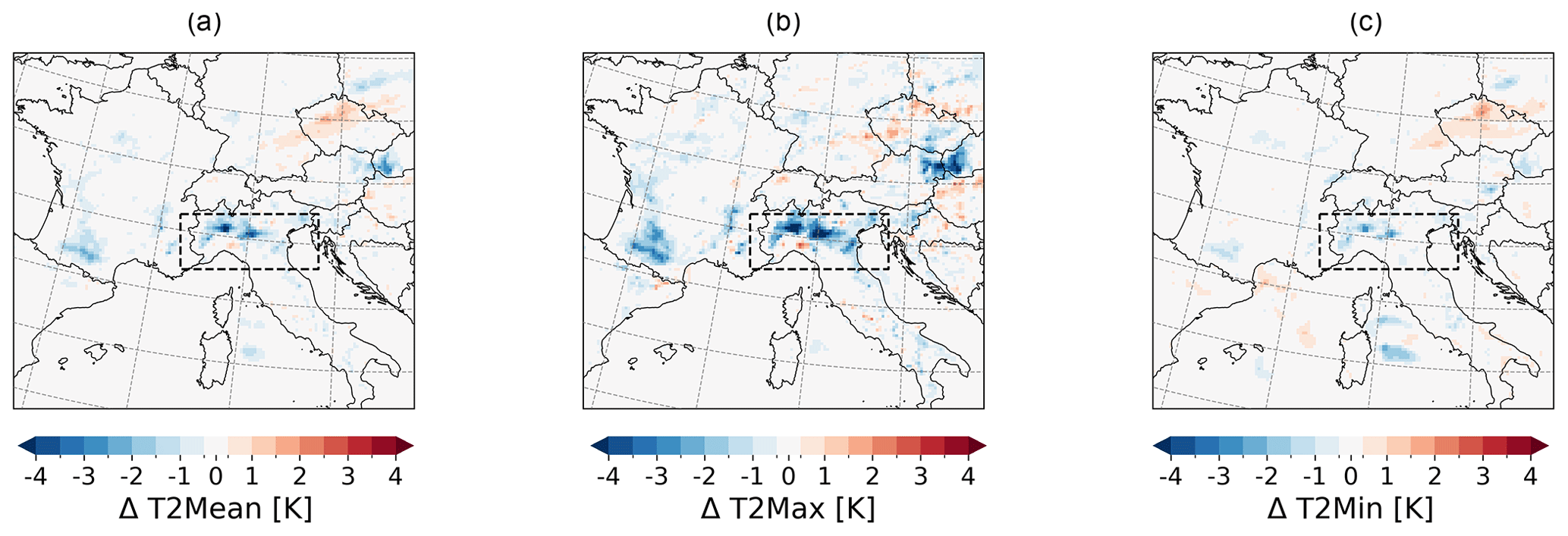
Figure 15Delayed irrigation effects based on the difference between the simulation with irrigation (S1) and the simulation without irrigation (S0) on 2 m temperature during the heat wave from 1–7 August 2017 in IT: (a) T2Mean, (b) T2Max, and (c) T2Min.
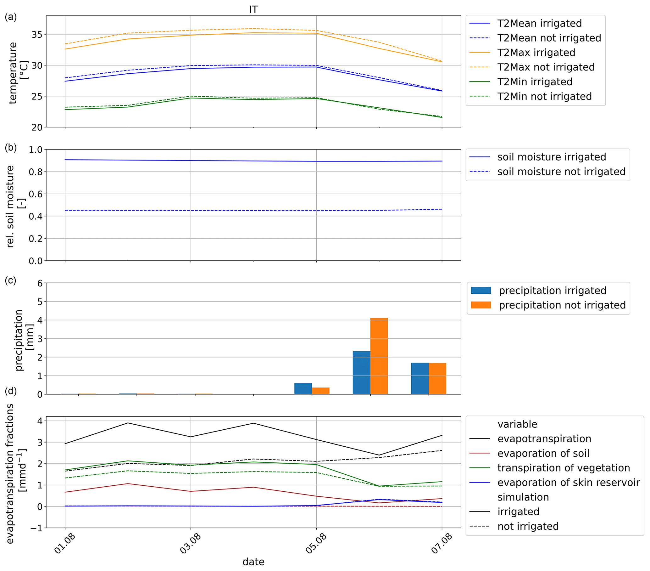
Figure 16Development of delayed irrigation effects based on the difference between the simulation with irrigation (S1) and the simulation without irrigation (S0) during the heat wave in August (1–7 August 2017) in IT as (a) a spatial mean of 2 m temperatures, (b) a spatial mean of relative soil moisture, (c) a spatial sum of precipitation, and (f) a spatial mean of evapotranspiration.
4.5 Comparison with observational data
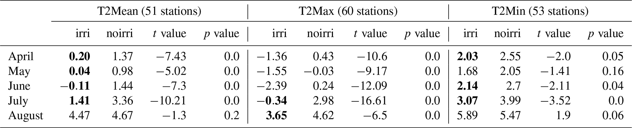
The results of the simulations are compared to observational data collected within SCIA (Sect. 2.3). For the comparison, we have focused exclusively on the Po Valley, represented in the analysis region IT (Fig. 3). In the Po Valley, we have the largest cluster of grid cells with a high proportion of irrigated fraction (Fig. 3) and therefore the most developed irrigation effects in the atmosphere. To compare the model results to the observational data, we filtered the SCIA data for April to August, as months with active irrigation, as well as months with delayed irrigation effects. Further, we filtered the SCIA data for the location in the IT region and the presence of an irrigated fraction. We selected the SCIA data with an irrigated fraction higher than 31 %, which is the mean of the irrigated fraction in that area, to reach a clear signal from the irrigation effects. The model data were then interpolated to the locations of the filtered observational data using inverse distance weighting with four known points. We calculated the bias for each station location and averaged it across all locations for each month. As the last step, the statistical significance of the bias distributions is evaluated with a Student's t test for two independent samples using a significance level (α) of 0.05. This process was performed for the results from the simulation with irrigation as well as for the results from the simulation without irrigation. The filtering results in a different number of suitable station data for each variable (Table 3, Fig. C1).
For this comparison, we focus on the near-surface temperature variables T2Mean, T2Max, and T2Min. In general, the irrigation parameterization reduces the 2 m temperatures. Without irrigation, REMO2020–iMOVE overestimates T2Mean from April to August in IT. Using the irrigation parameterization, the bias can be significantly reduced from April to July, in particular in May with a remaining bias of 0.04 K. However, July and especially August have the largest bias in the irrigated and non-irrigated simulation results. The delayed irrigation effects cause only a minor, nonsignificant bias reduction in August from 4.67 K in the non-irrigated simulation to 4.47 K in the irrigation simulation. The large biases in July (irrigated: 1.41 K, not irrigated: 3.36 K) and August are most probably connected to the early harvest and the drop in vegetation. Vegetation is an important contributor to the evapotranspiration of the surface, which has a cooling effect on the 2 m temperature (Fig. 8g–i). The early harvest and the early end of the growing season lead to an end of active irrigation.
For T2Mean, the irrigation parameterization caused significant bias reductions from April to July with high t values and p values of 0.0. For T2Max and T2Min, the results are not as clear as for T2Mean. REMO2020–iMOVE overestimates T2Max in April, June, July, and August. Using the irrigation parameterization leads to an underestimation of T2Max, except for August when the delayed cooling effect of irrigation reduces the large bias of 4.61 to 3.65 K. Again, August has the largest bias in both simulations and can be explained by the drop in vegetation. In general, T2Max is represented closer to observational values without irrigation.
The T2Min is overestimated with and without the irrigation parameterization by REMO2020–iMOVE. However, the irrigation parameterization significantly reduces the bias in April, June, and July. As for T2Mean and T2Max, August is the month with the largest bias in both simulations. However, the irrigation parameterization increases the bias even more from 5.47 to 5.89 K this time with its warming effect in August for T2Min (Fig. 11). The results for T2Min show lower t values and larger p values, pointing out the lower robustness of the bias distributions.
Table 3The 2 m temperature bias for the irrigated and non-irrigated simulation with t-test results. Bold values indicate statistical significance with α=0.05.
We developed a new subgrid parameterization representing channel irrigation and implemented it in the regional climate model system REMO2020–iMOVE. An older version of the model, REMO2009, was previously tested with an irrigation parameterization by Saeed et al. (2009). The study analyzed large-scale irrigation effects over the Indian subcontinent at 0.5∘ horizontal resolution. In contrast to our study, the parameterization represented irrigation in the whole model grid cell, leading to possible overestimation of irrigation effects. However, it pointed out the importance of representing irrigation in climate models, in particular over large-scale, intensely irrigated areas such as the Indus Basin because irrigation decreases dry biases and affects the development of meteorological patterns such as the South Asian summer monsoon by adding water to the climate system (Saeed et al., 2009). In our experiment, we focus on higher-resolution simulations. The representation of irrigation on a subgrid scale is an improvement in the representation of irrigated areas and qualifies the parameterization for high-resolution studies in heterogeneous regions such as Europe. According to Im et al. (2010) and Giorgi and Avissar (1997), subgrid-scale representation of land cover and land use improves the representation of land–atmosphere interaction in climate models. In the new parameterization, irrigation is exclusively realized where it is required. Therefore, only the irrigated fraction is part of the irrigation process. The subgrid-scale approach is also used in, e.g., Lawrence et al. (2019) and Ozdogan et al. (2010). Our irrigation parameterization has different water application schemes that can be used to address different research questions. An influence of the different water application schemes on irrigation effects could not be found for similar settings. However, it has to be considered that the irrigation effects depend strongly on the irrigation amount, which in turn depends on the soil hydrology of the climate model. Due to the bucket scheme in REMO2020–iMOVE, suitable prescribed values of the irrigation amount differ from observed values because the water is added to the whole soil column. Therefore, model-specific values need to be chosen and the irrigation amount cannot be validated with observational values. However, to simulate irrigation effects, irrigation using physical thresholds as the irrigation start and target, as in the flextime and adaptive water application scheme, is more suitable and able to represent realistic soil conditions. For the future, for irrigation studies, we recommend the representation of the soil hydrology with a multiple-layer scheme as in WRF (Valmassoi et al., 2020c) and CLM (Lawrence et al., 2019; Ozdogan et al., 2010); it already exists and was developed for REMO2015 (Abel, 2023). A multiple-layer scheme will allow the usage of observed values for the irrigation amount and improves the representation of soil hydrology. Further, to represent an observed irrigation amount, irrigation water loss through, e.g., evaporation or leaks during water transport, has to be considered. Our irrigation parameterization adds the irrigation water directly to the soil moisture and therefore does not take into account irrigation efficiency.
For REMO2020–iMOVE and its bucket scheme, we selected the adaptive water application scheme as the default scheme because it does not require model-specific values and reaches the irrigation target in the prescribed time. To the authors' knowledge, a nonlinear approach, such as the adaptive scheme, has never been used for irrigation parameterization before but has proven to be suitable in this study.
The simulated effects of the irrigation parameterization on the surface energy balance are more pronounced in our study than in comparable studies (Valmassoi et al., 2020b; Lobell et al., 2009). This can be explained by the newly implemented fraction that has its own surface energy balance. In this study, we exclusively analyzed the values of the irrigated fraction and no grid cell averages of the soil and surface variables. Further, in our experiment, we used the maximum irrigation target and the maximum irrigation threshold to show the maximum possible effects. The effects on the atmosphere are in the same range as other studies (Valmassoi et al., 2020b; Lobell et al., 2009; Thiery et al., 2017). For example, Valmassoi et al. (2020b) found a monthly T2Max reduction of up to −3 K in the Po Valley, whereas we found a T2Max reduction of up to −4 K in single grid cells. The effect on vegetation, slowing down the development of the LAI, is model-specific and could not be verified with other studies. In contrast, studies found that with irrigation the LAI is larger than without (Patanè, 2011). Therefore, the interactive LAI representation in REMO2020–iMOVE might have to be improved. Further, the large positive bias in August in comparison to observational data can be attributed to the missing vegetation and the early harvest in July, which is represented as an LAI drop, causing a stop to vegetation processes. The missing evaporative cooling of the transpiration of vegetation leads to increasing 2 m temperatures. This effect was already observed by Wilhelm et al. (2014) and Rai et al. (2022). Nevertheless, the irrigation parameterization could significantly reduce the bias for T2Mean in 2017 in the Po Valley, particularly in months with active irrigation. For T2Max, the irrigation parameterization adds a cold bias, whereas, for T2Min, the irrigation parameterization reduces the warm bias. We can infer that the irrigation parameterization decreases the diurnal range of the 2 m temperature. However, as the warm bias in T2Min is also still high with irrigation, other processes in the model need to be considered as the source. The underestimation of T2Max can be traced back to our experiment design, which shows maximum irrigation effects. Therefore, it might overestimate irrigation effects. First, our irrigated fraction is based on the area equipped for irrigation that is not completely irrigated in reality. Second, in our experiments, we keep the soil moisture at very high levels (higher than 0.75 of wsmx) at which plants do not experience any water stress and the potential transpiration by plants is reached. And third, we irrigate in daytime hours, leading to strong effects on variables with a distinct diurnal cycle such as the surface fluxes, evapotranspiration, and T2Max. The effect of irrigation timing was analyzed by Valmassoi et al. (2020c), who showed a rather low impact of irrigation timing on the development of irrigation effects.
For our irrigation parameterization, we assumed unlimited water availability for all grid cells. However, for irrigation practice, this is not the case. First, the probability of heat waves and droughts in western and southern Europe increases with climate change (Kew et al., 2019) and there is likely not sufficient water available during these periods (IPCC, 2019). Second, during heat waves and droughts, governments have to ration water, as happened during the intense heat wave in 2022 in northern Italy (Balmer and Amante, 2022; Giuffrida, 2022). Having a limited water reservoir in REMO2020–iMOVE would be a step towards a more realistic irrigation amount.
Our parameterization increases the soil moisture directly and can therefore be understood as a representation of channel irrigation. Additionally, there are more irrigation methods, e.g., sprinkler or drip methods, which require canopy interactions and different parameterization approaches as Valmassoi et al. (2020c) and Yao et al. (2022) pointed out.
In our study irrigation effects on precipitation remain unclear and cannot reproduce the findings in observation studies showing a regional annual decrease in precipitation as found in Szilagyi and Franz (2020). However, irrigation effects on precipitation are indirect and influenced by many interconnected factors such as atmospheric stability, specific humidity, temperature, and wind patterns. These make a comparison difficult. To find clearer patterns of irrigation effects on precipitation, a longer experiment is necessary. Further, in our study, the convective precipitation is parameterized and the generating processes are not resolved. Therefore, we recommend using convection-permitting resolution for analyzing precipitation–irrigation feedback.
By implementing irrigation into the regional climate model system REMO2020–iMOVE, we include a widely used land use practice and an important aspect of anthropogenic forcing on the climate system, enabling the investigation of irrigation effects. Our newly developed parameterization is designed for high-resolution studies using a separate irrigated land fraction, ensuring that exclusively irrigated areas are irrigated in the model and irrigation effects can be realistically estimated. Further, our parameterization takes into account vegetation processes. With our model system REMO2020–iMOVE, we could show the irrigation effects and feedbacks regarding LAI development, which develops slower in the model but reaches higher maxima, and regarding the process of NPP, which increases with irrigation. Our parameterization is characterized by three water application schemes, which simulate irrigation with prescribed irrigation, with flexible time irrigation, and with adaptive irrigation. Even though the irrigation schemes differ in irrigation time, irrigation events, and water application per time step, the differences in the effects are small and can be neglected. However, the different irrigation schemes can be applied to different research questions in the future. Rather than the water application, the water amount is an important driver of irrigation effects. Therefore, simulations with a realistic irrigation amount together with a layer model are desirable for the future.
We applied our irrigation parameterization for dry and hot conditions in 2017 in SW Europe. Whereas the effects on soil and surface variables are more pronounced in our study using the fractional approach than in comparable studies, the effects on the atmosphere match the range of temperature reduction. For effects on small-scale precipitation, the resolution of our study is not high enough and we cannot resolve convective processes, leading to unclear irrigation effects. Therefore, studies with higher resolution, such as on a convection-permitting scale, and with a longer extent are necessary. For REMO2020–iMOVE the application of our irrigation parameterization significantly decreased the monthly warm bias of T2Mean during AMJ with active irrigation. But delayed irrigation effects also occur, influencing the summer season. Our study showed that irrigation effects such as temperature reduction and soil moisture increase are not only an adaptation measure during droughts or heat waves, but also that these irrigation effects have the potential to prevent or mitigate such climate extremes on a local scale.
A1 Implementing irrigation into REMO2020–iMOVE
A2 Water application schemes
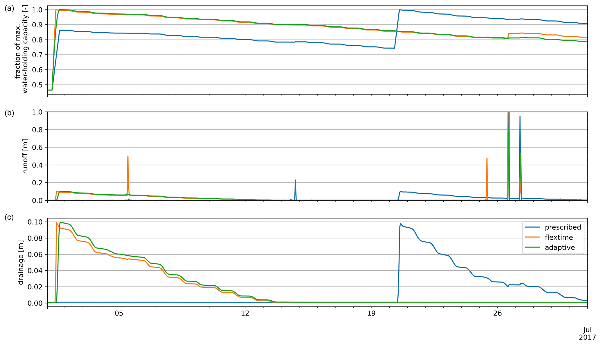
Figure A2Results of different water application schemes (T1, T2, T3) for (a) relative soil moisture, (b) runoff, and (c) drainage.
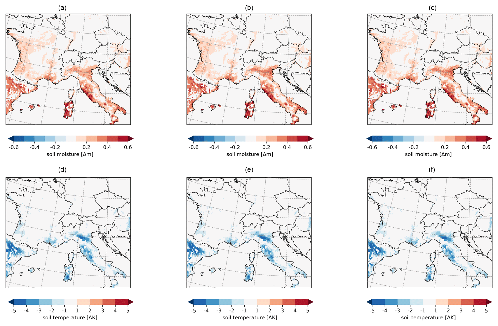
Figure A3Spatial distribution of the mean effects of different water application schemes in June 2017 for (a)–(c) soil moisture and (d)–(f) surface temperature using the (a, d) prescribed, (b, e) flextime, and (c, f) adaptive scheme.
Figure A4Differences between water application schemes in June 2017 for (a–b) soil moisture and (c–d) surface temperature between (a–c) the flextime and prescribed schemes and between (b–d) the adaptive and prescribed schemes.
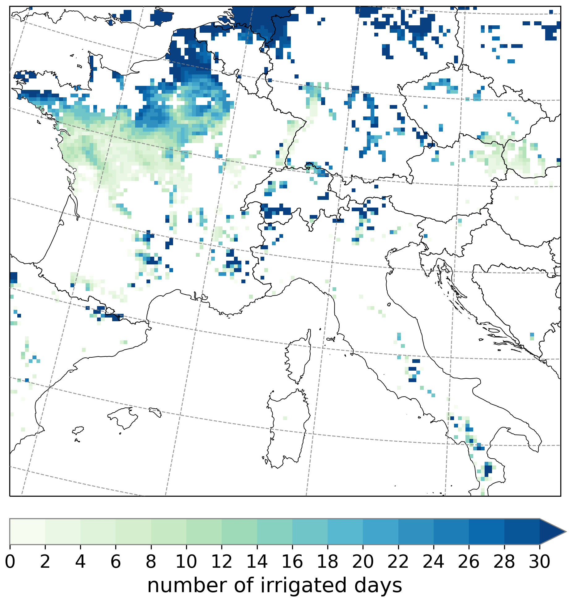
Figure B1Number of irrigation days in August 2017.
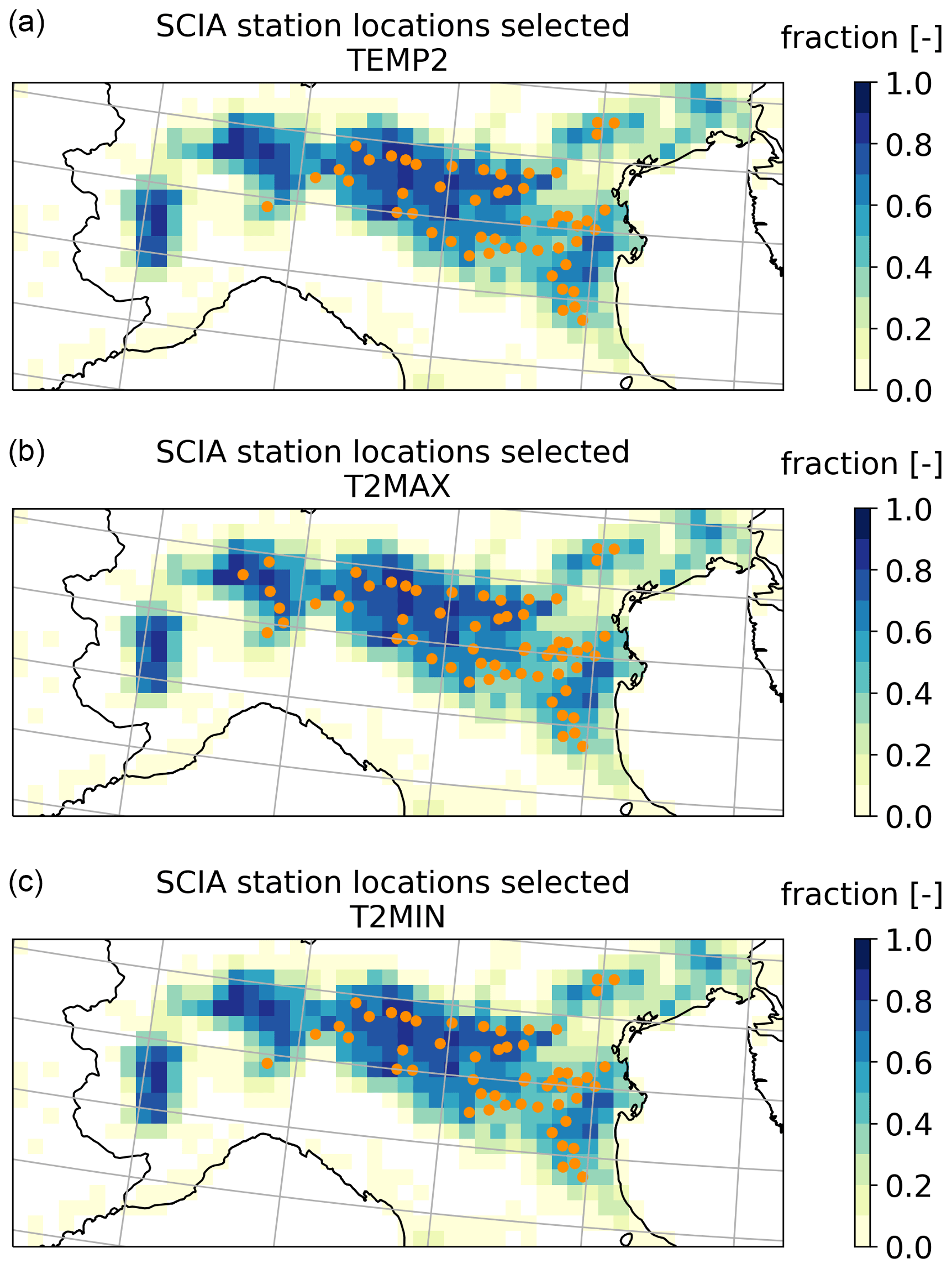
Figure C1Station location for (a) T2Mean, (b) T2Max, and (c) T2Min.
The model code of REMO2020–iMOVE with the new irrigation parameterization is available on request (contact@remo-rcm.de).
The scripts used to produce the results presented in this paper are archived on Zenodo (https://doi.org/10.5281/zenodo.7889384, Asmus and Buntemeyer, 2023), as are the simulation data together with the observational data from SCIA (https://doi.org/10.5281/zenodo.7867328, Asmus, 2023) after we received their permission. Originally, we downloaded the observation data from http://www.scia.isprambiente.it/ (last access: 8 December 2023) using the API http://193.206.192.214/servertsutm/serietemporali400.php (Desiato et al., 2011).
CA, PH, DR, and JB developed the experiments. CA developed the irrigation module. CA and JPP implemented the parameterization in the model code in close cooperation with PH. CA conducted the analysis including the visualizations under the supervision of DR and JB. CA prepared the initial paper. All authors reviewed the paper draft and contributed to the final paper.
The contact author has declared that none of the authors has any competing interests.
Publisher's note: Copernicus Publications remains neutral with regard to jurisdictional claims made in the text, published maps, institutional affiliations, or any other geographical representation in this paper. While Copernicus Publications makes every effort to include appropriate place names, the final responsibility lies with the authors.
We are grateful for the support and help of the REMO developer team located at GERICS. We want to thank Lars Buntemeyer in particular for preparing the ERA5 data as model forcing and helping with the publication of the analysis code and data. We also thank Juliane El Zohbi for internally reviewing our paper draft. We are grateful to DKRZ for providing the high computing capacity, with which we performed our simulations. Further, we want to thank ISPRA for collecting and providing observation data publicly in the SCIA database and FAO for providing the GMIA V5 publicly.
This work was financed within the framework of the Helmholtz Institute for Climate Service Science (HICSS), a cooperation between the Climate Service Center Germany (GERICS) and Universität Hamburg, Germany, and it was conducted as part of the LANDMATE (Modelling human LAND surface modifications and its feedbacks on local and regional cliMATE) project.
The article processing charges for this open-access publication were covered by the Helmholtz-Zentrum Hereon.
This paper was edited by Hisashi Sato and reviewed by Hisashi Sato and one anonymous referee.
Abel, D. K.-J.: Weiterentwicklung der Bodenhydrologie des regionalen Klimamodells REMO, PhD thesis, Universität Würzburg, https://doi.org/10.25972/OPUS-31146, 2023. a
Asmus, C.: Modeling and evaluating the effects of irrigation on land-atmosphere interaction in southwestern Europe with the regional climate model REMO2020-iMOVE using a newly developed parameterization, Zenodo [data set], https://doi.org/10.5281/zenodo.7867328, 2023. a
Asmus, C. and Buntemeyer, L.: Modeling and evaluating the effects of irrigation on land-atmosphere interaction in southwestern Europe with the regional climate model REMO2020-iMOVE using a newly developed parameterization, Zenodo [code], https://doi.org/10.5281/zenodo.7889384, 2023. a
Balmer, C. and Amante, A.: Analysis: Wasted water saps battle against Italy's worst drought in decades, Reuters, https://www.reuters.com/world/europe/wasted-water-saps-battle-against-italys-worst-drought-decades-2022-07-19/ (last access: 30 November 2023), 2022. a
Bjorneberg, D.: IRRIGATION | Methods, in: Reference Module in Earth Systems and Environmental Sciences, Elsevier, ISBN 978-0-12-409548-9, https://doi.org/10.1016/B978-0-12-409548-9.05195-2, 2013. a
Boucher, O., Myhre, G., and Myhre, A.: Direct human influence of irrigation on atmospheric water vapour and climate, Clim. Dynam., 22, 597–603, https://doi.org/10.1007/s00382-004-0402-4, 2004. a
Copernicus Climate Change Service: European State of the Climate 2017, Climate in 2017 – Focus Region: Southwest Europe, Southwest Europe – dry conditions, https://climate.copernicus.eu/climate-2017-focus-region-southwest-europe, last access: 1 December 2023. a, b, c
Desiato, F., Fioravanti, G., Fraschetti, P., Perconti, W., and Toreti, A.: Climate indicators for Italy: calculation and dissemination, Adv. Sci. Res., 6, 147–150, https://doi.org/10.5194/asr-6-147-2011, 2011 (data available at: http://193.206.192.214/servertsutm/serietemporali400.php, last access: 8 December 2023). a, b
de Vrese, P. and Hagemann, S.: Uncertainties in modelling the climate impact of irrigation, Clim. Dynam., 51, 2023–2038, https://doi.org/10.1007/s00382-017-3996-z, 2018. a, b, c, d
Doell, P. and Siebert, S.: A Digital Global Map of Irrgated Areas, Report A9901, Center for Environmental Systems Research, University of Kassel, Kurt Wolters Strasse 3, 34109 Kassel, Germany, https://doi.org/10.13140/2.1.2726.2080, 1999. a
Dümenil, L. and Todini, E.: Chapter 9 – A rainfall–runoff scheme for use in the Hamburg climate model, in: Advances in Theoretical Hydrology, edited by: O'Kane, J. P., European Geophysical Society Series on Hydrological Sciences, Elsevier, Amsterdam, 129–157, https://doi.org/10.1016/B978-0-444-89831-9.50016-8, 1992. a
Eggert, B.: Auswirkungen der Oberflächeneigenschaften in REMO auf die Simulation der unteren Atmosphäre, CSC Report, 8, https://epub.sub.uni-hamburg.de/epub/volltexte/2013/23967/pdf/csc_report8.pdf (last access: 30 November 2023), 2011. a
Giorgi, F. and Avissar, R.: Representation of heterogeneity effects in Earth system modeling: Experience from land surface modeling, Rev. Geophys., 35, 413–437, https://doi.org/10.1029/97RG01754, 1997. a
Giuffrida, A.: More than 100 towns in Italy’s Po valley asked to ration water, The Guardian, https://www.theguardian.com/world/2022/jun/15/italy-drought-po-valley-ration-water (last access: 30 November 2023), 2022. a
Goettel, H.: Einfluss der nichthydrostatischen Modellierung und der Niederschlagsverdriftung auf die Ergebnisse regionaler Klimamodellierung, PhD thesis, MPI für Meteorologie, Hamburg, https://doi.org/10.17617/2.994076, 2009. a
Hagemann, S.: An Improved Land Surface Parameter Dataset for Global and Regional Climate Models, MPI Report 336, Max-Planck-Institut fuer Meteorologie, 21 pp., https://doi.org/10.17617/2.2344576, 2002. a
Hagemann, S., Botzet, M., Dümenil, L., and Machenhauer, B.: Derivation of global GCM boundary conditions 10 from 1 km land use satellite date, MPI Report No. 289, Max-Planck-Institut fuer Meteorologie, 34 pp., https://pure.mpg.de/rest/items/item_1562156_5/component/file_1562155/content (last access: 30 November 2023), 1999. a, b
Hoffmann, P., Reinhart, V., Rechid, D., de Noblet-Ducoudré, N., Davin, E. L., Asmus, C., Bechtel, B., Böhner, J., Katragkou, E., and Luyssaert, S.: High-resolution land use and land cover dataset for regional climate modelling: historical and future changes in Europe, Earth Syst. Sci. Data, 15, 3819–3852, https://doi.org/10.5194/essd-15-3819-2023, 2023. a
Im, E.-S., Coppola, E., Giorgi, F., and Bi, X.: Validation of a High-Resolution Regional Climate Model for the Alpine Region and Effects of a Subgrid-Scale Topography and Land Use Representation, J. Climate, 23, 1854–1873, https://doi.org/10.1175/2009JCLI3262.1, 2010. a
IPCC: Summary for Policymakers, in: Climate Change and Land: an IPCC special report on climate change, desertification, land degradation, sustainable land management, food security, and greenhouse gas fluxes in terrestrial ecosystems, edited by: Shukla, P. R., Skea, J., Calvo Buendia, E., Masson-Delmotte, V., Pörtner, H.-O., Roberts, D. C., Zhai, P., Slade, R., Connors, S., van Diemen, R., Ferrat, M., Haughey, E., Luz, S., Neogi, S., Pathak, M., Petzold, J., Portugal Pereira, J., Vyas, P., Huntley, E., Kissick, K., Belkacemi, M., and Malley, J., https://doi.org/10.1017/9781009157988.001, 2019. a
Jacob, D.: A note to the simulation of the annual and inter-annual variability of the water budget over the Baltic Sea drainage basin, Meteorol. Atmos. Phys., 77, 61–73, https://doi.org/10.1007/s007030170017, 2001. a
Jacob, D.and Podzun, R.: Sensitivity studies with the regional climate model REMO, Meteorol. Atmos. Phys., 63, 119–129, https://doi.org/10.1007/BF01025368, 1997. a
Jia, G., Shevliakova, E., Artaxo, P., De Noblet-Ducoudré, N., Houghton, R., House, J., Kitajima, K., Lennard, C., Popp, A., Sirin, A., Sukumar, R., and Verchot, L.: Land–climate interactions, in: Climate Change and Land: an IPCC special report on climate change, desertification, land degradation, sustainable land management, food security, and greenhouse gas fluxes in terrestrial ecosystems, edited by: Shukla, P. R., Skea, J., Calvo Buendia, E., Masson-Delmotte, V., Pörtner, H.-O., Roberts, D., Zhai, P., Slade, R., Connors, S., van Diemen, R., Ferrat, M., Haughey, E., Luz, A., Neogi, S., Pathak, M., Petzold, J., Portugal Pereira, J., Vyas, P., Huntley, E., Kissick, K., Belkacemi, M., and Malley, J., book section Chapter 2, Intergovernmental Panel on Climate Change, https://www.ipcc.ch/site/assets/uploads/sites/4/2022/11/SRCCL_Chapter_2.pdf (last access: 30 November 2023), in press, 2019. a, b
Kew, S. F., Philip, S. Y., van Oldenborgh, G. J., van der Schrier, G., Otto, F. E. L., and Vautard, R.: The Exceptional Summer Heat Wave in Southern Europe 2017, B. Am. Meteorol. Soc., 100, S49–S53, https://doi.org/10.1175/BAMS-D-18-0109.1, 2019. a, b
Kotlarski, S.: A subgrid glacier parameterisation for use in regional climate modelling, PhD Thesis, University of Hamburg, Hamburg, https://doi.org/10.17617/2.994357, 2007. a, b, c, d, e
Kueppers, L., Snyder, M., and Sloan, L.: Irrigation cooling effect: Regional climate forcing by land-use change, Geophys. Res. Lett., 34, L03703, https://doi.org/10.1029/2006GL028679, 2007. a, b, c, d, e, f
Lawrence, D. M., Fisher, R. A., Koven, C. D., Oleson, K. W., Swenson, S. C., Bonan, G., Collier, N., Ghimire, B., van Kampenhout, L., Kennedy, D., Kluzek, E., Lawrence, P. J., Li, F., Li, H., Lombardozzi, D., Riley, W. J., Sacks, W. J., Shi, M., Vertenstein, M., Wieder, W. R., Xu, C., Ali, A. A., Badger, A. M., Bisht, G., van den Broeke, M., Brunke, M. A., Burns, S. P., Buzan, J., Clark, M., Craig, A., Dahlin, K., Drewniak, B., Fisher, J. B., Flanner, M., Fox, A. M., Gentine, P., Hoffman, F., Keppel-Aleks, G., Knox, R., Kumar, S., Lenaerts, J., Leung, L. R., Lipscomb, W. H., Lu, Y., Pandey, A., Pelletier, J. D., Perket, J., Randerson, J. T., Ricciuto, D. M., Sanderson, B. M., Slater, A., Subin, Z. M., Tang, J., Thomas, R. Q., Val Martin, M., and Zeng, X.: The Community Land Model Version 5: Description of New Features, Benchmarking, and Impact of Forcing Uncertainty, J. Adv. Model. Earth Sy., 11, 4245–4287, https://doi.org/10.1029/2018MS001583, 2019. a, b
Leng, G., Huang, M., Tang, Q., and Leung, L. R.: A modeling study of irrigation effects on global surface water and groundwater resources under a changing climate, J. Adv. Model. Earth Sy., 7, 1285–1304, https://doi.org/10.1002/2015MS000437, 2015. a
Leng, G., Leung, L. R., and Huang, M.: Significant impacts of irrigation water sources and methods on modeling irrigation effects in the ACME Land Model, J. Adv. Model. Earth Sy., 9, 1665–1683, https://doi.org/10.1002/2016MS000885, 2017. a
Lobell, D., Govindasamy, B., Mirin, A., Phillips, T., Maxwell, R., and Rotman, D.: Regional Differences in the Influence of Irrigation on Climate, J. Climate, 22, 2248–2255, https://doi.org/10.1175/2008JCLI2703.1, 2009. a, b, c, d, e, f, g
Luyssaert, S., Jammet, M., Stoy, P., Estel, S., Pongratz, J., Ceschia, E., Churkina, G., Don, A., Erb, K.-H., Ferlicoq, M., Gielen, B., Grünwald, T., Houghton, R., Klumpp, K., Knohl, A., Kolb, T., Kuemmerle, T., Laurila, T., Lohila, A., and Dolman, H. A.: Land management and land-cover change have impacts of similar magnitude on surface temperature, Nat. Clim. Change, 4, 389–393, https://doi.org/10.1038/nclimate2196, 2014. a, b
Majewski, D.: The EUROPA-modell of the Deutscher Wetterdienst, in: Seminar on Numerical Methods in Atmospheric Models, 9–13 September 1991, vol. II, ECMWF, ECMWF, Shinfield Park, Reading, 147–193, https://www.ecmwf.int/node/10940 (last access: 1 December 2023), 1991. a
Ozdogan, M., Rodell, M., Beaudoing, H. K., and Toll, D. L.: Simulating the Effects of Irrigation over the United States in a Land Surface Model Based on Satellite-Derived Agricultural Data, J. Hydrometeorol., 11, 171–184, https://doi.org/10.1175/2009JHM1116.1, 2010. a, b, c, d, e
Patanè, C.: Leaf Area Index, Leaf Transpiration and Stomatal Conductance as Affected by Soil Water Deficit and VPD in Processing Tomato in Semi Arid Mediterranean Climate, J. Agron. Crop Sci., 197, 165–176, https://doi.org/10.1111/j.1439-037X.2010.00454.x, 2011. a
Peterson, J. B., Robinson, B. F., and Beck, R. H.: Predictability of Change in Soil Reflectance on Wetting, LARS Symposia, Paper 279, http://docs.lib.purdue.edu/lars_symp/279 (last access: 1 December 2023), 1979. a
Pietikäinen, J.-P., Markkanen, T., Sieck, K., Jacob, D., Korhonen, J., Räisänen, P., Gao, Y., Ahola, J., Korhonen, H., Laaksonen, A., and Kaurola, J.: The regional climate model REMO (v2015) coupled with the 1-D freshwater lake model FLake (v1): Fenno-Scandinavian climate and lakes, Geosci. Model Dev., 11, 1321–1342, https://doi.org/10.5194/gmd-11-1321-2018, 2018. a, b, c
Puma, M. and Cook, B.: Effects of irrigation on global climate during the 20th century, J. Geophys. Res, 115, D16120, https://doi.org/10.1029/2010JD014122, 2010. a, b
Raddatz, T. J., Reick, C. H., Knorr, W., Kattge, J., Roeckner, E., Schnur, R., Schnitzler, K.-G., Wetzel, P., and Jungclaus, J.: Will the tropical land biosphere dominate the climate–carbon cycle feedback during the twenty-first century?, Clim. Dynam., 29, 565–574, https://doi.org/10.1007/s00382-007-0247-8, 2007. a
Rai, P., Ziegler, K., Abel, D., Pollinger, F., and Paeth, H.: Performance of a regional climate model with interactive vegetation (REMO-iMOVE) over Central Asia, Theor. Appl. Climatol., 150, 1385–1405, https://doi.org/10.1007/s00704-022-04233-y, 2022. a
Rechid, D. and Jacob, D.: Influence of monthly varying vegetation on the simulated climate in Europe, Meteorol. Z., 15, 99–116, https://doi.org/10.1127/0941-2948/2006/0091, 2006. a, b
Reinhart, V., Hoffmann, P., Rechid, D., Böhner, J., and Bechtel, B.: High-resolution land use and land cover dataset for regional climate modelling: a plant functional type map for Europe 2015, Earth Syst. Sci. Data, 14, 1735–1794, https://doi.org/10.5194/essd-14-1735-2022, 2022. a
Roeckner, E., Arpe, K., Bengtsson, L., Christoph, M., Claussen, M., Dümenil, L., Esch, M., Giorgetta, M., Schlese, U., and Schulzweida, U.: The Atmospheric General Circulation Model ECHAM-4: Model Description and Simulation of Present Day, Climate MPI Report No. 218, Max-Planck-Institut für Meteorologie, Hamburg, Germany, ISSN 0937-1060, https://esdynamics.geo.uni-tuebingen.de/wiki/files/modelling/pdf/MPI-Report_218.pdf (last access: 1 December 2023), 1996. a
Sacks, W. J., Cook, B. I., Buenning, N., Levis, S., and Helkowski, J. H.: Effects of global irrigation on the near-surface climate, Clim. Dynam., 33, 159–175, https://doi.org/10.1007/s00382-008-0445-z, 2009. a, b, c, d
Saeed, F., Hagemann, S., and Jacob, D.: Impact of irrigation on the South Asian summer monsoon, Geophys. Res. Lett., 36, L20711, https://doi.org/10.1029/2009GL040625, 2009. a, b, c, d
Sánchez-Benítez, A., García-Herrera, R., Barriopedro, D., Sousa, P. M., and Trigo, R. M.: June 2017: The Earliest European Summer Megaheatwave of Reanalysis Period, Geophys. Res. Lett., 45, 1955–1962, https://doi.org/10.1002/2018GL077253, 2018. a
Semmler, T.: Der Wasser- und Energiehaushalt der arktischen Atmosphäre, PhD Thesis, Universität Hamburg, Hamburg, https://pure.mpg.de/rest/items/item_995430_6/component/file_995429/content (last access: 1 December 2023), 2002. a
Siebert, S., Henrich, V., Frenken, K, and Burke, J.: Global Map of Irrigation Areas version 5, Rheinische Friedrich-Wilhelms-University, Bonn, Germany/Food and Agriculture Organization of the United Nations, Rome, Italy, https://www.fao.org/aquastat/en/geospatial-information/global-maps-irrigated-areas/latest-version (last access: 1 December 2023), 2013a. a, b, c
Siebert, S., Henrich, V., Frenken, K., and Burke, J.: Update of the Digital Global Map of Irrigation Areas to Version 5; Food and Agriculture Organization of the United Nations (FAO), Rome, Italy, https://doi.org/10.13140/2.1.2660.6728, 2013b. a, b
Szilagyi, J. and Franz, T. E.: Anthropogenic hydrometeorological changes at a regional scale: observed irrigation–precipitation feedback (1979–2015) in Nebraska, USA, Sustainable Water Resources Management, 6, 1, https://doi.org/10.1007/s40899-020-00368-w, 2020. a
Thiery, W., Davin, E. L., Lawrence, D. M., Hirsch, A. L., Hauser, M., and Seneviratne, S. I.: Present-day irrigation mitigates heat extremes, J. Geophys. Res.-Atmos., 122, 1403–1422, https://doi.org/10.1002/2016JD025740, 2017. a, b, c, d, e
Thiery, W., Visser, A., Fischer, E., Hauser, M., Hirsch, A., Lawrence, D., Lejeune, Q., Davin, E., and Seneviratne, S.: Warming of hot extremes alleviated by expanding irrigation, Nat. Commun., 11, 290, https://doi.org/10.1038/s41467-019-14075-4, 2020. a, b, c
Tuinenburg, O. A., Hutjes, R. W. A., Stacke, T., Wiltshire, A., and Lucas-Picher, P.: Effects of Irrigation in India on the Atmospheric Water Budget, J. Hydrometeorol., 15, 1028–1050, https://doi.org/10.1175/JHM-D-13-078.1, 2014. a
Valmassoi, A. and Keller, J.: A review on irrigation parameterizations in Earth system models, Frontiers in Water, 4, 906664, https://doi.org/10.3389/frwa.2022.906664, 2022. a
Valmassoi, A., Dudhia, J., Di Sabatino, S., and Pilla, F.: Irrigation impact on precipitation during a heatwave event using WRF-ARW: The summer 2015 Po Valley case, Atmos. Res., 241, 104951, https://doi.org/10.1016/j.atmosres.2020.104951, 2020a. a
Valmassoi, A., Dudhia, J., Di Sabatino, S., and Pilla, F.: Regional Climate Impacts of Irrigation in Northern Italy Using a High Resolution Model, Atmosphere, 11, 72, https://doi.org/10.3390/atmos11010072, 2020b. a, b, c
Valmassoi, A., Dudhia, J., Di Sabatino, S., and Pilla, F.: Evaluation of three new surface irrigation parameterizations in the WRF-ARW v3.8.1 model: the Po Valley (Italy) case study, Geosci. Model Dev., 13, 3179–3201, https://doi.org/10.5194/gmd-13-3179-2020, 2020c. a, b, c, d, e, f, g, h, i
Wilhelm, C., Rechid, D., and Jacob, D.: Interactive coupling of regional atmosphere with biosphere in the new generation regional climate system model REMO-iMOVE, Geosci. Model Dev., 7, 1093–1114, https://doi.org/10.5194/gmd-7-1093-2014, 2014. a, b, c, d, e, f, g, h, i, j
Yao, Y., Vanderkelen, I., Lombardozzi, D., Swenson, S., Lawrence, D., Jägermeyr, J., Grant, L., and Thiery, W.: Implementation and Evaluation of Irrigation Techniques in the Community Land Model, J. Adv. Model. Earth Sy., 14, e2022MS003074, https://doi.org/10.1029/2022MS003074, 2022. a, b, c
Zucaro, R.: Atlas of Italian Irrigation systems, Tech. rep., Istituto Nazionale di Economia Agraria (INEA), https://sigrian.crea.gov.it/wp-content/uploads/2019/11/Atlas_Italian_irrigation_2014_INEA.pdf (last access: 1 December 2023), 2014. a
- Abstract
- Introduction
- Model and data
- Development of the irrigation parameterization
- Results and evaluation of the parameterization
- Discussion
- Conclusions
- Appendix A: Parameterization development
- Appendix B: Irrigation conditions during August
- Appendix C: Station location used for comparison with observational data
- Code and data availability
- Author contributions
- Competing interests
- Disclaimer
- Acknowledgements
- Financial support
- Review statement
- References