A finite-element framework to explore the numerical solution of the coupled problem of heat conduction, water vapor diffusion, and settlement in dry snow (IvoriFEM v0.1.0)

The poor treatment (or complete omission) of water vapor transport has been identified as a major limitation suffered by currently available snowpack models. As vapor and heat fluxes are closely intertwined, their mathematical representation amounts to a system of nonlinear and tightly coupled partial differential equations that are particularly challenging to solve numerically. The choice of the numerical scheme and the representation of couplings between processes are crucial to ensure an accurate and robust solution that guarantees mass and energy conservation while also allowing time steps in the order of 15 min. To explore the numerical treatments fulfilling these requirements, we have developed a highly modular finite-element program. The code is written in Python. Every step of the numerical formulation and solution is coded internally, except for the inversion of the linearized system of equations. We illustrate the capabilities of our approach to tackle the coupled problem of heat conduction, vapor diffusion, and settlement within a dry snowpack by running our model on several test cases proposed in recently published literature. We underline specific improvements regarding energy and mass conservation as well as time step requirements. In particular, we show that a fully coupled and fully implicit time-stepping approach enables accurate and stable solutions with little restriction on the time step.

1 Introduction

Over the last few decades, snow models of various complexity have been developed for a myriad of applications, including avalanche forecasting (Morin et al., 2020), water resources management (Magnusson et al., 2015), glacier mass balance assessment (e.g., van Pelt et al., 2012; Sauter et al., 2020), or projections of future climate evolution (Krinner et al., 2018). They range from single-layer snow schemes to detailed snowpack models that provide an explicit description of the vertical distribution of physical properties, such as the Crocus (Brun et al., 1989, 1992) and SNOWPACK (Bartelt and Lehning, 2002) models. However, even the most detailed snow models suffer from major weaknesses (Menard et al., 2021). Their inability to reproduce inverted density gradients as observed in Arctic snowpacks (Domine et al., 2016; Barrere et al., 2017), where strong temperature gradients induce a significant water vapor flux that redistributes the ice mass from the basal to upper layers, has been pinpointed as one of those (Domine et al., 2019). More generally, vapor transport is involved in many processes, such as the redistribution of water vapor isotopes in polar firn (Touzeau et al., 2018) or snow metamorphism (e.g., Sturm and Benson, 1997), with implications for snowpack stability (e.g., Pfeffer and Mrugala, 2002). To address the aforementioned limitations, efforts have been made in two directions: (i) the implementation of ad hoc water vapor transfer modules in existing models (e.g., Touzeau et al., 2018; Jafari et al., 2020) and (ii) the development of stand-alone models to explore the numerical treatment of the coupled heat and water vapor transfer problem (e.g., Simson et al., 2021; Schürholt et al., 2022b).

Heat conduction and water vapor diffusion are two-way coupled: (1) temperature gradients within the snowpack drive water vapor fluxes and (2) vapor fluxes transport latent heat that redistributes energy within the snowpack and feeds back on temperature gradients whenever sublimation/deposition occurs (Yosida et al., 1955; Sturm and Johnson, 1992; Albert and McGilvary, 1992; Pinzer et al., 2012). Furthermore, the microstructure evolves as water vapor deposits on or sublimates from the ice phase. This affects the effective thermal conductivity and effective vapor diffusion coefficient, which in turns feeds back on the energy and vapor fluxes (Yosida et al., 1955; Jaafar and Picot, 1970; Sturm and Johnson, 1992; Calonne et al., 2011; Riche and Schneebeli, 2013). Two mathematical descriptions of the macroscopic heat and water vapor budget in dry snow have been proposed. The first one was derived by Calonne et al. (2014) using the two-scale expansion method. The second one was introduced by Hansen and Foslien (2015) using mixture theory. Both models account for the interactions between energy and vapor fluxes through phase change. However, both models were derived on an invariant microstructure, thus neglecting the feedback of phase change on the distribution of the ice volume fraction, i.e., the fraction of the volume occupied by ice for a given volume of snow.

While the heat equation is at the core of any snowpack model and was therefore implemented at the very early stage of the decades-long development of these models (e.g., Brun et al., 1989; Bartelt and Lehning, 2002), efforts to include water vapor transfer are recent. Because it avoids in-depth modification of the code, which is cumbersome and prone to bug dissemination (Menard et al., 2021), first-order operator splitting is the most natural way to couple newly developed subprocesses to processes already incorporated in previous versions of a model. Basically, this method consists of solving all subprocesses of a coupled process sequentially. Variants of this method have been used by Touzeau et al. (2018) and Jafari et al. (2020) to implement water vapor diffusion in Crocus and SNOWPACK, respectively. However, this approach may require a shorter time step than the main time step of the model. In the present case, the deposition/sublimation rate is controlled by the magnitude of the oversaturation/undersaturation of vapor, which is highly temperature sensitive, and is modulated by the kinetics of the absorption/desorption of water molecules on the ice surfaces (Fourteau et al., 2021). It follows that solving the vapor mass balance and heat equations sequentially is prone to instabilities whenever the time step is too large relative to the considered kinetics. Thus, both Touzeau et al. (2018) and Jafari et al. (2020) have reported time step constraints of 1 s and 1 min, respectively. This is considerably shorter than the time step of 15 min used in Crocus and SNOWPACK for operational avalanche forecasting, for example. Furthermore, some important feedbacks were not accounted for: (i) Touzeau et al. (2018) did not include any phase-change-related latent heat effects in the heat equation and (ii) neither of the two studies considered the evolution of effective parameters (including viscosity) due to deposition/sublimation.

An alternative approach is to treat the heat conduction and water vapor diffusion as a single monolithic process. In two companion papers, Schürholt et al. (2022b) and Simson et al. (2021) developed their own stand-alone models to explore this path. More specifically, Schürholt et al. (2022b) used the Python-based FEniCS finite-element computing platform in order to solve both the models of Hansen and Foslien (2015) and of Calonne et al. (2014) while also accounting for deposition/sublimation feedback on the ice volume fraction field. However, because re-meshing was not supported in FEniCS at the time of the study, they did not include snow settlement. In contrast, Simson et al. (2021) proposed a numerical approach that combines a deforming mesh procedure based on a Lagrangian method to solve for settlement with a classical finite difference method applied on the deformed mesh to solve the model of Hansen and Foslien (2015) only. Both of these works constitute extremely valuable contributions to the understanding of nonlinear feedback. However, a number of limitations are left to be addressed: (1) requirements regarding the time step are still not clearly established and (2) a careful assessment of mass and energy conservation is also lacking.

Snowpack models are always said to be based on mass and energy conservation (e.g., Jordan, 1991; Bader and Weilenmann, 1992; Brun et al., 1989, 1992; Bartelt and Lehning, 2002; Sauter et al., 2020). While this is usually true for their mathematical formulation, any numerical implementation might cause violations of mass and energy conservation. Commonly, these numerical details do not receive sufficient attention. This is reflected, for example, by the fact that none of the previous snow intercomparison projects (Slater et al., 2001; Etchevers et al., 2004; Essery et al., 2009; Krinner et al., 2018) contain an assessment of the accuracy of mass and energy conservation in the numerical implementation. This contrasts with dedicated numerical experiments conducted in other intercomparison projects – for example, in the climate modeling community (Irving et al., 2021). Numerical errors are frequently argued to be small. However, as snowpack model runs must cover seasons or centuries, even small numerical inconsistencies can cause drifts or lead to significant problems on these timescales. As we will show in this paper, achieving strict mass and energy conservation is particularly subtle in the highly coupled, nonlinear situations outlined above.

In this study, we aim to pinpoint the most suitable numerical treatments based on time step requirement, conservation of energy, and conservation of mass criteria. To this end, we unify previous model developments within a comprehensive, stand-alone, finite-element core written in Python (Brondex et al., 2023). Contrary to Schürholt et al. (2022b), each step of the numerical formulation and solution is coded internally, except for the inversion of the linearized system of equations which relies on the standard NumPy linear-algebra library. In this way, we have complete control of every detail of the numerical recipe and can thus explore various solving strategies. We demonstrate the improvements within established benchmark scenarios and carve out the origin of errors in the numerical solution of the conservation laws. We also discuss the treatment of boundary conditions (BCs) on vapor.

The paper is organized as follows: in Sect. 2, we introduce the mathematical models derived by Calonne et al. (2014) and Hansen and Foslien (2015) and underline specific issues; in Sect. 3, we go through the details of our numerical implementation, specifying main differences compared to previous work; in Sect. 4, our model is tested on numerical benchmarks and appropriate numerical approaches are highlighted; and Sect. 5 summarizes our work and is an opening on the implications of our findings for future work.

2 Mathematical models

In this section, we present the mathematical models derived by Calonne et al. (2014) and Hansen and Foslien (2015) and point out relevant issues.

2.1 The Calonne model

Starting from the physical phenomena occurring at the pore scale – specifically (i) the heat conduction through air and ice, (ii) the water vapor diffusion in the pore space, and (iii) the sublimation and deposition of vapor at the ice–pore interface – Calonne et al. (2014) used the two-scale expansion method in order to derive a closed system of equations governing the heat and water vapor budget at the macroscopic scale. The main advantage of this approach is that the exact expression of the effective properties (such as the snow thermal conductivity) and of the source terms naturally arises as the macroscopic system of equations is derived. However, it must be stressed that Calonne et al. (2014) did not include any equation governing the evolution of the pore space at the microscale related to water molecules depositing on or sublimating from the ice–pore interface. As a consequence, this macroscopic model implicitly assumes an invariant microstructure, i.e., the ice volume fraction does not evolve over time. In addition, the two-scale expansion method is unsuited for high reaction rates (Bourbatache et al., 2021), i.e., when vapor deposits easily on the ice. Thus, the domain of applicability of the macroscopic model proposed by Calonne et al. (2014) is bounded to cases in which the crystal growth velocity due to the deposition (or sublimation) of water vapor molecules at the ice–pore interface is limited by the characteristic time of reaction rather than by the diffusion one (i.e., a low Damköhler number; Bourbatache et al., 2021). Under these two assumptions, the macroscopic system of equations is as follows:

$$\begin{array}{}\text{(1)}& \left\{\begin{array}{l}{\left(\mathit{\rho }{C}_{\mathrm{p}}\right)}^{\mathrm{eff}}{\partial }_{t}T-\mathrm{\nabla }\cdot \left(k^{\mathrm{eff}}\mathrm{\nabla }T\right)=L_{\mathrm{m}}c\\ (\mathrm{1}-{\mathrm{\Phi }}_{\mathrm{i}}){\partial }_t{\mathit{\rho }}_{\mathrm{v}}-\mathrm{\nabla }\cdot \left(D^{\mathrm{eff}}\mathrm{\nabla }{\mathit{\rho }}_{\mathrm{v}}\right)=-c\end{array}\right.,\end{array}$$

where T is the temperature, ρ_v is the water vapor density, Φ_i is the ice volume fraction, L_m is the specific latent heat of sublimation, ${\left(\mathit{\rho }{C}_{\mathrm{p}}\right)}^{\mathrm{eff}}$ is the effective heat capacity, k^eff is the effective heat conductivity, and D^eff is the effective vapor diffusion coefficient. The deposition rate c is given by the following expression:

$$\begin{array}{}\text{(2)}& c=s\mathit{\alpha }{v}_{\mathrm{kin}}({\mathit{\rho }}_{\mathrm{v}}-{\mathit{\rho }}_{\mathrm{v}}^{\mathrm{eq}}),\end{array}$$

where s is the surface area density per unit volume, which is assumed to be constant, consistent with the implicit invariant-microstructure assumption; $v_{\mathrm{kin}}=\sqrt{\left(k_{\mathrm{B}}T\right)/\left(\mathrm{2}\mathit{\pi }{m}_{{\mathrm{H}}_{\mathrm{2}}\mathrm{O}}\right)}$ is the kinetic velocity related to the velocity of water molecules in the pore space (k_B is the Boltzmann constant and $m_{{\mathrm{H}}_{\mathrm{2}}\mathrm{O}}$ is the mass of a water molecule); ${\mathit{\rho }}_{\mathrm{v}}^{\mathrm{eq}}$ is the saturation vapor density; and α is the sticking coefficient of water molecules on the ice surface. Referring back to the considerations raised above regarding the domain of applicability of this macroscopic model, it appears that the latter is valid provided that $\mathit{\alpha }\approx {\mathrm{10}}^{-\mathrm{3}}$ or less (Fourteau et al., 2021).

As the saturation water vapor density ${\mathit{\rho }}_{\mathrm{v}}^{\mathrm{eq}}$ is a nonlinear function of T, the macroscopic model proposed by Calonne et al. (2014) amounts to a system of two, two-way-coupled nonlinear diffusion-reaction equations that must be solved for T and ρ_v. Because we use parameterizations that neglect the dependency of the effective parameters on T (Appendix A), the only nonlinearity of the system arises from the source terms through ${\mathit{\rho }}_{\mathrm{v}}^{\mathrm{eq}}$ and v_kin. In what follows, we refer to this model as the Calonne model.

2.2 The Hansen model

Using mixture theory, Hansen and Foslien (2015) derived another macroscopic heat and water vapor conservation model. Contrary to Calonne et al. (2014), they assumed the deposition/sublimation of water vapor to be fast enough so that small oversaturation/undersaturation events in the pore space are corrected almost instantaneously by the deposition/sublimation of water molecules. Mathematically, such a situation arises when the product αv_kin becomes very large. In this case, the deposition rate corresponds to the rate at which this deposition/sublimation of molecules must occur so that the water vapor density is permanently and instantaneously restored to its saturated value, i.e., so that ${\mathit{\rho }}_{\mathrm{v}}\left(T\right)={\mathit{\rho }}_{\mathrm{v}}^{\mathrm{eq}}\left(T\right)$ at any time. As for the Calonne model, the equations of Hansen and Foslien (2015) are derived at constant microstructure. Based on these two assumptions, the respective macroscopic energy conservation and water vapor mass balance can be written as follows:

$$\begin{array}{}\text{(3)}& \left\{\begin{array}{l}{\left(\mathit{\rho }{C}_{\mathrm{p}}\right)}^{\mathrm{eff}}{\partial }_{t}T-\mathrm{\nabla }\cdot \left(k^{\mathrm{eff}}\mathrm{\nabla }T\right)=L_{\mathrm{m}}c\\ (\mathrm{1}-{\mathrm{\Phi }}_{\mathrm{i}})\frac{\mathrm{d}{\mathit{\rho }}_{\mathrm{v}}^{\mathrm{eq}}}{\mathrm{d}T}{\partial }_{t}T-\mathrm{\nabla }\cdot \left(D^{\mathrm{eff}}\frac{\mathrm{d}{\mathit{\rho }}_{\mathrm{v}}^{\mathrm{eq}}}{\mathrm{d}T}\mathrm{\nabla }T\right)=-c\end{array}\right.,\end{array}$$

with the underlying assumption that

$$\begin{array}{}\text{(4)}& {\mathit{\rho }}_{\mathrm{v}}={\mathit{\rho }}_{\mathrm{v}}^{\mathrm{eq}}.\end{array}$$

In Hansen and Foslien (2015), the effective parameters k^eff and D^eff are intuited from synthetic microstructures and are not a direct by-product of the mixture theory. The system of Eq. (3) can be cast into a single expression:

$$\begin{array}{}\text{(5)}& \begin{array}{rl}\left({\left(\mathit{\rho }{C}_{\mathrm{p}}\right)}^{\mathrm{eff}}\right.& \left.+(\mathrm{1}-{\mathrm{\Phi }}_{\mathrm{i}})L_{\mathrm{m}}{\displaystyle \frac{\mathrm{d}{\mathit{\rho }}_{\mathrm{v}}^{\mathrm{eq}}}{\mathrm{d}T}}\right){\partial }_{t}T\\ & -\mathrm{\nabla }\cdot \left[\left(D^{\mathrm{eff}}{L}_{\mathrm{m}}{\displaystyle \frac{\mathrm{d}{\mathit{\rho }}_{\mathrm{v}}^{\mathrm{eq}}}{\mathrm{d}T}}+k^{\mathrm{eff}}\right)\mathrm{\nabla }T\right]=\mathrm{0}.\end{array}\end{array}$$

In the end, the model of Hansen and Foslien (2015) consists of a single prognostic equation for T that has the form of a nonlinear diffusion equation. The nonlinearity comes from the dependence of the derivative of the saturation water vapor density, which appears in the apparent heat capacity and apparent thermal conductivity, on temperature. The deposition/sublimation rate c can then be diagnosed from one of the expressions in Eq. (3). In what follows, we refer to this model as the Hansen model.

2.3 General form of the equations governing the heat and vapor budgets in evolving pore space

Despite being derived under different assumptions, the Calonne and Hansen models comprise similarities. In both of these works, the total energy budget accounts for the contribution of vapor transport and of the latent heat that is released or absorbed whenever water vapor deposits or sublimates, which affects the water vapor mass balance in return. As noted by Schürholt et al. (2022b), if the differences regarding the parameterizations of the effective parameters are put aside, the system of Eq. (3) can be derived from the system of Eq. (1) under the assumption that ${\mathit{\rho }}_{\mathrm{v}}={\mathit{\rho }}_{\mathrm{v}}^{\mathrm{eq}}$. Fundamentally, both systems of equations consist of an equation for the conservation of heat that includes a source term proportional to the deposition rate and an equation for the conservation of vapor that includes the same deposition rate as a sink term. However, the systems of equations differ in how they are closed: the Calonne model is closed by computing the deposition rate c as a first-order reaction, whereas the Hansen model is closed by assuming water vapor saturation.

Both models have been derived assuming an invariant microstructure. This restriction can be lifted by realizing that the first terms of both the heat and vapor conservation equations correspond to the time derivatives of the total heat and total vapor content, respectively. These terms can then simply be rewritten to include the effect of an evolving ice volume fraction on the temporal evolution of these two quantities. A more subtle issue lies in the fact that both works neglected the settlement of the snowpack and the resulting advection of material quantities. This problem is usually circumvented by solving the settlement and heat/vapor budget problems separately. This corresponds to the Eulerian–Lagrangian framework described by Simson et al. (2021): (i) the settlement of the snowpack is inferred adopting a Lagrangian point of view, (ii) the computed settlement is used to deform the numerical mesh, and (iii) the heat and vapor equations are solved on the obtained mesh using an Eulerian approach. With this procedure, the contribution of advection in the evolution of the temperature, vapor, and deposition rate fields is accounted for during the mesh deformation step and, thus, vanishes from the heat/vapor conservation equations. In view of these considerations, the general form of the equations governing the heat, vapor, and ice budgets in snow in an Eulerian framework can be written as follows:

$$\begin{array}{}\text{(6)}& \left\{\begin{array}{l}{\partial }_t{h}_{\mathrm{ice}}-\mathrm{\nabla }\cdot \left(k^{\mathrm{eff}}\mathrm{\nabla }T\right)=L_{\mathrm{m}}c\\ {\partial }_t\left[(\mathrm{1}-{\mathrm{\Phi }}_{\mathrm{i}}){\mathit{\rho }}_{\mathrm{v}}\right]-\mathrm{\nabla }\cdot \left(D^{\mathrm{eff}}\mathrm{\nabla }{\mathit{\rho }}_{\mathrm{v}}\right)=-c\\ {\partial }_t{\mathrm{\Phi }}_{\mathrm{i}}=\frac{c}{{\mathit{\rho }}_{\mathrm{i}}}\end{array}\right.,\end{array}$$

where h_ice is the heat content of snow and ρ_i is the density of ice. We stress that, contrary to Eq. (1) or Eq. (3), the accumulation term of the heat equation is written in terms of heat content and not in terms of temperature. This heat content is related to temperature as follows:

$$\begin{array}{}\text{(7)}& {\displaystyle \frac{\partial h_{\mathrm{ice}}}{\partial T}}={\left(\mathit{\rho }{C}_{\mathrm{p}}\right)}^{\mathrm{eff}}.\end{array}$$

One might be tempted to express ∂_th_ice as ${\left(\mathit{\rho }{C}_{\mathrm{p}}\right)}^{\mathrm{eff}}{\partial }_{t}T$ by means of the chain rule. As thoroughly explained in publications such as Tubini et al. (2021), while this is valid in the continuous partial differential equation (PDE), this is not necessarily the case for the discrete domain. Specifically, application of the chain rule if ${\left(\mathit{\rho }{C}_{\mathrm{p}}\right)}^{\mathrm{eff}}$ is not constant during the discrete solution of the equation will result in the nonconservation of energy (e.g., Celia et al., 1990; Casulli and Zanolli, 2010; Tubini et al., 2021). Therefore, we choose to explicitly keep the heat content h_ice in the heat budget and, thus, to express this equation in its so-called “mixed form” (similarly to Celia et al., 1990).

The system of Eqs. (6) and (7) contains five unknowns (h_ice, T, ρ_v, Φ_i, and c) and can be closed either with Eq. (2) from the Calonne model or with Eq. (4) from the Hansen model. We stress that this system of equations alone is not sufficient to compute the evolution of the ice volume fraction. The contribution of mechanical settlement of snow on the latter must also be accounted for (Simson et al., 2021). Although this process could be described in an Eulerian framework through the use of an advection term (i.e., ${\partial }_t{\mathrm{\Phi }}_{\mathrm{i}}+\mathrm{\nabla }\cdot \left(\mathit{v}{\mathrm{\Phi }}_{\mathrm{i}}\right)=\mathrm{0}$, where v is the settling velocity), as mentioned above, adopting a Lagrangian point of view to describe the deformation of the snowpack provides a more natural framework to compute the inherent ice volume fraction increase. In the absence of phase change, the evolution of Φ_i is only due to settlement. If, additionally, the dependence of the settling rate on temperature through viscosity is neglected, the equations governing heat and vapor and the equations governing the ice volume fraction become partly independent and can be solved sequentially.

Finally, the compaction of snow leads to a reduction in the pore space. As the air is free to escape during the settlement of the snowpack, this decrease in porosity results in a net loss of dry air and vapor. If the effective heat capacity of snow ${\left(\mathit{\rho }{C}_{\mathrm{p}}\right)}^{\mathrm{eff}}$ is computed considering the heat carried by dry air, this loss of dry air leads to a net loss of energy. While physically relevant, this loss of energy though air ejection can be overlooked by considering that only the ice phase carries energy in snow (Appendix A3). This assumption is justified by the small volumetric heat capacity of dry air compared with that of ice. In contrast, the net loss of vapor is fully part of the considered problem and should, therefore, be kept in mind when closing the vapor budget from one time step to the next.

Table 1 List of variables, parameters, and constants used in our model.

3 Numerical implementation

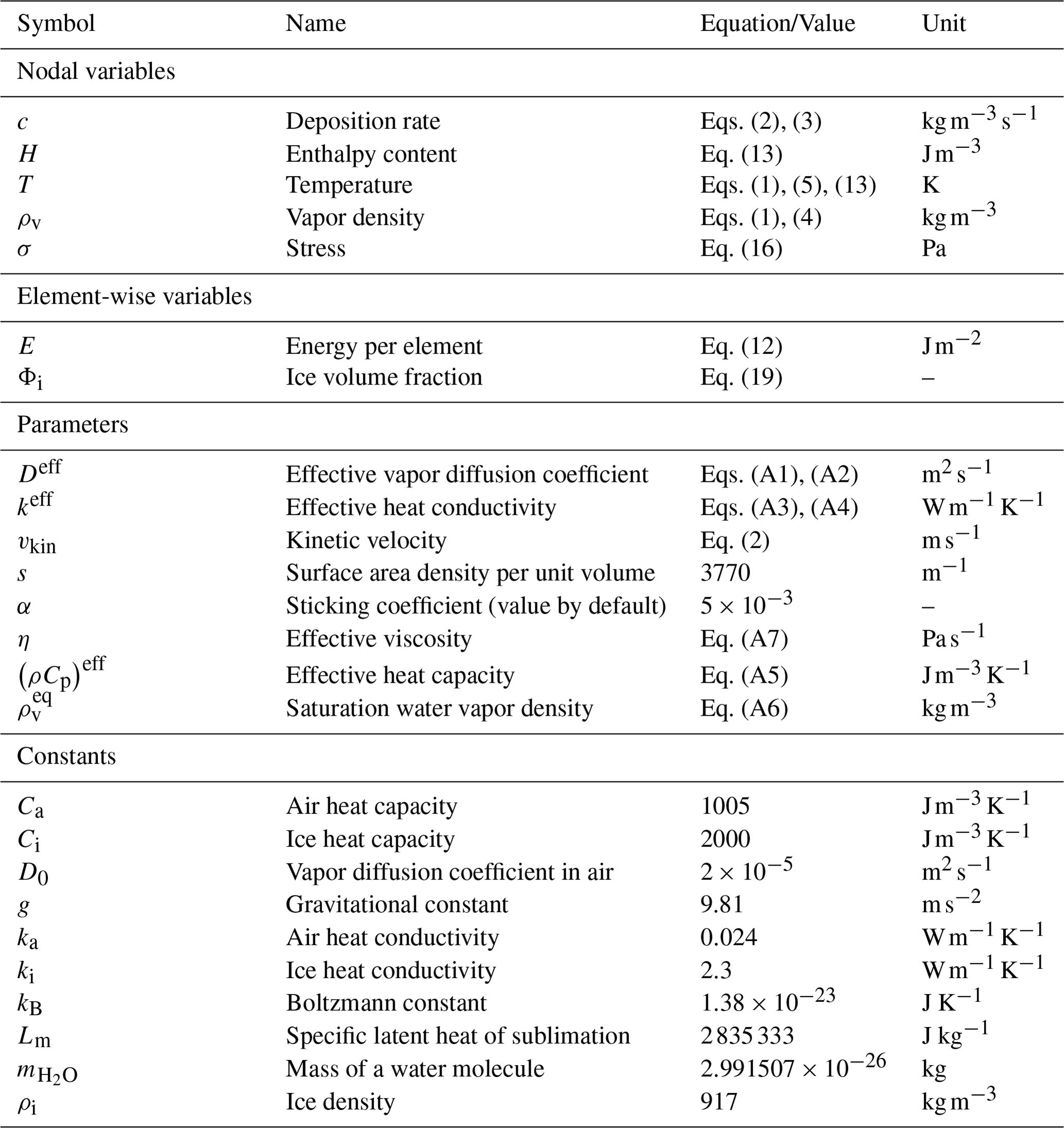
In this section, we go through the most important features of our numerical implementation and underline the main differences compared with the published approaches of Simson et al. (2021) and Schürholt et al. (2022b). All variables, parameters, and constants used in our model are summarized in Table 1.

3.1 Numerical strategy

The spatial discretization of the PDEs of the model is based on the finite-element method (FEM). For the temporal discretization, we use a standard first-order implicit Euler method. Generalities about the FEM and the temporal discretization scheme are presented in Appendix B. This includes a description of the implementation of BCs as well as the calculation of residuals that is necessary to close the energy budget.

3.1.1 Coupling scheme

One of the main goals of our work is to highlight the importance of a coupled numerical solution of the heat and vapor transport processes. Details of the various approaches that have been implemented and compared to reach this conclusion are given in Sect. 3.2. In contrast, the ice mass conservation is systematically solved in a separated step following the same first-order operator-splitting approach as Simson et al. (2021) and Schürholt et al. (2022b). However, as demonstrated in Sect. 2, heat and vapor transfer and deposition are two-way coupled: perturbation of the T and/or ρ_v fields affects the deposition rate field, which in turns changes the distribution of Φ_i; this feeds back on the distributions of the Φ_i-dependent parameters ${\left(\mathit{\rho }{C}_{\mathrm{p}}\right)}^{\mathrm{eff}}$, k^eff and D^eff, impacting the fields of T and ρ_v. Therefore, one has to be aware that solving these two processes sequentially will necessarily introduce some error. Specifically, as the energy and vapor mass budget are solved assuming a constant microstructure, the consecutive modification of the latter through deposition/sublimation breaks the previously computed energy and vapor mass budgets. This results in nonphysical energy and vapor mass sources/sinks that we referred to as energy/mass leakage. However, in most of the natural configurations, the variation in the ice mass related to deposition within targeted time steps in the order of 15 min is expected to remain negligible compared with the total ice mass of the simulated domain. It follows that the energy leakage remains limited, and its associated error in the global energy budget is well identified. Note also that, because our settlement scheme is designed to conserve the ice mass perfectly in the absence of phase change (see Sect. 3.3), there is no such problem of energy leakage for the settlement-induced evolution of Φ_i. For all these reasons, we consider that the operator-splitting approach is acceptable with respect to the ice mass conservation equation.

Figure 1a summarizes the general structure of the model. Within one time step, we first solve the heat and vapor transfer process, which can be modeled using either the system of Calonne or that of Hansen (Fig. 1b). Independently of the considered system, this is done with the distribution of Φ_i from the previous time step. Next, the nodal field of stress is updated from the weight contained in all overlying elements, with the latter being calculated from the distribution of Φ_i from the previous time step. Then, the settlement solver is executed in order to consistently update the mesh node positions and the element-wise field of Φ_i. Finally, a solver is executed to diagnose the amount of energy contained in the domain from the nodal fields of T and ρ_v (for the system of Calonne and the system of Hansen in its T form, i.e., when using T as the prognostic variable) or from the nodal field of enthalpy (for the system of Hansen in its mixed form). At the very end of the time step, the global ice mass and energy budgets are evaluated to check for conservation. Note that any of the solvers can be activated or deactivated depending on the processes of interest. In particular, the settlement-related and deposition-related evolution of Φ_i can easily and independently be switched on or off.

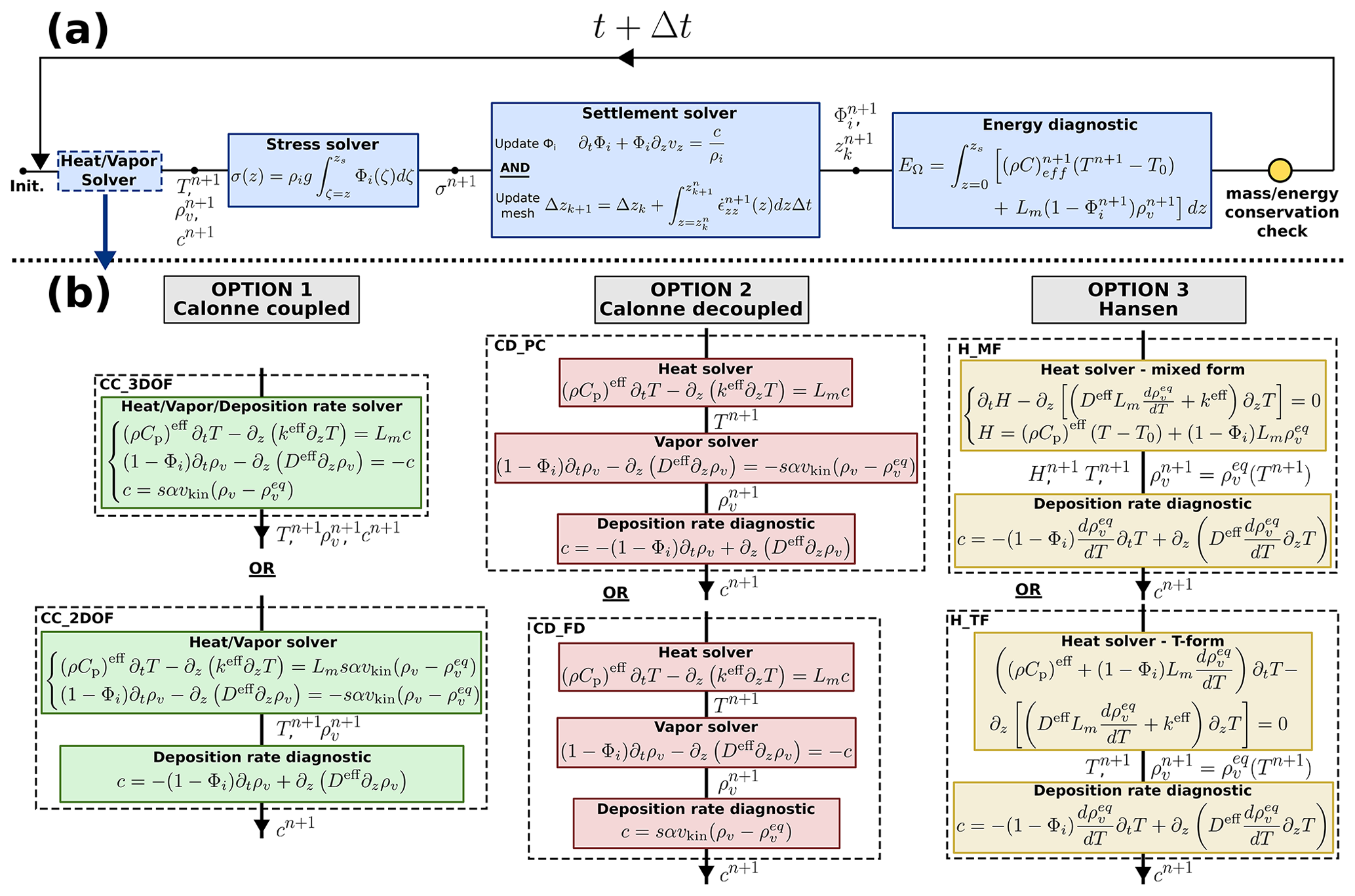
Figure 1 Panel (a) shows the general structure of the model. Panel (b) illustrates the three approaches implemented to compute the fields of temperature, water vapor, and deposition rate for the coupled solution of the Calonne system, the decoupled solution of the Calonne system, and the solution of the Hansen system. For each of these approaches, two strategies have been considered and are described in the text and Appendix C.

3.1.2 Computational domain and notation

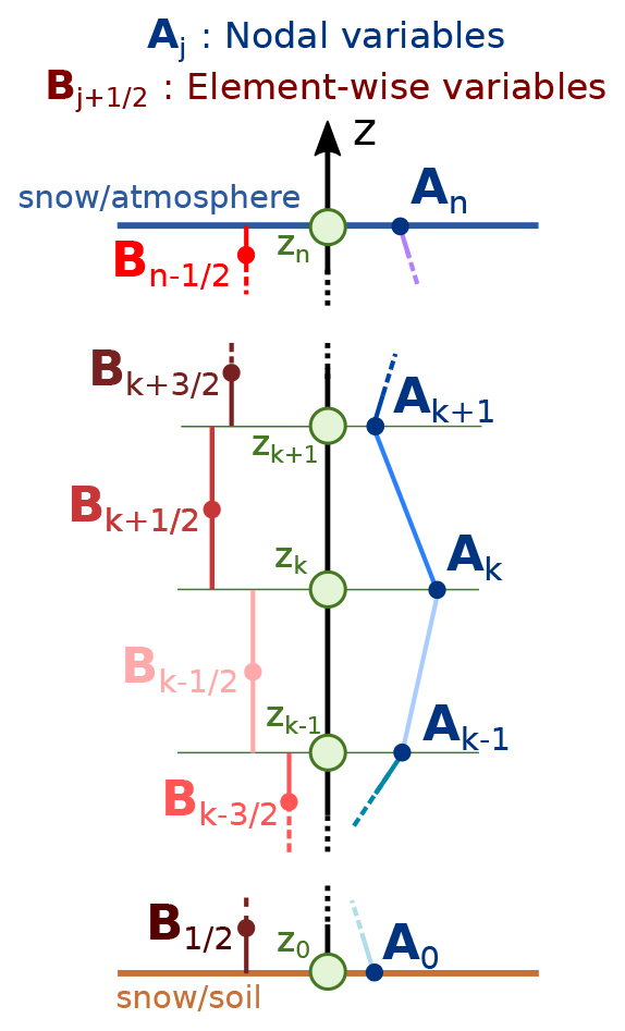
As illustrated in Fig. 2, the snowpack is vertically discretized on a one-dimensional finite-element grid. The z axis is oriented upward, with z=0 corresponding to the soil–snow interface. The initial positions of nodes are based on the user-prescribed initial snowpack height so that the mesh is initially uniform. In the presence of mechanical settlement, the mesh will deform nonuniformly. Note that the application of the FEM to nonuniform mesh is straightforward. In this work, the problem of re-meshing has not been investigated, but it is discussed in Sect. 5. We distinguish between variables defined at nodes and variables defined in an element-wise manner (Table 1). In what follows, the former are identified with the subscripts k, corresponding to the node number, whereas the latter are identified with the subscripts $k+\mathrm{1}/\mathrm{2}$, corresponding to the element number. The element $k+\mathrm{1}/\mathrm{2}$ is located between nodes k and k+1. The total number of nodes is denoted as N_z.

Figure 2 Illustration of the computational domain. The nature of the various model variables is summarized in Table 1.

3.2 Numerical solution of heat and water vapor transfer

3.2.1 Solution of the system of Calonne

As illustrated in Fig. 1b, there are two possible approaches to solve the system of Eqs. (1) and (2): either the whole system can be solved in a coupled way (green boxes in Fig. 1b) or the three equations can be solved sequentially (red boxes in Fig. 1b). Two strategies are investigated for the coupled approach. The first strategy, denoted as CC_3DOF, consists of solving the whole system (Eqs. 1 and 2) at once for the solution vector $\mathit{u}=(T,{\mathit{\rho }}_{\mathrm{v}},c)$. This strategy corresponds to the one adopted by Schürholt et al. (2022b) to treat the Calonne system. The second strategy, denoted as CC_2DOF, consists of injecting Eq. (2) into the right-hand-side terms of Eq. (1) and solving the latter system for the solution vector $\mathit{u}=(T,{\mathit{\rho }}_{\mathrm{v}})$. The c field is then diagnosed from the obtained ρ_v field through the water vapor mass balance equation. Two strategies are also considered for the sequential treatment of the system. In the strategy denoted as CD_PC, the heat equation is solved first with a source term that is fixed from the c field computed at the previous time step. Then, the water vapor mass balance is solved under its diffusion-reaction form: the right-hand side of the equation is replaced by its literal expression (Eq. 2), which introduces a reaction term on ρ_v, while the previously evaluated T field is used to compute the source term stricto sensu, i.e., $s\mathit{\alpha }{v}_{\mathrm{kin}}\left(T\right){\mathit{\rho }}_{\mathrm{v}}^{\mathrm{eq}}\left(T\right)$. Finally, the c field is updated as the closure of the water vapor mass balance from the computed ρ_v field. The second strategy, denoted as CD_FD, is similar to the CD_PC strategy, except that both the heat and water vapor mass balance equations have their right-hand side fixed from the c field computed at the previous time step. The latter is updated in a third step from Eq. (2) using the obtained T and ρ_v fields. The resulting matrix systems are summarized in Appendix C.

In order to manipulate standard mass matrices in which all nonzero terms correspond to the product of test and shape functions, FEM software packages are prone to dealing with a particular form of the heat equation in which the thermal diffusivity $k^{\mathrm{eff}}/{\left(\mathit{\rho }{C}_{\mathrm{p}}\right)}^{\mathrm{eff}}$ is assigned to the flux divergence operator, rather than keeping the heat capacity ${\left(\mathit{\rho }{C}_{\mathrm{p}}\right)}^{\mathrm{eff}}$ as a factor of the accumulation term. Similarly, it can be tempting to divide the water vapor mass balance equation by the factor (1−Φ_i) assigned to the accumulation term in order to deal with the generic form of a diffusion-reaction equation. These operations are performed, for example, in the FEniCS code of Schürholt et al. (2022a). Practically, this corresponds to assigning the inverse of these factors to the stiffness matrix and force vector rather than keeping them in the mass matrix. However, as soon as these factors are nonuniform, which is the case for snow in general as Φ_i=f(z) and ${\left(\mathit{\rho }{C}_{\mathrm{p}}\right)}^{\mathrm{eff}}=f\left({\mathrm{\Phi }}_{\mathrm{i}}\right)$, the conservative forms of Eq. (1) are not equivalent to these reformulations. Therefore, in order to preserve the conservative properties (at given microstructure) of the system of Calonne in the discrete domain, we assign the factors ${\left(\mathit{\rho }{C}_{\mathrm{p}}\right)}^{\mathrm{eff}}$ and (1−Φ_i) directly to the mass matrix (Appendix C). In the following, we refer to this as the proper form of the mass matrix.

By nature, the system of Eq. (1) respects the maximum principle in the continuous domain. From a physical perspective, the maximum principle states that, in the absence of phase change, the maximum value of T (or ρ_v) is reached at either the initial time or at the boundaries (Protter and Weinberger, 2012). In order to get a uniform convergence of the numerical solution to the exact one and avoid nonphysical extrema in the interior of the domain, it can be shown that a discrete counterpart of this principle, the so-called discrete maximum principle (DMP), must be fulfilled (Ciarlet, 1973). However, in some situations, the FEM is inclined to violate the DMP due to, among others, the treatment of time derivatives (e.g., Celia et al., 1990) and/or of reaction terms (e.g., John and Schmeyer, 2008). A sufficient condition for the DMP to be respected is that the matrix A of the system (Eq. B2) has the following properties: (i) all diagonal terms are positive, (ii) all off-diagonal terms are negative or zero, and (iii) the row sums are positive (John and Schmeyer, 2008). Thus, a commonly used method to enforce the matrix system to satisfy the DMP without adding further constraints on the time step is to lump the mass matrix and/or the reactive part of the stiffness matrix. This operation consists of replacing the diagonal term in each row of the considered matrix with the sum of all terms in the row while all off-diagonal terms are simultaneously forced to zero (e.g., Milly, 1985; Celia et al., 1990; John and Schmeyer, 2008; Thomée, 2015). In the present work, this method is adopted whenever spurious oscillations show up. As we will show, although the obtained solution fields are very slightly modified, this method enables the removal of spurious oscillations without affecting energy conservation.

As mentioned in Sect. 2.1, the nonlinearity of the system of Calonne is related to the dependence of the source terms, through the parameters ${\mathit{\rho }}_{\mathrm{v}}^{\mathrm{eq}}$ and v_kin, on temperature (Appendix A4). As a consequence, this nonlinearity vanishes whenever these parameters are computed from a T field obtained in a separated step. This is the case for both strategies based on the decoupled solution for the system. In contrast, as soon as a coupled solution of the system is considered, a linearization procedure is required. For both strategies of the coupled approach, we implement a linearization algorithm which mixes a Picard method for v_kin and a Newton method for ${\mathit{\rho }}_{\mathrm{v}}^{\mathrm{eq}}$. Practically, when solving the system (Eq. B2) at iteration k+1 for u^k+1, the value of $v_{\mathrm{kin}}^{k+\mathrm{1}}$ is fixed using the temperature field obtained at previous iteration, i.e., $v_{\mathrm{kin}}^{k+\mathrm{1}}=v_{\mathrm{kin}}\left(T^k\right)$. Within the same iteration step, the value of ${\mathit{\rho }}_{\mathrm{v}}^{\mathrm{eq},k+\mathrm{1}}$ is evaluated as follows:

$$\begin{array}{}\text{(8)}& {\mathit{\rho }}_{\mathrm{v}}^{\mathrm{eq},k+\mathrm{1}}={\left.{\displaystyle \frac{\mathrm{d}{\mathit{\rho }}_{\mathrm{v}}^{\mathrm{eq}}}{\mathrm{d}T}}\right|}_{T=T^k}(T^{k+\mathrm{1}}-T^k)+{\mathit{\rho }}_{\mathrm{v}}^{\mathrm{eq}}\left(T^k\right).\end{array}$$

The first iteration corresponds to the solution vector obtained at the previous time step Tⁿ. The convergence criterion of the linearization algorithm reads as follows:

$$\begin{array}{}\text{(9)}& \mathrm{2}{\displaystyle \frac{\left|\left|{\mathit{u}}^{k+\mathrm{1}}\right|-\left|{\mathit{u}}^k\right|\right|}{\left|{\mathit{u}}^{k+\mathrm{1}}\right|+\left|{\mathit{u}}^k\right|}}<\mathit{\epsilon },\end{array}$$

where the tolerance criterion is set to $\mathit{\epsilon }={\mathrm{10}}^{-\mathrm{5}}$ by default. This convergence criterion corresponds to the one adopted by default in the open-source Elmer multi-physics finite-element code (https://www.csc.fi/web/elmer, last access: 25 September 2023). Among many other applications, Elmer is one of the most popular codes for numerical simulations in the field of glaciology (Gagliardini et al., 2013). A number of other measures of the change in the solution between two consecutive iterations could be used instead of Eq. (9). We stress that the convergence criterion is used only to stop the nonlinear iterations, it has no impact on the intermediate iterations. In all simulations that are presented in Sect. 4, the systems at stake are not strongly nonlinear and only one to three nonlinear iterations are needed to satisfy the convergence criterion. Most importantly, the convergence is smooth, and the solution is already very close to its final (converged) value after the first nonlinear iteration (i.e., the change in the solution between, e.g., iterations one and two are very small compared with the change between the first guess and iteration one). It follows that the obtained solution fields are unlikely to show significant sensitivity to the formulation of the convergence criterion for the numerical experiments presented in this study. This point has been confirmed by dedicated sensitivity tests (not shown in this paper).

Once the linearization algorithm has converged, the residuals of the system are evaluated to assess the sensible heat $\mathrm{\Delta }t{\mathit{F}}_{\mathrm{T}}^{\partial \mathrm{\Gamma }}$ and water vapor mass $\mathrm{\Delta }t{\mathit{F}}_{\mathrm{P}}^{\partial \mathrm{\Gamma }}$ that have entered or left the domain over the time step. The energy budget is evaluated at the very end of the time step by comparing the evolution of the energy contained in the domain since the previous time step ΔE_Ω to the aforementioned boundary fluxes. In practice, we compute the following:

$$\begin{array}{}\text{(10)}& E_{\mathrm{leak}}=\mathrm{\Delta }{E}_{\mathrm{\Omega }}-\mathrm{\Delta }t({\mathit{F}}_{\mathrm{T}}^{\partial \mathrm{\Gamma }}+L_{\mathrm{m}}{\mathit{F}}_{\mathrm{P}}^{\partial \mathrm{\Gamma }})-\mathrm{\Delta }t{L}_{\mathrm{m}}{F}_{\mathrm{P},\mathrm{set}.}^{\partial \mathrm{\Gamma }},\end{array}$$

where E_leak is the energy leakage, which is zero if energy is conserved. As mentioned in Sect. 2, because the contribution of dry air in the effective heat capacity of snow is neglected, the dry air expelled from the snowpack in response to settlement does not affect the energy budget. On the contrary, the latent energy loss due to water vapor leaving the domain as the snowpack settles must be accounted for through the term $\mathrm{\Delta }t{L}_{\mathrm{m}}{F}_{\mathrm{P},\mathrm{set}.}^{\partial \mathrm{\Gamma }}$. The water vapor mass leaving the snowpack over Δt is diagnosed in the settlement solver as follows:

$$\begin{array}{}\text{(11)}& \mathrm{\Delta }t{F}_{\mathrm{P},\mathrm{set}.}^{\partial \mathrm{\Gamma }}=\sum _{k=\mathrm{1}}^{N_{z-\mathrm{1}}}\left[\underset{\mathit{\zeta }=z_k^n}{\overset{z_{k+\mathrm{1}}^n}{\int }}{\mathit{\rho }}_{\mathrm{v}}^{n+\mathrm{1}}\mathrm{d}\mathit{\zeta }-\underset{\mathit{\zeta }=z_k^{n+\mathrm{1}}}{\overset{z_{k+\mathrm{1}}^{n+\mathrm{1}}}{\int }}{\mathit{\rho }}_{\mathrm{v}}^{n+\mathrm{1}}\mathrm{d}\mathit{\zeta }\right].\end{array}$$

The total energy contained in the domain E_Ω is diagnosed as the sum of the energies contained in each element in the last executed solver (Fig. 1a). The energy contained in the element $k+\mathrm{1}/\mathrm{2}$ is calculated as follows:

$$\begin{array}{}\text{(12)}& \begin{array}{rl}{E}_{k+\mathrm{1}/\mathrm{2}}& =\underset{\mathit{\zeta }=z_k^{n+\mathrm{1}}}{\overset{z_{k+\mathrm{1}}^{n+\mathrm{1}}}{\int }}\left[\left(\mathit{\rho }C{)}_{\mathrm{eff}}^{n+\mathrm{1}}\right(T^{n+\mathrm{1}}-T_{\mathrm{0}})\right.\\ & \left.+L_{\mathrm{m}}(\mathrm{1}-{\mathrm{\Phi }}_{\mathrm{i}}^{n+\mathrm{1}}){\mathit{\rho }}_{\mathrm{v}}^{n+\mathrm{1}}\right]\mathrm{d}\mathit{\zeta },\end{array}\end{array}$$

where T₀ is an arbitrary reference temperature, which we set to T₀=273 K.

3.2.2 Solution of the system of Hansen

For the system of Hansen, two implementation strategies are also investigated (yellow boxes in Fig. 1b). In the first strategy, denoted as H_MF, the prognostic equation that relates to T evolution is treated using its mixed form. Concretely, this consists of solving the following system for the solution vector $\mathit{u}=(H,T)$:

$$\begin{array}{}\text{(13)}& \left\{\begin{array}{l}{\partial }_{t}H-{\partial }_z\left[\left(D^{\mathrm{eff}}{L}_{\mathrm{m}}\frac{\mathrm{d}{\mathit{\rho }}_{\mathrm{v}}^{\mathrm{eq}}}{\mathrm{d}T}+k^{\mathrm{eff}}\right){\partial }_{z}T\right]=\mathrm{0}\\ H={\left(\mathit{\rho }{C}_{\mathrm{p}}\right)}^{\mathrm{eff}}\left(T-T_{\mathrm{0}}\right)+(\mathrm{1}-{\mathrm{\Phi }}_{\mathrm{i}})L_{\mathrm{m}}{\mathit{\rho }}_{\mathrm{v}}^{\mathrm{eq}},\end{array}\right.\end{array}$$

where H is the enthalpy content defined as a nodal variable. Because H is a Φ_i-dependent prognostic variable, it must be updated within the settlement solver after Φ_i has been updated. In order to illustrate the problem of violation of energy conservation when a chain rule is performed in the discrete domain (Sect. 2.2), we consider a second strategy, denoted as H_TF, which consists of solving the prognostic equation of the Hansen system using its usual T form (Eq. 5). The resulting matrix systems are summarized in Appendix C. The H_TF strategy is the one adopted by Simson et al. (2021) and Schürholt et al. (2022b). Independently of the chosen strategy, the field of ρ_v is deduced from the obtained T field assuming that water vapor density is saturated everywhere. Then, the second equation of (Eq. 3) is solved for the field of c.

For the T form of the prognostic equation, we are careful to assign the apparent heat capacity directly to the mass matrix (proper form of the mass matrix). Note that ambiguities do not arise for the mixed form of the equation, as it does not include any multiplying factor in the accumulation term. Furthermore, as for the Calonne system, spurious oscillations related to the violation of the DMP can occur. Again, this difficulty is overcome by lumping the mass matrices of both the prognostic equation that relates to T evolution (or H evolution for the mixed form) and the diagnostic equation of c when necessary. As mentioned in Sect. 2.2, both the mixed form and T form of the prognostic equation are nonlinear due to the dependence of $\mathrm{d}{\mathit{\rho }}_{\mathrm{v}}^{\mathrm{eq}}/\mathrm{d}T$ on T (Appendix A4). This nonlinearity is treated via the implementation of a Picard linearization loop. As for the coupled Calonne system, the tolerance criterion is set to $\mathit{\epsilon }={\mathrm{10}}^{-\mathrm{5}}$ by default. Note that the approach of Simson et al. (2021), which consists of linearizing the equation by fixing the value of $\mathrm{d}{\mathit{\rho }}_{\mathrm{v}}^{\mathrm{eq}}/\mathrm{d}T$ from the T field obtained at the previous time step, is equivalent to performing a single Picard iteration. In this case, the obtained solution does not correspond to the implicit solution of the problem and, thus, does not necessarily possess its stability features.

As for the Calonne system, the residuals are evaluated immediately after the convergence of the linearization algorithm. Note that, because the Hansen system contains only one prognostic equation that mixes up the contributions of latent and sensible heat to the energy budget, the obtained residuals correspond to the total enthalpy fluxes at boundaries, without any reference to how these fluxes are split between sensible and latent heat fluxes. Again, these boundary fluxes are used to close the energy budget. The total energy contained in the domain is directly obtained through integration of the nodal enthalpy over the elements for the mixed-form case. For the T-form case, it is evaluated from T based on Eq. (12) using the assumption of saturated water vapor density. As for the Calonne system, the energy budget accounts for energy loss related to the water vapor mass leaving the snowpack when settlement is activated through Eq. (11).

Although the c field is diagnosed a posteriori from the obtained T field based on the second equation of Eq. (3), this solution is also based on the FEM, and a boundary flux term naturally appears in the force vector through integration by parts of the divergence operator. In the absence of any prescription from the user, the natural BC applies and this term is forced to be zero. However, the existence of a boundary flux strongly affects the deposition rate at the corresponding boundary node, as the local oversaturation/undersaturation governs the magnitude of the deposition/sublimation that is necessary to maintain vapor saturation. It follows that the prescription of proper vapor fluxes at boundaries is an integral part of the physical problem and should ideally arise from a vapor budget at interfaces, similarly to the standard surface energy budget. On the other hand, fixing c to an arbitrary value at boundaries (Dirichlet type BCs), as done by Simson et al. (2021), implicitly implies the prescription of a water vapor mass flux that adjusts itself so that saturation is maintained with a fixed contribution of deposition/sublimation. This boundary vapor flux then corresponds to the residuals of the vapor mass budget equation. This topic is further explored in Sect. 4.6.

3.3 A mass-conservative Lagrangian settlement scheme

3.3.1 General considerations

Our settlement scheme is based on the method of characteristics as presented in Simson et al. (2021) with some corrections to guarantee ice mass conservation as well as a more explicit formulation of the element-wise nature of this conservation. The general idea of this approach is that the mesh nodes should move at the velocity of the ice matrix as the latter settles so that all ice mass fluxes related to settlement wipe out in the working frame, thereby resorting to a Lagrangian coordinate system. Concretely, this allows for the elimination of the advection term v⋅∇Φ_i from the continuity equation, which is then in one dimension:

$$\begin{array}{}\text{(14)}& {\partial }_t{\mathrm{\Phi }}_{\mathrm{i}}+{\mathrm{\Phi }}_{\mathrm{i}}{\partial }_z{v}_z={\displaystyle \frac{c}{{\mathit{\rho }}_{\mathrm{i}}}},\end{array}$$

where ∂_zv_z is the divergence of the settling velocity which, in one dimension, directly corresponds to the vertical strain rate ${\dot{\mathit{ϵ}}}_{zz}$. The vertical strain rate relates to the vertical stress σ_zz through the constitutive law of snow, which we take as a simple linear viscous law:

$$\begin{array}{}\text{(15)}& {\dot{\mathit{ϵ}}}_{zz}={\displaystyle \frac{\mathrm{1}}{\mathit{\eta }}}{\mathit{\sigma }}_{zz},\end{array}$$

where η is the effective viscosity of snow and σ_zz is the vertical stress. The effective viscosity is an important and poorly constrained snow property that depends, among others, on microstructure and temperature (e.g., Wiese and Schneebeli, 2017). Here, we use the viscosity parameterization of Vionnet et al. (2012) where the viscosity increases exponentially with density and decreases exponentially with temperature according to Eq. (A7). Note that Simson et al. (2021) also considered the case of a nonlinear Glen's flow law as well as the case of a constant viscosity. As the goal of this study is not an assessment of the model sensitivity to parameterization choices but rather to the details of the numerical treatment of the equations, we do not consider these cases here. Neglecting the contribution of air in the effective density of snow, the momentum conservation equation relates the distribution of the vertical stress to that of the ice volume fraction as follows:

$$\begin{array}{}\text{(16)}& {\partial }_z{\mathit{\sigma }}_{zz}={\mathit{\rho }}_{\mathrm{i}}g{\mathrm{\Phi }}_{\mathrm{i}}\left(z\right),\end{array}$$

where g is gravity.

As underlined by Simson et al. (2021), Eq. (14) and its Lagrangian perspective corresponds to the strategy employed in all available detailed snowpack models to represent settlement, although it is usually not explicitly stated. Concretely, the constitutive law of snow is used to relate the stress supported by a layer, calculated as the cumulative weight of all overlying layers, to its total deformation. This total deformation is then used to either directly update the layer thickness defined as a state variable (e.g., Jordan, 1991; Vionnet et al., 2012) or to update the mesh coordinates using the fact that the node at the soil–snow interface does not move (e.g., Bader and Weilenmann, 1992; Bartelt and Lehning, 2002). The effective density, defined as a layer property, is then simply updated so that, in the absence of phase change, the mass contained within each layer remains the same before and after settlement. The layer-based nature of this scheme is obvious, in that conservation is not fulfilled locally but rather on average over finite space intervals referred to as control volumes (e.g., Jordan, 1991), elements (e.g., this study, Bartelt and Lehning, 2002), or layers (e.g., Bader and Weilenmann, 1992; Bartelt and Lehning, 2002; Vionnet et al., 2012), depending on the numerical method chosen to solve the other PDEs of the model. In contrast, as Eq. (14) expresses the local ice mass conservation, one may assume that its actual solution would enable a switch from this traditional layer-based vision to a more continuous description of the snowpack. We stress that this impression relies on a confusion between numerical and physical layers. Indeed, although all physical quantities involved in Eqs. (14)–(16) are continuous functions of z and can be calculated anywhere in the continuous domain, as soon as we go through the necessary numerical discretization step, the continuous vision breaks and we step back to a discrete description in which the ice phase is conserved on average over finite space intervals that can be seen as numerical layers. The settlement scheme then consists of two numerical operations that must be done in parallel and in a consistent way to ensure that conservative properties of Eq. (14) are preserved: (i) the update of the mesh node positions so that the variation in the mass contained in each element over one time step is entirely due to phase change and not at all to settlement and (ii) the update of the ice volume fraction defined as an element-wise state variable accounting for the possible source term due to phase change.

3.3.2 Update of mesh node positions

The displacement Δz_k+1 of node k+1 between t and t+Δt corresponds to the displacement Δz_k of the underlying node k to which the total deformation of the space interval between k and k+1 over Δt must be added. This condition can be written as follows:

$$\begin{array}{}\text{(17)}& \mathrm{\Delta }{z}_{k+\mathrm{1}}=\mathrm{\Delta }{z}_k+\underset{z_k^n}{\overset{z_{k+\mathrm{1}}^n}{\int }}{\dot{\mathit{ϵ}}}_{zz}^{n+\mathrm{1}}\left(z\right)\mathrm{d}z\mathrm{\Delta }t,\end{array}$$

where ${\dot{\mathit{ϵ}}}_{zz}^{n+\mathrm{1}}$ is the vertical strain rate that, in one dimension, directly corresponds to the divergence of the vertical velocity field ∂_zv_z. By exploiting the fact that the node located at the soil–snow interface is immobile, we can trace the displacement of all nodes of the domain through Eq. (17). A difficulty arises in the numerical treatment of the integral term of Eq. (17) after spatial discretization. Indeed, the numerical integration requires an assumption regarding the spatial variation in the integrand in between nodes. While this assumption is made a priori via the choice of the shape functions in the FEM, only the nodal values of the fields are considered to constitute the solution in the finite-difference method employed by Simson et al. (2021), without any explicit reference to how these fields should vary between nodes (Patankar, 1980). In their mesh deformation procedure, Simson et al. (2021) do not directly use the strain rate ${\dot{\mathit{ϵ}}}_{zz}$ to evaluate the total deformation of the space intervals in between nodes; rather, they perform a numerical integration to recover the settling velocity v_z and use the latter to move the nodes. A careful inspection of Eq. (17) of Simson et al. (2021) reveals that this numerical integration implicitly assumes that the strain rate calculated at node k from the stress and viscosity evaluated at node k actually applies to the whole space interval between the node k and the node k−1 (assuming that the $\mathrm{\Delta }{z}_j^n=z_{j+\mathrm{1}}^n-z_j^n$ stated in Eq. 17 of Simson et al., 2021, actually means $\mathrm{\Delta }{z}_j^n=z_j^n-z_{j-\mathrm{1}}^n$, which makes more sense and is in accordance with their published code). Similarly, the numerical integration of the momentum conservation equation yielding the nodal stresses from the distribution of Φ_i as expressed in Eq. (18) of Simson et al. (2021) implicitly assumes that the value of Φ_i stored at node k actually applies to the whole space interval between nodes k and k+1. In other words, in the approach of Simson et al. (2021), the distribution of Φ_i is piecewise constant over numerical layers, but the information is only assigned to the bottom node of the considered numerical layer. As detailed in Appendix D1, the fact that Φ_i at node k relates to the snow mass contained between nodes k and k+1, whereas the strain rate calculated at node k is used to deform the space interval between nodes k and k−1, leads to an inconsistency that hampers mass conservation.

In contrast, in our approach, Φ_i is defined in an element-wise manner, whereas the stress is a nodal variable. The latter is calculated at each node k as the cumulative weight of all overlying elements:

$$\begin{array}{}\text{(18)}& {\mathit{\sigma }}_{zz,k}^{n+\mathrm{1}}=\sum _{j=k}^{N_z-\mathrm{1}}g{\mathrm{\Phi }}_{\mathrm{i},j+\mathrm{1}/\mathrm{2}}^n{\mathit{\rho }}_{\mathrm{i}}(z_{j+\mathrm{1}}^n-z_j^n).\end{array}$$

This equation is formally equivalent to Eq. (18) of Simson et al. (2021) except that ${\mathrm{\Phi }}_{\mathrm{i},j+\mathrm{1}/\mathrm{2}}$ explicitly corresponds to an averaged quantity applying to the whole element $j+\mathrm{1}/\mathrm{2}$ between nodes j and j+1. The motion of all nodes can then be determined directly by solving Eq. (17) where the integral term is treated through the Gaussian quadratures.

3.3.3 Update of ice volume fraction

It can be shown that conservation of the ice mass is guaranteed only if the temporal discretization of Eq. (14) is based on an implicit numerical scheme (Appendix E). Therefore, in our approach, we replace the first-order Euler explicit temporal discretization given in Eq. (15) of Simson et al. (2021) with the following:

$$\begin{array}{}\text{(19)}& {\mathrm{\Phi }}_{\mathrm{i},k+\mathrm{1}/\mathrm{2}}^{n+\mathrm{1}}={\displaystyle \frac{{\mathrm{\Phi }}_{\mathrm{i},k+\mathrm{1}/\mathrm{2}}^n+\mathrm{\Delta }t\frac{c_{k+\mathrm{1}/\mathrm{2}}^{n+\mathrm{1}}}{{\mathit{\rho }}_{\mathrm{i}}}}{\mathrm{1}+\mathrm{\Delta }t{\dot{\mathit{ϵ}}}_{zz,k+\mathrm{1}/\mathrm{2}}^{n+\mathrm{1}}}},\end{array}$$

where the mean strain rate ${\dot{\mathit{ϵ}}}_{zz,k+\mathrm{1}/\mathrm{2}}^{n+\mathrm{1}}$ and mean deposition rate $c_{k+\mathrm{1}/\mathrm{2}}^{n+\mathrm{1}}$ of element $k+\mathrm{1}/\mathrm{2}$ are calculated as the integral of the corresponding field over the element using Gaussian quadratures divided by the length of the considered element before deformation.

4 Numerical simulations

In this section, we compare the capabilities of the various numerical treatments introduced above to provide solutions to the coupled problem of heat transport, vapor transport, and settlement in snow that are stable, accurate, and respect energy and mass conservation. To this end, we use some of the experiments proposed by Schürholt et al. (2022b) and Simson et al. (2021) as numerical benchmarks. The main features of the numerical setup and model configurations of all experiments described in the following are summarized in Table 2. All simulations are run with the parameterization (Eq. A6) for the saturation vapor density and with the Calonne parameterizations of effective parameters (given by Eqs. A1–A3), unless stated otherwise. Note that the Hansen parameterizations of effective parameters given by Eqs. (A2)–(A4) have also been implemented. In what follows, we use the absolute root-mean-square deviations (RMSDs) as a metric when comparing two solution fields produced with two different implementations. For interpretation, it is important to relate these RMSDs to the typical orders of magnitude of the considered fields shown in respective figures.

Table 2 Summary of numerical setups and model configurations. Scenarios 2 and 3 are taken from Schürholt et al. (2022b). Cases 6 and 7 are taken from Simson et al. (2021). Dirichlet BCs for T are T₀=273 K and T_h=253 K. Dirichlet BCs for ρ_v are ${\mathit{\rho }}_{\mathrm{v},\mathrm{0}}={\mathit{\rho }}_{\mathrm{v}}^{\mathrm{eq}}\left(T_{\mathrm{0}}\right)$ and ${\mathit{\rho }}_{\mathrm{v},h}={\mathit{\rho }}_{\mathrm{v}}^{\mathrm{eq}}\left(T_h\right)$.

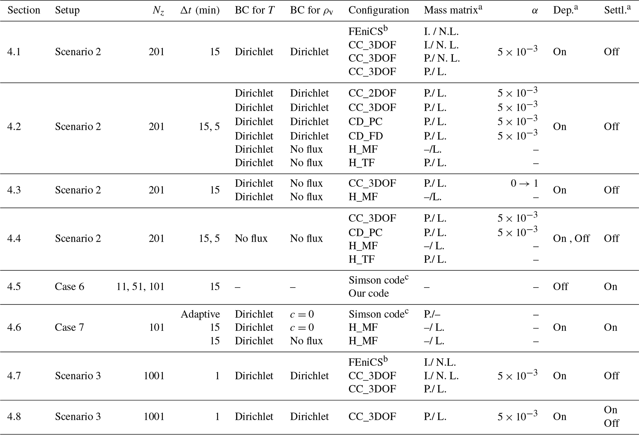
^a The following abbreviations are used in the table: I. – improper (Sect. 3.2); P. – proper (Sect. 3.2); N.L. – not lumped (Sect. 3.2); L. – lumped (Sect. 3.2); Dep. – deposition; and Settl – settlement. ^b Code of Schürholt et al. (2022a). ^c Code of Simson and Kowalski (2021).

4.1 On the form of the mass matrices

In this part, we reproduce Scenario 2 presented in Schürholt et al. (2022b) to illustrate the importance of dealing with proper mass matrices. Concretely, we consider a 1 m thick snowpack with a piecewise linear initial density profile mimicking a stratified snowpack containing a crust as well as an ice layer at the bottom (Eq. 16 of Schürholt et al., 2022b). All BCs are Dirichlet-type conditions and are constant over time: the bottom and top temperatures are fixed to T₀=273 K and T_h=253 K, respectively, while the bottom and top water vapor densities are set assuming saturation at boundaries, i.e., ${\mathit{\rho }}_{\mathrm{v},\mathrm{0}}={\mathit{\rho }}_{\mathrm{v}}^{\mathrm{eq}}\left(T_{\mathrm{0}}\right)$ and ${\mathit{\rho }}_{\mathrm{v},h}={\mathit{\rho }}_{\mathrm{v}}^{\mathrm{eq}}\left(T_h\right)$. The initial temperature profile is linear between boundary values, and the initial water vapor density profile is deduced from the latter assuming that the water vapor density is initially saturated (solid black lines in Fig. 3). To facilitate a comparison with results presented by Schürholt et al. (2022b), all simulations described in this part are run with settlement deactivated and deposition feedback on Φ_i activated. The time step is set to Δt=15 min. The mesh is uniform and contains 200 elements. For the simulations with the Calonne model, the sticking coefficient is set to a default value of $\mathit{\alpha }=\mathrm{5}\times {\mathrm{10}}^{-\mathrm{3}}$ so that our sαv_kin is comparable to the ${\mathit{\rho }}_{\mathrm{i}}s/\mathit{\beta }{\mathit{\rho }}_{\mathrm{v}}^{\mathrm{eq}}$ adopted by Schürholt et al. (2022b).

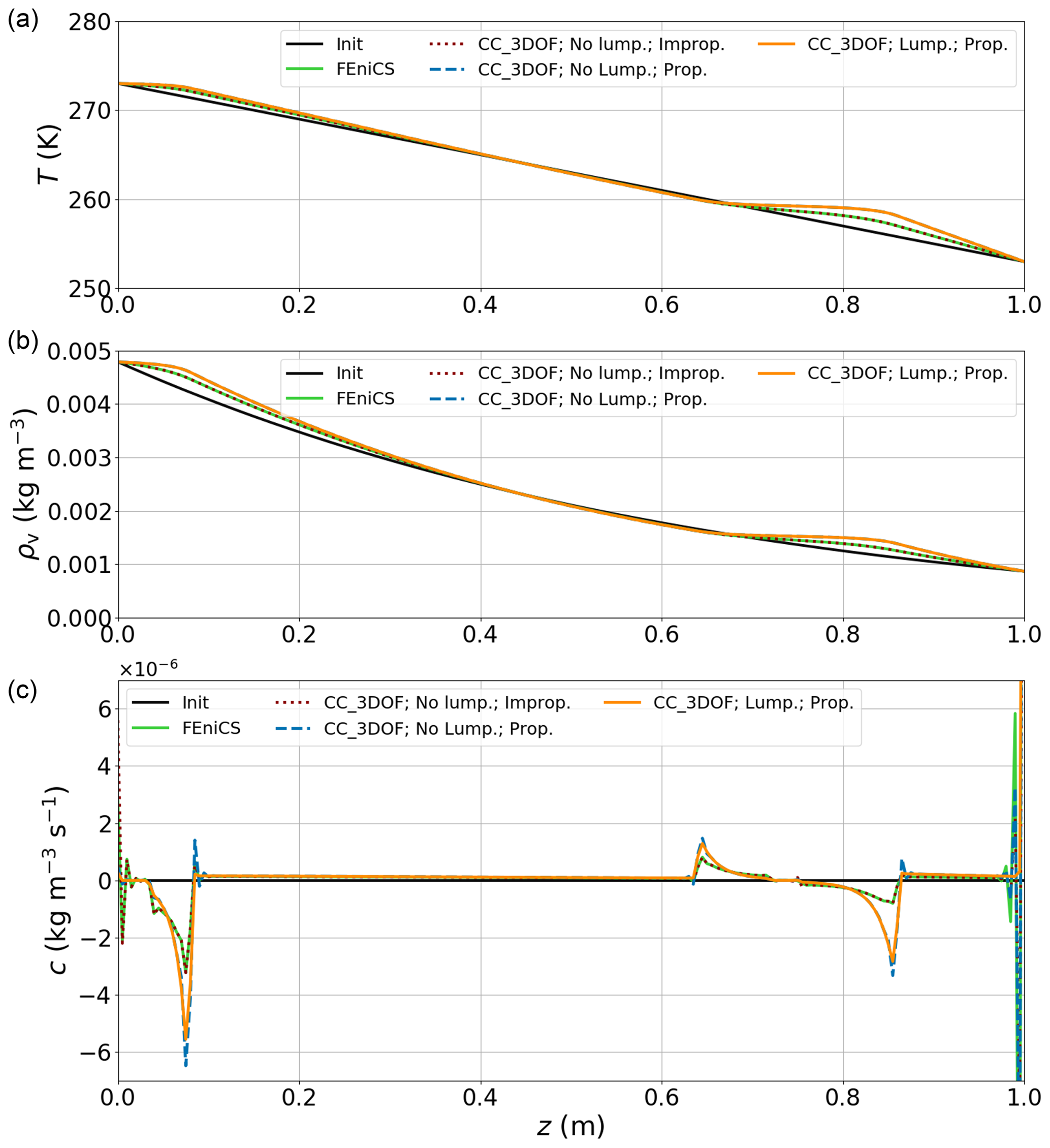
Figure 3 Comparison of temperature (a), water vapor density (b), and deposition rate (c) fields produced by FEniCS, CC_3DOF without lumping and with the improper mass matrix, CC_3DOF without lumping but with the proper mass matrix, and CC_3DOF with lumping and the proper mass matrix after 38 h of simulation for Scenario 2 of Schürholt et al. (2022b). The dashed blue and solid orange lines are superimposed in panels (a) and (b). The solid black lines correspond to the initial conditions.

Figure 3 shows the vertical profiles of temperature, vapor density, and deposition rate produced after 38 h of simulation by FEniCS and by different versions of CC_3DOF. The FEniCS run is based on the code of Schürholt et al. (2022a), with slight adaptations. In particular, the original Crank–Nicolson time scheme adopted by Schürholt et al. (2022b) is replaced by a fully implicit scheme. Despite slight differences in the numerical implementation (e.g., Φ_i is a nodal variable in FEniCS and an element-wise variable in our model, variable-dependent parameters are evaluated at nodes in FEniCS and directly at Gaussian points in our model, and the expressions of the source terms are not strictly equivalent in FEniCS and in our model), the solution fields produced by FEniCS are very close to those obtained with CC_3DOF when the mass matrix has the improper form and no lumping is performed (superimposed solid green and dotted red lines). This can be quantified by calculating the RMSDs between the solutions obtained with the two approaches: it is $\mathrm{3.7}\times {\mathrm{10}}^{-\mathrm{4}}$ K for T and $\mathrm{4.4}\times {\mathrm{10}}^{-\mathrm{8}}$ kg m⁻³ for ρ_v. A more noticeable difference is found with respect to the amplitude of the oscillations occurring on the field of c at the top boundary of the domain. Note that oscillations are also observed at the bottom boundary of the domain as well as at the boundaries of the deposition/sublimation peaks, but they are of similar amplitude in both approaches, except at the very bottom node. Thus, the RMSD between the fields of c produced by the two approaches is $\mathrm{3.7}\times {\mathrm{10}}^{-\mathrm{6}}$ $\mathrm{kg}{\mathrm{m}}^{-\mathrm{3}}{\mathrm{s}}^{-\mathrm{1}}$ when the whole domain is considered, whereas it is reduced to $\mathrm{2.4}\times {\mathrm{10}}^{-\mathrm{8}}$ $\mathrm{kg}{\mathrm{m}}^{-\mathrm{3}}{\mathrm{s}}^{-\mathrm{1}}$ when the first bottom node and four top nodes are omitted.

In contrast, adopting the proper form of the mass matrix significantly changes the T and ρ_v fields in places where peaks in sublimation/deposition are observed (dashed blue lines hidden below the solid orange lines in Fig. 3a and b): the RMSDs between the solution fields of T and ρ_v obtained with CC_3DOF using the improper mass matrix and those obtained with CC_3DOF using the proper mass matrix are increased to 0.42 K and $\mathrm{6.5}\times {\mathrm{10}}^{-\mathrm{5}}$ kg m⁻³, respectively. The sublimation/deposition peaks also become sharper (dashed blue line in Fig. 3c). The oscillations are mostly reproduced, with larger amplitudes at deposition/sublimation peaks and smaller amplitudes at domain boundaries, especially at the bottom boundary. These spurious oscillations are related to the violation of the DMP. Note that oscillations of the same nature also occur when FEniCS is run with a Crank–Nicolson time scheme (not shown). As expected, these oscillations vanish when the mass matrix is lumped (solid orange line in Fig. 3).

4.2 On the different solver options

Here, we use the same numerical setup as above in order to compare the relative performance of the various numerical treatments of the Calonne system that are summarized in Fig. 1b. All simulations are run with the proper form of the mass matrices and with lumping activated. In addition to the time step of Δt=15 min, all simulations are also run with a time step reduced to Δt=5 min. A first important result is that the boundary values taken by the field of c depart strongly from their distribution in the interior of the domain and that they are highly sensitive to the chosen numerical approach (Fig. 4c). This topic is treated in detail in Sect. 4.6. Secondly, it turns out that the two strategies investigated for the coupled solution of the Calonne system, i.e., CC_2DOF and CC_3DOF, produce solution fields that are very close. After 24 h of simulation with Δt=15 min, the RMSDs for the T, ρ_v, and c fields produced with the two methods amount to $\mathrm{1.8}\times {\mathrm{10}}^{-\mathrm{4}}$ K, $\mathrm{1.6}\times {\mathrm{10}}^{-\mathrm{8}}$ kg m⁻³, and $\mathrm{1.2}\times {\mathrm{10}}^{-\mathrm{6}}$ $\mathrm{kg}{\mathrm{m}}^{-\mathrm{3}}{\mathrm{s}}^{-\mathrm{1}}$, respectively. The higher (relative) deviation in c is mostly due to the values obtained at the two boundary nodes, which are slightly sensitive to the chosen strategy: if the very top and bottom nodes are omitted, the RMSD for the c field is reduced to $\mathrm{3.7}\times {\mathrm{10}}^{-\mathrm{9}}$ $\mathrm{kg}{\mathrm{m}}^{-\mathrm{3}}{\mathrm{s}}^{-\mathrm{1}}$. In addition, the solution fields produced by CC_2DOF and CC_3DOF show very little sensitivity to the time step size (superimposed green and blue lines in Fig. 4) with similar RMSDs as above for all three fields when Δt=5 min. In contrast, the decoupled solution of the Calonne system leads to significantly different behaviors. First, the CD_FD approach is highly unstable, with the ρ_v and T fields rapidly diverging towards unrealistic values. This continues to be the case even when the time step size is decreased down to Δt=1 s. In contrast, the CD_PC approach gives steady solutions that are mostly independent of the time step. These steady solutions are not very different from those obtained with the coupled approaches (solid red and orange lines in Fig. 4). Concretely, after 24 h, the RMSDs between the solution fields produced with CC_3DOF and CD_PC are $\mathrm{4.2}\times {\mathrm{10}}^{-\mathrm{2}}$ K, $\mathrm{4.8}\times {\mathrm{10}}^{-\mathrm{6}}$ kg m⁻³, and $\mathrm{4.3}\times {\mathrm{10}}^{-\mathrm{5}}$ $\mathrm{kg}{\mathrm{m}}^{-\mathrm{3}}{\mathrm{s}}^{-\mathrm{1}}$ ($\mathrm{2.4}\times {\mathrm{10}}^{-\mathrm{6}}$ $\mathrm{kg}{\mathrm{m}}^{-\mathrm{3}}{\mathrm{s}}^{-\mathrm{1}}$ when the top and bottom nodes are omitted) for the T, ρ_v, and c fields, respectively. However, the transient solution fields produced by CD_PC show oscillations (even when the mass matrices are lumped) and high sensitivity to the time step size (dotted and dashed red and orange lines in Fig. 4). For example, after 2 h of simulation, RMSDs between CD_PC solutions obtained with Δt=15 min and with Δt=5 min amount to 1.3 K, $\mathrm{1.7}\times {\mathrm{10}}^{-\mathrm{4}}$ kg m⁻³, and $\mathrm{7.2}\times {\mathrm{10}}^{-\mathrm{4}}$ $\mathrm{kg}{\mathrm{m}}^{-\mathrm{3}}{\mathrm{s}}^{-\mathrm{1}}$ ($\mathrm{2.4}\times {\mathrm{10}}^{-\mathrm{5}}$ $\mathrm{kg}{\mathrm{m}}^{-\mathrm{3}}{\mathrm{s}}^{-\mathrm{1}}$ when the top and bottom nodes are omitted) for the T, ρ_v, and c fields, respectively. This behavior has to be compared to the transient solutions produced by CC_3DOF/CC_2DOF (blue lines in Fig. 4) that are smooth and smoothly converge to the steady solutions.

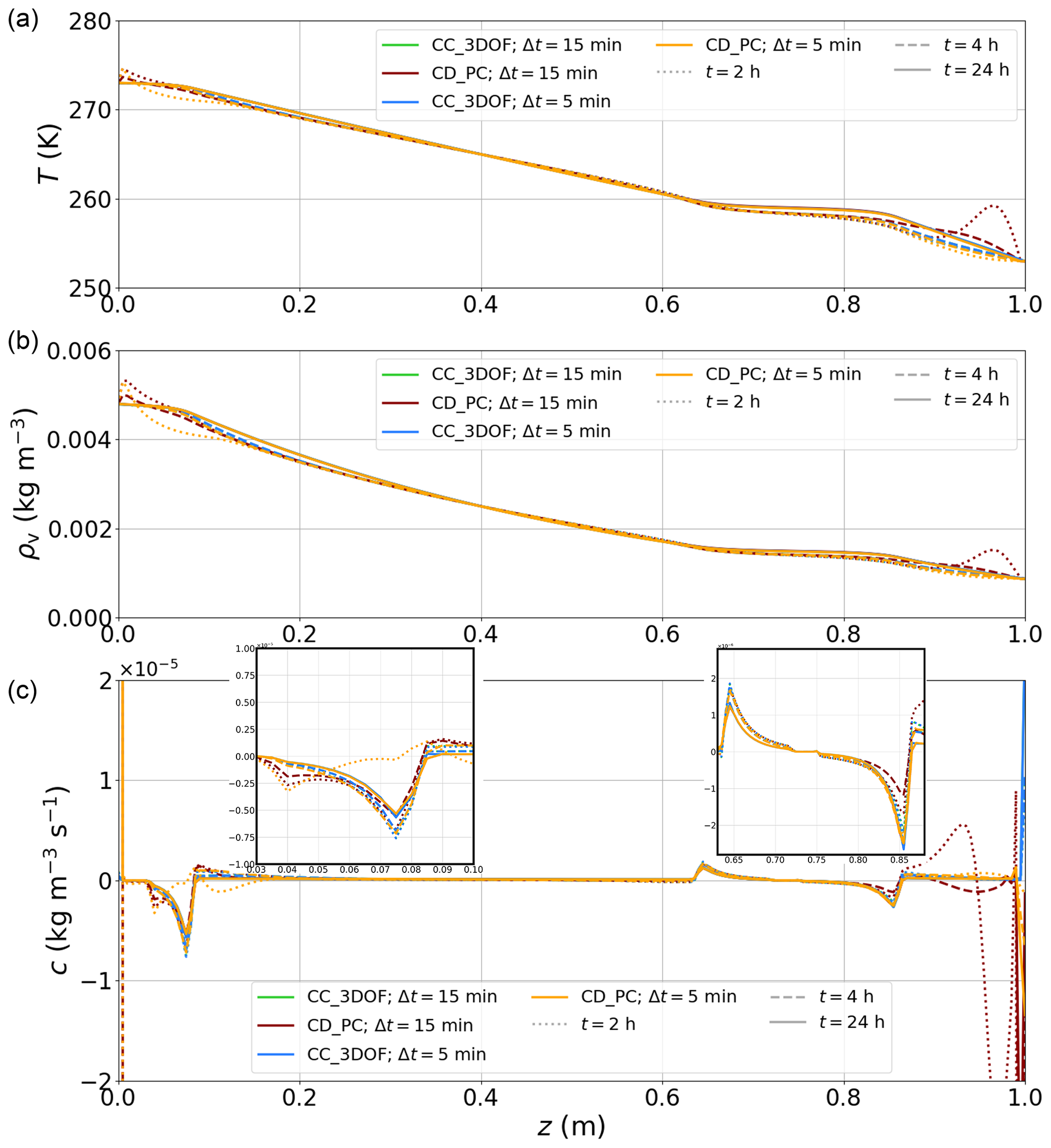
Figure 4 Comparison of temperature (a), water vapor density (b), and deposition rate (c) fields produced by CC_3DOF and CD_PC with Δt=5 min and Δt=15 min. Solutions are shown after 2, 4, and 24 h of simulation. A zoomed-in view of the deposition peaks is included in panel (c). Note that the green and blue lines are almost superimposed in all panels.

The much higher stability of CD_PC compared with CD_FD is due to the proper treatment of the reaction term in the water vapor mass balance equation, which acts as an attractor of ρ_v toward ${\mathit{\rho }}_{\mathrm{v}}^{\mathrm{eq}}$. Nevertheless, the results presented in this paragraph underline the major importance of having a coupled solution of the coupled heat and water vapor diffusion equations. Although the CD_PC approach gives steady solutions that are close to those obtained with the coupled approaches, the accuracy of the transient responses is essential, as the external forcings are constantly evolving in time for the vast majority of real-world configurations.

The same experiment has been run with the H_MF and H_TF configurations (not shown). The two strategies produce solution fields of T (and, consequently, of ρ_v and c, as both fields are diagnosed from the obtained T field) that are very close to each other and that show very little sensitivity to the time step size: the RMSD between both strategies after 24 h of simulation with Δt=5 min (Δt=15 min) is $\mathrm{6.2}\times {\mathrm{10}}^{-\mathrm{3}}$ K ($\mathrm{6.2}\times {\mathrm{10}}^{-\mathrm{3}}$ K), $\mathrm{5.6}\times {\mathrm{10}}^{-\mathrm{7}}$ kg m⁻³ ($\mathrm{5.5}\times {\mathrm{10}}^{-\mathrm{7}}$ kg m⁻³), and $\mathrm{7.3}\times {\mathrm{10}}^{-\mathrm{9}}$ $\mathrm{kg}{\mathrm{m}}^{-\mathrm{3}}{\mathrm{s}}^{-\mathrm{1}}$ ($\mathrm{7.3}\times {\mathrm{10}}^{-\mathrm{9}}$ $\mathrm{kg}{\mathrm{m}}^{-\mathrm{3}}{\mathrm{s}}^{-\mathrm{1}}$) for the T, ρ_v, and c fields, respectively. As we shall see in Sect. 4.4, only the H_MF approach shows perfect energy conservation.

4.3 Comparing the Hansen and Calonne systems for high α

Figure 5 shows the solutions produced after 38 h with our model using the following configurations: (1) H_MF and (2) CC_3DOF for various values of the sticking coefficient α. All simulations are run with the proper form of the mass matrices from the numerical setup introduced above, except for the BCs for ρ_v which are forced to no flux in all cases (Table 2) so that both configurations are easily comparable (see Sect. 4.6). For both configurations, effective parameters are computed from the Calonne parameterizations (Appendix A). We recall that the Calonne system has been derived via the two-scale expansion method that is valid for low reaction rates only, i.e., $\mathit{\alpha }\sim {\mathrm{10}}^{-\mathrm{3}}$ or less (Sect. 2.1). Therefore, neither the Calonne system nor the Calonne parameterization of effective parameters is expected to be valid for higher values of α. However, in a similar vein to Schürholt et al. (2022b), our goal here is simply to compare the mathematical behaviors of the Hansen and Calonne systems when they are run with the same parameterizations, independently of the physical soundness of obtained results.

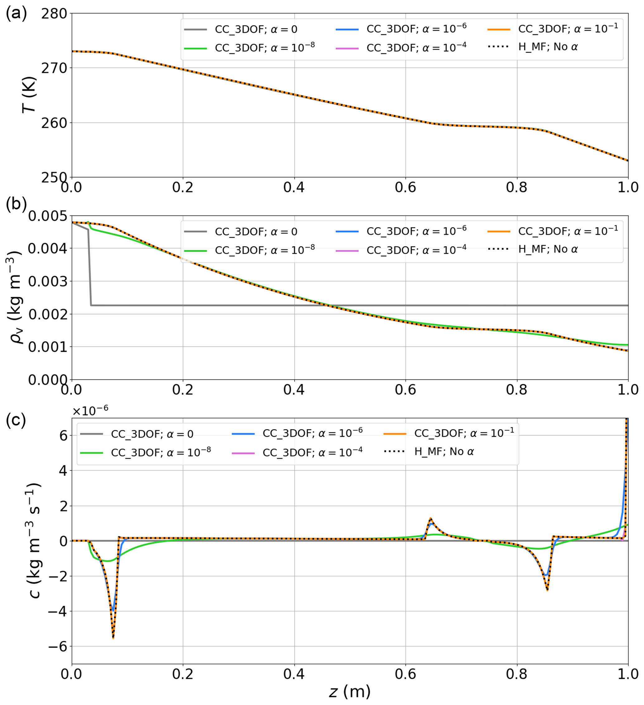
Figure 5 Comparison of temperature (a), water vapor density (b), and deposition rate (c) fields produced after 38 h of simulation with H_MF and with CC_3DOF for various values of α. Note that the case α=1 is not represented, as it would not be distinguishable from the case $\mathit{\alpha }={\mathrm{10}}^{-\mathrm{1}}$.

The solution fields produced by CC_3DOF progressively converge to those produced by H_MF as α increases and a higher reaction rate forces the vapor to saturation. This behavior was expected. Indeed, if effective parameters are calculated the same way and BCs are identical, both systems are formally equivalent when water vapor density is assumed to always be at saturation (Sect. 2.3). To quantify this behavior, Table 3 gathers all RMSDs between solutions produced at the end of the simulation by (1) H_MF and (2) CC_3DOF for all tested values of α.

Table 3 RMSDs between solutions obtained with H_MF and with CC_3DOF for the various values of α.

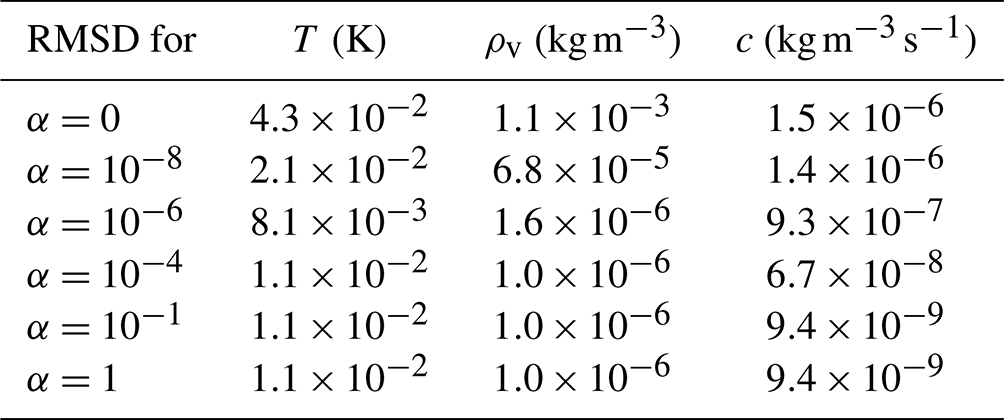
The difference in ρ_v and c between H_MF and CC_3DOF becomes less than 1 % when α becomes higher than 10⁻⁶ and 10⁻³, respectively. Below these values of α, the difference varies from a few percent to ∼100 % as α tends to 0. In contrast, T is less affected by the value of α. Even for the lowest values tested, the differences between the fields of T produced by H_MF and CC_3DOF are below 0.1 % (all lines are superimposed in Fig. 5a).

All together, these results seem to contradict those presented in Fig. 2 of Schürholt et al. (2022b): in their case, the solution fields (especially c) produced by the Hansen and Calonne models differ significantly, even when both models rely on the Calonne parameterizations for effective parameters. We think that this is due to the improper treatment of the mass matrices in their FEniCS implementation. This conclusion is supported by the fact that “existing continuum-mechanical models derived through homogenization (i.e., Calonne) or mixture theory (i.e., Hansen) yield similar results for homogeneous snowpacks of constant density” (Schürholt et al., 2022b), as demonstrated from their Scenario 1. Indeed, when density is uniform, the multiplying factors of the accumulation terms are independent of space and can be arbitrarily affected directly to the mass matrix or their inverses to the stiffness matrix and force vector.

4.4 On energy conservation

In order to evaluate how the different numerical strategies behave with respect to energy conservation, we run a slightly modified version of the numerical setup introduced in Sect. 4.1: the original Dirichlet BCs are replaced by no-flux BCs for both heat and vapor. Because settlement is deactivated (no vapor expelled from the snowpack to the atmosphere), the system is closed and all recorded energy leakage should be considered to be a numerical artifact. We run the experiment for 5 d, testing all strategies of the three options presented in Sect. 3.2 and summarized in Fig. 1b, except CD_FD which yields unrealistic results even for a time step as low as Δt=1 s. All experiments are run twice: once with Δt=15 min and another time with Δt=5 min. Then, the feedback of deposition on Φ_i is deactivated and the procedure is repeated. The obtained energy leakage is represented as a function of time in Fig. 6. Again, results produced with CC_3DOF are very close to those obtained with CC_2DOF, and only the former are reported. The total energy leakage at the end of the simulation is summarized in Table 4.

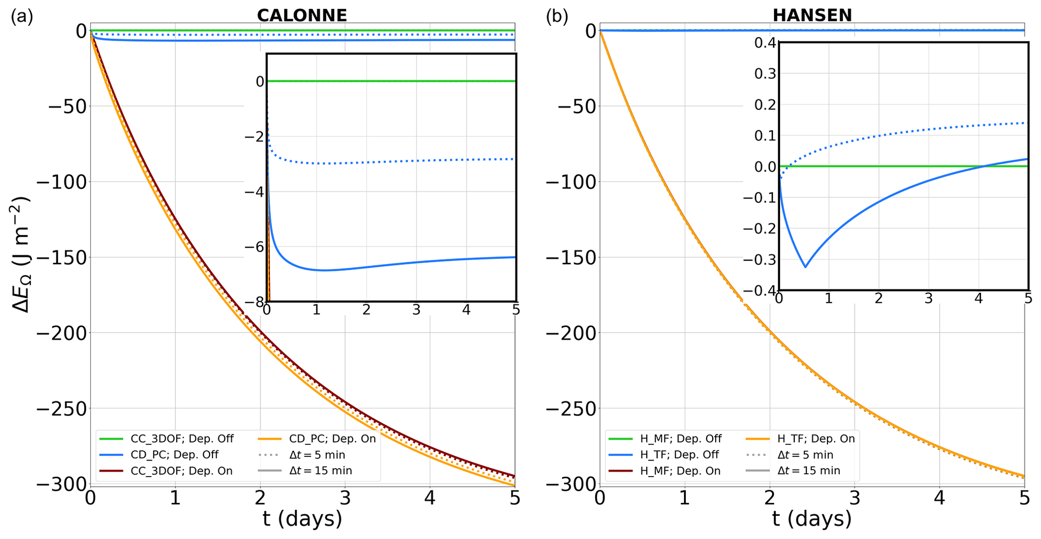
Figure 6 Energy leakage as a function of simulation time for the Calonne (a) and Hansen (b) systems, with and without deposition. For the Calonne system, we test the CC_3DOF and CD_PC strategies. For the Hansen system, we test the H_MF and H_TF strategies. Each simulation is run with Δt=5 min and Δt=15 min. Note that orange and red lines are almost superimposed in panel (b). Both panels contain a zoomed-in view of the region around ΔE_Ω=0 J m⁻².

Table 4 Total energy leakage (J m⁻²) after 5 d of simulation.

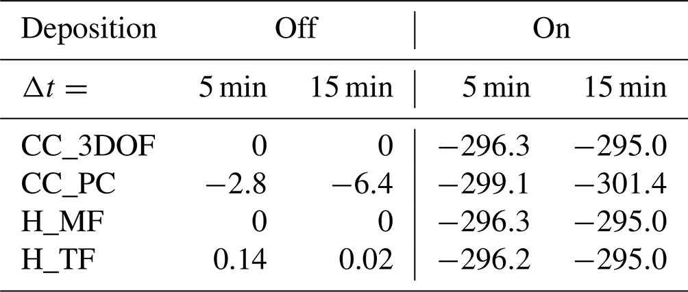
As expected, decoupling the deposition-related evolution of Φ_i (source term of the ice mass conservation equation) from the heat/vapor transfer equation induces an artificial energy loss of ∼300 J m⁻² for all considered cases at the end of the simulation. This energy loss remains very limited compared with the total energy contained in the system but could become noticeable for simulations on seasonal timescales and/or for configurations associated with stronger deposition rates. On the contrary, when deposition is omitted, energy leakage become negligible. Nevertheless, we stress that, contrary to the CC_2DOF, CC_3DOF, and H_MF strategies that are rigorously conservative, the CD_PC and H_TF strategies induce tiny but nonzero energy leakage, in line with the demonstration of Tubini et al. (2021). This illustrates that a rigorously energy-conservative solution of the problem of heat conduction and water vapor diffusion in snow implies solving the heat diffusion, water vapor diffusion, and ice mass conservation equations in a coupled way for the Calonne system and opting for the mixed form of the heat equation for the Hansen system.

4.5 On mass conservation

In this part, we reproduce the numerical setup corresponding to the Case 6 designed by Simson et al. (2021): we consider a snowpack with an initial thickness of 50 cm split into two equally thick snow layers of uniform initial densities, i.e., 150 kg m⁻³ for the lower one and 75 kg m⁻³ for the top one. All simulations are run considering only the settlement process. Our goal is to illustrate how the modifications made to the settlement scheme of Simson et al. (2021) affect the mass conservation and settlement rates. For this, we run the code of Simson and Kowalski (2021) with three bug fixes that are described in Appendix D. In particular, the strain rate governing the deformation of the whole space interval comprised between nodes k and k+1 is calculated from the stress and viscosity evaluated at node k (and not at node k+1 as in the published version of the code; Appendix D1). Simulations are run for 20 d, with Δt=15 min, and with three initially uniform meshes containing 11, 51, and 101 nodes, respectively. For all runs, viscosity is calculated from Eq. (A7) with a fixed temperature set to T=263 K.

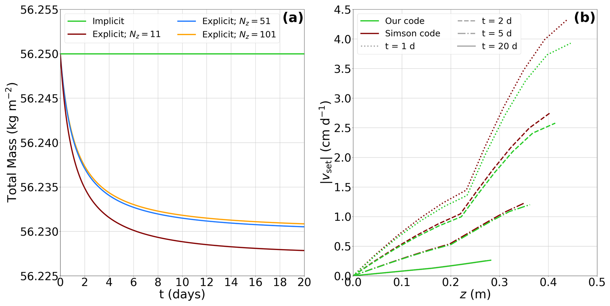
Figure 7 Panel (a) shows the evolution of the total mass over time when Φ_i is updated using the original explicit time discretization scheme implemented by Simson and Kowalski (2021) for meshes containing 11, 51, and 101 nodes. As soon as the time discretization scheme becomes implicit, mass is conserved independently of mesh refinement (green line). Panel (b) shows the absolute settling velocity profile obtained on the 11-node mesh with our model and with the corrected code of Simson et al. (2021) using an implicit time discretization scheme after 1, 2, 5, and 20 d of simulation.

We first run the simulations using the original explicit time discretization scheme implemented by Simson and Kowalski (2021) to update Φ_i. As illustrated in Fig. 7a, mass is not conserved in this case: there is an artificial mass loss that gets higher for coarser meshes. In the present case, this mass loss is in the order of 20 g after 20 d of simulation for a total initial mass of 56.25 kg. Although this mass loss tends to stabilize after a few days as viscosity increases exponentially with increasing Φ_i, it will become more significant when integrated over a full season characterized by regular snowfalls of low initial densities. As soon as the explicit time integration scheme is replaced by an implicit one, i.e., following Eq. (19) and Appendix D4, mass is perfectly conserved regardless of the mesh size. Note that this is the case when running both a corrected version of the code published by Simson and Kowalski (2021), in which the explicit settlement scheme has been replaced by an implicit one, and our model (green line in Fig. 7a). In Fig. 7b, we compare the settlement rates obtained with the code of Simson and Kowalski (2021) using the implicit time integration scheme to the one obtained with our code for an 11-node mesh. Using the approach of Simson and Kowalski (2021) corrected following Appendix D1 to ensure conservation of mass, the deformation of the whole numerical layer between k and k+1 is implicitly calculated from the stress evaluated at the bottom node of the layer, where it is maximal. In contrast, we assess the deformation occurring between nodes k and k+1 by integrating the ratio between the stress and viscosity fields along the element $k+\mathrm{1}/\mathrm{2}$. As a consequence, the former treatment tends to slightly overestimate the settlement rate compared with ours. This sensitivity is stronger at the beginning of the simulation when settlement rates are higher, and it tends to decrease over time. As expected, when the mesh resolution is increased, the two approaches converge to the same settlement rates (not shown).

4.6 On the boundary conditions for water vapor density

In this part, we want to highlight the sensitivity of the solution fields to the treatment of water vapor at boundaries. To this end, we reproduce Case 7 proposed by Simson et al. (2021). Case 7 corresponds to the same numerical setup as that of Case 6 introduced above, but the heat and water vapor diffusion processes are included. Furthermore, the feedback of temperature on viscosity is taken into account via Eq. (A7).

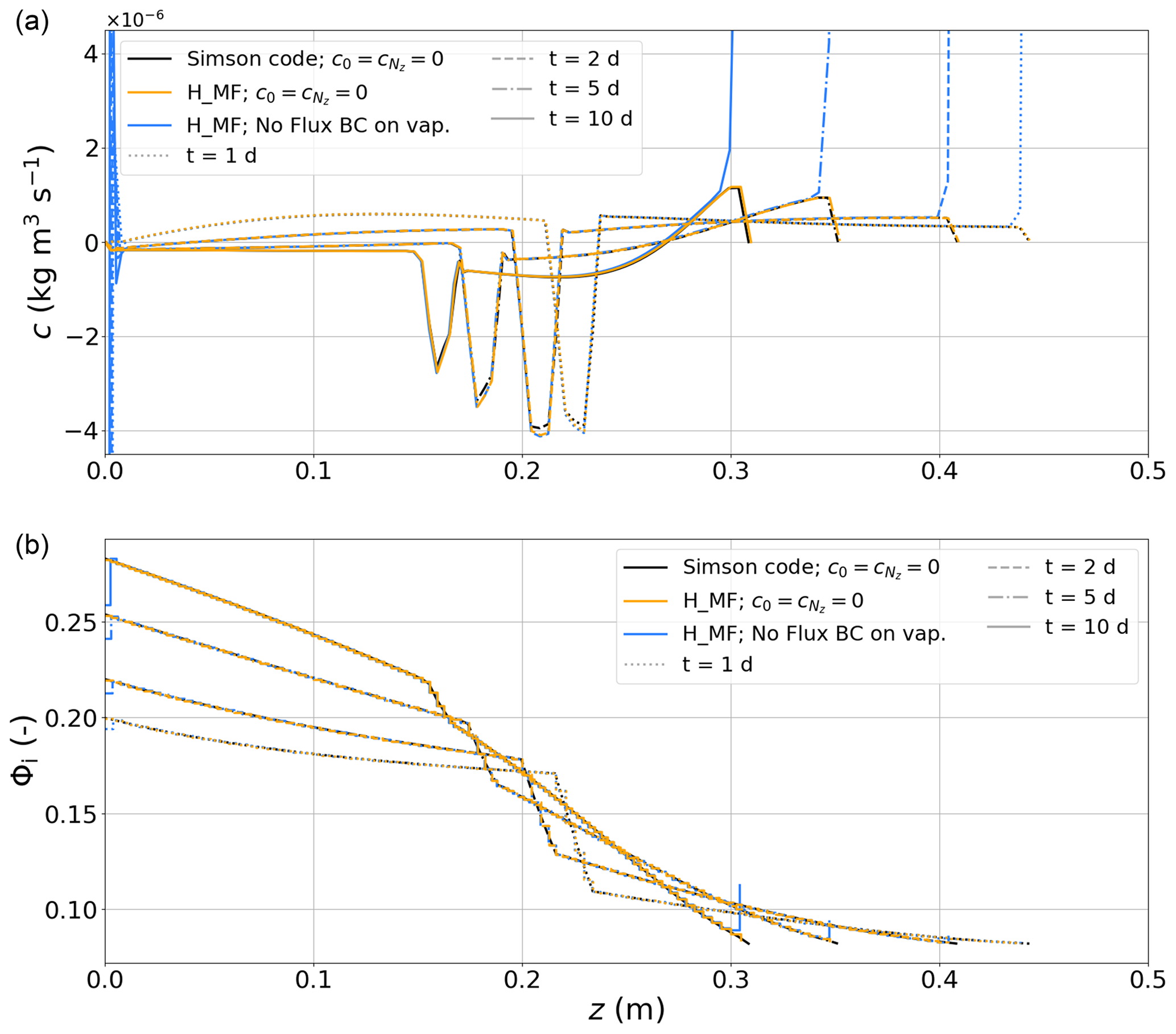
Figure 8 Comparison of deposition rate (a) and ice volume fraction (b) fields produced after 1, 2, 5, and 10 d of simulation on a 101-node mesh running (i) the corrected version of the code published by Simson et al. (2021), (ii) H_MF with boundary values of c forced to zero, and (iii) H_MF with no constraint on boundary values of c but with a no-flux BC on vapor. Note that, as it is an element-wise variable in our approach, Φ_i is represented as steps for the two H_MF cases.

Figure 8 shows the c and Φ_i fields obtained after 1, 2, 5, and 10 d of simulation on a 101-node mesh when running the code published by Simson and Kowalski (2021) with an implicit settlement scheme and with the bug fixes described in Appendix D (black lines in Fig. 8a). The values of c are always zero at the boundaries because they are forced as such in the model by the authors. Despite slight differences in the numerical implementation (e.g., element-wise vs. nodal nature of Φ_i, treatment of the strain rate, and mixed form vs. T form for the Hansen system), running our model in its H_MF configuration gives solution fields that are consistent with those produced by the code of Simson and Kowalski (2021) if we also force the boundary values of c to zero (orange lines in Fig. 8a). Concretely, the RMSDs for c vary between $\mathrm{2.8}\times {\mathrm{10}}^{-\mathrm{8}}$ and $\mathrm{3.4}\times {\mathrm{10}}^{-\mathrm{8}}$ $\mathrm{kg}{\mathrm{m}}^{-\mathrm{3}}{\mathrm{s}}^{-\mathrm{1}}$, corresponding to differences in the order of ∼1 %.

As stated in Sect. 3.2, because the deposition rate is derived as the closure of the water vapor mass balance, imposing a vanishing deposition rate at a boundary is equivalent to imposing a boundary vapor flux that adjusts itself so that local disequilibrium between ρ_v and ${\mathit{\rho }}_{\mathrm{v}}^{\mathrm{eq}}$ are entirely compensated for without any requirements for phase change. This choice is arbitrary and cannot be used as the generic BC for snowpack models. Ideally, the BCs for the vapor mass budget should be derived through a vapor budget at interfaces (akin to the surface energy budget routinely used as BCs for the energy equation). The importance of the BCs for vapor can be illustrated by running the same H_MF simulation as above but removing all constraints on c and assuming no vapor fluxes at boundaries. The resulting field of c is then characterized by peak values at the two boundary nodes, which depart significantly from the distribution of c in the interior of the domain (blue lines in Fig. 8a). These high deposition rates at domain boundaries have direct implications for the field of Φ_i: a significant part of the ice mass of the bottom element sublimates and is transported upwards. This leads to a situation in which the bottom element is less dense than the one immediately above, a tendency that is exacerbated over time (blue lines in Fig. 8b). This behavior creates strong local density gradients that seem to trigger self-amplifying oscillations at the bottom boundary: a sublimation peak at the bottom node is followed by a deposition peak at the node right above. This oscillatory pattern propagates inwards over a number of nodes that grows in time. On the top, strong mass gain occurs associated with a high deposition peak over the top element but does not trigger oscillations at this point in time. We stress that the peaks in c at boundaries and oscillations at the bottom boundary are not numerical artifacts but are truly part of the solution of Eq. (3) without vapor fluxes at the boundaries. They must be seen as the deposition rates that are required so that the Hansen system assumption regarding the permanent and instantaneous restoration of the water vapor density to its saturated value is fulfilled when no contribution can be expected from water vapor mass fluxes at the domain boundaries to bridge the gap.

4.7 On the formation of density wave instabilities

In their work, Schürholt et al. (2022b) used a dedicated numerical setup to illustrated that both the Hansen and Calonne systems are prone to producing self-amplifying spatial oscillations in the c and Φ_i fields when regions of very high density gradients are present, while linear stability analysis was utilized to confirm their results. These oscillations are true mathematical features related to the dependence of the effective heat and vapor diffusion coefficients on the ice volume fraction (Schürholt et al., 2022b). Here, we reproduce their experiment to investigate how this instability materializes when Φ_i is treated as an element-wise variable rather than a nodal variable. The numerical setup consists of a 2 cm thick snowpack with an initial ice volume fraction mimicking a Gaussian crust following Eq. (20) of Schürholt et al. (2022b) (solid black line in Fig. 9c). The initial conditions and BCs for T and ρ_v are the same as those used in Sect. 4.1. For these simulations, the time step is decreased to Δt=1 min.

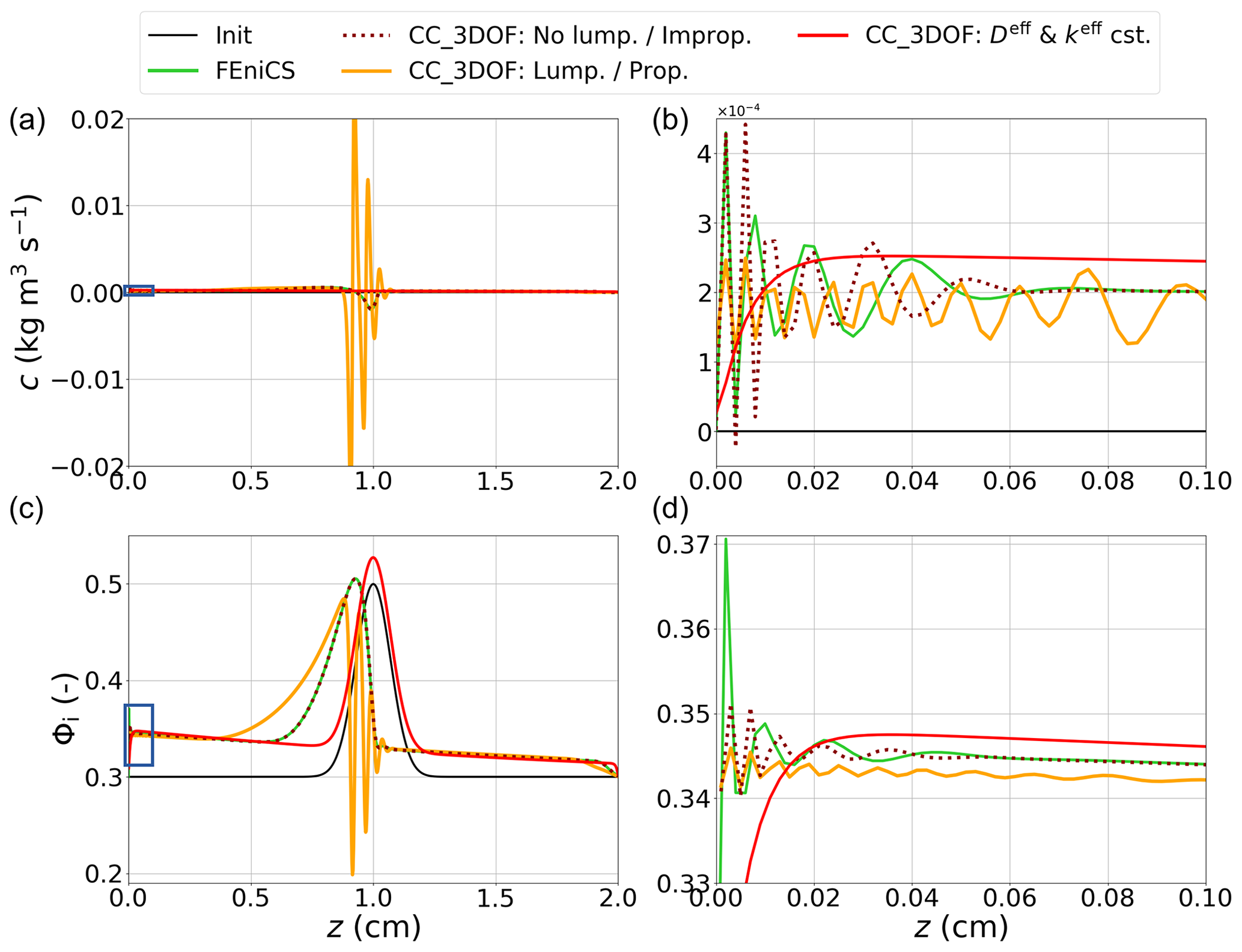
Figure 9 Comparison of deposition rate (a, b) and ice volume fraction (c, d) fields produced after 2 d of simulation on a 1000-node mesh by FEniCS, CC_3DOF without lumping and with the improper mass matrix, and CC_3DOF with lumping and with the proper mass matrix. The latter is run a second time with constant D^eff and k^eff. The blue boxes in panels (a) and (c) highlight the zoomed-in areas depicted in panels (b) and (d). The solid black lines correspond to the initial conditions. Note that, despite the element-wise nature of Φ_i in our model, the field of Φ_i is represented as lines drawn from elemental values affected to the middle of elements in order to ease comparison with the FEniCS solution.

Figure 9 shows the c and Φ_i fields obtained after 48 h of simulation on a 1000-node mesh. Let us compare first the solutions produced by FEniCS with an implicit time scheme (solid green line) and CC_3DOF with the same (improper) form of the mass matrix as for the FEniCS run and without lumping (dotted dark red line). Consistently with results already reported in Sect. 4.1, solutions obtained in both simulations are very close to each other. Concretely, RMSDs for c and Φ_i are $\mathrm{1.7}\times {\mathrm{10}}^{-\mathrm{5}}$ $\mathrm{kg}{\mathrm{m}}^{-\mathrm{3}}{\mathrm{s}}^{-\mathrm{1}}$ and $\mathrm{4.5}\times {\mathrm{10}}^{-\mathrm{4}}$, respectively. In addition, both approaches produce smooth wave patterns – for both c and Φ_i – encompassing several nodes at the bottom boundary. A closer look in this area (Fig. 9b, d) reveals slight differences. In particular, the amplitude of the oscillations in Φ_i are larger for the FEniCS solution than for the CC_3DOF one. This is not surprising given the nodal nature of Φ_i in the FEniCS approach: a deposition/sublimation peak at a given node translates directly into an ice volume fraction increase/decrease at the same node. In contrast, in our approach, the averaging of the nodal c over the elements when updating Φ_i (Sect. 3.3) tends to limit the amplitude of these oscillations, but it does not erase them. We also note that, contrary to the results reported in the previous section, no strong sublimation/deposition peaks are observed at the very bottom/top nodes. In fact, the deposition rate is very slightly positive at both nodes. This is because the Dirichlet BCs ${\mathit{\rho }}_{\mathrm{v}}={\mathit{\rho }}_{\mathrm{v}}^{\mathrm{eq}}$ applied to the water vapor mass balance equation of the Calonne system imply water vapor fluxes at boundaries that contribute to maintaining the saturation at these nodes, limiting the necessity for deposition/sublimation to bridge the oversaturation/undersaturation.

Running the same CC_3DOF simulation with the proper form of the mass matrix (solid orange line in Fig. 9) considerably changes the profiles of Φ_i and c obtained after 2 d of simulation. In particular, large oscillations in Φ_i related to large peaks in sublimation and deposition are observed on the sublimating (cold) side of the Gaussian crust. In fact, the general pattern of formation and propagation of the instability wave is not changed compared to the two previous simulations (as illustrated in Fig. 5 of Schürholt et al., 2022b), but oscillations set up at a much faster pace in this simulation. Again, this shows that treating mass matrices in their improper form can dramatically affect the obtained solutions at a given point in time.

We run an additional simulation that again consists of the CC_3DOF strategy with the proper form of the mass matrix and lumping activated but instead uses constant values for the effective parameters k^eff and D^eff. More specifically, we set k^eff=0.2 $\mathrm{W}{\mathrm{m}}^{-\mathrm{1}}{\mathrm{K}}^{-\mathrm{1}}$ and $D^{\mathrm{eff}}=\mathrm{1.066}\times {\mathrm{10}}^{-\mathrm{5}}$ m² s⁻¹. This corresponds to the Calonne parameterization of these effective parameters for a Φ_i fixed to its initial averaged value, i.e., Φ_i=0.318. The obtained solution shows a nonuniform deposition over the whole domain (solid red line in Fig. 9a and c). This is because the water vapor fluxes at boundaries implied by the previously mentioned Dirichlet BCs for water vapor bring enough water vapor mass from the exterior so that the whole layer is oversaturated for the implemented values of k^eff and D^eff, which causes deposition. In contrast, when the same simulation is run with a no-flux condition on vapor at boundaries, we observe a very strong peak in sublimation at the bottom node and a less pronounced peak in deposition at the top node (not shown). The nonuniform deposition leads to an increase in Φ_i over the whole domain (more pronounced on the lower half than on the upper half). Logically, the quasi-advection of the Gaussian crust towards the warm boundary that is observed in all other simulations and thoroughly analyzed by Schürholt et al. (2022b) does not occur here. Indeed, the aforementioned quasi-advection of the Gaussian crust towards the warm boundary is due to continuous deposition on the lower side of the crust associated with continuous sublimation on the upper side, which does not happen in this case. Another remarkable feature is the absence of the wave instability pattern in this case, in line with the prediction of Schürholt et al. (2022b).

All together, these observations confirm the assertion of Schürholt et al. (2022b): the wave patterns on c and Φ_i are intrinsic features of the mathematical models rather than due to, for example, the form of the implemented mass matrix or a violation of the DMP; they are triggered by strong density gradients and are due to the dependence of k^eff and D^eff on the ice volume fraction. There are slightly smoothened, but not removed, when the Φ_i is treated as an element-wise quantity rather than as a nodal quantity.

Note that we have also run the same experiment with the H_MF model using the Hansen parameterization of effective parameters (not shown). Again, our results are in line with those of Schürholt et al. (2022b): the wave instability appears much faster and with a much stronger amplitude than for the Calonne model with the Calonne parameterization of effective parameters.

4.8 On the effect of settlement on the density wave instabilities

We take advantage of our developments to run the same experiment as above but with settlement activated. As the considered domain is only 2 cm thick and the initial mean density is 291 kg m⁻³, the stresses are too low and the initial viscosity is too high (viscosity increases exponentially with density) to induce significant settlement in affordable computational time if the parameterization (Eq. A7) of viscosity is taken as such. Therefore, we decide to keep this parameterization but to divide the obtained viscosity by a factor 10⁴. Given the linear nature of the implemented constitutive law, the general pattern of deformation is expected to be kept but with a strongly enhanced settlement rate. We limit the simulations to two runs, both performed with the CC_3DOF strategy with the proper form of the mass matrix and with lumping activated: one is run with settlement on, whereas the other is run with settlement off.

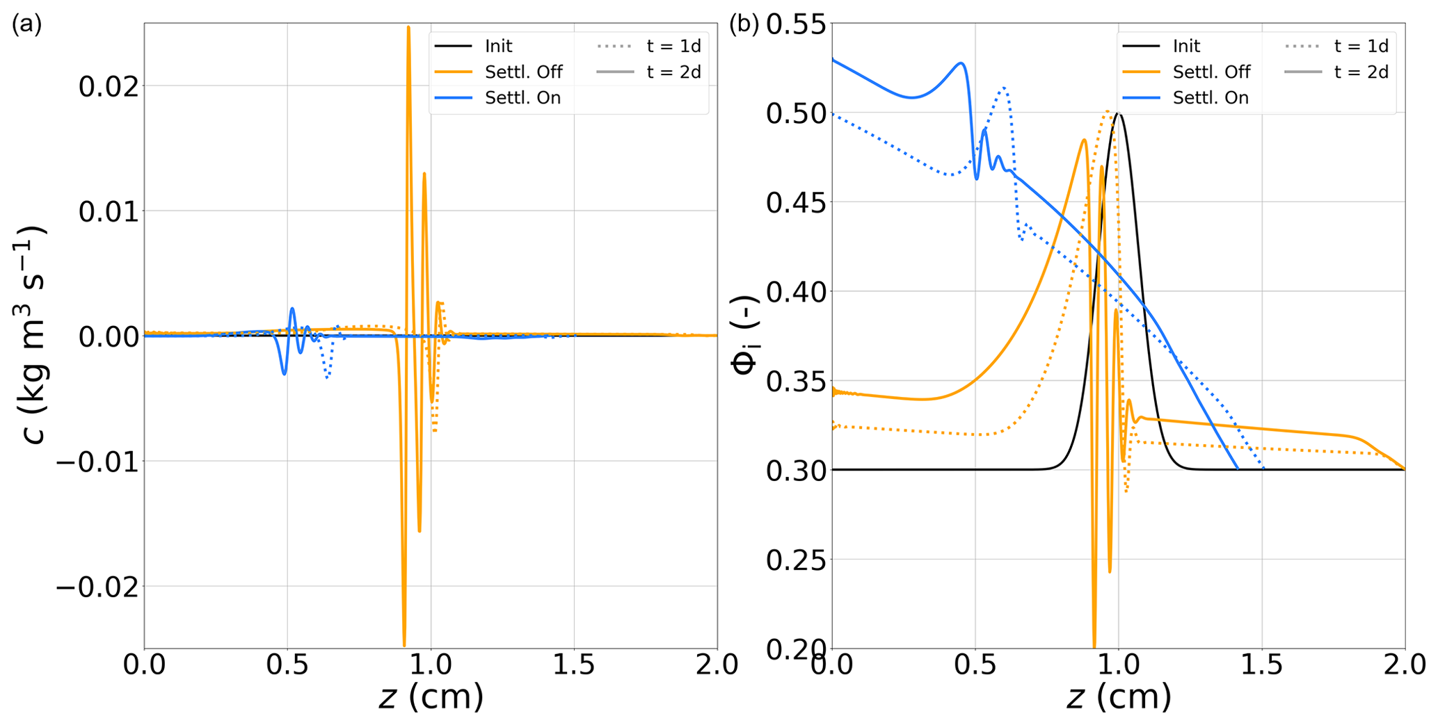
Figure 10 Comparison of deposition rate (a) and ice volume fraction (b) fields produced after 1 and 2 d of simulation on a 1000-node mesh by CC_3DOF with lumping and the proper mass matrix in two configurations: without and with settlement. The solid black lines correspond to the initial conditions. We opt for the same representation of Φ_i as in Fig. 9.

As illustrated in Fig. 10, including settlement has a stabilizing effect on the wave instability: oscillations in c and Φ_i are still observed but with strongly reduced amplitudes. For the considered numerical setup, the ratio between the maximum amplitudes of the oscillations observed on c (Φ_i) when settlement is included and when it is omitted is ∼40 % (∼30 %) after 1 d and ∼20 % (∼25 %) after 2 d. These oscillations also take longer to set up when considering settlement: after 1 d of simulation, they are only starting to affect the c field at the bottom nodes, and their feedback on the Φ_i field in this area is hardly perceptible. In contrast, when settlement is not included, the oscillatory pattern at the bottom boundary is already well established on both fields after 1 d of simulation. This stabilizing effect could be expected from the Φ_i dependence of viscosity: the denser the element, the less it deforms, and vice versa. This tends to homogenize the density of the snowpack and competes with phase change which, as shown previously, tends to further densify the denser layers and to further deplete the hollower layers. Another interesting feature is that, while only deposition is observed far enough from the Gaussian crust when settlement is off, these areas show sublimation when settlement is included.

5 Implications for future developments

The numerical issues that have been highlighted in the present work are relevant beyond the particular processes investigated here. First of all, it is a very general rule that the discretization of a continuous PDE must preserve its properties. First, this supposes the inclusion of any factor affecting the accumulation term in the corresponding mass matrix, but not its inverse in the stiffness matrix, as soon as such factor is nonuniform. Second, this contraindicates the use of the chain rule on the accumulation term during time discretization, as it might break the conservative properties of the continuous PDE. In fact, in many situations, it is preferable to treat such a PDE in its mixed form, i.e., with the time derivative of the accumulation term directly applied to the conserved quantity. This is a generic result for conservation equations and has already been illustrated for several other processes (e.g., Celia et al., 1990; Casulli and Zanolli, 2010; Tubini et al., 2021). We have also shown that two-way-coupled PDEs need to be solved as single monolithic process to preserve their conservative properties. In addition, depending on the relative dynamics of the subprocesses at stake, solving the latter sequentially might require one to considerably decrease the time step in order to guarantee acceptable transient solutions. A monolithic treatment of coupled equations does not fundamentally increase the complexity and numerical cost of the solution. Indeed, solving two decoupled tridiagonal systems of equations or solving one coupled pentadiagonal system of equations both come with the same complexity (i.e., 𝒪(n); El-Mikkawy and Atlan, 2014; Jia and Jiang, 2015). The possibility of using larger time steps with a monolithic treatment is, thus, beneficial in terms of computational cost. Again, this result holds as soon as two-way-coupled PDEs are at stake, in snow modeling or elsewhere.

More generally, coming up with a numerical implementation that guarantees energy and mass conservation is not straightforward. Therefore, a rigorous assessment of the evolution of energy and mass within the domain is a golden rule that should guide any numerical developments. This requires knowing the energy and mass fluxes in and out of the domain and, thus, explicitly computing the residuals of the algebraic system. In the eventuality that constraint on numerical cost requires numerical implementations violating the energy/mass conservation, the associated leakage should remain negligible, be well identified, and be tracked carefully. This is what we have done for the energy leakage associated with the sequential treatment of the feedback of deposition/sublimation on the ice mass conservation. Not only is this required to ensure that the model produces physically sound results but it is also required from the perspective of latter couplings to other components of Earth system models (ESMs). Indeed, the introduction of an artificial sink/source of energy/mass within ESMs obviously contributes to undesired model drift (e.g., Gupta et al., 2013; Hobbs et al., 2016). A good identification and a correct quantification of the spurious energy/mass leakage makes it easier to correct this drift.

More specific to the problem of water vapor diffusion is the treatment of water vapor at boundaries. We have shown (in Sect. 4.6) how sensitive the solution fields can be to this treatment. Previous works modeling macroscopic water vapor diffusion in snow have only considered two types of BCs for vapor: a no-flux condition (e.g., Touzeau et al., 2018) and a Dirichlet-type BC enforcing saturation of vapor at boundaries (e.g., Schürholt et al., 2022b). Jafari et al. (2020) used a mix of both, i.e., no flux at the bottom BC and saturation at the top BC. We also recall that forcing the deposition rate to zero at boundary nodes when solving the Hansen system, as done by Simson et al. (2021), is a roundabout way of arbitrarily prescribing vapor fluxes at boundaries that perfectly compensate for the oversaturation/undersaturation at these nodes. In natural configurations, vapor fluxes are expected at both boundaries. It follows that the proper way of proceeding for real-world applications is to solve a surface water vapor mass balance in order to derive well-defined boundary water vapor fluxes, similarly to what is normally done for energy. In contrast, cold-laboratory experiments can impose a no-flux condition on vapor at boundaries by using impermeable plates. Such experiments reveal strong sublimation at the bottom BC and strong deposition at the top BC (e.g., supplement of Hagenmuller et al., 2019; Bouvet et al., 2023). These observations are consistent with the peaks in sublimation/deposition obtained at the bottom/top boundaries when vapor is forced to no flux, as presented in Sect. 4.6.

These peaks in sublimation/deposition and the related local increase in density gradients are a trigger for wave instability. This behavior is carefully analyzed in the study of Schürholt et al. (2022b), who also discuss the implications for the numerical solution. The existence of such wave instability was already proposed by Adams and Brown (1990) from theoretical arguments. It is due to the dependence of the effective thermal conductivity and vapor diffusion coefficient on the ice volume fraction. Physically, we understand the mechanism as follows: water vapor diffuses less readily across regions with a higher ice volume fraction; because the thermal conductivity of air is about 100 times less than that of ice, temperature gradients are stronger in regions with a low ice volume fraction, and vapor fluxes are enhanced; these two phenomena combine to induce local accumulation of water vapor in places where the water vapor encounters an abrupt increase in the ice volume fraction in its flow towards decreasing temperatures; and this local accumulation leads to local oversaturation that is resorbed through deposition, further increasing the ice volume fraction at the transition. Similarly, when water vapor flows across an abrupt decrease in the ice volume fraction, enhanced water fluxes in the downstream low-density region combined with the difficulty in the upstream high-density region with respect to supplying water vapor lead to local undersaturation, which causes sublimation. Our developments have highlighted two stabilizing effects: one that is physical, i.e., the inclusion of settlement, and one that is numerical, i.e., the element-wise treatment of Φ_i. Given these two effects, and acknowledging the fact that the numerical setup considered here is rather extreme (macroscopic temperature gradient of 1000 K m⁻¹ and 1000 elements for a 2 cm thick snowpack), we think that this instability wave is unlikely to become a major modeling difficulty for many of the natural settings. This point is more hazardous for situations such as seasonal-scale simulations of thin arctic snowpacks, and more simulations covering a large range of realistic configurations are needed.

As discussed by Simson et al. (2021), the surface ice mass balance related to new precipitation or to sublimation (for dry snow) also has to be addressed. We think that our choice regarding the element-wise treatment of conserved quantities will greatly facilitate this implementation. For simulations on a seasonal timescale, occasional re-meshing will be necessary to limit the computational cost. Again, the element-wise nature of conserved quantities will enable unequivocal redistribution of the conserved quantities over merged or split elements. More generally, we draw the reader's attention to the widespread confusion between physical and numerical layers. Even when one claims to be adopting a continuous representation of the snowpack, the numerical solution of PDEs always requires discretization of the domain, which amounts to the definition of numerical layers. As soon as some integration is at stake (e.g., assessment of snowpack deformation from stress and viscosity), some assumption must necessarily be made about the evolution of fields within the numerical layers. Therefore, it is obviously preferable to have finer mesh in areas where gradients of relevant physical quantities are strong and a coarser mesh elsewhere. This is equivalent to saying that there must be some kind of correspondence between numerical and physical layers, if we define the latter as sections of the domain characterized by low gradients of physical properties.

The present work is a further step towards the development of the next generation of detailed snowpack models, associating sound and universal physics with a robust numerical treatment. So far, the implemented processes are limited to the coupled heat conduction, water vapor diffusion, and settlement in dry snow, but the numerical subtleties that have been highlighted are relevant for many other processes, in snow modeling and beyond. Our model is now ready to reproduce well-controlled laboratory experiments, provided that BCs are well constrained. In contrast, modeling natural settings will require more work, in particular regarding the energy, water vapor mass, and ice mass balances at boundaries. For longer-term developments, it will be necessary to implement other processes, notably those related to the liquid phase of water (melting/refreezing and percolation) as well as those regarding snow metamorphism.

Appendix A: Parameterizations used in our model

A1 Effective vapor diffusion coefficient

All simulations presented in the paper are run using the parameterization of the effective vapor diffusion coefficient proposed by Simson et al. (2021). It is based on the parameterization derived by Calonne et al. (2014), but it uses the Heaviside function Θ to hinder vapor diffusion for ice volumes above two-thirds. It is expressed as follows:

$$\begin{array}{}\text{(A1)}& D^{\mathrm{eff}}=D_{\mathrm{0}}\left(\mathrm{1}-{\displaystyle \frac{\mathrm{3}}{\mathrm{2}}}{\mathrm{\Phi }}_{\mathrm{i}}\right)\mathrm{\Theta }\left({\displaystyle \frac{\mathrm{2}}{\mathrm{3}}}-{\mathrm{\Phi }}_{\mathrm{i}}\right),\end{array}$$

with D₀ given in Table 1. Additional simulations mentioned in the paper were run using the parameterization of Hansen and Foslien (2015), which is expressed as follows:

$$\begin{array}{}\text{(A2)}& \begin{array}{rl}{D}^{\mathrm{eff}}& ={\mathrm{\Phi }}_{\mathrm{i}}(\mathrm{1}-{\mathrm{\Phi }}_{\mathrm{i}})D_{\mathrm{0}}\\ & +(\mathrm{1}-{\mathrm{\Phi }}_{\mathrm{i}})\left({\displaystyle \frac{k_{\mathrm{i}}{D}_{\mathrm{0}}}{{\mathrm{\Phi }}_{\mathrm{i}}\left(k_{\mathrm{a}}+L_{\mathrm{m}}{D}_{\mathrm{0}}\frac{\mathrm{d}{\mathit{\rho }}_{\mathrm{v},\mathrm{sat}}}{\mathrm{d}T}+(\mathrm{1}-{\mathrm{\Phi }}_{\mathrm{i}})k_{\mathrm{i}}\right)}}\right),\end{array}\end{array}$$

with all constant values listed in Table 1.

A2 Effective thermal conductivity

All simulations presented in the paper are run using the parameterization of Calonne et al. (2011) for the effective thermal conductivity, which is expressed as follows:

$$\begin{array}{}\text{(A3)}& k^{\mathrm{eff}}=k_{\mathrm{0}}+k_{\mathrm{1}}{\mathit{\rho }}_{\mathrm{i}}{\mathrm{\Phi }}_{\mathrm{i}}+k_{\mathrm{2}}({\mathit{\rho }}_{\mathrm{i}}{\mathrm{\Phi }}_{\mathrm{i}}{)}^{\mathrm{2}},\end{array}$$

where k₀=0.024 $\mathrm{W}{\mathrm{m}}^{-\mathrm{1}}{\mathrm{K}}^{-\mathrm{1}}$, $k_{\mathrm{1}}=-\mathrm{1.23}\times {\mathrm{10}}^{-\mathrm{4}}$ $\mathrm{W}{\mathrm{m}}^{\mathrm{2}}{\mathrm{K}}^{-\mathrm{1}}{\mathrm{kg}}^{-\mathrm{1}}$, and $k_{\mathrm{2}}=\mathrm{2.5}\times {\mathrm{10}}^{\mathrm{6}}$ $\mathrm{W}{\mathrm{m}}^{\mathrm{5}}{\mathrm{K}}^{-\mathrm{1}}{\mathrm{kg}}^{-\mathrm{2}}$. Additional simulations mentioned in the paper were run using the parameterization of Hansen and Foslien (2015), which is expressed as follows:

$$\begin{array}{}\text{(A4)}& \begin{array}{rl}{k}^{\mathrm{eff}}& ={\mathrm{\Phi }}_{\mathrm{i}}\left((\mathrm{1}-{\mathrm{\Phi }}_{\mathrm{i}})k_{\mathrm{a}}+{\mathrm{\Phi }}_{\mathrm{i}}{k}_{\mathrm{i}}\right)\\ & +(\mathrm{1}-{\mathrm{\Phi }}_{\mathrm{i}})\left({\displaystyle \frac{k_{\mathrm{i}}{k}_{\mathrm{a}}}{{\mathrm{\Phi }}_{\mathrm{i}}\left(k_{\mathrm{a}}+L_{\mathrm{m}}{D}_{\mathrm{0}}\frac{\mathrm{d}{\mathit{\rho }}_{\mathrm{v},\mathrm{sat}}}{\mathrm{d}T}+(\mathrm{1}-{\mathrm{\Phi }}_{\mathrm{i}})k_{\mathrm{i}}\right)}}\right),\end{array}\end{array}$$

with all constant values listed in Table 1.

A3 Effective heat capacity

Contrary to Simson et al. (2021) and Schürholt et al. (2022b), our parameterization of the effective heat capacity neglects the heat carried by dry air, which is then expressed as follows:

$$\begin{array}{}\text{(A5)}& {\left(\mathit{\rho }{C}_{\mathrm{p}}\right)}^{\mathrm{eff}}={\mathit{\rho }}_{\mathrm{i}}{C}_{\mathrm{i}}{\mathrm{\Phi }}_{\mathrm{i}},\end{array}$$

with all constant values given in Table 1. This assumption is justified by the small volumetric heat capacity of dry air compared with that of ice. This choice enables one to close the energy budget without having to track the dry air leaving the snowpack as it settles.

A4 Saturation water vapor density

All simulations presented in this paper are run using the parameterization of Libbrecht (1999) for the saturation water vapor density:

$$\begin{array}{}\text{(A6)}& {\mathit{\rho }}_{\mathrm{v}}^{\mathrm{eq}}={\displaystyle \frac{\exp (-T_{\mathrm{r}}/T)}{fT}}\left(a_{\mathrm{0}}+a_{\mathrm{1}}(T-T_{\mathrm{m}})+a_{\mathrm{2}}(T-T_{\mathrm{m}}{)}^{\mathrm{2}}\right),\end{array}$$

where T_r=6150 K, f=461.31 $\mathrm{J}{\mathrm{K}}^{-\mathrm{1}}{\mathrm{kg}}^{-\mathrm{1}}$, $a_{\mathrm{0}}=\mathrm{3.6636}\times {\mathrm{10}}^{\mathrm{12}}$ Pa, $a_{\mathrm{1}}=-\mathrm{1.3086}\times {\mathrm{10}}^{\mathrm{8}}$ Pa K⁻¹, $a_{\mathrm{2}}=-\mathrm{3.3793}\times {\mathrm{10}}^{\mathrm{6}}$ Pa K⁻², and T_m=273 K.

A5 Effective viscosity

All simulations presented in the paper are run using the viscosity parameterization of Vionnet et al. (2012):

$$\begin{array}{}\text{(A7)}& \mathit{\eta }({\mathrm{\Phi }}_{\mathrm{i}},T)=f{\mathit{\eta }}_{\mathrm{0}}{\displaystyle \frac{{\mathit{\rho }}_{\mathrm{i}}{\mathrm{\Phi }}_{\mathrm{i}}}{c_{\mathit{\eta }}}}\exp \left(a_{\mathit{\eta }}(T_{\mathrm{0}}-T)+b_{\mathit{\eta }}{\mathit{\rho }}_{\mathrm{i}}{\mathrm{\Phi }}_{\mathrm{i}}\right),\end{array}$$

with a fusion temperature of T₀=273 K; the constant parameters ${\mathit{\eta }}_{\mathrm{0}}=\mathrm{7.62237}\times {\mathrm{10}}^{\mathrm{6}}$ kg s⁻¹, a_η=0.1 K⁻¹, b_η=0.0.023 m³ kg⁻¹, and c_η=250 kg m⁻²; and an additional parameter f, which normally accounts for snow microstructure properties, that was set to f=1 in the present study.

Appendix B: Spatial and temporal discretization

The spatial discretization is based on the FEM. Indeed, the FEM enables a clear distinction between element-wise and nodal variables. The former are constant over elements and typically correspond to conserved quantities (e.g., ice volume fraction), whereas the latter are defined at mesh nodes, are continuous in space, and typically correspond to physical quantities driving the fluxes in between elements (e.g., temperature). As explained in further detail in Sect. 3.3, such a vision is consistent with the fact that the conservation of energy and mass are fulfilled on average per spatial interval rather than locally. In contrast to the work of Schürholt et al. (2022b), who used a Python-based FEM platform, we code every step of the method internally except the inversion of the linear system. This allows us to have complete control over the numerical implementation. Furthermore, this enables us to design a code structure that is well suited to snowpack modeling: each physical process corresponds to a module that can be easily activated or deactivated at the user's convenience. Below, we briefly recall the basics of the FEM. For more detail, we refer the reader to one of the many books that have been written on the subject (e.g., Pepper and Heinrich, 2005).

As the exact (analytical) solution u of a PDE is usually out of reach, the idea of the FEM is to find an approximate (numerical) solution $\stackrel{\mathrm{̃}}{u}$ in the following form:

$$\begin{array}{}\text{(B1)}& \stackrel{\mathrm{̃}}{u}(\mathbf{x},t)=\sum _{j=\mathrm{1}}^{N_{\mathrm{DOF}}}{\mathit{\phi }}_j\left(\mathbf{x}\right)u_j\left(t\right)\forall \mathbf{x}\in \mathrm{\Gamma },\end{array}$$

where Γ is the considered domain and the u_j represents the discrete unknown scalar values of the problem to be solved. The functions φ_j are linearly independent functions of space, referred to as the shape functions. Here, we follow the classical approach and adopt first-order Lagrangian polynomials as shape functions: the shape function φ_j is a continuous piecewise linear function, whose value equals 1 at the jth node and 0 at all other nodes. In this case, the unknown scalar value u_j simply corresponds to the value of $\stackrel{\mathrm{̃}}{u}$ at the jth node, and the shape functions φ_j can be viewed as linear interpolators in between nodes. The restriction of shape functions to first-order polynomials is motivated by the results of Schürholt et al. (2022b), who reported that, in their experiments, increasing the polynomial order was equivalent to increasing the mesh resolution with the corresponding number of nodes.

The PDE is then rewritten in its weak form, which consists of multiplying the PDE by any arbitrary test function and then integrating this product over Γ. Integration by parts is carried out on the divergence term to weaken the differentiation requirement of the solution field, which naturally makes boundary normal flux integrals arise. In order to obtain a closed set of discrete equations, the arbitrary test function is replaced by a finite set of test functions φ_i that are taken equal to the shape functions (standard Galerkin procedure). The problem is then reduced to solving N_DOF algebraic equations that can be cast into matrix forms, with matrix terms defined as integrals over space (see Appendix C). These integrals are evaluated using Gaussian quadratures. The Gaussian quadratures consist of replacing a continuous integral by a weighted sum of function values at specific points, the so-called Gaussian points, located within the elements. In particular, model parameters that depend on model variables are evaluated directly at Gaussian points at which nodal variables are interpolated through shape functions. When the considered model parameter is a nonlinear function of some model variable, this is different from evaluating the model parameter at nodes and then using shape functions to interpolate the obtained values at Gaussian point as done in studies such as Schürholt et al. (2022b). We use a default value of two Gaussian points per element, but this setting could easily be changed.

While the FEM provides a spatial discretization scheme, the obtained matrix equation also needs to be discretized in time. The θ method is the most commonly adopted. It consists of expressing all quantities as a weighted average between their values at the previous time step and their values at the current time step. In general, the matrix form of the resulting algebraic system is as follows:

$$\begin{array}{}\text{(B2)}& \begin{array}{rl}& \underset{\text{left-hand side matrix }\mathbf{A}}{\underbrace{\left[\mathbf{M}+\mathit{\theta }\mathrm{\Delta }t{\mathbf{K}}^{n+\mathrm{1}}\right]}}{\mathit{U}}^{n+\mathrm{1}}\\ & =\underset{\text{right-hand side vector }\mathit{B}}{\underbrace{\left[\mathbf{M}+(\mathit{\theta }-\mathrm{1})\mathrm{\Delta }t{\mathbf{K}}^n\right]{\mathit{U}}^n+\mathrm{\Delta }t\left[\mathit{\theta }{\mathit{F}}^{n+\mathrm{1}}+(\mathrm{1}-\mathit{\theta }){\mathit{F}}^n\right]}}\\ & +\mathrm{\Delta }t{\mathit{F}}^{\partial \mathrm{\Gamma }},\end{array}\end{array}$$

where the superscript n+1 (n) is applied to quantities evaluated at the current (previous) time step, Δt is the time step size, and U the solution vector. The matrices M and K are referred to as the mass and stiffness matrices, respectively. The vector F is called the force vector, and the vector F^∂Γ corresponds to boundary fluxes entering/leaving the domain during the time step. The particular cases of θ=0, θ=0.5, and θ=1 correspond to the first-order explicit Euler, the Crank–Nicolson, and the first-order implicit Euler methods, respectively. It can be shown that, whenever $\mathrm{0.5}\le \mathit{\theta }\le \mathrm{1}$, the time-stepping algorithm is L2 stable: the error between the continuous time derivative and its discrete counterpart remains bounded without any requirement with respect to the time step size. However, if the considered PDE is nonlinear, the system (Eq. B2) also becomes nonlinear for any θ>0. Such a system must be linearized. Linearization algorithms, such as the Picard or Newton techniques, are iterative methods that require the prescription of an initial guess, which must be sufficiently close to the solution to ensure convergence of the algorithm. The fulfillment of this condition hampers the prescription of an arbitrary large time step, even when the time discretization method is said to be unconditionally stable. On the other hand, while every case with θ≠0.5 is first order in time (i.e., the discretization error decreases linearly with Δt, as Δt converge to zero), the Crank–Nicolson method is second order in time (i.e., the discretization error decreases quadratically with Δt, as Δt converges to zero). This higher accuracy of the Crank–Nicolson method and its stability are often invoked to justify its use (e.g., Bader and Weilenmann, 1992; Decharme et al., 2011; Schürholt et al., 2022b). However, the obtained solution can be affected by spurious (decaying) oscillations if the time step is too large or the element size too small. For this reason, we prefer to use the standard first-order implicit Euler method (θ=1). Although potentially less accurate than the Crank–Nicolson method, the latter is more stable and less prone to oscillations (Formaggia and Scotti, 2011).

Specific BCs can be implemented via the appropriate modification of the matrix system (Eq. B2). More specifically, Neumann BCs can be directly implemented through the boundary flux vector F^∂Γ. A Dirichlet BC at a boundary node can be implemented by replacing its corresponding line in the left-hand-side matrix A of Eq. (B2) with the line of the identity matrix and setting the Dirichlet value in the right-hand-side vector B. Robin BCs must be seen as a weighted combination of Neumann and Dirichlet BCs in which the flux at the considered boundary is specified as a linear function of the value of the solution field at the corresponding boundary node. Implementing a Robin BC then consists of (i) adding the prescribed flux to the corresponding line of the boundary flux vector F^∂Γ and (ii) modifying the left-hand-side matrix A as for a Dirichlet BC, except that the diagonal term of the modified line, which is set to 1 when implementing a Dirichlet BC, must be set to the multiplying factor applying to the solution field in this case. The right-hand-side vector B is left unchanged.

Once the solution vector has been obtained, it is possible to diagnose the fluxes entering/leaving the system by calculating the matrix system residual, defined as $\mathrm{\Delta }t{\mathit{F}}^{\partial \mathrm{\Gamma }}=\mathbf{A}\mathit{U}-\mathit{B}$. Note that this operation applies for all types of BCs, notably Dirichlet conditions for which the boundary fluxes are not explicitly prescribed but, nonetheless, exist to maintain the boundary solution at its prescribed value. Assessing the boundary fluxes is necessary to verify the closure of the energy budget and can be required for latter coupling to external models.

Appendix C: Discrete forms of the systems of equations

This appendix presents the different FEM discretizations of the Calonne and Hansen systems for all considered strategies that are summarized in Fig. 1. In what follows, the functions φ_i and φ_j correspond to the test and shape functions, respectively.

C1 CC_3DOF

The Calonne system is solved for the solution vector $\mathit{u}=(T,{\mathit{\rho }}_{\mathrm{v}},c)$. The discrete system evaluated at nonlinear iteration k+1 can be expressed in matrix form as follows:

$$\begin{array}{}\text{(C1)}& \left\{\begin{array}{ll}{\mathbf{M}}_{\mathrm{T}}\dot{\mathit{T}}+{\mathbf{K}}_{\mathrm{T},\mathrm{T}}\mathit{T}+{\mathbf{K}}_{\mathrm{T},\mathrm{C}}\mathit{C}& ={\mathit{F}}_{\mathrm{T}}^{\partial \mathrm{\Gamma }}\\ {\mathbf{M}}_{\mathrm{P}}\dot{\mathit{P}}+{\mathbf{K}}_{\mathrm{P},\mathrm{P}}\mathit{P}+{\mathbf{K}}_{\mathrm{P},\mathrm{C}}\mathit{C}& ={\mathit{F}}_{\mathrm{P}}^{\partial \mathrm{\Gamma }}\\ {\stackrel{\mathrm{̃}}{\mathbf{M}}}_{\mathrm{C}}\mathit{C}+{\mathbf{K}}_{\mathrm{C},\mathrm{T}}\mathit{T}+{\mathbf{K}}_{\mathrm{C},\mathrm{P}}\mathit{P}& ={\mathit{F}}_{\mathrm{C}}.\end{array}\right.\end{array}$$

Here,

$$\begin{array}{}\text{(C2)}& {\displaystyle }{M}_{\mathrm{T}}^{i,j}=\underset{\mathrm{\Gamma }}{\int }{\left(\mathit{\rho }{C}_{\mathrm{p}}\right)}^{\mathrm{eff}}{\mathit{\phi }}_i{\mathit{\phi }}_j\mathrm{dV},\text{(C3)}& {\displaystyle }{M}_{\mathrm{P}}^{i,j}=\underset{\mathrm{\Gamma }}{\int }\left(\mathrm{1}-{\mathrm{\Phi }}_{\mathrm{i}}\right){\mathit{\phi }}_i{\mathit{\phi }}_j\mathrm{dV},\text{(C4)}& {\displaystyle }{\stackrel{\mathrm{̃}}{M}}_{\mathrm{C}}^{i,j}=\underset{\mathrm{\Gamma }}{\int }{\mathit{\phi }}_i{\mathit{\phi }}_j\mathrm{dV},\text{(C5)}& {\displaystyle }{K}_{\mathrm{T},\mathrm{T}}^{i,j}=\underset{\mathrm{\Gamma }}{\int }{k}^{\mathrm{eff}}\mathrm{\nabla }{\mathit{\phi }}_i\cdot \mathrm{\nabla }{\mathit{\phi }}_j\mathrm{dV},\text{(C6)}& {\displaystyle }{K}_{\mathrm{P},\mathrm{P}}^{i,j}=\underset{\mathrm{\Gamma }}{\int }{D}^{\mathrm{eff}}\mathrm{\nabla }{\mathit{\phi }}_i\cdot \mathrm{\nabla }{\mathit{\phi }}_j\mathrm{dV},\text{(C7)}& {\displaystyle }{K}_{\mathrm{T},\mathrm{C}}^{i,j}=\underset{\mathrm{\Gamma }}{\int }-L_{\mathrm{m}}{\mathit{\phi }}_i{\mathit{\phi }}_j\mathrm{dV},\text{(C8)}& {\displaystyle }{K}_{\mathrm{P},\mathrm{C}}^{i,j}=\underset{\mathrm{\Gamma }}{\int }{\mathit{\phi }}_i{\mathit{\phi }}_j\mathrm{dV},\text{(C9)}& {\displaystyle }{K}_{\mathrm{C},\mathrm{T}}^{i,j}=\underset{\mathrm{\Gamma }}{\int }s\mathit{\alpha }{v}_{\mathrm{kin}}\left(T^k\right){\left.{\displaystyle \frac{\mathrm{d}{\mathit{\rho }}_{\mathrm{v}}^{\mathrm{eq}}}{\mathrm{d}T}}\right|}_{T=T^k}{\mathit{\phi }}_i{\mathit{\phi }}_j\mathrm{dV},\text{(C10)}& {\displaystyle }{K}_{\mathrm{C},\mathrm{P}}^{i,j}=\underset{\mathrm{\Gamma }}{\int }-s\mathit{\alpha }{v}_{\mathrm{kin}}\left(T^k\right){\mathit{\phi }}_i{\mathit{\phi }}_j\mathrm{dV},\text{(C11)}& {\displaystyle }{F}_{\mathrm{C}}^i=\underset{\mathrm{\Gamma }}{\int }s\mathit{\alpha }{v}_{\mathrm{kin}}\left(T^k\right)\left({\left.{\displaystyle \frac{\mathrm{d}{\mathit{\rho }}_{\mathrm{v}}^{\mathrm{eq}}}{\mathrm{d}T}}\right|}_{T=T^k}{T}^k-{\mathit{\rho }}_{\mathrm{v}}^{\mathrm{eq}}\left(T^k\right)\right){\mathit{\phi }}_i\mathrm{dV}.\end{array}$$

In the above expressions, the saturation vapor density ${\mathit{\rho }}_{\mathrm{v}}^{\mathrm{eq}}$ has been linearized through Eq. (8), while v_kin is fixed from the temperature field T^k obtained at the previous nonlinear iteration. Vectors ${\mathit{F}}_{\mathrm{T}}^{\partial \mathrm{\Gamma }}$ and ${\mathit{F}}_{\mathrm{P}}^{\partial \mathrm{\Gamma }}$ correspond to normal boundary fluxes of sensible heat and vapor, respectively. Additional internal sources of energy besides the phase-change-related latent heat effect could easily be added as a force vector in the energy budget equation. Finally, note that the matrix ${\stackrel{\mathrm{̃}}{\mathbf{M}}}_{\mathrm{C}}$ is not a true mass matrix in the sense that it does not apply to a time derivative; therefore, it must be treated carefully during the time-stepping assembly (Eq. B2).

C2 CC_2DOF

The Calonne system is solved for the solution vector $\mathit{u}=(T,{\mathit{\rho }}_{\mathrm{v}})$. The discrete system evaluated at nonlinear iteration k+1 can be expressed in matrix form as follows:

$$\begin{array}{}\text{(C12)}& \left\{\begin{array}{ll}{\mathbf{M}}_{\mathrm{T}}\dot{\mathit{T}}+{\mathbf{K}}_{\mathrm{T},\mathrm{T}}\mathit{T}+{\mathbf{K}}_{\mathrm{T},\mathrm{P}}\mathit{P}& ={\mathit{F}}_{\mathrm{T}}+{\mathit{F}}_{\mathrm{T}}^{\partial \mathrm{\Gamma }}\\ {\mathbf{M}}_{\mathrm{P}}\dot{\mathit{P}}+{\mathbf{K}}_{\mathrm{P},\mathrm{P}}\mathit{P}+{\mathbf{K}}_{\mathrm{P},\mathrm{T}}\mathit{T}& ={\mathit{F}}_{\mathrm{P}}+{\mathit{F}}_{\mathrm{P}}^{\partial \mathrm{\Gamma }}.\end{array}\right.\end{array}$$

Here,

$$\begin{array}{}\text{(C13)}& {\displaystyle }\begin{array}{rl}& K_{\mathrm{T},\mathrm{T}}^{i,j}=\\ & \underset{\mathrm{\Gamma }}{\int }\left[k^{\mathrm{eff}}\mathrm{\nabla }{\mathit{\phi }}_i\cdot \mathrm{\nabla }{\mathit{\phi }}_j+L_{\mathrm{m}}s\mathit{\alpha }{v}_{\mathrm{kin}}\left(T^k\right){\left.{\displaystyle \frac{\mathrm{d}{\mathit{\rho }}_{\mathrm{v}}^{\mathrm{eq}}}{\mathrm{d}T}}\right|}_{T=T^k}{\mathit{\phi }}_i{\mathit{\phi }}_j\right]\mathrm{dV},\end{array}\text{(C14)}& {\displaystyle }{K}_{\mathrm{P},\mathrm{P}}^{i,j}=\underset{\mathrm{\Gamma }}{\int }\left[D^{\mathrm{eff}}\mathrm{\nabla }{\mathit{\phi }}_i\cdot \mathrm{\nabla }{\mathit{\phi }}_j+s\mathit{\alpha }{v}_{\mathrm{kin}}\left(T^k\right){\mathit{\phi }}_i{\mathit{\phi }}_j\right]\mathrm{dV},\text{(C15)}& {\displaystyle }{K}_{\mathrm{T},\mathrm{P}}^{i,j}=\underset{\mathrm{\Gamma }}{\int }-L_{\mathrm{m}}s\mathit{\alpha }{v}_{\mathrm{kin}}\left(T^k\right){\mathit{\phi }}_i{\mathit{\phi }}_j\mathrm{dV},\text{(C16)}& {\displaystyle }{K}_{\mathrm{P},\mathrm{T}}^{i,j}=\underset{\mathrm{\Gamma }}{\int }-s\mathit{\alpha }{v}_{\mathrm{kin}}\left(T^k\right){\left.{\displaystyle \frac{\mathrm{d}{\mathit{\rho }}_{\mathrm{v}}^{\mathrm{eq}}}{\mathrm{d}T}}\right|}_{T=T^k}{\mathit{\phi }}_i{\mathit{\phi }}_j\mathrm{dV},\text{(C17)}& {\displaystyle }{F}_{\mathrm{T}}^i=\underset{\mathrm{\Gamma }}{\int }{L}_{\mathrm{m}}s\mathit{\alpha }{v}_{\mathrm{kin}}\left(T^k\right)\left({\left.{\displaystyle \frac{\mathrm{d}{\mathit{\rho }}_{\mathrm{v}}^{\mathrm{eq}}}{\mathrm{d}T}}\right|}_{T=T^k}{T}^k-{\mathit{\rho }}_{\mathrm{v}}^{\mathrm{eq}}\left(T^k\right)\right){\mathit{\phi }}_i\mathrm{dV},\text{(C18)}& {\displaystyle }{F}_{\mathrm{P}}^i=\underset{\mathrm{\Gamma }}{\int }-s\mathit{\alpha }{v}_{\mathrm{kin}}\left(T^k\right)\left({\left.{\displaystyle \frac{\mathrm{d}{\mathit{\rho }}_{\mathrm{v}}^{\mathrm{eq}}}{\mathrm{d}T}}\right|}_{T=T^k}{T}^k-{\mathit{\rho }}_{\mathrm{v}}^{\mathrm{eq}}\left(T^k\right)\right){\mathit{\phi }}_i\mathrm{dV}.\end{array}$$

In the above expressions, M_T and M_P are expressed as in the CC_3DOF case. Again, additional internal sources of energy could easily be added in the force vector F_T if needed, and the nonlinearity due to ${\mathit{\rho }}_{\mathrm{v}}^{\mathrm{eq}}$ and v_kin is treated as for the CC_3DOF case. The field of c is then diagnosed in a next step as the closure of the water vapor mass balance equation, where ρ_v is set to the obtained solution field.

C3 CD_PC

The equations of the Calonne system are solved sequentially. In a first step, the heat equation is solved for T with a source term that is fixed from the c field computed at the previous time step. The discrete counterpart of this equation can be expressed in matrix form as follows:

$$\begin{array}{}\text{(C19)}& {\mathbf{M}}_{\mathrm{T}}\dot{\mathit{T}}+{\mathbf{K}}_{\mathrm{T},\mathrm{T}}\mathit{T}={\mathit{F}}_{\mathrm{T}}+{\mathit{F}}_{\mathrm{T}}^{\partial \mathrm{\Gamma }},\end{array}$$

where

$$\begin{array}{}\text{(C20)}& F_{\mathrm{T}}^i=\underset{\mathrm{\Gamma }}{\int }{L}_{\mathrm{m}}c{\mathit{\phi }}_i\mathrm{dV}.\end{array}$$

In the above expressions, M_T and K_T,T are expressed as in the CC_3DOF case, and there is the possibility of adding additional internal sources of energy in F_T. The obtained solution field is used to fix the distributions of v_kin and ${\mathit{\rho }}_{\mathrm{v}}^{\mathrm{eq}}$. The water vapor mass balance equation can then be solved for ρ_v under its diffusion-reaction form in a second step. The discrete counterpart of this equation can be expressed in matrix form as follows:

$$\begin{array}{}\text{(C21)}& {\mathbf{M}}_{\mathrm{P}}\dot{\mathit{P}}+{\mathbf{K}}_{\mathrm{P},\mathrm{P}}\mathit{P}={\mathit{F}}_{\mathrm{P}}+{\mathit{F}}_{\mathrm{P}}^{\partial \mathrm{\Gamma }},\end{array}$$

where

$$\begin{array}{}\text{(C22)}& F_{\mathrm{P}}^i=\underset{\mathrm{\Gamma }}{\int }s\mathit{\alpha }{v}_{\mathrm{kin}}\left(T^{k+\mathrm{1}}\right){\mathit{\rho }}_{\mathrm{v}}^{\mathrm{eq}}\left(T^{k+\mathrm{1}}\right){\mathit{\phi }}_i\mathrm{dV}.\end{array}$$

In the above expressions, M_P and K_P,P are expressed as in the CC_2DOF case. We stress that, because v_kin and ${\mathit{\rho }}_{\mathrm{v}}^{\mathrm{eq}}$ are fixed from the field T^k+1 obtained in a previous (separated) step, no linearization is required in this case. The field of c is computed in a third step as the closure of the water vapor mass balance equation, where ρ_v is set to the obtained solution field.

C4 CD_FD

The CD_FD strategy is similar to the CD_PC strategy except that the c field computed at the previous time step is used to fix the source terms of both the heat and water vapor mass balance equations. It follows that the discrete counterparts of both equations are written in exactly the same manner as for the CD_PC case, except for K_P,P and F_P which are expressed as follows:

$$\begin{array}{}\text{(C23)}& K_{\mathrm{P},\mathrm{P}}^{i,j}=\underset{\mathrm{\Gamma }}{\int }{D}^{\mathrm{eff}}\mathrm{\nabla }{\mathit{\phi }}_i\cdot \mathrm{\nabla }{\mathit{\phi }}_j\mathrm{dV}\end{array}$$

and

$$\begin{array}{}\text{(C24)}& F_{\mathrm{P}}^i=\underset{\mathrm{\Gamma }}{\int }-c{\mathit{\phi }}_i\mathrm{dV}.\end{array}$$

As for the CD_PC case, no linearization is required in this approach. The field of c is computed in a third step by solving Eq. (2) at all nodes, where ρ_v and ${\mathit{\rho }}_{\mathrm{v}}^{\mathrm{eq}}\left(T\right)$ are set to the obtained solution fields.

C5 H_MF

In the Hansen system, noting that H is the vector of enthalpy content, the total (i.e., sensible plus latent) energy budget can be expressed in matrix form:

$$\begin{array}{}\text{(C25)}& \left\{\begin{array}{ll}{\mathbf{M}}_{\mathrm{H}}\dot{\mathit{H}}+{\mathbf{K}}_{\mathrm{T},\mathrm{T}}\mathit{T}& ={\mathit{F}}_{\mathrm{T}}^{\partial \mathrm{\Gamma }}\\ {\stackrel{\mathrm{̃}}{\mathbf{M}}}_{\mathrm{H}}\mathit{H}+{\mathbf{K}}_{\mathrm{H},\mathrm{T}}\mathit{T}& ={\mathit{F}}_{\mathrm{H}}.\end{array}\right.\end{array}$$

Here,

$$\begin{array}{}\text{(C26)}& {\displaystyle }{M}_{\mathrm{H}}^{i,j}=\underset{\mathrm{\Gamma }}{\int }{\mathit{\phi }}_i{\mathit{\phi }}_j\mathrm{dV},\text{(C27)}& {\displaystyle }{\stackrel{\mathrm{̃}}{M}}_{\mathrm{H}}^{i,j}=\underset{\mathrm{\Gamma }}{\int }{\mathit{\phi }}_i{\mathit{\phi }}_j\mathrm{dV},\text{(C28)}& {\displaystyle }{K}_{\mathrm{T},\mathrm{T}}^{i,j}=\underset{\mathrm{\Gamma }}{\int }\left(k^{\mathrm{eff}}+D^{\mathrm{eff}}{L}_{\mathrm{m}}{\left.{\displaystyle \frac{\mathrm{d}{\mathit{\rho }}_{\mathrm{v}}^{\mathrm{eq}}}{\mathrm{d}T}}\right|}_{T=T^k}\right)\mathrm{\nabla }{\mathit{\phi }}_i\cdot \mathrm{\nabla }{\mathit{\phi }}_j\mathrm{dV},\text{(C29)}& {\displaystyle }\begin{array}{rl}{K}_{\mathrm{H},\mathrm{T}}^{i,j}& =\underset{\mathrm{\Gamma }}{\int }-\left(L_{\mathrm{m}}(\mathrm{1}-{\mathrm{\Phi }}_{\mathrm{i}}){\left.{\displaystyle \frac{\mathrm{d}{\mathit{\rho }}_{\mathrm{v}}^{\mathrm{eq}}}{\mathrm{d}T}}\right|}_{T=T^k}\right.\\ & \left.+{\left(\mathit{\rho }{C}_{\mathrm{p}}\right)}^{\mathrm{eff}}\right){\mathit{\phi }}_i{\mathit{\phi }}_j\mathrm{dV},\end{array}\text{(C30)}& {\displaystyle }\begin{array}{rl}{F}_{\mathrm{H}}^i& =\underset{\mathrm{\Gamma }}{\int }\left(L_{\mathrm{m}}(\mathrm{1}-{\mathrm{\Phi }}_{\mathrm{i}})\left({\mathit{\rho }}_{\mathrm{v}}^{\mathrm{eq}}\right(T^k)-{\left.{\displaystyle \frac{\mathrm{d}{\mathit{\rho }}_{\mathrm{v}}^{\mathrm{eq}}}{\mathrm{d}T}}\right|}_{T=T^k}{T}^k)\right.\\ & \left.-{\left(\mathit{\rho }{C}_{\mathrm{p}}\right)}^{\mathrm{eff}}{T}_{\mathrm{0}}\right){\mathit{\phi }}_i\mathrm{dV}.\end{array}\end{array}$$

In the above expressions, the saturation vapor density ${\mathit{\rho }}_{\mathrm{v}}^{\mathrm{eq}}$ has been linearized through Eq. (8). The vector ${\mathit{F}}_{\mathrm{T}}^{\partial \mathrm{\Gamma }}$ corresponds to the normal heat flux (sensible and latent) at the boundary. This matrix representation is referred to as the mixed form, as the heat budget equation includes two unknowns, the total energy H and the temperature T, which are related through a nonlinear constitutive equation. As for the CC_3DOF case, note that the matrix ${\stackrel{\mathrm{̃}}{\mathbf{M}}}_{\mathrm{H}}$ is not a true mass matrix and must be treated carefully during the time-stepping assembly (Eq. B2). The field of c is then diagnosed in a next step as the closure of the water vapor mass balance equation with ${\mathit{\rho }}_{\mathrm{v}}={\mathit{\rho }}_{\mathrm{v}}^{\mathrm{eq}}$, where ${\mathit{\rho }}_{\mathrm{v}}^{\mathrm{eq}}$ is computed from the obtained field of T.

C6 H_TF

By applying the chain rule in the Hansen system of equations, one can eliminate the total energy H to express the system in terms of T only. The equivalent matrix form is given by the following:

$$\begin{array}{}\text{(C31)}& {\mathbf{M}}_{\mathrm{T}}\dot{\mathit{T}}+{\mathbf{K}}_{\mathrm{T},\mathrm{T}}\mathit{T}={\mathit{F}}_{\mathrm{H}}^{\partial \mathrm{\Gamma }},\end{array}$$

where

$$\begin{array}{}\text{(C32)}& M_{\mathrm{T}}^{i,j}=\underset{\mathrm{\Gamma }}{\int }\left({\left(\mathit{\rho }{C}_{\mathrm{p}}\right)}^{\mathrm{eff}}+L_{\mathrm{m}}(\mathrm{1}-{\mathrm{\Phi }}_{\mathrm{i}}){\left.{\displaystyle \frac{\mathrm{d}{\mathit{\rho }}_{\mathrm{v}}^{\mathrm{eq}}}{\mathrm{d}T}}\right|}_{T=T^k}\right){\mathit{\phi }}_i{\mathit{\phi }}_j\mathrm{dV}\end{array}$$

and the expression of K_T,T is the same as for the H_MF case. Again, the field of c is then diagnosed in a next step as the closure of the water vapor mass balance equation with ${\mathit{\rho }}_{\mathrm{v}}={\mathit{\rho }}_{\mathrm{v}}^{\mathrm{eq}}$, where ${\mathit{\rho }}_{\mathrm{v}}^{\mathrm{eq}}$ is computed from the obtained field of T.

Appendix D: Modifications made to the published code of Simson et al. (2021)

After running the code of Simson and Kowalski (2021), three bugs (i.e., inconsistencies in the code that hamper mass conservation) have been identified. Here, we detail these three bugs and explain the changes that were made to the lines of code that caused the problems, in order to fix these bugs. In addition to these bugs, we recall that the explicit temporal discretization of the continuity equation performed by Simson et al. (2021) also causes a violation of mass conservation (Sect. 3.3 and Appendix E). Although we consider this last point to be of a conceptual order rather than a bug (the problem appears both in the paper and in the code), we also present the modifications that are needed in the published code to switch from the original explicit time discretization to the implicit one.

D1 Spatial inconsistency in the strain rate computation

We recall that the settlement scheme consists of two operations that must be done consistently to guarantee mass conservation (Sect. 3.3): (i) the update of the ice volume fraction field and (ii) the update of the mesh. The strain rate is required in both operations. In the approach of Simson et al. (2021), the strain rate is evaluated at nodes: the strain rate at node k is calculated from the viscosity and stress at node k. As explained in Sect. 3.3, the stress at node k is calculated from the overburden snow mass under the implicit assumption that the ice volume fraction Φ_i,k stored at node k actually applies to the whole space interval located above, i.e., between nodes k and k+1. On the other hand, in the published version of the code, the authors were updating the mesh using the strain rate evaluated at node k to compute the deformation of the space interval below, i.e., between the nodes k and k−1. This operation was done in the Model/velocity.py file via the following code lines (l. 214–220):
.
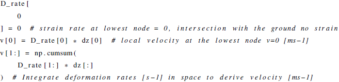The fact that the ice volume fraction stored at node k relates to the snow mass contained in the element above, whereas the strain rate calculated at node k is used for the deformation of the element below, leads to inconsistencies when ice volume fraction is updated. Therefore, we modified the code so that the strain rate used to deform the space interval between nodes k and k−1 during the mesh update step is the one evaluated at node k−1 instead of the one evaluated at node k. Concretely, the code lines reported above are replaced by the following:
.

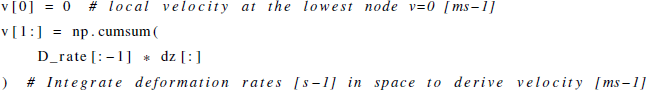D2 Inconsistency in the sequence of tasks

In the published version of the code, the strain rate was updated in between the ice volume fraction update and mesh update steps, leading to inconsistency between the two operations. This inconsistency was corrected by replacing the code lines

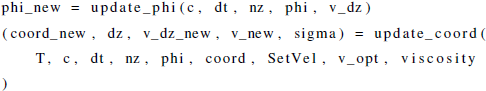
of the Model/coupled_update_phi_coord.py file (l. 13–16) with
.

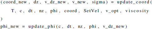D3 Inconsistency in the relationship between Φ_i and the effective snow density

In the code of Simson and Kowalski (2021), which is consistent with Eq. (18) of their article (Simson et al., 2021), the stress is calculated from the overburden snow mass neglecting the contribution of the air mass, i.e., assuming that the effective snow density is ρ_snow=ρ_iΦ_i. However, in the code, the initial field of the ice volume fraction ${\mathrm{\Phi }}_{\mathrm{i}}^{\mathrm{0}}$ is retrieved from the user-prescribed initial field of snow density ${\mathit{\rho }}_{\mathrm{snow}}^{\mathrm{0}}$ as follows:

$$\begin{array}{}\text{(D1)}& {\mathrm{\Phi }}_{\mathrm{i}}^{\mathrm{0}}={\displaystyle \frac{{\mathit{\rho }}_{\mathrm{snow}}^{\mathrm{0}}-{\mathit{\rho }}_{\mathrm{a}}}{{\mathit{\rho }}_{\mathrm{i}}-{\mathit{\rho }}_{\mathrm{a}}}},\end{array}$$

where ρ_a=1.335 kg m⁻³ is the air density. To correct this inconsistency, line 19 of the Model/phi_from_rho_eff.py file, which was
is replaced with
.

D4 Explicit vs. implicit time integration of the continuity equation

In the published version of the code, the continuity equation is discretized using an explicit time integration scheme. This is done in the Model/coupled_update_phi_coord.py file via the following code line: . Switching to the mass-conservative implicit time integration scheme implies replacing this code line with the following: .

Appendix E: Mass-conservative temporal discretization of the continuity equation

Let us consider the numerical layer $k+\mathrm{1}/\mathrm{2}$ undergoing settlement without any phase change between t and t+Δt. If we denote ${\mathrm{\Phi }}_{\mathrm{i},k+\mathrm{1}/\mathrm{2}}^n$ and $L_{k+\mathrm{1}/\mathrm{2}}^n$ (${\mathrm{\Phi }}_{\mathrm{i},k+\mathrm{1}/\mathrm{2}}^{n+\mathrm{1}}$ and $L_{k+\mathrm{1}/\mathrm{2}}^{n+\mathrm{1}}$), the ice volume fraction and length of the numerical layer before (after) settlement, and if we neglect the contribution of air in the snow mass, the mass conservation can be simply expressed as follows:

$$\begin{array}{}\text{(E1)}& {\mathrm{\Phi }}_{\mathrm{i},k+\mathrm{1}/\mathrm{2}}^{n+\mathrm{1}}{L}_{k+\mathrm{1}/\mathrm{2}}^{n+\mathrm{1}}={\mathrm{\Phi }}_{\mathrm{i},k+\mathrm{1}/\mathrm{2}}^n{L}_{k+\mathrm{1}/\mathrm{2}}^n,\end{array}$$

which can be rewritten as

$$\begin{array}{}\text{(E2)}& {\mathrm{\Phi }}_{\mathrm{i},k+\mathrm{1}/\mathrm{2}}^{n+\mathrm{1}}={\mathrm{\Phi }}_{\mathrm{i},k+\mathrm{1}/\mathrm{2}}^n{\displaystyle \frac{L_{k+\mathrm{1}/\mathrm{2}}^n}{L_{k+\mathrm{1}/\mathrm{2}}^{n+\mathrm{1}}}}.\end{array}$$

The total deformation of the layer $k+\mathrm{1}/\mathrm{2}$ over Δt is as follows:

$$\begin{array}{}\text{(E3)}& L_{k+\mathrm{1}/\mathrm{2}}^{n+\mathrm{1}}-L_{k+\mathrm{1}/\mathrm{2}}^n=\underset{z=z_k^n}{\overset{z_{k+\mathrm{1}}^n}{\int }}{\dot{\mathit{ϵ}}}_{zz}^{n+\mathrm{1}}\left(z\right)\mathrm{d}z\mathrm{\Delta }t.\end{array}$$

Thus, the spatially averaged strain can be expressed as follows:

$$\begin{array}{}\text{(E4)}& {\displaystyle \frac{L_{k+\mathrm{1}/\mathrm{2}}^{n+\mathrm{1}}-L_{k+\mathrm{1}/\mathrm{2}}^n}{L_{k+\mathrm{1}/\mathrm{2}}^n}}={\displaystyle \frac{{\int }_{z=z_k^n}^{z_{k+\mathrm{1}}^n}{\dot{\mathit{ϵ}}}_{zz}^n\left(z\right)\mathrm{d}z}{L_{k+\mathrm{1}/\mathrm{2}}^n}}\mathrm{\Delta }t={\dot{\mathit{ϵ}}}_{zz,k+\mathrm{1}/\mathrm{2}}^{n+\mathrm{1}}\mathrm{\Delta }t.\end{array}$$

It follows that

$$\begin{array}{}\text{(E5)}& {\displaystyle \frac{L_{k+\mathrm{1}/\mathrm{2}}^{n+\mathrm{1}}}{L_{k+\mathrm{1}/\mathrm{2}}^n}}=\mathrm{1}+{\dot{\mathit{ϵ}}}_{zz,k+\mathrm{1}/\mathrm{2}}^{n+\mathrm{1}}\mathrm{\Delta }t.\end{array}$$

Combining Eqs. (E2) and (E5) gives

$$\begin{array}{}\text{(E6)}& {\mathrm{\Phi }}_{\mathrm{i},k+\mathrm{1}/\mathrm{2}}^{n+\mathrm{1}}={\displaystyle \frac{{\mathrm{\Phi }}_{\mathrm{i},k+\mathrm{1}/\mathrm{2}}^n}{\mathrm{1}+{\dot{\mathit{ϵ}}}_{zz,k+\mathrm{1}/\mathrm{2}}^{n+\mathrm{1}}\mathrm{\Delta }t}}.\end{array}$$

Equation (E6) guarantees mass conservation by construction (provided that the air contribution in the snow mass is neglected). Equation (19) is an extension of Eq. (E6) that also includes the contribution of the mean deposition within layer $k+\mathrm{1}/\mathrm{2}$. When phase change is present, the deposition/sublimation effectively changes the ice volume fraction affected to the layer.