the Creative Commons Attribution 4.0 License.
the Creative Commons Attribution 4.0 License.
 | 01 Nov 2023
Description and performance of a sectional aerosol microphysical model in the Community Earth System Model (CESM2)
Michael J. Mills
Yunqian Zhu
Charles G. Bardeen
Francis Vitt
Pengfei Yu
David Fillmore
Xiaohong Liu
Brian Toon
Terry Deshler
We implemented the Community Aerosol and Radiation Model for Atmospheres (CARMA) in both the high- and low-top model versions of the Community Earth System Model Version 2 (CESM2). CARMA is a sectional microphysical model, which we use for aerosol in both the troposphere and stratosphere. CARMA is fully coupled to chemistry, clouds, radiation, and transport routines in CESM2. This development enables the comparison of simulations with a sectional (CARMA) and a modal (MAM4) aerosol microphysical model in the same modeling framework. The new implementation of CARMA has been adopted from previous work, with some additions that align with the current CESM2 Modal Aerosol Model (MAM4) implementation. The main updates include an interactive secondary organic aerosol description in CARMA, using the volatility basis set (VBS) approach, updated wet removal, and the use of transient emissions of aerosols and trace gases. In addition, we implemented an alternative aerosol nucleation scheme in CARMA, which is also used in MAM4. Detailed comparisons of stratospheric aerosol properties after the Mount Pinatubo eruption reveal the importance of prescribing sulfur injections in a larger region rather than in a single column to better represent the observed evolution of aerosols. Both CARMA and MAM4 in CESM2 are able to represent stratospheric and tropospheric aerosol properties reasonably well when compared to observations. Several differences in the performance of the two aerosol models show, in general, an improved representation of aerosols when using the sectional aerosol model in CESM2. These include a better representation of the aerosol size distribution after the Mount Pinatubo volcanic eruption in CARMA compared to MAM4. MAM4 produces on average smaller aerosols and less removal than CARMA, which results in a larger total mass. Both CARMA and MAM4 reproduce the stratospheric aerosol optical depth (AOD) within the error bar of the observations between 2001 and 2020, except for recent larger volcanic eruptions that are overestimated by both model configurations. The CARMA background surface area density and aerosol size distribution in the stratosphere and troposphere compare well to observations, with some underestimation of the Aitken-mode size range. MAM4 shows shortcomings in reproducing coarse-mode aerosol distributions in the stratosphere and troposphere. This work outlines additional development needs for CESM2 CARMA to improve the model compared to observations in both the troposphere and stratosphere.
- Article
(17245 KB) - Full-text XML
- BibTeX
- EndNote


Earth system models (ESMs) are necessary tools to understand the effects of natural and anthropogenic influences on the climate system in the past and present and are essential for the prediction of future changes. These models parameterize complex interactions between different Earth system components to be efficient enough to run on current supercomputer systems with reasonable throughput. A range of parameterizations with different complexity has been developed to reproduce physical processes reasonably well for specific scientific applications. To run long climate simulations, simplified schemes for chemistry and aerosols have been developed that perform well compared to observations (Danabasoglu et al., 2020). However, simplified schemes lack physical interactions, such as the coupling between aerosol and chemistry in the stratosphere, as included in a more comprehensive model configuration (Mills et al., 2016, 2017). More sophisticated parameterizations are necessary to understand the possible shortcomings in the simplified parameterizations and to reduce uncertainties in ESM predictions.
Here, we focus on the representation of aerosols in the troposphere and stratosphere. Aerosols play an important role in both climate (Kremser et al., 2016) and air quality (e.g., Fiore et al., 2015). Large uncertainties exist in aerosol formation, cloud and aerosol coupling, the effects on radiation and chemistry, and the removal of aerosols. Different aerosol schemes have been developed in ESMs, reaching from simplified bulk aerosol models with fixed sizes and externally mixed aerosols (e.g., Chin et al., 2002; Colarco et al., 2010) and modal representations of the aerosol distribution, assuming internally mixed aerosols within each mode (modal aerosol models; e.g., Liu et al., 2012), to the most complicated, size-resolved representation of the atmospheric aerosol distributions (also called sectional aerosol models; e.g., Kokkola et al., 2018; Sukhodolov et al., 2021). Depending on these representations, interactions between aerosols and other components (clouds, chemistry, and radiation) need to be adjusted to accommodate the specifics of the aerosol scheme.
The purpose of this work is to describe and evaluate the performance of a sectional aerosol model for both troposphere and stratosphere, following the implementation by Yu et al. (2015), into different atmospheric configurations of the Community Earth System Model Version 2 (CESM2). The sectional aerosol model used here is a configuration of the Community Aerosol and Radiation Model for Atmospheres (CARMA). CARMA is a framework for sectional aerosol models and is also referred to as a size-resolved cloud and aerosol model (Toon et al., 1988; Bardeen et al., 2008, 2013; Yu et al., 2015; Zhu et al., 2015, 2017; Yu et al., 2022). The CARMA aerosol model has been previously coupled to Community Earth System Model (CESM) Version 1 using the Community Atmospheric Model, versions 4 and 5 (CAM4 and CAM5), with tropospheric and stratospheric chemistry, which resulted in improved aerosol representation compared to a modal aerosol model based on various comparisons with observations (e.g., Yu et al., 2015, 2016, 2017; Murphy et al., 2021). In this study, we compare the two different aerosol models (CARMA and MAM4) using two CESM2 atmospheric configurations, namely CAM6, with comprehensive tropospheric and stratospheric chemistry (CAM6chem), and the Whole Atmosphere Community Climate Model Version 6, with middle-atmospheric chemistry (WACCM6-MA). These configurations include the coupling to chemistry, radiation, optics, cloud–aerosol interactions, emissions, and wet and dry removal.
The new implementation in CESM2, as discussed here, allows running the two available aerosol models (MAM4 and CARMA) within the same code base. Simulations with the same dynamical core, radiation scheme, chemistry, and transport scheme and with nudged meteorological fields, e.g., winds and temperatures, are performed to identify differences that are, for the most part, based on the aerosol scheme and related couplings. Some improvements to the Yu et al. (2015) CARMA aerosol model and the atmospheric coupling have been implemented to align it with some recent atmospheric model developments. These include updates in the wet removal scheme and the description of secondary organic aerosols (see Sect. 2.2). In addition, CARMA coupled to the high-top model WACCM6 (Gettelman et al., 2019; Davis et al., 2022) allows an improved representation of stratospheric transport and dynamics compared to the low-top model. In contrast to an earlier CARMA version coupled to WACCM4 (English et al., 2012), aerosols are radiatively active. In this paper, we evaluate aerosols and optical properties in the stratosphere and troposphere, including the impacts of small and large volcanic eruptions and the aerosol background composition, based on in situ and satellite observations. The effects on chemistry are only briefly evaluated. The implementation of the optional sectional aerosol model CARMA in the atmospheric model of CESM2 and its evaluation is the first step towards a fully coupled CESM2 CARMA configuration, including ocean and sea ice, which will allow fully coupled climate simulations.
The paper is organized as follows. Details of the model and the two aerosol microphysical schemes used are given in Sect. 2. This also includes details of the coupling between CESM2 and CARMA or MAM4 with regard to various processes covering cloud–aerosol interactions, dry and wet removal, radiation and optics, chemistry, and emissions. We further outline the computational performance of the different configurations used in this work. Section 3 describes the experimental design of the work. Results of the stratospheric aerosol performance are summarized in Sect. 4, with details on the performance of the model simulation of the aerosol evolution after the Mount Pinatubo volcanic eruption, based on sensitivity tests. Background stratospheric aerosol properties and ozone are also evaluated. Section 5 focuses on the tropospheric aerosol model performance between 2001–2020 and between 2016 and 2018 compared to the NASA Atmospheric Tomography Mission (ATom). We close with a discussion and suggestions for further model development in Sect. 6 and conclude thereafter.
2.1 CESM2.2 model configurations
Experiments performed in this study are based on two different atmospheric configurations, CAM6chem and WACCM6-MA of the Community Earth System Model (CESM2.2; Danabasoglu et al., 2020). CAM6chem includes comprehensive chemistry in the troposphere and stratosphere (TS1; Emmons et al., 2020), with some minor updates added in this study, and uses a configuration with 0.9∘ × 1.25∘ in the horizontal resolution and 32 levels in the vertical, with a top at around 42 km. The aerosol model includes a volatility basis set (VBS) secondary organic aerosol scheme (Tilmes et al., 2019), including interactive biogenic emissions from the Model of Emissions of Gases and Aerosols from Nature version 2.1 (MEGAN2.1; Guenther et al., 2012). This model version is frequently used for air quality studies in the troposphere (e.g., Gaubert et al., 2021; Tang et al., 2022) and for studies in the upper troposphere and lower stratosphere (UTLS). It also performs well when compared to observations in the stratosphere (Emmons et al., 2020).
WACCM-MA is a high-top version of CESM and has 70 vertical levels, with a model top at about 150 km. It has been designed for studies that focus on stratospheric chemistry and circulation, including impacts of volcanic eruptions and stratospheric aerosol injection. For example, the first Geoengineering Large Ensemble Simulations (GLENS; Tilmes et al., 2018) used an earlier WACCM-MA version with 0.9∘ × 1.25∘ horizontal resolution. In this work, we use CESM2(WACCM-MA) with 1.9∘ × 2.5∘ horizontal resolution (Davis et al., 2022). This model version, coupled with a full ocean, shows a reasonable climate response, and its dynamics and chemistry in the stratosphere are comparable to the 0.9∘ × 1.25∘ WACCM6 version with comprehensive tropospheric and stratospheric chemistry. The model includes comprehensive chemistry in the stratosphere, mesosphere, and lower thermosphere but only represents chemistry with limited complexity in the troposphere (Davis et al., 2022). In turn, secondary organic aerosols (SOAs) are only represented in a simplified manner.
2.2 Standard aerosol description in CESM2 using the Modal Aerosol Model (MAM4)
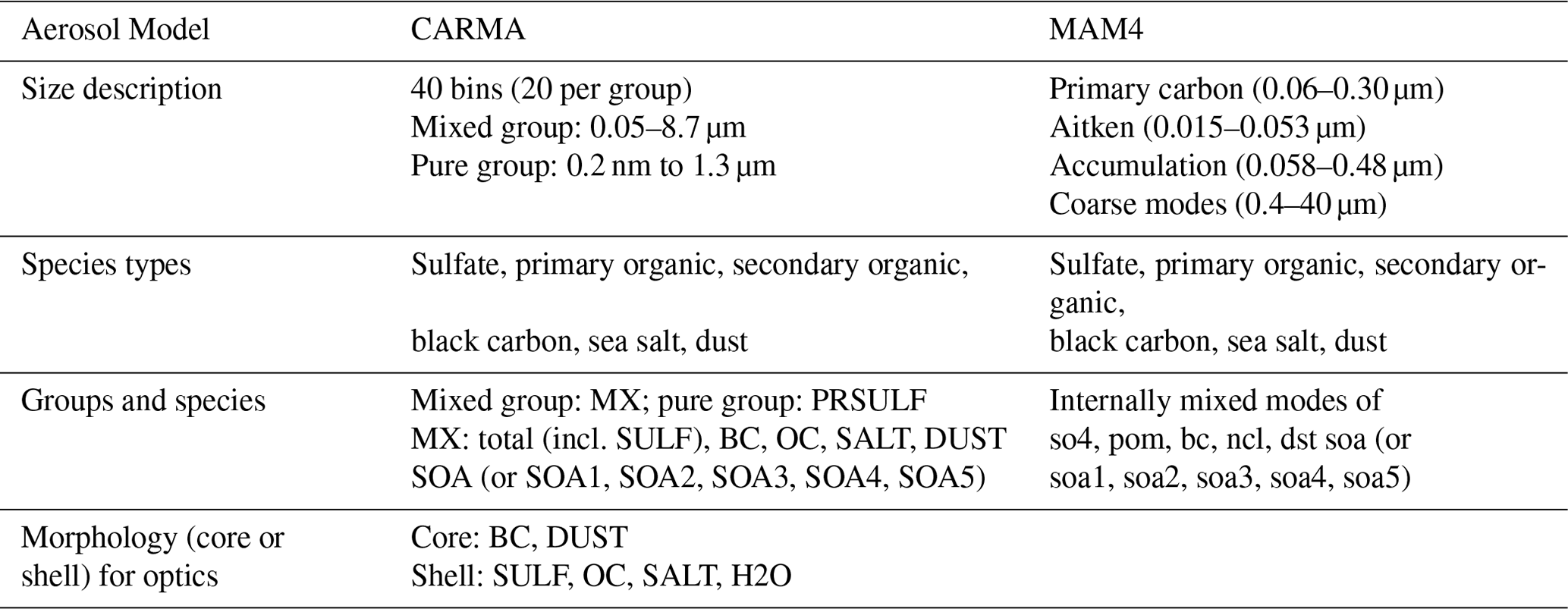
The default CESM2 aerosol scheme in CAM6chem and WACCM6 is the Modal Aerosol Model (MAM4; Liu et al., 2012, 2016), with updated prognostic stratospheric sulfate aerosols (Mills et al., 2016). MAM4 microphysics describes four modes, namely the Aitken, accumulation, coarse, and primary carbon modes. The primary carbon mode has been added to represent the aging processes of black carbon and primary organic matter, while being coated by soluble species (sulfate and organics) with monolayers (Liu et al., 2016). The geometric standard deviation in MAM4 for the different modes is Aitken at 1.6, accumulation at 1.6, primary carbon mode at 1.6, and coarse at 1.2 (Liu et al., 2016; Mills et al., 2016). The relatively small sigma value of 1.2 for the coarse mode had been chosen to accommodate the stratospheric coarse-mode sulfate, following Niemeier et al. (2011). Table 1 describes the model settings of the size range, particle types, and morphology for MAM4 and CARMA aerosols.
The microphysics of MAM4 include a binary parameterization (Vehkamäki et al., 2002) for the sulfuric acid vapor (H2SO4-H2O) homogeneous nucleation for new particle formation. The loss of the new particles by coagulation, as they grow from a critical cluster size to the Aitken-mode size, is accounted for using the parameterization by Kerminen and Kulmala (2002). The condensation of H2SO4 vapor is treated dynamically, using a standard mass transfer expression that is integrated over the size distribution of each mode (Binkowski and Shankar, 1995). An accommodation coefficient of 0.65 is used for H2SO4 and other species (Pöschl et al., 1998). In the troposphere, H2SO4 condensation is treated as irreversible, while SOA (gas) condensation is reversible and based on equilibrium vapor pressure over particles. The evaporation of sulfate particles is included only above the tropopause (Mills et al., 2016). The coagulation of the Aitken, accumulation, and primary carbon modes is treated within each and between different modes. It reduces the number but leaves the mass unchanged. For tropospheric aerosol, water uptake in MAM4 is based on the equilibrium Köhler theory (Ghan and Zaveri, 2007), using the relative humidity and the volume mean hygroscopicity for each mode to diagnose the wet volume mean radius of the mode from the dry volume mean radius. Gravitational settling velocities are calculated as a function of altitude (Seinfeld and Pandis, 1998). For the stratosphere, sulfates are in equilibrium with the water. The water uptake (and therefore the weight percentage of H2SO4) is calculated based on the parameterization by Tabazadeh et al. (1997). Settling velocities depend on wet particle size and mass and are, therefore, different between modes.
2.3 Community Aerosol and Radiation Model for Atmospheres (CARMA)
The CARMA aerosol model (version 4.3) for the troposphere and stratosphere (denoted CARMA in the following) includes prognostic aerosols in both the troposphere and stratosphere, as described in detail in Yu et al. (2015). The implementation is further based on previous aerosol descriptions for sea salt (Fan and Toon, 2011), dust storms (Su and Toon, 2009), and stratospheric sulfates (English et al., 2013). Additional implementations, such as the inclusion of volcanic ash (Zhu et al., 2020), new descriptions of polar stratospheric clouds (PSCs; Zhu et al., 2015, 2017), polar mesospheric clouds (PMCs; Bardeen et al., 2010), and sectional nitrate and ammonium (Yu et al., 2022), are not included in the current version of the model but will be included in future work.
CARMA can be configured with numerous classes of particles or groups. We employ an internally mixed group composed of primary and secondary organics, black carbon, sulfate, dust, and sea salt, as well as a pure sulfate group that only includes sulfates (see Table 1). The pure sulfate group includes the nucleation of H2SO4, condensation, and coagulation with both the pure and mixed groups. The pure sulfate group can be used to identify geographic regions of active nucleation. CARMA keeps track of the total mass and the core masses (or elements) of each group in each mass bin, with sulfuric acid acting as the volatile component of each bin. Currently, CARMA only allows one component of a group to be volatile, which is sulfate for the mixed and pure aerosol groups. The volatility of SOA (gas-to-aerosol exchange) is therefore calculated in the chemistry module in CAM, and the resulting rates are passed into CARMA. Each group is described as individual discrete aerosol mass bins. Here, we use 20 mass bins, as defined in Yu et al. (2015). The bins track the dry mass of the particles and assume that water is in equilibrium to calculate the wet radius of the particle. The mixed aerosol group defines these bins between 0.05–8.7 µm in radius and the pure sulfate group from 0.2 nm to 1.3 µm. In addition, CARMA is capable of resolving many more arbitrary distributions of aerosol sizes, in contrast to the minimalist approach of MAM4, which assumes a superposition of only four lognormal modes (with two of those, the primary carbon mode and the accumulation mode, covering very similar size ranges).
Microphysical processes in CARMA include the binary homogeneous nucleation of sulfuric acid and water (Zhao and Turco, 1995; called the Zhao scheme in the following) and sulfuric acid evaporation (Toon et al., 1989) for the pure sulfate group only; sulfuric acid condensation and gravitational settling for both groups; and aerosol coagulation within and between the mixed and pure groups, including the effects of Van der Waals forces (English et al., 2011). In addition to the Zhao scheme, in this work, we added the binary homogeneous nucleation scheme (called the Vehkamäki scheme in the following), as described in Vehkamäki et al. (2002). This nucleation scheme is also used in MAM4 as the default. Vehkamäki et al. (2002) employ an improved model for hydrate formation that is valid for both tropospheric and stratospheric conditions and uses a parameterization based on observations. In contrast, the Zhao scheme is based on a physical approach and was developed and validated primarily for stratospheric conditions. The effects of the two schemes are compared for the Mount Pinatubo eruption in 1991 (Sect. 4.1.2.) and for tropospheric background conditions (Sect. 5.2.4.). The model does not currently employ nucleation influenced by ammonia or organics, which is important for radiation and other aerosol processes (Lu et al., 2021).
For the pure sulfate group, as for MAM4 in the stratosphere, the wet radius of the particle is determined by the weight percent of H2SO4 in the particles, based on the parameterization by Tabazadeh et al. (1997). For the mixed radius, the wet radius is parameterized based on the relative humidity and the weighted hygroscopicity, while also considering the composition of the internally mixed particles (Petters and Kreidenweis, 2007). To avoid generating particles that are too large through swelling, relative humidity is constrained to be less than 99.5 % in CARMA when calculating the wet radius and wet density of particles. While Yu et al. (2015) assumed no particle swelling below 190 K, in this study, we use the relative humidity at 190 K to calculate the particle swelling and the wet radius below 190 K. CARMA further includes the parameterization of emissions of sea salt and dust, as well as the removal of aerosols through wet and dry deposition that can be independent of the atmospheric model configuration (as described in Sect. 2.4.5).
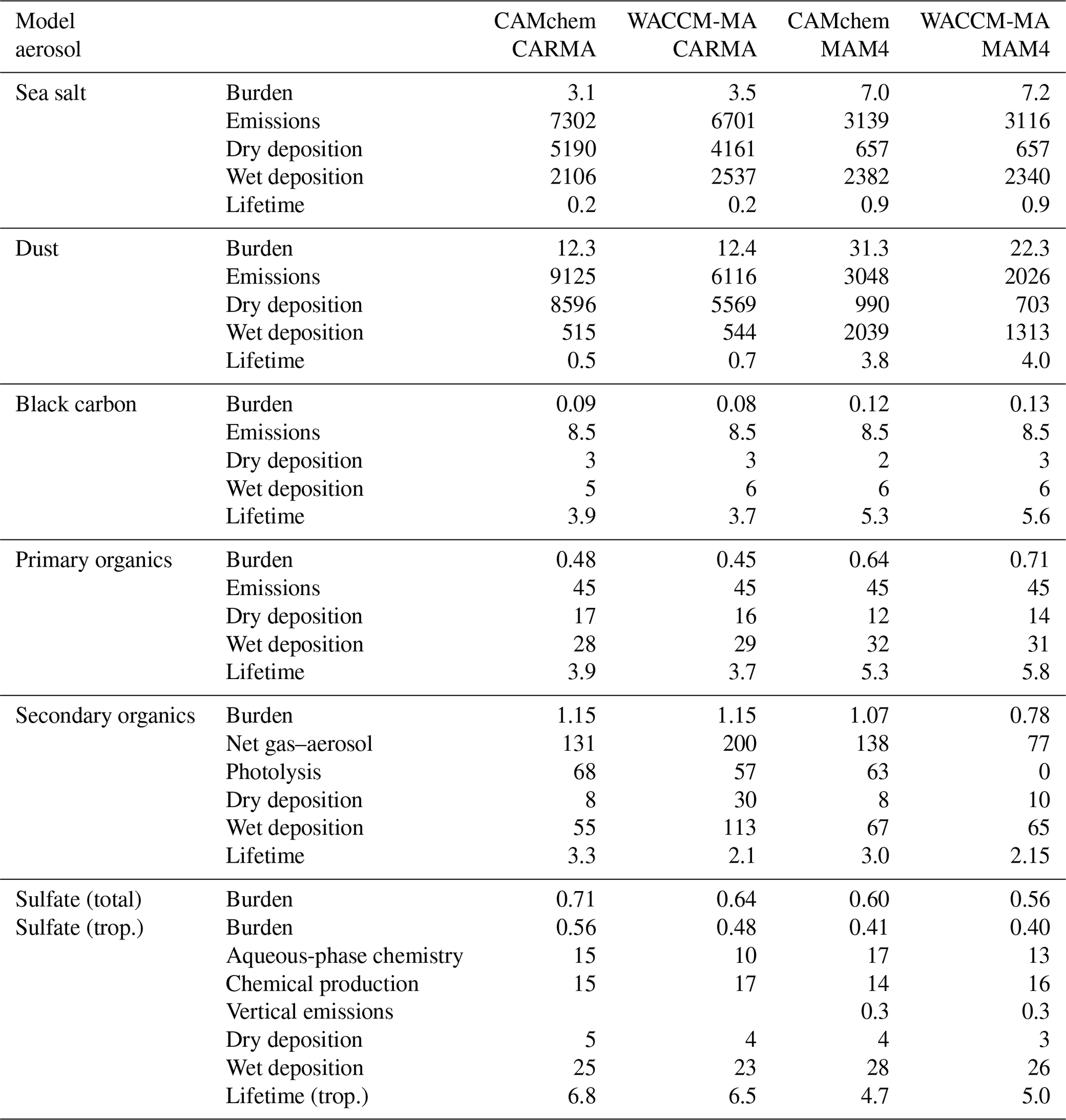
Table 1Aerosol specifics for CARMA and MAM4 aerosol microphysical models coupled to WACCM-MA and CAM6chem. The species names used here are specific to each aerosol model.
2.4 Coupling between CESM2 and CARMA or MAM4
Aerosols interact with various processes in the atmosphere and need to be coupled to those components of the atmospheric model independent of the aerosol scheme. These processes include radiation and optics, chemistry–aerosol interactions, cloud–aerosol interactions, emissions, and wet and dry deposition, as illustrated in Fig. 1. MAM4 aerosol microphysical processes are integrated into the workflow of the CESM2 atmospheric model. In contrast, CARMA has been integrated as a standalone model, resulting in a slightly different ordering than MAM4. The order of applied physical processes is indicated as numbers black for MAM4 and red for CARMA in Fig. 1.
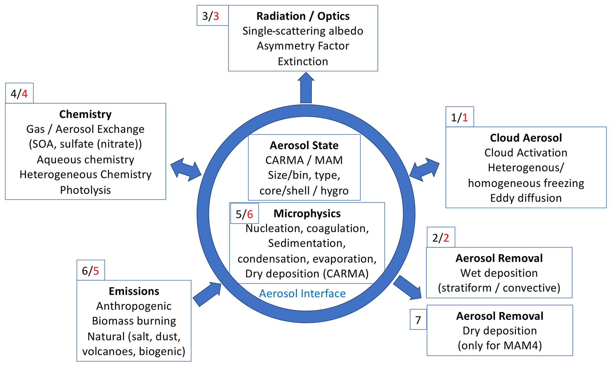
Figure 1Schematic of the coupling between different aerosol processes and CAM6chem and WACCM-MA. The order of processes related to aerosols in CESM2–CAM6 is illustrated in small numbers (black for MAM4 and red for CARMA) given in each process box. The blue circle separates the processes that occur as part of the aerosol microphysical scheme from the processes that are specific to the atmospheric model (CAM6).
Physical processes within the Community Atmospheric Model (CAM) are split according to time, meaning that processes happen sequentially in a specified order rather than all at once (Williamson, 2002). Physical processes are divided between processes that occur before coupling and after coupling with surface processes (e.g., land and ocean). The processes before coupling, besides advection and convection (not included in Fig. 1), include deep convection (Zhang and McFarlane, 1995), planetary boundary layer processes, shallow convection, and moist turbulence (Bogenschutz et al., 2012). These are coupled to aerosol activation (Abdul-Razzak and Ghan, 2000), eddy diffusion (Process 1 in Fig. 1), two-moment cloud microphysics (Gettelman and Morrison, 2015), and convective and stratiform wet removal (Process 2 in Fig. 1). After that, optical properties and radiative transfer are calculated (Process 3 in Fig. 1), followed by the coupling to the land and ocean.
In CAM6, surface emission fluxes for gases and aerosol, including anthropogenic, biomass burning, biogenic, and ocean emissions, are calculated after the surface coupling. However, they are added to the lower atmospheric layer after chemistry. Chemistry (Process 4) includes aqueous-phase chemistry and gas–aerosol exchange and applies vertical emissions of gases and aerosol. Chemistry also includes the MAM4 microphysical processes (Process 5 for MAM4). After chemistry, the emissions are applied (Process 6), followed by the dry removal of gases, including aerosol precursors like sulfur and volatile organic compounds (VOCs; not shown in Fig. 1). Finally, dry deposition of aerosol is applied (Process 7 for MAM4). For CARMA, microphysical processes are not included in chemistry but are applied later. In this case, emissions of gases and aerosols (Process 5 for CARMA) and dry deposition of gases (not shown in Fig. 1) are applied after chemistry. Aerosol microphysics for CARMA (Process 6) is done last, which includes sedimentation, dry deposition, molecular diffusion, and coagulation, followed by nucleation, growth, and evaporation. The calculation of nucleation, growth, and evaporation rates are performed simultaneously and undergo convergence checks to make sure that the gas concentration (here H2SO4) is not negative and that temperature and supersaturation changes do not exceed predefined thresholds. If convergence cannot be reached due to large process rates, the model will retry with shorter substeps until convergence is reached. This will result in a stable solution for each modeled time step. The substepping will add some processing time to the model, particularly during a spin-up phase when gases and aerosols have not reached sufficient balance.
Aerosol microphysics for CARMA (Process 6) is done last, which includes sedimentation, dry deposition, molecular diffusion, and coagulation, followed by nucleation, growth, and evaporation, which may be substepped for stability due to potentially large process rates.
2.4.1 Cloud–aerosol processes
Advected aerosols in the atmosphere (for modal and sectional models in CAM6) are called interstitial aerosols. The aerosols that have been activated to serve as condensation nuclei and form clouds are removed from the interstitial aerosols and are classified as the so-called cloud-borne aerosols (Easter et al., 2004). Cloud-borne aerosols in CAM6 (both MAM4 and CARMA) are not advected. The transition between interstitial and cloud-borne aerosols, and vice versa, depends on the atmospheric conditions, including ice and liquid cloud fraction, relative humidity, and temperature.
The activation of clouds is calculated for both MAM4 and CARMA, based on the critical supersaturation of air masses, which is obtained from the turbulent vertical velocity in the updraft of air masses (Abdul-Razzak and Ghan, 2000). The turbulent vertical velocity is based on subgrid processes and is currently parameterized and represented through a probability distribution function. In addition to the aerosol activation, diffusive mixing of aerosols across vertical levels has been considered for both MAM4 and CARMA. Shrinking or removing clouds leads to the evaporation of cloud-borne aerosols in the model, which moves them back into interstitial aerosols. In MAM4, this method is applied for each lognormal mode and each species, and in CARMA it is applied for all bins and species per bin. Both MAM4 and CARMA keep track of cloud-borne particles for each mode and bin they originated from when activated. After the evaporation of clouds, aerosols are moved back into the mode or bin of their origin.
Both homogeneous and heterogeneous nucleation is considered in MAM4 and CARMA for ice crystal nucleation in mixed-phase and cirrus clouds. It is based on the particle number of dust and sulfate within the mixed and the pure sulfate group in CARMA, considering only aerosols that are >0.1 µm. For MAM4, the Aitken mode of sulfate and coarse mode of dust are considered for ice nucleation in ice clouds (Liu and Penner, 2005; Liu et al., 2007). For CARMA, nucleation, condensation, and deposition in mixed clouds ∘C are done based on Mayers et al. (1992). In contrast, MAM4 describes the heterogeneous nucleation in mixed-phase clouds based on the classical nucleation theory described in Wang et al. (2014).
2.4.2 Dry and wet removal of aerosols
The wet removal of aerosols, including in-cloud and below-cloud wet removal, is done by coupling to the atmospheric model (CAM6). In CAM6, in-cloud removal in shallow convective and stratiform clouds is treated seamlessly, based on the cloud and precipitation information from the two-moment Morrison–Gettelman microphysics (Gettelman and Morrison, 2015). For the wet removal in deep convective clouds, CAM6 uses the Zhang and McFarlane (1995) deep convection scheme coupled with a unified scheme for aerosol convective transport and wet scavenging by Wang et al. (2013), with updates and improvements by Shan et al. (2021). For CARMA, we also adopt the convective wet removal scheme by Wang et al. (2013) and Shan et al. (2021). An updated version of CESM1–CARMA adopted a different convective removal scheme introduced by Yu et al. (2019), which also considers the secondary activation of aerosols from entrained air above the cloud base.
Aerosol dry deposition velocities in MAM4 and CARMA are calculated using the Zhang (2001) parameterization with prescribed land use and surface layer information. Aerosol mixing ratio changes and fluxes from dry deposition and sedimentation are calculated throughout a vertical column. Differences in dry deposition fluxes between MAM4 and CARMA (see below) are due to the differences in the particle size of the mixed group, which results in larger particles and faster sedimentation for CARMA compared to MAM4, as also discussed in Yu et al. (2015).
2.4.3 Radiative transfer and optics
CAM6 uses the rapid radiative transfer model for general circulation models (RRTMG; Iacono et al., 2008) for the radiative transfer calculation in the longwave (16 bands) and shortwave (14 bands) range, including heating rates and radiative fluxes. Besides using the information on cloud fraction from liquid, ice, and snow, it requires information on aerosol extinction, single-scattering albedo, and asymmetry parameter per wavelength band in the shortwave and absorption in both long- and shortwave bands. For CARMA, the integration of optics for a core shell representation that has been included for the mixed particle by Yu et al. (2015) is adopted here, using lookup tables that include precalculated aerosol radiative properties based on the Mie theory and following the core shell assumption by Toon and Ackerman (1981). Black carbon and dust are assumed to form the core of the mixed particles, while the other water-soluble constituents form the shell. Here, we expand the radiative properties to consider secondary organic aerosols using the lookup tables derived for organic aerosols (Yu et al., 2015). MAM4 uses the parameterization by Ghan and Zaveri (2007) that assumes an internal mixture of hydrated aerosol components with lognormal size distributions to calculate optical properties using the wet-surface-mode radius. As for CARMA, precalculated aerosol properties based on the Mie theory are provided through lookup tables.
2.4.4 Coupling of aerosols to CESM2 chemistry
CAM6chem and WACCM6-MA (called CAMchem and WACCM-MA in the following) include interactive chemistry in the troposphere and stratosphere. WACCM-MA includes much more simplified tropospheric chemistry, resulting in less ozone and other oxidants than CAMchem (Gettelman et al., 2019; Davis et al., 2022). Oxidants (in particular OH and ozone) are important for the formation of aerosol precursors (VOCs and SO2) for both SOA and sulfate. Detailed sulfur chemistry includes dimethyl sulfide (DMS), and organic carbonyl sulfide (OCS) as important precursor emissions for the troposphere and stratosphere (Mills et al., 2016).
The formation of sulfate in the troposphere through aqueous-phase chemistry is included for MAM4 and CARMA, as described in Barth et al. (2000). Aqueous-phase reactions include reactions of aqueous sulfur by ozone and hydrogen peroxide to form SO4 and therefore depend on tropospheric chemistry. The produced sulfate is added into the cloud-borne aerosol MAM4 sulfate modes or CARMA bins proportional to sulfur mass in each bin. The reduced oxidants in WACCM-MA are expected to lead to reduced aqueous-phase production, which generally results in larger sulfate burdens, since cloud-borne sulfate is removed faster than interstitial aerosols (Barth et al., 2000). In this version of the model, we updated aqueous-phase chemistry to only be active in liquid clouds. CAM6 also included reactions on ice clouds (not used here), which have not been sufficiently established in the literature.
The formation of SOA from aerosol precursors is performed differently in CAMchem and WACCM-MA. The formation of SOA in CAM-chem is based on the volatility basis set approach that defines five different SOA gas-phase and aerosol species that experience gas-to-aerosol exchange, depending on their volatility characteristics (Hodzic et al., 2016; Tilmes et al., 2019). For WACCM-MA, a simplified SOA scheme is used where a gaseous SOA precursor is directly emitted at the surface, and only one volatility bin is considered. Depending on the chemistry in the troposphere, either one (for simplified tropospheric chemistry in WACCM-MA) or five (for CAM-chem) elements have been added to the CARMA mixed aerosol group to represent the volatility bins and, therefore, the condensed phase of SOA in the bin. The additional SOA elements are fully coupled to CARMA microphysics and are part of the mixed particle (or group). The production and loss of SOA for each element are applied to the CARMA SOA aerosols. We also include SOA photolysis as a sink of SOA in the upper troposphere, assuming a reaction rate that is 0.04 times the photolysis rate of nitrogen dioxide, as discussed in Hodzic et al. (2015), and add the SOA formation from glyoxal in aqueous aerosols (Knote et al., 2014), as also done for MAM4 in CAMchem. For WACCM-MA, only CARMA includes the photolysis of SOA, while MAM4 does not.
Aerosols in both the troposphere and stratosphere further provide surfaces for heterogeneous reactions, e.g., affecting chemical reactions. In the troposphere, surface area density affecting heterogeneous reactions is calculated based on the mass and effective radius of sulfate, organic aerosols, and black carbon. For MAM4, the primary carbon mode (black carbon and primary organic matter) is not included in heterogeneous chemistry (Tilmes et al., 2015). In the stratosphere, both MAM4 and CARMA include the surface area density for six heterogeneous reactions, with varying rates for sulfate, nitric acid trihydrate, and water ice (Mills et al., 2016).
2.4.5 Emissions of aerosols
Surface and vertical emissions for anthropogenic, biomass burning, soil, and volcanic gases are prescribed for all experiments (see Sect. 3). The oceanic fluxes of DMS are calculated using the Online Air-‐Sea Interface for Soluble Species (OASISS; Jo et al., 2023). Dust and sea salt emissions are calculated as part of the aerosol model. CARMA uses size-dependent dust and sea salt source functions, which are described in detail in Yu et al. (2015). Briefly, the calculation of sea salt and dust emissions is based on 10 m winds from the atmospheric model and applies a Weibull wind distribution (Gillette and Passi, 1988) to represent the subgrid wind velocity. For the calculation of sea salt emissions, we use the sea spray aerosol source function introduced by Fan and Toon (2011), which combines different source functions for different aerosol size ranges. In contrast to Yu et al. (2015), marine organic aerosols are not included in CARMA to be consistent with MAM4. We use a 1 × 1∘ fixed soil erodibility file to calculate dust emissions and apply a dust emission scaling factor of 0.5 for the 1∘ CAMchem version and 0.4 for WACCM-MA.
MAM4 sea salt and dust emission fluxes are described in Liu et al. (2012), with updates for the dust emission size distributions. The sea salt emissions are based on the scheme by Mårtensson et al. (2003), derived for the dry diameter (Dp) <2.8 µm, and the (Monahan et al., 1986) scheme, derived for Dp > 2.8 µm, both of which depend on the 10 m wind, with the former also depending on ocean water temperature. The dust emissions are calculated, following the scheme of Zender (2003), with the emission size distribution calculation updated to be based on Kok (2011).
CARMA and MAM4 emissions are calculated as mass emission fluxes and are distributed over all the mass bins or modes, respectively. CARMA emits increasingly more mass into larger bins for sea salt and dust. This results in the relatively large total emissions in CARMA and consequently larger dry deposition due to larger deposition rates of larger particles, as discussed below (Sect. 5.2.1).
2.5 Computational performance
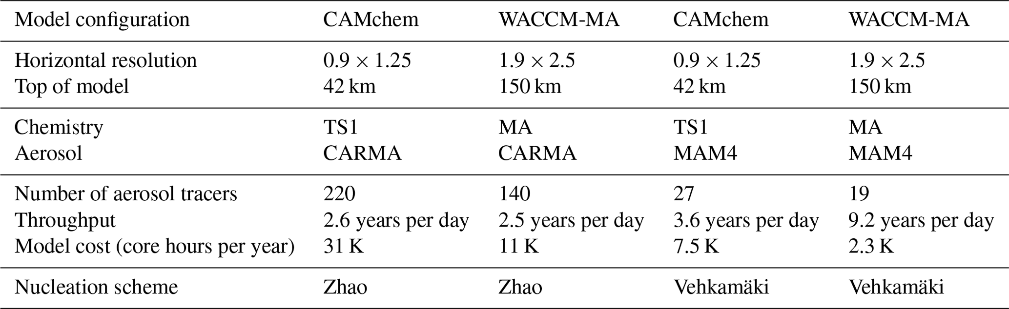
The CARMA size-resolving aerosol model includes 193 additional advected aerosol tracers for CAMchem and 121 for WACCM-MA (Table 2). The increase in advected tracers in CARMA compared to the Modal Aerosol Model configuration adds significantly to the computational costs of the atmospheric host model. Using CAMchem with 0.9∘ × 1.25∘ horizontal resolution increases the model costs from ≈7500 core hours per year (for MAM4) to ≈31 000 core hours per year of simulation for CARMA, with a smaller throughput for CARMA in the specific configuration. WACCM-MA, using 1.9∘ × 2.5∘ horizontal resolution, requires 11 000 core hours per year for CARMA. In comparison, the MAM4 configurations used here require 2300 core hours per year, including a much better throughput of 9.2 years per day of simulation in MAM4, compared to 2.5 years per day for CARMA.
Due to the long runtime, the CARMA model configurations need to be carefully chosen regarding the scientific needs and model costs. With the current configurations, decade-long simulations are easily possible. For studies of aerosols in the troposphere and UTLS, and to study the impacts of pyrocumulonimbus (pyroCb) events, the low-top CAMchem has been used successfully in the past (e.g., Yu et al., 2019). Complex tropospheric chemistry is required for tropospheric aerosol formation, which affects the aerosol burden, including secondary organic aerosols. A higher horizontal resolution is desired to better simulate the effects of meteorological variability and climate impacts. Tropospheric aerosol formation and composition may also be essential to investigate stratospheric background aerosol, since tropospheric aerosols and their precursors are naturally injected into the stratosphere, for example, through the upper tropical troposphere and the Asian monsoon anticyclone. They may also matter for evaluating solar-powered lofting experiments (Gao et al., 2021). On the other hand, the WACCM-MA configuration is more suited for stratospheric-focused experiments, including investigating the effects of volcanic eruptions or stratospheric aerosol injections on stratospheric chemistry and dynamics. However, this configuration, while relatively cheap, does not produce an interactive quasi-biennial oscillation (QBO) and may therefore not be optimal for specific research questions. Other configurations may be used, including WACCM-MA with a one-degree horizontal resolution, but its current model costs are around 70 000 core hours per simulated year. Even more expensive is the WACCM6 1∘ model version with full tropospheric and stratospheric chemistry (not evaluated here).
Table 2Model configurations and experiments between 2001 and 2020. Model costs are described in thousands (K) of core hours per year.
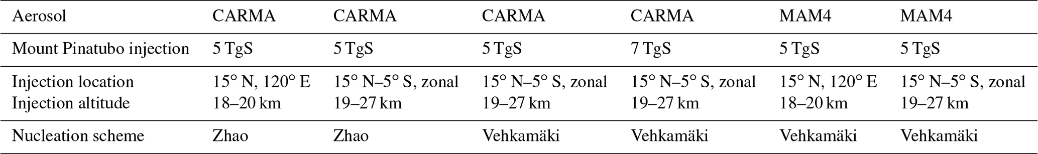
Two sets of model experiments are performed using different configurations of CESM2. All the model simulations use observed sea surface temperatures and sea ice conditions and are nudged every 12 h to winds and temperatures using Modern-Era Retrospective analysis for Research and Applications, version 2 (MERRA-2), meteorological reanalyses (Davis et al., 2022). The first set of experiments between 1990 and 1995 focuses on the period shortly before and after the largest recent volcanic eruption of Mount Pinatubo in June 1991 (Table 3). Here, different model experiments are compared, using WACCM-MA with CARMA and MAM4, in Sect. 2.1 (using 1.9∘ × 2.5∘ degrees (or “2deg”) horizontal resolution). The model simulations start from a historical WACCM-MA 2deg simulation in 1990. For CARMA, a 3-year spin-up period was added to properly build up background aerosols. The second set of experiments focuses on the performance of stratospheric background aerosol conditions, the effects of small volcanoes between 2001 and 2020, and the performance of tropospheric aerosol properties (Table 2). WACCM-MA simulations continued after 1995 (from the first set of experiments) for CARMA and MAM4. CAMchem configurations (using 0.9∘ × 1.25∘ degrees (or “1deg”) horizontal resolution; see Sect. 2.1) were started, using initial conditions taken from the historical WACCM6 Coupled Model Intercomparison Project Phase 6 (CMIP6) simulations.
Between 1990 and 2000, we use the CMIP6 emissions for anthropogenic, biomass burning, and soil and ocean emissions (Gettelman et al., 2019). Sulfur emissions for explosive volcanic eruptions are based on version 3.11 of Volcanic Emissions for Earth System Models (VolcanEESM; Neely and Schmidt, 2016). For Mount Pinatubo, we tested an updated SO2 injection profile over a larger region and time window than previously used. The new sulfur injection file has been developed because it reproduces observations better, as described in Sect. 4.1. In addition, sensitivity simulations using CARMA have been performed to evaluate the differences between the two nucleation schemes used in CARMA and MAM4 and larger sulfur injection amounts that show improved agreement with observations (Fisher et al., 2019). For the period between 2001 and 2020, we use CAMSv5.1 anthropogenic emissions and biomass burning emissions derived from Quick Fire Emissions Dataset (QFED) CO2 fields (Darmenov et al., 2015), multiplied by the species emissions factors collated in Fire INventory from NCAR Version 1.5 (https://www.acom.ucar.edu/Data/fire/, last access: 27 October 2023; Wiedinmyer et al., 2011). As described above, DMS ocean emissions, sea salt, and dust emissions are derived internally for WACCM-MA and CAMchem.
The Mount Pinatubo volcanic eruption in June 1991 was the largest eruption within the last 50 years and is often used to evaluate the performance of ESMs. Stratospheric aerosol optical depth and extinction from satellite observations are available over this period and are therefore useful measures to test the production and evolution of stratospheric aerosol in the model for a given injection of SO2 after Mount Pinatubo and also for other smaller eruptions. However, uncertainties exist in the total amount of sulfur injection after volcanic eruptions. Mills et al. (2016) and Mills et al. (2017) have found that the best agreement with optical observations following the Mount Pinatubo eruption using a modal aerosol model occurs with an injection of 10 Tg of SO2. Direct observations (e.g., Fisher et al., 2019), on the other hand, suggest that 12–13 Tg of SO2 were present as late as 6 d after the eruption. Carn et al. (2016) argue that to find the proper injection amount, one must extrapolate the SO2 back to the initial injection date, yielding as much as 17–19 Tg of SO2 injected. Unfortunately, the chemistry converting SO2 to sulfate and gas-phase reactions that can recycle vapor-phase H2SO4 back to SO2 are uncertain, especially in the first few days due to heterogeneous reactions on ash, which are often not included in models (Zhu et al., 2020). Furthermore, the resolution of ESMs is too coarse to resolve the small-scale plume evolution and the dilution of injected materials in the first day or two, which influences aerosol microphysical processes. Given the lack of heterogeneous chemistry on ash in these models, it is difficult to know how much sulfate aerosol was created by gas-phase SO2 chemistry and therefore exactly how many sulfur injections should be used for such a model.
Here, we investigate different model experiments using both aerosol microphysical schemes (MAM4 and CARMA) in the same WACCM-MA setup and different injection amounts, locations, altitude ranges, and aerosol nucleation schemes (see Table 3). Model results are compared to the stratospheric aerosol optical depth (SAOD) and aerosol extinction at 525 nm wavelength from the Global Space-based Stratospheric Aerosol Climatology (GloSSAC) for stratosphere aerosol properties (Thomason et al., 2018; Figs. 2, 3, and 6). In addition, we compare the SAOD from the Advanced Very High Resolution Radiometer/2 (AVHRR/2) spaceborne sensor to the model simulations, which was gridded on a grid and averaged over different months, as described in Quaglia et al. (2023). Since AVHRR/2 mainly covers the tropics and has limited coverage between 70∘ N and 70∘ S, we are not using the data for comparisons of mid- to high-latitude averages (Figs. 2 and 6). As discussed in earlier work (e.g., English et al., 2012), the GloSSAC dataset underestimates the SAOD in the first few months after the eruption compared to AVHRR/2.
4.1 Importance of the details of Mount Pinatubo injection locations
Recent model studies using MAM4 (e.g., Mills et al., 2016, 2017; Gettelman et al., 2019) used a single-column SO2 injection profile to simulate the Mount Pinatubo eruption and injected 5 TgS (equivalent to 10 Tg SO2) between 18 and 20 km at 15∘ N and 120∘ E on 15 June 1991. This injection amount was utilized to maximize the agreement between global aerosol optical properties using WACCM6 MAM4 and observations, while recent observational studies suggest larger injection amounts (see above). As expected, when using the same injection profile for WACCM-MA with MAM4 (Fig. 2a; red line), the global distribution of the SAOD is within the range of the standard deviation of the GloSSAC and AVHRR/2 observations, which is averaged between 80∘ N and 80∘ S. However, there is a significant underestimation of the SAOD in the Southern Hemisphere (SH; Fig. 2c; red line), while the Northern Hemisphere (NH) values are within the error bar of the observations. On the other hand, WACCM-MA using CARMA shows a significant underestimation of the global SAOD after the Mount Pinatubo eruption using the same single-column injection, and the SAOD in both the SH and NH is significantly underestimated (Fig. 2; blue line). Based on AVHRR/2 data, both WACCM-MA MAM4 and CARMA underestimate the initial SAOD peak in the tropics, given a 5 Tg injection of sulfur. Comparisons of WACCM-MA CARMA using a more realistic sulfur injection amount are discussed in Sect. 4.2.
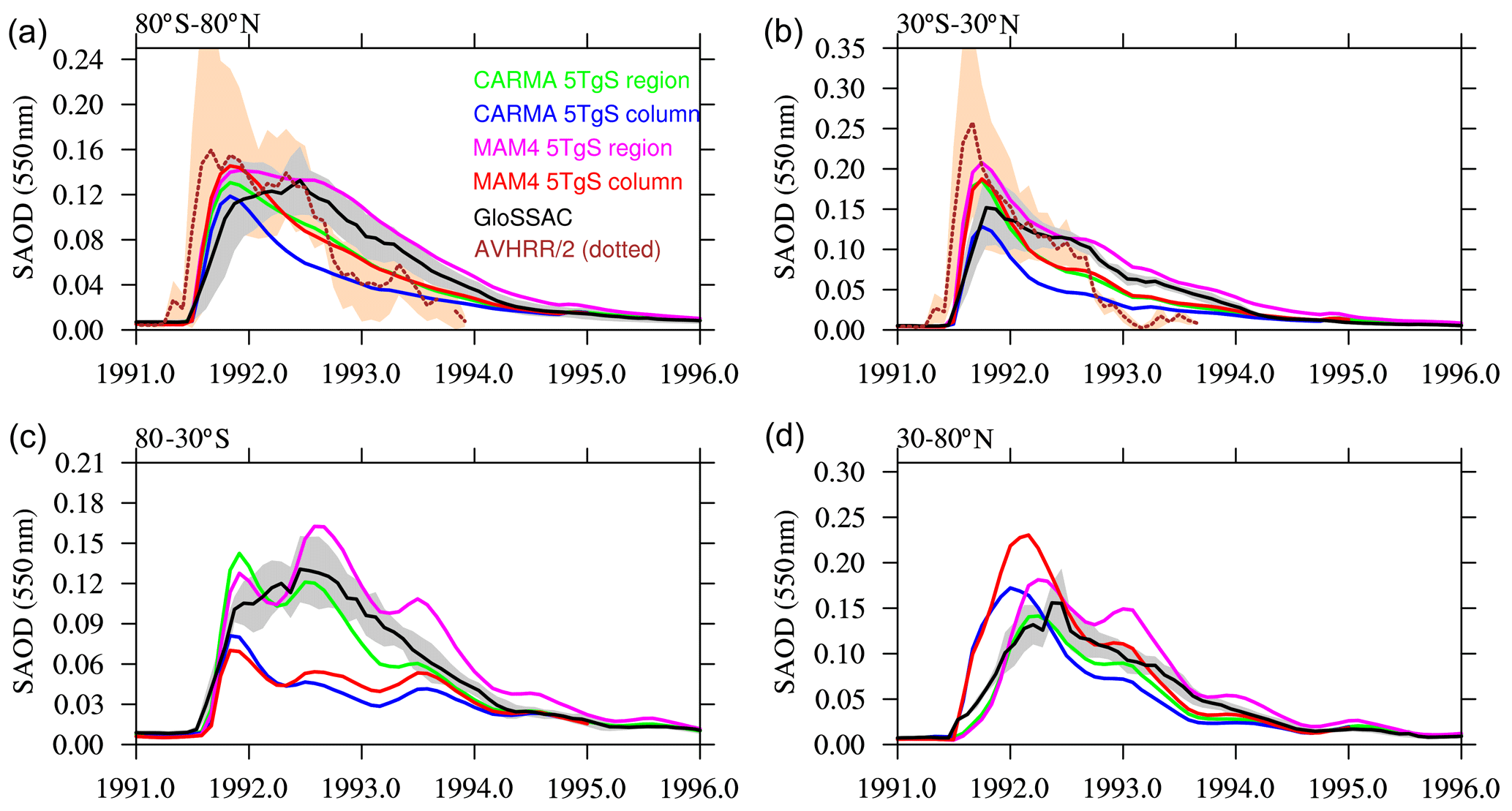
Figure 2Stratospheric aerosol optical depth (SAOD) of different WACCM-MA model experiments using injections in a single column and regional injections using MAM4 and CARMA (see legend) for four different latitudinal averages (different panels) in comparison to GloSSAC and AVHRR/2 data (only available between 70∘ N and 70∘ S and therefore only shown for panels a and b). Gray and tan areas indicate the 2σ standard deviations of the observational datasets for the corresponding region.
Aerosol extinction comparisons between GloSSAC and model simulations with single-column injections averaged between January and March 1992 (Fig. 3b, e) show that single-column injections in both MAM4 and CARMA result in a spread of aerosols primarily towards the high NH latitudes, while observations also show a spread of aerosols in the SH lowermost stratosphere 6–9 months after the eruption. Both MAM4 and CARMA show the largest aerosol extinction in the NH polar region lower stratosphere, which points to the transport of aerosols that is too strong towards the NH high latitudes. Some of the enhancement of aerosol extinction in the SH below 13 km, as shown in observations and models (see Fig. 3), is the result of the eruption at Cerro Hudson, which erupted 15 August 1991, at 45∘ S and 72∘ W and injected 2.6 Tg SO2 into the SH midlatitudes and about 0.75 Tg of SO2 between 12 and 16 km (Carn et al., 2016).
An earlier study by English et al. (2012) showed a much better agreement of aerosol properties after the Mount Pinatubo eruption, using WACCM Version 4 and CARMA. In that study, English et al. (2012) assumed an injection region that covered 14∘ N–2∘ S, 95–115∘ E between 15–28.5 km over 48 h (with a peak at 21 km) and used injections of 10 TgS (double the amount used here and towards the high end of observations). They identified the injection region based on observations of the Total Ozone Mapping Spectrometer on 16 June 1991. Comparisons of this earlier model study with satellite observations showed a good representation of the SAOD (English et al., 2012). However, this model version did not include the coupling between aerosols and radiation, which may have led to shortcomings in the transport of aerosols after the eruption. Based on these considerations, we developed a new injection profile for the Mount Pinatubo eruption that covers a region between 15∘ N–5∘ S, 120∘ E, with an altitude profile between 19–27 km over 9 h (with a peak at 22 km) and an initial extent of 5 and 7 TgS (as discussed below). We use injection altitudes above 19 km to ensure that most of the aerosols were directly emitted into the stratosphere, which allowed for a smaller injection amount than that used by English et al. (2012) and expanded the injection region slightly horizontally to allow more aerosol movement into the SH.
The updated injection details for the Mount Pinatubo eruption result in an improved agreement of extinction and the SAOD with GloSSAC using both MAM4 and CARMA configurations (Figs. 2 and 3). In particular, the updated injection region and timing improved the transport of aerosols toward the SH (Fig. 3; right columns). While WACCM-MA MAM4 captures the peak and decline in the SAOD very well in the tropics, it shows a slight overestimation in both NH and SH when compared to GloSSAC (Fig. 2; magenta lines). WACCM-MA CARMA shows a substantial improvement in the SAOD compared to a single-column injection for both tropics and midlatitudes (Fig. 2; green lines). The SAOD values in the tropics are within the standard deviation of the AVHRR/2 observations and GloSSAC observations for the peak value, and the model agrees within the error bars of the observations in the NH and SH. Additional improvements in WACCM-MA CARMA compared to observations, including changes to the nucleation scheme and injection amount are discussed in Sect. 4.1.2.
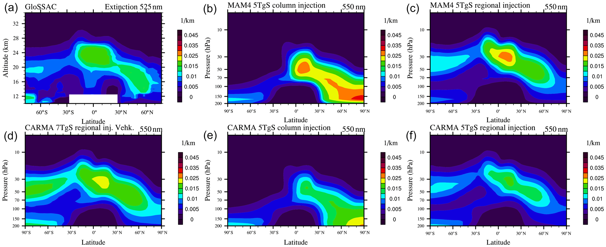
Figure 3Zonal average aerosol extinction (550 nm for the model and 525 nm for GloSSAC), averaged between January–March 1992 for the GloSSAC climatology ((a)) and different model simulations using WACCM-MA.
To analyze the differences between MAM4 and CARMA, we compare the evolution of SO2 and the sulfate aerosol burden and other relevant variables in the volcanic plume within the first 30 and 210 d after the Mount Pinatubo eruption (Fig. 4). The volcanic plume is defined here as locations within the stratosphere (60∘ N–60∘ S and 10–150 hPa) and for grid points that exceed 0.1 µm2 cm−3 surface area density (SAD). We limit the region of interest to air masses within the volcanic plume and exclude the polar region and tropospheric air masses. The main difference between the injection in a single-column and the larger region (as described above) is a much larger limitation of OH in the first month for both MAM4 and CARMA for the single-column injection. This is likely because the SO2 is diluted in the regional case and not able to reduce OH in the same way as the single-column injection case (Fig. 4c).
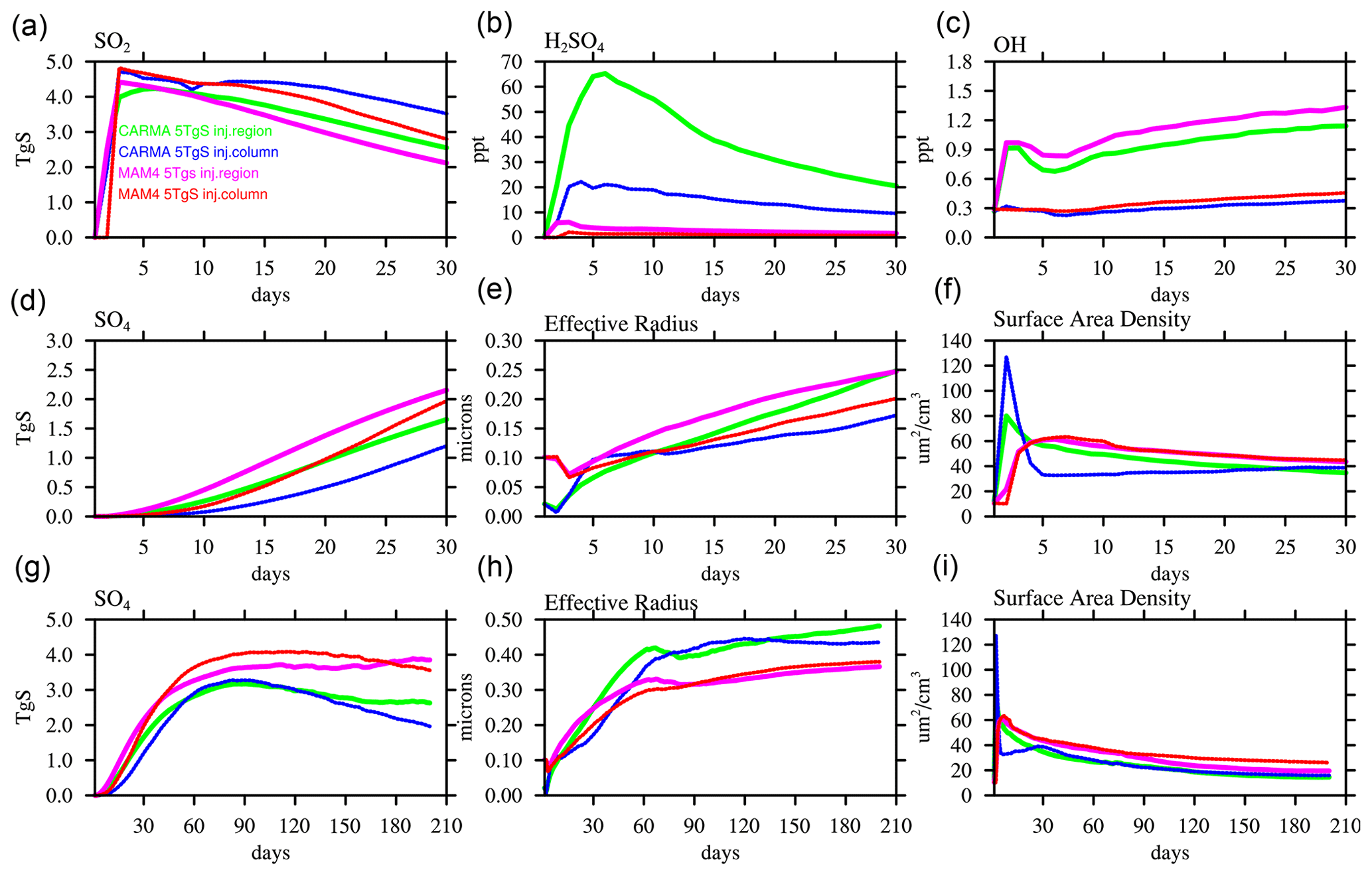
Figure 4Time series of air masses in the volcanic plume between 60∘ N and 60∘ S and between 10 and 150 hPa, as defined by grid points with a stratospheric surface area density larger than 0.1 µm2 cm−3, using the daily averaged model output for different chemistry and aerosol variables over the first 30 d (a–c and d–f) and over the first 6.5 months (g–i) and comparing WACCM-MA experiments with injections in a single grid box (column) and regional injections using CARMA and MAM4.
H2SO4 is formed through the oxidation of SO2 and is therefore dependent on the available OH that is somewhat smaller for CARMA than for MAM4. The nucleation of sulfate from sulfuric acid gas forms small initial sulfuric acid particles (or sulfates) that build up in the smallest pure sulfate bins for CARMA, while the coagulation of similar-sized particles is suppressed due to a low-coagulation kernel. In MAM4, the Aitken mode, which is much larger than the smallest bin in CARMA, serves as a large particle target producing a much larger coagulation kernel with the molecules. Therefore, the acid molecules more rapidly nucleate and further increase coagulation. The initial larger coagulation and growth produce more sulfate in MAM4 than in CARMA. In contrast, in CARMA, H2SO4 builds up in the first 2 d of the eruption and then slowly declines, while sulfate aerosols are nucleating and also condensing on existing particles within the first 30 d in the volcanic plume. Consequently, the effective radius is initially smaller when using CARMA compared to MAM4. The initial very small, effective radius in CARMA, most pronounced for the one-column injection, leads to an initial large peak in the SAD in the first day or two and a later decline below the SAD value in MAM4 after about 5 d. For both aerosol models, injections in one column result in a smaller effective radius and sulfate mass than regional injections in the first 2 months due to the initial OH limitation for the one-column injections (Fig. 4g, h).
Differences between single-column and regional injections and between MAM4 and CARMA are also reflected in the SO2 lifetime (Fig. 5). The single-column injection results in an e-folding time with SO2 of 39 d for MAM4 and 52 d for CARMA, while the regional injection cases show reduced lifetimes of 36 and 45 d, respectively. The longer SO2 oxidation lifetimes delay the production of sulfuric acid gas (H2SO4) in the single-column injection (Fig. 4b). Differences in the lifetimes between MAM4 and CARMA are likely a result of differences in the recycling of SO2 from sulfuric acid (H2SO4) through the photolysis of H2SO4 and SO3, which strongly increases in CARMA in the first day after the volcanic eruption (Fig. 4b).
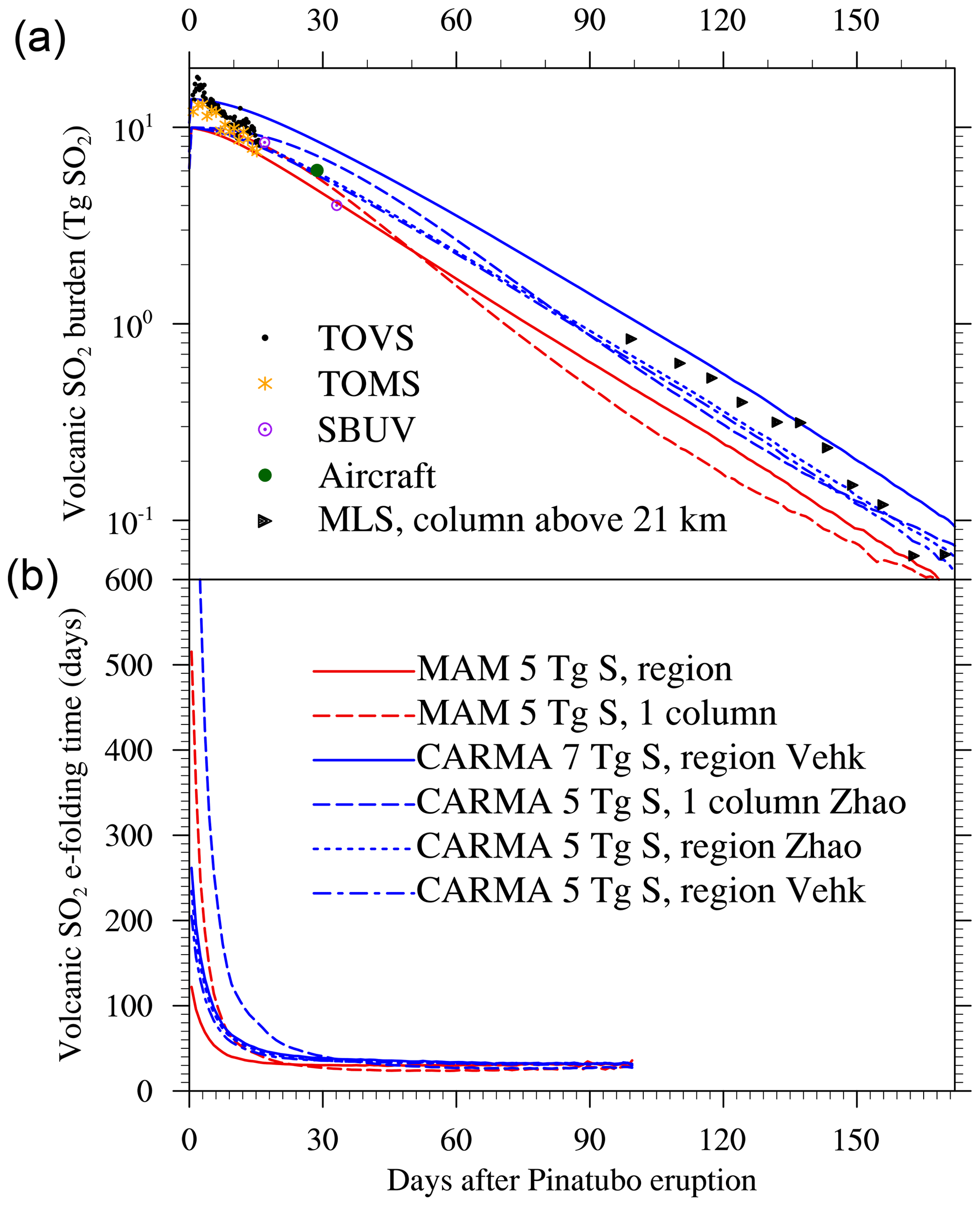
Figure 5(a) The calculated global volcanic SO2 burden following the 15 June 1991 eruption of Mount Pinatubo is compared to observations. The lines show the daily average global burden of SO2 calculated for the WACCM-MA CARMA (blue) and the WACCM-MA MAM4 (red) simulations minus the SO2 burden calculated in corresponding simulations that exclude the Mount Pinatubo eruption. Observations from the TIROS Operational Vertical Sounder (TOVS; black circles) and Total Ozone Mapping Spectrometer (TOMS; orange asterisks) show an initial burden of 13–18 Tg SO2, of which 10 Tg remained after loss to sedimentation ice and ash in the first 7–9 d (Guo et al., 2004). Observations from Solar Backscatter Ultraviolet Radiometer (SBUV), aircraft, and the Microwave Limb Sounder (MLS) are shown, as presented in Read et al. (1993). (b) Volcanic SO2 e-folding time (days) shown as a function of days following the 15 June 1991 eruption of Mount Pinatubo in the simulations. The e-folding time is derived from the daily change in the global volcanic SO2 burden. Volcanic SO2 is calculated by subtracting the global burdens from corresponding simulations that exclude the Mount Pinatubo eruption.
A few weeks after the eruption, the effective radius in CARMA grows larger than in MAM4 and reaches between 0.4 and 0.5µm after 3 months of the eruptions in CARMA, which is in very good agreement with SAGE II observations, as shown in English et al. (2012). The MAM4 effective radius stays below 0.4µm. A better representation of aerosol size in CARMA is expected due to a more comprehensive microphysical scheme using a sectional aerosol model. Furthermore, the SAD in MAM4 is consistently larger than in CARMA, corresponding to the smaller effective radius for a similar or larger mass. The total sulfate mass in CARMA declines slightly faster than for MAM4, which is likely the result of the stronger sedimentation of larger particles and the removal outside the considered region (between 60∘ N and 60∘ S). This is particularly true for the single-injection case, where sulfate aerosols move faster towards the NH high latitudes than the regional injection case (as suggested in Fig. 4b, e, and h).
4.2 Comparisons of different nucleation schemes and Mount Pinatubo injection amount in CARMA
Comparisons in Sect. 4.1. have been performed with the standard nucleation schemes for MAM4 (the Vehkamäki scheme) and CARMA (the Zhao scheme; see Sect. 2.3 for more details). Here we are exploring possible differences between MAM4 and CARMA that may be caused by differences in using the nucleation scheme (Figs. 6 and A1). Using the regional injection profile and injections of 5 TgS, we performed two model simulations using WACCM-MA CARMA, with one using the original nucleation Zhao scheme and a second with the Vehkamäki scheme, which is consistent with what has been used in MAM4. In addition, we also tested simulations that increase the injection amount to 7 TgS using CARMA, which is more in line with an updated observational study by Fisher et al. (2019), who suggested even larger sulfur injections of up to 8 or 9 TgS. However, some of the initial sulfur injection amount is expected to be removed early by reactions with volcanic ash (Zhu et al., 2020), which is not included in this model version.
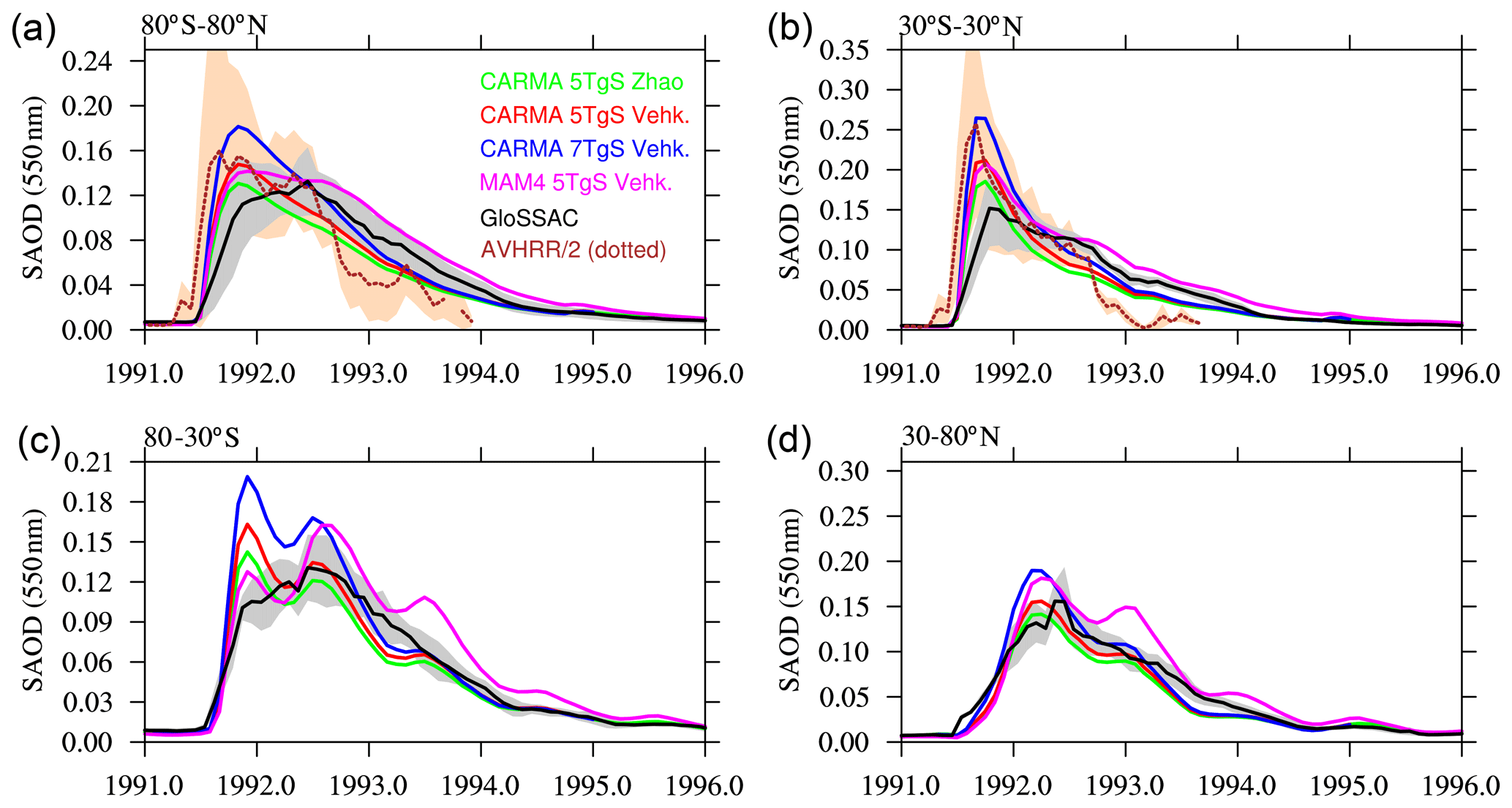
Figure 6Stratospheric aerosol optical depth (SAOD) of different WACCM-MA model experiments with regional injections, using different nucleation schemes and injection amounts for MAM4 and CARMA (see legend), illustrated for four different latitudinal averages (different panels) in comparison to GloSSAC and AVHRR/2 data (only available between 70∘ N and 70∘ S and therefore only shown for a and b). The default nucleation scheme for CARMA is the Zhao scheme (green colors); for MAM4, it is the Vehkamäki scheme (magenta). Using the Vehkamäki scheme in CARMA for different injection amounts is shown in red (5 TgS) and blue (7 TgS). Gray and tan areas indicate the 2σ standard deviations of the observational datasets for the corresponding region.
Using the Vehkamäki scheme with CARMA shows a slight increase in the SAOD compared to using the Zhao scheme (Fig. 6; green and red lines). The additional, larger injection of 7 TgS compared to the 5 TgS (Fig. 6; blue lines) results in a larger SAOD peak in the tropics, which is more in line with what has been observed by AVHRR/2. It is close to or within the range of the GloSSAC standard deviation during the decline in the plume for the different regions. Comparisons of different relevant species in the volcanic plume in the first 30 and 210 d after the eruption (Fig. A1) indicate that the Vehkamäki scheme results initially in slightly larger H2SO4 and does not show the initial peak in the SAD, which points to slightly larger nucleation and faster condensation and slightly reduced recycling of SO2 than the Zhao scheme. Using the Vehkamäki scheme compared to the Zhao scheme does not significantly impact the SO2 lifetime, which is reduced from 45 to 44 d. The more considerable injection extent, using 7 TgS instead of 5 TgS, increases the available sulfur and H2SO4 for condensation, resulting in a similar sulfate burden compared to MAM4 for the first month after the eruption and a much larger burden of the peak after 2–3 months.
4.2.1 Particle number density distribution comparisons between CARMA and MAM4
Based on the above analysis, WACCM-MA with both MAM4 and CARMA is able to reproduce the observed SAOD evolution after the Mount Pinatubo eruption if specific injection regions and amounts are applied. MAM4 needs a 5 TgS injection to agree well with the observations in the tropics, with some overestimation of aerosol optical depth (AOD) in the mid- to high latitudes. CARMA does better with larger injections of SO2 in the range of 7 TgS, which agrees with SO2 observations. However, the effective radius and surface area density are different between the different configurations. In order to evaluate differences in the simulated size distribution between the two models, we compare the model result to the accumulated particle number density distribution from the Laramie, Wyoming, balloon particle counter (Deshler et al., 2003, 2019) at 20 km altitude for two different periods after the Mount Pinatubo eruption in October 1991 and March 1992 (Fig. 7). The accumulated particle number density distribution is a direct measurement. Each column or symbol represents the number density of particles larger than certain sizes. CARMA and MAM4 simulations use the Vehkamäki nucleation scheme and 5 TgS injections for the Mount Pinatubo eruptions (the 7 TgS injection case for CARMA is shown in Fig. A2). For CARMA, pure sulfate and mixed aerosol groups are shown as blue and red histogram plots. We also derive the number size distribution and volume size distribution per radius for both CARMA and MAM4 to identify differences for where the aerosol mass is distributed.
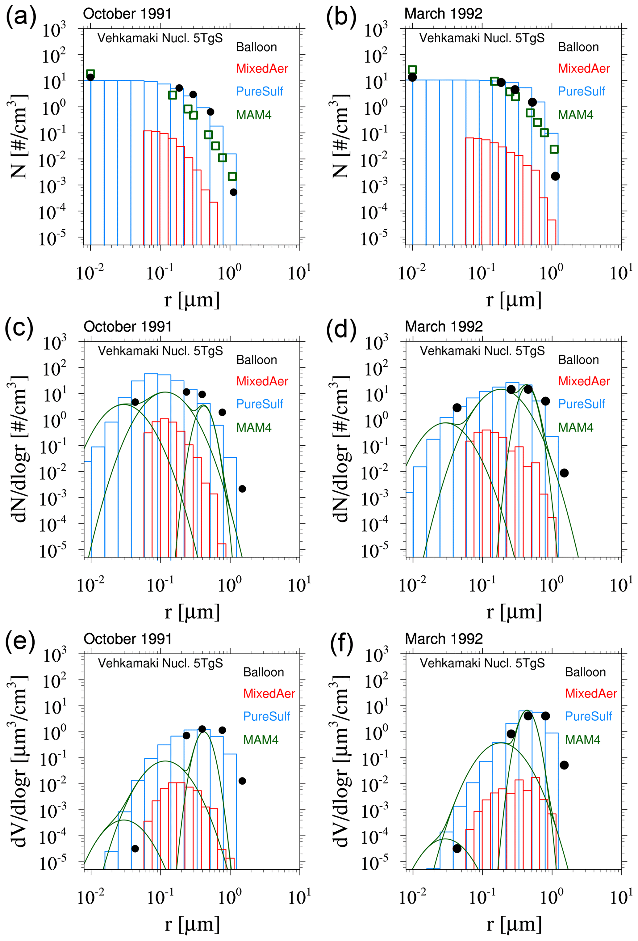
Figure 7Accumulated particle number density size distribution (a, b), number size distribution (ddlogr) (c, d), and volume size distribution (ddlogr) (e, f) comparisons of different model experiments compared to the Laramie, Wyoming, balloon observations (black circles) at 20 km for October 1991 (a, c, e) and March 1992 (b, d, f) after the eruption of Mount Pinatubo. Error bars of the observations are, for the most part, smaller than the illustrated symbol. Monthly averaged model results for different experiments using CARMA and MAM4 with regional injections of 5 TgS (see more details in the text) and the Vehkamäki nucleation scheme. CARMA size distributions are shown in red for the mixed group and in blue for the pure sulfate group. MAM4 particle size modes are shown as green lines.
The CARMA particle number density reproduces the accumulated number distribution compared to observations quite well after 3 and 9 months, following the Mount Pinatubo eruption, except for an overestimation of the accumulated number density for the largest bin around 1 µm for both considered periods. The accumulation of particles in the largest CARMA bin indicates that the selected range for pure sulfates may not be sufficient to reproduce observed aerosol distributions. On the other hand, MAM4 also overestimates the number densities for 1 µm, and the number densities are underestimated between 0.1 and 0.4 µm and overestimated for 0.01 µm compared to the balloon observations. MAM4, therefore, overestimates the total number of smaller particles than observed after Mount Pinatubo, while CARMA shows a better agreement with observations. Number and volume size distributions (Fig. 7c–f) support that MAM4 underestimates the number of accumulation-mode particles and overestimates the Aitken-mode particle number when compared to CARMA. Furthermore, the narrow coarse-mode peak in MAM4 cannot reproduce the observed aerosol sizes near 0.4 µm, where most of the mass is located. This is aligned with a smaller effective radius in MAM4 when compared to CARMA and observations. The smaller particles and larger sulfate burden in MAM4 are also aligned with a larger surface area density (described above) and a larger SAOD in MAM4 than CARMA (consistent with Fig. 4), which can have implications for stratospheric chemistry (not investigated here). Experiments using injections of 7 TgS for simulations with CARMA using the Vehkamäki and the Zhao (not shown) nucleation schemes show very similar size distributions (Fig. A2 for Vehkamäki).
4.3 Stratospheric optical and aerosol properties and total column ozone between 2001–2020
After the large Mount Pinatubo eruption in 1991, we experienced a volcanically quiet period until early 2000. The surface area density and particle number density distribution for the volcanically quiet period of the different experiments are compared to the balloon particle counter in July 2003 at Laramie, Wyoming, at 20 km altitude (Fig. 8). CAMchem and WACCM-MA using CARMA with the Zhao and the Vehkamäki nucleation scheme reproduce the SAD from observations very well. CAMchem and WACCM-MA using MAM4 somewhat overestimate the mean SAD when compared to the observations in CAMchem in particular, which is mostly outside the error range of the observation. The uncertainty in the SAD from the observations is about 40 % (Deshler et al., 2003) because the SAD is a derived measure from the observed size distributions. Comparing the accumulated particle number density distribution allows a more direct comparison between observations and model results (as performed in Fig. 8b–e). CAMchem and WACCM-MA using CARMA agree with the observations for most size bins, with a slight overestimation in the number for the two largest bins, which is more pronounced when using WACCM-MA. For CAMchem, the Zhao nucleation scheme shows a slightly better agreement with observations, which is not the case for WACCM-MA. In contrast, configurations using MAM4 show an overestimation of the aerosol number for sizes larger than 0.4 µm, which is part of the MAM4 coarse mode. Observations also indicate an overestimation in the number densities of the smallest aerosol size, namely the Aitken mode in MAM4, which is more pronounced in CAMchem. The larger number of smaller aerosol particles is likely responsible for the larger SAD shown in Fig. 8b and d. In the following, we only discuss results using the Zhao nucleation scheme for CARMA. As shown later, CARMA with Zhao performs better than using the Vehkamäki nucleation scheme in the troposphere compared to observations.
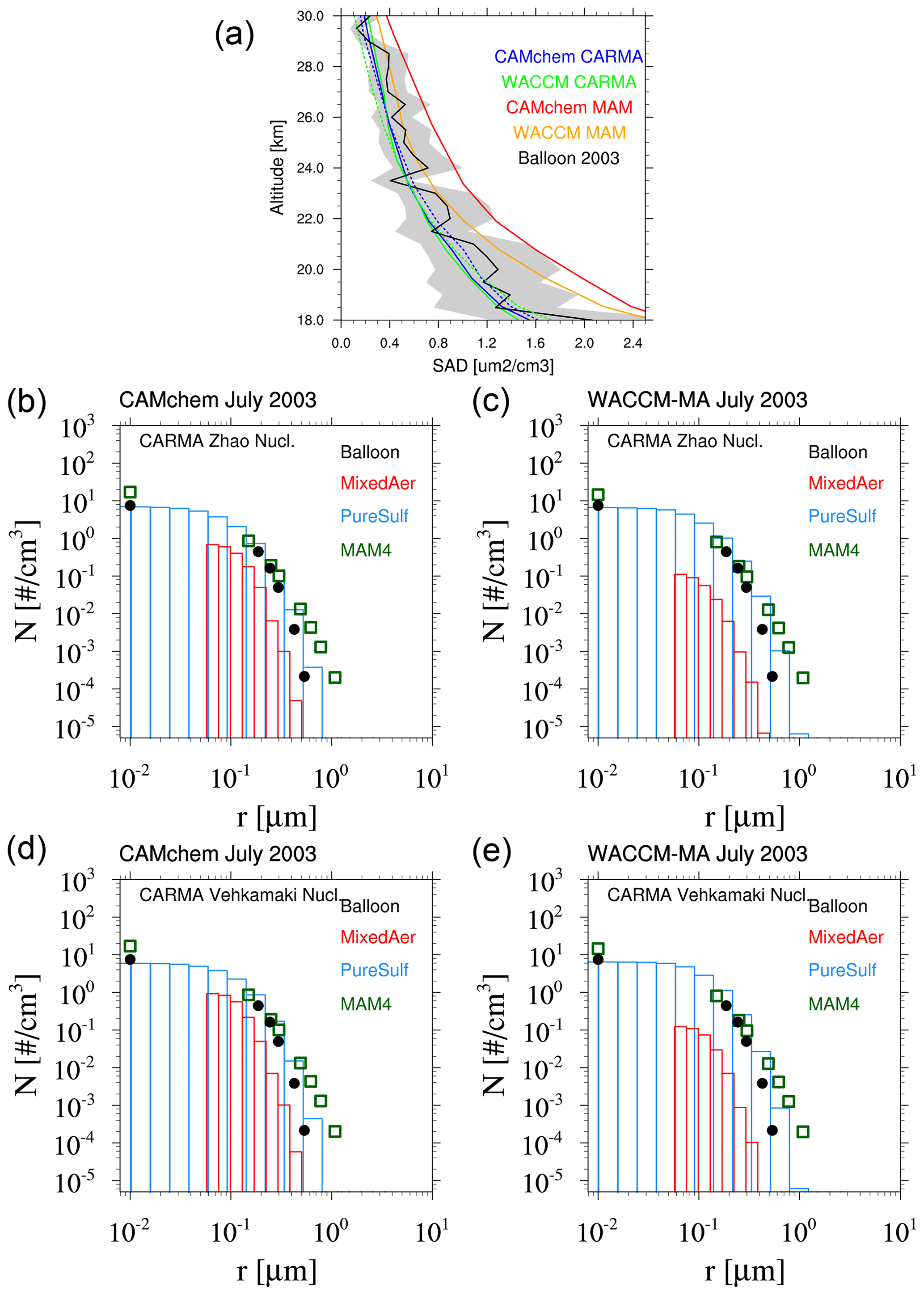
Figure 8Surface area density (a) and accumulated particle number density size distribution comparisons of monthly averaged model results for different experiments (b–e) with CAMchem (b, d) and WACCM-MA (c, e) as compared to Wyoming balloon observations for stratospheric aerosol background conditions at 20 km in July 2003. (a) For CARMA, the results are based on the Zhao (solid lines) and Vehkamäki (dashed lines) nucleation schemes. (b, c) These experiments used the Zhao nucleation scheme for CARMA and the Vehkamäki nucleation scheme for MAM4. (d, e) All experiments used the Vehkamäki nucleation scheme.
After 2000, a series of smaller volcanic eruptions emitted up to 1 TgS each, increasing the SAOD (Santer et al., 2014). WACCM-MA and CAMchem configurations reproduce the global annual mean SAOD evolution within the standard deviation of GloSSAC (Fig. 9). For background conditions, model experiments using MAM4 show a slight underestimation compared to GloSSAC climatological mean, while simulations with CARMA are very close to the observed values. All the experiments show a relative overestimation of the peak values, particularly for the Kasatochi eruption in 2008 and other larger eruptions. The reasons for the overestimation of these volcanic eruptions may be a result of the specifics of the volcanic emission database Neely and Schmidt (2016), or it may be due to SO2 interactions with ash and ice that are mixing in the simulations, which will have to be investigated in future studies.
.
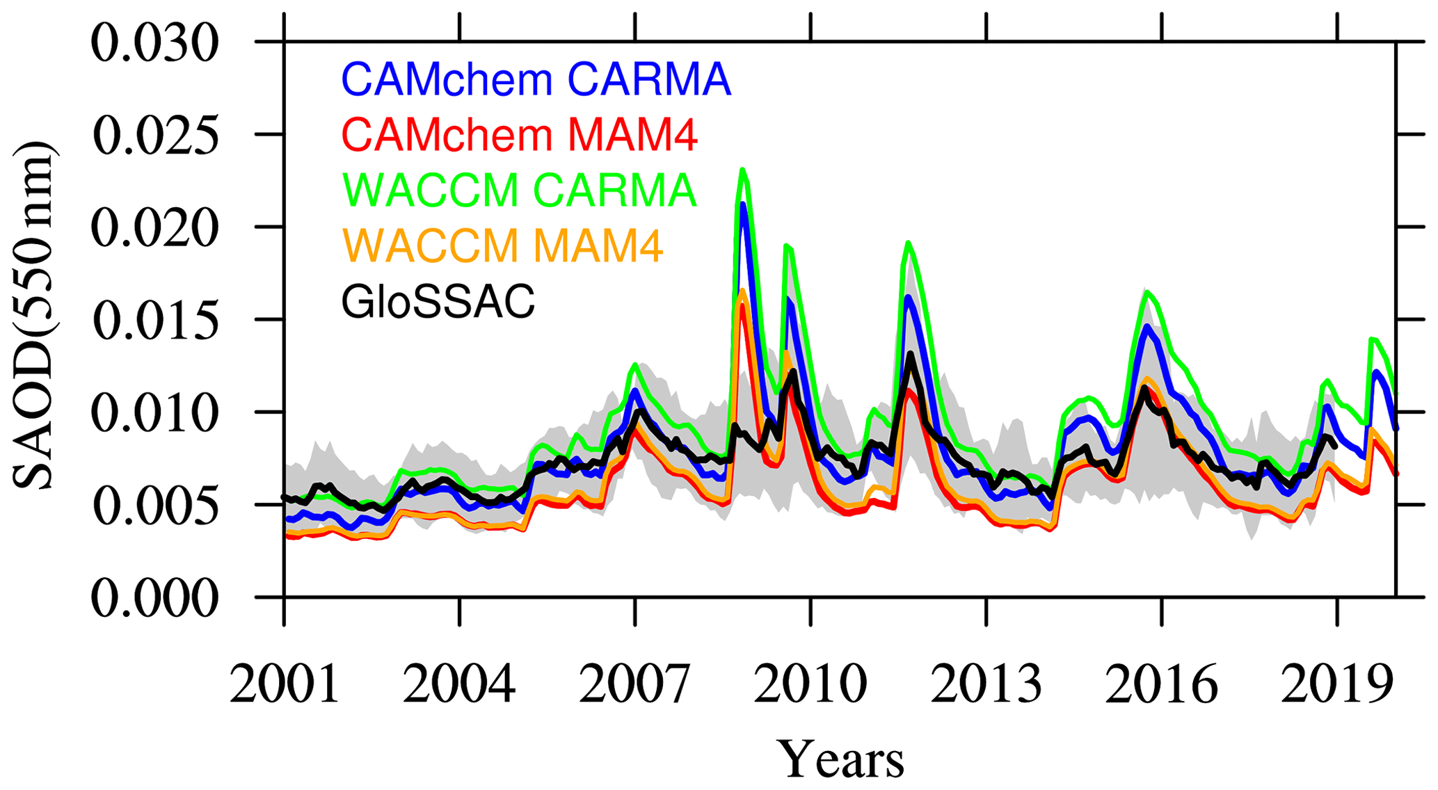
Figure 9Global mean stratospheric AOD (SAOD) comparisons between different model experiments (see the legend) between 2001 and 2020, as compared to GloSSAC. The gray area indicates the 2σ standard deviations of the observational dataset. The CARMA model experiments use the Zhao nucleation scheme, and MAM4 experiments use the Vehkamäki nucleation scheme
In addition to the evaluation of aerosol properties, we also performed a comparison of total column ozone (TCO) in both the stratosphere (Fig. 10) and troposphere (Fig. A3) with the Microwave Limb Sounder (MLS) or Ozone Monitoring Instrument (OMI) climatology between 2004 and 2010. All model configurations generally reproduce the zonal structure and seasonality of observed stratospheric TCO, with fairly good agreement in the tropics and midlatitudes. All the models show an underestimation of stratospheric TCO in the SH mid- and high latitudes and some underestimation in NH mid- to high latitudes in July and October. This behavior has also been identified by Davis et al. (2022) and is likely a result of insufficient ozone transport from the tropics to the high latitudes. CAMchem shows slightly larger TCO values in January and April in the NH high latitudes, indicating stronger transport to the NH for CAMchem. No significant differences can be identified between MAM4 and CARMA.
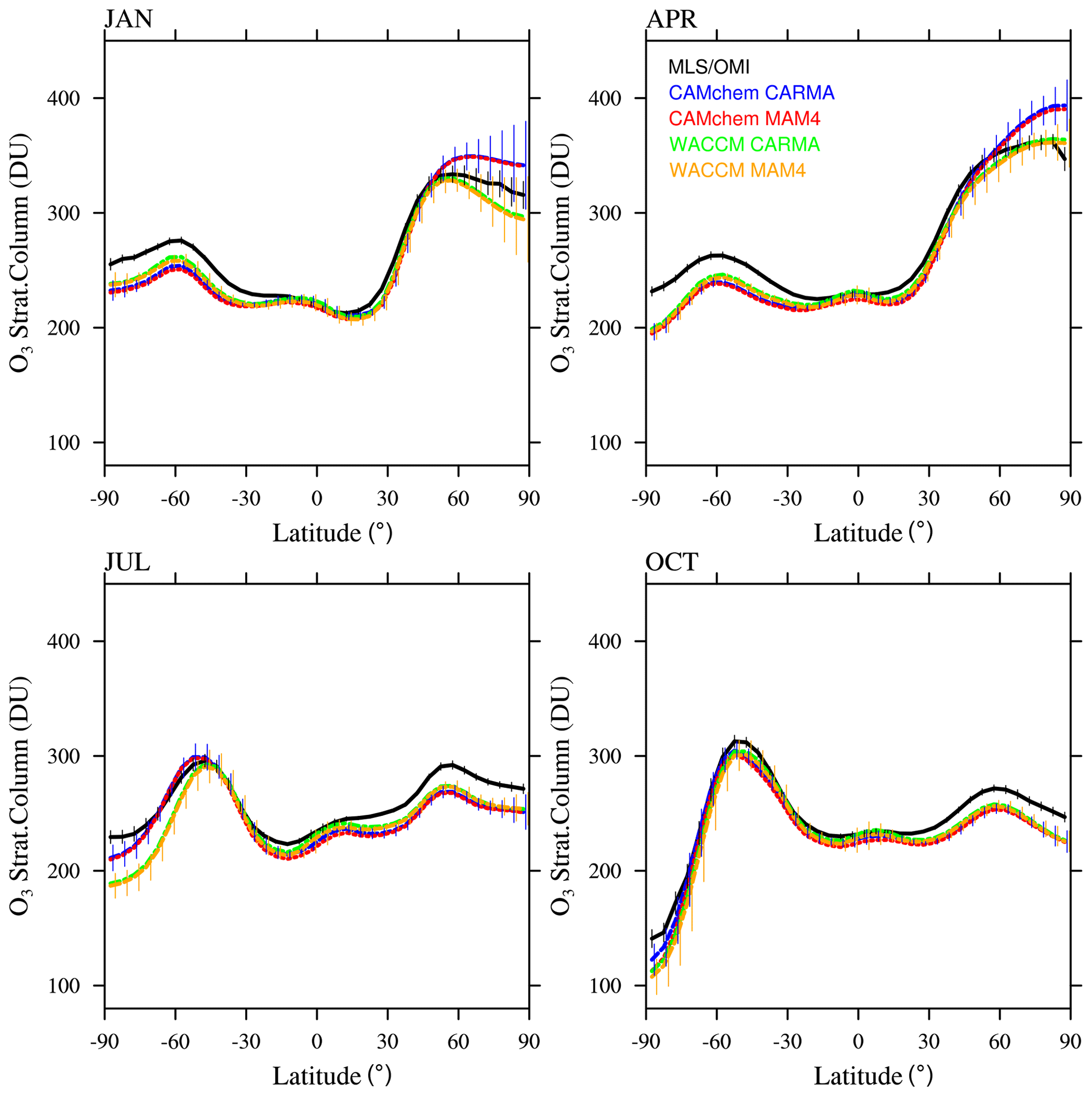
Figure 10Monthly and zonally averaged stratospheric ozone column (in DU) comparison between OMI and MLS observations for 2004–2010 (black) and different model experiments between 2004 and 2010 (for ozone, there is <150 ppb in the model) for 4 months. OMI and MLS error bars (black) show the zonally averaged 2σ 6-year root mean square standard error of the mean at a given grid point, as derived from the gridded product (Ziemke et al., 2011). Model results are interpolated to the same 5∘ latitude grid as the observations, with the error bar showing the standard deviation (1σ) of the interannual variability per latitude interval for CAMchem CARMA and WACCM-MA MAM4.
CAMchem includes interactive aerosols in both the troposphere and stratosphere and, as a low-top model, is more suited for studies focusing on the UTLS and the troposphere. CAMchem simulates oxidants and ozone well (Emmons et al., 2020) and shows a reasonable agreement with tropospheric TCO compared to OMI observations (Fig. A3).
Table 4Averaged total (and tropospheric for sulfate) aerosol burden for 2001–2002 background conditions. All numbers are provided in teragrams for burdens and teragrams per year for the emissions, dry and wet deposition, chemical and aqueous-phase productions, and net gas-to-aerosol exchange. The numbers for sulfate are given in teragrams of sulfur (TgS) for the burden and teragrams of sulfur per year (TgS yr−1) for the other quantities. The lifetime is given in days. Note that trop. is for troposphere.
The following evaluations will focus on CAMchem. However, aerosol burdens and budgets will also be compared with WACCM-MA. We only evaluate the general performance of the model using climatological and background aerosol quantities for the troposphere. A more detailed evaluation of specific case studies will be done in future studies. For this study, we focus on two datasets. The first is the AOD in the visible range (550 nm) from satellite observations from the Moderate Resolution Imaging Spectroradiometer (MODIS) sensors on both the Terra and Aqua platforms, based on the combined Dark Target and Deep Blue AOD algorithms, version 6.1, as documented in Levy et al. (2013). We derived a climatology between 2001 and 2019 for different seasons. We also compare the results to a climatology derived from MERRA-2, a reanalysis product that includes the assimilation of trace gases and aerosols (Randles et al., 2017; Buchard et al., 2017). The second dataset we use is from the NASA Atmospheric Tomography Mission (ATom) aircraft mission (Wofsy, 2018). This dataset is currently the most comprehensive aircraft dataset available, including information on the chemical and aerosol properties. Flights sampled vertical profiles in each of the four seasons (ATom1–4) over a 3-year period between 2016 and 2018. The dataset covers an area from California, moving northward to the western Arctic, then southward to the South Pacific, eastward to the Atlantic, northward to Greenland, and then returning to California across central North America. Based on this dataset, a comprehensive dataset of aerosol properties has been derived (Brock et al., 2021). This dataset of aerosol properties includes information on aerosol microphysical, chemical, and optical properties derived for both dry and ambient conditions from in situ measurements made during the four ATom campaigns. Here, we use the composition-resolved size distributions that range from 3 nm to 50 µm in diameter.
5.1 Tropospheric aerosol optical depth
Both CAMchem CARMA and MAM4 underestimate total AOD compared to MODIS and MERRA-2 in June–July–August (Fig. 11). CARMA underestimates AOD by up to 60 % over the ocean and land and overestimates some land regions over South America and Australia. MAM4 underestimates AOD in the NH up to 80 % and overestimates the SH by more than 100 % in some regions. Significant overestimation of the AOD in MAM4 is shown over land regions in South America, southern Africa, Australia, and parts of northeast Africa and the Middle East. MERRA-2 also overestimates some land regions, including South America and Australia but shows a much better agreement with observations over the ocean. In December–January–February (DJF; Fig. 12), CARMA underestimates the AOD over the ocean, with more negative values in the southern part of the Southern Ocean. As for June–July–August (JJA), some land regions are overestimated, but the values are comparable to MERRA-2, apart from some overestimation over South America. MAM4 over- and underestimates the AOD for different parts of the ocean and does not show the north–south gradient in the AOD differences in December–January–February. The overestimate of the AOD over South America, Africa, and Australia remains for December–January–February.
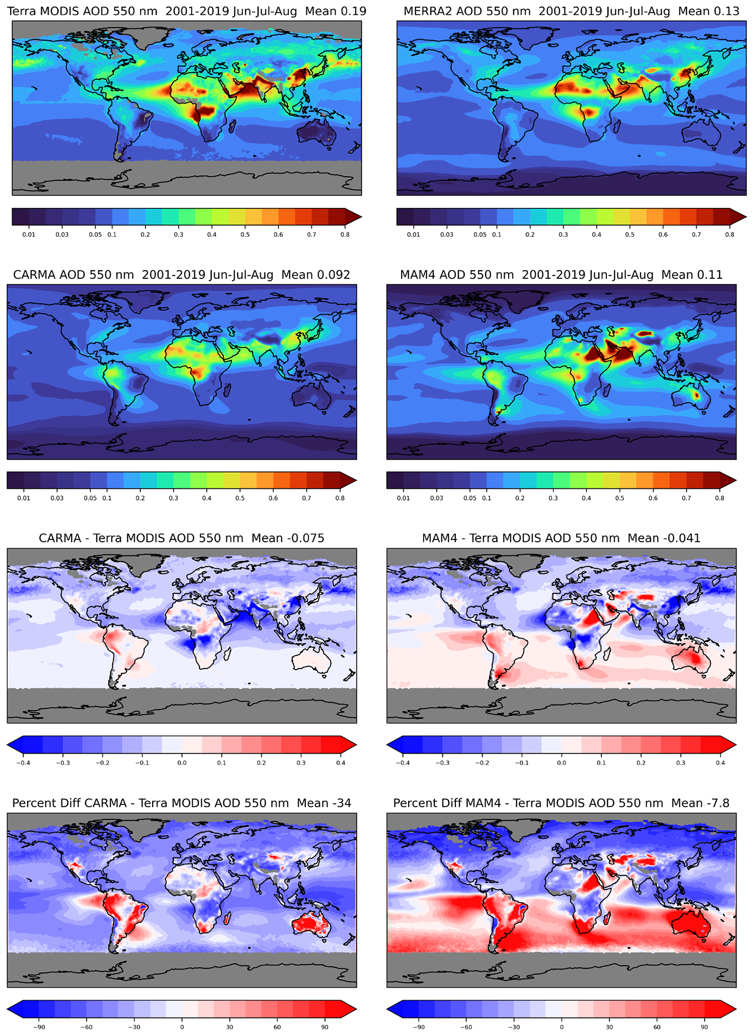
Figure 11Aerosol optical depth in the visible (550 nm) for JJA averaged between 2001 and 2020 from MODIS (TERRA) observations (first row left), MERRA (first row right), CAMchem CARMA (second row left), and CAMchem MAM4 (second row right). The third and fourth rows show the absolute (third row) and relative (fourth row) differences between CAMchem CARMA and the MODIS observations (left) and between CAMchem (MAM4) and observations (right).
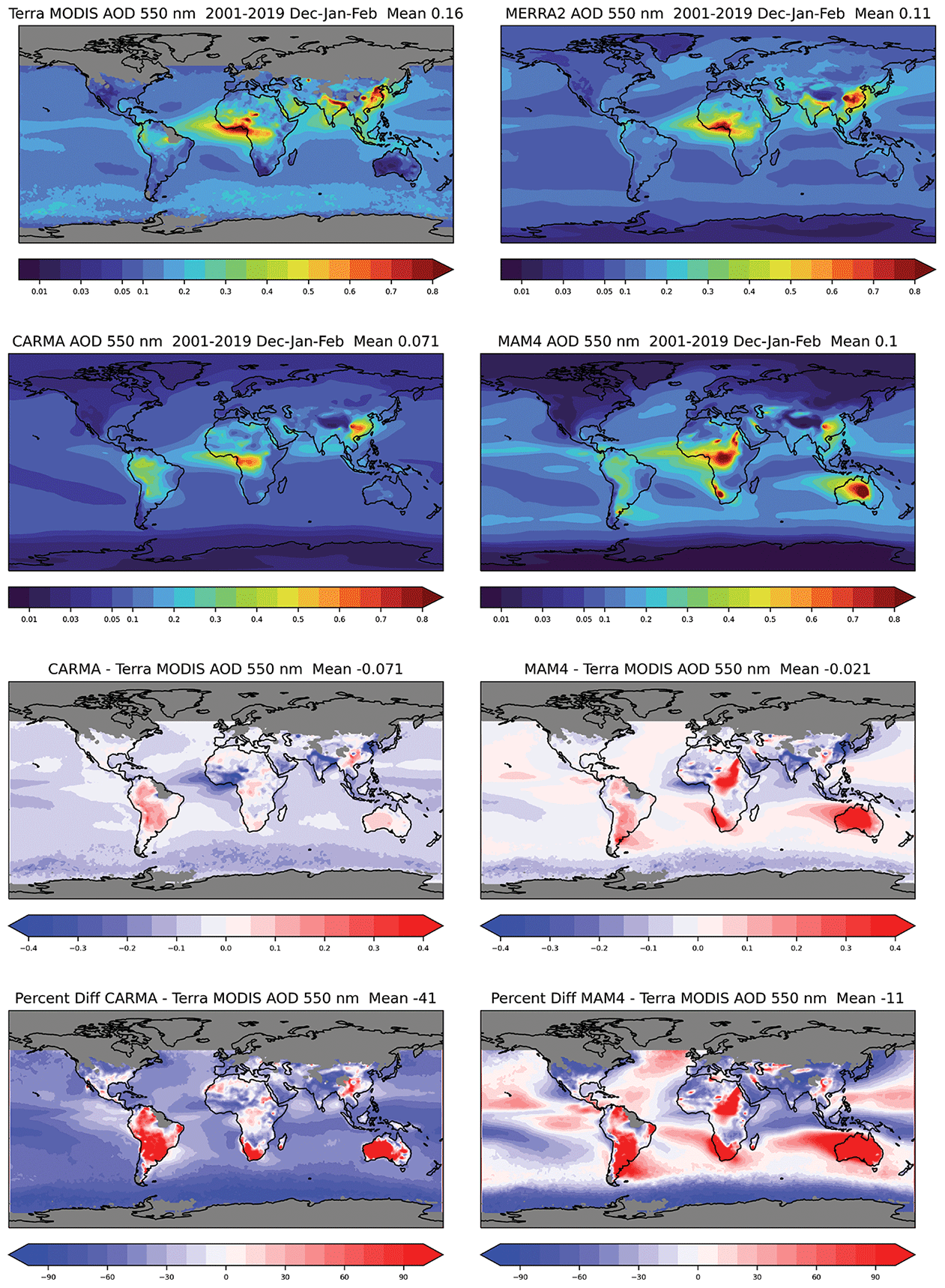
Figure 12As in Fig. 11 but for DJF.
In summary, CARMA shows a stronger underestimation of the global AOD compared to satellite observations and MERRA-2 as a result of a general underestimation of AOD over the oceans due to the missing sources of marine organic aerosols (Yu et al., 2015; Zhao et al., 2021) and missing nitrates in the model (Jo et al., 2021; Lu et al., 2021). The significant overestimation of AOD in the SH in MAM4 is likely a result of too many sea salt emissions. The significant overestimation of AOD over South America for both aerosols models may be a result of a formation of secondary organic aerosols from organic precursor emissions that is too strong. The improved representation of the AOD in CARMA over Africa and also differences over the ocean are likely a result of different sea salt and dust emissions parameterizations in the two configurations (see Sect. 2.4.5). For example, in MAM4, the overestimation of the AOD in the SH in both JJA and DJF, e.g., Australia, South Africa, and Argentina, is due to an overestimation in the dust emissions (Li et al., 2022).
5.2 Comparisons to ATom observations and aerosol budgets
The following section focuses on evaluating the model performance for background aerosol conditions in the troposphere, based on ATom1–4 observations. We use the integrated mass of sulfate, organics, nitrate, sea salt, dust, and black carbon in coarse and fine fractions and extinction provided by the dataset; then we fit lognormal functions to compare them to the different aerosol modes for MAM4 and selected size ranges for CARMA, based on 1 min flight data. We select available data over remote regions over the Pacific (200∘ E to 145∘ E) and Atlantic (0 to 80∘ E) and average over different regions between 60∘ N and 60∘ S. The model interpolated the output to the closest location of the flight track of each 1 min measurement and then averaged it over the same region as the observations. Differences between the model configurations are also discussed based on aerosol budgets, including emissions, deposition, chemical production, and lifetime (Table 4).
5.2.1 Sea salt and dust
Differences in sea salt and dust burdens between CARMA and MAM4 are the result of differences in how emissions are calculated, the microphysical parameterizations that result in different aerosol size distributions, and the resulting differences in the removal processes. In particular, sea salt and dust burdens derived from CARMA are only about half of the amount derived when using MAM4. The 2–3-times-larger emissions in CARMA compared to MAM4 are the result of how emission fluxes are distributed into the bins and modes, with more mass being emitted in the larger size bins in CARMA. On the other hand, coarse-mode emissions in MAM4 are smaller with respect to the total mass than in CARMA, since they are constrained by the narrow standard deviation of 1.2, which was chosen to accommodate the stratospheric coarse model sulfate (Mills et al., 2016; Niemeier et al., 2011). The emissions of larger particles in CARMA also lead to the large deposition of aerosols that have a larger fall velocity than smaller-sized aerosols, as discussed by Yu et al. (2015). On the other hand, MAM4 shows a larger number of coarse model sizes above the boundary layer (1–6 km) for regions with a larger dust and sea salt occurrence (as discussed in Sect. 5.2.4), resulting in relatively more wet removal than CARMA. The larger burden in MAM4 and much smaller dry removal results in a much longer lifetime than in CARMA. While most of the AeroCom model shows similar lifetimes to MAM4 (Adebiyi and Kok, 2020), Lian et al. (2022) have demonstrated that the CARMA aerosol size distributions agree much better with observations, in particular for reproducing larger numbers for larger size bins and a smaller number for the smaller size bins.
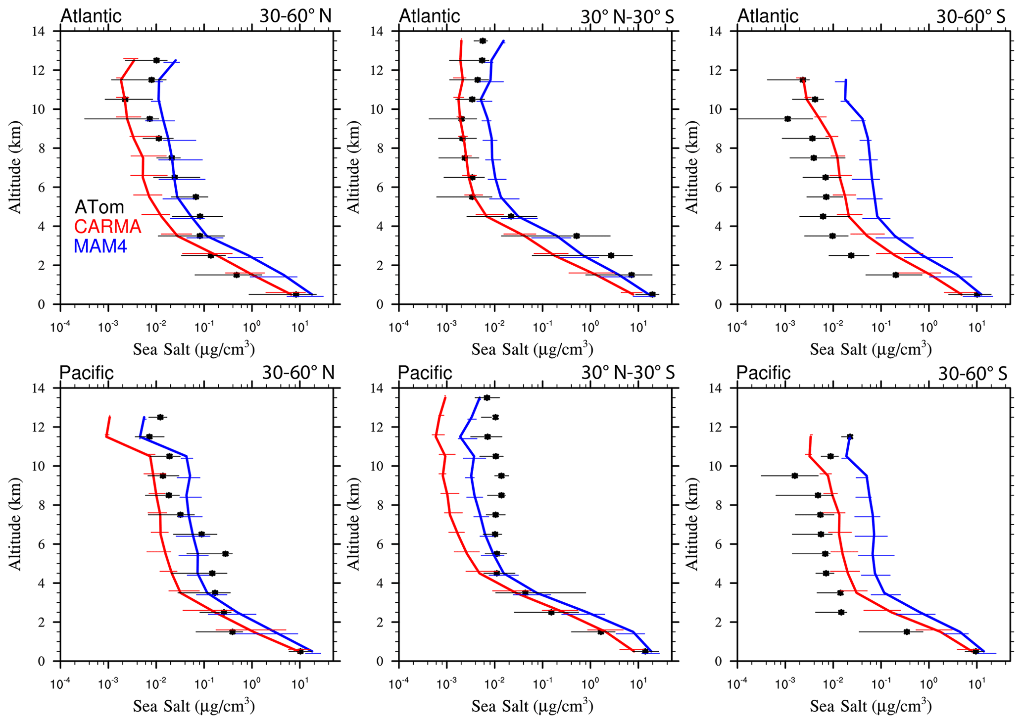
Figure 13Vertical profile comparisons of the median of CAMchem CARMA (red) and CAMchem MAM4 (blue) and ATom1 to ATom4 aircraft observations, averaged over three regions (30–60∘ N, 30∘ N–30∘ S, and 30–60∘ S). The model results were saved on the flight track using the closest location of each 1 min data point and then averaged over the same regions as the observations. Error bars for the observations indicate the 25th and 75th percentile of the distribution for different regions.
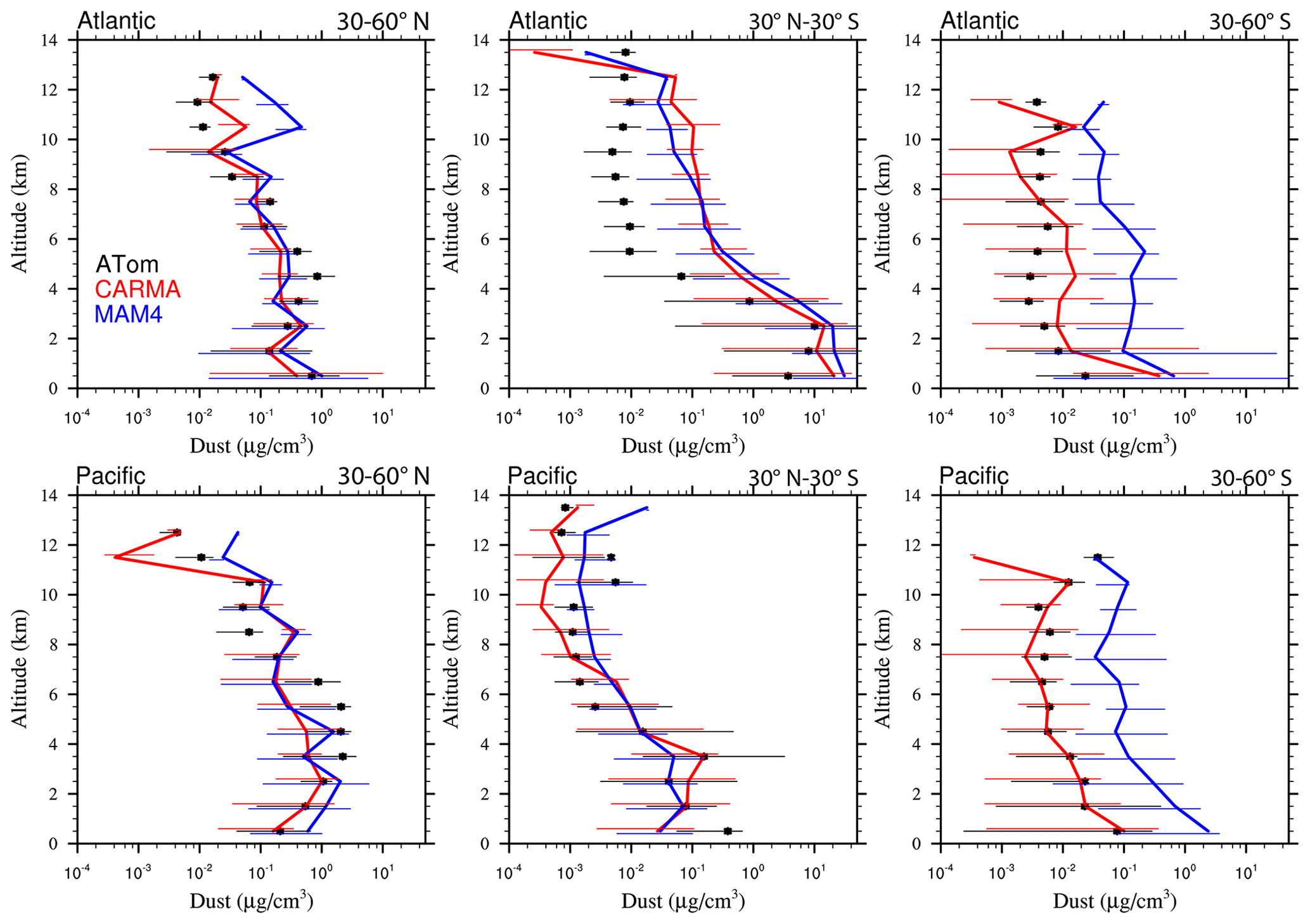
Comparisons to sea salt (Fig. 13) and dust (Fig. 14) with ATom aircraft observations for different regions indicate that both models are within the error bars of the data near the surface for sea salt. CARMA is also within the error bars close to the surface for dust, but MAM4 tends to overestimate dust mass near the surface. The larger AOD over the SH in MAM4 shown in Figs. 11 and 12 is partly a result of the overestimation of sea salt and dust in MAM4 in the midlatitudes of the SH. On the other hand, CARMA underestimates sea salt in the high-latitude NH between 4 and 8 km (Fig. 13). Furthermore, while CARMA shows a very good agreement with the sea salt observations over the tropical Atlantic, it underestimates sea salt in the tropical Pacific above about 4 km. MAM4 overestimates sea salt above 6 km in the tropical Atlantic and in both the Pacific and Atlantic for the SH. Sea salt has strong vertical gradients. It is likely that convection near the measurement sites influences its abundance, and convection is difficult to reproduce in global models both due to its small spatial scale and its episodic nature. More detailed investigations are needed in the future to identify the regional differences that may be caused by differences in clouds and rainfall. CARMA and MAM4 show a constant offset, with CARMA being somewhat lower than MAM4, likely caused by differences in sea salt emissions and the stronger dry deposition in CARMA compared to MAM4.
Both CARMA and MAM4 overestimate dust in the tropical Atlantic region by an order of magnitude in the midtroposphere, while they agree well with observations in the tropical Pacific. This is in contrast to the comparison by Lian et al. (2022), who reported an overestimation over the Pacific and good agreement over the Atlantic, using CESM1 (CARMA) and ATom1 for comparisons. CESM2 using CARMA also reproduces dust concentrations in the Southern Hemisphere midlatitudes well over the Atlantic and Pacific oceans. CARMA and MAM4 also agree very well with the observation for the NH midlatitudes. The main difference between CARMA and MAM4 is an overestimation of dust in MAM4 by 1 order of magnitude in the SH midlatitudes, while CARMA agrees well with the observations. The derived AOD in CARMA over Australia and southern Africa compares better than MAM4 to observations. Differences between CARMA and MAM4 and the observations in the tropical Atlantic midtroposphere may be related to the wet removal parameterization or shortcomings in resolving deep convection in the model.
5.2.2 Black carbon and organic aerosols
Black carbon (BC) and organic aerosol (OA) are strongly impacted by both dry and wet removal. With freshly emitted BC being mostly hydrophobic, aged BC experiences wet removal as part of the mixed aerosol particle in CARMA and MAM4. While emissions and removal for BC and primary organic aerosols are very similar between the different model configurations (Table 4), CARMA results in a smaller burden and lifetime compared to MAM4, due to differences in the removal of aerosol sizes. CAMchem CARMA and MAM4 are generally within the error bars of the ATom observations, except for the tropical Atlantic upper troposphere and the tropical Pacific for MAM4. In general, CARMA is closer to the observations than MAM4, which shows larger values than CARMA (Fig. 15). Since both model configurations are based on the same wet removal scheme (Sect. 2.4.2), differences are likely due to the different microphysical models with a more comprehensive description of the aerosol size distribution in CARMA.
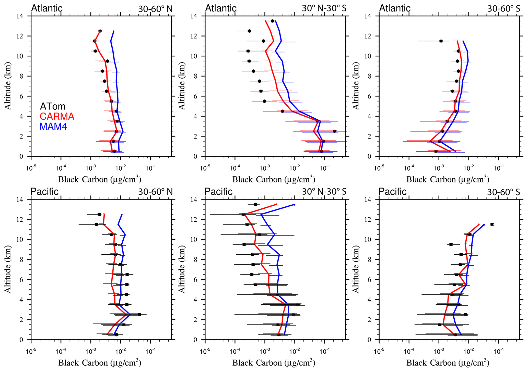
Secondary organic aerosol (SOA) are based on the VBS approach in CAMchem. WACCM-MA uses a more simplified approach that assumes only one volatility bin. Differences in the SOA aerosol production and removal processes between CAMchem and WACCM-MA result in larger production and removal for WACCM-MA CARMA (Table 4). However, the different aerosol schemes, CARMA and MAM4, show fairly similar results in CAMchem in production and removal processes and when compared to ATom observations. In contrast to both microphysical schemes in CAMchem, WACCM-MA MAM4 does not include photolysis in the standard version used here, while the photolysis of the SOA has only been added in WACCM-MA CARMA. In addition, WACCM-MA MAM4 shows a significantly smaller production of SOA through gas-to-aerosol exchange and a much smaller total burden. A comparison of CAMchem between MAM4 and CARMA and ATom observations (Fig. 16) shows an underestimation of OA at the surface and lower troposphere. A better agreement with the observations occurs in the tropical midtroposphere and SH midlatitudes. The significant underestimation of OA, especially in the NH mid- to high latitudes, is likely a result of the underestimation of SOA aerosol precursor emissions, including anthropogenic sources and biomass burning, which is independent of the aerosol scheme, since both aerosol models show the same bias.
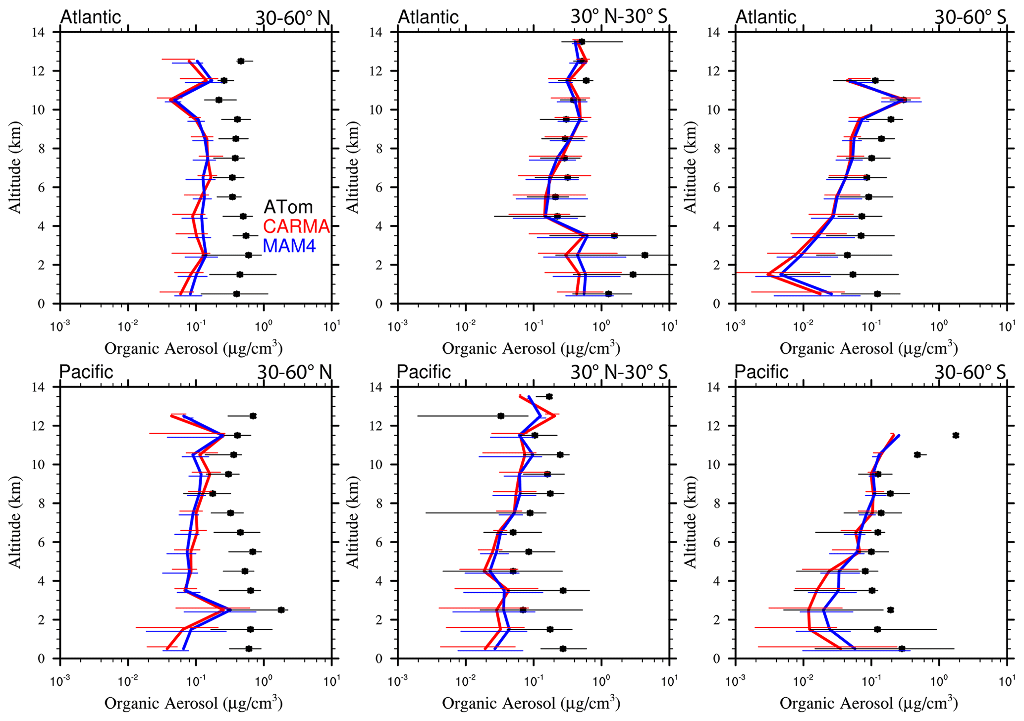
5.2.3 Sulfate aerosol and extinction
The tropospheric sulfate burden in CARMA is 20 % larger for WACCM-MA and close to 40 % larger for CAMchem compared to MAM4. This is much closer than the earlier reported differences of a factor of 2.8 between CESM1 (CARMA) and MAM4 (Yu et al., 2015; Table 4). The production of sulfate by aqueous-phase SO2 oxidation and the production from H2SO4 is slightly smaller in CARMA compared to MAM4, with larger values for CAMchem than WACCM-MA due to the more comprehensive chemistry and larger tropospheric ozone values in CAMchem. The chemical production of sulfate from H2SO4 is of a similar magnitude and very similar among the different model configurations, with slightly larger values for CARMA compared to MAM4, leading to somewhat larger total production using MAM4 than CARMA (Table 4). As with the production, wet and dry removal is slightly smaller in CARMA than in MAM4. The stratospheric aerosol burden (the differences between the total and the tropospheric burden) is larger in MAM4 when using CAMchem and similar to CARMA for WACCM-MA. Differences in burden can result from the details of the aerosol microphysical description (using bins vs. modes), which results in differences in the aerosol size distribution and burden, due to differences in dry and wet deposition. This can also lead to differences in the stratospheric AOD (as discussed above).
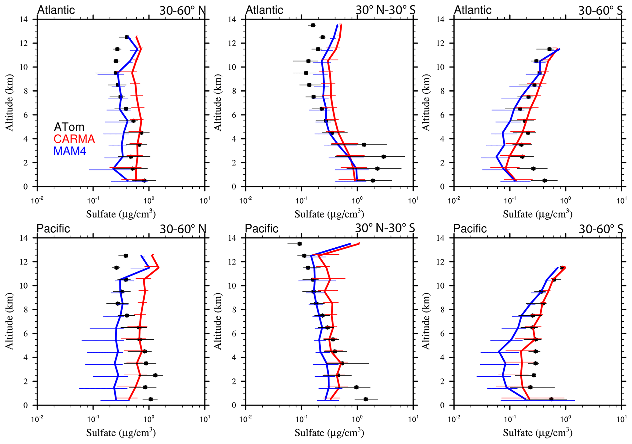
Comparisons to ATom aircraft observations show very similar values for CAMchem CARMA and MAM4 at the surface, with MAM4 showing overall smaller values than CARMA throughout the altitude range, which is consistent with the smaller tropospheric aerosol burden in MAM4 (Fig. 17). MAM4 tends to underestimate sulfates in the lower troposphere, while CARMA tends to overestimate sulfates in the midtroposphere. Both models underestimate sulfate in the boundary layer in the SH midlatitudes and other regions over the Pacific. A possible way to increase sulfates in this region is to consider that marine organics and sulfates are mixed with sea salt, as done in Yu et al. (2015), who assigned a fraction of sea salt flux to sulfate and marine organics.
The combined effect of aerosols on the AOD can be identified by comparing aerosol extinction between the different configurations (Fig. 18). MAM4 is within the error bars of the observations for most regions, except the tropical troposphere above 6 km over the Atlantic. CARMA reproduces the lower troposphere very well, while it shows an overestimation above about 6 km for most regions. This good agreement in CARMA at the surface is likely due to the fairly good representation of sea salt and dust. The overestimation in the free troposphere in CARMA may be the result of an overestimation of sulfates in this region and differences in the size distribution. However, ATom observations are still a snapshot in time, and there are strong vertical gradients in extinction. Global models cannot locate convection well, which may contribute to the difficulty in matching local data on extinction.
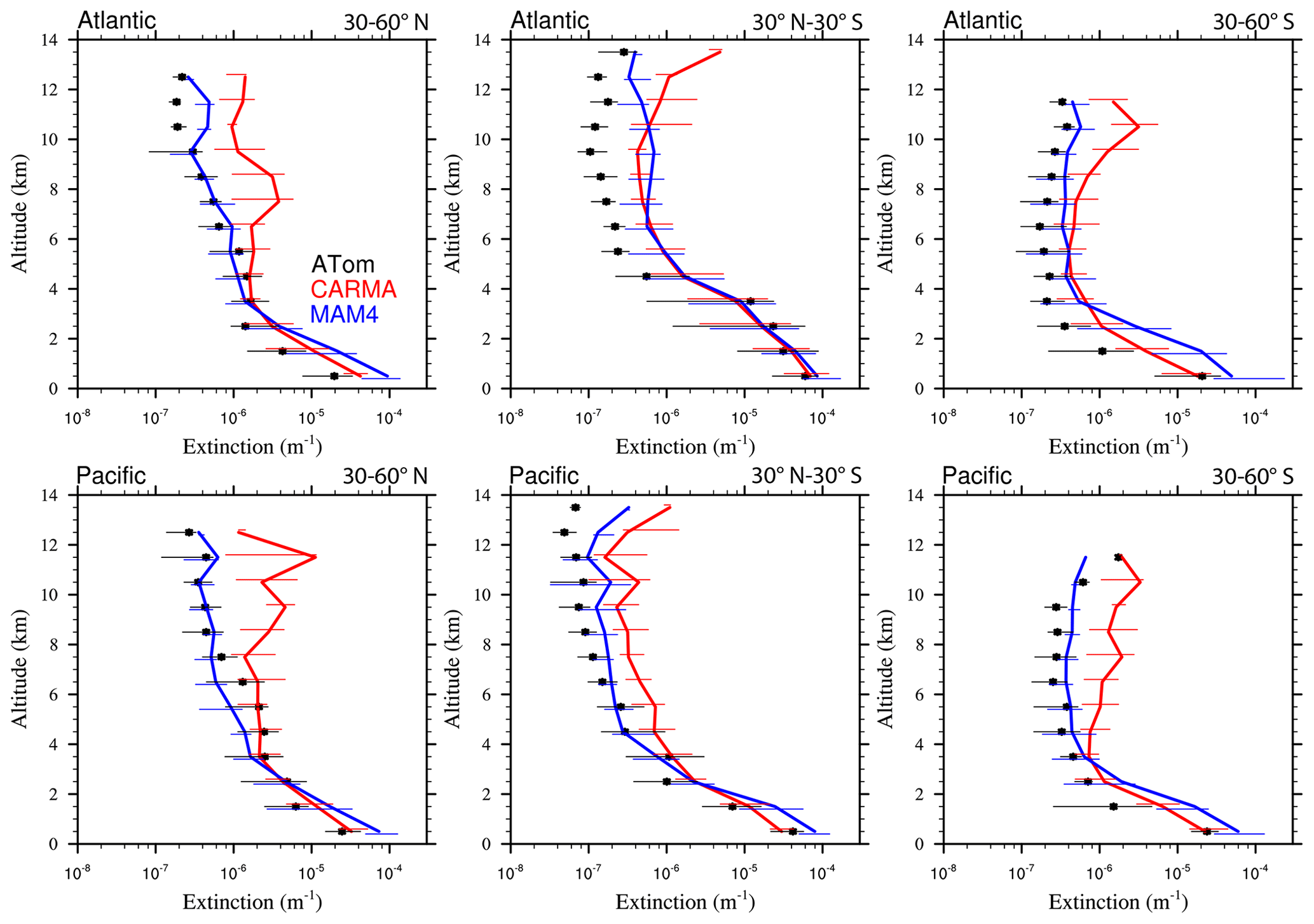
5.2.4 Aerosol size distributions
Number density distributions have been derived for distinct bins using observations from all four ATom campaigns (Brock et al., 2021). These are compared to the CARMA and MAM4 number density distribution over the Atlantic (Fig. 19). The numbers of each of the different bins have been averaged for a large region (0–30∘ N, 0–30∘ S, and 30–60∘ N) and for altitudes between 1–6 km (top row) and 6–12 km (bottom row; left and middle). We also compare stratospheric values, which are defined for all observations that show ozone >150 ppb, in the bottom right of Fig. 19. CARMA size distributions are shown for pure sulfates (blue) and mixed aerosols (red) separately. Since these two CARMA aerosol groups cover different size ranges and sizes, we are not combining them here. The larger of the two groups in the logarithmic representation in Fig. 19 can be viewed as the dominant group, which is comparable to the total number shown in the observations.
For the tropics in the lower troposphere averaged between 1–6 km (Fig. 19; left top panel), both CARMA and MAM4 represent the shape of the accumulation-mode aerosol distribution observed during ATom. The models also represent the second peak in the distribution between 1 and 6 µm for the tropical NH Atlantic, which is expected to be a result of the contribution of dust from West Africa. Observations show very similar values for the larger sizes. While the MAM4 accumulation model also reproduces the shape of the ATom size distribution well and reproduces some of the larger sizes above 1 µm, the fairly narrow peak of the coarse mode cannot reproduce the largest sizes. There is also a gap between the Aitken and coarse mode at around 1 µm that is not covering aerosols in that range. Furthermore, CARMA slightly underestimates Aitken-mode numbers, while MAM4 does not capture nucleation-mode sizes below 0.003 µm.
For 30–60∘ N over the Atlantic (similar to values over the Pacific and in the SH), the number of the mixed aerosols in CARMA is significantly higher than observed, with some overestimation also seen in MAM4. The mixed aerosol group in this CARMA setup is restricted to sizes from 0.05–8.7 µm. However, the lowest bin size is still too large to represent, for example, the nucleation of SOA. This results in an accumulation of newly formed SOA particles in the smallest mixed group bin, which is likely to lead to larger numbers than observed, particularly in the tropical midtroposphere and polluted areas. The mixed group bin structure in this model had been adopted from Yu et al. (2015). This comparison reveals the need for mixed groups that cover smaller aerosol sizes than in our model configuration. Still, the number of bins is an adjustable parameter and can be changed in the future. The pure sulfate aerosol group in CARMA covers much smaller bins than the mixed aerosol group and shows an underestimation for aerosols between 0.005–0.1 µm in particle radius compared to the observations. The lack of smaller-sized bins in the mixed aerosols is a likely reason for not representing these sizes correctly, as discussed above. The MAM4 Aitken mode reproduces the number size distribution for sizes around 0.01 µm for the lower troposphere but overestimates numbers between 6–12 km.
The shape and magnitude of the number distribution of aerosols in the lower stratosphere (over the Atlantic and Pacific) are represented well in CARMA compared to the ATom observations (Fig. 19; bottom right panel). The model shows a slight underestimation between 0.01 and 0.1 µm. While there may be a lack of SOA in these size ranges, the underestimation may also result from missing meteoric dust and nitrates in the model (Murphy et al., 2021). MAM4 overestimates Aitken- and coarse-mode numbers, which is in agreement with what was shown in Fig. 8, compared to the Wyoming balloon observations.
Number density distributions in comparison to ATom observations are also derived for CAMchem CARMA using the Vehkamäki nucleation scheme (Fig. A6). For the lower troposphere, pure sulfates show a significant underestimation in number, whereas the Zhao scheme produces values that are much closer to the observations. On the other hand, for the upper troposphere and lower stratosphere, the Vehkamäki nucleation scheme does produce a reduced overestimate in the number of the very small bins of the pure aerosols group, which is also the case for the Zhao scheme. However, the values of the sizes that included most of the mass (larger 0.01 µm) are still largely underestimated. We conclude that the Zhao nucleation scheme is more suited for reproducing aerosol distributions in the troposphere and lower stratosphere compared to the Vehkamäki nucleation scheme.
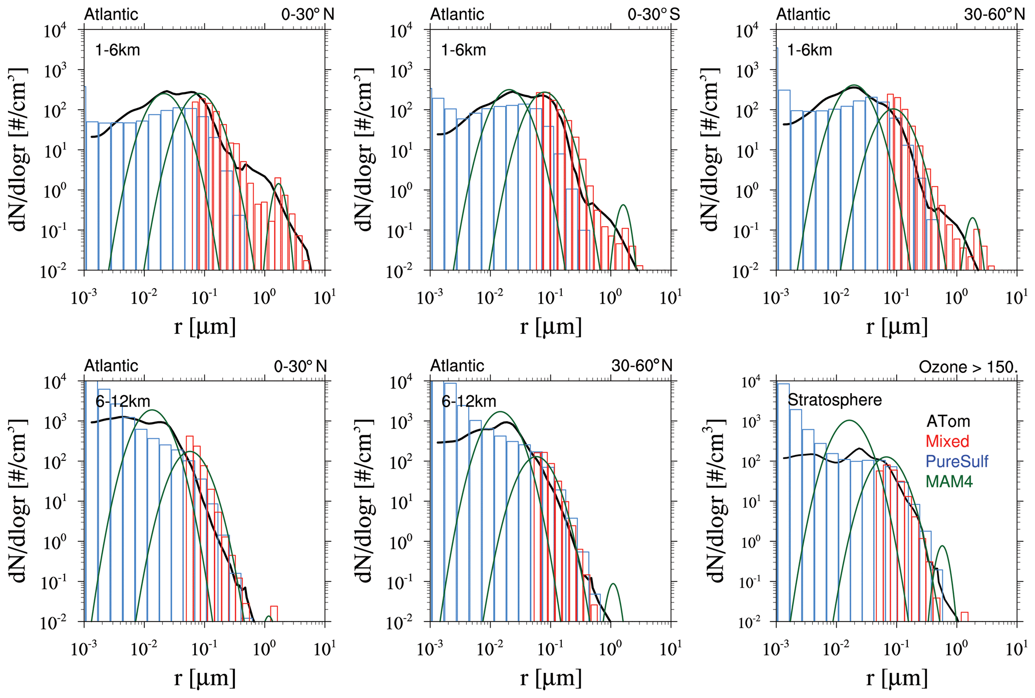
Figure 19Number density distributions of CAMchem CARMA results for size bins of the mixed aerosol (red) and pure sulfate (blue) group and CAMchem MAM4 modes (green lines) for ATom1 to ATom4 number size distributions from aircraft observations (black). These distributions are averaged over three regions (0–30∘ N, 0–30∘ S, and 30–60∘ N) and over 1–6 km altitude (top row), 6–12 km (bottom left and middle panels), and for stratospheric air masses with ozone mixing ratios >150 ppb (bottom right). The model results were saved on the flight track using the closest location of each 1 min data point and then averaged over the same regions as the observations.
Comparisons between MAM4 and CARMA to ATom numbers in different modes are shown in Figs. A7–A9, based on derived information from the ATom aerosol dataset for the Aitken, accumulation, and coarse modes and compared directly to MAM4. For CARMA, we derive numbers based on the same size ranges used for the data. These comparisons confirm earlier findings that CARMA underestimates Aitken-mode aerosols, likely due to the setup of the mixed aerosol group, while MAM4 is generally within the error bars of the observations. On the other hand, both CARMA and MAM4 are generally within the error bars for the number in the accumulation and coarse mode according to ATom observations, in particular for the tropics. However, comparisons of mode averages do not reveal shortcomings in the size distributions, as discussed above.
The performance of both microphysical models, CARMA and MAM4, has been tested in two different CESM2 configurations nudged to meteorological reanalyses, using the CESM2 CAMchem model with a low top at 42 km and a horizontal resolution of 0.9∘ × 1.25∘, with comprehensive tropospheric and stratospheric chemistry, and the CESM2 WACCM-MA version with a model top at 140 km and a horizontal resolution of 1.9∘ × 2.5∘, with middle atmosphere chemistry. To evaluate the evolution of aerosols and aerosol properties after the Mount Pinatubo eruption (the largest volcanic eruption in the last 25 years), we performed different sensitivity simulations between 1990 and 1995 with WACCM-MA, using both CARMA and MAM4. We also evaluated tropospheric aerosol properties between 2000 and 2020 and between 2016 and 2018 in comparison with observations from the ATom aircraft campaign.
Sensitivity simulations with WACCM-MA compared to the GloSSAC SAOD climatology reveal the importance of applying sulfur injections over a larger region for simulating the Mount Pinatubo eruption when using a global model to be able to reproduce the observed evolution of aerosols. Injections in a single column on a grid cell in horizontal dimension do not result in the observed spread of aerosols into both hemispheres after a few months of the eruption. The coarse model resolution of the global model cannot reproduce the details of the specific meteorological situation during the time of the eruption and cannot reproduce fine-scale dynamics. A regional injection better reproduces the initial spread and improves the aerosol movement later, compared to observations. Furthermore, while the chemistry and physics in WACCM-MA are the same in MAM4 and CARMA, results from different aerosol models show significant differences in the initial aerosol formation (size, surface area density, and composition). The reasons for these differences lie mostly in the details of the parameterization of the size distribution of aerosols. The modal approach in MAM4 (which does not separate nucleation and Aitken modes) shows a much faster formation and growth of sulfate aerosols after the eruption compared to the sectional model approach using CARMA, where nucleated particles first accumulate in a much smaller size bin than the MAM4 Aitken mode, thus restricting coagulation and initial growth.
However, after a few months, aerosol particles in CARMA grow larger than in MAM4. Comparisons with balloon observations indicate a more reasonable representation of the aerosol size distribution following the Mount Pinatubo eruption in CARMA than in MAM4. CARMA and MAM4 both overestimate the number of the large 1 µm particles. CARMA agrees with the accumulated number from the direct measurements for the smaller size bins, while MAM4 underestimates the number between 0.03 and 0.4 µm and overestimates the Aitken model number. Comparisons of the volume size distribution between CARMA and MAM4 reveal that most of the mass after a few months is in the bins that describe the coarse mode, which is well represented in CARMA. However, in MAM4, the coarse-mode distribution is narrower than the corresponding size distribution in CARMA and the observations. The smaller coarse-mode mass and larger accumulation-mode mass in MAM4 are aligned with the smaller effective radius, thus resulting in less aerosol removal and, therefore, more total mass in MAM4 after the Mount Pinatubo eruption. Furthermore, some overestimation of the large 1 µm particles in the largest pure sulfate group in CARMA indicates that the chosen range of the pure sulfates may not cover large enough bins to allow the aerosols to grow larger and instead traps the particles in the largest bin. This limitation may have implications for representing large injections; for example, if climate intervention in the form of stratospheric aerosol injection is applied, then implementing larger-sized bins should be considered in this case.
While the results of each of the models can, to some degree, be adjusted, depending on the injection amount and region, this comparison reveals large uncertainties in our ability to simulate the initial formation of aerosols in a volcanic plume. In addition to the resolution issue, other processes are still not included in either model. For example, the injection of volcanic ash, which is expected to result in a faster formation and removal of injection sulfur by heterogeneous reactions on rock surfaces, has not been included in the current model (Zhu et al., 2020). Furthermore, the lack of observations during the initial volcanic eruption makes it harder to estimate the exact injection amount of gases and aerosols. The current uncertainty can have implications for simulating the effects of stratospheric aerosol injections. Some differences between MAM4 and CARMA are the result of using two different nucleation schemes (the Zhao scheme in CARMA and the Vehkamäki scheme in MAM4). Applying the Vehkamäki nucleation scheme in CARMA increases the initial nucleation rate after the Mount Pinatubo eruption and results in a buildup of more mass in the stratosphere. However, comparisons of the Vehkamäki nucleation scheme for the troposphere reveals reduced performance, and we recommend using the Zhao scheme for applications in the troposphere and UTLS.
Considering the background stratospheric aerosol optical depth (SAOD) and changes in the smaller eruptions after the year 2000, both WACCM-MA and CAMchem using CARMA and MAM4 reproduce the observations within the error bars, with some overestimation of the SAOD for small eruptions. CARMA agrees with the stratospheric number density size distribution from balloon observations, while MAM4 overestimates the number of aerosols in large and small sizes. Comparisons to the AOD from the MODIS satellite data reveal regional differences in the tropospheric aerosol representation in MAM4 and CARMA. In general, MAM4 overestimates several regions that are in particular impacted by dust and sea salt emissions and in particular shows a significant overestimation of AOD in the SH and an underestimation in the NH for JJA. CARMA more generally underestimates the AOD over the ocean. Differences in the emissions and dry removal processes of dust and sea salt are obvious when comparing the global burdens of the different model configurations. Future work needs to include aligning these different approaches to improve comparisons and test the inclusion of marine organic aerosols (e.g., Zhao et al., 2021). CARMA more comprehensively represents larger bins than MAM4 compared to observations, leading to different removal rates in the two aerosol models.
A comparison to ATom aircraft observations over the remote regions over the Atlantic and Pacific shows that both aerosol schemes are generally within the error bars when using CAMchem. CARMA shows a better representation of black carbon than MAM4. However, both aerosol models overestimate BC over the Atlantic in the tropics. In general, larger sulfate mixing ratios are simulated when using CARMA. However, both models underestimate surface mixing ratios in the tropics and the SH. CARMA and MAM4 reproduce observed extinction at the surface; however, CARMA overestimates the aerosol extinction in the midtroposphere, which may be due to the larger sulfate values in that region.
Considering aerosol size distributions reveals that CARMA underestimates bin sizes between 0.01–0.04 µm, especially in the upper tropical troposphere, where the largest formation of SOA is expected. This is likely because the mixed aerosol group in CARMA covers sizes between 0.05 and 8.7 µm, which may not be small enough to represent the nucleation process for SOA. Additionally, the current CARMA model does not include meteoric dust, which has also been suggested to increase the number of aerosols in these sizes in the stratosphere (Murphy et al., 2021). On the other hand, the narrow coarse-mode width in MAM4 underestimates observed coarse-mode numbers and results in reduced aerosol deposition, as pointed out in earlier studies. Other shortcomings in the current simulations (MAM4 and CARMA) include the missing or insufficient inclusion of nitrate aerosols in the models. A sectional nitrate model has been recently implemented in CESM1–CARMA (Yu et al., 2022) and in CESM2 MAM4 (Jo et al., 2021).
This study focuses on the evaluation of aerosols and aerosol properties in CARMA and MAM4 using model configurations that are nudged to meteorological reanalyses. Future work will focus on developing a configuration that is coupled to the ocean and ice using CARMA. This will require a more detailed investigation of the performance of the model to simulate clouds and the resulting effects on radiative forcing, which is beyond the scope of this study.
The implementation of CARMA in CESM2 configurations (CAMchem and WACCM-MA) allows, for the first time, a comparison of a modal and a sectional aerosol model in the same CESM2 configurations. Advantages and shortcomings can be identified in test bed experiments, while also nudging meteorological conditions, e.g., wind and temperature fields, to meteorological reanalyses. With this configuration, differences in the formation of aerosols in the volcanic plume after the Mount Pinatubo eruption help to identify the specifics of the different aerosol microphysical schemes. Additional comparisons to observations of other and future volcanic eruptions will allow a better understanding of the performance of the different aerosol schemes in the model. Detailed comparisons to aircraft observations identify the shortcomings that are either dependent on or independent of the specific aerosol model, thus allowing suggestions for more targeted model improvements in future work. Further applications will be towards a fully coupled model version that will allow the quantification and, eventually, reduction in the uncertainties in aerosol interactions with the climate system for climate-relevant studies.
This section includes supporting material in the form of additional figures, as referred to in the main text.
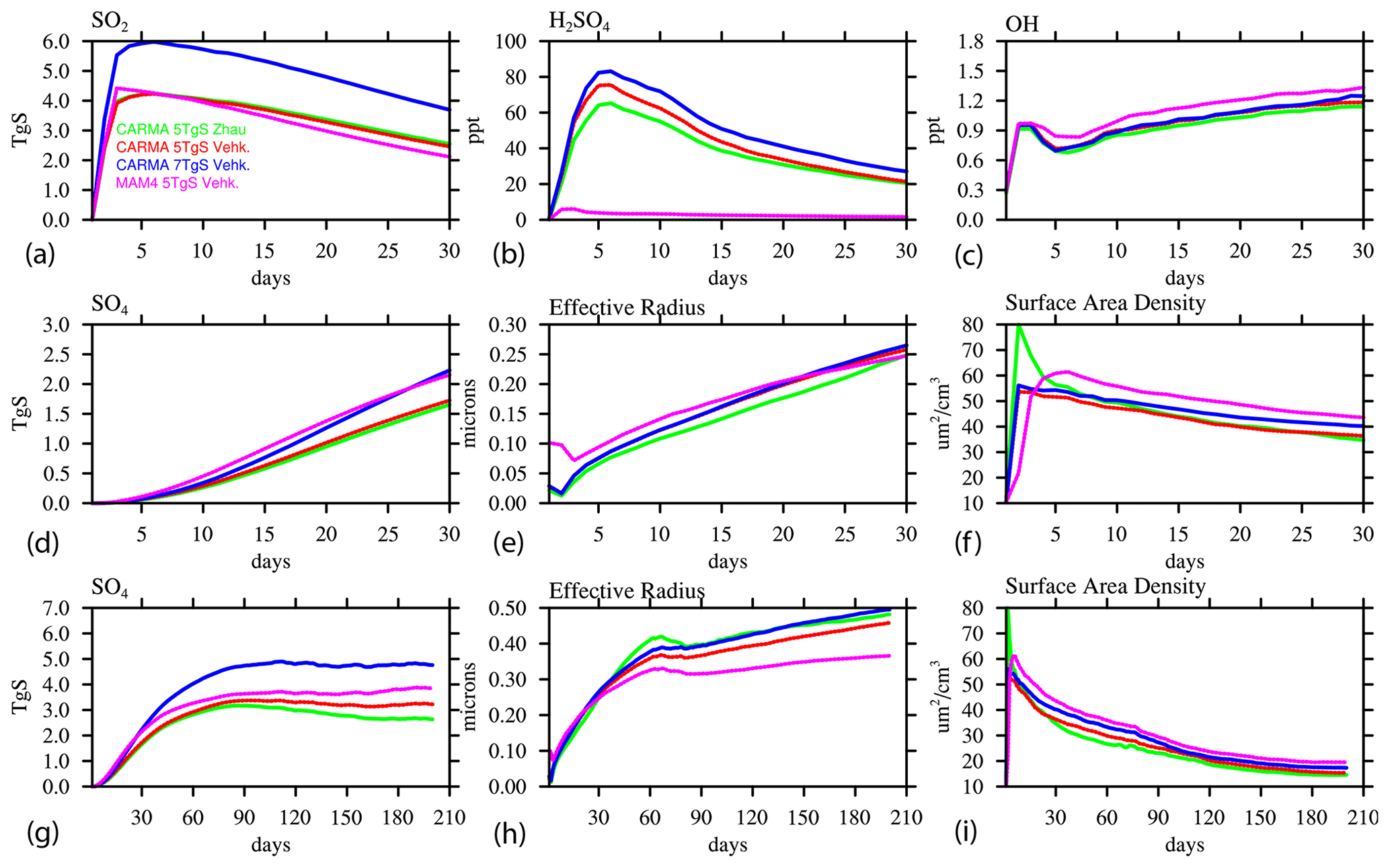
Figure A1Time series of air masses in the volcanic plume between 30∘ N and 30∘ S and between 200 and 5 hPa, as defined by grid points with a stratospheric surface area density larger than 0.1 µm, using daily averaged model output for different chemistry and aerosol variables, over the first 30 d (a–c and d–f) and over the first 6.5 months (g–i). This enables a comparison of the WACCM-MA experiments that compare the different nucleation schemes and injection amounts using CARMA and MAM4.
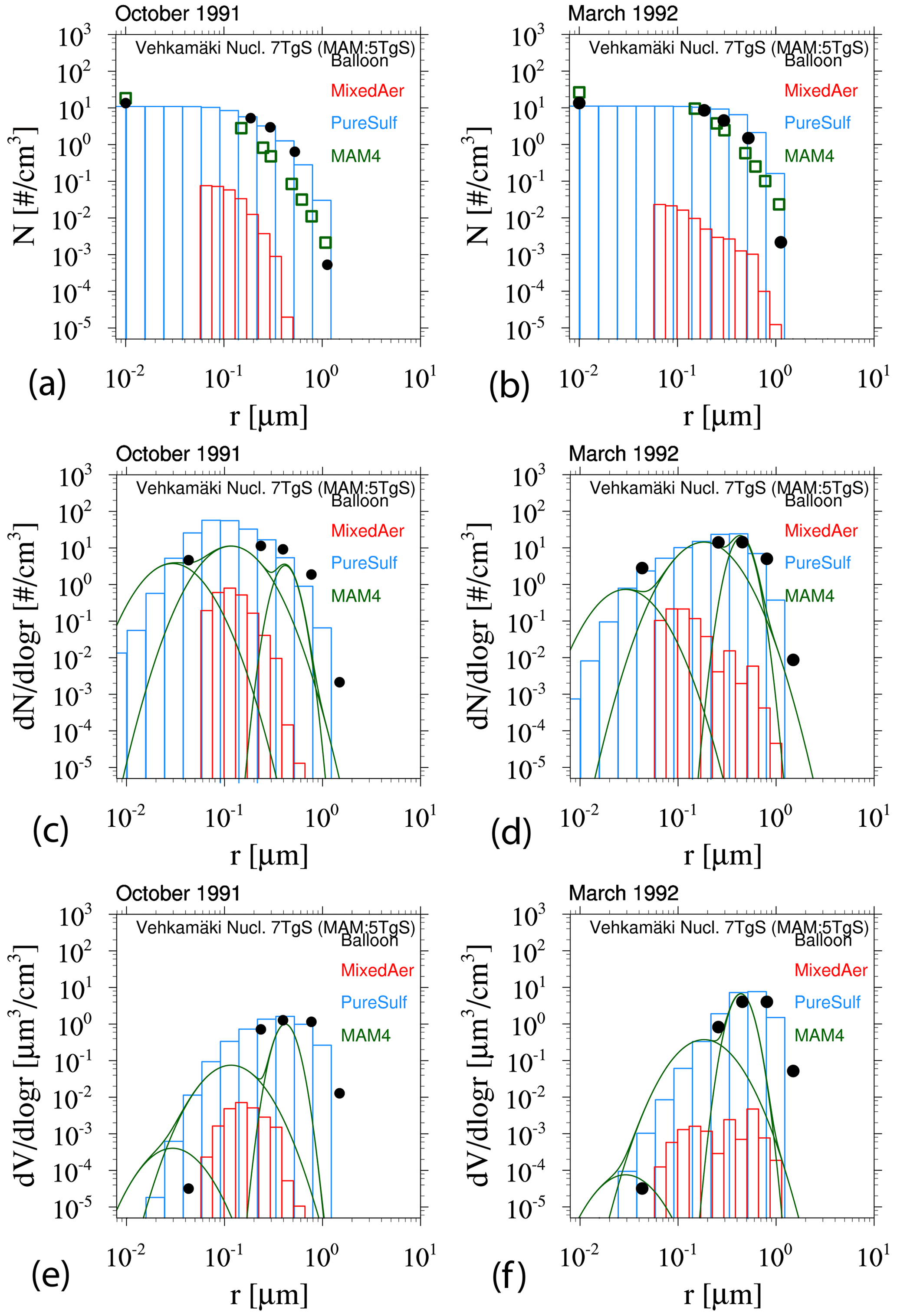
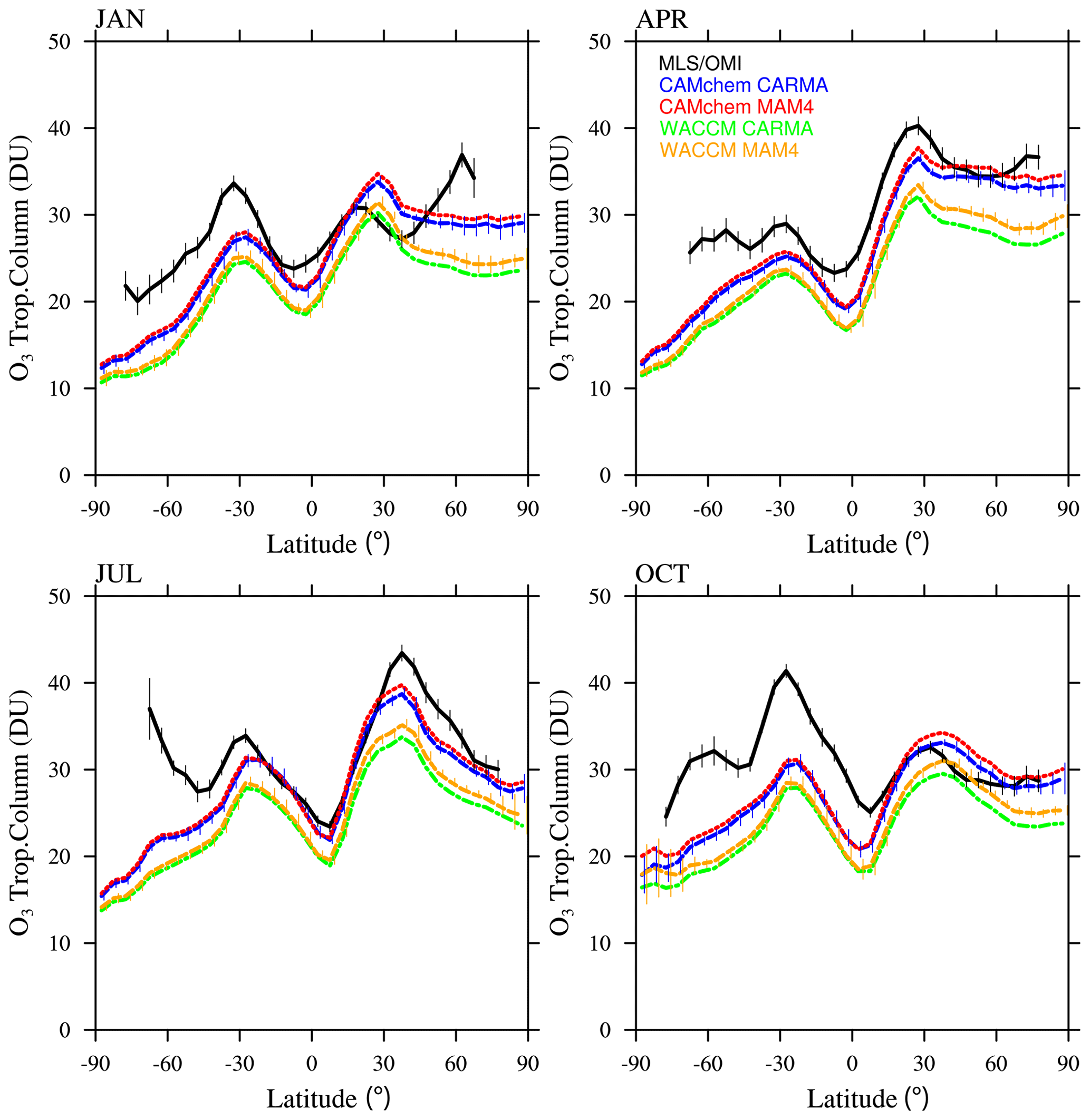
Figure A3As in Fig. 10 but for tropospheric ozone column (in DU; for ozone >150 ppb in the model).
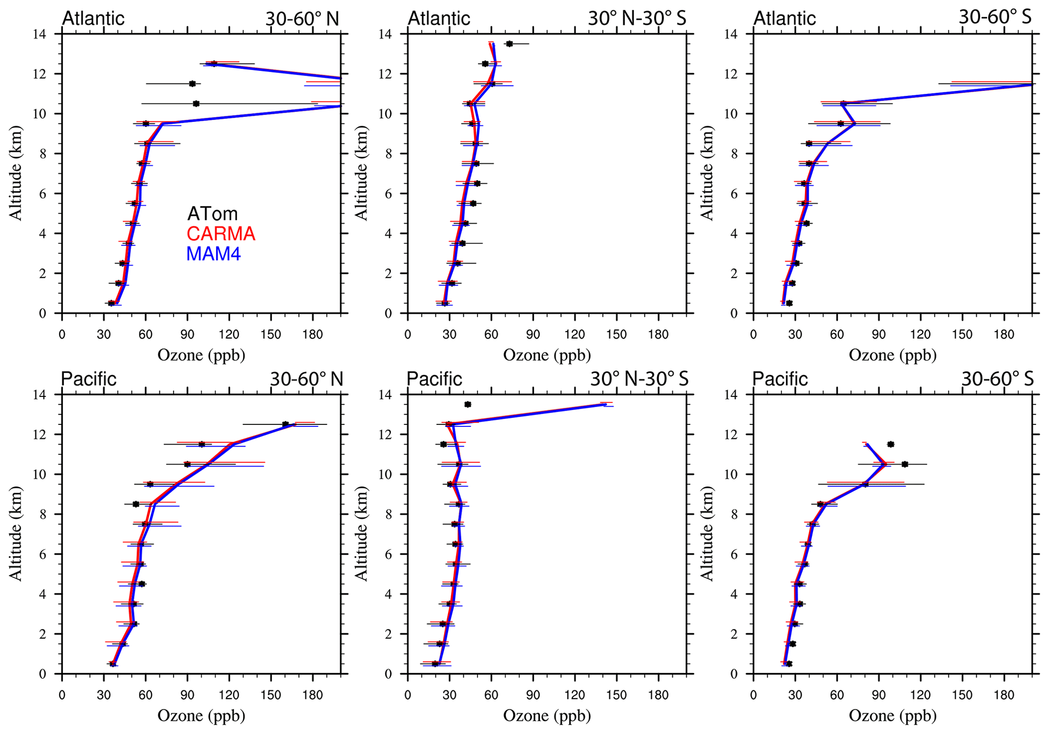
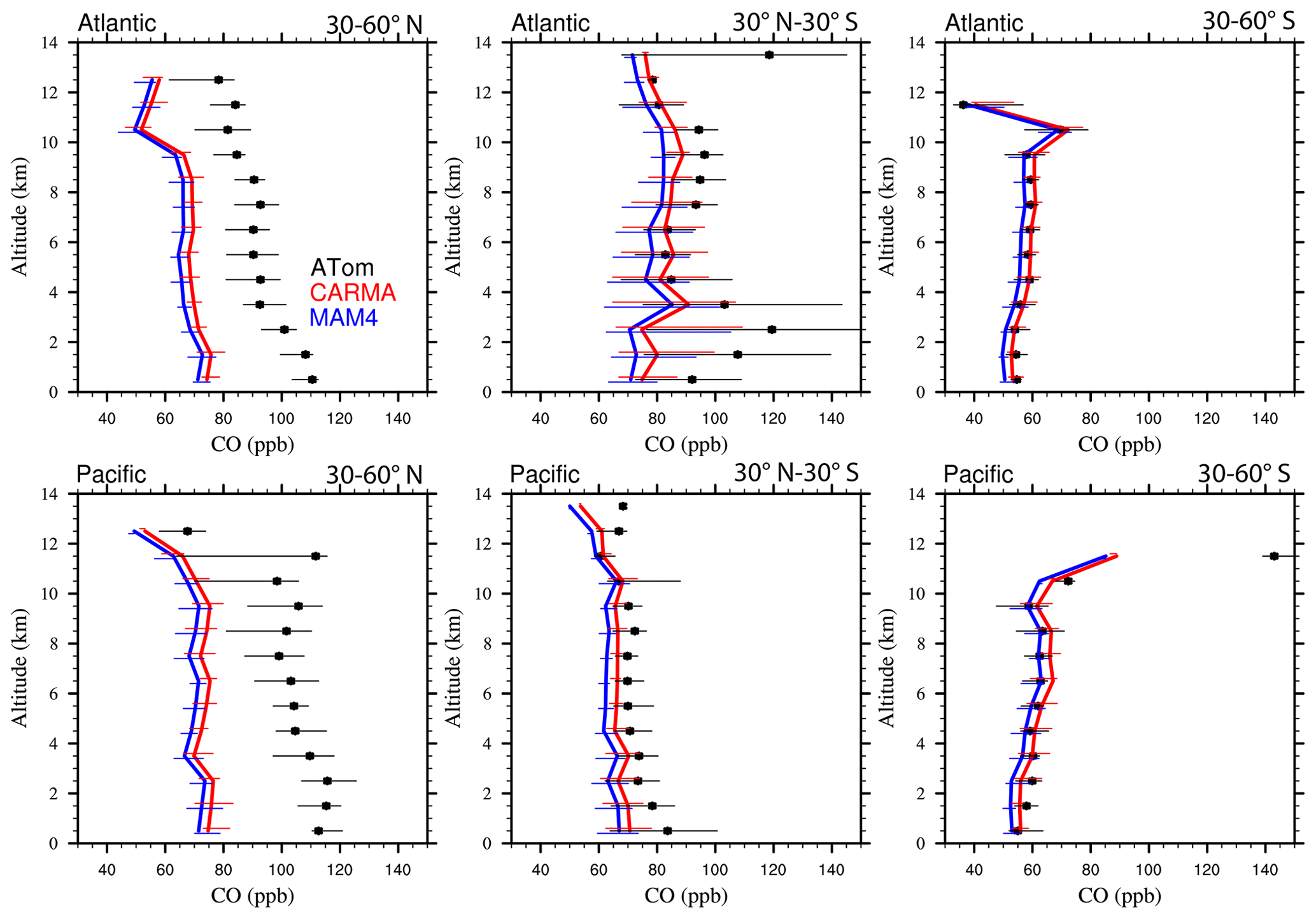
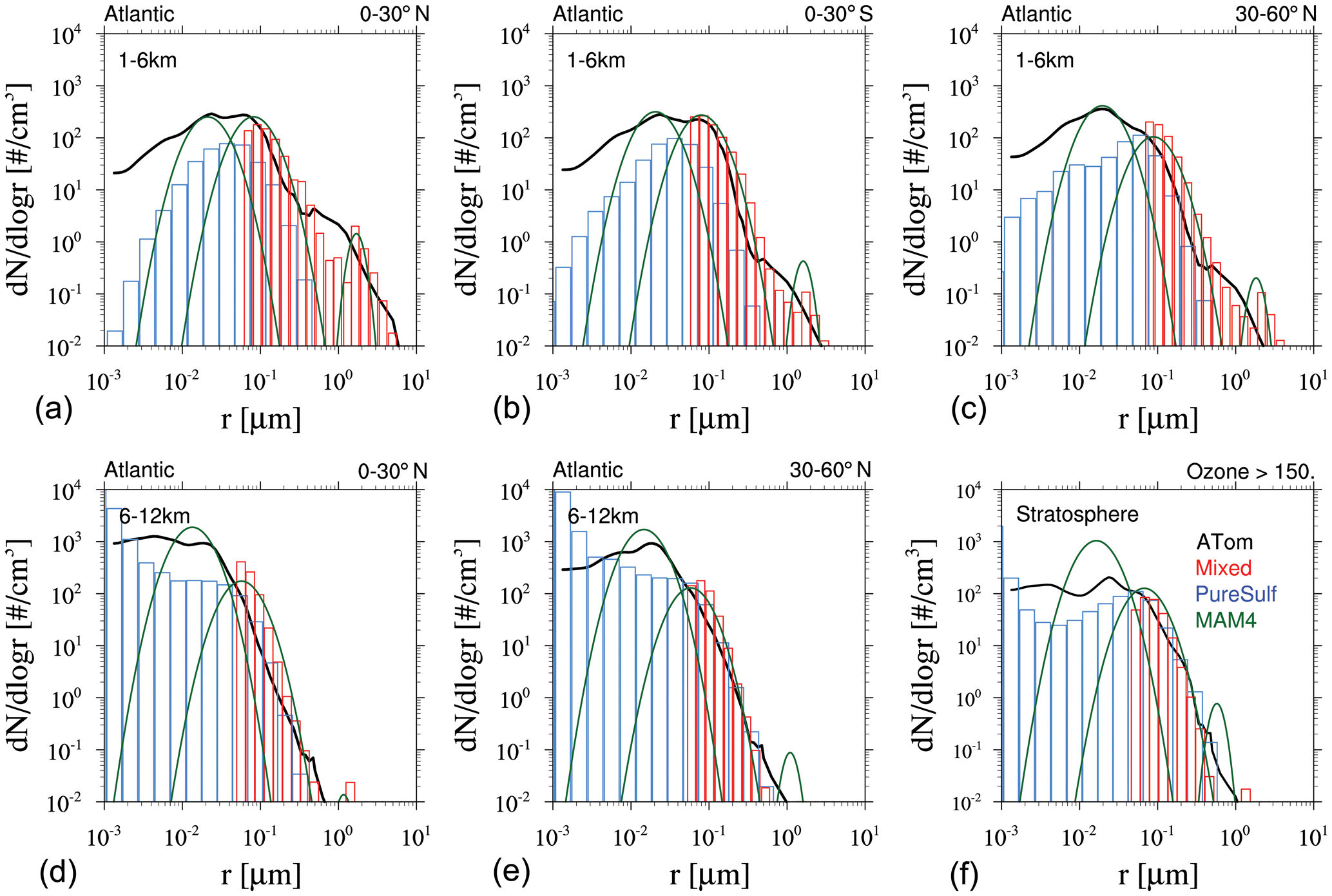
Figure A6Number density distributions of CAMchem CARMA results using the Vehkamäki aerosol nucleation scheme (instead of the Zhao nucleation scheme shown in Fig. 19) for size bins of the mixed aerosol (red) and pure sulfate (blue) group. Also shown are the CAMchem MAM4 modes (green lines) for ATom1 to ATom4 number size distributions from aircraft observations (black), which are averaged over three regions (0–30∘ N, 0–30∘ S, and 30–60∘ N) and over 1–6 km altitude (a–c), 6–12 km (d–e), and for stratospheric air masses with ozone mixing ratios >150 ppb (f). The model results were saved on the flight track using the closest location of each 1 min data point and then averaged over the same regions as the observations.
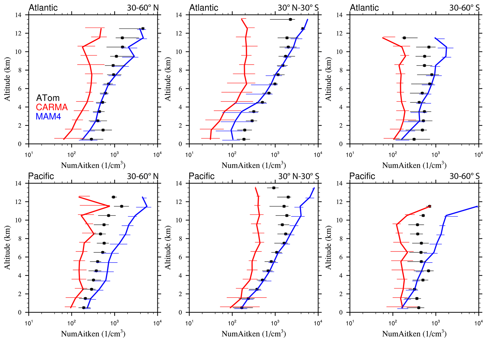
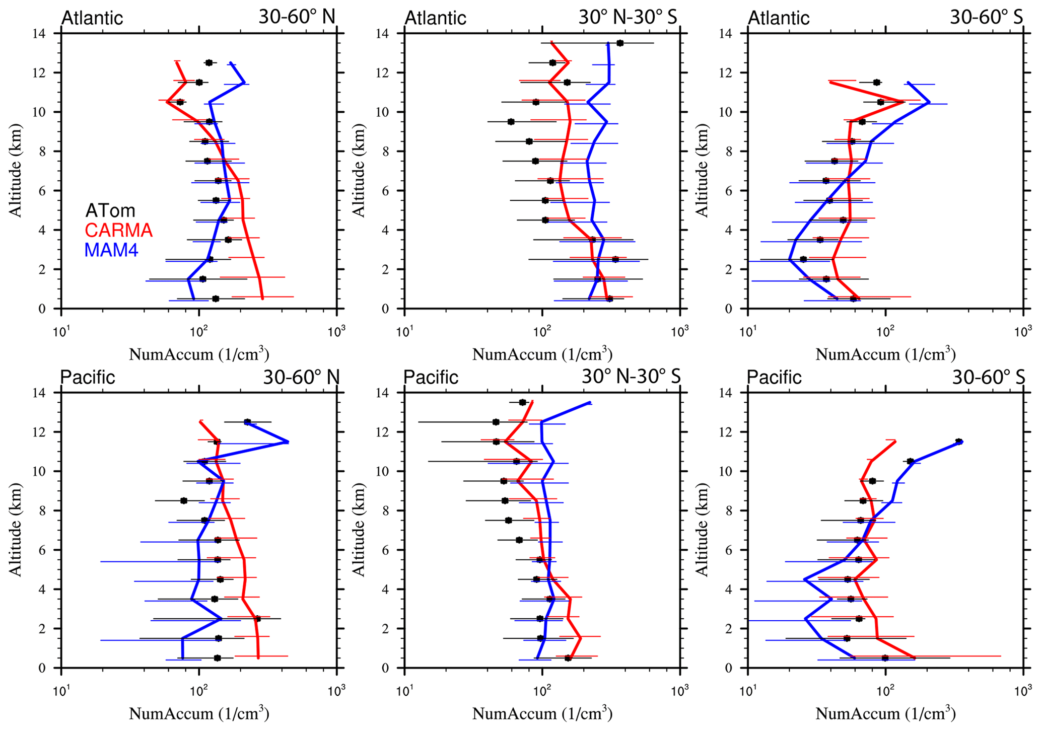
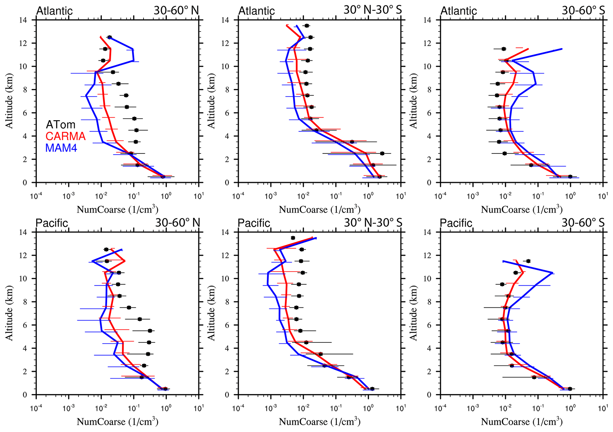
The code of the model used in this work is available through Zenodo (https://doi.org/10.5281/zenodo.7829697, Vitt and the CESM CARMA Development Team, 2023) and GitHub (git clone -b carma-trop-strat12, https://github.com/fvitt/CAM.git, last access: 14 April 2023). Model results used in this study are available for download upon request to the authors. The Wyoming balloon data used in this study are available in the data repository at the University of Wyoming Libraries (https://doi.org/10.15786/21534894, Deshler, 2022). MODIS data used for this study are available online (MOD08-M3.061 – MODIS/Terra Aerosol Cloud Water Vapor Ozone Monthly L3 Global 1Deg AOD 550 dark target deep blue combined mean; https://ladsweb.modaps.eosdis.nasa.gov/archive/allData/61/MOD08_M3/, last access: March 2023).
ST, MJM, YZ, FV, CGB, and PY developed and implemented the model. ST, MJM, and YZ performed model simulations and analyzed the results. DF produced comparison plots with MODIS data. TD helped with analyzing Wyoming balloon observations. ST led the writing of the paper, with valuable comments and discussions by all co-authors.
At least one of the (co-)authors is a member of the editorial board of Geoscientific Model Development. The peer-review process was guided by an independent editor, and the authors also have no other competing interests to declare.
Publisher’s note: Copernicus Publications remains neutral with regard to jurisdictional claims made in the text, published maps, institutional affiliations, or any other geographical representation in this paper. While Copernicus Publications makes every effort to include appropriate place names, the final responsibility lies with the authors.
We thank Daniele Visioni and Louisa Emmons, for helpful comments and suggestions, and Ulrike Niemeier, for providing helpful advice on plotting routines. This project has received funding from NOAA Climate Program Office Earth's Radiation Budget (grant nos. 03-01-07-001 and NA22OAR4310477). The Wyoming balloon measurements were completed under support from the National Science Foundation (NSF). The CESM project has been supported primarily by the National Science Foundation. This material is based upon work supported by the National Center for Atmospheric Research, which is a major facility sponsored by the NSF (grant no. 1852977). Computing and data storage resources, including the Cheyenne supercomputer (https://doi.org/10.5065/D6RX99HX, Cheyenne Supercomputer, 2021), were provided by the Computational and Information Systems Laboratory (CISL) at the National Center for Atmospheric Research (NCAR).
This research has been supported by the National Oceanic and Atmospheric Administration (grant no. 03-01-07-001 and NA22OAR4310477) and the National Science Foundation (grant no. 1852977).
This paper was edited by Samuel Remy and reviewed by two anonymous referees.
Abdul-Razzak, H. and Ghan, J.: Dri Dw, J. Geophys. Res., 105, 6837–6844, 2000. a, b
Adebiyi, A. A. and Kok, J. F.: Climate models miss most of the coarse dust in the atmosphere, Science Advances, 6, eaaz9507, https://doi.org/10.1126/sciadv.aaz9507, 2020. a
Bardeen, C. G., Toon, O. B., Jensen, E. J., Marsh, D. R., and Harvey, V. L.: Numerical simulations of the three-dimensional distribution of meteoric dust in the mesosphere and upper stratosphere, J. Geophys. Res., 113, D17202, https://doi.org/10.1029/2007JD009515, 2008. a
Bardeen, C. G., Toon, O. B., Jensen, E. J., Hervig, M. E., Randall, C. E., Benze, S., Marsh, D. R., and Merkel, A.: Numerical simulations of the three-dimensional distribution of polar mesospheric clouds and comparisons with Cloud Imaging and Particle Size (CIPS) experiment and the Solar Occultation For Ice Experiment (SOFIE) observations, J. Geophys. Res., 115, D10204, https://doi.org/10.1029/2009JD012451, 2010. a
Bardeen, C. G., Gettelman, a., Jensen, E. J., Heymsfield, a., Conley, a. J., Delanoë, J., Deng, M., and Toon, O. B.: Improved cirrus simulations in a general circulation model using CARMA sectional microphysics, J. Geophys. Res.-Atmos., 118, 11679–11697, https://doi.org/10.1002/2013JD020193, 2013. a
Barth, M. C., Rasch, P. J., Kiehl, J. T., Benkovitz, C. M., and Schwartz, S. E.: Sulfur chemistry in the National Center for Atmospheric Research Community Climate Model: Description, evaluation, features, and sensitivity to aqueous chemistry, J. Geophys. Res.-Atmos., 105, 1387–1415, https://doi.org/10.1029/1999JD900773, 2000. a, b
Binkowski, F. S. and Shankar, U.: The Regional Particulate Matter Model: 1. Model description and preliminary results, J. Geophys. Res., 100, 26191, https://doi.org/10.1029/95JD02093, 1995. a
Bogenschutz, P. A., Gettelman, A., Morrison, H., Larson, V. E., Schanen, D. P., Meyer, N. R., and Craig, C.: Unified parameterization of the planetary boundary layer and shallow convection with a higher-order turbulence closure in the Community Atmosphere Model: single-column experiments, Geosci. Model Dev., 5, 1407–1423, https://doi.org/10.5194/gmd-5-1407-2012, 2012. a
Brock, C. A., Froyd, K. D., Dollner, M., Williamson, C. J., Schill, G., Murphy, D. M., Wagner, N. J., Kupc, A., Jimenez, J. L., Campuzano-Jost, P., Nault, B. A., Schroder, J. C., Day, D. A., Price, D. J., Weinzierl, B., Schwarz, J. P., Katich, J. M., Wang, S., Zeng, L., Weber, R., Dibb, J., Scheuer, E., Diskin, G. S., DiGangi, J. P., Bui, T., Dean-Day, J. M., Thompson, C. R., Peischl, J., Ryerson, T. B., Bourgeois, I., Daube, B. C., Commane, R., and Wofsy, S. C.: Ambient aerosol properties in the remote atmosphere from global-scale in situ measurements, Atmos. Chem. Phys., 21, 15023–15063, https://doi.org/10.5194/acp-21-15023-2021, 2021. a, b
Buchard, V., Randles, C. A., da Silva, A. M., Darmenov, A., Colarco, P. R., Govindaraju, R., Ferrare, R., Hair, J., Beyersdorf, A. J., Ziemba, L. D., and Yu, H.: The MERRA-2 Aerosol Reanalysis, 1980 Onward. Part II: Evaluation and Case Studies, J. Climate, 30, 6851–6872, https://doi.org/10.1175/JCLI-D-16-0613.1, 2017. a
Carn, S., Clarisse, L., and Prata, A.: Multi-decadal satellite measurements of global volcanic degassing, J. Volcanol. Geoth. Res., 311, 99–134, https://doi.org/10.1016/j.jvolgeores.2016.01.002, 2016. a, b
Cheyenne Supercomputer: Computational and Information System Labroatory (CISL) at the National Center for Atmospheric Research (NCAR), https://doi.org/10.5065/D6RX99HX, 2021. a
Chin, M., Ginoux, P., Kinne, S., Torres, O., Holben, B. N., Duncan, B. N., Martin, R. V., Logan, J. A., Higurashi, A., and Nakajima, T.: Tropospheric Aerosol Optical Thickness from the GOCART Model and Comparisons with Satellite and Sun Photometer Measurements, J. Atmos. Sci., 59, 461–483, https://doi.org/10.1175/1520-0469(2002)059<0461:TAOTFT>2.0.CO;2, 2002. a
Colarco, P., Da Silva, A., Chin, M., and Diehl, T.: Online simulations of global aerosol distributions in the NASA GEOS-4 model and comparisons to satellite and ground-based aerosol optical depth, J. Geophys. Res.-Atmos., 115, D14207, https://doi.org/10.1029/2009JD012820, 2010. a
Danabasoglu, G., Lamarque, J.-F., Bachmeister, J., et al.: The Community Earth System Model version 2 (CESM2), J. Adv. Model. Earth Sy., 12, e2019MS001916, https://doi.org/10.1029/2019MS001916, 2020. a, b
Darmenov, A. S., da Silvia, A., and Koster, R. D.: The Quick Fire Emissions Dataset (QFED): Documentation of Versions 2.1, 2.2 and 2.4. Volume 38; Technical Report Series on Global Modeling and Data Assimilation, Tech. Rep., NASA Goddard Space Flight Center, Greenbelt, MD, United States, https://ntrs.nasa.gov/search.jsp?R=20180005253 (last access: 12 September 2018), 2015. a
Davis, N. A., Callaghan, P., Simpson, I. R., and Tilmes, S.: Specified dynamics scheme impacts on wave-mean flow dynamics, convection, and tracer transport in CESM2 (WACCM6), Atmos. Chem. Phys., 22, 197–214, https://doi.org/10.5194/acp-22-197-2022, 2022. a
Davis, N. A., Visioni, D., Garcia, R. R., Kinnison, D. E., Marsh, D. R., Mills, M. J., Richter, J. H., Tilmes, S., Bardeen, C., Gettelman, A., and Glanville, A. A.: Climate, variability, and climate sensitivity of “Middle Atmosphere” chemistry configurations of the Community Earth System Model Version 2, Whole Atmosphere Community Climate Model Version 6 (CESM2(WACCM6)), Authorea, https://doi.org/10.22541/essoar.167117634.40175082/v1, 2022. a, b, c, d, e
Deshler, T.: Mid Latitude | University of Wyoming Stratospheric Aerosol Measurements, University of Wyoming [data set], https://doi.org/10.15786/21534894.v4, 2022. a
Deshler, T., Larsen, N., Weissner, C., Schreiner, J., Mauersberger, K., Cairo, F., Adriani, A., Di Donfrancesco, G., Ovarlez, J., Ovarlez, H., Blum, U., Fricke, K. H., and Dörnbrack, A.: Large nitric acid particles at the top of an Arctic stratospheric cloud, J. Geophys. Res., 108, 4517, https://doi.org/10.1029/2003JD003479, 2003. a, b
Deshler, T., Luo, B., Kovilakam, M., Peter, T., and Kalnajs, L. E.: Retrieval of Aerosol Size Distributions From In Situ Particle Counter Measurements: Instrument Counting Efficiency and Comparisons With Satellite Measurements, J. Geophys. Res.-Atmos., 124, 5058–5087, https://doi.org/10.1029/2018JD029558, 2019. a
Easter, R. C., Ghan, S. J., Zhang, Y., Saylor, R. D., Chapman, E. G., Laulainen, N. S., Abdul-Razzak, H., Leung, L. R., Bian, X., and Zaveri, R. A.: MIRAGE: Model description and evaluation of aerosols and trace gases, J. Geophys. Res.-Atmos., 109, D20210, https://doi.org/10.1029/2004JD004571, 2004. a
Emmons, L. K., Schwantes, R. H., Orlando, J. J., Tyndall, G., Kinnison, D., Lamarque, J., Marsh, D., Mills, M. J., Tilmes, S., Bardeen, C., Buchholz, R. R., Conley, A., Gettelman, A., Garcia, R., Simpson, I., Blake, D. R., Meinardi, S., and Pétron, G.: The Chemistry Mechanism in the Community Earth System Model Version 2 (CESM2), J. Adv. Model. Earth Sy., 12, e2019MS001882, https://doi.org/10.1029/2019MS001882, 2020. a, b, c
English, J. M., Toon, O. B., Mills, M. J., and Yu, F.: Microphysical simulations of new particle formation in the upper troposphere and lower stratosphere, Atmos. Chem. Phys., 11, 9303–9322, https://doi.org/10.5194/acp-11-9303-2011, 2011. a
English, J. M., Toon, O. B., and Mills, M. J.: Microphysical simulations of sulfur burdens from stratospheric sulfur geoengineering, Atmos. Chem. Phys., 12, 4775–4793, https://doi.org/10.5194/acp-12-4775-2012, 2012. a, b, c, d, e, f, g
English, J. M., Toon, O. B., and Mills, M. J.: Microphysical simulations of large volcanic eruptions: Pinatubo and Toba, J. Geophys. Res.-Atmos., 118, 1880–1895, https://doi.org/10.1002/jgrd.50196, 2013. a
Fan, T. and Toon, O. B.: Modeling sea-salt aerosol in a coupled climate and sectional microphysical model: mass, optical depth and number concentration, Atmos. Chem. Phys., 11, 4587–4610, https://doi.org/10.5194/acp-11-4587-2011, 2011. a, b
Fiore, A. M., Naik, V., and Leibensperger, E. M.: Air Quality and Climate Connections, J. Air Waste Manage., 65, 645–685, https://doi.org/10.1080/10962247.2015.1040526, 2015. a
Fisher, B. L., Krotkov, N. A., Bhartia, P. K., Li, C., Carn, S. A., Hughes, E., and Leonard, P. J. T.: A new discrete wavelength backscattered ultraviolet algorithm for consistent volcanic SO2 retrievals from multiple satellite missions, Atmos. Meas. Tech., 12, 5137–5153, https://doi.org/10.5194/amt-12-5137-2019, 2019. a, b, c
Gao, R.-S., Rosenlof, K. H., Kärcher, B., Tilmes, S., Toon, O. B., Maloney, C., and Yu, P.: Toward practical stratospheric aerosol albedo modification: Solar-powered lofting, Science Advances, 7, eabe3416, https://doi.org/10.1126/sciadv.abe3416, 2021. a
Gaubert, B., Bouarar, I., Doumbia, T., Liu, Y., Stavrakou, T., Deroubaix, A., Darras, S., Elguindi, N., Granier, C., Lacey, F., Müller, J., Shi, X., Tilmes, S., Wang, T., and Brasseur, G. P.: Global Changes in Secondary Atmospheric Pollutants During the 2020 COVID‐19 Pandemic, J. Geophys. Res.-Atmos., 126, e2020JD034213, https://doi.org/10.1029/2020JD034213, 2021. a
Gettelman, A. and Morrison, H.: Advanced Two-Moment Bulk Microphysics for Global Models. Part I: Off-Line Tests and Comparison with Other Schemes, J. Climate, 28, 1268–1287, https://doi.org/10.1175/JCLI-D-14-00102.1, 2015. a, b
Gettelman, A., Mills, M. J., Kinnison, D. E., Garcia, R. R., Smith, A. K., Marsh, D. R., Tilmes, S., Vitt, F., Bardeen, C. G., McInerney, J., Liu, H.-L., Solomon, S. C., Polvani, L. M., Emmons, L. K., Lamarque, J.-F., Richter, J. H., Glanville, A. S., Bacmeister, J. T., Phillips, A. S., Neale, R. B., Simpson, I. R., DuVivier, A. K., Hodzic, A., and Randel, W. J.: The Whole Atmosphere Community Climate Model Version 6 (WACCM6), J. Geophys. Res.-Atmos., 124, 12380–12403, https://doi.org/10.1029/2019JD030943, 2019. a, b, c, d
Ghan, S. J. and Zaveri, R. A.: Parameterization of optical properties for hydrated internally mixed aerosol, J. Geophys. Res.-Atmos., 112, D10201, https://doi.org/10.1029/2006JD007927, 2007. a, b
Gillette, D. A. and Passi, R.: Modeling Dust Emission Caused by Wind Erosion, J. Geophys. Res.-Atmos, 93, 14233–14242, 1988. a
Guenther, A. B., Jiang, X., Heald, C. L., Sakulyanontvittaya, T., Duhl, T., Emmons, L. K., and Wang, X.: The Model of Emissions of Gases and Aerosols from Nature version 2.1 (MEGAN2.1): an extended and updated framework for modeling biogenic emissions, Geosci. Model Dev., 5, 1471–1492, https://doi.org/10.5194/gmd-5-1471-2012, 2012. a
Guo, S., Bluth, G. J. S., Rose, W. I., Watson, I. M., and Prata, A. J.: Re-evaluation of SO2 release of the 15 June 1991 Pinatubo eruption using ultraviolet and infrared satellite sensors, Geochem. Geophy. Geosy., 5, Q04001, https://doi.org/10.1029/2003GC000654, 2004. a
Hodzic, A., Madronich, S., Kasibhatla, P. S., Tyndall, G., Aumont, B., Jimenez, J. L., Lee-Taylor, J., and Orlando, J.: Organic photolysis reactions in tropospheric aerosols: effect on secondary organic aerosol formation and lifetime, Atmos. Chem. Phys., 15, 9253–9269, https://doi.org/10.5194/acp-15-9253-2015, 2015. a
Hodzic, A., Kasibhatla, P. S., Jo, D. S., Cappa, C. D., Jimenez, J. L., Madronich, S., and Park, R. J.: Rethinking the global secondary organic aerosol (SOA) budget: stronger production, faster removal, shorter lifetime, Atmos. Chem. Phys., 16, 7917–7941, https://doi.org/10.5194/acp-16-7917-2016, 2016. a
Iacono, M. J., Delamere, J. S., Mlawer, E. J., Shephard, M. W., Clough, S. A., and Collins, W. D.: Radiative forcing by long-lived greenhouse gases: Calculations with the AER radiative transfer models, J. Geophys. Res., 113, D13103, https://doi.org/10.1029/2008JD009944, 2008. a
Jo, D. S., Hodzic, A., Emmons, L. K., Tilmes, S., Schwantes, R. H., Mills, M. J., Campuzano-Jost, P., Hu, W., Zaveri, R. A., Easter, R. C., Singh, B., Lu, Z., Schulz, C., Schneider, J., Shilling, J. E., Wisthaler, A., and Jimenez, J. L.: Future changes in isoprene-epoxydiol-derived secondary organic aerosol (IEPOX SOA) under the Shared Socioeconomic Pathways: the importance of physicochemical dependency, Atmos. Chem. Phys., 21, 3395–3425, https://doi.org/10.5194/acp-21-3395-2021, 2021. a, b
Jo, D. S., Tilmes, S., Emmons, L. K., Wang, S., and Vitt, F.: A new simplified parameterization of secondary organic aerosol in the Community Earth System Model Version 2 (CESM2; CAM6.3), Geosci. Model Dev., 16, 3893–3906, https://doi.org/10.5194/gmd-16-3893-2023, 2023. a
Kerminen, V. M. and Kulmala, M.: Analytical formulae connecting the “real” and the “apparent” nucleation rate and the nuclei number concentration for atmospheric nucleation events, J. Aerosol Sci., 33, 609–622, https://doi.org/10.1016/S0021-8502(01)00194-X, 2002. a
Knote, C., Hodzic, A., Jimenez, J. L., Volkamer, R., Orlando, J. J., Baidar, S., Brioude, J., Fast, J., Gentner, D. R., Goldstein, A. H., Hayes, P. L., Knighton, W. B., Oetjen, H., Setyan, A., Stark, H., Thalman, R., Tyndall, G., Washenfelder, R., Waxman, E., and Zhang, Q.: Simulation of semi-explicit mechanisms of SOA formation from glyoxal in aerosol in a 3-D model, Atmos. Chem. Phys., 14, 6213–6239, https://doi.org/10.5194/acp-14-6213-2014, 2014. a
Kok, J. F.: A scaling theory for the size distribution of emitted dust aerosols suggests climate models underestimate the size of the global dust cycle, P. Natl. Acad. Sci. USA, 108, 1016–1021, https://doi.org/10.1073/pnas.1014798108, 2011. a
Kokkola, H., Kühn, T., Laakso, A., Bergman, T., Lehtinen, K. E. J., Mielonen, T., Arola, A., Stadtler, S., Korhonen, H., Ferrachat, S., Lohmann, U., Neubauer, D., Tegen, I., Siegenthaler-Le Drian, C., Schultz, M. G., Bey, I., Stier, P., Daskalakis, N., Heald, C. L., and Romakkaniemi, S.: SALSA2.0: The sectional aerosol module of the aerosol–chemistry–climate model ECHAM6.3.0-HAM2.3-MOZ1.0, Geosci. Model Dev., 11, 3833–3863, https://doi.org/10.5194/gmd-11-3833-2018, 2018. a
Kremser, S., Thomason, L. W., von Hobe, M., Hermann, M., Deshler, T., Timmreck, C., Toohey, M., Stenke, A., Schwarz, J. P., Weigel, R., Fueglistaler, S., Prata, F. J., Vernier, J.-P., Schlager, H., Barnes, J. E., Antuña-Marrero, J.-C., Fairlie, D., Palm, M., Mahieu, E., Notholt, J., Rex, M., Bingen, C., Vanhellemont, F., Bourassa, A., Plane, J. M. C., Klocke, D., Carn, S. A., Clarisse, L., Trickl, T., Neely, R., James, A. D., Rieger, L., Wilson, J. C., and Meland, B.: Stratospheric aerosol-Observations, processes, and impact on climate, Rev. Geophys., 54, 278–335, https://doi.org/10.1002/2015RG000511, 2016. a
Levy, R. C., Mattoo, S., Munchak, L. A., Remer, L. A., Sayer, A. M., Patadia, F., and Hsu, N. C.: The Collection 6 MODIS aerosol products over land and ocean, Atmos. Meas. Tech., 6, 2989–3034, https://doi.org/10.5194/amt-6-2989-2013, 2013. a
Li, L., Mahowald, N. M., Kok, J. F., Liu, X., Wu, M., Leung, D. M., Hamilton, D. S., Emmons, L. K., Huang, Y., Sexton, N., Meng, J., and Wan, J.: Importance of different parameterization changes for the updated dust cycle modeling in the Community Atmosphere Model (version 6.1), Geosci. Model Dev., 15, 8181–8219, https://doi.org/10.5194/gmd-15-8181-2022, 2022. a
Lian, S., Zhou, L., Murphy, D. M., Froyd, K. D., Toon, O. B., and Yu, P.: Global distribution of Asian, Middle Eastern, and North African dust simulated by CESM1/CARMA, Atmos. Chem. Phys., 22, 13659–13676, https://doi.org/10.5194/acp-22-13659-2022, 2022. a, b
Liu, X. and Penner, J. E.: Ice nucleation parameterization for global models, Meteorol. Z., 14, 499–514, https://doi.org/10.1127/0941-2948/2005/0059, 2005. a
Liu, X., Penner, J. E., Ghan, S. J., and Wang, M.: Inclusion of ice microphysics in the NCAR Community Atmospheric Model version 3 (CAM3), J. Climate, 20, 4526–4547, https://doi.org/10.1175/JCLI4264.1, 2007. a
Liu, X., Easter, R. C., Ghan, S. J., Zaveri, R., Rasch, P., Shi, X., Lamarque, J.-F., Gettelman, A., Morrison, H., Vitt, F., Conley, A., Park, S., Neale, R., Hannay, C., Ekman, A. M. L., Hess, P., Mahowald, N., Collins, W., Iacono, M. J., Bretherton, C. S., Flanner, M. G., and Mitchell, D.: Toward a minimal representation of aerosols in climate models: description and evaluation in the Community Atmosphere Model CAM5, Geosci. Model Dev., 5, 709–739, https://doi.org/10.5194/gmd-5-709-2012, 2012. a, b, c
Liu, X., Ma, P.-L., Wang, H., Tilmes, S., Singh, B., Easter, R. C., Ghan, S. J., and Rasch, P. J.: Description and evaluation of a new four-mode version of the Modal Aerosol Module (MAM4) within version 5.3 of the Community Atmosphere Model, Geosci. Model Dev., 9, 505–522, https://doi.org/10.5194/gmd-9-505-2016, 2016. a, b, c
Lu, Z., Liu, X., Zaveri, R. A., Easter, R. C., Tilmes, S., Emmons, L. K., Vitt, F., Singh, B., Wang, H., Zhang, R., and Rasch, P. J.: Radiative Forcing of Nitrate Aerosols From 1975 to 2010 as Simulated by MOSAIC Module in CESM2‐MAM4, J. Geophys. Res.-Atmos., 126, https://doi.org/10.1029/2021JD034809, 2021. a, b
Mårtensson, E. M., Nilsson, E. D., de Leeuw, G., Cohen, L. H., and Hansson, H. C.: Laboratory simulations and parameterization of the primary marine aerosol production, J. Geophys. Res.-Atmos., 108, 4297, https://doi.org/10.1029/2002jd002263, 2003. a
Mayers, M. P., DeMott, P. J., and Cotton, W. R.: New Primary Ice-Nuclation Parammeterization in an Explicit Cloud Model, J. Appl. Meteorol., 31, 88–100, 1992. a
Mills, M. J., Schmidt, A., Easter, R., Solomon, S., Kinnison, D. E., Ghan, S. J., Neely, R. R., Marsh, D. R., Conley, A., Bardeen, C. G., and Gettelman, A.: Global volcanic aerosol properties derived from emissions, 1990–2014, using CESM1(WACCM), J. Geophys. Res.-Atmos., 121, 2332–2348, https://doi.org/10.1002/2015JD024290, 2016. a, b, c, d, e, f, g, h, i
Mills, M. J., Richter, J. H., Tilmes, S., Kravitz, B., MacMartin, D. G., Glanville, A. A., Tribbia, J. J., Lamarque, J.-F., Vitt, F., Schmidt, A., Gettelman, A., Hannay, C., Bacmeister, J. T., and Kinnison, D. E.: Radiative and chemical response to interactive stratospheric sulfate aerosols in fully coupled CESM1(WACCM), J. Geophys. Res.-Atmos., 122, 13061–13078, https://doi.org/10.1002/2017JD027006, 2017. a, b, c
Monahan, E. C., Spiel, D. E., and Davidson, K. L.: A Model of Marine Aerosol Generation via Whitecaps and Wave Disruption, in: Oceanic whitecaps and their role in air-sea exchange processes, edited by: MacNiocaill, E. C. and M. G., R., 167–174, Dordrecht, NL, Online ISBN 978-94-009-4668-2, 1986. a
Murphy, D. M., Froyd, K. D., Bourgeois, I., Brock, C. A., Kupc, A., Peischl, J., Schill, G. P., Thompson, C. R., Williamson, C. J., and Yu, P.: Radiative and chemical implications of the size and composition of aerosol particles in the existing or modified global stratosphere, Atmos. Chem. Phys., 21, 8915–8932, https://doi.org/10.5194/acp-21-8915-2021, 2021. a, b, c
Neely III, R. R. and Schmidt, A.: VolcanEESM: Global volcanic sulphur dioxide (SO2) emissions database from 1850 to present, Centre for Environmental Data Analysis [data set], https://doi.org/10.5285/76ebdc0b-0eed-4f70-b89e-55e606bcd568, 2016. a, b
Niemeier, U., Schmidt, H., and Timmreck, C.: The dependency of geoengineered sulfate aerosol on the emission strategy, Atmos. Sci. Lett., 12, 189–194, https://doi.org/10.1002/asl.304, 2011. a, b
Petters, M. D. and Kreidenweis, S. M.: A single parameter representation of hygroscopic growth and cloud condensation nucleus activity, Atmos. Chem. Phys., 7, 1961–1971, https://doi.org/10.5194/acp-7-1961-2007, 2007. a
Pöschl, U., Canagaratna, M., Jayne, J. T., Molina, L. T., Worsnop, D. R., Kolb, C. E., and Molina, M. J.: Mass accommodation coefficient of H2SO4 vapor on aqueous sulfuric acid surfaces and gaseous diffusion coefficient of H2SO4 in , J. Phys. Chem. A, 102, 10082–10089, https://doi.org/10.1021/jp982809s, 1998. a
Quaglia, I., Timmreck, C., Niemeier, U., Visioni, D., Pitari, G., Brodowsky, C., Brühl, C., Dhomse, S. S., Franke, H., Laakso, A., Mann, G. W., Rozanov, E., and Sukhodolov, T.: Interactive stratospheric aerosol models' response to different amounts and altitudes of SO2 injection during the 1991 Pinatubo eruption, Atmos. Chem. Phys., 23, 921–948, https://doi.org/10.5194/acp-23-921-2023, 2023. a
Randles, C. A., da Silva, A. M., Buchard, V., Colarco, P. R., Darmenov, A., Govindaraju, R., Smirnov, A., Holben, B., Ferrare, R., Hair, J., Shinozuka, Y., and Flynn, C. J.: The MERRA-2 Aerosol Reanalysis, 1980 Onward. Part I: System Description and Data Assimilation Evaluation, J. Climate, 30, 6823–6850, https://doi.org/10.1175/JCLI-D-16-0609.1, 2017. a
Read, W. G., Froidevaux, L., and Waters, J. W.: Microwave limb sounder measurement of stratospheric SO2 from the Mt. Pinatubo Volcano, Geophys. Res. Lett., 20, 1299–1302, https://doi.org/10.1029/93GL00831, 1993. a
Santer, B. D., Bonfils, C., Painter, J. F., Zelinka, M. D., Mears, C., Solomon, S., Schmidt, G. A., Fyfe, J. C., Cole, J. N., Nazarenko, L., Taylor, K. E., and Wentz, F. J.: Volcanic contribution to decadal changes in tropospheric temperature, Nat. Geosci., 7, 185–189, https://doi.org/10.1038/ngeo2098, 2014. a
Seinfeld, J. H. and Pandis, S. N.: Atmospheric Chemistry and Physics, John Wiley and Sons, ISBN 9781119221166, 1998. a
Shan, Y., Liu, X., Lin, L., Ke, Z., and Lu, Z.: An Improved Representation of Aerosol Wet Removal by Deep Convection and Impacts on Simulated Aerosol Vertical Profiles, J. Geophys. Res.-Atmos., 126, https://doi.org/10.1029/2020JD034173, 2021. a, b
Su, L. and Toon, O. B.: Numerical simulations of asian dust storms using a coupled climate-aerosol microphysical model, J. Geophys. Res.-Atmos., 114, D14202, https://doi.org/10.1029/2008JD010956, 2009. a
Sukhodolov, T., Egorova, T., Stenke, A., Ball, W. T., Brodowsky, C., Chiodo, G., Feinberg, A., Friedel, M., Karagodin-Doyennel, A., Peter, T., Sedlacek, J., Vattioni, S., and Rozanov, E.: Atmosphere–ocean–aerosol–chemistry–climate model SOCOLv4.0: description and evaluation, Geosci. Model Dev., 14, 5525–5560, https://doi.org/10.5194/gmd-14-5525-2021, 2021. a
Tabazadeh, A., Toon, O. B., Clegg, S. L., and Hamill, P.: A new parameterization of aerosol composition: Atmospheric implications, Geophys. Res. Lett., 24, 1931–1934, https://doi.org/10.1029/97GL01879, 1997. a, b
Tang, W., Emmons, L. K., Buchholz, R. R., Wiedinmyer, C., Schwantes, R. H., He, C., Kumar, R., Pfister, G. G., Worden, H. M., Hornbrook, R. S., Apel, E. C., Tilmes, S., Gaubert, B., Martinez‐Alonso, S., Lacey, F., Holmes, C. D., Diskin, G. S., Bourgeois, I., Peischl, J., Ryerson, T. B., Hair, J. W., Weinheimer, A. J., Montzka, D. D., Tyndall, G. S., and Campos, T. L.: Effects of Fire Diurnal Variation and Plume Rise on U.S. Air Quality During FIREX‐AQ and WE‐CAN Based on the Multi‐Scale Infrastructure for Chemistry and Aerosols (MUSICAv0), J. Geophys. Res.-Atmos., 127, e2022JD036650, https://doi.org/10.1029/2022JD036650, 2022. a
Thomason, L. W., Ernest, N., Millán, L., Rieger, L., Bourassa, A., Vernier, J.-P., Manney, G., Luo, B., Arfeuille, F., and Peter, T.: A global space-based stratospheric aerosol climatology: 1979–2016, Earth Syst. Sci. Data, 10, 469–492, https://doi.org/10.5194/essd-10-469-2018, 2018. a
Tilmes, S., Lamarque, J.-F., Emmons, L. K., Kinnison, D. E., Ma, P.-L., Liu, X., Ghan, S., Bardeen, C., Arnold, S., Deeter, M., Vitt, F., Ryerson, T., Elkins, J. W., Moore, F., Spackman, J. R., and Val Martin, M.: Description and evaluation of tropospheric chemistry and aerosols in the Community Earth System Model (CESM1.2), Geosci. Model Dev., 8, 1395–1426, https://doi.org/10.5194/gmd-8-1395-2015, 2015. a
Tilmes, S., Richter, J. H., Mills, M. J., Kravitz, B., MacMartin, D. G., Garcia, R. R., Kinnison, D. E., Lamarque, J.-F., Tribbia, J., and Vitt, F.: Effects of different stratospheric SO2 injection altitudes on stratospheric chemistry and dynamics, J. Geophys. Res.-Atmos., 123, 4654–4673, 2018. a
Tilmes, S., Hodzic, A., Emmons, L. K., Mills, M. J., Gettelman, A., Kinnison, D. E., Park, M., Lamarque, J.-F., Vitt, F., Shrivastava, M., Jost, P. C., Jimenez, J., and Liu, X.: Climate forcing and trends of organic aerosols in the Community Earth System Model (CESM2), J. Adv. Model. Earth Sy., 11, 4323–4351, 2019. a, b
Toon, O. B. and Ackerman, T. P.: Algorithms for the calculation of scattering by stratified spheres, Applied Optics, 20, 3657–3660, https://doi.org/10.1364/ao.20.003657, 1981. a
Toon, O. B., Turco, R. P., Westphal, D., Malone, R., and Liu, M.: A Multidimensional Model for Aerosols: Description of Computational Analogs, J. Atmos. Sci., 45, 2123–2144, https://doi.org/10.1175/1520-0469(1988)045<2123:AMMFAD>2.0.CO;2, 1988. a
Toon, O. B., Turco, R. P., Jordan, J., Goodman, J., and Ferry, G.: Physical processes in polar stratospheric ice clouds, J. Geophys. Res., 94, 11359–11380, 1989. a
Vehkamäki, H., Kulmala, M., Napari, I., Lehtinen, K. E., Timmreck, C., Noppel, M., and Laaksonen, A.: An improved parameterization for sulfuric acid-water nucleation rates for tropospheric and stratospheric conditions, J. Geophys. Res.-Atmos., 107, AAC 3-1–AAC 3-10, https://doi.org/10.1029/2002JD002184, 2002. a, b, c
Vitt, F. and the CESM CARMA Development Team: fvitt/CAM: CARMA sectional aerosol microphysical model in CESM2 (carma_trop_strat12), Zenodo [data set], https://doi.org/10.5281/zenodo.7829697, 2023. a
Wang, H., Easter, R. C., Rasch, P. J., Wang, M., Liu, X., Ghan, S. J., Qian, Y., Yoon, J.-H., Ma, P.-L., and Vinoj, V.: Sensitivity of remote aerosol distributions to representation of cloud–aerosol interactions in a global climate model, Geosci. Model Dev., 6, 765–782, https://doi.org/10.5194/gmd-6-765-2013, 2013. a, b
Wang, Y., Liu, X., Hoose, C., and Wang, B.: Different contact angle distributions for heterogeneous ice nucleation in the Community Atmospheric Model version 5, Atmos. Chem. Phys., 14, 10411–10430, https://doi.org/10.5194/acp-14-10411-2014, 2014. a
Wiedinmyer, C., Akagi, S. K., Yokelson, R. J., Emmons, L. K., Al-Saadi, J. A., Orlando, J. J., and Soja, A. J.: The Fire INventory from NCAR (FINN): a high resolution global model to estimate the emissions from open burning, Geosci. Model Dev., 4, 625–641, https://doi.org/10.5194/gmd-4-625-2011, 2011. a
Williamson, D. L.: Time-split versus process-split coupling of parameterizations and dynamical core, Mon. Weather Rev., 130, 2024–2041, https://doi.org/10.1175/1520-0493(2002)130<2024:TSVPSC>2.0.CO;2, 2002. a
Wofsy, S.: ATom: Merged Atmospheric Chemistry, Trace Gases, and Aerosols, ORNL Distributed Active Archive Center [data set], https://doi.org/10.3334/ORNLDAAC/1925, 2018. a
Yu, P., Toon, O. B., Bardeen, C. G., Mills, M. J., Fan, T., English, J. M., and Neely, R. R.: Evaluations of tropospheric aerosol properties simulated by the community earth system model with a sectional aerosol microphysics scheme, J. Adv. Model. Earth Sy., 7, 865–914, https://doi.org/10.1002/2014MS000421, 2015. a, b, c, d, e, f, g, h, i, j, k, l, m, n, o, p, q
Yu, P., Murphy, D. M., Portmann, R. W., Toon, O. B., Froyd, K. D., Rollins, A. W., Gao, R., and Rosenlof, K. H.: Radiative forcing from anthropogenic sulfur and organic emissions reaching the stratosphere, Geophys. Res. Lett., 43, 9361–9367, https://doi.org/10.1002/2016GL070153, 2016. a
Yu, P., Rosenlof, K. H., Liu, S., Telg, H., Thornberry, T. D., Rollins, A. W., Portmann, R. W., Bai, Z., Ray, E. A., Duan, Y., Pan, L. L., Toon, O. B., Bian, J., and Gao, R.-S.: Efficient transport of tropospheric aerosol into the stratosphere via the Asian summer monsoon anticyclone, P. Natl. Acad. Sci., 114, 6972–6977, https://doi.org/10.1073/pnas.1701170114, 2017. a
Yu, P., Froyd, K. D., Portmann, R. W., Toon, O. B., Freitas, S. R., Bardeen, C. G., Brock, C., Fan, T., Gao, R.-S., Katich, J. M., Kupc, A., Liu, S., Maloney, C., Murphy, D. M., Rosenlof, K. H., Schill, G., Schwarz, J. P., and Williamson, C.: Efficient In-Cloud Removal of Aerosols by Deep Convection, Geophys. Res. Lett., 46, 1061–1069, https://doi.org/10.1029/2018GL080544, 2019. a, b
Yu, P., Lian, S., Zhu, Y., Toon, O. B., Höpfner, M., and Borrmann, S.: Abundant Nitrate and Nitric Acid Aerosol in the Upper Troposphere and Lower Stratosphere, Geophys. Res. Lett., 49, e2022GL100258, https://doi.org/10.1029/2022GL100258, 2022. a, b, c
Zender, C. S.: Mineral Dust Entrainment and Deposition (DEAD) model: Description and 1990s dust climatology, J. Geophys. Res., 108, 4416, https://doi.org/10.1029/2002JD002775, 2003. a
Zhang, G. J. and McFarlane, N. A.: Sensitivity of climate simulations to the parameterization of cumulus convection in the Canadian Climate Centre General Circulation Model, Atmos. Ocean, 33, 407–446, 1995. a, b
Zhang, L.: A size-segregated particle dry deposition scheme for an atmospheric aerosol module, Atmos. Environ., 35, 549–560, https://doi.org/10.1016/S1352-2310(00)00326-5, 2001. a
Zhao, J. and Turco, R.: Nucleation simulations in the wake of a jet aircraft in stratospheric flight, J. Aerosol Sci., 26, 779–795, https://doi.org/10.1016/0021-8502(95)00010-A, 1995. a
Zhao, X., Liu, X., Burrows, S. M., and Shi, Y.: Effects of marine organic aerosols as sources of immersion-mode ice-nucleating particles on high-latitude mixed-phase clouds, Atmos. Chem. Phys., 21, 2305–2327, https://doi.org/10.5194/acp-21-2305-2021, 2021. a, b
Zhu, Y., Toon, O. B., Lambert, A., Kinnison, D. E., Brakebusch, M., Bardeen, C. G., Mills, M. J., and English, J. M.: Development of a Polar Stratospheric Cloud Model within the Community Earth System Model using constraints on Type I PSCs from the 2010–2011 Arctic winter, J. Adv. Model. Earth Sy., 7, 551–585, https://doi.org/10.1002/2015MS000427, 2015. a, b
Zhu, Y., Toon, O. B., Pitts, M. C., Lambert, A., Bardeen, C., and Kinnison, D. E.: Comparing simulated PSC optical properties with CALIPSO observations during the 2010 Antarctic winter, J. Geophys. Res.-Atmos., 122, 1175–1202, https://doi.org/10.1002/2016JD025191, 2017. a, b
Zhu, Y., Toon, O. B., Jensen, E. J., Bardeen, C. G., Mills, M. J., Tolbert, M. A., Yu, P., and Woods, S.: Persisting volcanic ash particles impact stratospheric SO2 lifetime and aerosol optical properties, Nat. Commun., 11, 4526, https://doi.org/10.1038/s41467-020-18352-5, 2020. a, b, c, d
Ziemke, J. R., Chandra, S., Labow, G. J., Bhartia, P. K., Froidevaux, L., and Witte, J. C.: A global climatology of tropospheric and stratospheric ozone derived from Aura OMI and MLS measurements, Atmos. Chem. Phys., 11, 9237–9251, https://doi.org/10.5194/acp-11-9237-2011, 2011. a
- Abstract
- Introduction
- Model description
- Experimental design
- Stratospheric aerosol model performance
- Tropospheric aerosol model performance
- Discussion
- Conclusions
- Appendix A: Supporting figures
- Code and data availability
- Author contributions
- Competing interests
- Disclaimer
- Acknowledgements
- Financial support
- Review statement
- References