A high-resolution marine mercury model MITgcm-ECCO2-Hg with online biogeochemistry

Mercury (Hg) is a global persistent contaminant. Modeling studies are useful means of synthesizing a current understanding of the Hg cycle. Previous studies mainly use coarse-resolution models, which makes it impossible to analyze the role of turbulence in the Hg cycle and inaccurately describes the transport of kinetic energy. Furthermore, all of them are coupled with offline biogeochemistry, and therefore they cannot respond to short-term variability in oceanic Hg concentration. In our approach, we utilize a high-resolution ocean model (MITgcm-ECCO2, referred to as “high-resolution-MITgcm”) coupled with the concurrent simulation of biogeochemistry processes from the Darwin Project (referred to as “online”). This integration enables us to comprehensively simulate the global biogeochemical cycle of Hg with a horizontal resolution of $\mathrm{1}/\mathrm{5}$^∘. The finer portrayal of surface Hg concentrations in estuarine and coastal areas, strong western boundary flow and upwelling areas, and concentration diffusion as vortex shapes demonstrate the effects of turbulence that are neglected in previous models. Ecological events such as algal blooms can cause a sudden enhancement of phytoplankton biomass and chlorophyll concentrations, which can also result in a dramatic change in particle-bound Hg (${\mathrm{Hg}}_{\mathrm{aq}}^{\mathrm{P}}$) sinking flux simultaneously in our simulation. In the global estuary region, including riverine Hg input in the high-resolution model allows us to reveal the outward spread of Hg in an eddy shape driven by fine-scale ocean currents. With faster current velocities and diffusion rates, our model captures the transport and mixing of Hg from river discharge in a more accurate and detailed way and improves our understanding of Hg cycle in the ocean.

1 Introduction

Mercury (Hg) is a potent neurotoxin that poses health risks to the global population and causes substantial economic losses regulated by the Minamata Convention (Zhang et al., 2021). Anthropogenic emissions of Hg from mining and coal combustion severely disturb the biogeochemical cycling of Hg (Nriagu, 1993; Lacerda, 1997; Pacyna et al., 2010; Streets et al., 2011). Mercury can be transported and recycled in the global ocean, atmosphere, and land until buried in deep-sea sediment (Outridge et al., 2018). The ocean is an important part of the biogeochemical cycle of Hg, evidenced by the large air–sea exchange flux and complex biogeochemical transformation that have direct implications for human exposure to Hg through seafood consumption.

The source of marine Hg contains atmospheric deposition, riverine discharge, benthic sediments, and hydrothermal vents (Mason et al., 2012). The air–sea exchange of Hg is driven by the concentration gradients between the atmospheric and seawater interface (Soerensen et al., 2013), which are influenced by atmospheric deposition of ${\mathrm{Hg}}_{\mathrm{aq}}^{\mathrm{II}}$ and photochemical and dark reduction of ${\mathrm{Hg}}_{\mathrm{aq}}^{\mathrm{II}}$ and oxidation of ${\mathrm{Hg}}_{\mathrm{aq}}^{\mathrm{0}}$ in the seawater (Costa and Liss, 1999; Gardfeldt et al., 2001; Andersson et al., 2011; Ci et al., 2016). In the mixed layer, the reduction reactions of ${\mathrm{Hg}}_{\mathrm{aq}}^{\mathrm{II}}$ to ${\mathrm{Hg}}_{\mathrm{aq}}^{\mathrm{0}}$ and high vapor pressure of ${\mathrm{Hg}}_{\mathrm{aq}}^{\mathrm{0}}$ result in it being emitted into the atmosphere again (Mason et al., 1995; Amyot et al., 1997; Rolfhus and Fitzgerald, 2001). ${\mathrm{Hg}}_{\mathrm{aq}}^{\mathrm{II}}$ can be absorbed by suspended organic-rich particulate matter to produce ${\mathrm{Hg}}_{\mathrm{aq}}^{\mathrm{P}}$ (Fitzgerald et al., 2007). Then ${\mathrm{Hg}}_{\mathrm{aq}}^{\mathrm{P}}$ sinks to the subsurface ocean as part of the biological pump and is released in the dissolved phase by the remineralization of sinking particles (Strode et al., 2010).

Marine Hg models have been developed to improve our understanding of the cycling of oceanic Hg. One of the earliest marine model developments was a two-dimensional slab ocean model coupled with the atmosphere (GEOS-Chem), which considered the redox chemistry and transport of inorganic Hg (Strode et al., 2007; Selin et al., 2008; Soerensen et al., 2010). Three-dimensional marine Hg models were applied to simulate the spatiotemporal dynamics of inorganic Hg species in the ocean (Zhang et al., 2014a, b; Bieser and Schrum, 2016). Later models were developed with improved ocean biogeochemistry. For example, Zhang et al. (2020) and Rosati et al. (2022) coupled Hg cycling with a biogeochemical and ecological model, considering the uptake to and release of Hg from marine biota. The lasted developed biogeochemical multi-compartment model for Hg cycling MERCY v2.0, developed by Bieser et al. (2023), includes all currently known processes controlling marine Hg cycling.

Limitations of earlier models include less description of oceanic vertical transport, lack of description of ocean biogeochemistry from a microscopic perspective, and their inaccurate representation of eddies due to the relative coarse model resolutions. However, addressing and overcoming the limitations related to model resolution hold particular importance for effectively simulating oceanic material transport and nearshore mixing processes. For example, previous studies that simulated the chemistry and transport using the MIT General Circulation Model (MITgcm) had a horizontal resolution of 1^∘ over the global ocean, with improved resolution only in the Arctic and Equator (Zhang et al., 2015, 2020; Huang and Zhang, 2021). The Nucleus for European Modeling of the Ocean (NEMO) framework version 3.1 was developed by Semeniuk and Dastoor (2017), and it adopted a tripolar, variable resolution grid (called ORCA2), which resolves less than 1^∘ in the tropics, the Mediterranean Sea, and the Red Sea and 2^∘ elsewhere. The dissipation of kinetic energy in the turbulent boundary layers and the ocean interior at much smaller scales than the model grid (Wunsch and Ferrari, 2004), as well as the turbulent mixing, controls their transport and storage (Sarmiento et al., 2004), which cannot be accurately represented by coarse-resolution ocean models. High-resolution models are capable of accurately portraying transport and mixing dynamics within estuaries and continental shelves. This capacity enables them to promptly capture shifts in Hg cycling within coastal waters, thereby highlighting their exceptional sensitivity to specific factors such as human-driven disruptions and alterations induced by climate variations (Jonsson et al., 2017; Obrist et al., 2018).

Besides, the chemistry of Hg and biogeochemistry is offline and thus it could not reflect the short-term changes of biogeochemistry, such as algal or phytoplankton bloom events that can significantly impact phytoplankton and zooplankton structure and aquatic environments (Amorim and Moura, 2021). Phytoplankton is the base of pelagic food webs and has been found to bioaccumulate 105 times more Hg than successive trophic transfers (Watras et al., 1998; Moye et al., 2002; Pickhardt and Fisher, 2007). Therefore, small changes in phytoplankton may apparently impact overall Hg bioaccumulation in the entire system. In the study of Luengen and Russell Flegal (2009), total Hg concentrations decreased when the bloom decayed, possibly because particles (i.e., phytoplankton) with low Hg concentrations were lost from the water column. Another study showed that degradation and sedimentation of algal debris will increase the organic matter load in the sediment (Macalady et al., 2000), which could impact particle-bound Hg levels.

We develop a new simulation for Hg chemistry, transport, and trophic transfer within the high-resolution MITgcm combined with an ecology and biogeochemistry model (the Darwin Project; http://darwinproject.mit.edu, last access: 15 May 2023). The model has a horizontal resolution of $\mathrm{1}/\mathrm{5}$^∘, enabling the formation of eddies and narrow currents (Menemenlis et al., 2008). The eddy-permitting and delicate resolutions model allows us to examine the influence of physical dispersal, which is a major way of marine substance transport on the transmission of marine Hg, especially over western boundary currents and coastal upwelling regions. We also investigate the influence of online biogeochemistry on Hg chemistry. Finally, we study the fate of the riverine discharge of Hg and the impact of riverine nutrients on the biogeochemistry of marine Hg.

2 Model description

2.1 High-resolution MITgcm

We use MITgcm to simulate the transport and chemistry of Hg in the global ocean. The physical component of the model uses the ECCO2 physical configuration, which addresses mesoscale features in the tropics and allows eddies in subpolar regions where the deformation radius is comparable to the grid scale. It employs the cube-sphere grid projection, permitting relatively even grid spacing throughout the domain, and avoids polar singularities (Adcroft et al., 2004). Each face of the cube consists of 510 grid cells with an average horizontal grid spacing of 18 km. There are 50 vertical levels ranging from 10 m near the surface to approximately 450 m at a maximum model depth of 6150 m in the model. The ECCO2 project provides the best-possible, global, time-evolving synthesis of the most available ocean and sea-ice data at a resolution permitting ocean eddies (Menemenlis et al., 2008).

Our model includes three Hg tracers: dissolved elemental (${\mathrm{Hg}}_{\mathrm{aq}}^{\mathrm{0}}$), dissolved divalent (${\mathrm{Hg}}_{\mathrm{aq}}^{\mathrm{II}}$), and particle-bound mercury (${\mathrm{Hg}}_{\mathrm{aq}}^{\mathrm{P}}$). We take atmospheric deposition flux and atmospheric GEM (gas element mercury) concentrations as the upper boundary conditions for Hg^II and Hg⁰, respectively, from Zhang and Zhang (2022) and Horowitz et al. (2017). The model takes the initial conditions of ocean Hg concentration from Zhang et al. (2020), which is linearly interpolated to the high-resolution MITgcm model grid. A 6-month free-running simulation is conducted.

2.2 Ocean biogeochemistry and ecology

We use a coupled ocean plankton ecology and biogeochemistry model (the Darwin Project) within the high-resolution MITgcm, simulating the production and growth of different plankton species and organic carbon remineralization in the marine water column. The Darwin Project includes ocean biogeochemistry and ecological variables (e.g., POC and DOC), ${\mathrm{Hg}}_{\mathrm{aq}}^{\mathrm{P}}$ is scavenged by POC to the deep sea through the biological pump. The biogeochemical and biological tracers interact through organic matter formation, transformation, and remineralization. This model simulates the cycling of nutrients (C, N, P, Si, and Fe), phytoplankton growth, zooplankton grazing, and mortality (Dutkiewicz et al., 2009; Ward et al., 2014; Zhang et al., 2015). There are 51 plankton types (35 phytoplankton and 16 zooplankton) in the complex plankton community, phytoplankton is divided into six functional groups: prokaryotes, picoeukaryotes, coccolithophores (that calcify), diazotrophs (cyanobacteria), diatoms (that utilize silicic acid), and mixotrophic dinoflagellates. The six representative categories of phytoplankton have different sizes, growth rates, grazing, sinking, and affinity to nutrients and other physiological parameters (Kuhn et al., 2019).

The online coupled variables coupled with the Darwin Project are used to parameterize the Hg chemistry, including deposition and escape of Hg in the surface ocean and photochemical and biochemical redox of Hg in seawater. This is explained in more detail in the following sections.

2.3 Air–sea exchange

The ocean model is coupled with the atmosphere by receiving the atmospheric deposition of Hg^II and Hg⁰. Atmospheric deposition of Hg^II is the main input of Hg to the surface environment (Amos et al., 2012), which is largely affected by the amount and type of precipitation and is also influenced by the wind, through controlling the removal of Hg by sea-salt particles. The air–sea exchange of Hg⁰ is mainly evasion from the ocean to the atmosphere (Mason et al., 2017), which is driven by the concentration gradient at the interface between the atmosphere and seawater (Soerensen et al., 2013) and the piston velocity is a function of wind speed and temperature parameterized by Nightingale et al. (2000). The air–sea exchange of Hg⁰ is calculated following Strode et al. (2007):

$$\begin{array}{}\text{(1)}& F_{\mathrm{evasion}}=k_{\mathrm{w}}\times \left(\left[{\mathrm{Hg}}_{\mathrm{aq}}^{\mathrm{0}}\right]-H\left[{\mathrm{Hg}}_{\mathrm{air}}^{\mathrm{0}}\right]\right),\end{array}$$

where k_w is the gas exchange velocity (piston velocity), and H is the dimensionless temperature-dependent Henry's law constant. k_w is related to the sea-ice fraction and the instantaneous wind speed. Through the above, the spatial distribution of the evasion flux is controlled by the supersaturation of Hg⁰ concentrations and wind speeds, and is associated with sea-ice fraction in some regions. The calculation process variables are online coupled, and we could simulate a time-sensitive source and sink of marine Hg.

2.4 Hg chemistry

In the euphotic layer of the ocean, the photo-chemistry and biological-mediated oxidation and reduction reactions between ${\mathrm{Hg}}_{\mathrm{aq}}^{\mathrm{0}}$ and ${\mathrm{Hg}}_{\mathrm{aq}}^{\mathrm{II}}$ in our model are based on Zhang et al. (2014a), with some associated variables replaced by the ones coupled online. The photochemical oxidation and photochemical reduction first-order rate constants (k₁ and k₂ in Table 1) are proportional to short-wave radiation at the sea surface (RAD in Table 1), which is coupled by online variables from the Darwin Project:

$$\begin{array}{}\text{(2)}& \mathrm{RAD}=\underset{\mathrm{0}}{\overset{\mathrm{nlam}}{\int }}\mathrm{PAR}\left(\mathrm{1}-\mathrm{ice}\right)\times \mathrm{0.2174}/\mathrm{0.4},\end{array}$$

where PAR is each band of short-wave radiation at the sea surface, and nlam is the total band of PAR. The unit of PAR is Einstein m⁻² d⁻¹, and thus has to be converted to W m⁻² by multiplying a coefficient of 0.2174. The PAR to total upward shortwave radiation is 40 %, and therefore we also need to divide this scale coefficient.

The biological oxidation and reduction processes first-order rate constants (k₃ and k₄ in Table 1) are proportional to the microbial remineralization of particulate organic carbon (OCRR in Table 1). Biologically mediated Hg redox reactions are attributed to the activities of heterotrophic and chemotrophic microorganisms (Mason et al., 1995; Monperrus et al., 2007). Zhang et al. (2014b) scale the biologically mediated reduction of ${\mathrm{Hg}}_{\mathrm{aq}}^{\mathrm{II}}$ to ${\mathrm{Hg}}_{\mathrm{aq}}^{\mathrm{0}}$ (k₄) to OCRR, which is a measure of the microorganism activity. Here the online variable OCRR is one of the focuses of the high-resolution MITgcm coupled with the Darwin Project.

$$\begin{array}{}\text{(3)}& \mathrm{OCRR}=\left(\mathrm{reminDOC}+\mathrm{reminPOC}\right),\end{array}$$

where reminDOC and the reminPOC are the remineralization part of DOC and POC, respectively.

Partitioning of ${\mathrm{Hg}}_{\mathrm{aq}}^{\mathrm{II}}$ onto particulate organic carbon (POC) to form HgP, is followed by HgP sinking to deeper waters as part of the biological pump in the ecology and biogeochemistry model. We assume that ${\mathrm{Hg}}_{\mathrm{aq}}^{\mathrm{II}}$ and ${\mathrm{Hg}}_{\mathrm{aq}}^{\mathrm{P}}$ can be exchanged with each other reversibly and their ratio (k_d in Table 1) is proportional to the local particulate organic carbon (POC) level (Zhang et al., 2014b). The POC pool includes both detritus and living phytoplankton, as partitioning of inorganic ${\mathrm{Hg}}_{\mathrm{aq}}^{\mathrm{II}}$ to living and dead cells is similar (Pickhardt and Fisher, 2007).

$$\begin{array}{}\text{(4)}& \begin{array}{rl}{F}_{{\mathrm{Hg}}^{\mathrm{p}}}& =\left({\mathrm{Hg}}_{\mathrm{aq}}^{\mathrm{p}}\times F_{\mathrm{poc}+\mathrm{phy}}\right)/\left(\mathrm{sumPOC}+\mathrm{sumPhyto}\right.\\ & \left.+\mathrm{sumZoop}\right),\end{array}\end{array}$$

where the sinking flux of Hg${}_{\left(\mathrm{aq}\right)}^{\mathrm{P}}$ ($F_{{\mathrm{Hg}}^{\mathrm{p}}}$, mol m⁻² s⁻¹) is assumed to be proportional to the sinking flux of POC and phytoplankton (F_poc+phy, mol m⁻² s⁻¹). The sumPOC, the sumPhyto, and the sumZoop are the sum of surface chlorophyll concentrations (unit, mg chl a m⁻³), biomass concentration of phytoplankton (unit, mmol C m⁻³), and biomass concentration of zooplankton (unit, mmol C m⁻³) respectively. These parameters are coupled with the Darwin Project.

2.5 Riverine Hg

A large fraction (typically > 80 %) of the Hg in rivers is in the particulate phase (Emmerton et al., 2013; Schuster et al., 2011). Zhang et al. (2015) used observational constraints on seawater Hg concentrations and evasion to infer that most Hg from rivers is sorbed to refractory organic carbon and preferentially buried (∼ 93 %). We use the riverine discharge Hg inventory from Liu et al. (2021), including riverine dissolved and particulate Hg. With the observational constraints on seawater Hg concentrations and air–sea exchange, we choose a separate refractory HgP tracer (refractory particulate oxidized Hg or HgPR) to simulate the fate of Hg from the river, which also reflects its combination with terrestrial source POC. The refractory HgP is released into the dissolved phase only when the organic carbon is remineralized. Furthermore, we use the nutrient export by rivers from WaterSheds 2 (NEWS 2) developed by Mayorga et al. (2010), a global, spatially explicit, multi-element, and multi-form model of nutrient exports by rivers. The global annual export of total N (TN), P (TP), and organic C (TOC) from rivers is estimated to be 44.9 Tg N, 9.04 Tg P, and 317 Tg C, respectively. The distribution among forms for global exoreic exports varies by element, with DIN (43.7 %) and PN (31.2 %) dominating nitrogen exports, PP (76.5 %) and DIP (16.7 %) dominating phosphorus exports, and DOC (53.9 %) dominating organic carbon exports. By incorporating these riverine nutrients, we can assess their impact on the ocean ecosystem, including chlorophyll and marine plankton, and their influence on the cycling and sinking of particle-bound Hg.

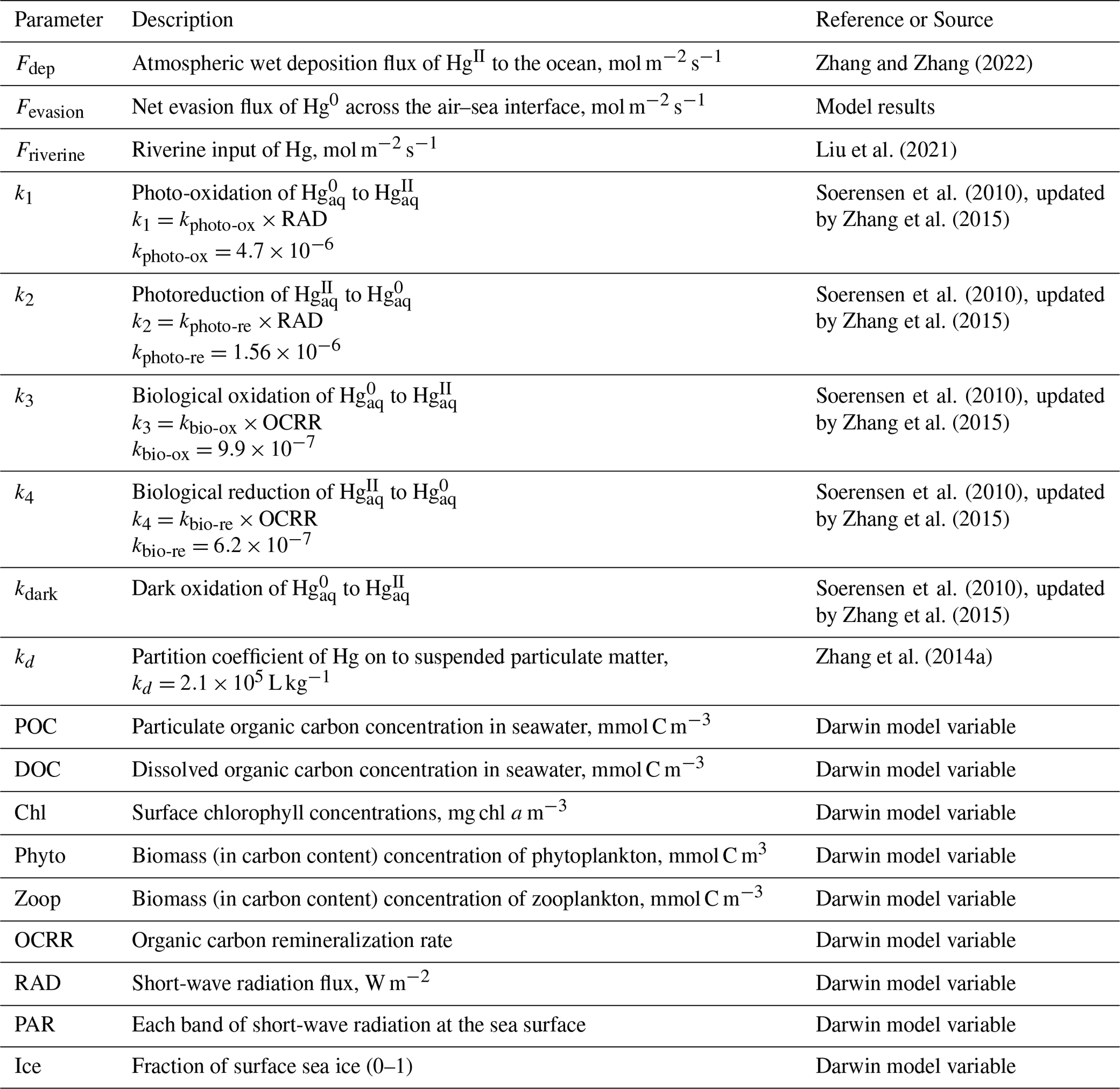
Table 1 Description of the main processes and input fields used in the MITgcm-Hg simulation.

3 Model evaluation

3.1 Global inorganic Hg distribution in surface ocean

The global average daily inorganic Hg (Hg⁰ and Hg²) distribution in surface ocean derived from our high-resolution-MITgcm$/$Hg simulation compares to the observed total Hg concentrations in global surface seawater (Fig. 1). Our model considers the effects of temperature, ocean current motion, turbulent mixing, and nearshore topography, all contributing to differences in oceanic Hg distribution. As a result, we obtain a more refined global distribution of Hg at the ocean surface. Delicate simulations of inorganic Hg in the surface ocean reflect regional differences and eddy scale changes of concentration, which are aroused by ocean currents or geographical factors. Our high-resolution model shows more detailed changes and a clearer gradient between continent and ocean due to the narrower, swifter currents and strong shear, which can increase the efficiency of mixing. Overall, the distribution of inorganic Hg in our model is similar to that simulated in the lower-resolution ECCO v4 MITgcm (Fig. S1 in the Supplement). The modeled concentration of Hg (mean and standard deviation: 0.60 ± 1.41 pM) is slightly lower than the observed concentration (0.87 ± 0.46 pM) in seawater. As we use a similar Hg chemistry and exchange scheme as previous models (Table 1), the difference in model results reflects a potential dependence of these parameters on model resolution. Besides, the various parameters of the ecosystem vary greatly between this study and previous ones (e.g., different community structures, etc.).

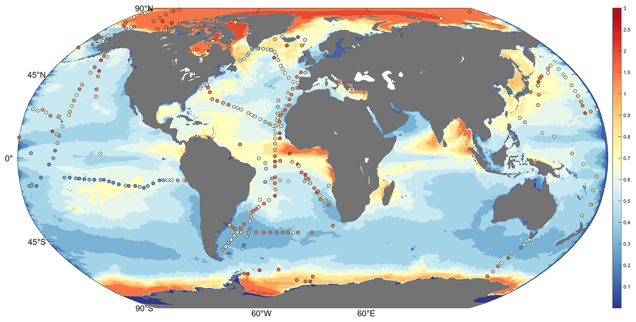
Figure 1 Global simulation of the daily mean total inorganic Hg (0–10 m depth; color, unit pM (10⁻⁹ mol m⁻³)) and observation of total inorganic Hg in the ocean surface (0–10 m depth; scatter, unit pM). Observations are from the North Pacific Ocean (Laurier et al., 2004), the Atlantic (Kuss et al., 2011), the Equator and South Atlantic (Mason and Sullivan, 1999), the North Atlantic (Mason et al., 1998, 2001; Bowman et al., 2015), the Southern Ocean (Cossa et al., 2011), and the Arctic Ocean (Kirk et al., 2008; Chaulk et al., 2011; Lehnherr et al., 2011; Heimbuerger et al., 2015).

The simulated total inorganic Hg shows greater global and regional differences compared to previous models. Variables coupled with online biogeochemistry are involved in the chemical production and consumption of inorganic Hg, resulting in modeled Hg concentrations that better match observations (the Hg^II deposition flux and Hg⁰ evasion flux are shown in Fig. S2). Typically, observations are not continuous, and the values of certain adjacent observations may vary dramatically. This variability has been observed in the high-precision cruise data (Fig. 2 Scattered points in red box). This indicates that the distribution of Hg in the real ocean is highly variable, but this variation was not apparent due to the resolution limits in the previous marine models. Figure 2 illustrates that high-resolution simulated results are closer to observations than previous lower-resolution models (Zhang et al., 2020). In the circled position in the red box, Fig. 2a and c can replicate the apparent difference in the observed data at nearby locations simultaneously (or in a short time).

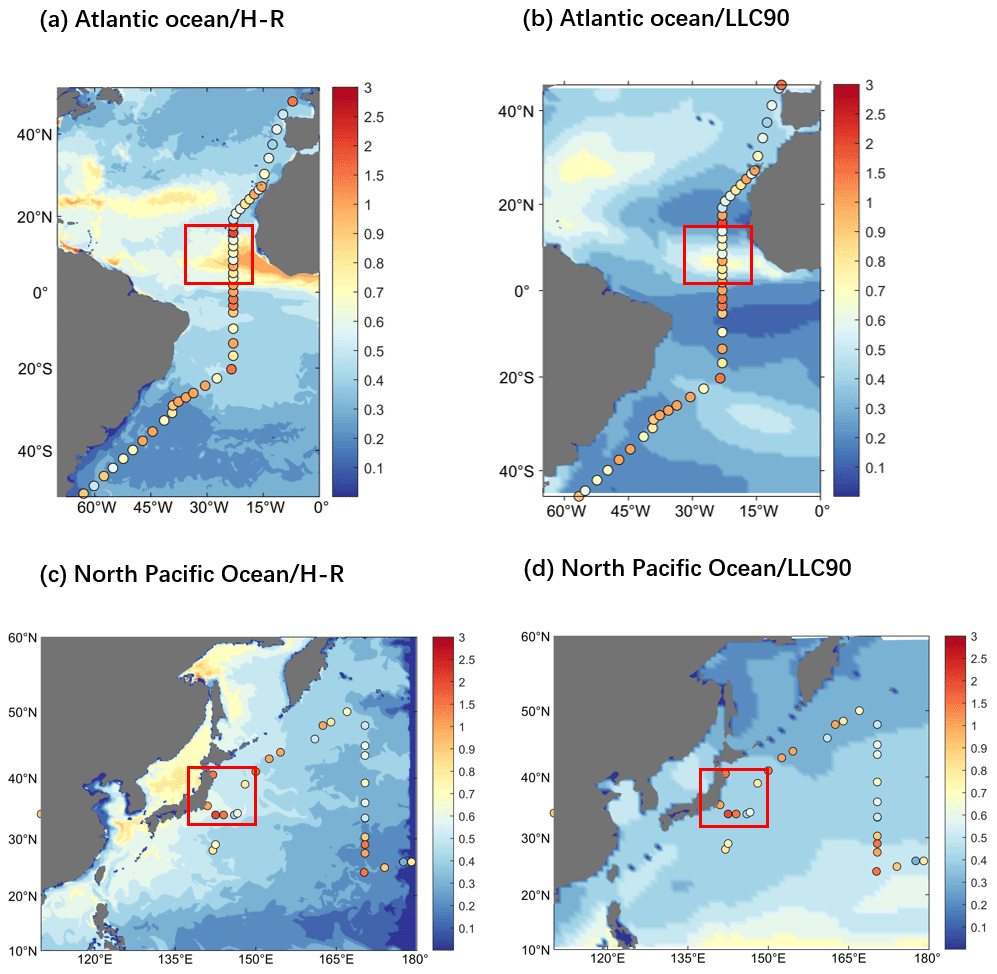
Figure 2 MITgcm simulation for total inorganic Hg results of high-resolution ($\mathrm{1}/\mathrm{5}$^∘ × $\mathrm{1}/\mathrm{5}$^∘ horizontal) ECCO2 (H-R) and coarser-resolution (1^∘ × 1^∘ horizontal) ECCO v4 (LLC90) (0–10 m depth; color, unit pM, Huang and Zhang, 2021). The scatter is observations from two single high spatial precision cruises, (a, b) from Kuss et al. (2011), Atlantic Ocean observations in a month, and (c, d) from Laurier et al. (2004), North Pacific observations in a day (0–10 m depth; scatter, unit pM).

For quantitative descriptions closer to the observation with the high-resolution model (HR) than with the lower-resolution model (LLC90), we calculated the disparity between the observation and the model-simulated results (the values at the position consistent with the observation). We employed two indicators for comparison: firstly, the sum of the absolute between the simulated values and the observation. A smaller value indicates a smaller simulation–observation disparity (simulation is closer). Our findings reveal that for HR, indicator 1 is 23.11 (Fig. 2a) and 10.11 (Fig. 2c), while for LLC90, it is 30.11 (Fig. 2b) and 11.41 (Fig. 2d). Secondly, we used the absolute value of the covariance between the simulated outcomes and the observation. Larger values denote a stronger correlation, indicating a closer alignment between the simulation and observation. Our results indicate that for HR, indicator 2 is 0.012 (Fig. 2a) and 0.010 (Fig. 2c), and for LLC90, it is 0.001 (Fig. 2b) and 0.009 (Fig. 2d). Both of these indicators collectively underscore the quantified closeness of our HR model simulation outcomes to the observed data.

Ocean currents and turbulence play an important role in the physical transport of Hg. Strong upwelling occurs where the western boundary stream is strong or where cold and warm currents meet, which facilitates the horizontal and vertical exchange of Hg in the ocean, resulting in a heterogeneous distribution and in drastic changes. In addition, turbulence across the ocean causes the spread of Hg in a vortical shape. The finer portrayal of inorganic Hg in Fig. 3 demonstrates the influence of ocean currents and turbulence. The Kuroshio in the western Pacific Ocean and the Gulf Stream in the North Atlantic Ocean are the most powerful western boundary currents in the world, and the western boundary flow region has very active vortices and a fast flow rate. This region shows more apparent concentration changes and clear eddy structures in the distribution of inorganic Hg compared to the surrounding ocean (Fig. 3a and b). Other areas in the distribution of Hg with apparent changes are the Pacific and Atlantic equatorial regions, which are possibly influenced by the Westward Equatorial warm currents. Moreover, the transport and mixing of Hg are stronger and faster where cold and warm currents meet (Fig. 3b and d). It was also found that cold currents have a milder effect on Hg transport and dispersion than warmer currents (Fig. 3c and d).

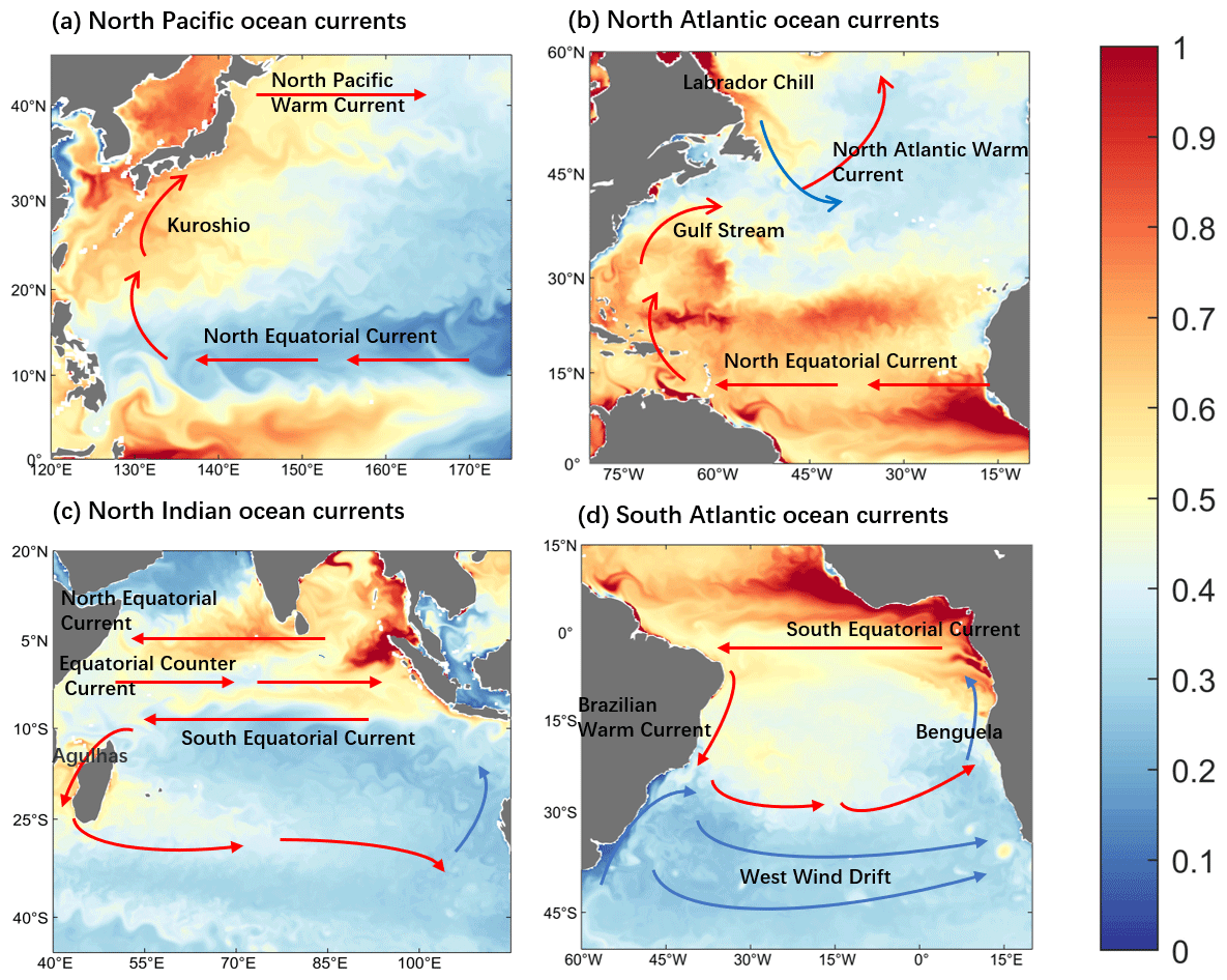
Figure 3 Distribution of inorganic mercury at the sea surface within regions influenced by various global ocean currents (0–10 m depth; color, unit pM). Zoom for (a) the Northwest Pacific Ocean current-affected area, (b) the Northwest Atlantic Ocean current-affected area, (c) the North Indian Ocean current-affected area, and (d) the South Atlantic Ocean current-affected area.

3.2 Riverine Hg discharge

Rivers are important sources of coastal Hg. We model Hg from rivers as a refractory tracer following Zhang et al. (2015), driven by the riverine input (1000 Mg a⁻¹, 893–1224) from Liu et al. (2021). Before using the river discharge as the model input, we interpolated the river discharge so that its spatial resolution is consistent with the HR MITgcm model. After transferring and mixing for 6 months in our simulation (Fig. 4), most of the Hg (93.7 %) is buried in estuarine sediments (ocean depth < 55 m), while 6 % is buried in shelves (ocean depth between 55 and 180 m), with less than 0.01 % export to the open ocean (ocean depth > 180 m). We model a higher percentage of refractory particulate oxidized Hg (HgPR) buried in estuarine sediments and less buried in shelves and exports to the open ocean, compared with previous studies. For example, 72 %–73 % was buried in estuarine sediments and 5 %–6.4 % was transported to the open ocean according to Zhang et al. (2015) and Liu et al. (2021). Indeed, with a higher resolution, coastal currents can be resolved with river discharge being transferred along the seashores. By contrast, the coarse-resolution model assumes even mixing at the first grid point for a long distance, leading to an overestimate of the transmission to distant oceans.

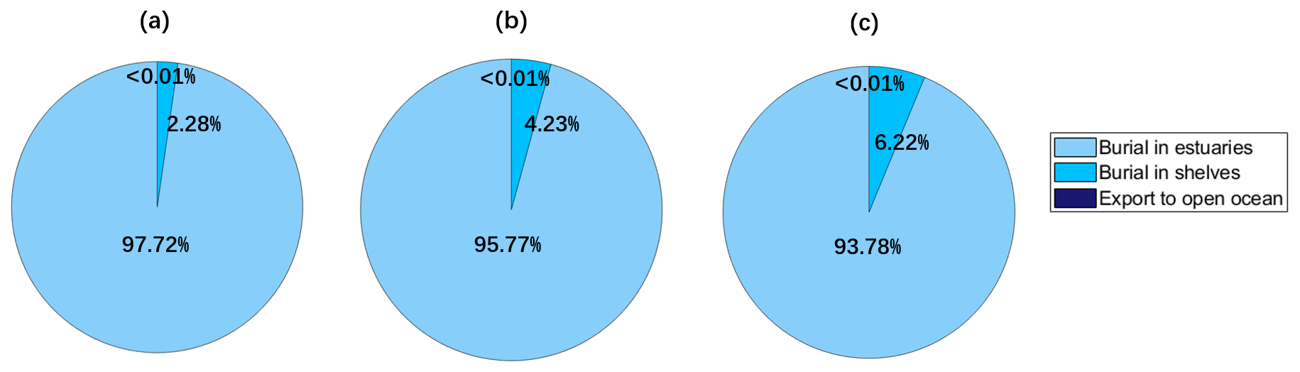
Figure 4 Global simulations of the fate of refractory particulate oxidized Hg (HgPR) discharged by rivers. Estuaries, shelves, and open oceans are defined as ocean regions with depth < 55, 55–185, and > 185 m, respectively. Coastal ocean refers to estuaries and the shelf. (a)–(c) Simulation results of the last day of 4–6 months, respectively.

The spatial distribution of riverine input refractory particulate oxidized Hg across the global ocean is driven by both variabilities in HgPR concentrations and suspended sediment discharges (Fig. 5). Major rivers and highly contaminated systems are visible on the global chart (e.g., Yangtze, Amazon, Ganges). The high Hg discharges from Mexican rivers into the Pacific Ocean reflect the high total suspended sediment flux values, as previously described by Liu et al. (2021). To understand better the fate of HgPR discharge, we zoom in on the major river mouth regions for further investigation. The rivers selected for the analysis include the Rio Grande in North America, the Yellow River, the Yangtze River, the Amur River, the Pearl River, and the Zigzag River in Asia, the Orinoco River and the Amazon River in South America, and the Congo River in Africa. We find that when HgPR is transported from river mouths, it flows along the coast in an eddy shape and in the direction in which the Coriolis force works. However, most of it is buried in estuaries and less is exported to the open ocean. Thus, HgPR has a limited impact on Hg concentrations in surface seawater beyond the shelf region and greatly impacts environmental pollution in coastal and shelf regions. Hg exports from rivers are important to specific coastal areas, and Liu et al. (2021) have raised further concerns about riverine Hg and about a deeper understanding of the role of rivers in the global Hg cycle.

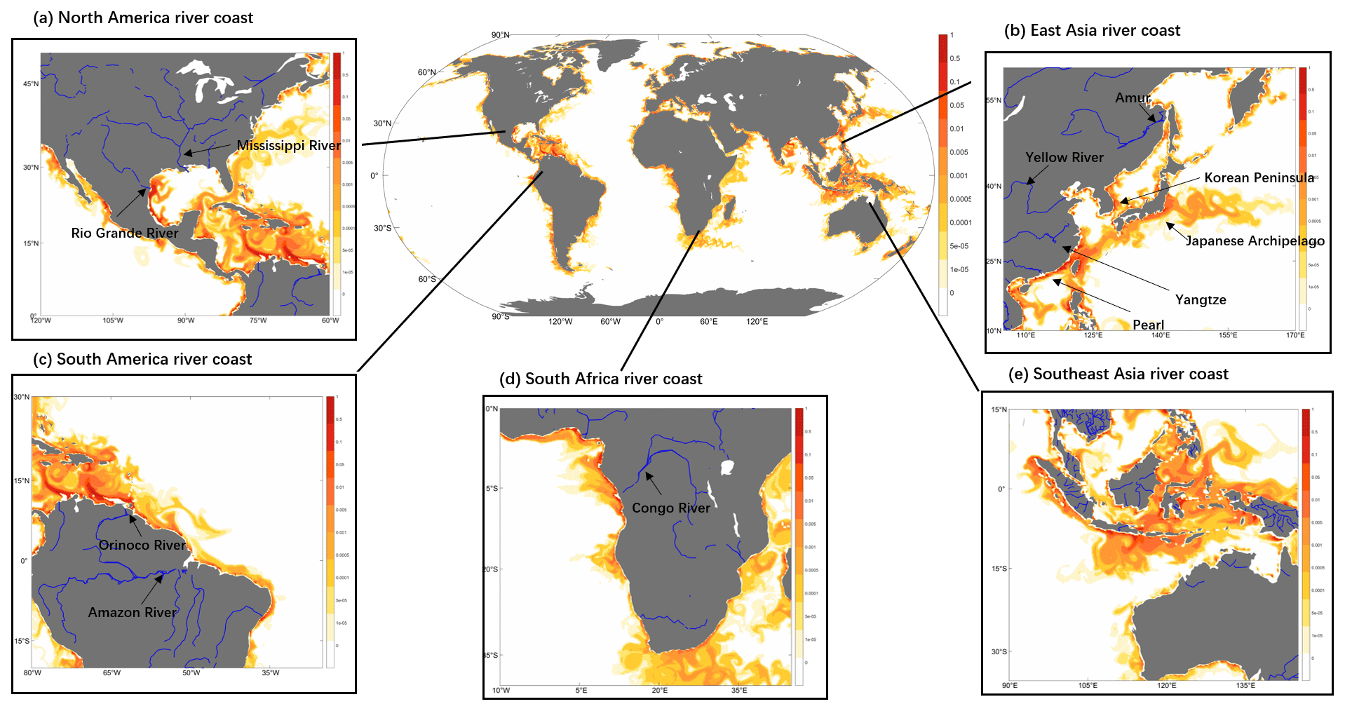
Figure 5 Global and coastal distribution of daily refractory particulate oxidized Hg (HgPR) on the last simulation day (0–10 m depth; color, unit pM). Zoom for (a) North American river coast, (b) East Asia river coast, (c) South American river coast (d) South African river coast, (e) Southeast Asia river coast.

In the case of the Amazon River (Fig. 5c), which is the largest exporter of freshwater and particulate matter to marine waters globally (Amos et al., 2014), generating up to 1.3×10⁶ km² plume and extensive muddy bottoms in the equatorial margin of South America (Moura et al., 2016). Our model results show that Hg discharges from the river are transported northwestward along the Brazilian continental shelf without apparent offshore transport before intersecting the Equatorial Counter Current (Fig. 5c). This is consistent with the model simulation by Zhang et al. (2015), but the plume we simulate is much finer and narrower due to the higher resolution of the model. This is also consistent with the observation (Mason and Sullivan, 1999), which shows that there is an apparent absence of a riverine Hg plume and low total Hg concentrations in the open Equatorial Atlantic Ocean near the Amazon River mouth.

Our model results show that HgPR is transported from the coast to the ocean in an outwardly extending eddy shape, indicating the influence of turbulence mixing and the transmission of ocean eddy energy (Wyrtki et al., 1976). Mesoscale eddies are widely present in the global ocean and dominate the ocean's kinetic energy. They are also involved in energy cascade at different scales (Shang et al., 2013). Clayton et al. (2013) proposed that increasing the resolution of physical models can enhance dispersal rates by narrowing and accelerating boundary currents, resolving swift transports associated with eddy stirring. To better illustrate the dynamic process of the transport and mixing of HgPR, we create global and regional videos using data from the entire simulation period (Figs. S6 and S7). The results show that HgPR spreads outward in an eddy shape, driven by HgPR concentrations and influenced by the kinetic energy transmission by ocean eddies and the mixing of turbulence. Compared with the model results in Fig. 3 by Zhang et al. (2015), the distinct depiction of ocean eddies achieved through our HR models is evident. This notably underscores the pivotal role played by eddy-driven processes and turbulence-induced mixing in the transportation and dispersion of river-derived Hg within coastal and shelf regions.

3.3 Impact of biological pump

The spatial distribution of modeled ${\mathrm{Hg}}_{\mathrm{aq}}^{\mathrm{P}}$ sinking flux (Fig. 6c) follows the distribution of POC out of the euphotic zone (Fig. S3). Globally, the ${\mathrm{Hg}}_{\mathrm{aq}}^{\mathrm{P}}$ sinking flux from the surface (0–10 m) is 1.12 mol a⁻¹. The POC pool encompasses both detritus and living phytoplankton in aquatic food webs. Phytoplankton is known to accumulate Hg from the surrounding aqueous environment and is considered to be the primary entry point for Hg into marine food chains (Pickhardt and Fisher, 2007). The modeled distributions of all phytoplankton and zooplankton biomass in the euphotic zone are shown in Fig. 6a and d, respectively. Moreover, the modeled distributions of phytoplankton and zooplankton are consistent with previous model results and observations (Kuhn et al., 2019; Wu et al., 2020). The distribution of surface chlorophyll concentrations (Fig. 6b) also aligns well with the phytoplankton distribution. The model simulates elevated sinking flux of HgP in high-latitude oceans of the Northern Hemisphere due to enhanced nutrient input from terrestrial erosion, in the equatorial region of the Southern Ocean, and along the west coasts of continents with strong upwelling.

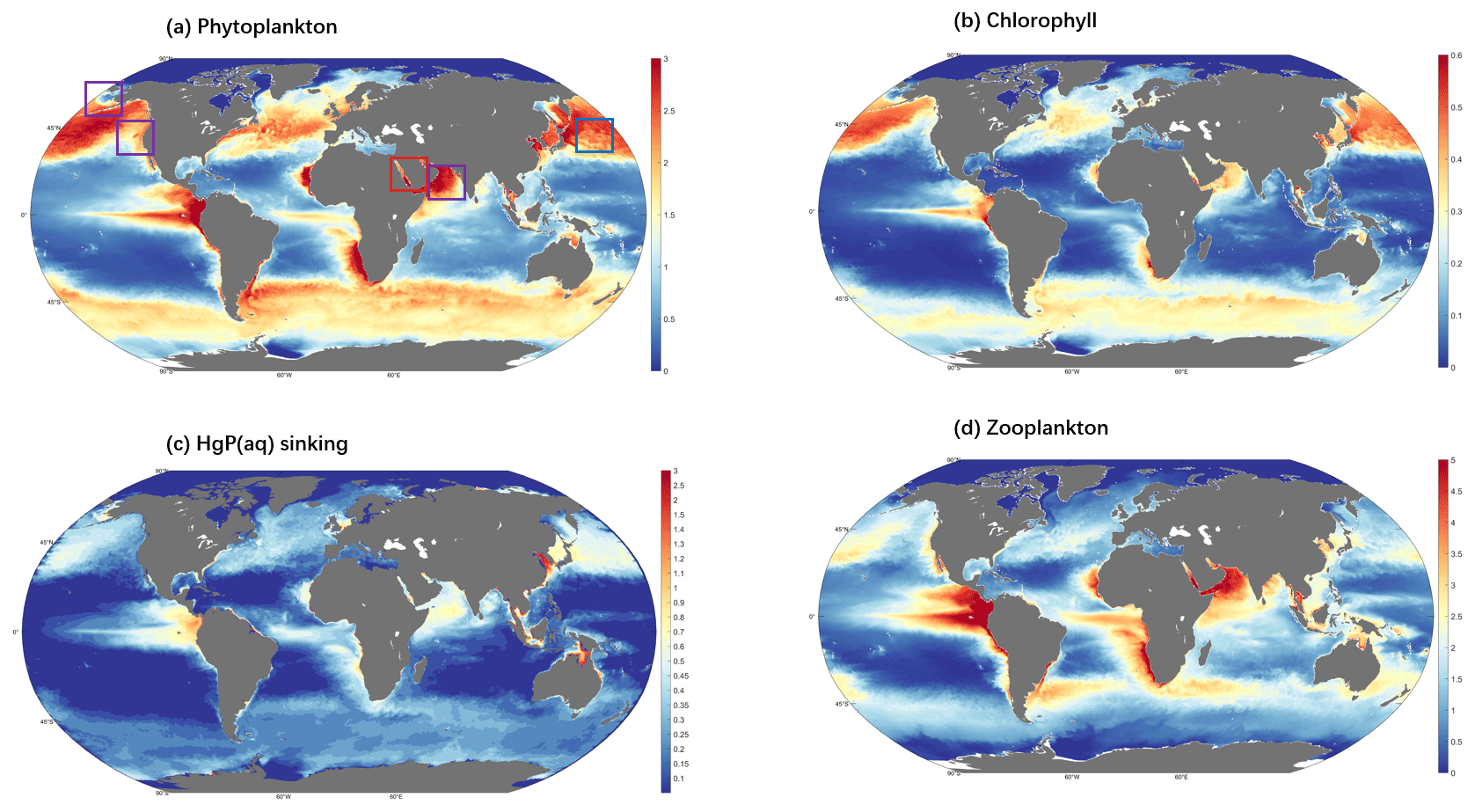
Figure 6 Global distribution of the daily mean ecological variables (0–10 m). (a) The sum of 35 kinds of biomass (in carbon content) concentration of phytoplankton (unit mmol C m⁻³); the areas highlighted by boxes are possible algal regions, and the red box area is the final selected algal region. (b) The sum of 35 kinds of surface chlorophyll concentrations (color, unit mg chl a m⁻³). (c) HgP(aq) sinking flux (color, unit fM (10⁻¹⁵ mol L⁻¹)). (d) The sum of 16 kinds of biomass (in carbon content) concentration of zooplankton, (unit mmol C m⁻³).

Online biogeochemistry makes Hg more sensitive to environmental changes within at least one time step of the model (1 h). In our study, we try to establish a correlation between plankton and the sinking of particle-bound Hg. To achieve this, we need to observe and compare the changes in the HgP sinking flux during periods when plankton undergoes apparent fluctuations. One such process is algal bloom caused by eutrophication. Eutrophication is the process by which the primary production in a water body increases, and in severe cases it can lead to large blooms of algal. Algal bloom mostly occurs in coastal areas: Dai et al. (2023) found that algal blooms occurred in 126 out of the 153 coastal countries examined. These blooms can strongly affect the biogeochemistry in the water column, including the distribution and cycling of nutrients, organic matter, and other elements, as well as Hg. The decomposition of algal debris can increase the flux of particulate organic matter (Macalady et al., 2000) and associated Hg to the sediments. Furthermore, the uptake of Hg by phytoplankton can also increase during algal blooms, leading to higher Hg concentrations in the sinking organic matter. Investigating the changes in the HgP sinking flux during algal blooms can provide valuable insights into the biogeochemical processes controlling the fate and transport of Hg in aquatic systems.

We identify “potential” algal bloom events on a global scale for the simulated period. The International Council for the Exploration of the Sea (ICES) meeting (1984) concluded that a bloom is a deviation from the normal phytoplankton mass. Hence, we can devise an algorithm to identify potential algal bloom events: within the simulated period, an algal bloom event is recognized if it exhibits the most deviation from the average. Certainty regarding the occurrence of a bloom requires additional supporting data, including physicochemical properties of seawater during the same period and remotely sensed imagery demonstrating bloom presence. Nevertheless, our study just aims to exhibit the swift response of Hg behavior in our model to ecosystem changes within a 1 h timeframe. Consequently, an exhaustive validation of an event causing a sudden plankton shift as an algal bloom event is not our primary focus. As a result, the definition of a bloom event in this paper is presented as a potential scenario for modeling, and we have incorporated the qualifier “potentially” into this definition. While this description may not match the precision of an exact bloom event, it does serve to indicate that the biochemical conditions of the ocean are altered when a bloom-like event triggers a surge in phytoplankton.

In this way, we capture five possible bloom regions, located in the Red Sea (detected region's center position: 34.4^∘ E, 26.2^∘ N), the Northwest Pacific (155.5^∘ E, 33.4^∘ N), the Bering Strait (171.2^∘ W, 67.5^∘ N), the West Coast of the United States (124.5^∘ W, 42.2^∘ N), and the southern coast of the Arabian Peninsula (52.2^∘ W, 15.4^∘ N) (Fig. 6a). Upon analyzing the time series data, we observe apparent fluctuations and peaks in the phytoplankton biomass at two regions, Point A in the northwestern Red Sea and Point B in the northwest Pacific Ocean (Fig. 7). To further confirm that these fluctuations are indeed bloom events, we examine the nutrient levels of nitrogen and phosphorus in the water at the two regions (Fig. S4). As elevated nitrogen and phosphorus elements are known to be associated with eutrophication and algal blooms, we find that the nutrient levels at Point A are above the average during the peak days, suggesting the occurrence of algal blooms here. It is possibly attributed to higher sea surface temperature or increased use of nitrogen fertilizers in neighboring countries such as Egypt and Saudi Arabia (Ritchie et al., 2022), both of which can contribute to the blooms (Dai et al., 2023). Previous research has also reported algal bloom events in the Red Sea (Mohamed, 2018). The intense fluctuations in phytoplankton biomass at Point A during the bloom period (possibly between mid-March and early May) are indicative of a bloom event, as shown by the abrupt peaks in plankton biomass, chlorophyll concentration, and ${\mathrm{Hg}}_{\mathrm{aq}}^{\mathrm{P}}$ sinking flux, all of which are significantly higher than the average (Fig. 7).

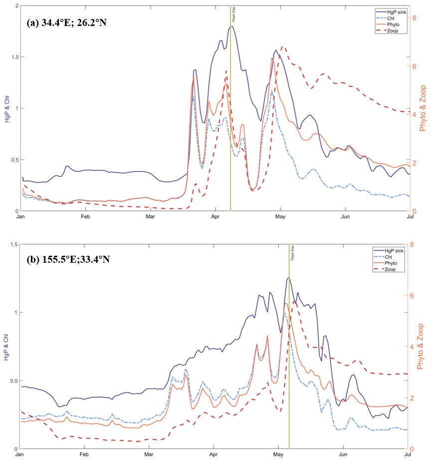
Figure 7 Time-series of HgP(aq) sinking flux (fM m⁻² s⁻¹), the sum of 35 kinds of surface chlorophyll concentrations (mg chl a m⁻³), the sum of 35 kinds of biomass concentration of phytoplankton and zooplankton (mmol C m⁻³) at area of potential algal bloom: (a) Point A in the northwestern Red Sea with Peak day is 7 April and (b) Point B in the northwest Pacific Ocean with Peak Day is 5 May.

We determine the approximate extent of blooms by generating a global distribution of plankton, chlorophyll, and ${\mathrm{Hg}}_{\mathrm{aq}}^{\mathrm{P}}$ sinking flux on the peak day (Fig. S5). Our results indicate that the Point A bloom spanned two latitudes and two longitudes, possibly influenced by coastal topography. On the peak day of Point A bloom, the ${\mathrm{Hg}}_{\mathrm{aq}}^{\mathrm{P}}$ sinking flux is 2.7 times greater than the overall average and 5.2 times greater than the non-blooming mean. This suggests that ecological changes in seawater influence the sinking of particle-bound Hg. During algal blooms, the increased phytoplankton biomass creates more particulate matter to bind with Hg, leading to accelerated organic particle scavenging and remineralization in the water column. Thus, in this way, increases the sinking flux of particle-bound Hg after a short time. Our discovery was facilitated by integrating our model with online biogeochemistry, which promptly reflected the abrupt fluctuations in phytoplankton and enabled us to observe changes in the sinking of Hg particles quickly.

4 Conclusions

In this study, we estimate the global biogeochemical cycling of Hg in a state-of-the-art physical-ecosystem ocean model (high-resolution (HR) MITgcm$/$Hg), realizing Hg transport at eddy scale. One of the biggest advantages of our model is the promoted resolution so that the small-scale changes of marine Hg can be captured. We use the online biogeochemistry fields to participate in the ocean transformation and reaction processes of Hg. Online biogeochemistry is involved in the reaction between elemental Hg and divalent Hg, and the process of particle-Hg forming as well as the remineralization processes. The coupling with the Darwin Project further enhances the specificity of the Hg biogeochemistry in the MITgcm model. Overall, this approach provides a comprehensive understanding of the global biogeochemical cycling of Hg and its interactions with the marine ecosystem.

The horizontal resolution of 18 km allows our model to simulate turbulence, which is omitted in previous global models. Turbulent mixing and shear effects affect the transport of materials (including Hg) in the ocean, and thus only a high enough resolution can refine this physical process. With this advanced physical configuration, we introduce the latest river discharge inventory from Liu et al. (2021) and 12 nutrients exported by river from WaterSheds 2 (Mayorga et al., 2010). Our HR model provides a more detailed depiction of the fate of riverine Hg discharged to the global oceans.

The ocean plays a critical role in the global Hg cycle, and the large size of the ocean is a major site for atmospheric Hg transport, transformation, and deposition. Global ocean models of Hg require a better understanding of biogeochemical controls on Hg speciation. We qualitatively analyzed the biogeochemistry effect on the particle scavenging process of inorganic Hg. The HR MITgcm can help us better predict the transport and fate of Hg in the ocean and its impact on the global Hg cycle. This provides us with more advanced tools and methods to address natural- and human-disturbing global Hg.

The physical transport and biogeochemical changes of Hg in the ocean are complex and have been the subject of prolonged study. However, our HR model optimizes this simulation by capturing the small- to medium-scale dynamics of Hg processes in the ocean, simulating mixed turbulence effects in the nearshore and estuaries. Our improved simulation of biogeochemical conditions also makes it possible to provide help in the rapid response to ecological changes in Hg. Nevertheless, our model does have its limitations. Firstly, HR models with short time steps encounter challenges in comprehensively depicting climate-scale changes. It is difficult to simulate climate change-induced alterations in the oceanic Hg cycle. Secondly, closer integration with ecological models is necessary to characterize processes occurring at finer time scales, including migrations and changes in the structure of phytoplankton communities and the weakening or enhancement of biological pumps. Our coupled HR model with advanced biogeochemistry holds promise in offering fresh insights into the methylation and demethylation processes of Hg. This aspect will be delved into further in our upcoming work. Additionally, we anticipate refining existing models to address a broader range of issues beyond those previously mentioned.