SedTrace 1.0: a Julia-based framework for generating and running reactive-transport models of marine sediment diagenesis specializing in trace elements and isotopes

Trace elements and isotopes (TEIs) are important tools in studying ocean biogeochemistry. Understanding their modern ocean budgets and using their sedimentary records to reconstruct paleoceanographic conditions require a mechanistic understanding of the diagenesis of TEIs, yet the lack of appropriate modeling tools has limited our ability to perform such research. Here I introduce SedTrace, a modeling framework that can be used to generate reactive-transport code for modeling marine sediment diagenesis and assist model simulation using advanced numerical tools in Julia. SedTrace enables mechanistic TEI modeling by providing flexible tools for pH and speciation modeling, which are essential in studying TEI diagenesis. SedTrace is designed to solve one particular challenge facing users of diagenetic models: existing models are usually case-specific and not easily adaptable for new problems such that the user has to choose between modifying published code and writing their own code, both of which demand strong coding skills. To lower this barrier, SedTrace can generate diagenetic models only requiring the user to supply Excel spreadsheets containing necessary model information. The resulting code is clearly structured and readable, and it is integrated with Julia's differential equation solving ecosystems, utilizing tools such as automatic differentiation, sparse numerical methods, Newton–Krylov solvers and preconditioners. This allows efficient solution of large systems of stiff diagenetic equations. I demonstrate the capacity of SedTrace using case studies of modeling the diagenesis of pH as well as radiogenic and stable isotopes of TEIs.

1 Introduction

Trace elements and isotopes (TEIs) play critical roles in the heathy functioning of the marine ecosystem (SCOR Working Group, 2007). For example, Fe, Zn, Ni and other transition metals serve as cofactors in metalloenzymes that are essential for phytoplankton physiology such that the low concentrations of these metals can limit phytoplankton productivity with implications for the global carbon cycle (Martin et al., 1987; Vance et al., 2017; Tagliabue et al., 2017; Morel et al., 2020; Lemaitre et al., 2022). TEIs are also powerful tracers of geological, physical and biogeochemical processes in the ocean (Lam and Anderson, 2018). For instance, the radiogenic isotope of Nd has been used to study ocean circulation and the role of continental weathering and tectonics in past climate changes (Piepgras et al., 1979; Palmer and Elderfield, 1985; Frank, 2002; Goldstein and Hemming, 2003; Du et al., 2020); the stable isotopes of Mo have been used to study past ocean oxygenation (Archer and Vance, 2008; Anbar and Rouxel, 2007; Lyons et al., 2009). Since the dawn of the international GEOTRACES program, there have been increasing efforts aimed at characterizing the distributions, global oceanic budgets, internal cycling and external sources of TEIs in the modern ocean and their utility in paleoceanography (Anderson, 2020; Schlitzer et al., 2018).

In recently years, however, two issues have emerged as major challenges to the understanding and application of marine TEIs. First, the modern oceanic budgets of many TEIs, such as Fe, Cu, Ni, Zn and Nd, cannot be balanced by known sources at the riverine, atmospheric and hydrothermal interfaces, and increasing evidence suggests that fluxes across the sediment–water interface (SWI) may play important, if not dominant, roles in setting the global oceanic budgets of TEIs (Homoky et al., 2016; Jeandel, 2016; Little et al., 2014; Du et al., 2020; Haley et al., 2017; Elrod et al., 2004; Cameron and Vance, 2014; Little et al., 2020). Second, applying TEIs as proxies to study the geological evolution of the ocean system is hampered by the lack of quantitative knowledge of the sedimentary cycling of TEIs, which may alter or completely erase the original proxy signals preserved in sedimentary archives (Horner et al., 2021; Crusius and Thomson, 2000). Models of the sedimentary cycling of TEIs are thus needed to resolve these issues. Quantitative modeling is particularly indispensable in this case because the complexity, heterogeneity, and highly coupled nature of biogeochemical and physical processes in marine sediments make straightforward interpretation of measured modern and paleo-TEI data difficult. In addition, TEI data in sediment pore water are extremely scarce because of analytical and sampling challenges. I thus hope that models can assist our understanding of the sedimentary TEI cycling in the presence of large data gaps.

A diagenetic model is typically a 1-D reactive-transport model that includes physical transport and biogeochemical reactions to simulate the distributions of dissolved substances in pore water and solid substances in sediments (Berner, 1980; Boudreau, 1997; Burdige, 2006). Such models have traditionally been used to study the sedimentary cycling of carbon, oxygen and nutrients (Wang and Van Cappellen, 1996; Boudreau, 1996; Meysman et al., 2003; Soetaert et al., 1996), as well as to a limited extent TEIs like Fe, Mn and U (Dale et al., 2015; Burdige, 1993; Lau et al., 2020; Maher et al., 2006). However, to date there has been little concerted effort to develop diagenetic models specifically for TEIs due to some particular challenges of TEI biogeochemistry. First, a realistic digenetic TEI model needs to include a pH module to enable speciation modeling. Pore water pH is difficult to model because of the large network of biogeochemical and physical processes involved (Boudreau and Canfield, 1988, 1993; Jourabchi et al., 2008; Reimers et al., 1996). Many studies thus ignore TEI speciation in diagenetic models. Moreover, TEIs are commonly influenced by more biogeochemical reactions than the major and minor constituents. Together with the necessity for pH and speciation modeling, a diagenetic model may need to include a large system of differential equations that are also highly stiff because the span of the reaction timescales can be large (Boudreau, 1997). Thus, unlike traditional diagenetic models of carbon, oxygen and nutrients, diagenetic TEI models also need to take into account numerical efficiency, especially if the goal is to couple diagenetic models to global ocean biogeochemical models (Hülse et al., 2018; Archer et al., 2002).

The greatest challenge from the user's point of view is that most diagenetic models are too specialized to be adaptable. The strong heterogeneity of marine sediments implies that no single diagenetic model can be created to include all sedimentary processes applicable to all environmental settings (Paraska et al., 2014). Often, modelers create specific diagenetic models with fixed selection of substances and processes for their own studies. The model code is often not open-source, and it could be time-consuming and error-prone for other users to adapt the code for new studies. Writing and modifying code require strong programming skills, which is a significant hurdle to the general user. Thus, rather than creating one all-encompassing diagenetic model, it is preferable to create a modeling framework that can generate custom models, allowing users with limited programming skills to create and run models satisfying their own needs (Soetaert and Meysman, 2012).

In this study, I describe SedTrace 1.0, a modeling framework that automates the generation of Julia code for diagenetic models and provides high-performance computing tools to assist model simulation, only requiring the user to supply information using a Microsoft Excel input file. SedTrace specializes in modeling TEIs and can accommodate a wide range of custom pH and speciation modeling choices. The design principle is to give as much control to the user as possible when generating the model such that SedTrace is only meant to help convert user ideas to code rather than make model decisions for the user. Julia is an open-source, dynamically typed programming language for high-performance scientific computing (Bezanson et al., 2017). It offers the high productivity of scripting languages like Python, but can also match the performance of statically typed languages such as C and FORTRAN. It is increasingly being adopted by the climate and ocean modeling community (Pasquier et al., 2022; Sridhar et al., 2022; Sulpis et al., 2022), with well-supported ecosystems relevant to solving differential equations (Rackauckas and Nie, 2017).

This paper is structured as follows. First I describe the model equations and framework in Sect. 2. I then discuss the code generation procedure for physical processes and biogeochemical reactions in Sects. 3 to 5. The numerical solution of the model is discussed in Sects. 6 and 7. Finally, I present a few case studies in Sect. 8 and briefly touch on future development in Sect. 9.

2 Model framework

SedTrace uses the 1-D diagenetic equation (Boudreau, 1997; Meysman et al., 2003):

$$\begin{array}{}\text{(1)}& {\displaystyle \frac{\partial }{\partial t}}{\mathit{\varphi }}^{\mathit{\xi }}{C}_i^{\mathit{\xi }}+T_i={\mathit{\varphi }}^{\mathit{\xi }}{R}_i,\text{(2)}& {\displaystyle }{T}_i={\displaystyle \frac{\partial }{\partial x}}{F}_i^{\mathit{\xi },\mathrm{adv}}+{\displaystyle \frac{\partial }{\partial x}}{F}_i^{\mathit{\xi },\mathrm{diff}}+{\mathit{\varphi }}^{\mathit{\xi }}{T}_i^{\mathrm{bio}},\end{array}$$

where $C_i^{\mathit{\xi }}$ is the concentration of model substance i in the phase ξ (f for pore water or s for solid sediment), ϕ^ξ is the phase volume fraction, T_i is the transport due to advection, diffusion and bio-irrigation, R_i is the net source or sink due to biogeochemical reactions, t is time, and x is the sediment depth coordinate staring from the SWI pointing downward. In SedTrace, the default units are millimoles (mmol) for mass, years for time and centimeters (cm) for length. For example, reaction rates are in units of millimoles per cubic centimeter per year (mmol cm⁻³ yr⁻¹).

The transport terms have well-established forms in diagenetic models (Berner, 1980; Boudreau, 1997). It is largely the reaction terms which are case-specific that create the diversity of diagenetic models and thus cause their poor adaptability. SedTrace fixes the general forms of the transport terms and only requires users to supply case-specific parameters, while letting the user set the reaction terms freely.

Using user-specified spatial grids, which can be nonuniform, SedTrace discretizes Eq. (1) using the method of lines in the time dimension and finite-volume method in the space dimension (Boudreau, 1996), resulting in a system of ordinary different equations (ODEs) of time only:

$$\begin{array}{}\text{(3)}& \begin{array}{rl}{\displaystyle \frac{\mathrm{d}}{\mathrm{d}t}}{C}_{i,j}^{\mathit{\xi }}& ={\displaystyle \frac{F_{i,j-\frac{\mathrm{1}}{\mathrm{2}}}^{\mathit{\xi },\mathrm{adv}}-F_{i,j+\frac{\mathrm{1}}{\mathrm{2}}}^{\mathit{\xi },\mathrm{adv}}}{{\mathit{\varphi }}_j^{\mathit{\xi }}\mathrm{\Delta }{x}_j}}+{\displaystyle \frac{F_{i,j-\frac{\mathrm{1}}{\mathrm{2}}}^{\mathit{\xi },\mathrm{diff}}-F_{i,j+\frac{\mathrm{1}}{\mathrm{2}}}^{\mathit{\xi },\mathrm{diff}}}{{\mathit{\varphi }}_j^{\mathit{\xi }}\mathrm{\Delta }{x}_j}}\\ & +R_{i,j}-T_{i,j}^{\mathrm{bio}},\end{array}\end{array}$$

where j is the index of the grid cell. $F_{i,j-\frac{\mathrm{1}}{\mathrm{2}}}^{\mathit{\xi }}$ and $F_{i,j+\frac{\mathrm{1}}{\mathrm{2}}}^{\mathit{\xi }}$ are the fluxes across the left and right boundaries of the cell, respectively. Δx_j is the volume of the cell.

The diffusive and advective fluxes are discretized using the finite-volume–complete flux (FV-CF) scheme (Llorente et al., 2020; ten Thije Boonkkamp and Anthonissen, 2010, 2011). The finite-volume method is preferred in diagenetic models because it ensures mass conservation, whereas the finite-difference method may not.

The finite-volume flux $F_{i,j+\frac{\mathrm{1}}{\mathrm{2}}}^{\mathit{\xi }}$ is derived based on the analytical solution of the local two-point boundary value problems and is partitioned into a homogeneous flux and an inhomogeneous flux. Presently SedTrace only uses the homogeneous flux term. The symbolic derivation of these fluxes using Mathematica can be found in /math/fvcf.pdf.

The resulting discretization may be viewed as a weighted average of the centered scheme and the upwind scheme, and the weight is controlled by the cell Péclet number $\frac{v^{\mathit{\xi }}\mathrm{\Delta }x}{\mathrm{2}{D}^{\mathit{\xi }}}$, where v^ξ is the advective velocity and D^ξ is the diffusion coefficient. At high Péclet numbers (advection dominant), the scheme approaches the upwind scheme, while at low Péclet numbers (diffusion dominant) it approximates the centered scheme. This ensures at least first-order uniform convergence regardless of the Péclet number. Similar Péclet-number-dependent schemes have been applied to diagenetic and ocean modeling (Fiadeiro and Veronis, 1977; Soetaert and Meysman, 2012; Boudreau, 1996). The numerical diffusion introduced in advection-dominated cases has a greater impact on transient than steady-state simulations (ten Thije Boonkkamp and Anthonissen, 2011, 2010). Thus, SedTrace 1.0 is best suited for steady-state modeling of tracer profiles in sediments rather than transient simulations of paleo-proxy evolution.

SedTrace collects the discretized model substances into an MN vector:

$$\begin{array}{}\text{(4)}& \mathit{C}=[C_{\mathrm{1},\mathrm{1}}{C}_{\mathrm{2},\mathrm{1}}\mathrm{\dots },C_{M,\mathrm{1}},\mathrm{\dots },C_{i,j},\mathrm{\dots },C_{\mathrm{1},N}{C}_{\mathrm{2},N},\mathrm{\dots }{C}_{M,N}],\end{array}$$

where M is the number of model substances and N is the number of grid cells. The system of ODEs including boundary conditions can be written in the matrix form:

$$\begin{array}{}\text{(5)}& {\displaystyle \frac{\mathrm{d}}{\mathrm{d}t}}\mathit{C}=\mathbf{A}\mathit{C}+\mathbf{B}\mathit{C}+\mathit{b}+\mathit{S}.\end{array}$$

A is an MN×MN matrix including the linear diffusion and advection operators. B is an MN×MN matrix containing the homogeneous part of the boundary conditions. b is an MN vector containing the nonhomogeneous part of the boundary conditions. S is an MN vector, generally a nonlinear function of C, incorporating the reaction and bio-irrigation sources and sinks, as well as nonlinear coupling of transport.

To generate code for Eq. (5) the user supplies an Excel file model_config.xlsx to SedTrace. An example of a simple Fe cycle model (SimpleFe) can be found in /examples/SimpleFe/model_config_simpleFe .xlsx, and the spreadsheets are shown in Tables 1 to 7. The substances sheet (Table 1) lists the modeled substances, their types (e.g., solid or dissolved), chemical formula and boundary conditions. The reactions sheet (Table 2) lists the kinetic reactions, their chemical equations and rate expressions. The speciation sheet (Table 3) lists aqueous speciation reactions. The adsorption sheet (Table 4) lists the adsorbed species. The diffusion sheet (Table 5) lists information to compute the diffusion coefficients of dissolved substances. The parameters sheet (Table 6) lists the parameters required by the model. The output sheet (Table 7) is used to formulate output and plotting. The data sheet (not shown here) includes observational data that will be plotted together with model outputs.

The workflow of generating and running diagenetic models using SedTrace is shown in Fig. 1. In Sects. 3 and 4, I will describe the mathematical formulation of each of the terms in Eqs. (1), (2) and (5), as well as how SedTrace generates the corresponding code. I will use SimpleFe to illustrate this process. In this paper, I use monospaced font to indicate computer code; variable names in the code, Excel spreadsheet and column names; and Julia file names.

Figure 1 SedTrace framework and workflow.

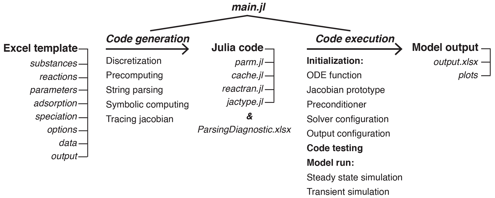
Table 1 The substances sheet of the SimpleFe model.

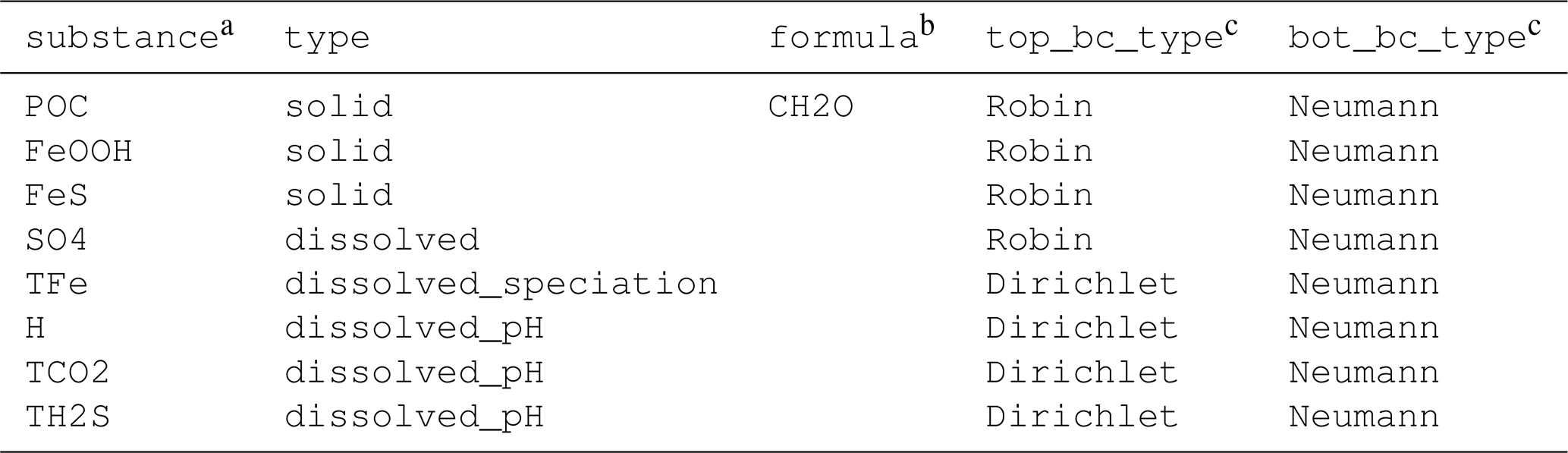
^a Code name for the model substance. ^b Chemical formula that can be used to write chemically balanced equations in the reactions sheet. ^c For model substances of type dissolved_speciation, the boundary conditions listed here are for the total dissolved concentration.

Table 2 The reactions sheet of the SimpleFe model.

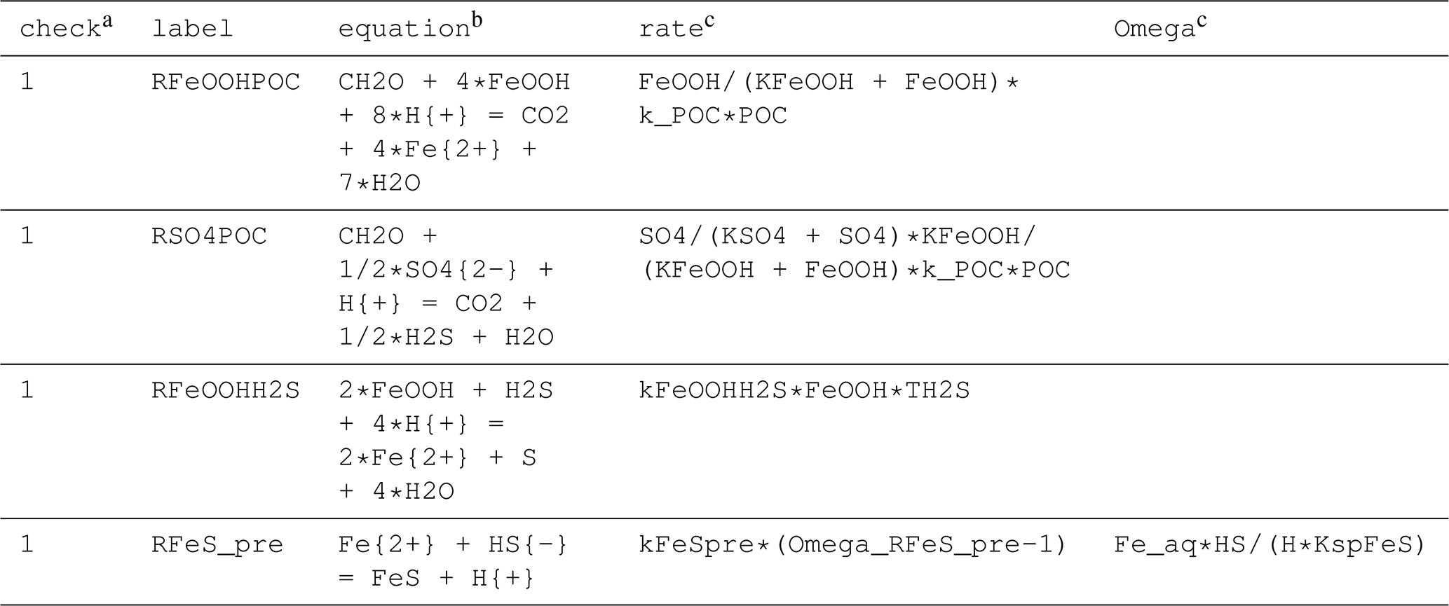
^a Chemical balance is checked if check is set to 1. ^b Equations can be written using the code name or the chemical formula of model substances or the code names and formulae of their dissolved and adsorbed species. ^c Rate and omega expressions can be written only using the code name of the model substances or the code names of their dissolved and adsorbed species.

Table 3 The speciation sheet of the SimpleFe model.

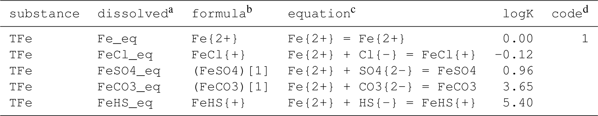
^a Code name of the dissolved species; it must be different from the names of model substances in the substances sheet. ^b Chemical formula that can be used to write the chemical equations; it must be different from the formulae of model substances in the substances sheet. ^c Equations should be written using the formula, not code name. ^d Set to 1 if the concentration of the species is required.

Table 4 The adsorption sheet of the SimpleFe model.

^a Code name of dissolved species that appears in the speciation sheet or the code name of the total dissolved concentration. ^b Code name of adsorbed species. ^c Surface to be adsorbed onto; it can be either the code name of a solid substance from the substances sheet or left empty. ^d Expression can be written only using the code names of the dissolved and adsorbed species listed in the same row; adsorption parameters need to be supplied to the parameters sheet. ^e The boundary conditions of the adsorbed species, which should be the same for all adsorbed species of the same substance.

Table 5 The diffusion sheet of the SimpleFe model.

^a Code name of the dissolved model substance or its total dissolved concentration. ^b The corresponding name listed in SedTrace's database of the diffusion coefficients.

Table 6 The parameters sheet of the SimpleFe model. A template of this sheet can be generated using generate_parameter_template().

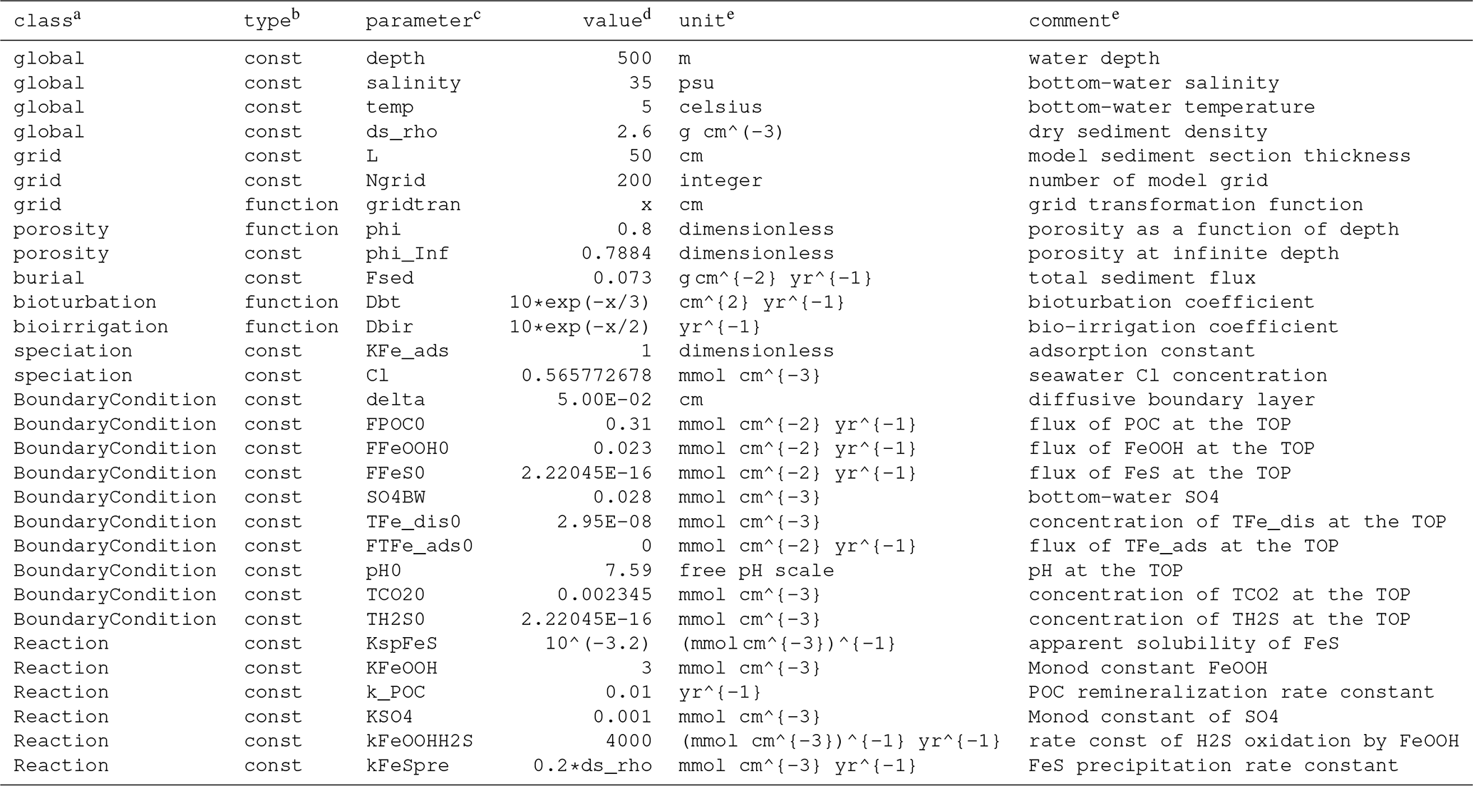
^a Class must be specified using one of the key words shown here following the same order. ^b Type can be constant or a function of depth x. ^c Code name for parameters. ^d To enter the value for the parameter, either supply a numerical value, a function of depth, or a string expression that computes the value using other parameters, in which case the parameters being depended on must appear earlier in the table. The values shown here for the SimpleFe model are only for illustration. ^e Optional.

Table 7 The output sheet of the SimpleFe model.

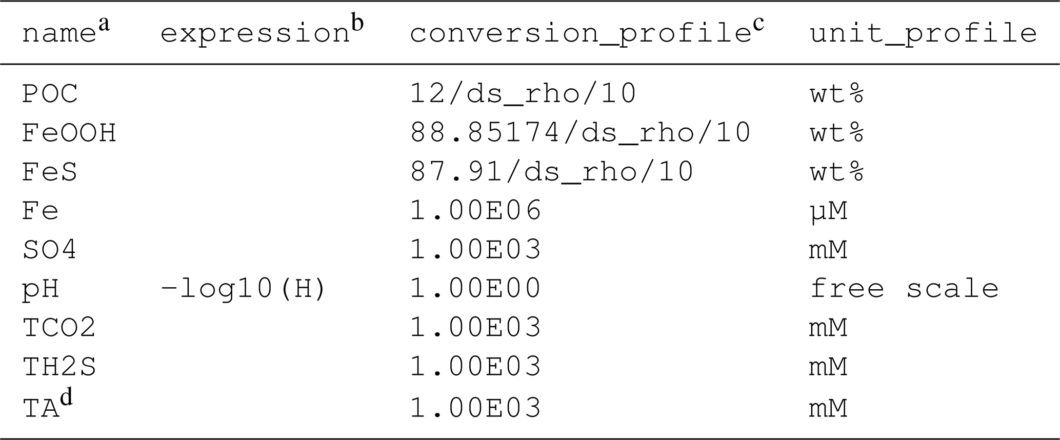
^a Code name for output variables; this can be the same as the model substances or new variable names. ^b Expressions to compute new variables if needed; the expression can use model parameters listed in parm.jl. ^c Multiplication factors that convert default SedTrace units to custom units in unit_profile; these can use model parameters listed in parm.jl – must not be empty (use 1 instead). ^d TA is computed internally and does not need an expression.

3 Grid, transport and boundary conditions

3.1 Grid

To generate the model grid, the user specifies the number of grids (Ngrid), the length of the sediment domain (L) and a grid transformation function (gridtran) in the parameters sheet. SedTrace internally creates a uniform grid between 0 and L cm and uses gridtran to transform it to the user-desired grid (using function x->x will preserve the original uniform grid). A nonuniform grid is used to reduce numerical error at locations where finer spacing is needed (Meysman et al., 2003): for example, close to the SWI where biogeochemical gradients are often the sharpest. SedTrace allows the user to supply parameters as constants or functions of depth x, as labeled in the type column of the parameters sheet (Table 6): for example, gridtran as a function in this case. SedTrace will convert the function string to Julia function and use broadcast() to vectorize the function if necessary. The generated model grid code for SimpleFe using a gridtran that has small grid spacing closer to the SWI is as follows.
#---------------------------------
# grid parameters
#---------------------------------
L = 50.0 # cm # model sediment section thickness
Ngrid = 200 # integer # number of model grid
ξ = range(0, step = L / (Ngrid), length = Ngrid + 1)
# cm # uniform grid
xv = broadcast(x -> L * (exp(x / 5) - 1) / (exp(L / 5) - 1), ξ) # cm # non-uniform grid transformation
x = (xv[2:(Ngrid + 1)] . +xv[1:Ngrid]) / 2 # cm # cell center
dx = xv[2:(Ngrid+1)] .- xv[1:Ngrid] # cm # cell volume

3.2 Advection

The advective flux in Eq. (2) is

$$\begin{array}{}\text{(6)}& F_i^{\mathit{\xi },\mathrm{adv}}={\mathit{\varphi }}^{\mathit{\xi }}{v}^{\mathit{\xi }}{C}_i^{\mathit{\xi }},\end{array}$$

where v^ξ is the phase velocity. To calculate v^ξ, SedTrace makes two assumptions (Boudreau, 1997; Meysman et al., 2003; Berner, 1980): sediment compaction is at steady state and therefore the volume fractions of fluid ϕ^f and solid ${\mathit{\varphi }}^{\mathrm{s}}\left(=\mathrm{1}-{\mathit{\varphi }}^{\mathrm{f}}\right)$ are functions of depth but not time, and the final burial velocities of fluid and solid are the same, $v_{\mathrm{\infty }}^{\mathrm{f}}=v_{\mathrm{\infty }}^{\mathrm{s}}$, without externally forced pore water advection. Using the user-supplied porosity function ϕ^f (phif), porosity at burial depth ${\mathit{\varphi }}_{\mathrm{\infty }}^{\mathrm{f}}$ (phif_Inf), density of dry sediments ρ^s (ds_rho) and solid burial flux $F_{\mathrm{total}}^{\mathrm{s}}$ (Fsed) in parameters, SedTrace computes the phase velocities:

$$\begin{array}{}\text{(7)}& {\displaystyle }{v}_{\mathrm{\infty }}^{\mathrm{s}}={\displaystyle \frac{F_{\mathrm{total}}^{\mathrm{s}}}{{\mathit{\rho }}^{\mathrm{s}}(\mathrm{1}-{\mathit{\varphi }}_{\mathrm{\infty }}^{\mathrm{f}})}},\text{(8)}& {\displaystyle }{v}^{\mathrm{f}}\left(x\right)={\displaystyle \frac{{\mathit{\varphi }}_{\mathrm{\infty }}^{\mathrm{f}}{v}_{\mathrm{\infty }}^{\mathrm{s}}}{{\mathit{\varphi }}^{\mathrm{f}}\left(x\right)}},\text{(9)}& {\displaystyle }{v}^{\mathrm{s}}\left(x\right)={\displaystyle \frac{(\mathrm{1}-{\mathit{\varphi }}_{\mathrm{\infty }}^{\mathrm{f}})v_{\mathrm{\infty }}^{\mathrm{s}}}{\mathrm{1}-{\mathit{\varphi }}^{\mathrm{f}}\left(x\right)}}.\end{array}$$

In SimpleFe the resulting code is as follows.
#--------------------------------------
# porosity parameters
#--------------------------------------
phi_Inf = 0.7884 # dimensionless # porosity at infinite depth
phif = broadcast(x -> 0.8 + (0.9 - 0.8) * exp(-x / 2), x) # dimensionless # fluid volume fraction
phis = 1.0 .- phif # dimensionless # solid volume fraction
#--------------------------------------
# phase velocity parameters
#--------------------------------------
Fsed = 0.073 # g cm^-2 yr^-1 # total sediment flux
w_Inf = Fsed / ds_rho / (1 - phi_Inf) # cm yr^-1 # solid sediment burial velocity at infinite depth
uf = phi_Inf * w_Inf ./ phif # cm yr^-1 # pore water burial velocity
us = Fsed / ds_rho ./ phis # cm yr^-1 # solid sediment burial velocity

3.3 Diffusion

For solid substances SedTrace considers the diffusive flux due to bioturbation (Boudreau, 1997):

$$\begin{array}{}\text{(10)}& F_i^{\mathrm{s},\mathrm{diff}}=-{\mathit{\varphi }}^{\mathrm{s}}{D}^{\mathrm{b}}{\displaystyle \frac{\partial C_i^{\mathrm{s}}}{\partial x}},\end{array}$$

where D^b (Ds) is the bioturbation coefficient as a function of depth specified in parameters. #--------------------------------------
# bioturbation parameters
#--------------------------------------
Ds = broadcast(x -> 10 * exp(-x / 3), x) # cm^2 yr^-1 # Bioturbation coefficient

For dissolved substances SedTrace considers molecular diffusion $D_i^{\mathrm{md}}$ corrected for the tortuosity factor θ² (Boudreau, 1997):

$$\begin{array}{}\text{(11)}& {\displaystyle }{F}_i^{\mathrm{f},\mathrm{diff}}=-{\mathit{\varphi }}^{\mathrm{f}}{\displaystyle \frac{D_i^{\mathrm{md}}}{{\mathit{\theta }}^{\mathrm{2}}}}{\displaystyle \frac{\partial C_i^{\mathrm{f}}}{\partial x}},\text{(12)}& {\displaystyle }{\mathit{\theta }}^{\mathrm{2}}=\mathrm{1}-\ln \left({\mathit{\varphi }}^{\mathrm{f}}\right(x{)}^{\mathrm{2}}).\end{array}$$

Boudreau (1997) parameterized $D_i^{\mathrm{md}}$ at infinite dilution and atmospheric pressure (P_atm) as linear functions (m₀+m₁T) of temperature (T in Celsius) for selected dissolved substances. In this case SedTrace computes $D_i^{\mathrm{md}}$ at user-specified in situ T, salinity (S) and pressure (P) using the Stokes–Einstein relationship (Li and Gregory, 1974):

$$\begin{array}{}\text{(13)}& D_i^{\mathrm{md}}=(m_{\mathrm{0}}+m_{\mathrm{1}}T){\displaystyle \frac{\mathit{\mu }(\mathrm{0},T,P_{\mathrm{atm}})}{\mathit{\mu }(S,T,P)}},\end{array}$$

where μ is the dynamic viscosity of pore water as a function of T, S and P. However, if only the diffusion coefficient $D_i^{{\mathrm{md}}^{\mathrm{25}{}^{\circ }\mathrm{C}}}$ at infinite dilution, 25 ^∘C and atmospheric pressure is known, SedTrace computes

$$\begin{array}{}\text{(14)}& D_i^{\mathrm{md}}=D_i^{{\mathrm{md}}^{\mathrm{25}{}^{\circ }\mathrm{C}}}{\displaystyle \frac{\mathit{\mu }(\mathrm{0},\mathrm{25},P_{\mathrm{atm}})}{\mathit{\mu }(S,T,P)}}{\displaystyle \frac{T+\mathrm{273.15}}{\mathrm{298.15}}}.\end{array}$$

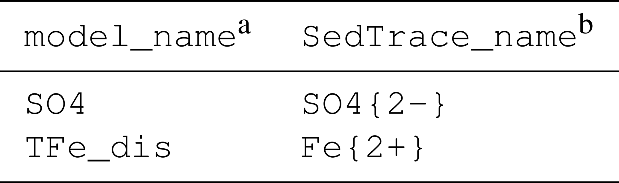
The values of m₀, m₁ and $D_i^{{\mathrm{md}}^{\mathrm{25}{}^{\circ }\mathrm{C}}}$ of selected dissolved substances compiled by Boudreau (1997) are stored in the database file /src/diffusion.xlsx. If a model substance is in the database, then the user simply needs to list it in the diffusion sheet, where their model_name given by the user needs to match the SedTrace_name in the database (Table 5). SedTrace will compute $D_i^{\mathrm{md}}$ automatically. If the model substance is not in the database, the user can either modify the database file to include it or directly supply $D_i^{\mathrm{md}}$ to parameters.

The example code for diffusion coefficient is as follows.
#--------------------------------------
# solute diffusivity
#--------------------------------------
DSO4 = 1.8034511184582917E+02 ./ (1.0 .- 2log.(phif)) # cm^2 yr^{-1} # Sediment diffusion coefficient

3.4 Total physical transport

SedTrace collects the discretized advective and diffusive fluxes as an interior transport matrix A (Am) by calling the fvcf() function, which performs the FV-CF discretization. The AC term in Eq. (5) is then computed. The code for the transport of SO₄ (AmSO4) is as follows.
#--------------------------------------
# Interior transport matrix
#--------------------------------------
AmSO4 = fvcf(phif, DSO4, uf, dx, Ngrid) # # Interior transport matrix of SO4
#--------------------------------------
# Transport term A*C
#--------------------------------------
mul!(dSO4, AmSO4, SO4) # dSO4 is the rate of change

3.5 Bio-irrigation

Bio-irrigation sources and sinks of a dissolved substance are modeled as a non-local exchange (Boudreau, 1997):

$$\begin{array}{}\text{(15)}& T_i^{\mathrm{bio}}=\mathit{\alpha }(C_i^{\mathrm{f}}-C_i^{\mathrm{BW}}),\end{array}$$

where α (alpha) is the bio-irrigation coefficient as a function of depth x and $C_i^{\mathrm{BW}}$ is the bottom-water concentration, both supplied to parameters. Previous studies have suggested that the bio-irrigation coefficient α is also substance-specific (Meile et al., 2005), but it is unknown how this effect should be parameterized. SedTrace thus does not consider it at the moment.

The code for the biological transport term of SO₄ is as follows.
#--------------------------------------
# bioirrigation parameters
#--------------------------------------
alpha = broadcast(x -> 10 * exp(-x / 2), x) # yr^{-1} # Bioirrigation coefficient
#--------------------------------------
# biological transport
#--------------------------------------
@.. dSO4 += alpha * (SO4BW - SO4)

3.6 Boundary conditions

At the SWI, for a solid substance ($C_i^{\mathrm{s}})$ users can specify a Robin boundary condition using the incoming flux ($F{C}_i^{{\mathrm{s}}^{\mathrm{0}}}$) (Boudreau, 1997),

$$\begin{array}{}\text{(16)}& {\left.-{\mathit{\varphi }}^{\mathrm{s}}{D}^{\mathrm{b}}{\displaystyle \frac{\partial C_i^{\mathrm{s}}}{\partial x}}\right|}_{x=\mathrm{0}}+{\left.{\mathit{\varphi }}^{\mathrm{s}}{v}^{\mathrm{s}}{C}_i^{\mathrm{s}}\right|}_{x=\mathrm{0}}=F{C}_i^{{\mathrm{s}}^{\mathrm{0}}},\end{array}$$

or a Dirichlet boundary condition using the concentration at the SWI ($C_i^{{\mathrm{s}}^{\mathrm{0}}}$):

$$\begin{array}{}\text{(17)}& {\left.C_i^{\mathrm{s}}\right|}_{x=\mathrm{0}}=C_i^{{\mathrm{s}}^{\mathrm{0}}}.\end{array}$$

At the SWI, for a dissolved substance ($C_i^{\mathrm{f}}$) users can specify a Robin boundary condition assuming the existence of a diffusive boundary layer (DBL) of thickness δ and the overlying bottom-water concentration of $C_i^{\mathrm{BW}}$ (Boudreau, 1997),

$$\begin{array}{}\text{(18)}& \begin{array}{rl}& {\left.-{\mathit{\varphi }}^{\mathrm{f}}{\displaystyle \frac{D_j^{i,\mathrm{md}}}{{\mathit{\theta }}^{\mathrm{2}}}}{\displaystyle \frac{\partial C_i^{\mathrm{f}}}{\partial x}}\right|}_{x=\mathrm{0}}+{\left.{\mathit{\varphi }}^{\mathrm{f}}{v}^{\mathrm{f}}{C}_i^{\mathrm{f}}\right|}_{x=\mathrm{0}}\\ & ={\displaystyle \frac{D_j^{i,\mathrm{md}}}{\mathit{\delta }}}(C_i^{\mathrm{BW}}-{\left.C_i^{\mathrm{f}}\right|}_{x=\mathrm{0}}),\end{array}\end{array}$$

or a Dirichlet boundary condition using the concentration at the SWI ($C_i^{{\mathrm{f}}^{\mathrm{0}}}$):

$$\begin{array}{}\text{(19)}& {\left.C_i^{\mathrm{f}}\right|}_{x=\mathrm{0}}=C_i^{{\mathrm{f}}^{\mathrm{0}}}.\end{array}$$

At the bottom of the model domain (x=L), users can specify either a Neumann or a Dirichlet boundary condition for model substances:

$$\begin{array}{}\text{(20)}& {\displaystyle }{\left.{\displaystyle \frac{\partial C_i^{\mathit{\xi }}}{\partial x}}\right|}_{x=L}=\mathrm{0},\text{(21)}& {\displaystyle }{\left.C_i^{\mathit{\xi }}\right|}_{x=L}=C_i^{{\mathit{\xi }}^L}.\end{array}$$

Here Eq. (20) assumes no concentration gradient at x=L.

The user specifies the type of boundary conditions in substances and provides the necessary parameters in parameters (Table 6). SedTrace will format the boundary conditions as

$$\begin{array}{}\text{(22)}& {\mathit{\alpha }}_{\mathrm{1}}{C}_i^{\mathit{\xi }}+a_{\mathrm{2}}{\displaystyle \frac{\partial C_i^{\mathit{\xi }}}{\partial x}}=a_{\mathrm{3}}.\end{array}$$

For example, setting the Robin boundary condition in Eq. (18) at the SWI for SO₄ (Table 1), SedTrace will compute $\mathit{\beta }=\frac{D_j^{i,\mathrm{md}}}{\mathit{\delta }}$ (beta), which is the mass transfer velocity, as well as ${\mathit{\alpha }}_{\mathrm{1}}^{\mathrm{0}}=\mathit{\beta }+{\mathit{\varphi }}^{\mathrm{f}}{v}^{\mathrm{f}}$, $a_{\mathrm{2}}^{\mathrm{0}}=-{\mathit{\varphi }}^{\mathrm{f}}\frac{D_j^{i,\mathrm{md}}}{{\mathit{\theta }}^{\mathrm{2}}}$ and $a_{\mathrm{3}}^{\mathrm{0}}=\mathit{\beta }{C}_i^{\mathrm{BW}}$ using δ (delta) and $C_i^{\mathrm{BW}}$ (SO4BW) from the parameters. The Neumann bottom boundary condition is simply ${\mathit{\alpha }}_{\mathrm{1}}^L=\mathrm{0}$, $a_{\mathrm{2}}^L=\mathrm{1}$ and $a_{\mathrm{3}}^L=\mathrm{0}$. SedTrace collects these coefficients into a Tuple (($a_{\mathrm{1}}^{\mathrm{0}},a_{\mathrm{2}}^{\mathrm{0}},a_{\mathrm{3}}^{\mathrm{0}})$, ($a_{\mathrm{1}}^L,a_{\mathrm{2}}^L,a_{\mathrm{3}}^L\left)\right)$, which is passed to fvcf_bc() to generate the homogeneous (BcAM, B) and nonhomogeneous (BcCm, b) parts of the boundary condition based on the FV-CF discretization. SedTrace then updates the right-hand side of Eq. (5) by adding the BC+b term. The code for SO₄ is as follows.
#--------------------------------------
# assemble boundary conditions
#--------------------------------------
BcSO4 = (
    (betaSO4 + phif[1]uf[1], -phif[1]DSO4[1], betaSO4 * SO4BW),
    (0.0, 1.0, 0.0),
) #  # Boundary condition of SO4
#--------------------------------------
# Boundary transport matrix
#--------------------------------------
BcAmSO4, BcCmSO4 = fvcf_bc(phif, DSO4, uf, dx, BcSO4, Ngrid) #  # Boundary transport matrix of SO4
#--------------------------------------
# Boundary terms
#--------------------------------------
dSO4[1] += BcAmSO4[1] * SO4[1] + BcCmSO4[1]
dSO4[Ngrid] += BcAmSO4[2] * SO4[Ngrid] + BcCmSO4[2]

4 Biogeochemical reactions

Biogeochemical reactions in diagenetic models can be classified as kinetic or equilibrium reactions (Boudreau, 1997; Meysman et al., 2003). The difference mainly lies in the reaction timescale: reactions that happen on much shorter timescales than physical transport are often treated as equilibrium rather than kinetic reactions. The user is free to add the kinetic reactions, while SedTrace has a specific user interface for two types of equilibrium reactions: acid dissociation for pH modeling and aqueous complexation–sorption for speciation modeling. SedTrace uses the direct substitution approach (DSA) to handle the equilibrium reactions, which performs better than other approaches when dealing with a highly coupled and stiff biogeochemical reaction network (Meysman et al., 2003).

4.1 Kinetic reactions

The summed rate of kinetic reactions for substance $C_i^{\mathit{\xi }}$ is

$$\begin{array}{}\text{(23)}& R_i=\sum _{\mathit{\eta }}{\mathit{\varphi }}^{\mathit{\eta }}/{\mathit{\varphi }}^{\mathit{\xi }}\sum _k{\mathit{\nu }}_i^{\mathit{\eta },k}{r}^{\mathit{\eta },k},\end{array}$$

where r^η,k is the rate of the kth reaction in units per volume of phase η, and ${\mathit{\nu }}_i^{\mathit{\eta },k}$ is the stoichiometry of the ith substance in this reaction. The unit of R_i is per volume of phase ξ. The convention of SedTrace is that homogeneous reactions between dissolved substances are in units per volume of fluid, while heterogeneous reactions between dissolved and solid substances and homogenous reactions between the solid substances are in units per volume of solid. Conversion between fluid and solid concentration units is done using the conversion factor ${\mathit{\varphi }}^{\mathrm{f}}/{\mathit{\varphi }}^{\mathrm{s}}$ (fluid to solid, pwtods) or ${\mathit{\varphi }}^{\mathrm{s}}/{\mathit{\varphi }}^{\mathrm{f}}$ (solid to fluid, dstopw). Kinetic reactions are added to the reactions sheet, including their chemical equations and rate expressions. SedTrace parses the reactions and re-assembles them into Julia code using Julia's Perl-compatible regular expression engine and the symbolic computing utility from the SymPy.jl package (Meurer et al., 2017).

4.1.1 Chemical equations

In SedTrace each model substance and its dissolved and adsorbed species need to have a code name and a chemical formula, supplied to the Excel sheets as noted in the tables. The code names are used in the code, and I suggest only using the Latin alphabet and “_” in the name. The formulae are necessary only when writing chemically balanced reaction equations. The code name and the chemical formula can be the same if (and only if) the chemical formula is an allowed Julia variable name, such as FeOOH but not Fe{2+}. The chemical formula of a substance should be written in the form of (E)[e](F)[f](G)[g]{h+}, where E/F/G are compounds, e/f/g are their stoichiometric coefficients and h is the number of charge. For example, the user can name organic matter POM and write its chemical formula as (CH2O)(NH3)[rNC](H3PO4)[rPC], where rNC and rPC are the $\mathrm{N}/\mathrm{C}$ and $\mathrm{P}/\mathrm{C}$ ratios. SedTrace allows parameterized stoichiometry, and the parameters rNC and rPC should be supplied to parameters. This feature makes it easy to perform model sensitivity tests since natural chemical compounds such as organic matter in marine sediments rarely have fixed stoichiometry.

SedTrace requires the user to write chemical equations in the form of a*A + b*B = c*C + d*D, where a/b/c/d are the stoichiometry coefficients of substances A/B/C/D, and the reactants are on the left-hand side. The user has two options when writing these equations, decided by the check column in the reactions sheet (Table 2), which informs SedTrace if the chemical balance of the equation should be checked. The user can write a chemically balanced equation using the chemical formulae of the model substances A/B/C/D and set check to 1. Or the user can leave check empty and write a heuristic equation without considering chemical balance using code names only or a mixture of code names and chemical formulae. SedTrace offers the second choice because it is common in the diagenetic literature to write heuristic reactions. This happens because of the complexity of biogeochemical reactions in marine sediment such that it is often not possible to know the exact chemical formula or reaction mechanism. An example heuristic chemical equations is POM = Carbon + rNC*NH3 + rPC*PO4 for organic matter remineralization.

SedTrace uses regular expressions to split the chemical equation into reactants and products, as well as identify the stoichiometry coefficients ${\mathit{\nu }}_i^{\mathit{\eta },k}$ and charges of the model substances. SedTrace further parses the equation down to the level of individual elements, identifying the stoichiometry of each element. The results are saved in model_parsing_diagnostics.xlsx that the user should check to make sure the parsing is correct. Here I show the parsing result of a more complex version of the Fe reduction reaction in Table 2. (CH2O)(NH3)[rNC](H3PO4)[rPC] + 4*FeOOH + (8+rNC-rPC)*H{+} = CO2 + rNC*NH4{+} + rPC*H2PO4{-} + 4*Fe{2+} + 7*H2O:
#--------------------------------------
# Parsing the chemical equation into reactants/products
#--------------------------------------

Row	species	stoichiometry	charge	role
	String	String	String	String
1	(CH2O)(NH3)	-1	0	reactant
	[rNC](H3PO4)
	[rPC]
2	FeOOH	-4	0	reactant
3	H	-(8+rNC-rPC)	+1	reactant
4	CO2	1	0	product
5	NH4	rNC	+1	product
6	H2PO4	rPC	-1	product
7	Fe	4	+2	product
8	H2O	7	0	product

#--------------------------------------
# Parsing the chemical equation into elements
# negative value indicates reactant
#--------------------------------------

Row	element	coef
	String	String
1	C	-1
2	H	-2
3	O	-1
4	N	(-rNC)
5	H	(-3*rNC)
6	H	(-3*rPC)
7	P	(-rPC)
8	O	(-4*rPC)
9	Fe	-4
10	O	-4
11	O	-4
12	H	-4
13	H	(-rNC + rPC - 8)
14	C	1
15	O	2
16	N	(rNC)
17	H	(4*rNC)
18	H	(2*rPC)
19	P	(rPC)
20	O	(4*rPC)
21	Fe	4
22	H	14
23	O	7

Since the stoichiometry may be parameterized, SedTrace uses symbolic computing to check the chemical balance if check = 1. Parameters like rNC and rPC are converted to Julia symbols of type SymPy.Sym. The sums of charge and mass are computed symbolically, and errors are thrown if the sums are not zero. If check is empty SedTrace will parse the equation and identify the stoichiometric coefficients, but it will not check the chemical balance.

4.1.2 Reaction rates

The string expressions of reaction rates, r^η,k in Eq. (23), supplied to the reactions sheet are copied and pasted as Julia code directly, and therefore they should be written only using the code names. For dissolution and precipitation reactions, the user can add the definition of saturation state in a separate column: Omega. SedTrace will allow dissolution or precipitation only when Omega < 1 or Omega > 1, respectively. However, an if Omega > 1, then the precipitate statement, i.e., a Heaviside step function, in the code induces numerical discontinuity, which can hurt numerical performance, especially when applying automatic differentiation to the code. SedTrace provides the option of approximating the Heaviside step function using the logistic function, which is continuously differentiable:

$$\begin{array}{}\text{(24)}& r_{\mathrm{pre}}^{\prime }=\left({\displaystyle \frac{\mathrm{1}}{\mathrm{2}}}\tanh \left(\mathit{\tau }(\mathrm{\Omega }-\mathrm{1})\right)+{\displaystyle \frac{\mathrm{1}}{\mathrm{2}}}\right)r_{\mathrm{pre}},\end{array}$$

where r_pre is a precipitation rate and the parameter τ controls how close the approximation is. By default τ=10³, which results in a sharp transition near saturation (Fig. 2). For example, the code for FeS precipitation rate RFeS_pre is as follows.
@.. Omega_RFeS_pre = Fe_eq * HS / (H * KspFeS)
# saturation state for precipitation
@.. RFeS_pre =
(tanh(1e3 * (Omega_RFeS_pre - 1.0)) / 2 + 0.5) *
(kFeSpre * (Omega_RFeS_pre - 1))
# precipitation rate

This option can be disabled during code generation (see Sect. 7).

To compute the summed reaction rate R_i in Eq. (23), SedTrace collects the stoichiometry coefficients ${\mathit{\nu }}_i^{\mathit{\eta },k}$ of the model substances in each kinetic reaction after parsing the chemical equations and applies the appropriate unit conversion factors (dstopw or pwtods). For example, code for the summed reaction rate S_FeOOH of Fe oxide is as follows.
@.. S_FeOOH = -4 * RFeOOHPOC + -2
* RFeOOHH2S

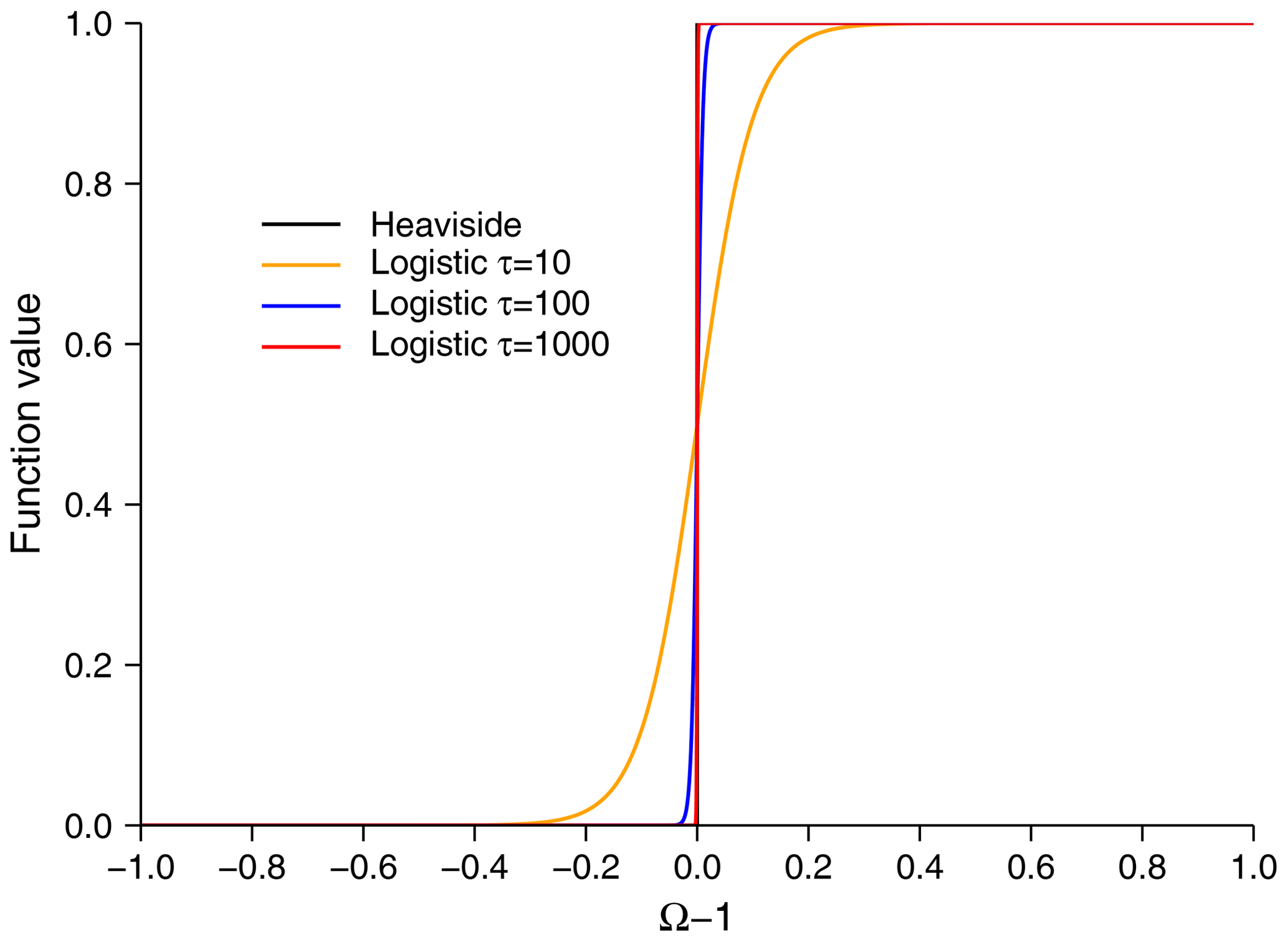
Figure 2 Approximating the Heaviside function using the logistic function. Here I show the results using different values of the parameter τ.

4.2 pH modeling

Traditionally diagenetic models enable pH modeling by combining the differential equations describing the time evolution of model substances together with the pH-dependent nonlinear algebraic equations of charge or alkalinity balance, forming a system of differential algebraic equations (Wang and Van Cappellen, 1996; Boudreau, 1996). However, this approach is not only numerically difficult, but it also does not give direct information on how model processes affect pH. SedTrace models pH using the DSA outlined by Hofmann et al. (2008, 2009, 2010). Under this approach, proton concentration is modeled dynamically, avoiding the challenge of solving DAEs while allowing detailed partitioning of pH changes to individual reaction and transport processes. The dynamic equation for proton concentration ([H⁺], free scale) is

$$\begin{array}{}\text{(25)}& {\displaystyle \frac{\partial }{\partial t}}\left[{\mathrm{H}}^{+}\right]=\left({\displaystyle \frac{\partial }{\partial t}}\text{TA}-\sum _l{\displaystyle \frac{\partial \text{TA}}{\partial {\text{EI}}_l}}{\displaystyle \frac{\partial }{\partial t}}{\text{EI}}_l\right)/{\displaystyle \frac{\partial \text{TA}}{\partial \left[{\mathrm{H}}^{+}\right]}},\end{array}$$

where TA is the total alkalinity (TA), and EI_l is the lth equilibrium invariant (EI). The EIs are composite variables, such as the total dissolved inorganic carbon (TCO₂). They are so named because they are invariant with respect to the equilibrium reaction rates.

The full definition of TA in seawater (Dickson et al., 2007) is

$$\begin{array}{}\text{(26)}& \begin{array}{rl}\text{TA}& =\left[{\mathrm{HCO}}_{\mathrm{3}}^{-}\right]+\mathrm{2}\left[{\mathrm{CO}}_{\mathrm{3}}^{\mathrm{2}-}\right]+\left[B{\left(\mathrm{OH}\right)}_{\mathrm{4}}^{-}\right]+\left[{\mathrm{OH}}^{-}\right]\\ & +\left[{\mathrm{HPO}}_{\mathrm{4}}^{\mathrm{2}-}\right]+\mathrm{2}\left[{\mathrm{PO}}_{\mathrm{4}}^{\mathrm{3}-}\right]+\left[{\mathrm{H}}_{\mathrm{3}}{\mathrm{SiO}}_{\mathrm{4}}^{-}\right]+\left[{\mathrm{NH}}_{\mathrm{3}}\right]\\ & +\left[{\mathrm{HS}}^{-}\right]-\left[{\mathrm{H}}^{+}\right]-\left[\mathrm{HF}\right]-\left[{\mathrm{HSO}}_{\mathrm{4}}^{-}\right]-\left[{\mathrm{H}}_{\mathrm{3}}{\mathrm{PO}}_{\mathrm{4}}\right].\end{array}\end{array}$$

To include all these species, SedTrace provides the following EIs:

$$\begin{array}{}\text{(27)}& {\displaystyle }{\mathrm{TCO}}_{\mathrm{2}}=\left[{\mathrm{HCO}}_{\mathrm{3}}^{-}\right]+\left[{\mathrm{CO}}_{\mathrm{3}}^{\mathrm{2}-}\right]+\left[{\mathrm{CO}}_{\mathrm{2}}\right],\text{(28)}& {\displaystyle }{\mathrm{TH}}_{\mathrm{2}}\mathrm{S}=\left[{\mathrm{H}}_{\mathrm{2}}\mathrm{S}\right]+\left[{\mathrm{HS}}^{-}\right],\text{(29)}& {\displaystyle }{\mathrm{TH}}_{\mathrm{3}}{\mathrm{BO}}_{\mathrm{3}}=\left[B{\left(\mathrm{OH}\right)}_{\mathrm{3}}\right]+\left[B{\left(\mathrm{OH}\right)}_{\mathrm{4}}^{-}\right],\text{(30)}& {\displaystyle }{\mathrm{TNH}}_{\mathrm{4}}=\left[{\mathrm{NH}}_{\mathrm{3}}\right]+\left[{\mathrm{NH}}_{\mathrm{4}}^{+}\right],\text{(31)}& {\displaystyle }\begin{array}{rl}{\mathrm{TH}}_{\mathrm{3}}{\mathrm{PO}}_{\mathrm{4}}& =\left[{\mathrm{H}}_{\mathrm{3}}{\mathrm{PO}}_{\mathrm{4}}\right]+\left[{\mathrm{H}}_{\mathrm{2}}{\mathrm{PO}}_{\mathrm{4}}^{-}\right]+\left[{\mathrm{HPO}}_{\mathrm{4}}^{\mathrm{2}-}\right]\\ & +\left[{\mathrm{PO}}_{\mathrm{4}}^{\mathrm{3}-}\right],\end{array}\text{(32)}& {\displaystyle }{\mathrm{THSO}}_{\mathrm{4}}=\left[{\mathrm{HSO}}_{\mathrm{4}}^{-}\right]+\left[{\mathrm{SO}}_{\mathrm{4}}^{\mathrm{2}-}\right],\text{(33)}& {\displaystyle }\mathrm{THF}=\left[\mathrm{HF}\right]+\left[{\mathrm{F}}^{-}\right],\text{(34)}& {\displaystyle }{\mathrm{TH}}_{\mathrm{4}}{\mathrm{SiO}}_{\mathrm{4}}=\left[{\mathrm{H}}_{\mathrm{4}}{\mathrm{SiO}}_{\mathrm{4}}\right]+\left[{\mathrm{H}}_{\mathrm{3}}{\mathrm{SiO}}_{\mathrm{4}}^{-}\right].\end{array}$$

Except for protons, the concentration in these equations refers to the total concentration, i.e., the sum of the concentrations of free and complexed species. It is usually unnecessary to include the entire set in diagenetic models. The user is free to choose any subset of this collection. The user adds the selected EIs to the substances sheet and specifies the type as dissolved_pH. Apart from supplying the boundary conditions, all other aspects of pH modeling are handled internally by SedTrace, requiring no user input. Based on the user's choice, SedTrace defines TA as a subset of the full definition in Eq. (26). For example, in SimpleFe TCO₂ and TH₂S are selected (Table 1), and then $\text{TA}=\left[{\mathrm{HCO}}_{\mathrm{3}}^{-}\right]+\mathrm{2}\left[{\mathrm{CO}}_{\mathrm{3}}^{\mathrm{2}-}\right]+\left[{\mathrm{HS}}^{-}\right]+\left[{\mathrm{OH}}^{-}\right]-\left[{\mathrm{H}}^{+}\right]$. H⁺ and OH⁻ are always included by default.

SedTrace uses EquilibriumInvariant to store the information of the EIs, including the analytical expressions to compute the concentrations of the individual species listed in Eqs. (27) to (34), their coefficients in Eq. (26), and the expressions to compute $\frac{\partial \text{TA}}{\partial {\text{EI}}_l}$ and $\frac{\partial \text{TA}}{\partial \left[{\mathrm{H}}^{+}\right]}$, for example TCO₂.
struct EquilibriumInvariant
name::String # name of EI
species::Vector{String} # species
charge::Vector{String} # charges of the species
expr::Vector{String} # expression to compute the species concentration
coef::Vector{String} # coefficient of species in TA definition
dTAdEI::String # expression to compute dTA/dEI
dTAdH::String # expression to compute this EI's
contribution to dTA/dH
diss_const::VectorString # acid dissociation
constants
end
# TCO2 for example
EquilibriumInvariant(
"TCO2",
["HCO3", "CO3", "CO2"],
["{-}","{2-}",""],
[ "H * KCO2 * TCO2 / (H^2 + H * KCO2
+ KCO2 * KHCO3)",
"KCO2 * KHCO3 * TCO2 / (H^2 + H * KCO2 + KCO2 * KHCO3)",
"H^2 * TCO2 / (H^2 + H * KCO2 + KCO2 * KHCO3)",
],
["1", "2", "0"],
"KCO2*(H + 2*KHCO3)/(H^2 + H*KCO2 + KCO2
* KHCO3)",
"-KCO2*TCO2*(H^2 + 4*H*KHCO3 + KCO2*KHCO3)/
(H^2 + H*KCO2 + KCO2*KHCO3)^2",
["KCO2","KHCO3"]
)

SedTrace stores precomputed dissociation constants (on the free proton scale) on high-resolution grids of salinity, temperature and pressure in /src/dissociation_constant.jld2 following the Guide to best practices for ocean CO₂ measurements (Dickson et al., 2007) as implemented in the seacarb package (Gattuso et al., 2021). During code generation, SedTrace will compute the dissociation constants at the in situ salinity, temperature and pressure by interpolation. In the case of SimpleFe, the dissociation constant of H₂O (KH2O), the first (KCO2) and second (KHCO3) dissociation constants of H₂CO₃, and the first dissociate constant of H₂S (KH2S) are computed as follows.
#————————————–
# Acid dissociation constants
#————————————–
KH2O = 7.9445878598109790E-15 #H 1th dissociation constant
KCO2 = 8.3698755808176183E-07 #TCO2 1th dissociation constant
KHCO3 = 4.6352156109843975E-10 #TCO2 2th dissociation constant
KH2S = 1.2845618784784923E-07 #H2S 1th dissociation constant

Given the concentrations of EIs and protons, SedTrace computes the concentrations of the individual species, as well as their transport and boundary condition terms following Sect. 3. SedTrace uses species-specific diffusion coefficients computed following Sect. 3.3. Many diagenetic models transport EIs and TA using the diffusion coefficients of the dominant species (for example, using the diffusion coefficient of HCO${}_{\mathrm{3}}^{-}$ to represent all TCO₂ species) or a fixed weighted average of the diffusion coefficients of the individual species (for example, computing a bulk diffusion coefficient for TCO₂ using the weighted average of the diffusion coefficients of HCO${}_{\mathrm{3}}^{-}$, CO${}_{\mathrm{3}}^{\mathrm{2}-}$ and CO₂ where the weight is fixed based on bottom-water speciation). However, studies have shown that these practices may lead to modeled pore water pH being different than using the species-specific diffusion coefficient (Luff et al., 2001; Jourabchi et al., 2005). In the SimpleFe example, code for the transport and boundary conditions of HCO${}_{\mathrm{3}}^{-}$ is as follows.
@.. HCO3 = H * KCO2 * TCO2 / (H^2 + H
* KCO2 + KCO2 * KHCO3)
mul!(HCO3_tran, AmHCO3, HCO3)
HCO3_tran[1] += BcAmHCO3[1] * HCO3[1]
+ BcCmHCO3[1]
HCO3_tran[Ngrid] += BcAmHCO3[2]
* HCO3[Ngrid] + BcCmHCO3[2]
@.. HCO3_tran += alpha * (HCO30 - HCO3)

SedTrace then computes the transport and kinetic reaction terms of TA and EIs by summing over the species:

$$\begin{array}{}\text{(35)}& {\displaystyle \frac{\partial }{\partial t}}{\mathit{\varphi }}^{\mathrm{f}}{\text{EI}}_l+\sum _m{T}_{{\mathrm{EI}}_l^m}=\sum _{\mathit{\eta }}{\mathit{\varphi }}^{\mathit{\eta }}\sum _k\left(\sum _m{\mathit{\nu }}_{{\mathrm{EI}}_l^m}^{\mathit{\eta },k}\right)r^{\mathit{\eta },k},\text{(36)}& {\displaystyle \frac{\partial }{\partial t}}{\mathit{\varphi }}^{\mathrm{f}}\text{TA}+\sum _n{\mathit{\zeta }}_n{T}_{{\mathrm{TA}}^n}=\sum _{\mathit{\eta }}{\mathit{\varphi }}^{\mathit{\eta }}\sum _k\left(\sum _n{\mathit{\zeta }}_n{\mathit{\nu }}_{{\mathrm{TA}}^n}^{\mathit{\eta },k}\right)r^{\mathit{\eta },k},\end{array}$$

where ${\text{EI}}_l^m$ is the mth species of EI_l, TAⁿ is the nth species in the definition of TA and ζ_n is its coefficient in Eq. (26). ${\mathit{\nu }}_{{\mathrm{EI}}_l^m}^{\mathit{\eta },k}$ and ${\mathit{\nu }}_{{\mathrm{TA}}^n}^{\mathit{\eta },k}$ are the stoichiometric coefficients of these species in the kinetic reaction r^η,k, respectively.

The user can use the individual species when writing the chemical equations of the kinetic reaction rates. SedTrace will parse the equations and identify ${\mathit{\nu }}_{{\mathrm{EI}}_l^m}^{\mathit{\eta },k}$ and ${\mathit{\nu }}_{{\mathrm{TA}}^n}^{\mathit{\eta },k}$ automatically. For example, SedTrace recognizes that for the reaction RFeS_pre in Table 2, the stoichiometric coefficient of TH₂S is ${\mathit{\nu }}_{{\mathrm{HS}}^{-}}=-\mathrm{1}$, and the stoichiometric coefficient of TA is ${\mathit{\nu }}_{{\mathrm{HS}}^{-}}-{\mathit{\nu }}_{{\mathrm{H}}^{+}}=-\mathrm{2}$. For the SimpleFe model the reaction-transport code for TA and EIs is as follows.
# Transport of EIs
@.. dTCO2 = HCO3_tran + CO3_tran + CO2_tran
@.. dTH2S = H2S_tran + HS_tran
# Transport of TA
@.. TA_tran = -1 * H_tran + 1 * OH_tran
@.. TA_tran += 1 * HCO3_tran + 2 * CO3_tran + 0 * CO2_tran
@.. TA_tran += 0 * H2S_tran + 1 * HS_tran
# Kinetic reaction rates of EIs
@.. S_TCO2 = 1 * RFeOOHPOC * dstopw + 1 * RSO4POC * dstopw
@.. S_TH2S =
    1 / 2 * RSO4POC * dstopw + -1 * RFeOOHH2S * dstopw + -1 * RFeS_pre
# Kinetic reaction rates of TA
@.. S_TA =
    8 * RFeOOHPOC * dstopw + 1 * RSO4POC * dstopw + 4 * RFeOOHH2S * dstopw + -1 * RFeS_pre
@.. S_TA += -1 * RFeS_pre

SedTrace does not explicitly model TA; rather, Eqs. (35) and (36) are substituted back into Eq. (25) to eliminate the TA terms to arrive at a diagenetic equation of [H⁺]:

$$\begin{array}{}\text{(37)}& {\displaystyle }{T}_{\mathrm{H}}=(\sum _n{\mathit{\zeta }}_n{T}_{{\mathrm{TA}}^n}-\sum _l{\displaystyle \frac{\partial \text{TA}}{\partial {\text{EI}}_l}}\sum _m{T}_{{\mathrm{EI}}_l^m})/{\displaystyle \frac{\partial \text{TA}}{\partial \left[{\mathrm{H}}^{+}\right]}},\text{(38)}& {\displaystyle }\begin{array}{rl}{R}_{\mathrm{H}}& =\sum _{\mathit{\eta }}{\mathit{\varphi }}^{\mathit{\eta }}/{\mathit{\varphi }}^{\mathrm{f}}\sum _k\left(\sum _n{\mathit{\zeta }}_n{\mathit{\nu }}_{{\mathrm{TA}}^n}^{\mathit{\eta },k}\right.\\ & \left.-\sum _l{\displaystyle \frac{\partial \text{TA}}{\partial {\text{EI}}_l}}\sum _m{\mathit{\nu }}_{{\mathrm{EI}}_l^m}^{\mathit{\eta },k}\right)/{\displaystyle \frac{\partial \text{TA}}{\partial \left[{\mathrm{H}}^{+}\right]}}{r}^{\mathit{\eta },k},\end{array}\text{(39)}& {\displaystyle \frac{\partial }{\partial t}}{\mathit{\varphi }}^{\mathrm{f}}\left[{\mathrm{H}}^{+}\right]+T_{\mathrm{H}}={\mathit{\varphi }}^{\mathrm{f}}{R}_{\mathrm{H}}.\end{array}$$

In the terminology of Hofmann et al. (2010), $-\frac{\partial \text{TA}}{\partial \left[{\mathrm{H}}^{+}\right]}$ is the buffer factor and ${\mathit{\nu }}_{\mathrm{H}}^{\mathit{\eta },k}=-(\sum _n{\mathit{\zeta }}_n{\mathit{\nu }}_{{\mathrm{TA}}^n}^{\mathit{\eta },k}-\sum _l\frac{\partial \text{TA}}{\partial {\text{EI}}_l}\sum _m{\mathit{\nu }}_{{\mathrm{EI}}_l^m}^{\mathit{\eta },k})$ is the fractional stoichiometric coefficient of protons in the kinetic reaction r^η,k. Equations (37) to (39) show that the advantage of DSA is that the rate of pH change can be clearly partitioned at the level of individual species and reactions.

The user only needs to supply the boundary conditions for the EIs and pH. SedTrace will internally compute the boundary conditions for the individual species and form the transport terms in Eq. (37) according to Sect. 3. The user can use the EIs or the individual species when writing the chemical reactions. SedTrace will set the stoichiometry coefficients in Eq. (38) automatically according to Sect. 4.1. For the SimpleFe model the code for Eqs. (37) to (39) is as follows.
#  dTA/dEIs
@.. dTA_dTCO2 = KCO2 * (H + 2 * KHCO3)
/ (H^2 + H * KCO2 + KCO2 * KHCO3)
@.. dTA_dTH2S = KH2S / (H + KH2S)
#  dTA/dH
@.. dTA_dH = -(H^2 + KH2O) / H^2
@.. dTA_dH +=
-KCO2 * TCO2 * (H^2 + 4 * H * KHCO3
+ KCO2 * KHCO3) /
(H^2 + H * KCO2 + KCO2 * KHCO3)^2
@.. dTA_dH += -KH2S * TH2S / (H + KH2S)^2
# transport of individual species
mul!(HCO3_tran, AmHCO3, HCO3)
HCO3_tran[1] += BcAmHCO3[1] * HCO3[1]
+ BcCmHCO3[1]
HCO3_tran[Ngrid] += BcAmHCO3[2]
* HCO3[Ngrid] + BcCmHCO3[2]
@.. HCO3_tran += alpha * (HCO30 - HCO3)
# ... other species
# transport of EIs
@.. dTCO2 = HCO3_tran + CO3_tran
+ CO2_tran
@.. dTH2S = H2S_tran + HS_tran
# transport of TA
@.. TA_tran = -1 * H_tran + 1 * OH_tran
@.. TA_tran += 1 * HCO3_tran + 2
* CO3_tran + 0 * CO2_tran
@.. TA_tran += 0 * H2S_tran + 1 * HS_tran
#  transport of proton
@.. dH = TA_tran
@.. dH -= dTCO2 * dTA_dTCO2
@.. dH -= dTH2S * dTA_dTH2S
@.. dH = dH / dTA_dH
# kinetic reaction rates of proton
@.. S_H = S_TA
@.. S_H -= S_TCO_2 * dTA_dTCO_2
@.. S_H -= S_TH2S * dTA_dTH2S
@.. S_H = S_H / dTA_dH


The apparent dissociation constants depend not only on ionic strength but also composition (Zeebe and Wolf-Gladrow, 2001). The assumption of the pH modeling laid out above is that the ionic medium of interest has a similar major ion composition as modern seawater; otherwise, the dissociation constants will not be applicable. Thus, SedTrace 1.0 is not suitable for modeling pore water with a major ion composition considerably different from modern seawater, which may happen in late diagenesis or in extreme or ancient environments.

4.3 Speciation modeling

Speciation of TEIs in diagenetic models is highly diverse and there is a lack of universally accepted practice. As such, SedTrace leaves the model decision to the user, while only requiring the user to format the input consistently. Thus, the responsibility of choosing a suitable set of aqueous and adsorbed species, equilibrium constants, and speciation equations lies with the user, whereas SedTrace is used to convert user input to code.

In the DSA of speciation modeling, SedTrace models the total concentration of a model substance (M^T in unit of per volume fluid), which is the sum of the total dissolved (M^f in units per volume of fluid) and total adsorbed (M^s in units per volume of solid) concentrations:

$$\begin{array}{}\text{(40)}& M^{\mathrm{T}}=M^{\mathrm{f}}+{\displaystyle \frac{{\mathit{\varphi }}^{\mathrm{s}}}{{\mathit{\varphi }}^{\mathrm{f}}}}{M}^{\mathrm{s}},\end{array}$$

and M^fand M^s are themselves sums of the concentrations of individual dissolved and adsorbed species, respectively.

To indicate that speciation modeling is required for a model substance, the user needs to specify dissolved_speciation in the type column in the substances sheet (Table 1) and provide the dissolved and adsorbed speciation information in the speciation (Table 3) and adsorption (Table 4) sheets. The name given in the substances sheet is the code name of the total concentration M^T. Internally SedTrace will set the code names of the total dissolved M^f and total adsorbed M^s concentrations by appending the postfix _dis and _ads to the code name of the model substance. For example, the user names the total Fe TFe in SimpleFe, and SedTrace will name the total dissolved and adsorbed Fe TFe_dis and TFe_ads, respectively. The code names (column dissolved) and chemical formulae (column formula) of the individual dissolved species should be supplied to speciation (Table 3). The code names (column adsorbed) of the individual adsorbed species should be supplied to adsorption (Table 4), but no chemical formula for the adsorbed species is needed.

The user can add the dissolved speciation reaction of a trace element M of the following format to the column equation in speciation (Pierrot and Millero, 2017):

$$\begin{array}{}\text{(41)}& M+q\times L_p⟺M(L_p{)}_q,\end{array}$$

which describes complexation with the pth dissolved ligand L_p to form aqueous species M(L_p)_q, and q is the number of the ligand in the complex. Assuming local equilibrium, the concentration of the complexed species is

$$\begin{array}{}\text{(42)}& \left[M\right(L_p{)}_q]=K_{M(L_p{)}_q}[M]{\left[L_p\right]}^q,\end{array}$$

where $K_{M(L_p{)}_q}$ is the apparent equilibrium constant supplied to column logK, and [M] is the concentration of the base species (e.g., free ion) M. [M^f] is the sum of the concentrations of the base and complexed species:

$$\begin{array}{}\text{(43)}& \left[M^{\mathrm{f}}\right]=\left[M\right](\mathrm{1}+\sum _p\sum _q{K}_{M(L_p{)}_q}{\left[L_p\right]}^q).\end{array}$$

In the speciation sheet, the base species is indicated by writing a trivial speciation equation such as Fe{2+} = Fe{2+} with logK = 0 in the SimpleFe model where free Fe²⁺ is the chosen base species of TFe (Table 3). SedTrace will parse and check the chemical balance of the equations as discussed in Sect. 4.1.1. The dissolved ligands have to be modeled or specified by users. In SimpleFe [HS⁻] is computed as part of the pH model, and the concentration of Cl⁻ is not modeled but deemed a constant and supplied to parameters. SedTrace 1.0 does not model the speciation of the ligands, and thus [L_p] in Eq. (42) refers to the total dissolved ligand concentrations. Therefore the apparent equilibrium constant supplied by the user needs to be precomputed using the total activity coefficients of model species based on ion pairing or Pitzer models (Pierrot and Millero, 2017; Millero and Schreiber, 1982; Zeebe and Wolf-Gladrow, 2001). This is a limitation of SedTrace 1.0 which I plan to resolve in the future.

The formulation of adsorption in the literature of diagenetic modeling is also diverse (Boudreau, 1997; Berner, 1980; Wang and Van Cappellen, 1996; Katsev et al., 2006). The challenge lies in the fact that the surface properties of sedimentary particles are poorly known. SedTrace thus does not constrain the formulation of adsorption and lets the user specify the concentrations of the adsorbed species directly.

In the adsorption sheet (Table 4), each row should list the adsorption of one dissolved species onto one surface. The user names the adsorbed species in the adsorbed column, the dissolved species to be adsorbed in the dissolved column and the surface to be adsorbed onto in the surface column. All three columns should contain code names only. The user then supplies a mathematical expression f^ads to compute the adsorbed species concentration in the expression column as a function of the concentrations of the dissolved species and surface:

$$\begin{array}{}\text{(44)}& \left[M^{\mathrm{s}}\equiv S_{\mathit{\kappa }}^{\mathit{\lambda }}\right]=f^{\mathrm{ads}}\left(\right[M^{\mathrm{dis}}],[\equiv S_{\mathit{\kappa }}\left]\right),\end{array}$$

where $[M^{\mathrm{s}}\equiv S_{\mathit{\kappa }}^{\mathit{\lambda }}]$ is the concentration of the λth dissolved species adsorbed onto the κth particle surface ≡S_κ. The dissolved species M^dis can be one of M, M(L_p)_q or M^f.

The term “surface” is used heuristically here and can refer to any modeled solid substance. For example, in the SimpleFe model (Table 4), Fe is adsorbed onto POC, and the expression for the adsorbed species is Fe_ads = KFe_ads*POC*TFe_dis, where the adsorption is assumed to be indifferent to the dissolved speciation, and thus the total dissolved Fe concentration TFe_dis (M^f) is used. The adsorption constant KFe_ads here is an apparent constant specific to the user's model decision and needs to be provided to the parameters sheet. The concentration of adsorbed species could sometimes be independent of any surface: for example, in the classic linear isothermal used by many diagenetic models (Berner, 1980) such that Fe_ads = KFe_ads*TFe_dis. In this case the surface column should be left empty.

SedTrace will group the adsorbed species by surface and compute the total concentration adsorbed onto the surface ≡S_κ ($\left[M_{\mathit{\kappa }}^{\mathrm{s}}\right]$, “empty surface” is a special surface) and the total concentration adsorbed onto all surfaces ([M^s]):

$$\begin{array}{}\text{(45)}& {\displaystyle }\left[M_{\mathit{\kappa }}^{\mathrm{s}}\right]={\sum }_{\mathit{\lambda }}[M^{\mathrm{s}}\equiv S_{\mathit{\kappa }}^{\mathit{\lambda }}],\text{(46)}& {\displaystyle }\left[M^{\mathrm{s}}\right]={\sum }_{\mathit{\kappa }}\left[M_{\mathit{\kappa }}^{\mathrm{s}}\right].\end{array}$$

Internally SedTrace creates a code name for $M_{\mathit{\kappa }}^{\mathrm{s}}$ by appending the postfix ads_surface to the substance name: for example, TFe_ads_POC for the total Fe adsorbed onto POC. If the surface is empty, the code name for this adsorbed species is created by appending the postfix _ads_nsf to the substance name: for example, TFe_ads_nsf for the linear isothermal case.

To generate the speciation code, SedTrace solves Eqs. (40) to (46) using the solveset function of solving systems of symbolic nonlinear equations from SymPy.jl (Meurer et al., 2017). To do so the user-supplied expression f^ads needs to be analytically invertible. The result is a set of symbolic expressions to compute [M], [M(L_p)_q], [M^f], $[M^{\mathrm{s}}\equiv S_{\mathit{\kappa }}^{\mathit{\lambda }}$], $\left[M_{\mathit{\kappa }}^{\mathrm{s}}\right]$ and [M^s] using [M^T], [L_p], [≡S_κ] and the equilibrium constants, which are converted to Julia code.

The symbolic derivation starts by rewriting Eq. (44) to substitute [M] and [M(L_p)_q] by [M^f] using Eqs. (42) and (43). Together with Eqs. (40), (45) and (46), SedTrace derives an expression to compute [M^f] using [M^T] and [≡S_κ]. In the case of TFe_dis in the SimpleFe model the code is as follows.
#  Concentrations of total dissolved species
@.. TFe_dis = TFe / (KFe_ads * POC * dstopw + 1)

Substituting this expression back to Eqs. (42) and (43), SedTrace derives the expressions to compute [M] and [M(L_p)_n] using [M^f] and [L_p]. The code for the individual dissolved Fe species is as follows.
#  Concentrations of the individual dissolved species
@.. Fe_aq =
3.98107170553497e-6 * TFe_dis / (
0.01778279410038921 * CO3
+ 3.019951720402014e-6 * Cl + 1.0
* HS +
3.630780547701011e-5 * SO4
+ 3.98107170553497e-6
)
@.. FeCl_aq =
3.019951720402014e-6 * Cl * TFe_dis / (
0.01778279410038921 * CO3
+ 3.019951720402014e-6 * Cl + 1.0
* HS +
3.630780547701011e-5 * SO4
+ 3.98107170553497e-6
)
@.. FeSO4_aq =
3.630780547701011e-5 * SO4 * TFe_dis / (
0.01778279410038921 * CO3
+ 3.019951720402014e-6 * Cl + 1.0
* HS
+
3.630780547701011e-5 * SO4
+ 3.98107170553497e-6
)
@.. FeCO3_aq =
0.01778279410038921 * CO3 * TFe_dis / (
0.01778279410038921 * CO3
+ 3.019951720402014e-6 * Cl + 1.0
* HS
+
3.630780547701011e-5 * SO4
+ 3.98107170553497e-6
)
@.. FeHS_aq =
1.0 * HS * TFe_dis / (
0.01778279410038921 * CO3
+ 3.019951720402014e-6 * Cl + 1.0
* HS
+
3.630780547701011e-5 * SO4
+ 3.98107170553497e-6
)
The user may not need to compute the concentrations of all species; for example, in this example only the concentration of the free species Fe_aq is needed. To choose the species whose concentrations are required by the model, set the value to 1 in the code column in the speciation sheet.

SedTrace then computes $\left[M^{\mathrm{s}}\equiv S_{\mathit{\kappa }}^{\mathit{\lambda }}\right]$, $\left[M_{\mathit{\kappa }}^{\mathrm{s}}\right]$ and [M^s] using [M], [M^f], [M(L_p)_n] and [≡S_κ] based on Eqs. (44) to (46); for example, the code for the individual and total adsorbed Fe species is as follows.
#  Concentrations of the individual adsorbed species
@.. Fe_ads = KFe_ads * POC * TFe_dis
#  Concentrations of the total adsorbed species onto each surface
@.. TFe_ads_POC = Fe_ads
#  Concentrations of the total adsorbed species
@.. TFe_ads = Fe_ads

In the next step, SedTrace computes the transport and reaction terms for M^T using M^f and M^s:

$$\begin{array}{}\text{(47)}& {\displaystyle \frac{\partial }{\partial t}}{\mathit{\varphi }}^{\mathrm{f}}\left[M^{\mathrm{T}}\right]+T_{M^{\mathrm{f}}}+T_{M^{\mathrm{s}}}=\sum _{\mathit{\eta }}{\mathit{\varphi }}^{\mathit{\eta }}\sum _k{\mathit{\nu }}_{M^{\mathrm{T}}}^{\mathit{\eta },k}{r}^{\mathit{\eta },k}.\end{array}$$

$T_{M^{\mathrm{f}}}$ is the transport of total dissolved species summed over individual species. SedTrace uses the same diffusion coefficients for the dissolved species, as the diffusivities of the aqueous complexes are generally not known. $T_{M^{\mathrm{s}}}$ is the transport of the total adsorbed species summed over individual species, which are subject to the same transport mechanism like normal solid substances. The user needs to supply two sets of boundary conditions when modeling M^T. The boundary conditions of M^f are supplied to the substances sheet, and the boundary conditions of M^s are supplied to the adsorption sheet.

When writing the chemical equations and rate expressions of the kinetic reactions, the user can use the code name or chemical formula of any of the following: M, M(L_p)_q, M^f, $M^{\mathrm{s}}\equiv S_{\mathit{\kappa }}^{\mathit{\lambda }}$, $M_{\mathit{\kappa }}^{\mathrm{s}}$, M^s or M^T. SedTrace will parse the reactions and set the stoichiometric coefficient for M^T (${\mathit{\nu }}_{M^{\mathrm{T}}}^{\mathit{\eta },k})$. The reactive-transport code for TFe in the SimpleFe model is as follows.
# Transport and boundary condition of total dissolved concentration
mul!(TFe_dis_tran, AmTFe_dis, TFe_dis)
TFe_dis_tran[1] += BcAmTFe_dis[1] * TFe_dis[1] + BcCmTFe_dis[1]
TFe_dis_tran[Ngrid] += BcAmTFe_dis[2] * TFe_dis[Ngrid] + BcCmTFe_dis[2]
# Transport and boundary condition of total adsorbed concentration
mul!(TFe_ads_tran, AmTFe_ads, TFe_ads)
TFe_ads_tran[1] += BcAmTFe_ads[1] * TFe_ads[1] + BcCmTFe_ads[1]
TFe_ads_tran[Ngrid] += BcAmTFe_ads[2] * TFe_ads[Ngrid] + BcCmTFe_ads[2]
# Transport of total concentration
@.. dTFe = TFe_dis_tran * 1 + TFe_ads_tran * dstopw
@.. dTFe += alpha * (TFe_dis0 - TFe_dis)
# Reaction rate of total concentration
@.. S_TFe = 4 * RFeOOHPOC * dstopw + 2 * RFeOOHH2S * dstopw + -1 * RFeS_pre

4.4 Sediment age

The user may sometimes need to know the sediment age. Use cases may rise, for example, when using the continuum reactivity model for organic carbon remineralization (Boudreau et al., 2008):

$$\begin{array}{}\text{(48)}& k_{\mathrm{POC}}={\displaystyle \frac{\mathit{\zeta }}{a_{\mathrm{0}}+a_t}},\end{array}$$

where k_POC is the reaction rate constant of organic carbon, ζ is the parameter controlling the shape of the gamma distribution of reactivity, a₀ is the initial age of organic carbon, and a_t is the duration of remineralization. Users may use sediment age in placement of a_t (Freitas et al., 2021).

The diagenetic equation for sediment age is (Meile and Van Cappellen, 2005)

$$\begin{array}{}\text{(49)}& {\displaystyle \frac{\partial }{\partial t}}{\mathit{\varphi }}^{\mathrm{s}}\text{Age}+{\displaystyle \frac{\partial }{\partial x}}{\mathit{\varphi }}^{\mathrm{s}}{v}^{\mathrm{s}}\text{Age}-{\displaystyle \frac{\partial }{\partial x}}{\mathit{\varphi }}^{\mathrm{s}}{D}^{\mathrm{b}}{\displaystyle \frac{\partial \text{Age}}{\partial x}}={\mathit{\varphi }}^{\mathrm{s}}.\end{array}$$

The top boundary condition of sediment age can be specified as Robin or Dirichlet type. If specifying a zero incoming flux, the modeled age can be interpreted with respect to the incoming sediments, the age of which is zero. If specifying a zero age at the SWI, the modeled age is set to zero whenever sediments make contact with the SWI. The bottom boundary condition of sediment age is specified as ${\left.\frac{\partial \text{Age}}{\partial x}\right|}_{x=L}=\frac{\mathrm{1}}{{\left.v^{\mathrm{s}}\right|}_{x=L}}$ to be consistent with the burial velocity. The use can add Age to the substances sheet with proper boundary conditions to enable sediment age modeling.

5 Julia code files

The code generated by SedTrace is assembled into five Julia files (Fig. 1): parm.jl and parm.struct.jl containing the model parameters, cache.jl containing the model cache, reactran.jl containing the reactive-transport code, and jactype.jl containing the sparsity pattern of the Jacobian matrix.

5.1 Parameters

The user-supplied parameters in the parameters sheet, and those computed internally by SedTrace, are included in parm.jl. Parameters that are directly needed by the ODE function in Eq. (5) are further packed into a container, called ParamStruct, within the module Param inside parm.struct.jl using the Julia package Parameters.jl (Werder, 2022a). For instance, the diffusion coefficients are not needed by Eq. (5) directly and are thus only included in parm.jl. The transport matrix A, which incorporates the diffusion coefficients, is needed directly by Eq. (5) and is thus included in ParamStruct. This container makes it easier to pass and modify parameters during model simulations. For the SimpleFe model the code of the ParamStruct is as follows.
@with_kw mutable struct ParamStruct{ T} # T is a Parametric Type
# only showing a few entries
TFeID::StepRange{ Int64,Int64} = TFeID # index of TFe
  AmTFe_dis::Tridiagonal{ T,Vector{ T} } = AmTFe_dis # transport matrix of TFe
    TFe_dis0::T = TFe_dis0 # top boundary condition of TFe
    kFeSpre::T = kFeSpre # FeS precipitation rate constant
end

5.2 Cache

The code generation process creates many intermediate variables, which could cause repeated memory allocation during model simulation. Technically, they can be eliminated by substitution using Symbolic computing, but it would render the code unreadable. SedTrace preserves them for code clarity and pre-allocates memories for them when initiating the model so the memories can be reused.

During code generation, SedTrace keeps track of which variables are intermediate variables. SedTrace adds them to a container Reactran within the module Cache inside cache.jl and pre-allocates their memories using the package PreallocationTools.jl (Rackauckas and Nie, 2017). The cache is compatible with the dual number type used by the package ForwardDiff.jl, so automatic differentiation can be applied to the code (Revels et al., 2016).
mutable struct Reactran{ T} # T is a Parametric Type
  TFe_dis::PreallocationTools.DiffCache{ Array{ T,1} ,Array} T,1} }
  FeCl_aq::PreallocationTools.DiffCache{ Array{ T,1} ,Array{ T,1} }
...... # other intermediate variables
end

5.3 ODE function

The reactran.jl file contains a function function(f::Cache.Reactran)(dC, C, parms:: Param.ParamStruct, t), which includes the reactive-transport code to update $\frac{\mathrm{d}}{\mathrm{d}t}\mathit{C}$ (dC) in Eq. (5) at time t in place, given the current model state vector C and parameters parms. This function is compatible with the ODE solvers from DifferentialEquations.jl (Rackauckas and Nie, 2017) and the automatic differentiation tools in ForwardDiff.jl (Revels et al., 2016).

This function is assembled in the following sequence: (1) unpack the parameters contained in parms using the package UnPack.jl (Werder, 2022b); (2) retrieve pre-allocated cache; (3) compute the transport and boundary condition terms of model substances that do not require speciation; (4) compute pH, EI speciation, and related transport and boundary condition terms; (5) compute the speciation of model substances that require speciation, as well as their transport and boundary condition terms; (6) compute the individual kinetic reaction rates and the summed rates for model substances. A code skeleton for SimpleFe model is shown here.
function (f::Cache.Reactran)(dC, C, parms::Param.ParamStruct, t)
#--------------------------------------
    #  Parameters
    #--------------------------------------
@unpack TFeID,
#...... other parameters
    kFeSpre = parms
    #--------------------------------------
    #  Cache
    #--------------------------------------
TFe_dis = PreallocationTools.get_tmp (f.TFe_dis, C)
#...... other caches
    #--------------------------------------
    #  Model state
    #--------------------------------------
    TFe = @view C[TFeID]
dTFe = @view dC[TFeID]
#...... other model substances
    #--------------------------------------
    #  Transport of solid and dissolved substances see Sect. 3.4
#--------------------------------------
#--------------------------------------
    #  pH code see Sect. 4.2
    #--------------------------------------
    #--------------------------------------
    #  Speciation code see Sect. 4.3
    #--------------------------------------
#  Concentrations of adsorbed/dissolved species
#  Transport of adsorbed/dissolved species
@.. dTFe = TFe_dis_tran * 1 + TFe_ads_tran * dstopw
    #--------------------------------------
    #  Reaction code see Sect. 4.1
    #--------------------------------------
    # Individual reaction rates
# Summed rates for model substances
@.. S_TFe = 4 * RFeOOHPOC * dstopw + 2 * RFeOOHH2S * dstopw + -1 * RFeS_pre
# sum transport and reaction
    @.. dTFe += S_TFe
    return nothing
end

5.4 Jacobian pattern

The Jacobian of the right-hand side of Eq. (5) is

$$\begin{array}{}\text{(50)}& \mathbf{J}=\mathbf{A}+\mathbf{B}+{\displaystyle \frac{\partial \mathit{S}}{\partial \mathit{C}}},\end{array}$$

which is needed to improve numerical performance, and knowing its sparsity pattern (i.e., which elements are nonzero) can accelerate numerical computation considerably (Rackauckas and Nie, 2017). The sparsity pattern of A+B is set by the discretization scheme, and in SedTrace it is a Julia Tridiagonal matrix. The sparsity pattern of $\frac{\partial \mathit{S}}{\partial \mathit{C}}$ is model-specific, and SedTrace detects it during code generation. Without pH and speciation modeling, $\frac{\partial \mathit{S}}{\partial \mathit{C}}$ can be treated as a Julia BandedMatrix, the upper and lower bandwidths of which are equal to the number of model substances. However, pH and speciation modeling introduces additional coupling to the Jacobian and increases the bandwidths of $\frac{\partial \mathit{S}}{\partial \mathit{C}}$. Thus, it may be better to treat $\frac{\partial \mathit{S}}{\partial \mathit{C}}$ as a Julia SparseMatrixCSC, especially when the size of the Jacobian is large, given that most of the elements on the diagonals of $\frac{\partial \mathit{S}}{\partial \mathit{C}}$ are zero.

Nonzero elements can be introduced by direct coupling through kinetic reactions. Such coupling happens within the same grid cell. When parsing the chemical equations in Sect. 4.1.1 SedTrace knows which reactions affect a model substance. And by further parsing the rate expressions of the reactions, SedTrace knows which model substances the reaction rates of these reactions depend on. The parsing result is saved in model_parsing_diagnostics.xlsx. SedTrace then establishes a dependency relationship for all model substances and sets the corresponding elements of the Jacobian to nonzero. For example, in SimpleFe the summed reaction rate of TFe (S_TFe, see code in Sect. 5.3) includes the reaction RFeOOHPOC, the kinetic rate of which depends on FeOOH, O2 and POC. Thus, the [$i_{\mathrm{TFe}}+(j-\mathrm{1})M$, $i_{\mathrm{FeOOH}}+(j-\mathrm{1})M$], [$i_{\mathrm{TFe}}+(j-\mathrm{1})M$, $i_{{\mathrm{O}}_{\mathrm{2}}}+(j-\mathrm{1})M$] and [$i_{\mathrm{TFe}}+(j-\mathrm{1})M$, $i_{\mathrm{POC}}+(j-\mathrm{1})M$] elements of the Jacobian are nonzero. The dependency relationship in the SimpleFe model is as follows.

Row	substance	dependence
	String	String
1	H	FeOOH,POC,SO4,TH2S,TCO2,H,TFe
2	POC	FeOOH,POC,SO4
3	FeOOH	FeOOH,POC,TH2S
4	TCO2	FeOOH,POC,SO4
5	TFe	FeOOH,POC,TH2S,TCO2,H,TFe,SO4
6	SO4	SO4,FeOOH,POC
7	TH2S	SO4,FeOOH,POC,TH2S,TCO2,H,TFe
8	FeS	TCO2,H,TH2S,TFe,POC,SO4

Speciation further introduces transport coupling to the Jacobian that does not happen inside the same grid cell. In the SimpleFe model, the adsorbed Fe concentration depends on the surface POC. Thus, transport causes TFe to depend not only on POC inside the same grid cell, but also the two neighboring cells. Therefore, the [$i_{\mathrm{TFe}}+(j-\mathrm{1})M$, $i_{\mathrm{POC}}+(j-\mathrm{1})M$], [$i_{\mathrm{TFe}}+(j-\mathrm{1})M$, $i_{\mathrm{POC}}+(j-\mathrm{2})M$] and [$i_{\mathrm{TFe}}+(j-\mathrm{1})M$, i_POC+(j)M] elements of the Jacobian are nonzero. SedTrace keeps a record of such relationships during code generation.

Similar coupling outside the same grid cell is introduced by pH modeling. The proton concentration depends on the EIs not only inside the same grid cell, but also the two neighboring cells because of coupled transport. Therefore, in SimpleFe the [$i_{\mathrm{H}}+(j-\mathrm{1})M$, $i_{{\mathrm{TCO}}_{\mathrm{2}}}+(j-\mathrm{1})M$], [$i_{\mathrm{H}}+(j-\mathrm{1})M$, $i_{{\mathrm{TCO}}_{\mathrm{2}}}+(j-\mathrm{2})M$] and [$i_{\mathrm{H}}+(j-\mathrm{1})M$, $i_{{\mathrm{TCO}}_{\mathrm{2}}}+\left(j\right)M$] elements of the Jacobian are nonzero. SedTrace knows such dependency relationships internally when generating the pH code.

SedTrace assembles the nonzero elements and produces the Jacobian sparsity pattern, which is saved in jactype.jl.

6 Numerical solver

Equation (5) is a system of ODEs that are coupled, nonlinear (in S) and generally speaking stiff. Since TEIs are sensitive to many biogeochemical processes, a model for TEI diagenesis likely needs to include a large reaction network, together with pH and speciation modeling, which introduces additional nonlinear coupling. And to capture the sharp chemical gradient close to the SWI, a fine grid is often needed. The number of equations can thus reach greater than 10⁴ as in the case studies presented below. Our experience shows that the backward differential formula (BDF), a family of implicit linear multistep methods of time stepping, is among the most efficient for solving large systems of stiff diagenetic equations. SedTrace uses the BDF method from the CVODE solver in the SUite of Nonlinear and DIfferential/ALgebraic equation Solvers (SUNDIALS) package (Hindmarsh et al., 2005; Gardner et al., 2022), which is written in C but made accessible to Julia by the Sundials.jl package as part of DifferentialEquations.jl (Rackauckas and Nie, 2017).

At the nth time step of integration a system of nonlinear equations resulting from time discretization of Eq. (5) needs to be solved by CVODE (Hindmarsh et al., 2005):

$$\begin{array}{}\text{(51)}& \mathbf{F}\left({\mathit{C}}^n\right)={\mathit{C}}^n-{\mathit{\gamma }}_n\mathit{f}\left({\mathit{C}}^n\right)-a_n=\mathrm{0},\end{array}$$

where f is the right-hand side of Eq. (5), and γ_n and a_n are the coefficients set by CVODE. SedTrace solves Eq. (51) using the Newton–Krylov method, which is efficient for large sparse systems (Knoll and Keyes, 2004).

The mth Newton iteration step to update Cⁿ involves solving a system of linear equations:

$$\begin{array}{}\text{(52)}& \left(\mathbf{I}-{\mathit{\gamma }}_n\mathbf{J}\right)\mathrm{\Delta }{\mathit{C}}^n=-\mathbf{F}\left({\mathit{C}}^{n,m}\right),\end{array}$$

where $\mathrm{\Delta }{\mathit{C}}^n={\mathit{C}}^{n,m+\mathrm{1}}-{\mathit{C}}^{n,m}$ is the increment, I is the identity matrix and $\mathbf{J}=\frac{\partial \mathit{f}}{\partial \mathit{C}}$ is the Jacobian of the right-hand side of Eq. (5).

The Krylov space iterative method of solving Eq. (52) requires proper preconditioning to be numerically fast (Knoll and Keyes, 2004). SedTrace applies a right preconditioner by default:

$$\begin{array}{}\text{(53)}& \left(\left(\mathbf{I}-{\mathit{\gamma }}_n\mathbf{J}\right){\mathbf{P}}^{-\mathrm{1}}\right)\left(\mathbf{P}\mathrm{\Delta }{\mathbf{C}}^n\right)=-\mathbf{F}\left({\mathbf{C}}^{n,m}\right).\end{array}$$

SedTrace uses the incomplete LU factorization (ILU) of I−γ_nJ as the preconditioner P. Currently two options are available: the ILU with zero-level fill (ILU0) from the ILUZero.jl (Covalt, 2022) package and the Crout version of ILU with drop tolerance from the IncompleteLU.jl package (Stoppels, 2022). The advantage of ILU0 is memory efficiency. Since the sparsity pattern of J does not change during iteration, the sparsity pattern of P is also fixed. SedTrace can reuse the pre-allocated memory when updating P. In comparison, the ILU with drop tolerance uses more memory because during each iteration the sparsity pattern of P may change and new memory needs to be allocated, but it has the advantage that the resulting factorization is a better approximation of I−γ_nJ than ILU0.

Creating the preconditioner requires computing J. SedTrace computes J using the forward-mode automatic differentiation tools from ForwardDiff.jl (Revels et al., 2016). This computation is accelerated using a matrix coloring algorithm (Gebremedhin et al., 2005) from SparseDiffTools.jl (Gowda et al., 2022), taking advantage of the knowledge of the sparsity pattern detected by SedTrace in Sect. 5.4. The preconditioned system in Eq. (53) is then solved using an iterative method: for example, the generalized minimal residual method (GMRES) from the CVODE package.

7 Model simulation and output

The user generates model code and performs a simulation in the main.jl file. The example of SimpleFe is shown here.
using SedTrace
# model configuration
modeldirectory = (@__DIR__) * "$\mathrm{\backslash }\mathrm{\backslash }$"
modelfile = "model_config.SimpleFe.xlsx"
modelname = "SimpleFe"
modelconfig = ModelConfig(modeldirectory, modelfile, modelname, AllowDiscontinuity = false)
# generate a parameter sheet template
@time generate_parameter_template (modelconfig)
# generate model code
@time generate_code(modelconfig)
# load model code files
IncludeFiles(modelconfig)
# initial values
C0 = Param.C0;
# initialize parameters
parm = Param.ParamStruct();
# initialize cache and ODE function
OdeFun = Cache.init(C0, parm.Ngrid);
# initialize Jacobian
JacPrototype = JacType(Param.IDdict);
# test if the Jacobian is correct
TestJacobian(JacPrototype, OdeFun, C0, parm)
# benchmark the ODE function performance
BenchmarkReactran(OdeFun, C0, parm)
# benchmark the Jacobian performance
BenchmarkJacobian(JacPrototype, OdeFun, C0, parm)
# benchmark the preconditioner performance
BenchmarkPreconditioner(JacPrototype, OdeFun, C0, parm,:ILU0)
# configure the solver
solverconfig = SolverConfig(:GMRES, :ILU0, 2)
# configure the solution
solutionconfig = SolutionConfig(
    C0, # initial values
    (0.0, 3000.0), # time span
    reltol = 1e-6, # relative tolerance
    abstol = 1e-18, # absolute tolerance
    saveat = 100.0, # save time steps
    callback = TerminateSteadyState(1e-16, 1e-6),
    # terminate when steady state is reached
);
# run the model
solution = modelrun(OdeFun, parm, JacPrototype, solverconfig, solutionconfig);
# generate output and plot
generate_output(modelconfig, solution, showplt = true, saveplt=true)

The workflow (Fig. 1) begins with configuring the model using modelconfig and then supplying information of the model directory, the Excel file and model name. If the user prefers to use the logistic approximation of the Heaviside function discussed in Sect. 4.1.2, set AllowDiscontinuity = false. If needed the user can call generate_parameter_template(modelconfig), which parses the substances, reactions, speciation and adsorption sheets to identify which parameters are needed by the model and outputs a template model_parameter_template.xlsx to assist the creation of the parameters sheet. Once the Excel model configuration file is created, code generation is done by calling generate_code(modelconfig), creating the five Julia files discussed in Sect. 5. The Julia files needs to be loaded into the workspace module Main by calling IncludeFiles(modelconfig). The parameters are loaded into the module Param, and the cache and ODE function are loaded into the module Cache. During code generation, SedTrace collects the results of parsing the Excel sheets and creates a file called model_parsing_diagnostics.xlsx, which can help the user to diagnose potential issues of code generation.

In the next step the user initializes the initial values, parameters, ODE function and Jacobian pattern. Internally SedTrace generates a set of initial values C0 that are constant with respect to depth based on user-supplied boundary conditions (Meysman et al., 2003). Users can also supply their own initial values, for example using the output from previous model runs. The parameters are initialized by parm = Param.ParamStruct(). The ODE function is initialized using OdeFun = Cache.init(C0, Ngrid). The Jacobian sparsity pattern is initialized by JacPrototype = JacType(Param.IDdict), where IDdict is a Julia dictionary that stores the indices of the model substances.

SedTrace also provides functions for code testing. The function TestJacobian() computes the Jacobian assuming it is dense, which is time-consuming but accurate. The result is then compared with the Jacobian computed using JacPrototype. This serves as a check on code generation. BenchmarkJacobian(), BenchmarkReactran() and BenchmarkPreconditioner() are used to benchmark the performance and memory allocations of the Jacobian, ODE and preconditioner functions, respectively.

The user configures the numerical solver using solverconfig = SolverConfig(:method, :preconditioner, prec_side), where :method is the numerical method such as :GMRES; :preconditioner is the name of the preconditioner, by default :ILU0; and prec_side controls whether it is left (1) or right (2) preconditioning in Eq. (53). The numerical solution is configured using solutionconfig = SolutionConfig(C0, tspan, reltol, abstol; callback) to set the initial values (C0), the time span (tspan), and the relative (reltol) and absolute (abstol) tolerances for numerical convergence. Any callback function compatible with DifferentialEquations.jl can be supplied too. For example, the user can use TerminateSteadyState(rtol, atol) from the DiffEqCallbacks.jl (Rackauckas and Nie, 2017) library to terminate the simulation once steady state is reached given the relative and absolute tolerances of $\frac{\mathrm{d}}{\mathrm{d}t}\mathit{C}$ (rtol and atol).

Model simulation is performed by calling solution = modelrun(OdeFun, parm, JacPrototype, solverconfig ,solutionconfig). Internally SedTrace creates the Jacobian, solver and preconditioner functions and formats the ODE function to be compatible with DifferentialEquations.jl, which carries out the numerical solution.

Finally, outputs are created by calling generate_output(modelconfig, solution; site = nothing, showplt = true, saveplt = false). SedTrace will compute the output variables listed in the output sheet (Table 7). New variables can be computed by supplying their mathematical expressions as functions of the model substances in the expression column. For example, if the user wants to output pH on the free proton scale, then an expression -log10(H) should be supplied. SedTrace also converts the default units to units specified by the user in the unit_profile column by multiplying the conversion factors in the conversion_profile column. SedTrace can also compute the benthic fluxes of the output variables at the SWI. This is enabled by setting the flux_top column to 1. Similar to the model profiles, unit conversion for the flux is done using the conversion_flux and unit_flux columns.

SedTrace then plots the profiles and the fluxes of the output variables. The user can supply the measured profiles of these variables in the data sheet and the measured fluxes in the flux_top_measured column in the output sheet. SedTrace will plot the measurements with the model output. To do so the user needs to specify the site name in the site column and supply this name to generate_output. The name of the substance and the unit in the data sheet must exactly match those in the output sheet for SedTrace to match the model results with measurements. Measured data are supplied to the depth and value columns, with optional error values that will be used to create error bars on the plots. SedTrace will save the output in model_output.xlsx, containing internal output of modeled substances (sheet Substances), reaction rates (ReacRates), saturation state (Omega), pH-related species (pHspecies), speciation results (Speciation) and intermediate variables (IntermediateVar) in the default SedTrace units. The user-specified output is reported in the OutputProfile and OutputFlux sheets with the custom units. If saveplt = true SedTrace will save the plots in a plot directory inside modeldirectory.

8 Case studies

In the /examples folder I provide case studies of the generation and running of diagenetic models at different levels of complexity. These examples include models with analytical solutions that are used to validate SedTrace's code generation and numerical methods. I also present advanced cases studies to demonstrate SedTrace's capacity for modeling pH, speciation, radiogenic and stable isotopes.

8.1 Models with analytical solutions

A few simple models of the diagenesis of carbon and nutrients that have analytical solutions are presented in examples/analytical. These include the POC1G model for POC remineralization using the 1-G kinetics, the Ammonia model for organic N remineralization and NH${}_{\mathrm{4}}^{+}$ adsorption, the SulfateRedcution model for oxidation of POC by sulfate, and the Phosphate model for organic P remineralization and authigenic phosphate precipitation. These examples come from Berner's classic textbook (Berner, 1980).

Here I discuss the model pHBB1991 in more detail. Boudreau (1991) created a diagenetic model with an analytical solution to explain the pH change across the mat of sulfide-oxidizing bacteria Beggiatoa in sediments from Danish lagoons (Jørgensen and Revsbech, 1983). This model is now generated here using SedTrace. It includes one kinetic reaction, the oxidation of HS⁻ by O₂. The kinetic rate is $k_{\mathrm{OS}}{e}^{-a{\left(x-x_{\mathrm{0}}\right)}^{\mathrm{2}}}$, where k_OS is the rate constant, and x is depth. The reaction is assumed to happen close to the mat at x₀=0.005 cm where dissolved O₂ disappears and H₂S starts to increase; a controls the sharpness of this interface. The model substances are dissolved O₂ and H⁺ as well as the EIs TCO₂, TH₂S and TH₃BO₃. Their Dirichlet boundary conditions are specified at the top (−0.05 cm) and bottom (0.15 cm) of the model domain. Porosity is assumed to be constant and equal to 1, and thus no distinction is made between seawater above the SWI and the pore water below. Molecular diffusion is the only transport mechanism.

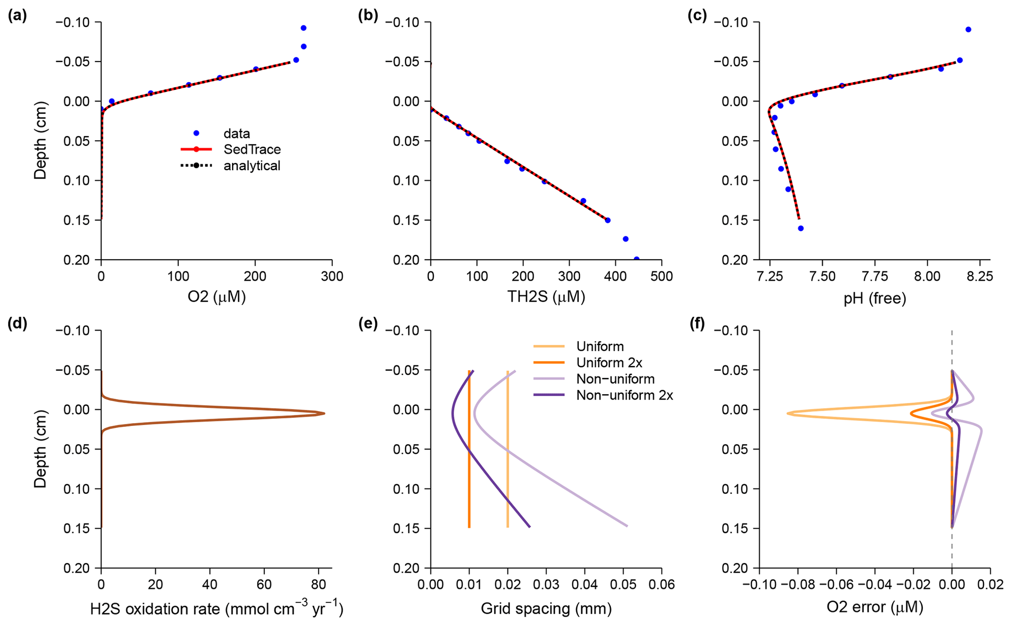
Figure 3 Results of the pHBB1991 model compared with the analytical solution (Boudreau, 1991) and observations (Jørgensen and Revsbech, 1983). (a) Dissolved O₂. (b) Dissolved total H₂S. (c) pH on the free proton scale. (d) Rate of H₂S oxidation by O₂. In panels (a) to (d) the model solutions are computed using the uniform grid with Ngrid = 100. (e) Model grid cell size. (f) Errors of modeled O₂ concentration, defined as the difference between the model solution and the analytical solution. In panels (e) and (f) I show the model solutions on four grids: the uniform grid with Ngrid = 100 and Ngrid = 100 (2×), as well as the nonuniform grid with Ngrid = 100 and Ngrid = 200 (2×).

I tested the sensitivity of the model error (with respect to the analytical solution) to the model grid. I created the model with either a uniform or a nonuniform grid. The gridtran for the uniform grid is simply x->x-0.05, where the 0.05 cm offset is to take into account the fact that SedTrace's internally uniform grid starts from 0 cm. The gridtran for the nonuniform grid is constructed using hyperbolic functions (Hoffmann and Chiang, 2000):

$$\begin{array}{}\text{(54)}& \begin{array}{rl}& \mathtt{\text{gridtran}}\left(x\right)=\left(x_{\mathrm{0}}+\mathrm{0.05}\right)\left(\mathrm{1}+{\displaystyle \frac{\sinh \left(b\left(\frac{x}{L}-A\right)\right)}{\sinh \left(bA\right)}}\right)\\ & -\mathrm{0.05},A={\displaystyle \frac{\mathrm{1}}{\mathrm{2}b}}\ln {\displaystyle \frac{\mathrm{1}+(e^{\mathrm{b}}-\mathrm{1})\left(x_{\mathrm{0}}+\mathrm{0.05}\right)/L}{\mathrm{1}+(e^{-b}-\mathrm{1})(x_{\mathrm{0}}+\mathrm{0.05})/L}},\end{array}\end{array}$$

where L=0.2 cm is the length of the model domain and 0.05 cm is the offset. The resulting grid points are concentrated near x₀=0.005 cm, the degree of which is controlled by b. I tested both types of grid with Ngrid of 100 and 200.

The model results, the analytical solution and the observations made using profiling micro-electrodes are shown in Fig. 3. The nonuniform grid captures the sharp biogeochemical gradient near x₀=0.005 cm better than the uniform grid when Ngrid is the same. The L^∞ norms of the model errors of O₂ are 0.086, 0.021, 0.015 and 0.0039 µM for the uniform grid (Ngrid=100), uniform grid 2X (Ngrid=200), nonuniform grid (Ngrid=100) and uniform grid 2X (Ngrid=200), respectively. Thus, using a suitable grid can considerably improve the model accuracy.

8.2 Oregon margin diagenetic Nd cycle

Neodymium is one of the rare-earth elements (REEs), which are important tracers in chemical oceanography (Elderfield and Greaves, 1982). Its radiogenic isotope composition, expressed as ${\mathit{\epsilon }}_{\mathrm{Nd}}=(\frac{{}^{\mathrm{143}}\mathrm{Nd}/{}^{\mathrm{144}}{\mathrm{Nd}}_{\mathrm{Sample}}}{{}^{\mathrm{143}}\mathrm{Nd}/{}^{\mathrm{144}}{\mathrm{Nd}}_{\mathrm{CHUR}}}-\mathrm{1})\times {\mathrm{10}}^{\mathrm{4}}$ where CHUR is the chondritic uniform reservoir, has been used to study modern and past ocean circulation, as well as marine and continental weathering (Goldstein and Hemming, 2003; Haley et al., 2017; Lacan and Jeandel, 2005; Frank, 2002). It is designated as a “key parameter” by the GEOTRACES program so that it needs to be measured by all affiliated cruises. One of the greatest challenges facing the study of the modern ocean Nd cycle is that its sedimentary cycle is poorly constrained. Recently studies suggest that a benthic flux from marine sediments, particularly in the deep sea, is likely the dominant source of seawater Nd, far exceeding that of riverine and dust inputs at the ocean surface (Abbott et al., 2015b; Du et al., 2018, 2020; Haley et al., 2017). Consequently, pore water ε_Nd, subject to diagenetic processes such as marine silicate weathering, can affect the water column ε_Nd (Abbott et al., 2015a, 2016; Du et al., 2016). Because of the low Nd concentration, ∼1 L of pore water is typically required to make an isotope measurement. Thus, pore water ε_Nd analysis to date has only been done at three sites on the Oregon margin in the northeastern Pacific (Abbott et al., 2016, 2015a). Modeling is needed to make efficient use of the data and extrapolate to other regions once the diagenetic processes are well understood.

Our group recently published a reactive-transport model for the early diagenesis of Nd at a deep-sea site (3000 m water depth) on the Oregon margin (Du et al., 2022), which is regenerated here using SedTrace. This model has 41 kinetic reactions, including the organic matter remineralization sequence, secondary redox reactions, and the diagenesis of carbonate, sulfide and opal. Pore water pH is modeled by including the EIs TCO₂, TH₂S and TH₃BO₃. Aqueous speciation of Fe²⁺ and Al³⁺ is included to model mineral dissolution and precipitation. Adsorption of Fe²⁺ and Mn²⁺ onto Fe and Mn oxides is also included. ¹⁴⁴Nd (Ndnr) and the radiogenic ¹⁴³Nd (Ndr) are modeled as two tracers. The following aqueous- and solid-phase speciation is included for both isotopes: complexation with CO${}_{\mathrm{3}}^{\mathrm{2}-}$, HCO${}_{\mathrm{3}}^{-}$, OH⁻, Cl⁻, SO${}_{\mathrm{4}}^{\mathrm{2}-}$ and H₃SiO${}_{\mathrm{4}}^{-}$; adsorption onto Fe and Mn oxides; incorporation into Fe and Mn oxides by co-precipitation; and formation of the authigenic phosphate mineral rhabdophane, released as trace constituents from primary silicates. By including co-cycling with Fe, Mn and phosphate as well as release by marine silicate weathering coupled to reverse weathering, the model successfully simulated the pore water Nd concentration and ε_Nd data (Fig. 4). This model is relatively large, containing 10 200 equations of 34 model substances on 300 grids between 0 and 50 cm. Interested readers should consult Du et al. (2022) for details of the model description. This model can be found in /examples/OregonNd.

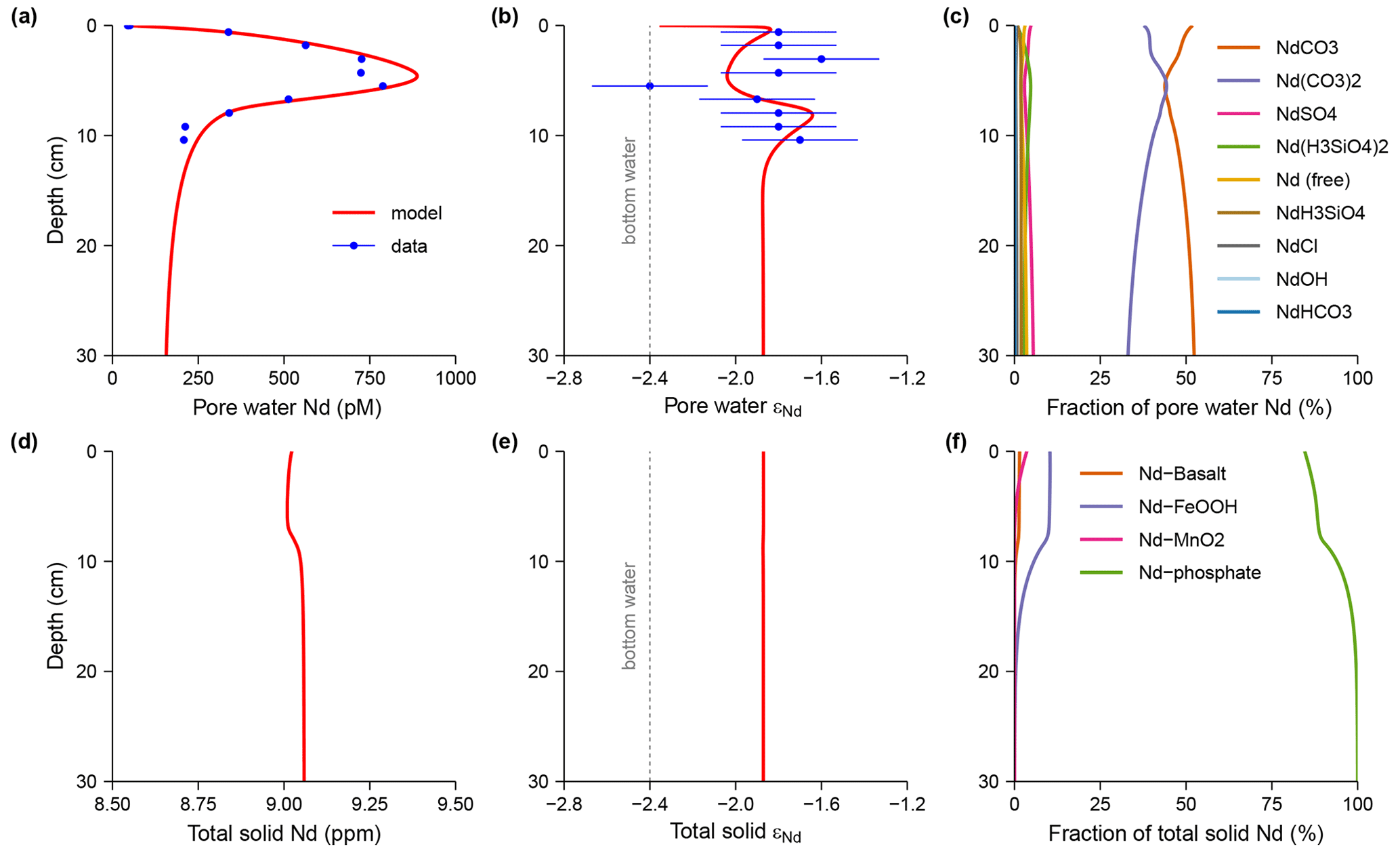
Figure 4 Results of the OregonNd model compared with measurements (Du et al., 2022; Abbott et al., 2015a). (a) Pore water Nd concentration. (b) Pore water ε_Nd. Error bars of the data are 2 standard deviations. (c) Pore water Nd speciation. (d) Total solid Nd, including authigenic Nd associated with Fe and Mn oxides and phosphate as well as lithogenic Nd associated with basalt. This does not include other lithogenic Nd not in the model. (e) Total solid ε_Nd. (f) Solid Nd speciation.

8.3 Santa Barbara Basin sediment biogeochemistry, pH and Mo

Santa Barbara Basin (SBB) is one of the California borderland basins. Its seasonally anoxic condition leads to organic-rich and laminated sediments (Reimers et al., 1996). SBB is among the most studied locations for sediment diagenesis and has perhaps one of the most complete pore water datasets to offer in the literature (Reimers et al., 1996). High-quality pH measurements by in situ profiling micro-electrodes and the availability of various TEI data make it ideal for benchmarking diagenetic models (Meysman et al., 2003). Using SedTrace, I generated a diagenetic model for SBB that includes sediment biogeochemistry, pH and Mo cycling. This example is included in /examples/SBB.

The biogeochemical reaction network includes the classic redox sequence of aerobic respiration, denitrification, Mn and Fe reduction, sulfate reduction, and methanogenesis. The model also includes secondary redox reactions and the authigenesis of carbonates, sulfide, opal and carbonate fluorapatite (CFA). The adsorption of NH${}_{\mathrm{4}}^{+}$, Fe²⁺ and Mn²⁺ is treated using the linear isothermal. To model pH, I include the following equilibrium invariants: TCO₂, TH₂S, THSO₄, TH₃BO₃, TH₃PO₄ and THF. The biogeochemical model includes 26 substances and 36 kinetic reactions. I use a 500-point nonuniform grid with finer spacing close to the SWI. The total number of equations in the biogeochemical model is thus 13 000. Figure 5 shows the modeled sediment biogeochemistry.

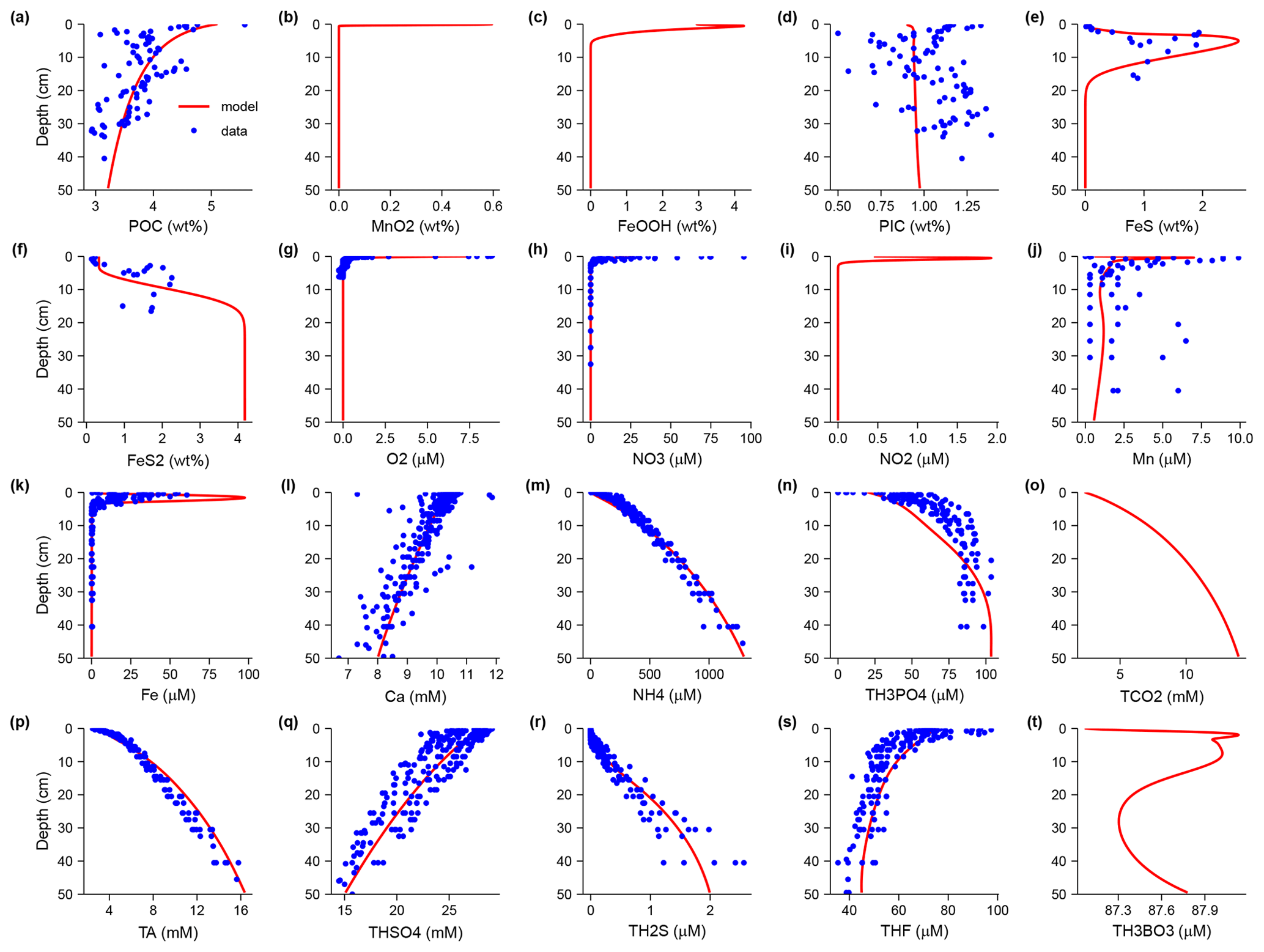
Figure 5 Santa Barbara Basin sediment biogeochemistry. Concentrations of solid sediment substances: (a) particulate organic carbon, (b) Mn oxide, (c) Fe oxide, (d) particulate inorganic carbon, (e) FeS, (f) pyrite. Concentrations of dissolved substances: (g) O₂, (h) NO₃, (i) NO₂, (j) Mn, (k) Fe, (l) Ca, (m) NH₄, (n) total phosphate, (o) total dissolved inorganic carbon, (p) total alkalinity, (q) total sulfate, (r) total sulfide, (s) total fluoride, (t) total boron. Names that begin with the prefix “T” (e.g., TCO₂) indicate equilibrium invariants. Data are from Reimers et al. (1996).

The top 50 cm of the sediment represents ∼150 years of sedimentation. The model successfully reproduced the measurements of pore water constituents, which respond much faster to perturbations of the seasonal cycle and other variabilities, while the solid sediment components show non-steady-state behaviors (Fig. 5). During the sampling time bottom water was low (∼9 µM) but not anoxic, and the oxygen penetration depth was ∼1 cm, below which H₂S is immediately detectable. There was active formation of authigenic minerals (Reimers et al., 1996). Intense Fe cycling leads to high concentrations of FeS and FeS₂. Decreasing pore water Ca concentration is evidence of authigenic carbonate precipitation, and the model shows that Ca, Fe and Mn carbonates are likely formed. Decreasing pore water F concentration and a relatively low PO₄ concentration are explained by CFA precipitation in the model (Jahnke, 1984; Reimers et al., 1996).

The model also captures the measured pH profile (Fig. 6). The pH measurements were reported on the seawater scale, and the model computes pH on this scale by summing the concentrations of free protons, HSO${}_{\mathrm{4}}^{-}$ and HF. Using DSA (Hofmann et al., 2008), the model can easily partition the changes in pH to relevant transport and reaction terms (Fig. 6b–e). The overall increase in pH is driven by Fe reduction in the model (Fig. 6d), as suggested by previous studies (Reimers et al., 1996; Boudreau and Canfield, 1988). This increase in pH is responsible for the saturation and precipitation of authigenic carbonate and CFA. The slight decrease in pH at ∼3.5 cm (Fig. 6a) is modeled by FeS precipitation, which releases protons to pore water (Fig. 6d). The reaction rates of proton are balanced by the transport rate largely attributed to by total alkalinity, TCO₂ and TH₂S (Fig. 6b). This example highlights the capacity of SedTrace for mechanistic studies of what controls pore water pH following the DSA approach in Sect. 4.2.

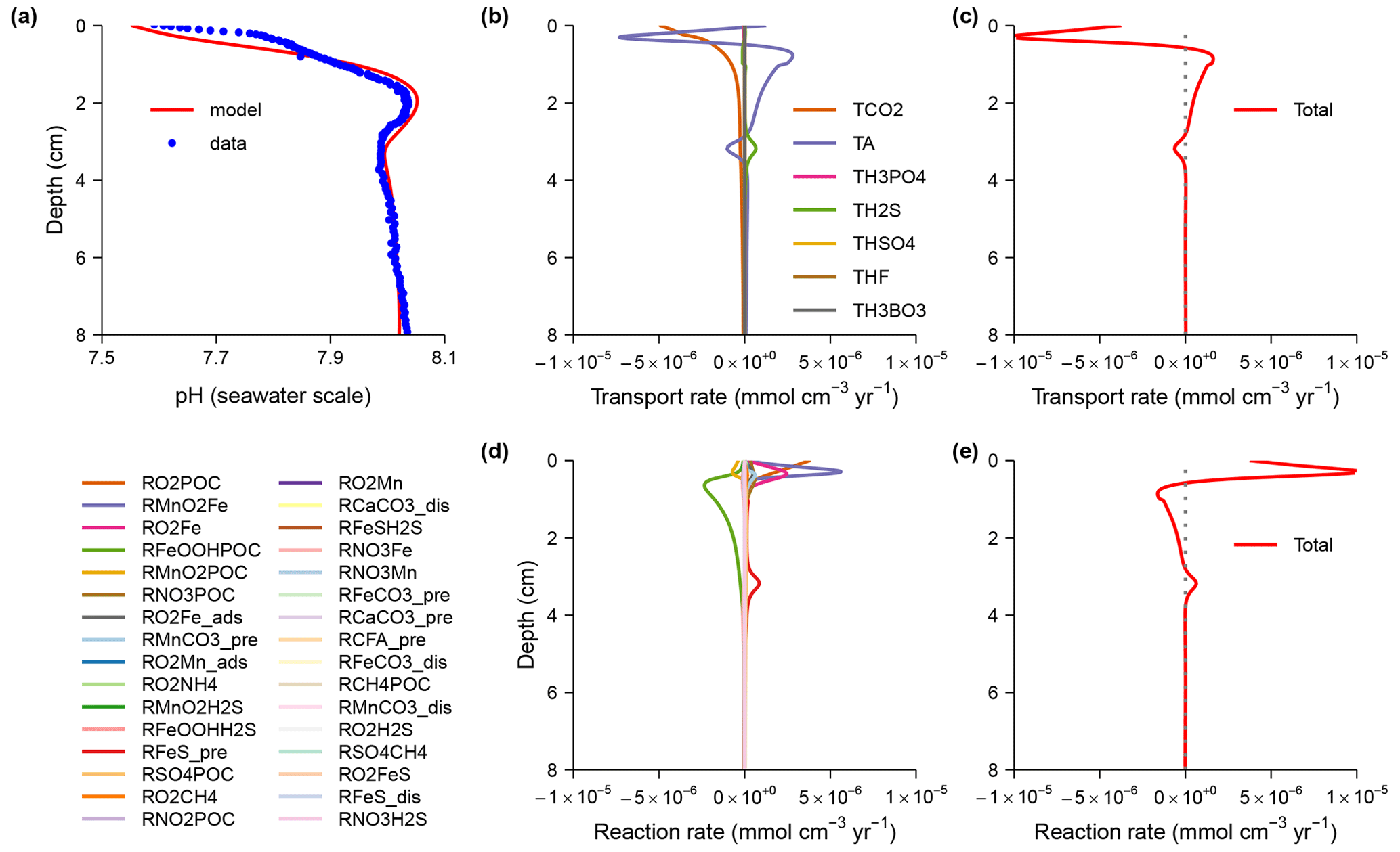
Figure 6 Santa Barbara Basin pore water pH. (a) Modeled pH compared with measured values using in situ profiling micro-electrode probe (Reimers et al., 1996). (b) Rate of [H⁺] change due to the transport of the equilibrium invariants and total alkalinity. (c) The summed transport rate of [H⁺]. (d) Rate of [H⁺] change due to the biogeochemical reactions. Legends is plotted on the left side. Reactions names indicate either redox reactions, such as “RO2POC” in the format of oxidant followed reductant, or mineral dissolution/precipitation reactions with suffix “dis/pre”. (e) The summed reaction rate of [H⁺].

Molybdenum is sensitive to sedimentary redox conditions, and its stable isotope composition, expressed as ${\mathit{\delta }}^{\mathrm{98}}\text{Mo}=(\frac{{}^{\mathrm{98}}\mathrm{Mo}/{}^{\mathrm{95}}{\mathrm{Mo}}_{\mathrm{sample}}}{{}^{\mathrm{98}}\mathrm{Mo}/{}^{\mathrm{95}}{\mathrm{Mo}}_{\mathrm{standard}}}-\mathrm{1})\times {\mathrm{10}}^{\mathrm{3}}+\mathrm{0.25},$ where NIST SRM-3134 is the commonly used standard. Its δ⁹⁸Mo is 0.25 ‰ by convention, which makes it an important proxy to study past ocean deoxygenation (Kendall et al., 2017). SBB provides a useful analogy for an anoxic ocean, and modeling the sedimentary Mo cycle here may help understand how the δ⁹⁸Mo works as a redox proxy. Here I present a test model for Mo diagenesis in SBB to demonstrate the capability of SedTrace to model stable isotope fractionation, complementing the radiogenic isotope example above.

In this model, I consider five dissolved Mo species, MoO${}_{\mathrm{4}}^{\mathrm{2}-}$ and four thiomolybdate species (Erickson and Helz, 2000):

$$\begin{array}{}\text{(55)}& \begin{array}{rl}& {\mathrm{MoO}}_{\mathrm{4}}^{\mathrm{2}-}+i{\mathrm{H}}_{\mathrm{2}}\mathrm{S}={\text{MoO}}_{\mathrm{4}-i}{S}_i^{\mathrm{2}-}+i{\mathrm{H}}_{\mathrm{2}}\mathrm{O}\left(i=\mathrm{1}\text{ to }\mathrm{4}\right),\\ & K_i={\displaystyle \frac{\left[{\text{MoO}}_{\mathrm{4}-i}{S}_i^{\mathrm{2}-}\right]}{\left[{\text{MoO}}_{\mathrm{4}}^{\mathrm{2}-}\right][{\mathrm{H}}_{\mathrm{2}}\mathrm{S}{]}^i}}.\end{array}\end{array}$$

K_i represents the apparent equilibrium constants.

I include ⁹⁸Mo (Moh) and ⁹⁵Mo (Mol) as two tracers. I assume that the equilibrium isotope fractionation is induced during thiolation:

$$\begin{array}{}\text{(56)}& {\mathit{\alpha }}_i^{\mathrm{98}/\mathrm{95}}={\displaystyle \frac{{}^{\mathrm{98}}{\mathrm{MoO}}_{\mathrm{4}}^{\mathrm{2}-}}{{}^{\mathrm{95}}{\mathrm{MoO}}_{\mathrm{4}}^{\mathrm{2}-}}}/{\displaystyle \frac{{{}^{\mathrm{98}}\mathrm{MoO}}_{\mathrm{4}-i}{S}_i^{\mathrm{2}-}}{{{}^{\mathrm{95}}\mathrm{MoO}}_{\mathrm{4}-i}{S}_i^{\mathrm{2}-}}}=K_i^{\mathrm{98}}/K_i^{\mathrm{95}},\end{array}$$

where ${\mathit{\alpha }}_i^{\mathrm{98}/\mathrm{95}}$ represents the fractionation factors, which are 1.0014, 1.0028, 1.00455 and 1.0063 (or 1.40 ‰, 2.80 ‰, 4.54 ‰ and 6.28 ‰, respectively, in the δ notation) for i=1 to 4 respectively estimated by ab initio calculation (Tossell, 2005) and recalculated by Kendall et al. (2017). In SedTrace, I add Eq. (55) to the speciation sheet, choosing MoO${}_{\mathrm{4}}^{\mathrm{2}-}$ as the base species. Presently SedTrace does not provide special treatment of isotope fractionation, so the user needs to incorporate the fractionation factor in the parameters (e.g., K_i) before supplying them to SedTrace. I use the constants from Erickson and Helz (2000) as $K_i^{\mathrm{95}}$ and then multiply them by ${\mathit{\alpha }}_i^{\mathrm{98}/\mathrm{95}}$ to get $K_i^{\mathrm{98}}$.

I test the model sensitivity to the Mo removal mechanism. In Case 1, I assume all thiomolybdate species can be removed by scavenging:

$$\begin{array}{}\text{(57)}& {\mathrm{RMo}}_{\mathrm{rm}\mathrm{1}}=k_{\mathrm{rm}\mathrm{1}}\sum _i\left[{\text{MoO}}_{\mathrm{4}-i}{S}_i^{\mathrm{2}-}\right].\end{array}$$

In Case 2 I assume that only tetrathiomolybdate can be removed by scavenging:

$$\begin{array}{}\text{(58)}& {\mathrm{RMo}}_{\mathrm{rm}\mathrm{2}}=k_{\mathrm{rm}\mathrm{2}}\left[{\mathrm{MoS}}_{\mathrm{4}}^{\mathrm{2}-}\right].\end{array}$$

In this test I do not consider kinetic isotope fractionation during removal and diffusion, and reactions in Eq. (55) are assumed to be fast enough to reach local equilibrium. In Eq. (57) I assume all species are removed at the same rate constant. I assume the bottom-water δ⁹⁸Mo to be the same as the seawater, which is globally uniform at 2.34 ‰ (Kendall et al., 2017). The only source of authigenic Mo accumulation is pore water Mo removal supported by diffusion of seawater into sediment. In the model I also supply a lithogenic Mo flux to account for the reported 2 ppm lithogenic Mo in sediments (Zheng et al., 2000). The lithogenic δ⁹⁸Mo is assumed to be the same as the upper continental crust (UCC) of ∼0.3 ‰ (Kendall et al., 2017).

In SedTrace I further add six Mo tracers to the biogeochemical model described above, including the two Mo isotopes in pore water, as well as lithogenic and authigenic fractions, increasing the total number of model equations to 16 000.

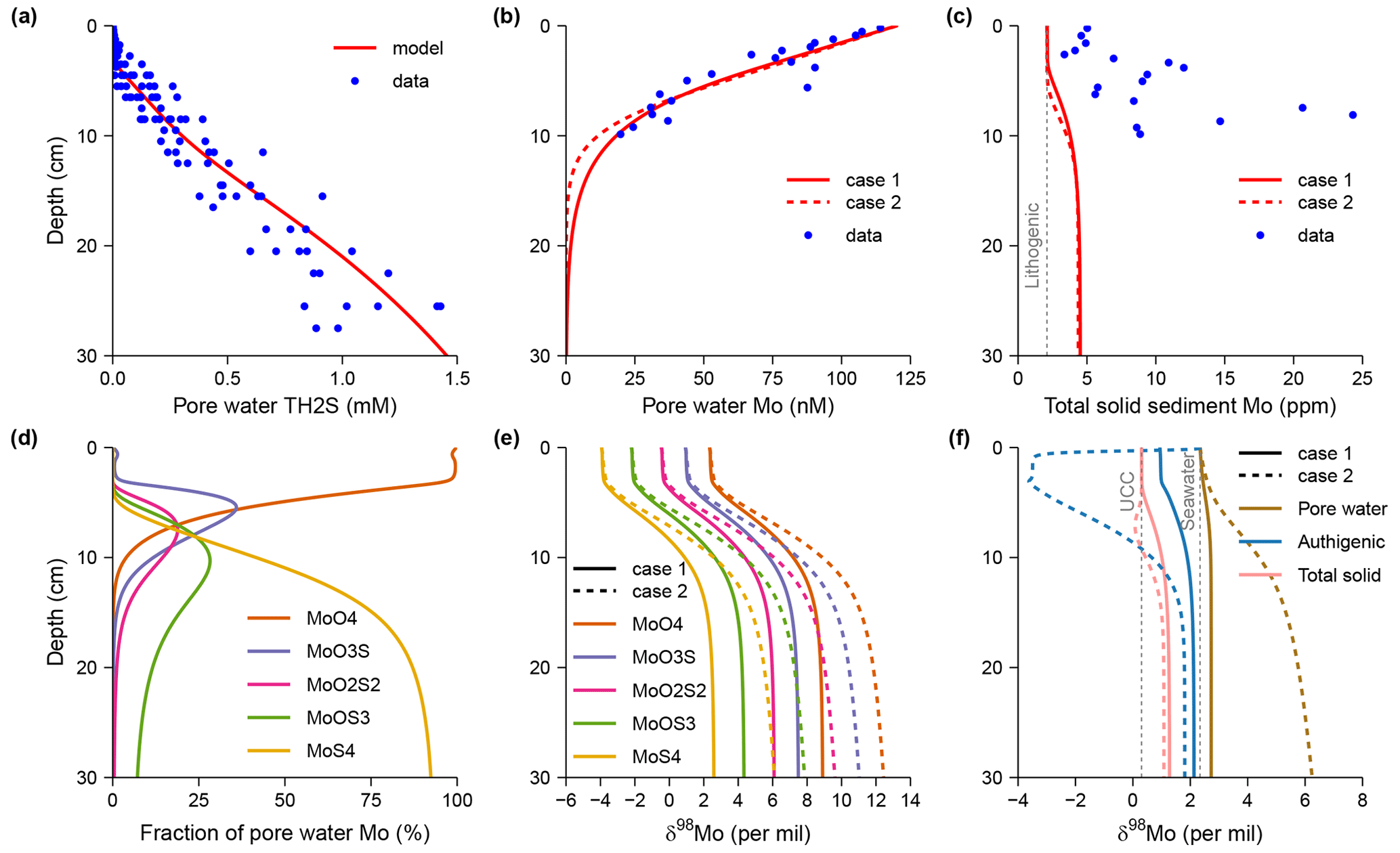
Figure 7 Santa Barbara Basin sediment Mo cycle. (a) Modeled and measured total sulfide (Reimers et al., 1996). (b) Modeled and measured pore water Mo (Zheng et al., 2000). (c) Modeled and measured total solid sediment Mo (Zheng et al., 2000). (d) Modeled pore water Mo speciation. (e) Modeled δ⁹⁸Mo of the dissolved species. (f) Modeled δ⁹⁸Mo of pore water, authigenic and total solid sediment.

In the two model cases I vary k_rm1 and k_rm2 to fit the measured pore water Mo concentration profile (Fig. 7b) (Zheng et al., 2000). The model results of the two cases are roughly the same. As H₂S concentration increases, pore water Mo speciation is dominated by the thiomolybdate species (Fig. 7d). The aqueous speciation in the two cases is identical since it only depends on the concentration of H₂S. The modeled total solid (sum of authigenic and lithogenic) sediment Mo concentrations in the two cases are also similar, but both are much lower than measured (Fig. 7c) (Zheng et al., 2000). Modeled authigenic Mo enrichments, relative to the 2 ppm lithogenic background, do not start until below ∼5 cm. The model results suggest that the Mo diffusion and removal rate at the time of pore water sampling cannot explain the history of sediment Mo enrichment in the top 10 cm. Non-steady-state accumulation and other Mo sources, such as Mo carried into sediments by settling particles, are needed to close the sedimentary budget (Zheng et al., 2000).

Modeled thiomolybdate species all have lighter δ⁹⁸Mo than MoO${}_{\mathrm{4}}^{\mathrm{2}-}$ (Fig. 7e). The removal of thiomolybdate thus makes the residual pore water δ⁹⁸Mo heavier than seawater (Fig. 7f). In Case 1 where all thiomolybdate species are removed, the apparent fractionation between pore water and authigenic sediment (<1.4 ‰) is much smaller than in Case 2 where only tetrathiomolybdate is removed (as much as 6.5 ‰). In contrast, the δ⁹⁸Mo of total sediment has little sensitivity to the removal mechanism (Fig. 7f). This illustrates the underappreciated challenge of applying detrital corrections to TEI data: the most useful data to differentiate the removal mechanism in this test are the authigenic δ⁹⁸Mo at near-zero authigenic enrichment, which unfortunately will have the greatest uncertainty when applying detrital correction in reality (Ciscato et al., 2018).

As pore water Mo removal becomes quantitative below 25 cm, authigenic δ⁹⁸Mo approaches the seawater δ⁹⁸Mo. However, unlike in a closed system, modeled authigenic δ⁹⁸Mo never reaches the seawater value even at depths of quantitative removal. This is because in a reactive-transport system, the memory of the authigenic enrichment of light Mo isotope in the zone of partial removal will persist.

9 Future developments

Future developments of SedTrace will improve the user interface, the speciation modeling capacity and parameter selection. Currently SedTrace has no specialized interface for isotopes, and the user needs to add the isotopes as individual tracers and supply parameters that already incorporate the stable isotope fractionation factor and radiogenic isotope source. A more user-friendly interface for modeling isotopes is planned. Also, the current implementation of adsorption and aqueous speciation can be further improved to allow more flexible and mechanistic formulations of speciation: for example, including the speciation of dissolved and surface ligands. At the moment, SedTrace only precomputes selected parameters such as diffusion coefficients and acid dissociation constants, while it requires the user to supply the rest. Integration with the Miami ion interaction model for seawater (Pierrot and Millero, 2017) and the Pitzer-equation-based seawater speciation model being developed by the SCOR working group (Humphreys et al., 2022) would allow SedTrace to precompute more parameters and lessen the burden on the user.

Future developments will also aim to add more choices of numerical methods and improve numerical performance. Currently SedTrace only uses CVODE with the iterative method of solving linear systems (Hindmarsh et al., 2005; Gardner et al., 2022). Although I have found it to be more efficient when solving a large stiff system of equations, in other cases other ODE solvers or the direct method of solving linear systems may be preferable. Further release will enhance the integration of SedTrace with DifferentialEquations.jl (Rackauckas and Nie, 2017) and provide the user with more numerical choices. Similarly, more options of preconditioners can also be added. Also, SedTrace currently has no parallel computing capacity (aside from those done internally by Julia), and model simulation cannot take advantage of the multicore architecture of modern computers. Future development will focus on enabling SedTrace for parallel computing, for example, through integration with the PETSc.jl package, the Julia interface for the Portable, Extensible Toolkit for Scientific Computation system that uses the Messaging Passing Interface (MPI) for a scalable solution of differential equations (Balay et al., 2022). Such high performance is needed if SedTrace is to be used to solve global-scale problems.

Currently SedTrace's capacity is limited to the forward modeling of steady-state diagenesis. A special interface can be added to enable the user to add time-dependent forcing in parameters or boundary conditions for fully transient modeling. Moreover, since SedTrace already enables automatic differentiation, capacities of adjoint sensitivity analysis, parameter estimation, inverse modeling and data assimilation can be added by integration with relevant existing Julia packages (Rackauckas and Nie, 2017; Dunning et al., 2017).