A new model for supraglacial hydrology evolution and drainage for the Greenland Ice Sheet (SHED v1.0)

The Greenland Ice Sheet (GrIS) is losing mass as the climate warms through both increased meltwater runoff and ice discharge at marine-terminating sectors. At the ice sheet surface, meltwater runoff forms a dynamic supraglacial hydrological system which includes stream and river networks and large supraglacial lakes (SGLs). Streams and rivers can route water into crevasses or into supraglacial lakes with crevasses underneath, both of which can then hydrofracture to the ice sheet base, providing a mechanism for the surface meltwater to access the bed. Understanding where, when, and how much meltwater is transferred to the bed is important because variability in meltwater supply to the bed can increase ice flow speeds, potentially impacting the hypsometry of the ice sheet in grounded sectors, and iceberg discharge to the ocean. Here we present a new, physically based, supraglacial hydrology model for the GrIS that is able to simulate (a) surface meltwater routing and SGL filling; (b) rapid meltwater drainage to the ice sheet bed via the hydrofracture of surface crevasses both in and outside of SGLs; (c) slow SGL drainage via overflow in supraglacial meltwater channels; and, by offline coupling with a second model, (d) the freezing and unfreezing of SGLs from autumn to spring. We call the model the Supraglacial Hydrology Evolution and Drainage (or SHED) model. We apply the model to three study regions in southwest Greenland between 2015 and 2019 (inclusive) and evaluate its performance with respect to observed supraglacial lake extents and proglacial discharge measurements. We show that the model reproduces 80 % of observed lake locations and provides good agreement with observations in terms of the temporal evolution of lake extent. Modelled moulin density values are in keeping with those previously published, and seasonal and inter-annual variability in proglacial discharge agrees well with that which is observed, though the observations lag the model by a few days since they include transit time through the subglacial system, while the model does not. Our simulations suggest that lake drainage behaviours may be more complex than traditional models suggest, with lakes in our model draining through a combination of both overflow and hydrofracture and with some lakes draining only partially and then refreezing. This suggests that, in order to simulate the evolution of Greenland's surface hydrological system with fidelity, a model that includes all of these processes needs to be used. In future work, we will couple our model to a subglacial model and an ice flow model and thus use our estimates of where, when, and how much meltwater gets to the bed to understand the consequences for ice flow.

1 Introduction

The Greenland Ice Sheet (GrIS) is losing mass at an accelerated rate. For example, the contribution of the GrIS to global sea level rise was 0.29 ± 0.02 mm a⁻¹ between 1972 and 2018 (Mouginot et al., 2019) but 1.27 mm a⁻¹ between 2013 and 2019 (Smith et al., 2020), a 4-fold increase. This is projected to continue as the climate warms further, and the GrIS is expected to be a major contributor to global sea level rise for at least the rest of this century (e.g. Mouginot et al., 2019; Smith et al., 2020).

GrIS mass loss is attributed to an imbalance between mass gain due to snowfall and mass loss due to surface melting and dynamic ice discharge (The IMBIE Team, 2020). Ice flow dynamics are complex and governed by a number of interconnected processes, such as the effect of meltwater transfer from the ice sheet's surface to its bed on subglacial water pressure (e.g. Banwell et al., 2013, 2016; Christoffersen et al., 2018; Schoof, 2010), which can cause significant changes in an ice sheet's seasonal flow speed (e.g. Das et al. 2008; Tedesco et al., 2013). Surface meltwater can reach the ice sheet bed when it either (a) flows into a crevasse (e.g. Clason et al., 2012; van der Veen, 2008) or (b) flows into surface depressions where it ponds to form supraglacial lakes (SGLs) (Leeson et al., 2012; Banwell et al., 2012a), underneath which a crevasse forms (Das et al., 2008) or an existing crevasse is advected into the lake basin from upglacier (e.g. Krawczynski et al., 2009). If a sufficient amount of meltwater accumulates, these crevasses may propagate vertically downwards through the full thickness of the ice (“hydrofracture”, van der Veen, 2008), draining the meltwater to the bed and, in the case of an SGL, draining the rest of the lake. Ultimately this may result in the formation of a moulin (Tedesco et al., 2013), which is likely to stay open for the remainder of the melt season (Banwell et al., 2016). The routing of meltwater to the ice sheet's bed may increase the subglacial water pressure, which, in turn, increases local basal lubrication. This provides a mechanism by which seasonal variations in the production of surface runoff can strongly affect variations in ice flow velocities (e.g. Zwally et al., 2002). Indeed, hydrofracture-induced lake drainage events have been observed to accelerate ice flow up to 140 km inland from the ice sheet margin (Doyle et al., 2014).

Studies have shown that the SGLs on the GrIS start to form in late May and increase in number and area as the melt season progresses (e.g. Fitzpatrick et al., 2014; Williamson et al., 2018a; Selmes et al., 2011). In addition to draining vertically, SGLs may also drain laterally by means of overflowing and potential channel incision (e.g. Tedesco et al., 2013). This water may then be routed across the ice sheet to other SGLs or to existing crevasses and moulins and ultimately into the subglacial environment (e.g. Kingslake et al., 2015; Banwell et al., 2016). The SGLs that either do not or only partially drain during the melt season refreeze over winter, either fully or partially, following the development of an ice lid that insulates the water beneath from the sub-freezing air temperatures (e.g. Law et al., 2020). Refrozen lakes act as a store of surface meltwater over winter, and they unfreeze the following spring, when they can accumulate more water and then potentially drain.

These hydrological processes are complex and interconnected and are not all fully accounted for in any ice sheet hydrology model to date. Past supraglacial meltwater modelling studies have incorporated one or more of the following: (i) rapid SGL drainage parameterized as a function of lake volume (e.g. Banwell et al., 2013, 2016); (ii) rapid SGL drainage through physically based process representation, e.g. via hydrofracture using linear elastic fracture mechanics (LEFM) combined with knowledge of the ice sheet stress field (e.g. Hoffman et al., 2018; Koziol et al., 2017; Clason et al., 2012, 2015); (iii) slow SGL drainage via overflow using a simple sheet flow mechanism (e.g. Leeson et al., 2012; Banwell et al., 2013); (iv) slow SGL drainage via supraglacial meltwater channel incision (Hill and Dow, 2021; Koziol et al., 2017); and (v) SGL refreezing (e.g. Buzzard et al., 2017; Law et al., 2020).

Here, we present a new, high-spatial-resolution (100 m), physically based supraglacial hydrology model that is able to model SGL formation and growth, overflow and lateral drainage, drainage by hydrofracture, and freezing and unfreezing. Furthermore, our model also simulates hydrofracture and moulin creation through crevasses occurring outside of lakes. The model builds on that of Leeson et al. (2012) by adding additional components to simulate (i) the rapid drainage of SGLs by hydrofracture using LEFM combined with the ice sheet stress field (e.g. Clason et al., 2015) and (ii) the slow drainage of SGLs through overflow and the incision of supraglacial streams (e.g. Kingslake et al., 2015). We also include an offline coupling with a lake-refreezing model (e.g. Buzzard et al., 2017; Law et al., 2020). We show that our model is able to simulate these processes with reasonable fidelity, and we present initial findings based on simulations performed using the model.

2 Study areas

To calibrate and validate our model, we perform simulations across three study regions in the southwest GrIS (Fig. 1): region 1, region 2, and region 3. Three study regions were chosen since the supraglacial hydrological network evolves differently in each region, and different amounts of data with which to force and evaluate our model are available in each (Table 1).

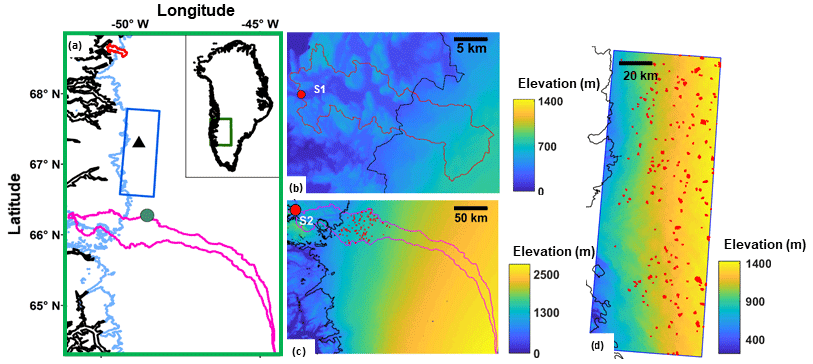
Figure 1 (a) Locations of the three study regions in southwest Greenland – region 1 (red outline), region 2 (pink outline), and region 3 (blue box) – where our supraglacial hydrology model was applied. The thick black line represents the coastline. The light-blue line represents the ice margin. The green dot in region 2 represents the SGL discussed in Sect. 5.3 and shown in Fig. 8. The black triangle in region 3 represents the SGL discussed in Sect. 5.5 and shown in Fig. 10. (b) The basin boundaries for region 1 are overlaid onto the respective surface DEM data. The hydrological basin boundary is represented by a red line. The location of the Kuussuup proglacial gauging station (S1) is shown by a red dot. The ice margin is represented by a solid black line. (c) The basin boundaries for region 2 are overlaid onto the respective surface DEM data. The hydrological basin boundary is represented by a pink colour. The location of the Tasersiaq proglacial gauging station (S2) is shown by a red dot. The ice margin is represented by a solid black line. The red features inside the basin represent the observed maximum extents of the SGLs that formed in 2019. (d) The basin boundaries for region 3 are overlaid onto the respective surface DEM data. The hydrological basin boundary is represented by a blue line. There is no proglacial gauging station for region 3. The ice margin is represented by a solid black line. The red features inside the basin represent the observed maximum extents of the SGLs that formed in 2015, 2016, 2017, and 2018.

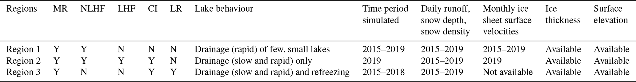
Table 1 Model components tested in each of the three regions and the time period of model runs. The abbreviations are as follows: MR – meltwater routing, NLHF – non-lake hydrofracture, LHF – lake hydrofracture, CI – channel incision, LR – lake refreezing, Y – yes, and N – no. The column labelled “Time period simulated” represents the duration for which the hydrological model was run over each of the regions. The column labelled “Lake behaviour” describes the characteristics of the lakes that the model aims to simulate. The rest of the columns to the right of “Time period simulated” show the availability of forcing data for each region between 2015 and 2019 (inclusive), including ice velocity, MAR data, surface elevation, and ice thickness.

Region 1 is a single hydrological catchment covering a total area of ∼ 221 km², of which ∼ 95 km² (42 %) is covered by the ice sheet with a maximum ice thickness of ∼ 680 m (Fig. 1). The region is entirely within 3 km of the ice sheet margin and appears to be heavily crevassed in optical satellite imagery, which means it has very few and very small SGLs. Instead, meltwater appears to generally be routed into the englacial system via crevasses before it is able to pond on the surface. The model was run for this study area over the period 2015 to 2019, and results are compared against proglacial discharge data acquired at gauging station S1 (Table 1).

Region 2 is also a single hydrological catchment, but it spans a larger area than region 1 – specifically 8166 km², of which ∼ 6117 km² (∼ 75 %) is covered by the ice sheet, with a maximum ice thickness of 2500 m. Over 100 SGLs form in this region each summer (Fig. 1), and the majority of them appear to drain by the end of the melt season (with none refreezing) according to optical satellite imagery. In region 2, the model was run for 2019 only due to a paucity of ice flow data needed to force the model (Table 1). Simulations performed for region 2 are used to calibrate the model and to validate the lake drainage processes included in our model, i.e. rapid drainage by hydrofracture and slow drainage by overflow and channel incision. MODIS-based observations of lake area (see Sect. 3) and proglacial discharge data acquired at gauging station S2 are used to validate these processes.

Region 3 has an area of ∼ 8250 km², of which ∼ 7244 km² (∼ 88 %) is covered by the ice sheet, with a maximum ice thickness of 1500 m (Fig. 1d). Unlike region 1 and region 2, region 3 is not a single hydrological catchment. In this region, optical satellite imagery shows that there are many SGLs that persist throughout the melt season and refreeze in the following winter. This allows us to calibrate and validate the lake-refreezing processes in our model. We note that we are not able to simulate hydrofracture in this region, associated with lakes or not, due to a lack of forcing data (Table 1).

3 Data and methods

Our model requires surface elevation data for routing and ponding of meltwater over the ice sheet. Here we use the 100 m ArcticDEM digital elevation model (DEM) for this purpose, which is derived from in-track and cross-track high-spatial-resolution optical imagery obtained via the Digital Globe Satellite Constellation (Porter et al., 2018). The mean vertical accuracy of the ArcticDEM at a spatial resolution of 2 m is estimated to be −0.01 ± 0.07 m (Candela et al., 2017). We smoothed the DEM using a three-by-three moving kernel to remove relic non-lake features such as supraglacial channels incised in the years prior to the acquisition of the data used to create the DEM.

Climate forcing over regions 1, 2, and 3, specifically daily estimates of surface runoff, snow depth, and snow density, were derived from the MAR v3.11 (Modele Atmospherique Regionale) regional climate model (Amory et al., 2021; Fettweis et al., 2008, 2020), run at 6 km resolution and with lateral boundary forcing provided by the European Centre for Medium-Range Weather Forecasts ERA-5 reanalysis (Hersbach et al., 2020). To simulate lake refreezing over region 3, we also used MAR-derived daily shortwave radiation, air temperature, relative humidity, wind velocity, and cloud cover.

For estimates of ice surface stress fields, we used monthly surface velocity data from Making Earth System Data Records for Use in Research Environments (MEaSUREs; Joughin et al., 2018).

One way in which we calibrate our model is by comparing daily modelled SGL extents with daily SGL extents observed from MODIS Terra 250 m surface reflectance image mosaics (MOD09GQ) (e.g. Lea et al., 2022). Lake margins for each day were automatically extracted following dynamic thresholding of the red band, which previously proved to be successful in identifying rapid changes in SGL extents (Selmes et al., 2011; Williamson et al., 2018a). To reduce false positives in the daily SGL records, all lakes identified were (a) ≥ 3 km from the ice margin (to avoid rock outcrops or sediment being falsely identified as SGLs where the image analysis kernel overlaps with the ice margin), (b) had an area > 0.125 km² (i.e. two MODIS grid cells), (c) appeared ≥ 2 times within a 6 d window run throughout the melt season, and (d) appeared in images with < 80 % cloud cover (following Cooley and Christoffersen, 2017). We note that we filtered our modelled lakes to remove lakes smaller than 13 DEM pixels (0.125 km²) in our comparison of daily SGL area observed by MODIS and that simulated using our model (Fig. 6).

To evaluate our modelled proglacial discharge (i.e. the sum of supraglacial runoff and discharge through lake and non-lake crevasses and moulins) for both region 1 and region 2, we use daily in situ proglacial discharge data measured at the ice sheet margin by the Asiaq Greenland Survey (AGS). AGS produced these data by first subtracting the runoff contribution from land (e.g. predominantly from rainfall) from the measured proglacial discharge data before the remaining proglacial discharge was then adjusted for the routing delay over land between the ice sheet margin and the proglacial gauging station.

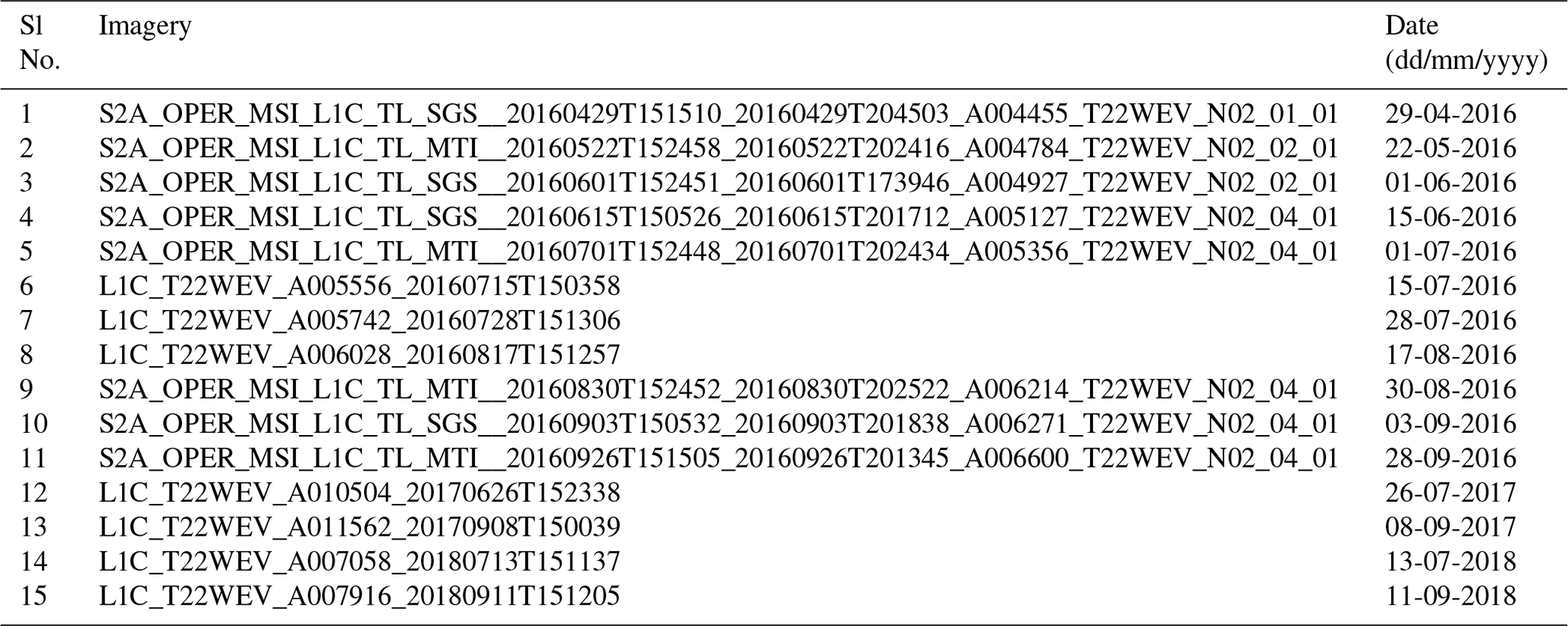
To evaluate lake freezing and unfreezing in our model, we visually compare our modelled output for a refreezing lake with the corresponding observations from Sentinel-2 imagery acquired in the spring and summer for the period between 2015 and 2018. A complete list of images used is given in Table A1 in the Appendix.

4 Model description

Our supraglacial hydrology model is run at 100 m spatial resolution and daily temporal resolution. We appreciate that some lakes drain rapidly by means of hydrofracture on sub-daily timescales (e.g. Das et al., 2008; Tedesco et al., 2013); however, sensitivity runs suggested that our results were not significantly different when a finer time step was used. This daily time step also facilitates coupling with a dynamic ice sheet model, which typically runs on much coarser time steps and which we intend to pursue in future work. We note that daily time stepping has also been used by previous studies, e.g. Clason et al. (2012, 2015). Our model comprises four modules: (1) supraglacial routing and lake filling, (2) hydrofracture, (3) slow lake drainage, and (4) lake refreezing (Fig. 2). These components are described in more detail below and in Fig. 2.

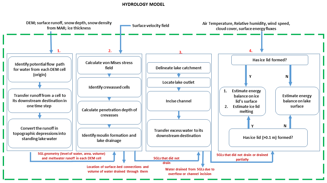
Figure 2 Model schematic. The model includes four main modules, each describing a hydrological process: (1) the surface-routing and lake-filling module, (2) the hydrofracture module; (3) the slow-lake-drainage module; and (4) the lake-refreezing module. The modules are labelled 1, 2, 3, and 4, respectively. Y and N stand for Yes and No respectively.

4.1 Supraglacial-routing and lake-filling module

This module is responsible for routing supraglacial meltwater runoff from an origin DEM cell to a destination DEM cell. The origin cell is either a non-crevassed or a crevassed cell. The destination cell can be crevassed; non-crevassed; or a surface depression called a sink, where meltwater ponds to form an SGL. To simulate the formation and growth of SGLs, we adopt a methodology that is based on the ideas proposed by Arnold et al. (1998) and Arnold (2010) and subsequently used by Banwell et al. (2012a) and which is well suited to coarse time stepping. Following that, in every time step, for every DEM cell, we identify a potential destination cell (PDC) – i.e. the crevassed cell or sink in which water flow from the DEM cell will eventually terminate (see Appendix B). Next, we identify the flow path that the meltwater from a DEM cell would take enroute to its PDC (see Appendix B). Once the flow path is identified, for each pair of cells lying along the flow path, we estimate the corresponding travel time that the meltwater would take while flowing along the flow path. This travel time depends on the meltwater discharge between the pair of cells, which is estimated by either Manning's equation for open-channel flow (Manning, 1891) or by Colbeck's equation for flow through a porous medium (i.e. snow or firn) (Colbeck, 1978) depending on the absence or presence of a snowpack on the ice sheet surface (after Leeson et al., 2012). By integrating the travel times downslope along the flow path, we determine the total time taken by meltwater to flow from a DEM cell to its corresponding PDC. Using this information, the water from each DEM origin cell (the contents of the cell at the start of the day and the daily melt increment produced in the cell) is added to the appropriate cell along the flow path, i.e. the point at which integrated travel time equals 1 d. Where the PDC also represents a sink (i.e. a surface depression), the accumulated water in every time step is used to fill up the sink (see Appendix B), as a result of which an SGL is formed.

4.2 Hydrofracture module

This module simulates the phenomenon of hydraulically driven fracture propagation, i.e. hydrofracture (van der Veen, 2008), and is activated when surface meltwater runoff is routed into either (a) an existing crevasse away from an SGL or (b) a crevasse in an SGL, which either may have been advected into the lake basin or may have opened within the basin during a melt season. For both cases, as meltwater accumulates in a crevasse, the water pressure in the crevasse increases. When this water pressure exceeds the sum of surface tensile strength and the lithostatic stress of the ice, it drives the crevasse vertically down through the ice (e.g. van der Veen, 2008). Once the depth of the crevasse equals the local ice thickness (i.e. when the crevasse reaches the ice sheet bed), the water in the crevasse is assumed to be injected into the subglacial environment, and the crevasse is assumed to remain open in the form of a moulin for the remainder of the melt season (Banwell et al., 2016).

The process of hydrofracture is simulated using the concepts of LEFM (e.g. van der Veen, 2008; Vaughan, 1993; Hoffman et al., 2018; Clason et al., 2012, 2015). In every time step, the surface tensile stress (R_xx) is estimated from the square of the von Mises stress field (${\mathit{\sigma }}_{\mathrm{v}}^{\mathrm{2}}$) that is in turn calculated using Eqs. (1)–(4), as shown below:

$$\begin{array}{}\text{(1)}& {\mathit{\sigma }}_{\mathrm{v}}^{\mathrm{2}}={\mathit{\sigma }}_{\mathrm{1}}{\mathit{\sigma }}_{\mathrm{1}}+{\mathit{\sigma }}_{\mathrm{3}}{\mathit{\sigma }}_{\mathrm{3}}-{\mathit{\sigma }}_{\mathrm{1}}{\mathit{\sigma }}_{\mathrm{3}},\end{array}$$

where σ₁ and σ₃ are the principal stresses which are calculated as follows:

$$\begin{array}{}\text{(2)}& {\displaystyle }{\mathit{\sigma }}_{\mathrm{1}}={\displaystyle \frac{\mathrm{1}}{\mathrm{2}}}\left({\mathit{\sigma }}_{xx}+{\mathit{\sigma }}_{yy}\right)+\sqrt{{\left[{\displaystyle \frac{\mathrm{1}}{\mathrm{2}}}({\mathit{\sigma }}_{xx}+{\mathit{\sigma }}_{yy})\right]}^{\mathrm{2}}+{\mathit{\tau }}_{xy}^{\mathrm{2}}},\text{(3)}& {\displaystyle }{\mathit{\sigma }}_{\mathrm{3}}={\displaystyle \frac{\mathrm{1}}{\mathrm{2}}}\left({\mathit{\sigma }}_{xx}+{\mathit{\sigma }}_{yy}\right)-\sqrt{{\left[{\displaystyle \frac{\mathrm{1}}{\mathrm{2}}}({\mathit{\sigma }}_{xx}+{\mathit{\sigma }}_{yy})\right]}^{\mathrm{2}}+{\mathit{\tau }}_{xy}^{\mathrm{2}}},\end{array}$$

where σ_xx, σ_yy, and τ_xy are longitudinal, lateral, and shear stresses, respectively, and are calculated from the surface velocity field (e.g. Clason et al., 2012, 2015). R_xx is calculated as follows:

$$\begin{array}{}\text{(4)}& R_{xx}=\sqrt{{\mathit{\sigma }}_{\mathrm{v}}^{\mathrm{2}}}.\end{array}$$

All the DEM cells with R_xx greater than the threshold tensile strength of ice (τ_c) are classified as crevassed cells with an initial vertical crevasse depth of 0.1 m (e.g. Clason et al., 2015) and constant width w_c of 0.6 m (see Sect. 5).

For region 1 and region 2, to constrain the values of τ_c and w_c, we ran the model using a range of values of τ_c and w_c on a trial-and-error basis. For τ_c, the values were chosen from the range 200–300 kPa (e.g. Clason et al., 2012, 2015), and the values for w_c were chosen from the range 0.02–2 m (e.g. Krawczynski et al., 2009). Whichever pair of values gave the best match between (a) modelled and observed lake extents and (b) annual modelled discharge and annual measured proglacial discharge was chosen. The results of this calibration are shown in Sect. 5.1.

For crevasses that do not occur beneath an SGL, in every time step, the penetration depth of individual water-filled crevasse cells is calculated by estimating the net stress intensity factor (K_I) following van der Veen (2008):

$$\begin{array}{}\text{(5)}& K_{\mathrm{I}}=\mathrm{1.12}{R}_{xx}\sqrt{\mathit{\pi }d}-\mathrm{0.683}{\mathit{\rho }}_{\mathrm{i}}g{d}^{\mathrm{1.5}}+\mathrm{0.683}g{b}^{\mathrm{1.5}},\end{array}$$

where d is the crevasse depth initialized to 0.1 m; ρ_i is the density of ice; b is the water depth in the crevasse in metres, which is controlled by the crevasse width and depth and the meltwater supply; and g is 9.8 m s⁻². The three terms on the right-hand side of Eq. (5) describe the stress intensity factors relating to the tensile stress, the lithostatic stress of ice, and water filling in the crevasse, respectively. Equation (5) is solved for every crevassed cell at every time step until K_I is less than or equal to the prescribed ice fracture toughness (K_IC), which is assumed to be 150 kPa m^0.5 (e.g. Fischer et al., 1995; Rist et al., 1999). For K_I>=K_IC, d will increase as the water is able to propagate the crevasse vertically down through the ice thickness. As a result, the value of d is increased until K_I<K_IC. When the crevasse depth equals ice thickness (i.e. when it reaches the ice sheet bed), the water is drained in a single time step, which is 1 d in our model (e.g. Clason et al., 2012, 2015).

For crevassed cell(s) occurring underneath a lake, a slightly different procedure was used to simulate hydrofracture. Instead of calculating crevasse propagation depth in every time step (i.e. as we do for crevasses outside of SGLs), we followed the methodology adopted by Clason et al. (2012). First, in every time step, we locate the deepest cell within an SGL. Next, for this one cell, Eq. (5) is solved by first equating the crevasse depth (d) at the time of SGL drainage to the local ice thickness, and the crevasse water depth (b) was estimated by adjusting the lake depth in that cell with respect to the crevasse geometry. Finally, when, in a particular time step, the value of K_I exceeds or is equal to K_IC, we assume that a surface-to-bed connection is made and that the SGL drains in that time step (Clason et al., 2012). This methodology allows SGL drainage even when the SGL has a mildly tensile or compressive stress regime underneath it (e.g. Catania et al., 2008).

These surface-to-bed connections then remain open for the remainder of the melt season (Banwell et al., 2016), routing any water subsequently delivered to the lake away from the surface. At the end of every melt season, all surface-to-bed connections are assumed to close on the assumption that there will be no meltwater supply to keep them open (e.g. van der Veen, 2008).

4.3 Overtopping and drainage module

If an SGL reaches its maximum basin-prescribed volume such that it starts to overflow, the excess meltwater is lost via a single overflow outlet in the form of supraglacial meltwater channel. Our model formulation for this process follows that of Kingslake et al. (2015), whereby the lake outlet is assumed to be located at the lowest elevation cell of the boundary of the local surface hydrological catchment that solely contributes meltwater to the SGL (Fig. 3). Over time, the meltwater flowing in the channel further incises the channel's base due to frictional melting, which lowers the lake outlet's elevation and allows continued, and potentially complete, lake drainage. Following the initiation of slow lake drainage via overflow, the evolution of the lake depth (H_L) is formulated as follows:

$$\begin{array}{}\text{(6)}& {\displaystyle \frac{\mathrm{d}{H}_{\mathrm{L}}}{\mathrm{d}t}}=\left({\displaystyle \frac{\mathrm{1}}{A_{\mathrm{Li}}}}\right){\left({\displaystyle \frac{H_{\mathrm{Li}}}{H_{\mathrm{L}}}}\right)}^{p-\mathrm{1}}(Q_{\mathrm{in}}-\mathit{\beta }{\mathit{\zeta }}^{\mathrm{1.5}}),\end{array}$$

where ζ is the difference between lake depth and channel bed height above the lake bottom (H_L−H_c), and A_Li is the reference lake surface area at time t=0. Similarly, H_Li is the reference lake height or the lake height at t=0; Q_in is the incoming meltwater discharge into the SGL,; and p is a constant that relates reference lake height, reference lake area, and reference lake volume as V_Li=pA_LiH_Li, where V_Li is the reference lake volume. Finally, β in Eq. (6) is expressed as follows:

$$\begin{array}{}\text{(7)}& \mathit{\beta }={\displaystyle \frac{w{f}_{\mathrm{R}}}{\mathrm{8}gS}}{\left({\displaystyle \frac{\mathrm{2}g}{\mathrm{1}+\frac{f_{\mathrm{R}}}{\mathrm{4}S}}}\right)}^{\mathrm{1.5}},\end{array}$$

where w represents the channel width, assumed to be equal to 5 m (Koziol et al., 2017); f_R represents supraglacial meltwater channel bed roughness, assumed to be 0.25 (Kingslake et al., 2015; Georgiou et al., 2009); and S represents the mean channel bed slope out of every overflowing SGL, calculated from the surface DEM.

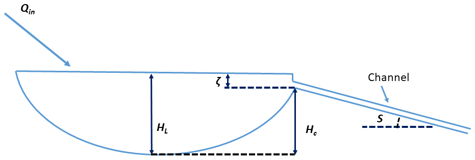
Figure 3 A schematic of the set-up for the slow-lake-drainage module. S is the slope of the channel's base, Q_in is the incoming discharge from its hydrological catchment, ζ represents the lake water that is about to overflow, H_c is the channel bed height above the lake bottom, and H_L is lake water depth.

The rate of change in the channel bed height above the lake bottom (H_C) is given as follows:

$$\begin{array}{}\text{(8)}& {\displaystyle \frac{\mathrm{d}{H}_{\mathrm{C}}}{\mathrm{d}t}}=-\mathit{\alpha }{\mathit{\zeta }}^{\mathrm{1.5}},\end{array}$$

where α is

$$\begin{array}{}\text{(9)}& \mathit{\alpha }={\displaystyle \frac{\mathit{\rho }{f}_{\mathrm{R}}}{\mathrm{8}L{\mathit{\rho }}_i}}{\left({\displaystyle \frac{\mathrm{2}g}{\mathrm{1}+\frac{f_{\mathrm{R}}}{\mathrm{4}S}}}\right)}^{\mathrm{1.5}}.\end{array}$$

Here, ρ is the density of water, assumed to be 1000 kg m⁻³; ρ_i is the density of ice, assumed to be 900 kg m⁻³; and L is the latent heat of the fusion of ice, assumed to be 334 kJ kg⁻¹.

For an overflowing SGL, the initial values of p, H_C, ζ, and S are determined from the lake geometry. Thereafter, in every time step, Eqs. (6)–(9) are solved for H_C and H_L. Following that, water volume lost by the SGL is estimated and is transferred to the destination as runoff via a meltwater channel downstream. In the following time step, this transferred runoff is available for further routing in the supraglacial-routing and lake-filling module. We then update the surface elevation of the DEM cells (i.e. those that lie along the supraglacial meltwater channel) that were eroded as a result of runoff transfer.

Therefore, through this mechanism, we are able to simulate the process of re-organization of supraglacial meltwater channels that occurs due to rapid lateral lake drainage (Karlstrom and Yang, 2016).

4.4 Lake-refreezing module

If an SGL undergoes no or only partial, drainage and if liquid meltwater remains in the lake at the onset of winter, observations show that this lake will then refreeze either fully or partially following the development of an ice lid. Our lake-refreezing model simulates the formation, growth, and subsequent decay of an ice lid based on the energy-balance-modelling concepts proposed by both Buzzard et al. (2017) and Law et al. (2020). The lake-refreezing model is one-dimensional and is applied to the deepest cell in each lake only (i.e. not all of the cells within a lake). As such, results represent a single point in x–y space, modelled as a 100 m,× 100 m column. We run the model at every time step, including when the near-surface air temperature is above zero and, as a result of which, the lake is unlikely to refreeze, in order to ensure that the column reaches the appropriate thermodynamic state for refreezing over winter. This model is divided into two stages, which are outlined below.

4.4.1 No lake ice

A lake is assumed to be capable of refreezing once any cell within the lake reaches 0.1 m in water depth. A vertical cross-section of the SGL at this stage is shown schematically in Fig. 4.

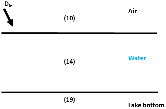
Figure 4 A schematic of the no-lake-ice stage of the lake-refreezing module. D_in represents the depth of meltwater contribution (in metres) to the lake from its corresponding hydrological catchment in every time step. Equations (10) and (19) are solved at the air–water and water–lake-bottom interfaces, respectively. Equation (14) is solved for the water in the lake. We assume that the lake bottom is an impermeable surface, i.e. ice or saturated firn or snow.

At the air–water interface, the heat budget equation is solved following Buzzard et al. (2017):

$$\begin{array}{}\text{(10)}& \begin{array}{rl}& (\mathrm{1}-I_{\mathrm{0}})\mathrm{SWR}(\mathrm{1}-\mathit{\alpha })+\mathit{\sigma }\left(T_{\mathrm{s}}^{\mathrm{4}}\right)+{\mathrm{LWR}}_{\mathrm{in}}\\ & +H+LE+F_{\mathrm{c}}\left(T_{\mathrm{s}}\right)=\mathrm{0}\end{array},\end{array}$$

where SWR is incoming shortwave radiation (W m⁻²) from MAR; I₀ represents the transmissivity of the lake, assumed to be 0.6 (e.g. Law et al., 2020; Buzzard et al., 2017); α represents the water surface albedo; and σ is the Stefan–Boltzmann constant, which is assumed to be $\mathrm{5.67}\times {\mathrm{10}}^{-\mathrm{8}}$ W m⁻² K⁻⁴. T_s is the lake surface temperature (K); LWR_in represents the incoming longwave radiation (W m²); H and LE are the sensible heat flux and latent heat flux, respectively (both in W m²); and F_c represents the heat flux due to convection in the lake (W m⁻²). Albedo (α) is formulated following Luthje et al. (2006):

$$\begin{array}{}\text{(11)}& \mathit{\alpha }={\displaystyle \frac{\mathrm{9702}+\mathrm{1000}{e}^{\mathrm{3.6}{h}_{\mathrm{lake}}}}{-\mathrm{539}+\mathrm{20}\mathrm{000}{e}^{\mathrm{3.6}{h}_{\mathrm{lake}}}}}.\end{array}$$

Here, h_lake represents the lake water depth (m). The LWR_in is the incoming longwave radiation, which we calculated following Banwell et al. (2012b):

$$\begin{array}{}\text{(12)}& \begin{array}{rl}& {\mathrm{LWR}}_{\mathrm{in}}=\\ & \left[\left(\mathrm{0.23}+\mathrm{0.484}{\left({\displaystyle \frac{e}{T_{\mathrm{a}}}}\right)}^{\frac{\mathrm{1}}{\mathrm{8}}}\right)\left(\mathrm{1}-n^{\mathrm{4}}\right)+\mathrm{0.952}{n}^{\mathrm{4}}\right]\mathit{\sigma }{T}_{\mathrm{a}}^{\mathrm{4}}\end{array},\end{array}$$

where n is the cloud cover, which ranges between 0 and 1; n=0 represents clear-sky conditions, and n=1 represents overcast conditions; e is the vapour pressure of the air (Pa); and T_a is the air temperature (K). The heat flux due to convection (F_c) is expressed according to the four-thirds rule:

$$\begin{array}{}\text{(13)}& F_{\mathrm{c}}\left(T_{\mathrm{s}}\right)=\mathrm{sgn}(T_{\mathrm{w}}-T_{\mathrm{s}})\left(\mathit{\rho }C\right)\mathrm{|}{T}_{\mathrm{w}}-T_{\mathrm{s}}{\mathrm{|}}^{\mathrm{4}/\mathrm{3}}.\end{array}$$

In the above equation, T_w represents the depth-averaged temperature of the water body (K), J is the turbulence heat flux factor and is assumed to be $\mathrm{1.907}\times {\mathrm{10}}^{-\mathrm{5}}$ m s⁻¹ K${}^{-\mathrm{1}/\mathrm{3}}$ (Buzzard et al., 2017), and C is the specific heat capacity of water and is assumed to be a constant (4186 J kg⁻¹ K⁻¹). T_w is expressed following Taylor and Feltham (2004):

$$\begin{array}{}\text{(14)}& (\mathit{\rho }c{)}_{\mathrm{l}}{h}_{\mathrm{w}}{\displaystyle \frac{\partial T_{\mathrm{w}}}{\partial t}}=-F_{\mathrm{c}}\left(T_{\mathrm{l}}\right)-F_{\mathrm{c}}\left(T_{\mathrm{s}}\right)-\mathrm{FSW},\end{array}$$

where (ρc)_l is the volumetric heat capacity of the lake water body (JK⁻¹ m⁻³), h_w is the height of the water in the lake (m), and FSW is the total solar radiation that penetrates through the lake surface (Jm⁻² s⁻¹) (see Appendix D). F_c(T_l) is the convective heat flux at the lake bottom and is expressed by Eq. (13), and T_l is the temperature at that boundary, assumed to be 273.16 K. This equation is solved in the lake.

H and LE are sensible heat flux and latent heat flux, respectively, and are expressed as follows:

$$\begin{array}{}\text{(15)}& {\displaystyle }H={\mathit{\rho }}_{\mathrm{a}}{C}_{p_{\mathrm{air}}}{C}_{T}u(T_{\mathrm{a}}-T_{\mathrm{s}}),\text{(16)}& {\displaystyle }LE={\mathit{\rho }}_{\mathrm{a}}L{C}_{T}u(q_{\mathrm{a}}-q_{\mathrm{s}}),\end{array}$$

where ρ_a is the density of air (kg m⁻³); $C_{p_{\mathrm{air}}}$ is the specific heat capacity of air at constant pressure; u is the air speed (m s⁻¹); L is the latent heat of vaporization of the water, assumed to be 2.5×10⁶ J Kg⁻¹; and q_a and q_s represent the specific humidity of the air and water surface, respectively. C_T is a function of atmospheric stability following Ebert and Curry (1993):

$$\begin{array}{}\text{(17)}& \begin{array}{rl}& C_T=C_{T_{\mathrm{0}}}\left(\mathrm{1}-{\displaystyle \frac{\mathrm{2}b{R}_i}{\mathrm{1}+c{\left|R_i\right|}^{\frac{\mathrm{1}}{\mathrm{2}}}}}\right),R_i<\mathrm{0}\\ & C_T=C_{T_{\mathrm{0}}}(\mathrm{1}+b{R}_i{)}^{-\mathrm{2}},R_i\ge \mathrm{0}\end{array}.\end{array}$$

Here, $C_{T_{\mathrm{0}}}=\mathrm{0.0013}$, b=20, and c=50.986 are constants. R_i is the bulk Richardson number and is expressed as follows:

$$\begin{array}{}\text{(18)}& R_i=g{\displaystyle \frac{(T_{\mathrm{a}}-T_{\mathrm{s}})}{T_{\mathrm{a}}{v}^{\mathrm{2}}}}\mathrm{\Delta }z,\end{array}$$

where Δz is the thickness of the layer of the atmosphere between two constant pressure surfaces (Ebert and Curry, 1993) equal to 10 m.

The elevation of the lake bottom can either move up due to basal freeze on or move down due to enhanced lake bottom ablation. The movement of the elevation of the lake bottom elevation is described following Buzzard et al. (2017):

$$\begin{array}{}\text{(19)}& \mathit{\rho }L{\displaystyle \frac{\partial h_{\mathrm{l}}}{\partial t}}=k{\displaystyle \frac{\partial T}{\partial z}}+F_{\mathrm{c}}\left(T_{\mathrm{l}}\right)\end{array}$$

where h_l is the elevation of the lake bottom; k is the conductivity of ice; and L is the latent heat of the fusion, assumed to be a constant equal to 334 kJ kg⁻¹. In practice, we find that the movement of the lake bottom is 2 orders of magnitude smaller than the movement of the lake surface as a result of meltwater accumulation. This equation is solved at the lake bottom.

4.4.2 Lake ice

When the energy balance at the lake surface becomes negative, the lake starts to refreeze, and a layer of ice forms on the surface. Following Buzzard et al. (2017), the amount of refreezing is calculated over consecutive time steps, and the total for the grid cell is recorded. This process is continued until a stable ice lid forms over the lake, defined as occurring when the total ice thickness of a grid cell equals or exceeds 0.1 m. Once such an ice lid is formed, the refreezing module switches from the no-lake-ice stage to the lake ice stage. A schematic for the lake ice stage is shown in Fig. 5.

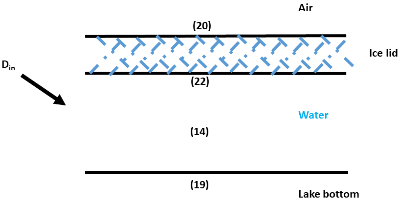
Figure 5 A schematic of the lake ice stage of the lake-refreezing module. D_in represents the depth of the meltwater contribution (in metres) to the lake from its hydrological catchment in every time step. Equations (20) and (19) are solved at the air–ice-lid and water–lake-bottom interfaces, respectively. Equation (22) estimates the movement of the lid–lake interface in every time step. Equation (14) is solved for the lake water.

The energy balance at the air–ice-lid interface (Q_ice) is given by the following:

$$\begin{array}{}\text{(20)}& Q_{\mathrm{ice}}=\mathrm{SWR}(\mathrm{1}-{\mathit{\alpha }}_{\mathrm{s}})+\mathit{\sigma }\left(T_{\mathrm{s}}^{\mathrm{4}}\right)+{\mathrm{LWR}}_{\mathrm{in}}+H+LE+G.\end{array}$$

Here, α_s is the surface albedo of the lake ice and is assumed to be a constant equal to 0.431 (Buzzard et al., 2017); T_s is the surface temperature of the ice lid (K); and H and LE are modelled from Eqs. (15) and (16), respectively. G (W m⁻²) is conductive heat flux flowing from the ice lid's surface to the lake water underneath it and is calculated as follows:

$$\begin{array}{}\text{(21)}& G=k{\displaystyle \frac{T_{\mathrm{s}}-T_{\mathrm{sl}}}{\mathrm{\Delta }{z}_i}},\end{array}$$

where k is the thermal conductivity of ice, assumed to be a constant equal to 2.24 W m⁻¹ K⁻¹, and T_sl is the temperature at the base of the ice lid which is in contact with the lake water. The value of T_sl is assumed to be at the melting point, i.e. 273.16 K, and Δz_i is the thickness of the ice lid (m). The lake-refreezing model is run at daily time steps, and so the temperature profile within the ice lid is assumed to be linear over time periods of days and weeks (e.g. Nicholson and Benn, 2006).

Once a stable ice lid forms, the surface temperature of the lid is estimated at every time step by solving Eq. (20). Melting on the ice lid's surface occurs whenever the energy balance becomes positive. For simplicity, in every time step, both the meltwater produced on the lid's surface and the meltwater contributed by the lake's hydrological catchment is pushed underneath the ice lid. Further, any change in the heat content of the lake water due to the addition of meltwater from the lid and the lake catchment is neglected (Law et al., 2020).

The movement of the ice-lid–lake boundary is described by a Stefan equation (e.g. Buzzard et al., 2017) and is expressed as follows:

$$\begin{array}{}\text{(22)}& \mathit{\rho }L{\displaystyle \frac{\partial h_u}{\partial t}}=k{\displaystyle \frac{\partial T}{\partial z}}+F_{\mathrm{c}}\left(T_u\right).\end{array}$$

Here, T_u is the temperature of the ice lid's base and is assumed to be a constant equal to 273.16 K. h_u is the elevation of the lid–lake boundary (m).

5 Results

5.1 Model calibration

We first ran a sequence of calibration steps in order to fix the values for three key parameters used in the model: (i) critical stress threshold of ice (τ_c – used in the hydrofracture module), (ii) crevasse width (w_c – used in the hydrofracture module), and (iii) supraglacial meltwater channel width (w – used in the slow-lake-drainage module).

Previous studies have shown that, over a given region on the ice sheet, the value of τ_c determines the spatial distribution and density of the crevasses (e.g. Clason et al., 2012, 2015). Crevasses are more abundant with lower values of τ_c because it is more likely that surface stress exceeds this value. The value of w_c determines the spatial distribution and density of moulins (e.g. Clason et al., 2012, 2015). A crevasse with a narrower width requires less meltwater input to produce a greater water depth, and therefore, vertical crevasse propagation (i.e. hydrofracture) can occur more readily, resulting in moulin formation (e.g. Clason et al., 2012; Banwell et al., 2016). Keeping this in mind, we calibrated τ_c and w_c simultaneously by comparing (a) daily annual observed (from MODIS) and modelled lake areas and (b) daily annual observed and measured proglacial discharge.

We ran our model using a range of values for τ_c and w_c (Fig. 6a, b); for τ_c, we used a range of von Mises values between 200–300 kPa (200, 240, 260, 280, and 300 kPa) following Hoffman et al. (2018), Koziol et al. (2017), and Clason et al. (2012, 2015), and for w_c, we used a range of values between 0.01–2 m (0.05, 0.2, 0.5, 0.6, 1, and 2 m) after Krawczinsky et al. (2009) and Clason et al. (2012, 2015). Since region 1 is heavily crevassed and has few SGLs, which are mostly very small (∼ < 0.02 km²), and since stress data are not available for region 3, the calibration procedure for τ_c and w_c was done for region 2 only for the year 2019. We found that using τ_c and w_c of 280 kPa and 0.6 m, respectively, gave the best agreement with observations. The root mean squared error (RMSE) between modelled and observed daily lake area was 9.7 km², and the modelled maximum daily lake area (38 km²) was in good agreement with that which was observed (40 km²). The RMSE between modelled and observed daily proglacial discharge was 1.46×10⁷ m³, and modelled annual proglacial discharge (4.3×10⁹ m³) was also in good agreement with that which was observed (4.1×10⁹ m³). These values of τ_c and w_c were used for all subsequent model simulations. We note that we see a lag between the start of proglacial discharge in the model and in the observations; this is apparent with all combinations and can be attributed to the fact that our model does not include subglacial hydrology and to the time it takes for the water to pass through the subglacial system. We see significantly larger daily lake areas in the latter part of the melt season in the model; this can be attributed in part to (a) uncertainty in our model (there is much more meltwater available in these months, which may amplify process-based uncertainty) and (b) uncertainty in the observations (we see more missing data due to cloud cover later on in the year).

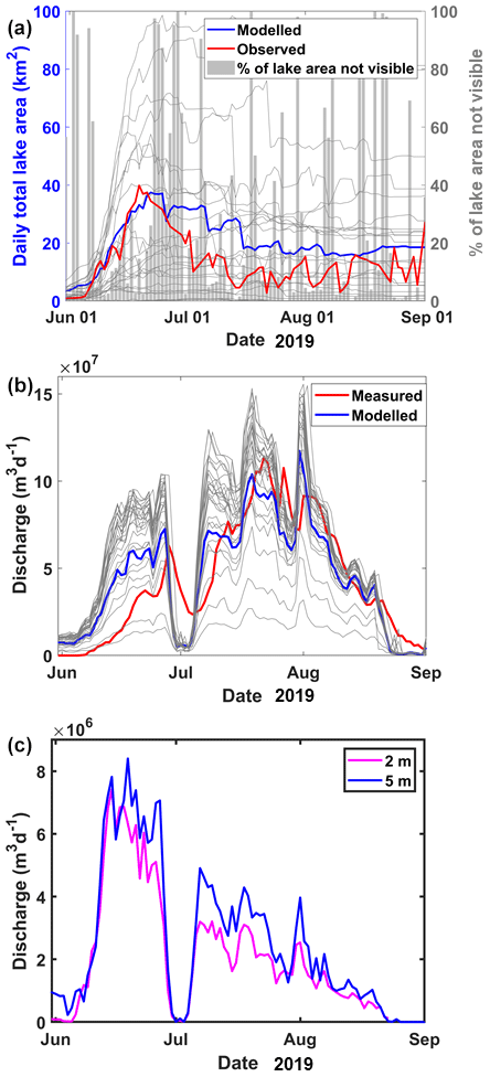
Figure 6 (a) Comparison of the modelled and observed daily total SGL areas for different pairs of τ_c and w_c for region 2 in 2019. The observed curve is shown in red, and the modelled curve for the optimum pair of τ_c and w_c (i.e. for τ_c=280 kPa and w_c=0.6 m) is shown in blue. The modelled curves for other combinations of τ_c and w_c are shown in grey. The right y axis represents the daily average percentage of total SGL area that is not visible in the MODIS imagery; only those days where the daily total visible lake area was more than 80 % are plotted on the red line. (b) Comparison of modelled and measured daily total meltwater discharge for different pairs of τ_c and w_c for region 2 in 2019. The observed curve is shown in red, and the modelled curve for the optimum pair of τ_c and w_c (i.e. for τ_c=280 kPa and w_c=0.6 m) is shown in blue. The modelled curves for other combinations of τ_c and w_c are shown in grey. (c) Sensitivity of channel-incision-based lake overflow discharge for two values of channel widths (i.e. 2 and 5 m) for region 2 in 2019.

Third, we assessed the sensitivity of the daily modelled proglacial discharge to the width of supraglacial meltwater channels (w) originating at the outlet of overflowing SGLs. To do this, we simulated the process of slow lake drainage for a range of channel width scenarios between 2 m (Kingslake et al., 2015) and 5 m (Koziol et al., 2017) for 2019 for region 2 (Fig. 6c). We find that the total modelled drainage is relatively insensitive to the choice of channel widths, though in line with Kingslake et al. (2015), a narrower channel width leads to slightly lower total discharge over the melt season: 1.9×10⁸ and 2.3×10⁸ m³ d⁻¹ for a 2 and 5 m wide channel, respectively (Fig. 6c). For our model simulations, we use 5 m as the channel width.

We also considered the effect of fracture toughness (K_IC) and the roughness coefficient of stream beds (f_R) on modelled discharge, but we found that the modelled discharge was insensitive to the values of these parameters.

5.2 Water-routing and lake-filling module

Using the parameter values constrained in Sect. 5.1, we then evaluated the performance of the water-routing and lake-filling component of our model by comparing all the modelled lake extents (i.e. with no filtering applied) with those observed from satellite imagery during the melt season of 2019 for region 2, which has an abundant population of lakes and sufficient forcing data to model hydrofracture and rapid lake drainage (Fig. 7). Our model performed well in terms of predicting observed lake locations; 80 % of the observed lake locations coincided with modelled lakes. Some SGLs were observed but not modelled; this is likely because the DEM used by the model does not have depressions at those locations, presumably because the DEM was created using satellite imagery from winter or early spring, when many of the depressions would have been filled with snow or refrozen lake water from the melt season prior to acquisition. Some SGLs were modelled but not observed; this can be attributed mainly to size – lakes smaller than 13 DEM pixels are not resolved by MODIS, and ∼ 71 % of our modelled lakes were smaller than this size. Other sources of uncertainty include cloud cover in the observations, filtering in the observations (shapes that appear less than twice in 6 d are removed; this could result in the removal of short-lived lakes from the dataset), and uncertainty in the spatial distribution of MAR-predicted runoff.

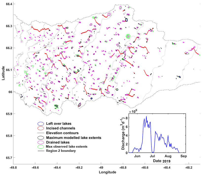
Figure 7 Map of supraglacial lakes in region 2 in 2019. Maximum extents of modelled lakes that contain water at the end of the melt season are shown in black. Maximum extents of modelled lakes that have drained are shown in magenta. Supraglacial channels created by lake overflow and drainage are shown in red. Maximum observed lake extent is shown in green. Surface elevation contours are labelled in grey. Inset: total discharge of surface meltwater from the SGLs that drain via overflow (i.e. those with red paths leading from them in (a)) in region 2 for the 2019 melt season.

Our model was able to simulate the formation of 808 lakes in region 2. Out of these lakes, 463 (57.3 %) lakes drained either fully or partially but exclusively via hydrofracture, 256 (31.6 %) lakes drained either fully or partially but exclusively via overtopping, 48 (5.9 %) lakes initially drained via overtopping but later drained via hydrofracture, 261 (32.3 %) lakes partially drained and then refroze, and 92 (11.4 %) lakes did not drain at all and then later refroze. This suggests that some lakes exhibit more complex behaviour than suggested in the literature, where lakes are typically partitioned between three independent modes: fast draining, slow draining, and refreezing (Selmes et al., 2013; Fitzpatrick et al., 2014; Miles et al., 2017; Williamson et al., 2017, 2018a, b). We note that the modelled daily average flow velocity of the meltwater runoff transfer between a DEM cell and its corresponding destination cell was in the range of 0.001–0.462 m s⁻¹. This is in line with that observed by Smith et al. (2015) and Yang et al. (2018), which is 0.2–9.4 m s⁻¹.

5.3 Slow-lake-drainage module

In order to model the distribution of water transiently stored in SGLs, we first need to be able to model the transfer of water out of lakes via lateral drainage across the ice sheet. This typically occurs by overtopping and channel incision and is a slower mode of drainage than hydrofracture.

All supraglacial meltwater pathways modelled for region 2 at the end of the 2019 melt season are shown in Fig. 7. Our analyses show that the meltwaters overflowing from the SGLs in this region were able to incise meltwater channels to depths up to ∼ 2 m; this is in good agreement with other studies that predict channel depths of ∼ 1 m for stably draining lakes (i.e. those where the rate of lake-level drawdown exceeds the rate of channel incision; Kingslake et al., 2015) and about 5 m for unstably draining lakes (which always drain completely; e.g. Koziol et al., 2017). The meltwater channels flowing out of SGLs first start to form at lower elevations, i.e. where SGLs drain earlier in the season, and then spread inland as the melt season progresses, following the progression of the lakes to higher elevations on the ice sheet.

Our analyses show that, in just a single day, these supraglacial meltwater channels have the capability to transfer meltwater over distances varying between a few hundreds of metres to tens of kilometres, between one SGL and another, or between an SGL and a crevasse or to drain off the ice sheet into the proglacial area. Figure 6c shows the total modelled daily volume of meltwater that drained via surface overflow from SGLs via meltwater channels for the melt season of 2019. The maximum volume of modelled daily discharge was ∼ 8.0×10⁶ m³, and this occurred in mid-June 2019. In total, the modelled discharge was ∼ 1.2×10⁸ m³ during the month of June. From mid-July until the end of August, an overall decrease in the daily modelled discharge was observed due to the decrease in meltwater production.

Figure 8a and b show the evolution of the water depth and volume of an SGL located in region 2 (refer to Fig. 1 for location), as well as the meltwater channel depth leading out of the SGL. This lake was chosen because it was present in the observed set of lakes and because it underwent partial drainage via overtopping. In our simulation, the lake level exceeded the channel height on 14 June 2019, and after this, overflowing lake water progressively melted the base of the supraglacial channel, incising it downwards until 20 June 2019. On 20 June 2019, the lake drained rapidly via hydrofracture as a result of a large influx of meltwater.

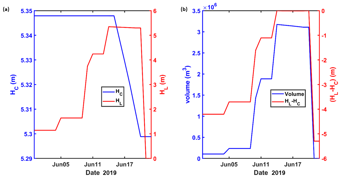
Figure 8 (a) Evolution of lake water depth (H_l, red line) and height of the meltwater channel bed above the lake bottom (H_c, blue line); (b) evolution of lake water volume (blue line) and difference in lake and channel height (red) for the SGL denoted by the green circle in Fig. 1 during June 2019. For more clarity on the variables plotted, please refer to slow-lake-drainage Module schematic in Fig. 3.

5.4 Hydrofracture and lake drainage module

We model hydrofracture through crevasses that form outside of lakes and also through crevasses that form beneath lakes. Both of these provide a mechanism to transfer water from the surface of the ice sheet to the base, where it is routed to the ice sheet margin and expelled out from under the ice sheet as proglacial discharge. In order to evaluate the performance of the hydrofracture and lake drainage module in our model, we compare modelled proglacial discharge to that observed in region 1 between 2015 and 2019 (inclusive) and in region 2 in 2019 (Fig. 9, Table 2).

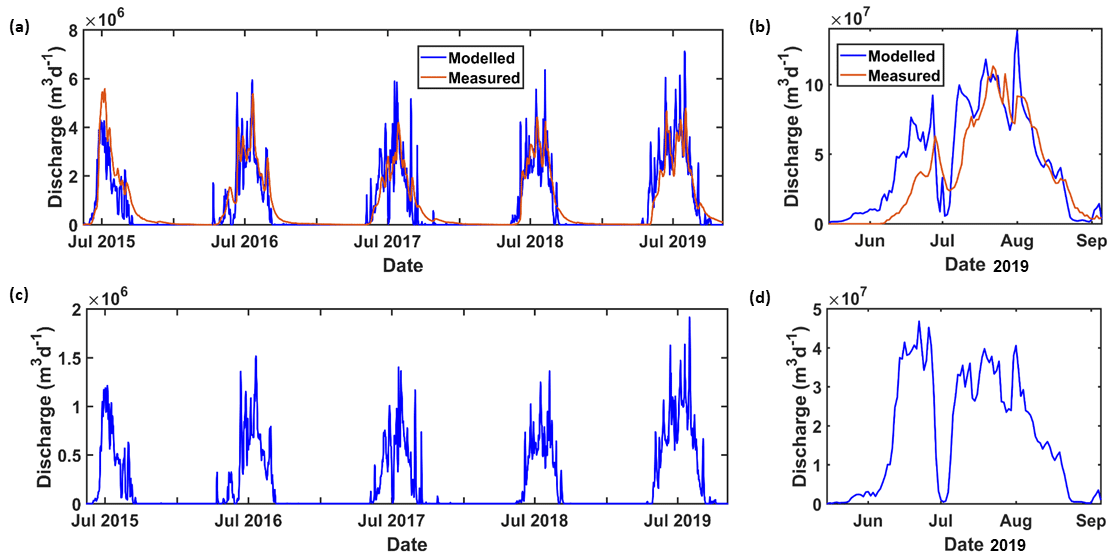
Figure 9 (a) Modelled and measured proglacial discharge for region 1 from 2015 to 2019. (b) Modelled and measured proglacial discharge for region 2 for just 2019. (c) Daily modelled discharge due to rapidly draining SGLs and the corresponding moulins (after the SGL has drained) in region 1 for all melt seasons from 2015 to 2019. (d) Daily modelled discharge from rapidly draining SGLs and the corresponding moulins (after the SGL has drained) in region 2 for just 2019. For all plots, tick marks on the x axis are on the first day of each month. Please also note that each plot has a different scale on the y axis.

Table 2 Comparison between modelled and observed total annual proglacial discharge for regions 1 (2015 to 2019) and 2 (2019 only). Modelled density of lake bottom moulins also shown.

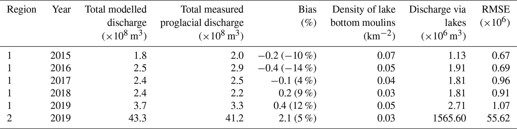
In region 1, for all years, the total annual modelled proglacial discharge matched well with that observed (Table 2), deviating by a maximum of 14 %, a minimum of 4 %, and 10 % on average. In region 2, the difference was higher at 17 %. For region 1, this is within the uncertainty of the MAR data, which is ±15 % (Fettweis et al., 2020). Modelled inter-annual variability in total annual proglacial discharge in region 1 was also in very good agreement with observations (r=0.9).

In region 1, the date for which our model simulates water beginning to drain away from the surface through both draining lakes and non-lake crevasses varies by about 1 month. The earliest we see this occur in our data is in 2016, where it begins on the 11 April. The latest we see this occur is in 2015, were it begins on the 18 May 2015. For region 1, the observed proglacial discharge begins around about the same time as that predicted by our model but with a lag of ∼ 2–3 d, likely due to the fact that our supraglacial hydrology model is not coupled to a subglacial routing model and hence does not simulate the time taken for water to flow through the subglacial environment to the ice sheet margin. This is in good agreement with other modelling studies conducted in the Paakitsoq region of Greenland that have shown a delay of 2 to 3 d (e.g. Banwell et al., 2013, 2016). Proglacial discharge generally ceases in September in both the observations and model in both regions. Seasonal and sub-seasonal temporal variability in proglacial discharge is captured well by our model in both region 1 (r=0.96 on average) and region 2 (r=0.88 for 2019).

Temporal variability in proglacial discharge is driven by temporal variability in the MAR runoff; for example, in region 1 and in region 2, the maximum daily modelled proglacial discharge occurs on 1 August 2019 (7.1×10⁶ m³), which is the same day that MAR simulates its highest daily total runoff since 1950 (Fig. A1). For region 2 in 2019, runoff in MAR begins around 1 month before observed proglacial discharge. As a result, our modelled proglacial discharge lags behind that observed around the same time. This is likely a result of the uncertainty in the MAR projections; for instance, we note that MAR runoff occurs about 1 week earlier than proglacial discharge in region 1 in 2019 as well.

We also examined the sensitivity of total annual discharge to MAR runoff. For this, we carried out an experiment for region 2 where we ran the model by varying the runoff by ±15 %. We found out that the total annual discharge decreased by 13 % when the daily MAR runoff was reduced by 15 %. When the MAR runoff was increased by 15 %, the total annual discharge increased by 25 %, likely due to an increase in the formation of moulins in our simulation.

Differences between model performance in region 1 and region 2 are likely due to the processes controlling the transfer of water from the surface to the bed in each region. In region 1, proglacial discharge is dominated by the hydrofracture of crevasses that are not within SGLs. In this region, we predict that 86 % of MAR runoff drained to the bed, of which 0.5 % was drained through lakes and 99.5 % through non-lake crevasses, respectively. Region 2 has many more lakes, and so the contribution of draining lakes to proglacial discharge is much larger; for region 2, we predict that 71 % of MAR runoff drained to the bed, of which 38 % and 62 % were drained through lakes and non-lake crevasses, respectively, which is in keeping with findings from other studies (Koziol et al., 2017). Our simulations also showed that the meltwater that runs over the surface only towards and off of the edge of the ice margins is at least 2 orders of magnitude less than that which passes through the englacial and subglacial environments enroute.

If we assumed that all surface-to-bed connections formed due to the rapid drainage of SGLs become moulins, our modelled moulin density ranged between 0.03–0.07 moulins km⁻² in region 1 from 2015 to 2019 and was 0.08 moulins km⁻² for region 2 in 2019. These values of lake bottom moulin density are in agreement with those observed by Colgan and Steffen (2009; 0–0.88 km⁻²), Banwell et al. (2016; 0–0.2 km⁻²), and Zwally et al. (2002; 0.2 km⁻²). We note that both draining lakes and non-lake crevasses deliver water to the bed, initially near the ice sheet margin, where the ice is thin compared to higher elevations, and that this spreads inland as the melt season progresses, which is also in line with the findings of previous studies (e.g. Fitzpatrick et al., 2014; Christoffersen et al., 2018).

5.5 Lake-refreezing module

In order to model the full life cycle of supraglacial lakes – and to quantify the amount of water already stored on the ice sheet before the onset of the melt season – it is important to capture the freezing process at the end of the melt season and the unfreezing process at the beginning.

Satellite observations show that no lakes in region 1 or region 2 refreeze at the end of the melt season, and so we use a case study lake located in region 3 to evaluate our lake-refreezing model (Fig. 1). The case study lake is ∼ 0.6 km² in area and has a perimeter of ∼ 3.2 km according to Google Earth imagery (Fig. 10c). This is a relatively large lake compared to others in southwest Greenland (Banwell et al., 2014).

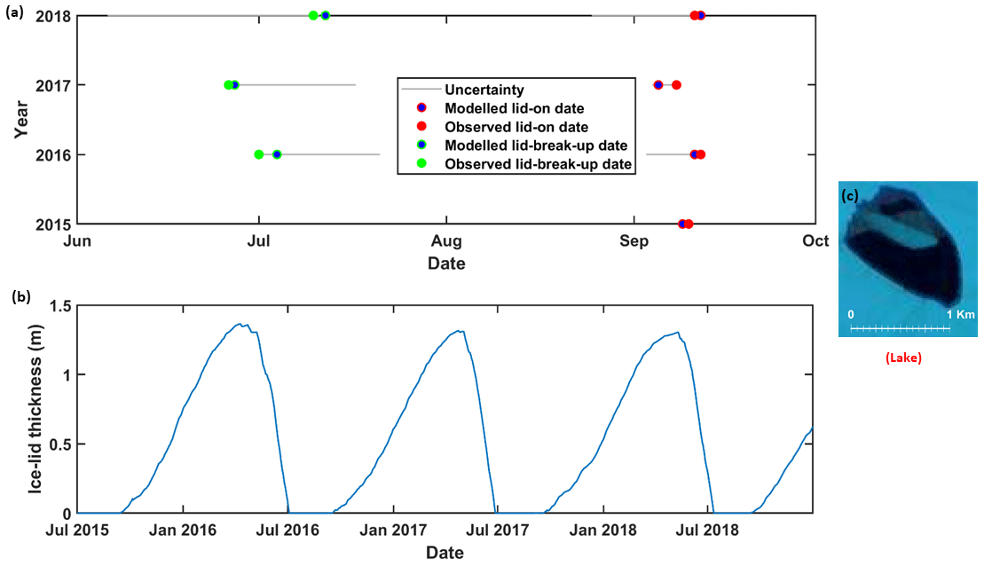
Figure 10 (a) Comparison of modelled lid-on and lid-break-up dates with those observed from Sentinel-2 satellite imagery for a lake in region 3 (see Fig. 1a for location). Error bars (grey lines) for observed break-up data are the time between two images where the lake is less than 30 % open water and then greater than or equal to 30 % open water (at the start of the melt season) or greater than 30 % open water and then not visible (at the end of the melt season). (b) Evolution of lake ice lid thickness over the course of three freezing–melt seasons from 2015 to 2018. (c) Dimensions of the lake (post lid break-up) as seen from Sentinel-2 imagery. Though part of the ice lid is still present, since more than 30 % of the lake area is clearly visible, we consider the lake to be ice lid free.

The evolution of this lake was modelled from 1 July 2015 until December 2018 over three complete freezing–melt cycles (Fig. 10). From 2016 to 2018, this SGL was observed in Sentinel-2 satellite imagery to persist throughout each of the three melt seasons and then to develop an ice lid over each of the following winters. For the observations, we define the lid-on date as the date when the SGL forms an ice lid across its entire water surface; for the model, we define the lid-on date as the date when the ice lid on top of a lake exceeds 0 m . The observed lid-break-up date is defined as the date (i.e. the first sighting from the satellite imagery) when around 30 % of the SGL water surface becomes exposed (e.g. Duguway et al., 2003). The modelled lid-break-up date is defined as the day when the ice lid thickness becomes zero (e.g. Law et al., 2020).

Modelled and observed lid-on dates are in good agreement; modelled lid-break-up dates occur slightly later (∼ 2 d) than observed dates in all 3 years (Fig. 10). In all years, the modelled and observed SGL lid-on dates fall in early September, and lid-break-up dates fall in late June or in early July. Our model analyses showed that, for all years, the SGL ice lid thickness reached a maximum in early April, and the thickest modelled ice lid was ∼ 1.4 m in the year 2016. This is within the range of values suggested in previous modelling and field studies (e.g. Koenig et al., 2015; Law et al., 2020). The lake did not refreeze entirely; in each year, there was at least 1 m of liquid-water depth beneath the lake. This is reasonable since previous studies have shown that lakes with depths of more than ∼ 1.3 m can persist as liquid water through the winter once an ice lid has formed (Law et al., 2020).

6 Conclusions

We present a new supraglacial hydrology model for the Greenland Ice Sheet and show that it is able to simulate lake formation and growth, lake drainage, lake refreezing, and the drainage of water from the surface to the bed through crevasses outside of lakes in southwest Greenland. We are able to simulate 80 % of observed lake locations, produce lake bottom moulin density estimates that are consistent with previous work, and simulate the temporal evolution of both daily lake area and proglacial discharge with reasonable fidelity (RMSE = 9.7 km² and 1.46×10⁷ m³). This gives us confidence in the ability of our model to determine where, when, and how much water gets to the base of the ice sheet.

Observational studies typically assume three independent modes of lake cessation, rapid vertical drainage, slow lateral drainage, or refreezing (e.g. Selmes et al., 2012). Our modelling work suggests that, in actuality, some (∼ 6 %) lakes exhibit more complex behaviour than this and can drain via a combination of both slow lateral drainage and rapid hydrofracture-driven drainage. Similarly, we model a significant number of lakes that drain partially via slow lateral drainage, with the remaining water subsequently refreezing.

We note that our model is sensitive to uncertainty in forcing data, including estimates of runoff produced by MAR, which control the timing and rate of meltwater flux through the system, and the DEM used to route and pond meltwater, which controls where lakes form and limits their maximum size. We also note that the application of our model is limited by the availability of forcing data, especially monthly ice velocities.

We find – in agreement with previous work – that the bulk of hydrofracture-related drainage events (62.0 %–99.5 %) occur via crevasses that were not part of an SGL, but this is spatially variable, with the balance shifting further towards drainage through SGLs in large basins that extend far inland. We also see temporal variability in this signal, with the proportion of water draining through lakes being higher in the early part of the melt season, presumably before the development of an extensive moulin network as a result of draining lakes.

To the best of our knowledge, this is the most complete model of supraglacial hydrology on the GrIS to date. The next step is therefore to use our model predictions of basal-water injection to drive a subglacial model and ultimately to examine the impact of seasonal meltwater supply variability on ice sheet flow. Ultimately, our intention is to couple our model with a model of both ice flow and subglacial hydrology. This will allow us to update the DEM's surface elevation due to ice flux and surface melting, which will enable us to simulate other observed processes such as rapid SGL drainage owing to transient changes in the ice velocities (e.g. Christofferson et al., 2018) and the re-organization of supraglacial meltwater channels as a result of rapid vertical drainage events (e.g. Karlstrom and Yang, 2016).

Appendix A: Tables and figures

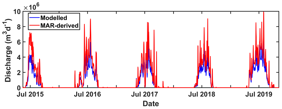
Figure A1 Comparison between daily discharge modelled by MAR (red) and modelled in our study (blue) for region 1 for the years 2015, 2016, 2017, 2018, and 2019.

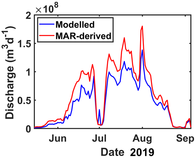
Figure A2 Comparison between daily discharge modelled by MAR (red) and modelled in our study (blue) for region 2 for 2019.

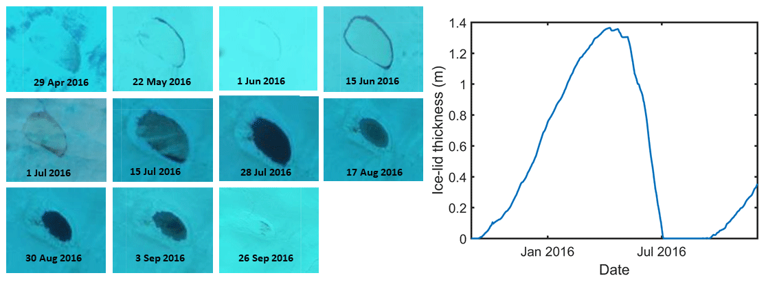
Figure A3 Sentinel-2 imagery observed and modelled evolution of ice lid thickness for the lake located in region 3 (for location, see the black triangle in Fig. 1).

Table A1 List of satellite imagery used to determine lid-on and lid-break-up dates.

Appendix B: Estimation of potential destination cell (PDC), the corresponding flow path, and lake-filling algorithm in the supraglacial-routing and lake-filling module

B1 Estimation of PDC and the corresponding flow path

We first define a three-by-three neighbourhood around a DEM cell (i.e. origin). The neighbourhood DEM cell with the lowest surface elevation is chosen as the next cell to which all the meltwater runoff from the origin will flow uniformly. If this cell is neither a sink (i.e. surface depression) nor a crevasse, the above procedure is repeated till a sink or a crevassed cell is located, which finally becomes the PDC of the origin. All the DEM cells through which the meltwater runoff flows enroute from the origin to the PDC constitute the flow path. In the case where the origin cell is a sink or a crevasse, the meltwater runoff stays put as the origin cell becomes its own PDC, and the length of the flow path traversed by the meltwater runoff is zero.

B2 Lake-filling algorithm

In every time step and for every sink cell where meltwater runoff has accumulated, we delineate the hydrological catchment that feeds the sink cell. This is done by locating all the DEM cells that have the sink cell as their PDC. We then locate the catchment outlet which is generally the lowest-lying catchment boundary cell (e.g. Arnold, 2010). The maximum lake extent and the corresponding volume are estimated from the elevation of the outlet cell. The accumulated meltwater runoff is then used to fill up the depression's catchment till the modelled SGL's water surface elevation becomes equal to that of the catchment's outlet cell. The excess meltwater runoff will overflow in the form of supraglacial meltwater water channels in the overtopping and drainage module (i.e. in module 3).

Appendix C: Derivation of equations of evolution of lake depth and channel depth in the overtopping and drainage module

The lake volume and the lake depth of an SGL can be related as follows (Kingslake et al., 2015):

$$\begin{array}{}\text{(C1)}& {\left({\displaystyle \frac{H_{\mathrm{L}}}{H_{\mathrm{Li}}}}\right)}^{p_{\mathrm{L}}}={\displaystyle \frac{V_{\mathrm{L}}}{V_{\mathrm{Li}}}},\end{array}$$

where H_L and V_L represent the lake depth and lake volume at any given time step, respectively. H_Li and V_Li represent the lake depth and lake volume prior to any event of channelized drainage, respectively. p_L is a constant and is defined as follows:

$$\begin{array}{}\text{(C2)}& A_{\mathrm{Li}}={\displaystyle \frac{p_{\mathrm{L}}{V}_{\mathrm{Li}}}{H_{\mathrm{Li}}}}.\end{array}$$

For our analyses, the value of p_L is assumed to be 1.5. This value was determined by Kingslake et al. (2015) after analysing the hypsometry of an SGL that was monitored by Georgiou et al. (2009).

With a meltwater input of Q_in and meltwater discharge at the lake's outlet, i.e. Q, the lake depth evolution can be expressed as follows:

$$\begin{array}{}\text{(C3)}& {\displaystyle \frac{\mathrm{d}{H}_{\mathrm{L}}}{\mathrm{d}t}}={\displaystyle \frac{\mathrm{1}}{A_{\mathrm{Li}}}}{\left({\displaystyle \frac{H_{\mathrm{Li}}}{H_{\mathrm{L}}}}\right)}^{p_{\mathrm{L}}-\mathrm{1}}\left(Q_{\mathrm{in}}-Q\right).\end{array}$$

On applying Bernoulli's equation at the lake centre and at the lake outlet (Fig. 3),

$$\begin{array}{}\text{(C4)}& H_{\mathrm{L}}=\left(H_{\mathrm{C}}+D\right)+{\displaystyle \frac{v^{\mathrm{2}}}{\mathrm{2}g}},\end{array}$$

where D is the depth of flow, and v is the velocity of meltwater in the in the supraglacial channel. Along the channel's length, the shear stress (τ_F) exerted on the water by the ice can be formulated with the Darcy–Weisbach equation:

$$\begin{array}{}\text{(C5)}& {\mathit{\tau }}_F={\displaystyle \frac{\mathrm{1}}{\mathrm{8}}}{f}_{\mathrm{R}}{\mathit{\rho }}_{\mathrm{w}}{v}^{\mathrm{2}},\end{array}$$

where f_R is the channel's hydraulic roughness, and ρ_w is the density of water (1000 kg m⁻³). The ice mass (m) melted per unit length of the channel per unit time is

$$\begin{array}{}\text{(C6)}& m={\displaystyle \frac{{\mathit{\tau }}_{F}vw}{L}},\end{array}$$

where L is the latent heat of the fusion of ice (334 kJ kg⁻¹), and w is the channel width that is assumed to be a constant throughout the channel. From Eqs. (8) and (11), the rate of change of the height of the channel bottom above the lake bed, i.e. H_C, can be expressed as follows:

$$\begin{array}{}\text{(C7)}& {\displaystyle \frac{\mathrm{d}{H}_{\mathrm{C}}}{\mathrm{d}t}}=-{\displaystyle \frac{f_{\mathrm{R}}{\mathit{\rho }}_{\mathrm{w}}}{\mathrm{8}L{\mathit{\rho }}_{\mathrm{i}}}}{v}^{\mathrm{3}},\end{array}$$

where ρ_i is density of ice (900 kg m⁻³). The along-channel gravitational driving stress (τ_G) is

$$\begin{array}{}\text{(C8)}& {\mathit{\tau }}_{\mathrm{G}}={\mathit{\rho }}_{\mathrm{w}}gDS,\end{array}$$

where S is the supraglacial channel's bed slope. Assuming steady meltwater flow in the channel, we do a force balance by equating Eqs. (A5) and (A8) and consequently arrive at an expression for water discharge at the lake's outlet, i.e. Q:

$$\begin{array}{}\text{(C9)}& Q=\sqrt{{\displaystyle \frac{\mathrm{8}gS}{f_{\mathrm{R}}}}}w{D}^{\frac{\mathrm{3}}{\mathrm{2}}}.\end{array}$$

The lake outflow at the outlet (i.e. Q) can be expressed in terms of water velocity (v), water depth in the channel (D), and channel width (w) as follows:

$$\begin{array}{}\text{(C10)}& Q=vwD.\end{array}$$

Eliminating D and v from Eqs. (A4), (A9), and (A10), the final expression for H_C is

$$\begin{array}{}\text{(C11)}& {\displaystyle \frac{\mathrm{d}{H}_{\mathrm{C}}}{\mathrm{d}t}}=-{\displaystyle \frac{f_{\mathrm{R}}{\mathit{\rho }}_{\mathrm{w}}}{\mathrm{8}L{\mathit{\rho }}_{\mathrm{i}}}}{\left({\displaystyle \frac{\mathrm{2}g}{\mathrm{1}+\frac{f_{\mathrm{R}}}{\mathrm{4}S}}}\right)}^{\frac{\mathrm{3}}{\mathrm{2}}}.\end{array}$$

Similarly, eliminating D and v from Eqs. (A3), (A4), (A9), and (A10) and assuming $H_{\mathrm{L}}-H_{\mathrm{C}}=\mathit{\zeta }$, the final expression for H_L is shown below:

$$\begin{array}{}\text{(C12)}& {\displaystyle \frac{\mathrm{d}{H}_{\mathrm{L}}}{\mathrm{d}t}}={\displaystyle \frac{\mathrm{1}}{A_{\mathrm{Li}}}}{\left({\displaystyle \frac{H_{\mathrm{Li}}}{H_{\mathrm{L}}}}\right)}^{p_{\mathrm{L}}-\mathrm{1}}\left(Q_{\mathrm{in}}-\mathit{\beta }{\mathit{\zeta }}^{\frac{\mathrm{3}}{\mathrm{2}}}\right),\end{array}$$

where β is expressed as

$$\begin{array}{}\text{(C13)}& \mathit{\beta }={\left({\displaystyle \frac{\mathrm{2}g}{\mathrm{1}+\frac{f_{\mathrm{R}}}{\mathrm{4}S}}}\right)}^{\frac{\mathrm{3}}{\mathrm{2}}}{\displaystyle \frac{w{f}_{\mathrm{R}}}{\mathrm{8}gS}}.\end{array}$$

We use Eqs. (A11), (A12), and (A13) for all our analyses in this paper.

Appendix D: Calculation of FSW or that part of the incoming SWR that is transmitted through the lake

In Eq. (14), FSW represents the amount of incoming shortwave radiation that penetrates the lake. It is parameterized as per Buzzard et al. (2018):

$$\begin{array}{}\text{(D1)}& \mathrm{FSW}=(\mathrm{1}-\mathit{\alpha })I_{\mathrm{0}}{e}^{-\frac{-{\mathit{\kappa }}^{\ast }Z}{\mathit{\mu }}}\mathrm{SWR},\end{array}$$

where κ^∗ is the extinction coefficient, set to be equal to 1 m⁻¹; Z is the vertical coordinate inside the lake; and μ is the cosine of the effective angle for incident sunlight, taken as 0.5 following McKay et al. (1994).