the Creative Commons Attribution 4.0 License.
the Creative Commons Attribution 4.0 License.
 | 29 Sep 2023
Evaluating WRF-GC v2.0 predictions of boundary layer height and vertical ozone profile during the 2021 TRACER-AQ campaign in Houston, Texas
Xueying Liu
Shailaja Wasti
Ehsan Soleimanian
James Flynn
Travis Griggs
Sergio Alvarez
John T. Sullivan
Maurice Roots
Laurence Twigg
Guillaume Gronoff
Timothy Berkoff
Paul Walter
Mark Estes
Johnathan W. Hair
Taylor Shingler
Amy Jo Scarino
Marta Fenn
Laura Judd
The TRacking Aerosol Convection ExpeRiment – Air Quality (TRACER-AQ) campaign probed Houston air quality with a comprehensive suite of ground-based and airborne remote sensing measurements during the intensive operating period in September 2021. Two post-frontal high-ozone episodes (6–11 and 23–26 September) were recorded during the aforementioned period. In this study, we evaluated the simulation of the planetary boundary layer (PBL) height and the vertical ozone profile by a high-resolution (1.33 km) 3-D photochemical model, the Weather Research and Forecasting (WRF)-driven GEOS-Chem (WRF-GC). We evaluated the PBL heights with a ceilometer at the coastal site La Porte and the airborne High Spectral Resolution Lidar 2 (HSRL-2) flying over urban Houston and adjacent waters. Compared with the ceilometer at La Porte, the model captures the diurnal variations in the PBL heights with a very strong temporal correlation (R>0.7) and ±20 % biases. Compared with the airborne HSRL-2, the model exhibits a moderate to strong spatial correlation (R=0.26–0.68), with ±20 % biases during the noon and afternoon hours during ozone episodes. For land–water differences in PBL heights, the water has shallower PBL heights compared to land. The model predicts larger land–water differences than the observations because the model consistently underestimates the PBL heights over land compared to water. We evaluated vertical ozone distributions by comparing the model against vertical measurements from the TROPospheric OZone lidar (TROPOZ), the HSRL-2, and ozonesondes, as well as surface measurements at La Porte from a model 49i ozone analyzer and one Continuous Ambient Monitoring Station (CAMS). The model underestimates free-tropospheric ozone (2–3 km aloft) by 9 %–22 % but overestimates near-ground ozone (<50 m aloft) by 6 %-39 % during the two ozone episodes. Boundary layer ozone (0.5–1 km aloft) is underestimated by 1 %–11 % during 8–11 September but overestimated by 0 %–7 % during 23–26 September. Based on these evaluations, we identified two model limitations, namely the single-layer PBL representation and the free-tropospheric ozone underestimation. These limitations have implications for the predictivity of ozone's vertical mixing and distribution in other models.
- Article
(14121 KB) - Full-text XML
-
Supplement
(2180 KB) - BibTeX
- EndNote


The Houston metropolitan area has experienced nonattainment of the U.S. National Ambient Air Quality Standards (NAAQS) for ozone over decades (TCEQ, 2022). Ozone exceedances in Houston usually occur in two peaks, namely a spring peak in April–May and a late summer peak in August–October (Zhou et al., 2014). Such seasonal behavior is driven by diverse meteorological conditions that influence ozone development. The passages of synoptic-scale cold fronts (∼ 1000 km horizontally and ∼ 5 km vertically; a timescale of days) are known to bring high background ozone air from the continent into the Houston area (Lefer et al., 2010; McMillan et al., 2010; Haman et al., 2014). Mesoscale sea breeze recirculation (∼20 km horizontally and ∼1 km vertically; a timescale of hours) is found to be associated with ozone exceedances (Li et al., 2020; Banta et al., 2005, 2011; Caicedo et al., 2019). Meanwhile, microscale-to-mesoscale vertical mixing (<1 km vertically; a timescale of hours) of the lower troposphere is shown to be a significant factor in near-surface ozone air quality (Morris et al., 2010; Haman et al., 2014; Sullivan et al., 2017; Xu et al., 2018; Caputi et al., 2019). Favored by these meteorological conditions of different scales, local emissions of ozone precursors from the urban center and the nearby Houston Ship Channel stay locally in the area and lead to high-ozone events. This study will focus on the impact of mixing between lower free-tropospheric layers on vertical ozone distribution, and the impact of chemistry is outside the scope of this analysis.
The planetary boundary layer (PBL) is the lower part (e.g., <2 km) of the troposphere that is directly influenced by the presence of the Earth's surface and responds to surface forcings with a timescale of an hour or shorter. A stable capping layer at the top of the PBL, where temperature increases with height, is known as the capping inversion (CI) layer (e.g., ∼2 km). With the cap in place, air exchange is inhibited between the overlying free troposphere (FT; e.g., >2 km) and the underlying PBL (e.g., <2 km). During the daytime, there is strong turbulence production throughout the PBL, generating a buoyant layer called the convective boundary layer (CBL). The CBL is characterized by intense mixing in a statically unstable situation, where warm air rises from the ground, growing from a few hundred meters in the early morning (e.g., ∼0.5 km) towards the top of the PBL in the afternoon (e.g., ∼2 km). As the sun sets, convectively driven turbulence decays in the formerly well-mixed CBL. The remnant of the recently decayed CBL will remain aloft in the less-turbulent residual layer (RL) at around 1–2 km. As the night progresses, the bottom portion of the RL transforms into a stable boundary layer (SBL; e.g., <0.5 km), due to its contact with the ground, and is characterized by statically stable air with weak and sporadic turbulence. The PBL is commonly considered to be the CBL under certain conditions during the daytime and the SBL during the nighttime (Tangborn et al., 2021).
The heights of the PBL (including the CBL and SBL) and other lower-tropospheric layers (e.g., RL and CI) are defined mainly by temperature inversions. It is primarily a thermodynamic-based definition, but various types of measurements can be used to calculate the height of the PBL. These measurements include (1) thermodynamical quantities, (2) atmospheric aerosol particle characteristics, (3) atmospheric gases, and (4) wind and turbulence (Kotthaus et al., 2023). The first type measures thermodynamic properties (temperature, water vapor mixing ratio, etc.) with a microwave radiometer (MWR), infrared spectrometer (IRS), Raman lidar, and radio acoustic sounding system (RASS; Cimini et al., 2013; Wulfmeyer et al., 2010). The second type measures backscatter signals (attenuated backscatter, particle backscatter, etc.) with aerosol lidars and ceilometers (Caicedo et al., 2017; Knepp et al., 2017; Li et al., 2021). The third type measures the mass or number concentration of gases with differential absorption lidar (DIAL; Hair et al., 2008). The fourth type measures dynamic and turbulent processes (horizontal wind speed, variances in the velocity components, turbulent kinetic energy (TKE), eddy dissipation rate, etc.) with Doppler wind lidar (DWL), radar wind profiler (RWP), and sodar (Bonin et al., 2016; Bodini et al., 2018; Bonin et al., 2018; Angevine et al., 2003).
Mixed-layer height, defined as the volume of atmosphere in which aerosols are well mixed and dispersed, can be derived from the unattenuated backscatter signal of aerosols alone (e.g., the High Spectral Resolution Lidar 2, HSRL-2) or the attenuated total backscatter signal produced by aerosols and molecules combined (e.g., CHM 15k–x ceilometers). Both signals have been used to derive the mixed-layer height for model comparisons (Scarino et al., 2014; Li et al., 2021). The mixed-layer height does not equal PBL height by definition; it approximates the CBL height during the daytime and can represent the height of the RL or the SBL, depending on retrieval algorithms applied to lidar signals at night (Wang et al., 2020; Vivone et al., 2021). The mixed-layer height is often a good proxy for the heights of different lower-tropospheric layers determined thermodynamically in models during the daytime (Scarino et al., 2014) and throughout the day (Kuik et al., 2016; Haman et al., 2014) and serves as an input parameter of PBL heights for meteorological and photochemical models (Tangborn et al., 2021; Knote et al., 2015; Geiß et al., 2017).
Vertical mixing between different layers of the lower troposphere, such as boundary layer mixing with the FT flow at its upper interface (through entrainment processes), mixing between the RL and the SBL (through surface exchange processes), and the RL mixing through the growth of the CBL strongly influences surface ozone concentrations. Entrainment can occur during the daytime, when strong convective thermals penetrate the laminar FT above and then sink back into the CBL, bringing the FT air towards the surface and thus affecting surface ozone concentrations (Parrish et al., 2010; Jaffe, 2011). Located between the FT and the CBL, the strength of the CI layer limits the upward penetration of thermals and is thus used to indicate the influence of the FT air on surface ozone (Kaser et al., 2017; Morris et al., 2010; Rappenglück et al., 2008). Meanwhile, surface exchange processes occur when a low-level jet exists between the RL and the underlying SBL and drives the shear production of turbulence between these layers. Since the RL is a known ozone reservoir with limited NOx titration and ozone deposition, ozone-rich air in the RL can be mixed down into the SBL effectively, where it is subject to dry deposition to the surface, affecting surface ozone concentrations (Tucker et al., 2010; Sullivan et al., 2017; Caputi et al., 2019; Bernier et al., 2019; Zhao et al., 2022; Xu et al., 2018).
The TRacking Aerosol Convection ExpeRiment – Air Quality (TRACER-AQ, https://www-air.larc.nasa.gov/missions/tracer-aq/, last access: 26 September 2023) campaign, led by NASA, with contributions from the Texas Commission on Environmental Quality (TCEQ), probed Houston air quality with a comprehensive suite of remote sensing and in situ measurements of ozone, ozone precursors, and meteorology from ground-based, airborne, balloon-borne, and shipborne platforms (Jensen et al., 2022). The operational period occurred from July–September 2021, with intensive measurements during September 2021. Combining field campaign observations with a high-resolution 3-D photochemical model, the goals of this study are to (1) evaluate the PBL height prediction in the model, (2) examine the vertical distribution of ozone, and (3) identify specific model limitations that prevent accurate prediction of the PBL height and the vertical ozone distribution.
2.1 Observations
In this study, to evaluate PBL heights and vertical ozone distribution, continuous and high-resolution measurements (i.e., 1–10 min) were obtained from two observational sources, including (1) the ground-based instruments at the La Porte site and (2) the airborne instrument flying over urban Houston and the Galveston Bay in September of 2021 (Fig. 1). Compared with discrete or low-resolution measurements (e.g., hourly) of PBL heights used in previous studies in Houston (Haman et al., 2014; Cuchiara et al., 2014; Rappenglück et al., 2008), the high-resolution measurements in the TRACER-AQ field campaign are capable of probing the fine PBL structure and its development, as well as the associated vertical ozone profiles.
The first observational source includes multiple measurements at the La Porte site, namely (1) continuous vertical ozone profiles from the NASA Goddard Space Flight Center (GSFC) TROPospheric OZone (TROPOZ) differential absorption lidar (DIAL; Sullivan et al., 2014), (2) continuous aerosol mixed-layer height derived from atmospheric backscatter profiling with a CHM 15k–x ceilometer, (3) multiple ozonesonde launches, and (4) continuous surface ozone and meteorology measurements. The following paragraphs provide detailed introductions for the four types of measurements mentioned above.
First, the TROPOZ, as part of the ground-based Tropospheric Ozone Lidar Network (TOLNet, https://www-air.larc.nasa.gov/missions/TOLNet/, last access: 26 September 2023), has been used to provide continuous, high-resolution profile measurements of the vertical ozone profile during various campaigns for satellite and model evaluation (Sullivan et al., 2014, 2015, 2019, 2022; Bernier et al., 2022; Kotsakis et al., 2022; Dacic et al., 2020; Johnson et al., 2016; Dreessen et al., 2016). The TROPOZ data can be used to identify pollutant transport to understand the vertical mixing of ozone.
Second, the CHM 15k–x ceilometer measured continuous atmospheric attenuated backscatter profiles at a wavelength of 1064 nm. The signals were corrected due to the incomplete superposition of the laser and the receiver field of view by the overlapping correction function from the manufacturer (Rizza et al., 2017). The normalized range-corrected signals (RCSs) are shown in this paper. The sharp gradients in the collected backscatter were then used to detect up to three aerosol layers by the standard retrieval algorithm provided by the ceilometer manufacturer. The lowest determined aerosol layer is characterized as mixed-layer height. It depends on the users to determine whether the derived mixed-layer height can be used as a proxy for thermodynamically defined layers such as the CBL, the SBL, and the RL (Caicedo et al., 2017, 2020; Knepp et al., 2017; Li et al., 2021; Wang et al., 2020).
Third, ozonesondes were often launched multiple times in a day at several locations and measured vertical profiles of ozone and meteorological variables including temperature, humidity, and winds. This study uses ozone and potential temperature profiles from eight ozonesondes at La Porte launched at 10:00–15:00 CDT during ozone episodes.
Last, surface measurements at La Porte included ozone, air temperature, relative humidity, and wind speed and direction. This study uses surface ozone from a Thermo Scientific model 49i ozone analyzer operated by the GSFC and a TCEQ Continuous Ambient Monitoring Station (CAMS) site named La Porte Sylvan Beach, as well as surface meteorology from a Lufft WS501-UMB Smart Weather Sensor operated by the GSFC.
The second observational source is the airborne HSRL-2 datasets collected over the Houston area up to 3 times per day, roughly at 08:00–10:00, 11:00–13:00, and 14:00–16:00 LT, covering an area of approximately 50 km × 135 km. With its high-resolution and vertically resolved measurements, the HSRL-2 demonstrated reliable performances on many previous airborne campaigns (Hair et al., 2018, 2008; Burton et al., 2015). The HSRL-2 provides below-aircraft retrievals of the spatial and vertical distributions of ozone, aerosols, and mixed-layer heights on 10 flight days. This paper only reports on (1) the mixed-layer height derived from gradients in the aerosol backscatter profiles measured at 532 nm and (2) the ozone mixing ratio along one flight track that has the nearest distance to the La Porte site (Fig. 1). It is worth noting that mixed-layer heights from the HSRL-2 and the ceilometer at La Porte are derived differently. The HSRL-2 measures an unattenuated aerosol backscatter profile, while the ceilometer at the La Porte site measures attenuated total backscatter profiles of the atmosphere (including aerosols and molecules).
2.2 Identification of ozone episodes
Ozone-exceedance days used in this study were identified by the same criteria used in Li et al. (2023) and Soleimanian et al. (2023), where (1) any onshore site from the TCEQ CAMS network in Houston and Galveston Bay or (2) offshore ozone observations by boats operating in Galveston Bay during the field campaign registered daily maximum 8 h average (MDA8) ozone that is in exceedance of the current NAAQS air quality standard of 70 ppbv (see Sect. S1 in the Supplement for details; refer to Li et al., 2023, for a full description of the boat observations). The following three high-ozone episodes in September of 2021 were identified based on the above criteria: 6–11, 17–19, and 23–26 September, consisting of 13 ozone-exceedance days. We excluded the analysis from the 17–19 September episode because it happened right after tropical cyclone Nicholas, which made landfall 125 km south-southwest of Houston and hindered measurements at the ground sites and aircraft due to clouds and power outages. The model meteorology was not designed to capture the cyclone either. Other September days were used as a control to represent clean days.
2.3 Model
2.3.1 Model description
WRF-GC v2.0 is a regional air quality model (Feng et al., 2021; Lin et al., 2020) that couples the Weather Research and Forecasting (WRF) meteorological model (v3.9.1.1) with the GEOS-Chem (GC) atmospheric chemistry model (v12.7.2). The WRF and GEOS-Chem versions are benchmarks of WRF-GC v2.0, with the proven performance of meteorology, PBL heights, and aerosol simulation in Feng et al. (2021) and Lin et al. (2020). We evaluated WRF-GC prediction of ozone during the TRACER-AQ study. We set up three domains with different horizontal resolutions that cover the contiguous United States, southeastern Texas, and the Houston–Galveston Bay region, referred to as d01, d02, and d03, respectively, as shown in Fig. 1. The corresponding horizontal resolutions for d01–d03 are 12, 4, and 1.33 km, respectively. All domains have identical vertical resolutions with 50 hybrid sigma-eta vertical levels spanning from the surface to 10 hPa. The vertical resolution ranges from ∼70 m (near the ground) to ∼700 m (aloft); the first 2 km above the ground has 10 model layers, and the first 4 km has 14 model layers.
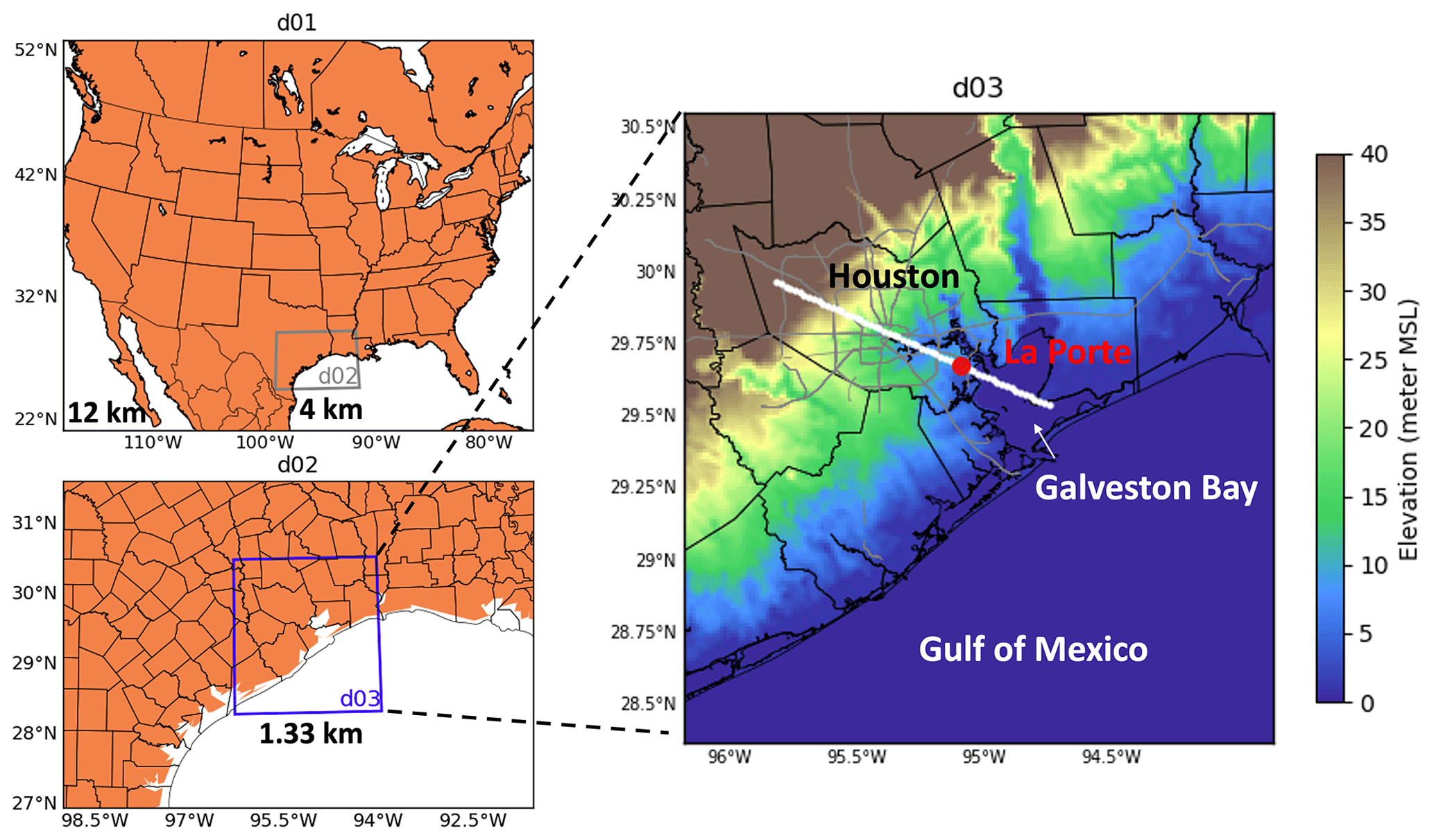
Figure 1WRF-GC nested domains and their horizontal resolutions. The La Porte site is indicated with a red dot. The white line represents a flight track that is chosen because of its proximity to the La Porte site.
WRF-GC uses the most updated full Ox–NOx–volatile organic compound–halogen–aerosol chemistry from GEOS-Chem. The anthropogenic emissions used are the 2019 TCEQ emission inventory for Houston and southeastern Texas, the 2013 National Emission Inventory for the rest of the USA, and the 2014 Community Emissions Data System (CEDS) for regions outside of the USA. Biomass burning emissions are from the 2019 Global Fire Emissions Database (GFED). Biogenic emissions are from the Model of Emissions of Gases and Aerosols from Nature (MEGAN; Guenther et al., 2012). Soil NOx (Hudman et al., 2012) and lightning NOx (Murray et al., 2012) emissions are also included.
2.3.2 Model configurations
Boundary and initial conditions for WRF employed three alternative meteorological analyses. They were (1) the National Centers for Environmental Prediction (NCEP) Final Analysis (FNL; https://rda.ucar.edu/datasets/ds083.3/, last access: 26 September 2023), (2) the fifth generation of European Centre for Medium-Range Weather Forecasts (ECMWF) atmospheric reanalysis (ERA5) data (https://rda.ucar.edu/datasets/ds633.0/, last access: 26 September 2023), and (3) the High-Resolution Rapid Refresh (HRRR) from National Oceanic and Atmospheric Administration (NOAA) Amazon Web Service (AWS; https://registry.opendata.aws/noaa-hrrr-pds, last access: 26 September 2023). The temporal resolution for FNL, ERA5, and HRRR is 6 h, hourly, and hourly, respectively. The horizontal resolution for FNL, ERA5, and HRRR is 0.25∘, 0.25∘, and 3 km, respectively. We used geopotential heights and winds at 850 hPa from the ERA5 dataset to derive synoptic conditions in Fig. 2.
WRF has different schemes or options to represent physics and dynamics processes. Three PBL schemes were used to investigate the effect of different parameterizations of heat, moisture, and momentum exchange between the surface and PBL on the simulated PBL structure and height. They are the local closure Mellor–Yamada–Nakanishi–Niino (MYNN) scheme (Nakanishi and Niino, 2009), the non-local closure Yonsei University (YSU) scheme (Hong et al., 2006), and the hybrid local–nonlocal Asymmetric Convective Model version 2 (ACM2) scheme (Pleim, 2007a, b). Details of the PBL schemes are in Sect. 2.3.3. Two microphysics schemes were used, namely the Morrison double-moment (2M) scheme (Morrison et al., 2009) and the WRF single-moment 6-class (WSM6) scheme (Hong and Lim, 2006). Other schemes adopted in this paper were the Monin–Obukhov similarity surface layer, the Noah land surface scheme (Chen and Dudhia, 2001), the rapid radiative transfer model (RRTM) longwave and shortwave radiation schemes (Iacono et al., 2008), and the new Tiedtke cumulus scheme (Zhang et al., 2011; Tiedtke, 1989).
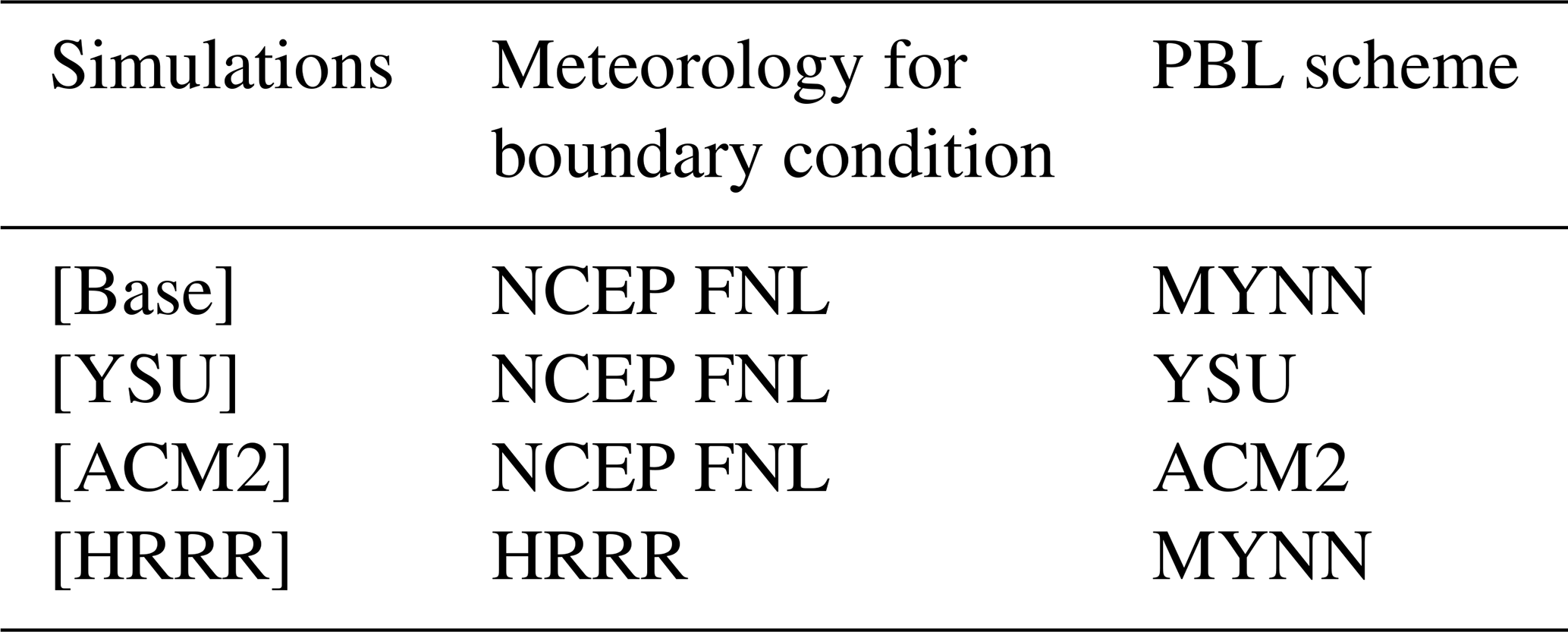
To select the best model configuration to represent meteorology during the 2021 TRACER-AQ campaign, we designed eight model experiments with different physics options, boundary meteorology, data assimilation, and reinitializing option, as listed in Table S2. First, [Base] is the baseline configuration, with MYNN for PBL, 2M for microphysics, NCEP FNL for boundary conditions, no nudging for assimilation, and no reinitialization. Second, [YSU] and [ACM2] experiments used the YSU and ACM2 PBL schemes, respectively, while keeping other options the same as [Base]. Differences between [Base], [YSU], and [ACM2] show the effects of different PBL parameterizations. Third, the [WSM6] experiment differs from [Base] by replacing the 2M microphysics scheme with WSM6. Differences between [Base] and [WSM6] show the effects of different microphysics schemes. Next, [ERA5] and [HRRR] were designed to show the effects of different meteorological initial and boundary conditions on the WRF performance by using ERA5 and HRRR instead of NCEP FNL, respectively. We examined the effects of data assimilation options in [Nudged]. [Nudged] adopted observation nudging and surface analysis nudging to assimilate both onshore and offshore measurements from multiple platforms, including the TCEQ CAMS, boats, and the NCEP surface and upper-air measurements into WRF meteorology (see Sect. S2 for details). Differences between [Base] and [Nudged] show the effects of assimilation. Last, [Reinit] used daily reinitialization, where the simulation was broken into many 30 h segments, with the first 6 h of each segment (18:00–23:00 UTC of a previous day) as spin-up and the subsequent 24 h (00:00–23:00 UTC of the following day) used for analysis (Yahya et al., 2015; Otte et al., 2008). Differences between [Base] and [Reinit] show the effects of a free-running option versus model reinitialization.
The WRF model generally reproduces observed temporal variability and spatial distribution in key meteorological parameters with a correlation coefficient higher than 0.5 in most cases. However, the model, regardless of the configuration settings, shows persistent low biases in PBL heights, low biases in air temperatures, high biases in relative humidity, and high biases in wind speed (see Sect. S3 for details). While different WRF configuration has its own advantage in reducing model biases, [HRRR], [Nudged], and [Reinit] configurations stand out as the three best simulations based on campaign-wide statistics (see Sect. S3 for details). Considering that [Nudged] requires additional efforts to prepare observational datasets and [Reinit] needs to automate the model running process, [HRRR] is the easiest and the most effective option to reproduce meteorology for computationally expensive chemistry simulations and was thus selected to be presented in the analysis below. Meanwhile, the three simulations with different PBL schemes (i.e., [Base], [YSU], and [ACM2]) were also selected because the choice of the PBL scheme is crucial in determining PBL heights (Sect. 2.3.3), which is one of the major interests of this study. Therefore, we chose four simulations, i.e., [HRRR], [Base], [YSU], and [ACM2], in Table 1. The surface layer, land surface, longwave and shortwave radiation, and Tiedtke cumulus schemes remain unchanged in all simulations.
2.3.3 Determination of PBL height in different schemes
Atmospheric models adopt the thermodynamic concept and rely on parameterization schemes to define the structure and the height of the PBL. The heights of the PBL are determined differently among different PBL schemes in the WRF model. The intra-scheme differences can originate from (1) the vertical profile of thermodynamic quantities simulated with different assumptions of the vertical exchange of heat, moisture, and momentum and (2) the diagnosis of the PBL height from these thermodynamic quantities. The PBL heights determined by different schemes can differ by 20 %–30 % (Hu et al., 2010; Xie et al., 2013).
First, the common parameterizations of vertical exchange include local and non-local closure schemes. Local closure schemes estimate the turbulent fluxes at each point in model grids from the mean atmospheric variables and their gradients at that point. In contrast, non-local closure schemes include the nonlocal upward transport by buoyant plumes, representing large-scale motions. Among the three PBL schemes used in this study, the MYNN scheme is local, the YSU is nonlocal, and the ACM2 is hybrid local–nonlocal.
Second, the bulk Richardson number (BRN) and the turbulent kinetic energy (TKE) methods are the two common methods to determine PBL height. The BRN method diagnoses PBL height thermodynamically by the potential temperature with wind speeds and is adopted in the YSU and the ACM2 schemes. The PBL heights under this condition are defined as the height of the model layer at which the bulk Richardson number reaches a critical value. The two schemes have two major differences. The YSU scheme calculates the bulk Richardson number, starting from the surface, while the ACM2 scheme calculates it above the neutral buoyancy level (Hu et al., 2010; Hong et al., 2006; Pleim, 2007a, b). The critical value is 0.25 for stable conditions and 0 for unstable conditions in the YSU scheme, and it is 0.25 for both stable and unstable conditions in the ACM2 scheme (Xie et al., 2013). Meanwhile, the TKE method diagnoses the PBL height by horizontal and vertical winds and is adopted in the Mellor–Yamada–Janjic (MYJ) scheme (not used in this study). The PBL height under this condition is diagnosed when the TKE decreases to a minimum of 0.1 m2 s−2. A hybrid definition that combines the BRN and the TKE methods is implemented in the MYNN scheme. The hybrid method weights the TKE method as being more during stable conditions when the BRN-based PBL height is below ∼0.5 km, while it weights the TKE-based definition as being negligible when the BRN-based PBL height is above ∼1 km.
Previous studies have demonstrated that the aforementioned schemes outperform each other under different conditions across regions when evaluated with various metrics (Hu et al., 2010; Xie et al., 2012, 2013). No conclusion is reached as to which scheme is universally the best. No systematic higher or lower PBL height is expected from one scheme relative to one another.
2.4 Performance metrics for wind
The mean of wind speed and direction is calculated using the vector notation approach, a commonly used method in wind evaluations, as described in Yu et al. (2022). This method treats wind as vectors with their u (eastward) and v (northward) wind components. First, the mean u and v wind components are found by averaging all u and v wind values over a given time period. Then, the resultant vector is determined by taking the square root of the sum of the squares of the mean u and mean v wind components. The magnitude of the resultant vector represents the mean wind speed, and the angle of the resultant vector represents the mean wind direction.
The difference between observed and modeled wind direction was calculated as below.
where M is the model output, and O is the observation. The correlation between observed and modeled wind direction was determined by a circular correlation coefficient as below.
The geopotential heights at 850 hPa in Fig. 2 show different synoptic conditions are seen between ozone episode and clean days in September 2021. The clean days experienced clean southerlies from the Gulf of Mexico (Fig. 2a), while the ozone episodes of 6–11 and 23–26 September both happened after a cold frontal passage, with a low pressure sitting in the northeast USA and a high pressure located in eastern Texas (Fig. 2b and c). This synoptic structure puts the Houston region under northerly wind conditions, which bring colder and more polluted continental air to the region, leading to relatively lower temperatures (Fig. 3a) and relative humidity (Fig. 3b) than clean days.
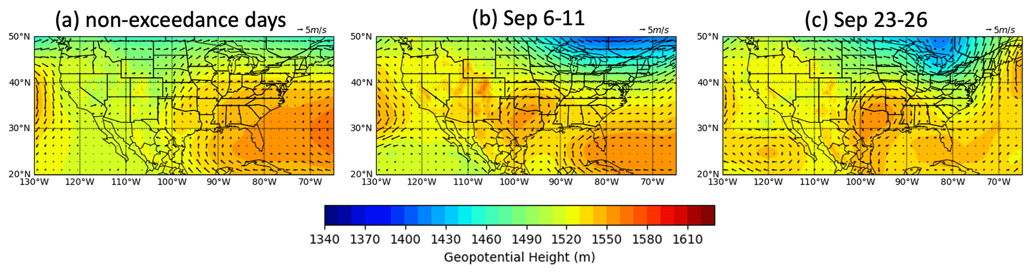
Figure 2Synoptic conditions denoted by geopotential height at 850 hPa and the associated winds for (a) the clean days and the two ozone episodes of (b) 6–11 September and (c) 23–26 September 2021.
Apart from differences in the meteorological variables, synoptic high-pressure centers during ozone episodes tend to create clear, calm conditions, with light horizontal winds at night when the RL and the multiple layer structure of the lower troposphere (including an SBL, an RL, and a CI layer) are prone to form, while the RL structure tends to be disrupted due to shear effects under meteorological conditions during clean days (Stull, 1988; Yi et al., 2001). We find mixed-layer heights derived from the ceilometer at La Porte during clean days and ozone episode are similar during the daytime, while the nocturnal mixed-layer heights (e.g., 00:00–10:00 CDT) are greater on ozone episode days than on clean days (Fig. 3e). Such differences can also be seen from the direct measurements of the ceilometer, e.g., atmospheric backscatter profiles. During ozone episodes, the high-pressure center creates favorable meteorological conditions for multiple nocturnal layers to form. Among these, the RL contains much of the aerosol remnant left by the daytime CBL and is therefore detected by the ceilometer during ozone episodes (Fig. 3f). In contrast, no such multiple layers form under meteorological conditions on clean days. Much of the aerosol remnant above the SBL is dissipated with the disruption of RL by wind shear, such that the SBL contains more aerosol than above. Therefore, the ceilometer detects the SBL on clean days (Fig. 3f). In this study, the mixed-layer heights derived from the ceilometer represent the RL during ozone episodes but the SBL during clean days.
Mixed-layer height is often a good proxy for the heights of different lower-tropospheric layers determined thermodynamically in models (Scarino et al., 2014; Kuik et al., 2016; Haman et al., 2014). We refer to the standard mixed-layer retrievals, including the CBL during the daytime, the SBL at night during clean days, and the RL at night during ozone episodes, respectively, as observed in the CBL, SBL, or RL (hereafter in a manner consistent with the modeled equivalents).
Based on the observed differences in diurnal PBL variations between clean days and ozone episodes in Sect. 3, we first assessed the observation–model differences in diurnal variation in the PBL heights and other meteorological variables in Sect. 4.1. The ground-based ceilometer at the La Porte site is used to evaluate the diurnal variation due to its capability for continuous measurements throughout the day. Meanwhile, the HSRL-2 instrument provides data covering a significant portion of the urban Houston region and adjacent waters and is thus used to evaluate spatial and temporal (daytime) variations in the PBL heights in Sect. 4.2.
4.1 Evaluation with ceilometer
Figure 3 compares the diurnal variations in the PBL height between clean days and ozone episode days. During the daytime, the observations represent the CBL height for both types of days. This aligns with the standard model output for the PBL height during the daytime, which is the CBL height. At night, the observations represent the SBL height on clean days, whereas they represent the RL height on ozone episode days. However, the model only provides the SBL as the standard output for nighttime PBL, lacking information on other nocturnal layers such as RL. As a result, meaningful comparisons between the observed RL height and the modeled SBL height during ozone episodes become challenging. Therefore, the modeled RL needs to be extracted for a fair comparison against the observed RL during ozone episodes.
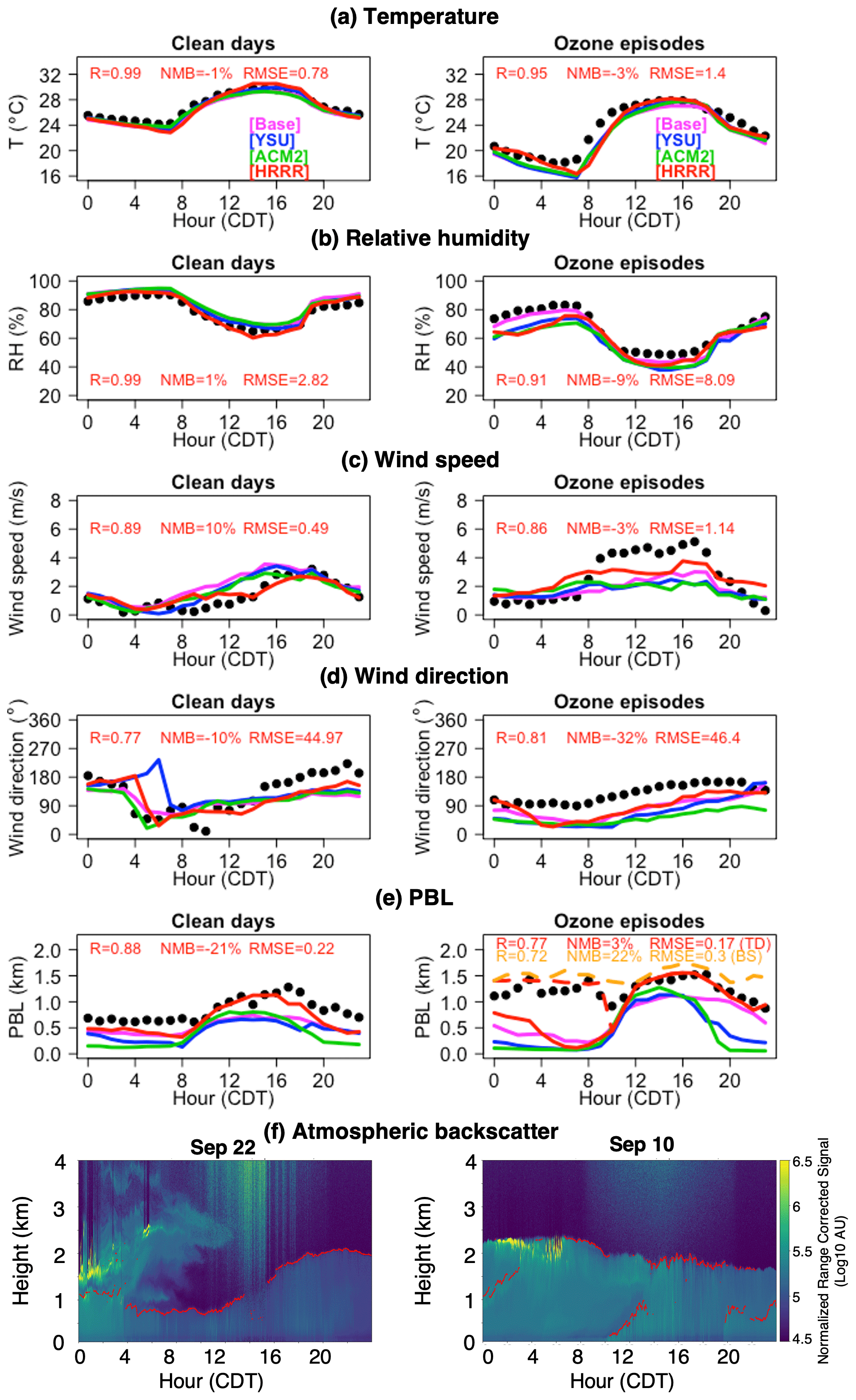
Figure 3Diurnal variations in observed versus modeled surface meteorology and PBL height averaged over clean periods (left) and ozone episodes (right) in September 2021. In panels (a)–(e), black dots are NASA GSFC observations at the La Porte site, while the lines are model equivalents of different configurations of WRF-GC. In panel (e), dashed lines represent residual layers identified by aerosol backscatter (BS) versus thermodynamically by potential temperature (TD) from the [HRRR] configuration. Panel (f) shows the ceilometer-measured atmospheric backscatter profiles overlaid with mixed-layer heights of a clean day of 22 September and an ozone episode day of 10 September.
We first selected [HRRR] as the best simulation among the four simulations, according to their daytime performances for both types of days. On clean days, the model simulations show the diurnal mean and standard deviation of the PBL height of 0.52±0.14 km for [Base], 0.43±0.17 km for [YSU], 0.39±0.27 km for [ACM2], and 0.66±0.28 km for [HRRR] in comparison with the observed value of 0.83±0.22 km (left panel of Fig. 3e). On ozone episode days, the model simulations show the CBL height variation of 0.96±0.18 km for [Base], 0.60±0.37 km for [YSU], 0.50±0.5 km for [ACM2], and 1.25±0.29 km for [HRRR] in comparison with the observed value of 1.26±0.24 km during the afternoon and evening hours of 15:00–23:00 CDT (right panel of Fig. 3e). During the same period, the model simulations show the PBL decay rates of 53 m h−1 for [Base], 102 m h−1 for [YSU], 135 m h−1 for [ACM2], and 59 m h−1 for [HRRR] in comparison with the observed 60 m h−1. These comparisons demonstrate that the four model simulations generally underestimate the PBL height by 180–450 m throughout the day on clean days and by 10–760 m during the daytime on ozone episode days. Among the four simulations, [HRRR] best captures the observed mean height and decay rate during the daytime. Therefore, [HRRR] is selected to display its aerosol backscatter and potential temperature profiles in Figs. 4 and 5, thus enabling further examination of its representation of the nighttime RL.
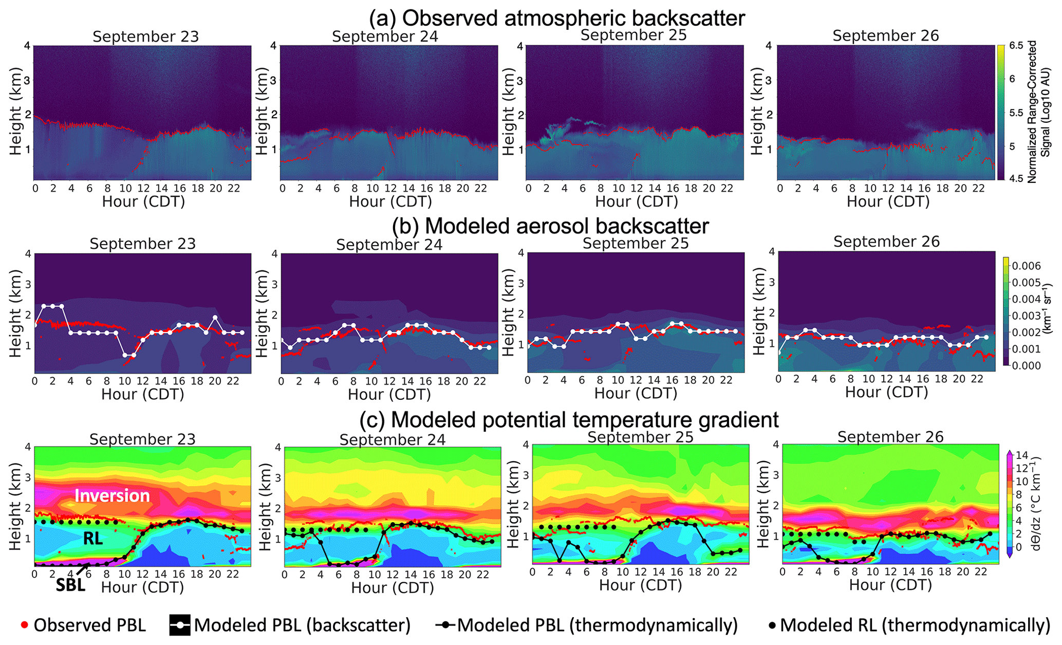
Next, the simulated aerosol backscatter and potential lapse rates of the [HRRR] simulation are used to extract the modeled RL heights. The modeled aerosol backscatter shows the volume of the atmosphere in which aerosol species are mixed and dispersed. Substantially stronger backscatter signals are found within the first ∼2 km than in the free troposphere at 3–4 km aloft (Figs. 4b, 5b). Therefore, we take the sharpest vertical gradient in the backscatter signal (i.e., the largest first derivative of backscatter) to estimate the modeled mixed-layer height. The extracted layers have daytime variations of 1.58±0.13 km and nighttime variations of 1.50±0.06 km during ozone episodes. Such nighttime variations are representative of the RL top in the model. It is worth noting that the modeled aerosol backscatter in Figs. 4b and 5b is not equivalent to the ceilometer-measured atmospheric backscatter in Figs. 4a and 5a, which includes both aerosol and molecular backscatter signals. Yet this modeled aerosol backscatter is the closest product from the model and denotes relatively consistent backscatter differences above and below the RL.
Apart from aerosol backscatter, the potential lapse rate is also commonly used to distinguish atmospheric layers according to their instability. The potential lapse rate or potential temperature gradient is thermodynamically defined as the change in the potential temperature (θ) with height (z). Distinguished by the values of the potential lapse rate, the modeled nocturnal PBL consists of a stable SBL, a neutrally stratified RL, and a CI layer during most ozone episode days (Figs. 4c, 5c). The modeled top of the RL can be identified from the height at which the RL (with little or low temperature increases at 0–3 ∘C km−1) transitions to the CI layer (with drastic temperature increases at 8–14 ∘C km−1). Therefore, we use the sharpest gradient in the potential lapse rate, which is 6.6 ∘C km−1 on average, to identify the top of the modeled RL. This thermodynamically identified top of the RL exhibits a variation of 1.39±0.03 km during ozone episodes, which is slightly lower than the 1.50±0.06 km identified by the aerosol backscatter in the previous paragraph.
The modeled PBL heights identified by the two methods above show reasonable agreement with the observed PBL heights measured by the ceilometer. Such a comparison can be found in Fig. 3e. The thermodynamically identified layer exhibits a slightly better agreement with the observation, exhibiting a correlation coefficient (R) of 0.77, a normalized mean bias (NMB) of 3 %, and a root mean square error (RMSE) of 0.17 km. In contrast, the backscatter-identified layer shows slightly lower correlation and larger biases (R=0.72; NMB = 22 %; RMSE = 0.30 km) during ozone episodes.
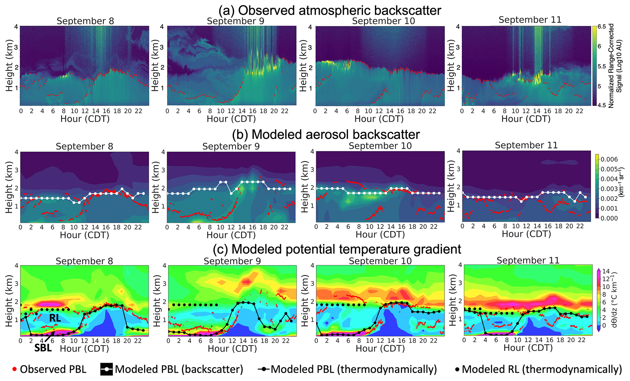
Figure 4Observed and modeled heights of lower-tropospheric layers at the La Porte site during the ozone episode of 8–11 September. The contours show the (a) ceilometer-observed attenuated atmospheric backscatter signal produced by aerosols and molecules combined at 1064 nm, (b) modeled unattenuated backscatter of aerosols alone at 1000 nm, and (c) modeled potential temperature gradient. Red dots are ceilometer-observed mixed layers. White and black lines are backscatter-defined and thermodynamically defined mixed layers from the [HRRR] model simulation.
4.2 Evaluation with HSRL-2
Section 4.1 above evaluated the model performance in continuous temporal variations using a ground-based ceilometer at the La Porte coastal site. In this section, our focus shifts to assessing the spatial variations in the modeled PBL heights by comparing them with the airborne HSRL-2 mixed-layer heights. The HSRL-2 conducted measurements over the Houston region and the adjacent Galveston Bay, typically 3 times per day on 8 high-ozone days and 2 clean days in September 2021. As mentioned in the previous sections, the mixed layer can represent the PBL under various conditions. Therefore, from this point onwards, we refer to the observed mixed-layer heights as observed PBL heights to maintain consistency with the modeled equivalents.
During ozone episodes over land in the urban Houston region, the observed PBL heights gradually increase from 0.63±0.25 km in the morning (08:00–10:00 CDT) to 1.27±0.38 km at noon (11:00–13:00 CDT) and further to 1.69±0.23 km in the afternoon (14:00–16:00 CDT). Compared to land, the higher heat capacity in water leads to slower heating and cooling, resulting in a more stable atmosphere and shallower PBL. Over Galveston Bay, the observed heights are consistently lower by around 0.13–0.26 km during the three measured time periods. Such daytime variation and land–water differences can be observed on a specific high-ozone day of 9 September in Fig. 6. In comparison with these observations above, the four model simulations underestimate the PBL heights to different extents (NMB from −3 % to −62 %; RMSE from 0.22 to 0.81 km) in Table 2. The model exhibits notably lower performance on land in the morning than under other conditions, showing less correlation and larger biases. This is because the morning mixed-layer heights on land during ozone episodes can be difficult to retrieve with the influences from multiple layers (e.g., SBL and RL), and they can differ substantially from the thermodynamically defined PBL from the model. Therefore, we do not expect the model to capture the spatial patterns of mixed-layer heights on land in the morning. Excluding this special case of morning PBL on land, we found that [HRRR] exhibits a higher correlation (R=0.26–0.68) and lower biases (NMB from −3 % to −21 %; RMSE from 0.22 to 0.46 km) in most cases during ozone episodes.
During clean days, the observed PBL height increases from 0.78±0.14 km in the morning to 1.07±0.24 km at noon over land and slightly from 0.57±0.28 km in the morning to 0.65±0.34 km at noon over water. The model captures such variations during clean days less effectively, resulting in lower correlation and larger biases compared to ozone episodes (Table 2). One important reason for the lower model performance during clean days compared to ozone episodes is the substantial difference in the number of data points collected. There are significantly fewer data points available during the 2 clean days compared to the 8 high-ozone days (Table 2).
The above analysis indicates that under both high-ozone and clean days, the four model simulations consistently underestimate the observed PBL heights under most conditions. Next, we will investigate the model performances in simulating land–water differences.
The observed land–water differences in PBL heights are larger in the afternoon than in the morning during both ozone episode and clean days. During noon and afternoon hours of ozone episodes, the model exhibits better performance in capturing the heights of the PBL on land than over water. This is expected, as the model's physics parameterization is likely better tuned and calibrated for land surfaces for which more observations are available compared to water. During the same period, the observed mean land–water differences of 0.13 km (noon) and 0.26 km (afternoon) are predicted to be larger in the model with values of 0.32–0.52 km (noon) and 0.44–0.56 km (afternoon), respectively. This is because the model shows consistently smaller underestimations over land than water during this period. During clean days, the observed land–water gradients of 0.21 km (morning) and 0.42 km (noon) are simulated to be 0.14–0.22 km (morning) and 0.36–0.76 km (noon), respectively. The [ACM2] and the [HRRR] slightly outperform the other two simulations for land–water differences (Table 2).
Table 2Statistics of the observed HSRL-2 mixed-layer height and the modeled thermodynamic PBL height during ozone episode days (8–10 and 23–26 September) and clean days (1 and 3 September). Morning, noon, and afternoon are defined as 08:00–10:00, 11:00–13:00, and 14:00–16:00 CDT. Land and water are defined by the gray boxes in Fig. 6. The correlation coefficient (R) and normalized mean bias (NMB) are unitless. The root mean square error (RMSE) has the same unit as PBL height in kilometers.
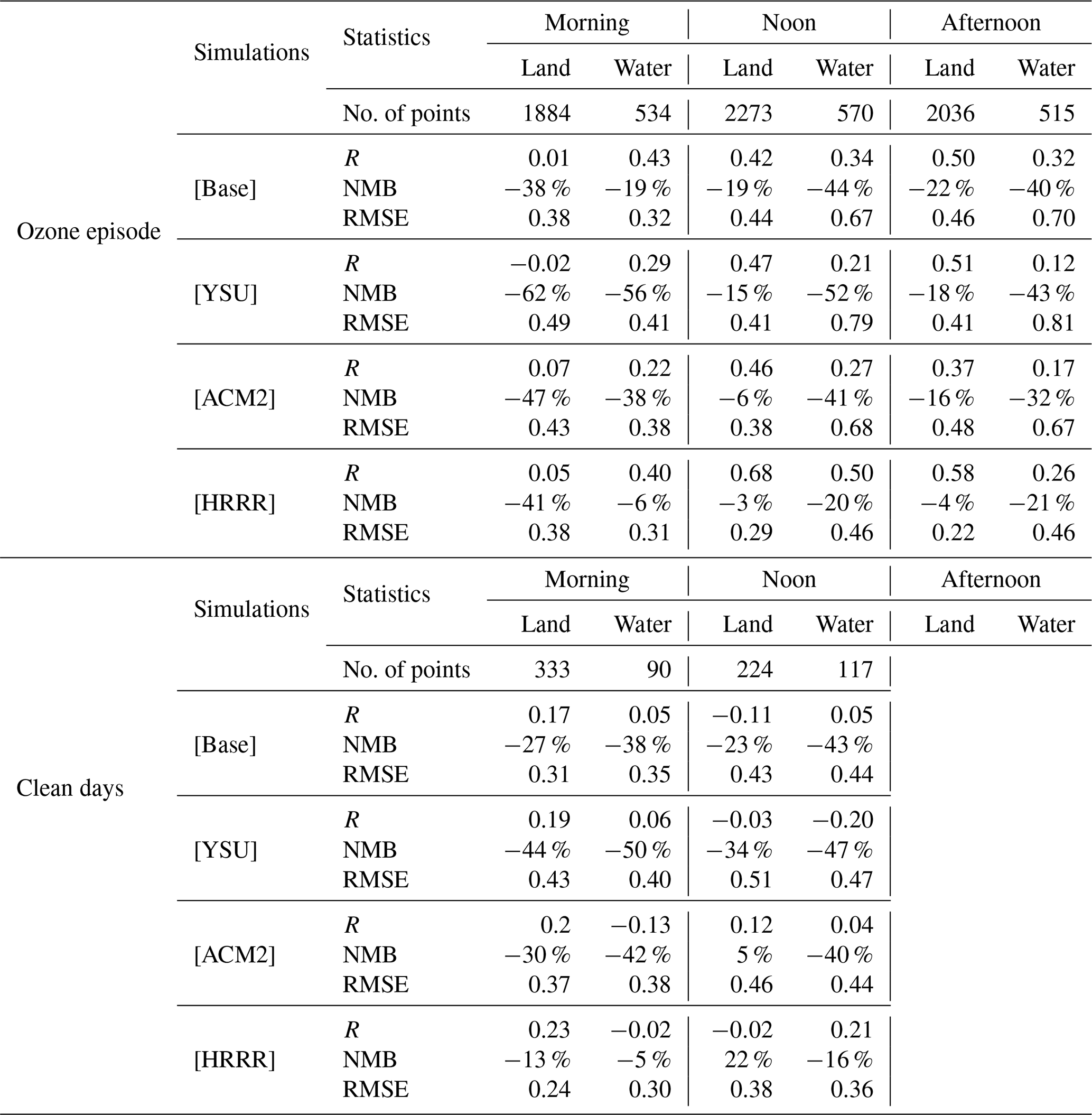
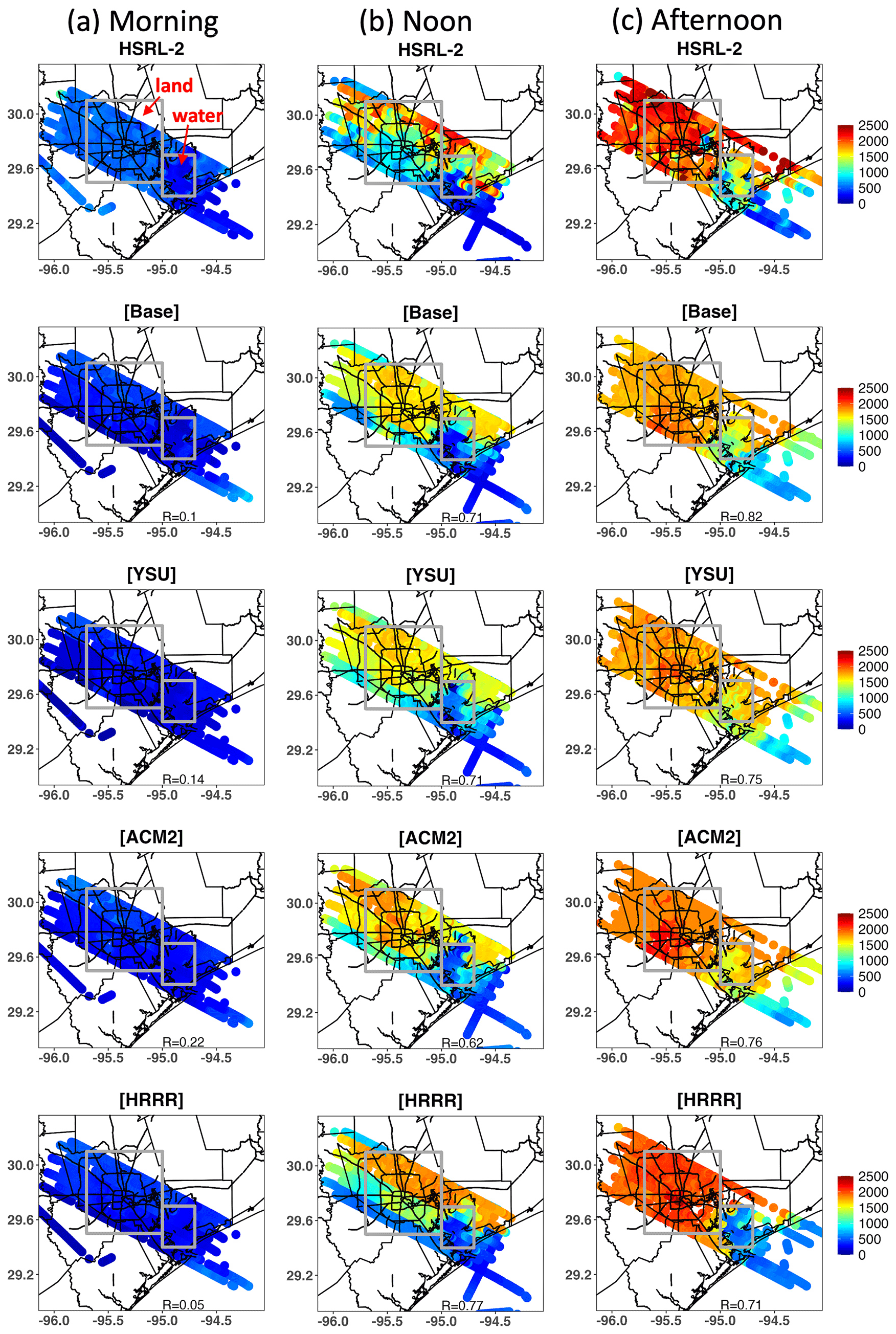
Figure 6Spatial variabilities in the PBL heights (in meters) from the HSRL-2 and different WRF-GC simulations (a) in the morning (08:00–10:00 CDT), (b) at noon (11:00–13:00 CDT), and (c) in the afternoon (14:00–16:00 CDT) of 9 September 2021.
Boundary layer mixing can bring air aloft towards the surface, and vice versa, leading to an uneven vertical distribution of ozone which accordingly affects surface ozone concentrations. This section uses independent field measurements at La Porte (including TROPOZ, HSRL-2, ozonesondes, a model 49i ozone analyzer, and a CAMS site named La Porte Sylvan Beach) to validate the modeled vertical ozone profiles at three layers, including the lower free troposphere (2–3 km aloft), the boundary layer (0.5–1 km aloft), and the ground level (<50 m). Since the [HRRR] simulation best represents the PBL heights in Sect. 4, it is used to investigate vertical ozone profiles in this section.
5.1 Free tropospheric ozone entrainment
The strength of the CI layer regulates the gas exchange between the FT and the PBL. Strong convection can penetrate a weak CI layer and entrain FT air into the PBL (i.e., entrainment), while a strong CI layer acts as a lid to restrict gas exchange between the PBL and the FT. The potential temperature differences between the top and bottom of the CI layer are often used to indicate the strength of the CI layer and the extent of entrainment processes (Kaser et al., 2017; Morris et al., 2010; Rappenglück et al., 2008). We first identified the modeled CI layers at 1.5–3 km aloft during ozone episodes in Figs. 4c and 5c and then calculate the temperature differences in the model between the top and bottom of the CI layers on each day. The corresponding daily inversion strength is 2.3, 2.8, 6.8, and 6.4 ∘C during 8–11 September and 13.6, 7.5, 7.8, and 8.4 ∘C during 23–26 September, respectively. Among these days, 8 and 9 September experienced the weakest inversions. To examine if the modeled inversion strength is representative of the observations, we evaluate the modeled potential temperature profiles with ozonesonde measurements in Fig. 7a. Results show that the model simulates the vertical profiles of potential temperature well across different days, with high correlation (R=0.99) and low biases (NMB from 0 % to −2 %; RMSE from 0.92 to 1.30 ∘C).
Combining the inversion strengths (Figs. 4c, 5c) and the vertical ozone distributions from the TROPOZ lidar (Fig. 8a and d) helps to identify the potential entrainment of the FT air into the underlying PBL on 8 and 9 September at the La Porte site. On 8 September, strong convection associated with a rapid CBL growth penetrates the thin and weak inversion at 2 km aloft at around noon (Fig. 4c) and allows the ozone-rich air above to entrain into the CBL, adding to afternoon ozone buildup (Fig. 8a). Similarly, there is no CI layer present overnight from 20:00 CDT on 8 September to 10:00 CDT on 9 September (Fig. 4c) and thus long-lasting ozone entrainment into the RL (Fig. 8a). Conversely, a strong and thick inversion at 1.5–3 km decouples the FT and the underlying PBL during 23–24 September (Fig. 5c) and the ozone layer remains aloft at 2–3 km (Fig. 8d). The inversion strength presented here is one way to approach the potential entrainment, and follow-up studies can probe into the detailed dynamics. It is also noteworthy that the presented vertical distribution of ozone is also largely shaped by local ozone production in the boundary layer. Since this study is focused on the vertical ozone distribution impacted by mixing between lower- free-tropospheric layers, the vertical ozone distribution impacted by chemistry and differentiating between the contributions from dynamics and chemistry are outside the scope of this analysis.
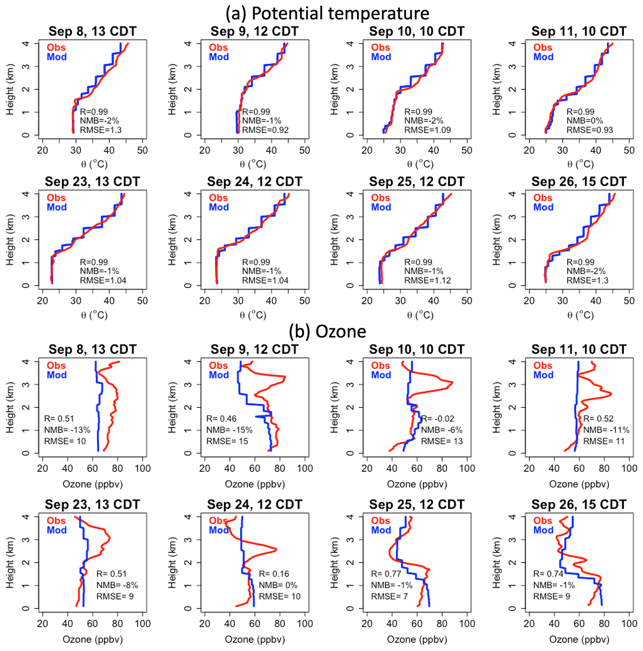
Figure 7Vertical profiles of (a) potential temperature and (b) ozone from ozonesonde measurements and the WRF-GC [HRRR] simulation at La Porte during 8–11 and 23–26 September.
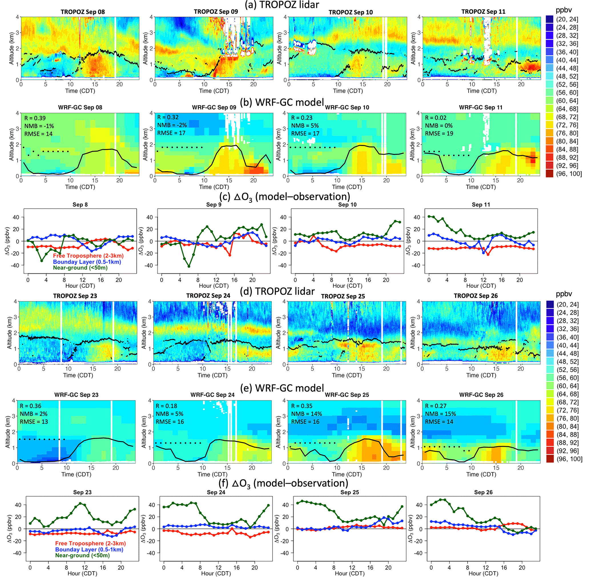
Figure 8Time series of the vertical ozone profile from the TROPOZ ozone lidar (a, d) and the WRF-GC [HRRR] simulation (b, e) at La Porte. Observed and modeled boundary layer heights are inserted, respectively. Dots represent the modeled residual layer identified in this study. Line plots (c, f) show ozone differences (model minus observation) at the free troposphere (2–3 km) and the boundary layer (0.5–1 km) from the TROPOZ, as well as the near-ground (<50 m) from the model 49i ozone analyzer.
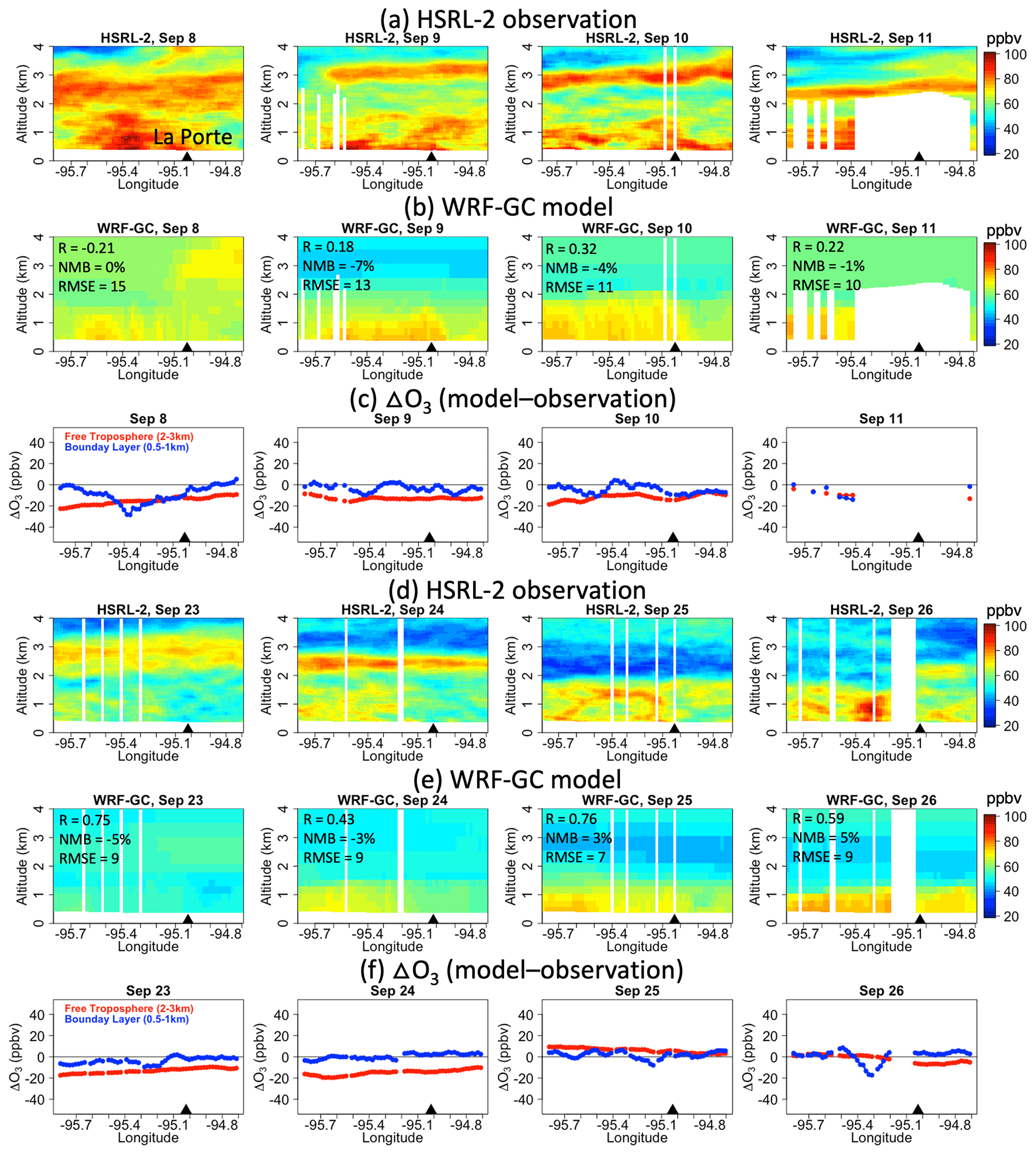
Figure 9Vertical ozone profiles from (a, d) the HSRL-2 and (b, e) the WRF-GC [HRRR] simulation. The profiles are taken from a flight track (Fig. 1) over urban Houston and Galveston Bay at around 11:00–13:00 CDT each day. Line plots (c, f) show ozone differences (model minus observation) at the free troposphere (2–3 km) and the boundary layer (0.5–1 km).
5.2 Evaluation of ozone vertical distribution
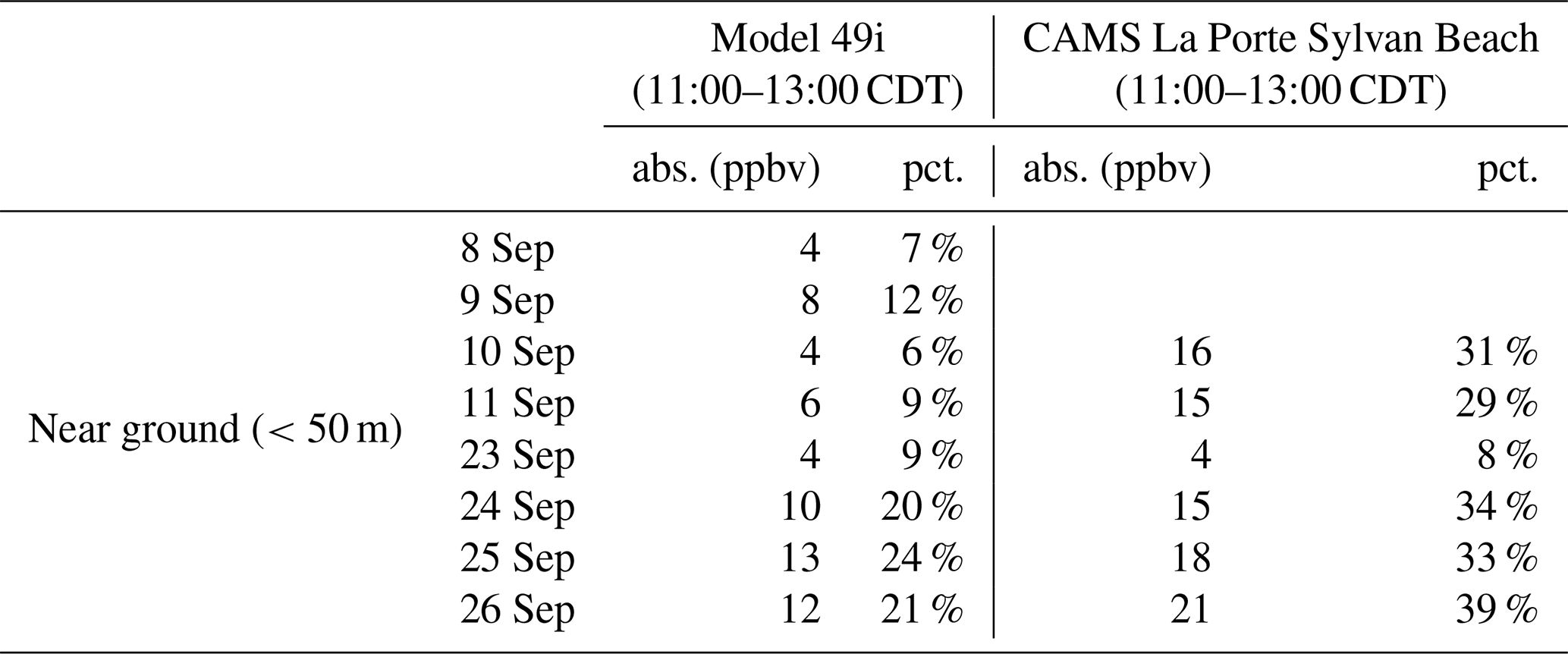
Multiple field measurements at La Porte are used to evaluate the modeled vertical ozone distribution at the free troposphere (2–3 km), the boundary layer (0.5–1 km), and the near-ground level (<50 m). According to data availabilities at different levels, the free troposphere and boundary layer are evaluated by the TROPOZ, the HSRL-2, and ozonesondes (Table 3), while the ground level is evaluated by a model 49i ozone analyzer and a CAMS site named La Porte Sylvan Beach (Table 4). To cross-compare among multiple measurements, we present the model–observation differences at a common site (La Porte) during a common time slot (11:00–13:00 CDT). Larger ozone differences are found at the near-ground level than for the boundary layer and lower free troposphere (Tables 3 and 4).
As shown in Table 3, the model underestimates the layer of enhanced ozone at 2–3 km aloft in the free troposphere by 9 %–21 % (TROPOZ), 15 %–22 % (HSRL-2), and 14 %–22 % (ozonesondes) at La Porte at 11:00–13:00 CDT during 8–11 and 23–24 September. Unlike most of the campaign's ozone-exceedance days, 25 and 26 September do not have an enhanced ozone layer at 2–3 km aloft but have a lower ozone layer relative to the background tropospheric values instead; this low-ozone layer is overestimated by 9 %–12 % on 25 September but underestimated by 3 %–12 % on 26 September. Meanwhile, the model underestimates the boundary layer ozone at 0.5–1 km aloft by 6 %–10 % (TROPOZ), 6 %–12 % (HSRL-2), and 1 %–11 % (ozonesondes) during the first ozone episode of 8–11 September but overestimates it by 0 %–6 % (TROPOZ), 3 %–5 % (HSRL-2), and 5 %–7 % (ozonesondes) during the second episode of 23–26 September. The above model–observation differences are based on the common site (La Porte) and common time (11:00–13:00 CDT) among different measurements; the temporal (Fig. 8c and f) and spatial (Fig. 9c and f) variations in these differences are shown in Figs. 8 (TROPOZ) and 9 (HSRL-2).
While free-tropospheric and boundary layer ozone are important components of the vertical ozone distribution due to their thickness, the thin layer of near-ground ozone affects human and vegetation health the most and thus receives more attention. In Table 4, the model overestimates near-ground ozone by 6 %–24 % (model 49i ozone analyzer) and 8 %–39 % (CAMS La Porte Sylvan Beach) at La Porte at 11:00–13:00 CDT during the two ozone episodes. Figure 8c and f show the temporal variations in the model–observation differences from the model 49i ozone analyzer. Most near-ground ozone differences occur at night, consistent with the known problem of overestimating nighttime ozone common to many photochemical models (Schnell et al., 2015; Travis et al., 2016; Jaffe et al., 2018). The WRF-GC model adopts a chemical module from GEOS-Chem. Thus, the two share the difficulties in replicating nighttime ozone due to reasons such as the insufficient representation of the stratification of multiple nocturnal atmospheric layers, uncertainties in gas exchanges between the residual layer and the underlying surface layer, and difficulties in simulating the timing of changes in PBL dynamics (Travis and Jacob, 2019).
To assess vertical variations below the first 4 km, we present performance metrics in Fig. 7 for ozonesondes, Fig. 8 for TROPOZ, and Fig. 9 for HSRL-2. Different comparisons between observations and the model reflect distinct aspects. For instance, comparisons with ozonesondes pertain to vertical variations at a fixed location and time (R=0.46–0.77; NMB from −1 % to −15 %; RMSE = 7–15 ppbv). This emphasis on a specific aspect explains why the correlation is higher when compared to TROPOZ and HSRL-2, which encompass a broader range of variations. Comparisons with TROPOZ relate to vertical and temporal variations at a fixed location (R=0.18–0.39; NMB from −2 % to 15 %; RMSE = 13–17 ppbv). Comparisons with HSRL-2 represent a combination of vertical, temporal, and spatial variations (R=0.18–0.76; NMB from −7 % to 5 %; RMSE = 7–13 ppbv). The above statistics exclude one or two extreme cases in each observation. Despite the differences in correlation resulting from the diverse representations of variations, biases are similar when compared to the three different observations.
Table 3Absolute (abs.) and percentage (pct.) ozone differences between field measurements and the model at the free troposphere and boundary layer at La Porte.
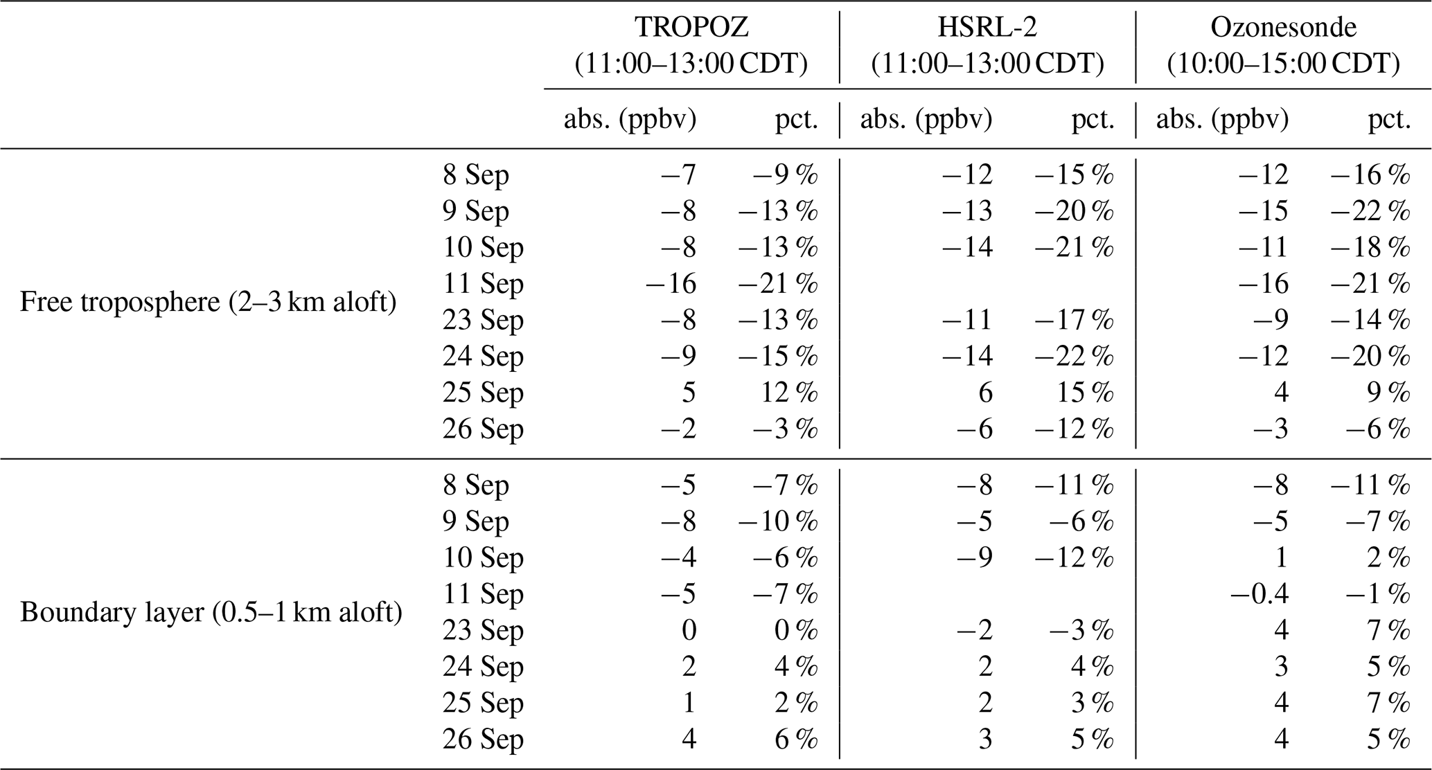
Table 4Absolute (abs.) and percentage (pct.) ozone differences between field measurements and the model at the near-ground level at La Porte.
We used ground-based and aircraft observations collected during the TRACER-AQ campaign in September 2021 to evaluate WRF-GC simulation of the PBL height and ozone in Houston, including two ozone episodes characterized by MDA8 ozone exceeding 70 ppbv. The combined suite of ground-based and airborne meteorological and chemical observations is critical in thoroughly evaluating the spatial and temporal variations in the PBL heights and vertical ozone distributions during multi-day ozone episodes, as presented in this work.
The modeled PBL heights are evaluated with mixed-layer heights retrieved by the ground-based ceilometer and the airborne HSRL-2. Compared with both observations, the four model simulations of [Base], [YSU], [ACM2], and [HRRR] generally underestimate the PBL heights. When compared with the ceilometer, the [HRRR] captures the diurnal variations during clean days (R=0.88; NMB = −21 %; RMSE = 0.22 km). Standard models do not diagnose RL heights, unlike ceilometers. Therefore, we separately identified the modeled RL, following the practices using aerosol backscatter signals and potential temperature gradients during the ozone episodes. As a result, the diurnal variation in the thermodynamically identified layer (R=0.77; NMB = 3 %; RMSE = 0.17 km) compares slightly better than that of the backscatter-identified layer (R=0.72; NMB = 22 %; RMSE = 0.30 km) during ozone episodes. Meanwhile, when compared with the HSRL-2, the [HRRR] exhibits a higher correlation (R=0.26–0.68) and lower biases (NMB from −3 % to −21 %; RMSE = 0.22–0.46 km) than other simulations during noon and afternoon hours during ozone episodes. For land–water differences in PBL heights, the water has shallower PBL heights compared to land. The model predicts larger land–water differences than observations because the model consistently underestimates PBL heights over land compared to water.
We evaluated the vertical ozone distribution with multiple field measurements, including TROPOZ, HSRL-2, ozonesondes, a model 49i ozone analyzer, and a CAMS site named La Porte Sylvan Beach. First, individual evaluations were conducted at the following three lower-tropospheric layers: the free troposphere (2–3 km aloft), the boundary layer (0.5–1 km aloft), and the ground level (<50 m aloft). Results show that the model underestimates the high-ozone layer in the free troposphere by 9 %–21 % (TROPOZ), 15 %–22 % (HSRL-2), and 14 %–22 % (ozonesondes) on most ozone episode days. The boundary layer ozone is underestimated by 6 %–10 % (TROPOZ), 6 %–12 % (HSRL-2), and 1 %–11 % (ozonesondes) during 8–11 September but is overestimated by 0 %–6 % (TROPOZ), 3 %–5 % (HSRL-2), and 5 %–7 % (ozonesondes) during 23–26 September. Meanwhile, the model overestimates near-ground ozone by 6 %–24 % (model 49i ozone analyzer) and 8 %–39 % (CAMS La Porte Sylvan Beach) during the two ozone episodes. Second, we assessed vertical variations in the ozone below the first 4 km through comparisons with TROPOZ, HSRL-2, and ozonesondes. The correlation is higher when compared to ozonesondes than TROPOZ and HSRL-2, as ozonesondes emphasize a specific aspect of vertical variations at a fixed location and time, while the other two encompass a broader range of variations with temporal and spatial variations included. Despite the differences in correlation resulting from the diverse representations of variations, biases shown by these three comparisons are similar.
Based on these evaluations, we summarized the model limitations that prevent a more accurate simulation of PBL heights and the vertical ozone distribution during TRACER-AQ. The first limitation is the single-layer PBL representation. The WRF model only diagnoses the SBL at night, despite the model simulating different physical and thermodynamic properties of multiple nocturnal layers above the SBL. For example, the RL is not identified by the model as a standard diagnosis; this prevents the direct comparison of the model outputs with the observed RL at night. Further efforts are needed to identify and incorporate the RL into the model's standard outputs. Alternative modules aimed at identifying the PBL using simulated vertical backscatter gradients can also enhance the validation of PBL heights with backscatter-derived observations. The second limitation is the underestimation of the layer of enhanced ozone 2–3 km aloft in the free troposphere that was often present on ozone episode days during the campaign. Given its height of 2–3 km and a lifetime of around a week, the layer of enhanced ozone was likely transported into Houston by synoptic flows of cold fronts from the north. The underrepresentation of the synoptic layer of enhanced ozone affects model representations across regions horizontally and atmospheric layers vertically, making it particularly important to model vertical ozone distributions and the effects of entrainment accurately.
Our findings have implications for the predictivity of ozone's vertical mixing and distribution across different modeling systems. For example, WRF is widely used in various meteorology–chemistry coupling systems with different treatments of boundary layer mixing. In WRF-Chem, boundary layer mixing in the chemistry part uses a mixing coefficient originating in WRF, such that the boundary layer mixing calculations in the meteorology and chemistry parts share the same set of coefficients. In WRF-GC, the chemistry part from GEOS-Chem only takes the PBL height from WRF as the maximum height for boundary layer mixing but conducts independent calculations of boundary layer mixing using its own internal methods, which are not reliant on WRF. Unlike online coupled WRF-Chem and WRF-GC, WRF is offline coupled to the Comprehensive Air Quality Model with Extensions (CAMx) in the WRF-CAMx system, and the boundary layer mixing in the chemistry part of CAMx is subject to WRF output frequency instead of the native transport time step in WRF. Considering these distinct treatments of boundary layer mixing in models, the single-layer PBL representation can have varying impacts on the simulation of vertical mixing and, consequently, the vertical distribution of ozone and other air pollutants. Thus, it is essential to understand the differences in boundary layer mixing among different meteorology–chemistry coupling systems. Follow-up studies to this work will address these aspects with a detailed analysis of vertical mixing processes in various models.
WRF-GC is a free and open-source model (https://doi.org/10.5281/zenodo.4395258; Lin, 2020). The two parent models, WRF and GEOS-Chem, are also open source and can be obtained from their developers at https://github.com/wrf-model/WRF (last access: 29 May 2023) and http://www.geos-chem.org (last access: 29 May 2023), respectively.
All observation datasets, model configuration files, model boundary conditions, model input files, and scripts used in this paper are archived in Zenodo (https://doi.org/10.5281/zenodo.7983449, Liu, 2023).
The supplement related to this article is available online at: https://doi.org/10.5194/gmd-16-5493-2023-supplement.
XL and YW conceived the research idea. XL wrote the initial draft of the paper and performed the analyses and model simulations. JF, TG, and SA provided the shipborne data. JTS, MR, and LT provided the TROPOZ and ceilometer data. PW and JTS provided the ozonesonde data. JWH, TS, AJS, and MF provided the HSRL-2 data. All authors contributed to the interpretation of the results and the preparation of the paper.
The contact author has declared that none of the authors has any competing interests.
The findings, opinions, and conclusions are the work of the author(s) and do not necessarily represent the findings, opinions, or conclusions of the AQRP or the TCEQ.
Publisher's note: Copernicus Publications remains neutral with regard to jurisdictional claims in published maps and institutional affiliations.
The authors acknowledge TCEQ for providing the hourly wind, temperature, relative humidity, and MDA8 ozone data and the NASA Langley Atmospheric Science Data Center for providing the TRACER-AQ data archive. We thank Richard Ferrare for helpful suggestions on this paper.
This research has been supported by the Texas Commission on Environmental Quality (TCEQ; grant no. 582-22-31544-019) and by a grant from the Texas Air Quality Research Program (AQRP; grant no. 22-008) at The University of Texas at Austin through the Texas Emission Reduction Program (TERP) and the TCEQ.
This paper was edited by Leena Järvi and reviewed by two anonymous referees.
Angevine, W., Senff, C., and Westwater, E.: Boundary layers/Observational Techniques-Remote, in: Encyclopedia of Atmospheric Sciences, edited by: Holton, J. R., Academic Press, Oxford, 271–279, https://doi.org/10.1016/B0-12-227090-8/00089-0, 2003.
Banta, R. M., Senff, C. J., Nielsen-Gammon, J., Darby, L. S., Ryerson, T. B., Alvarez, R. J., Sandberg, S. R., Williams, E. J., and Trainer, M.: A bad air day in Houston, B. Am. Meteorol. Soc., 86, 657–669, https://doi.org/10.1175/bams-86-5-657, 2005.
Banta, R. M., Senff, C. J., Alvarez, R. J., Langford, A. O., Parrish, D. D., Trainer, M. K., Darby, L. S., Hardesty, R. M., Lambeth, B., Neuman, J. A., Angevine, W. M., Nielsen-Gammon, J., Sandberg, S. P., and White, A. B.: Dependence of daily peak O3 concentrations near Houston, Texas on environmental factors: wind speed, temperature, and boundary-layer depth, Atmos. Environ., 45, 162–173, https://doi.org/10.1016/j.atmosenv.2010.09.030, 2011.
Bernier, C., Wang, Y., Estes, M., Lei, R., Jia, B., Wang, S., and Sun, J.: Clustering Surface Ozone Diurnal Cycles to Understand the Impact of Circulation Patterns in Houston, TX, J. Geophys. Res.-Atmos., 124, 13457–13474, https://doi.org/10.1029/2019jd031725, 2019.
Bernier, C., Wang, Y., Gronoff, G., Berkoff, T., Knowland, K. E., Sullivan, J. T., Delgado, R., Caicedo, V., and Carroll, B.: Cluster-based characterization of multi-dimensional tropospheric ozone variability in coastal regions: an analysis of lidar measurements and model results, Atmos. Chem. Phys., 22, 15313–15331, https://doi.org/10.5194/acp-22-15313-2022, 2022.
Bodini, N., Lundquist, J. K., and Newsom, R. K.: Estimation of turbulence dissipation rate and its variability from sonic anemometer and wind Doppler lidar during the XPIA field campaign, Atmos. Meas. Tech., 11, 4291–4308, https://doi.org/10.5194/amt-11-4291-2018, 2018.
Bonin, T. A., Newman, J. F., Klein, P. M., Chilson, P. B., and Wharton, S.: Improvement of vertical velocity statistics measured by a Doppler lidar through comparison with sonic anemometer observations, Atmos. Meas. Tech., 9, 5833–5852, https://doi.org/10.5194/amt-9-5833-2016, 2016.
Bonin, T. A., Carroll, B. J., Hardesty, R. M., Brewer, W. A., Hajny, K., Salmon, O. E., and Shepson, P. B.: Doppler Lidar Observations of the Mixing Height in Indianapolis Using an Automated Composite Fuzzy Logic Approach, J. Atmos. Ocean. Tech., 35, 473–490, https://doi.org/10.1175/JTECH-D-17-0159.1, 2018.
Burton, S. P., Hair, J. W., Kahnert, M., Ferrare, R. A., Hostetler, C. A., Cook, A. L., Harper, D. B., Berkoff, T. A., Seaman, S. T., Collins, J. E., Fenn, M. A., and Rogers, R. R.: Observations of the spectral dependence of linear particle depolarization ratio of aerosols using NASA Langley airborne High Spectral Resolution Lidar, Atmos. Chem. Phys., 15, 13453–13473, https://doi.org/10.5194/acp-15-13453-2015, 2015.
Caicedo, V., Rappenglück, B., Lefer, B., Morris, G., Toledo, D., and Delgado, R.: Comparison of aerosol lidar retrieval methods for boundary layer height detection using ceilometer aerosol backscatter data, Atmos. Meas. Tech., 10, 1609–1622, https://doi.org/10.5194/amt-10-1609-2017, 2017.
Caicedo, V., Rappenglück, B., Cuchiara, G., Flynn, J., Ferrare, R., Scarino, A., Berkoff, T., Senff, C., Langford, A., and Lefer, B.: Bay breeze and sea breeze circulation impacts on the planetary boundary layer and air quality from an observed and modeled DISCOVER-AQ Texas case study, J. Geophys. Res.-Atmos., 124, 7359–7378, https://doi.org/10.1029/2019JD030523, 2019.
Caicedo, V., Delgado, R., Sakai, R., Knepp, T., Williams, D., Cavender, K., Lefer, B., and Szykman, J.: An Automated Common Algorithm for Planetary Boundary Layer Retrievals Using Aerosol Lidars in Support of the U.S. EPA Photochemical Assessment Monitoring Stations Program, J. Atmos. Ocean. Tech., 37, 1847–1864, https://doi.org/10.1175/JTECH-D-20-0050.1, 2020.
Caputi, D. J., Faloona, I., Trousdell, J., Smoot, J., Falk, N., and Conley, S.: Residual layer ozone, mixing, and the nocturnal jet in California's San Joaquin Valley, Atmos. Chem. Phys., 19, 4721–4740, https://doi.org/10.5194/acp-19-4721-2019, 2019.
Chen, F. and Dudhia, J.: Coupling an advanced land surface–hydrology model with the Penn State–NCAR MM5 modeling system. Part II: Preliminary model validation, Mon. Weather Rev., 129, 587–604, 2001.
Cimini, D., De Angelis, F., Dupont, J.-C., Pal, S., and Haeffelin, M.: Mixing layer height retrievals by multichannel microwave radiometer observations, Atmos. Meas. Tech., 6, 2941–2951, https://doi.org/10.5194/amt-6-2941-2013, 2013.
Cuchiara, G. C., Li, X., Carvalho, J., and Rappenglück, B.: Intercomparison of planetary boundary layer parameterization and its impacts on surface ozone concentration in the WRF/Chem model for a case study in Houston/Texas, Atmos. Environ., 96, 175–185, https://doi.org/10.1016/j.atmosenv.2014.07.013, 2014.
Dacic, N., Sullivan, J. T., Knowland, K. E., Wolfe, G. M., Oman, L. D., Berkoff, T. A., and Gronoff, G. P.: Evaluation of NASA's high-resolution global composition simulations: Understanding a pollution event in the Chesapeake Bay during the summer 2017 OWLETS campaign, Atmos. Environ., 222, 117133, https://doi.org/10.1016/j.atmosenv.2019.117133, 2020.
Dreessen, J., Sullivan, J., and Delgado, R.: Observations and impacts of transported Canadian wildfire smoke on ozone and aerosol air quality in the Maryland region on June 9–12, 2015, J. Air Waste Manage., 66, 842–862, https://doi.org/10.1080/10962247.2016.1161674, 2016.
Feng, X., Lin, H., Fu, T.-M., Sulprizio, M. P., Zhuang, J., Jacob, D. J., Tian, H., Ma, Y., Zhang, L., Wang, X., Chen, Q., and Han, Z.: WRF-GC (v2.0): online two-way coupling of WRF (v3.9.1.1) and GEOS-Chem (v12.7.2) for modeling regional atmospheric chemistry–meteorology interactions, Geosci. Model Dev., 14, 3741–3768, https://doi.org/10.5194/gmd-14-3741-2021, 2021.
Geiß, A., Wiegner, M., Bonn, B., Schäfer, K., Forkel, R., von Schneidemesser, E., Münkel, C., Chan, K. L., and Nothard, R.: Mixing layer height as an indicator for urban air quality?, Atmos. Meas. Tech., 10, 2969–2988, https://doi.org/10.5194/amt-10-2969-2017, 2017.
Guenther, A. B., Jiang, X., Heald, C. L., Sakulyanontvittaya, T., Duhl, T., Emmons, L. K., and Wang, X.: The Model of Emissions of Gases and Aerosols from Nature version 2.1 (MEGAN2.1): an extended and updated framework for modeling biogenic emissions, Geosci. Model Dev., 5, 1471–1492, https://doi.org/10.5194/gmd-5-1471-2012, 2012.
Hair, J. W., Hostetler, C. A., Cook, A. L., Harper, D. B., Ferrare, R. A., Mack, T. L., Welch, W., Izquierdo, L. R., and Hovis, F. E.: Airborne High Spectral Resolution lidar for profiling aerosol optical properties, Appl. Optics, 47, 6734–6752, 2008.
Hair, J., Hostetler, C., Cook, A., Harper, D., Notari, A., Fenn, M., Newchurch, M., Wang, L., Kuang, S., Knepp, T., Burton, S., Ferrare, R., Butler, C., Collins, J., and Nehrir, A.: New capability for ozone dial profiling measurements in the troposphere and lower stratosphere from aircraft, EPJ Web Conf., 176, 01006, https://doi.org/10.1051/epjconf/201817601006, 2018.
Haman, C. L., Couzo, E., Flynn, J. H., Vizuete, W., Heffron, B., and Lefer, B. L.: Relationship between boundary layer heights and growth rates with ground-level ozone in Houston, Texas, J. Geophys. Res.-Atmos., 119, 6230–6245, https://doi.org/10.1002/2013jd020473, 2014.
Hong, S. Y. and Lim, J. O. J.: The WRF Single-Moment 6-Class Microphysics Scheme (WSM6), J. Korean Meteor. Soc., 42, 129–151, 2006.
Hong, S.-Y., Noh, Y., and Dudhia, J.: A new vertical diffusion package with an explicit treatment of entrainment processes, Mon. Weather Rev., 134, 2318–2341, https://doi.org/10.1175/MWR3199.1, 2006.
Hu, X. M., Nielsen-Gammon, J. W., and Zhang, F.: Evaluation of three planetary boundary layer schemes in the WRF model, J. Appl. Meteorol. Clim., 49, 1831–1844, https://doi.org/10.1175/2010JAMC2432.1, 2010.
Hudman, R. C., Moore, N. E., Mebust, A. K., Martin, R. V., Russell, A. R., Valin, L. C., and Cohen, R. C.: Steps towards a mechanistic model of global soil nitric oxide emissions: implementation and space based-constraints, Atmos. Chem. Phys., 12, 7779–7795, https://doi.org/10.5194/acp-12-7779-2012, 2012.
Iacono, M. J., Delamere, J. S., Mlawer, E. J., Shephard, M. W., Clough, S. A., and Collins, W. D.: Radiative forcing by longlived greenhouse gases: Calculations with the AER radiative transfer models, J. Geophys. Res.-Atmos., 113, D13103, https://doi.org/10.1029/2008JD009944, 2008.
Jaffe, D.: Relationship between Surface and Free Tropospheric Ozone in the Western U.S., Environ. Sci. Technol., 45, 432–438, https://doi.org/10.1021/es1028102, 2011.
Jaffe, D. A., Cooper, O. R., Fiore, A. M., Henderson, B. H., Tonnesen, G. S., Russell, A. G., Henze, D. K., Langford, A. O., Lin, M., and Moore, T.: Scientific assessment of background ozone over the U.S.: Implications for air quality management, Elem. Sci. Anth., 6, 56, https://doi.org/10.1525/elementa.309, 2018.
Jensen, M. P., Flynn, J. H., Judd, L. M., Kollias, P., Kuang, C., Mcfarquhar, G., Nadkarni, R., Powers, H., and Sullivan, J.: A Succession of Cloud, Precipitation, Aerosol, and Air Quality Field Experiments in the Coastal Urban Environment, B. Am. Meteorol. Soc., 103, 103–105, 2022.
Johnson, M., Kuang, S., Wang, L., and Newchurch, M.: Evaluating summer-time ozone enhancement events in the southeast United States, Atmosphere, 7, 108, https://doi.org/10.3390/atmos7080108, 2016.
Kaser, L., Patton, E. G., Pfister, G. G., Weinheimer, A. J., Montzka, D. D., Flocke, F., Thompson, A. M., Stauffer, R. M., and Halliday, H. S.: The effect of entrainment through atmospheric boundary layer growth on observed and modeled surface ozone in the Colorado Front Range, J. Geophys. Res.-Atmos., 122, 6075–6093, https://doi.org/10.1002/2016JD026245, 2017.
Knepp, T. N., Szykman, J. J., Long, R., Duvall, R. M., Krug, J., Beaver, M., Cavender, K., Kronmiller, K., Wheeler, M., Delgado, R., Hoff, R., Berkoff, T., Olson, E., Clark, R., Wolfe, D., Van Gilst, D., and Neil, D.: Assessment of mixed-layer height estimation from single-wavelength ceilometer profiles, Atmos. Meas. Tech., 10, 3963–3983, https://doi.org/10.5194/amt-10-3963-2017, 2017.
Knote, C., Tuccella, P., Curci, G., Emmons, L., Orlando, J. J., Madronich, S., Baró, R., Jiménez-Guerrero, P., Luecken, D., Hogrefe, C., Forkel, R., Werhahne, J., Hirtl, M., Pérez, J., José, R., Giordano, L., Brunner, D., Yahya, K., and Zhang, Y.: Influence of the choice of gas-phase mechanism on predictions of key gaseous pollutants during the AQMEII phase-2 intercomparison, Atmos. Environ., 115, 553–568, https://doi.org/10.1016/j.atmosenv.2014.11.066, 2015.
Kotsakis, A., Sullivan, J. T., Hanisco, T. F., Swap, R. J., Caicedo, V., Berkoff, T. A., Gronoff, G., Loughner, C. P., Ren, X., Luke, W. T., and Kelley, P.: Sensitivity of total column NO2 at a marine site within the Chesapeake Bay during OWLETS-2, Atmos. Environ., 277, 119063, https://doi.org/10.1016/j.atmosenv.2022.119063, 2022.
Kotthaus, S., Bravo-Aranda, J. A., Collaud Coen, M., Guerrero-Rascado, J. L., Costa, M. J., Cimini, D., O'Connor, E. J., Hervo, M., Alados-Arboledas, L., Jiménez-Portaz, M., Mona, L., Ruffieux, D., Illingworth, A., and Haeffelin, M.: Atmospheric boundary layer height from ground-based remote sensing: a review of capabilities and limitations, Atmos. Meas. Tech., 16, 433–479, https://doi.org/10.5194/amt-16-433-2023, 2023.
Kuik, F., Lauer, A., Churkina, G., Denier van der Gon, H. A. C., Fenner, D., Mar, K. A., and Butler, T. M.: Air quality modelling in the Berlin–Brandenburg region using WRF-Chem v3.7.1: sensitivity to resolution of model grid and input data, Geosci. Model Dev., 9, 4339–4363, https://doi.org/10.5194/gmd-9-4339-2016, 2016.
Lefer, B., Rappenglück, B., Flynn, J., and Haman, C.: Photochemical and meteorological relationships during the Texas-II Radical and Aerosol Measurement Project (TRAMP), Atmos. Environ., 44, 4005–4013, https://doi.org/10.1016/j.atmosenv.2010.03.011, 2010.
Li, D., Wu, Y., Gross, B., and Moshary, F.: Capabilities of an Automatic Lidar Ceilometer to Retrieve Aerosol Characteristics within the Planetary Boundary Layer, Remote Sens., 13, 3626, https://doi.org/10.3390/rs13183626, 2021.
Li, W., Wang, Y., Bernier, C., and Estes, M.: Identification of Sea Breeze Recirculation and Its Effects on Ozone in Houston, TX, during Discover-Aq 2013, J. Geophys. Res.-Atmos., 125, e2020JD033165, https://doi.org/10.1029/2020jd033165, 2020.
Li, W., Wang, Y., Liu, X., Soleimanian, E., Griggs, T., Flynn, J., and Walter, P.: Understanding offshore high-ozone events during TRACER-AQ 2021 in Houston: Insights from WRF-CAMx photochemical modeling, EGUsphere [preprint], https://doi.org/10.5194/egusphere-2023-1117, 2023.
Lin, H.: jimmielin/wrf-gc-pt2-paper-code-nested: WRF-GC with nested functionality – for paper submission (v3.0), Zenodo [code], https://doi.org/10.5281/zenodo.4395258, 2020b.
Lin, H., Feng, X., Fu, T.-M., Tian, H., Ma, Y., Zhang, L., Jacob, D. J., Yantosca, R. M., Sulprizio, M. P., Lundgren, E. W., Zhuang, J., Zhang, Q., Lu, X., Zhang, L., Shen, L., Guo, J., Eastham, S. D., and Keller, C. A.: WRF-GC (v1.0): online coupling of WRF (v3.9.1.1) and GEOS-Chem (v12.2.1) for regional atmospheric chemistry modeling – Part 1: Description of the one-way model, Geosci. Model Dev., 13, 3241–3265, https://doi.org/10.5194/gmd-13-3241-2020, 2020.
Liu, X.: Data for `Evaluating WRF-GC v2.0 predictions of boundary layer and vertical ozone profiles during the 2021 TRACER-AQ campaign in Houston, Texas', Zenodo [data set], https://doi.org/10.5281/zenodo.7983449, 2023.
McMillan, W. W., Pierce, R. B., Sparling, L. C., Osterman, G., McCann, K., Fischer, M. L., Rappenglück, B., Newsom, R., Turner, D., Kittaka, C., Evans, K., Biraud, S., Lefer, B., Andrews, A., and Oltmans, S.: An observational and modeling strategy to investigate the impact of remote sources on local air quality: A Houston, Texas case study from the Second Texas Air Quality Study (TexAQS II), J. Geophys. Res., 115, D01301, https://doi.org/10.1029/2009JD011973, 2010.
Morris, G. A., Ford, B., Rappenglück, B., Thompson, A. M., Mefferd, A., Ngan, F., and Lefer, B.: An evaluation of the interaction of morning residual layer and afternoon mixed layer ozone in Houston using ozonesonde data, Atmos. Environ., 44, 4024–4034, 2010.
Morrison, H., Thompson, G., and Tatarskii, V.: Impact of cloud microphysics on the development of trailing stratiform precipitation in a simulated squall line: comparison of one- and two-moment schemes, Mon. Weather Rev., 137, 991–1007, 2009.
Murray, L. T., Jacob, D. J., Logan, J. A., Hudman, R. C., and Koshak, W. J.: Optimized regional and interannual variability of lightning in a global chemical transport model constrained by LIS/OTD satellite data, J. Geophys. Res., 117, D20307, https://doi.org/10.1029/2012jd017934, 2012.
Nakanishi, M. and Niino, H.: Development of an improved turbulence closure model for the atmospheric boundary layer, J. Meteorol. Soc. Jpn., 87, 895–912, https://doi.org/10.2151/jmsj.87.895, 2009.
Otte, T. L.: The impact of nudging in the meteorological model for retrospective air quality simulations. Part I: Evaluation against national observation networks, J. Appl. Meteor. Climatol., 47, 1853–1867, 2008.
Parrish, D. D., Aikin, K. C., Oltmans, S. J., Johnson, B. J., Ives, M., and Sweeny, C.: Impact of transported background ozone inflow on summertime air quality in a California ozone exceedance area, Atmos. Chem. Phys., 10, 10093–10109, https://doi.org/10.5194/acp-10-10093-2010, 2010.
Pleim, J. E.: A combined local and nonlocal closure model for the atmospheric boundary layer, Part I: model description and testing, J. Appl. Meteor. Clim., 46, 1383–1395, 2007a.
Pleim, J. E.: A combined local and nonlocal closure model for the atmospheric boundary layer, Part II: application and evaluation in a mesoscale meteorological model, J. Appl. Meteor. Clim., 46, 1396–1409, 2007b.
Rappenglück, B., Perna, R., Zhong, S., and Morris, G. A.: An analysis of the vertical structure of the atmosphere and the upper-level meteorology and their impact on surface ozone levels in Houston, Texas, J. Geophys. Res.-Atmos., 113, D17315, https://doi.org/10.1029/2007JD009745, 2008.
Rizza, U., Barnaba, F., Miglietta, M. M., Mangia, C., Di Liberto, L., Dionisi, D., Costabile, F., Grasso, F., and Gobbi, G. P.: WRF-Chem model simulations of a dust outbreak over the central Mediterranean and comparison with multi-sensor desert dust observations, Atmos. Chem. Phys., 17, 93–115, https://doi.org/10.5194/acp-17-93-2017, 2017.
Scarino, A. J., Obland, M. D., Fast, J. D., Burton, S. P., Ferrare, R. A., Hostetler, C. A., Berg, L. K., Lefer, B., Haman, C., Hair, J. W., Rogers, R. R., Butler, C., Cook, A. L., and Harper, D. B.: Comparison of mixed layer heights from airborne high spectral resolution lidar, ground-based measurements, and the WRF-Chem model during CalNex and CARES, Atmos. Chem. Phys., 14, 5547–5560, https://doi.org/10.5194/acp-14-5547-2014, 2014.
Schnell, J. L., Prather, M. J., Josse, B., Naik, V., Horowitz, L. W., Cameron-Smith, P., Bergmann, D., Zeng, G., Plummer, D. A., Sudo, K., Nagashima, T., Shindell, D. T., Faluvegi, G., and Strode, S. A.: Use of North American and European air quality networks to evaluate global chemistry–climate modeling of surface ozone, Atmos. Chem. Phys., 15, 10581–10596, https://doi.org/10.5194/acp-15-10581-2015, 2015.
Soleimanian, E., Wang, Y., Li, W., Liu, X., Wasti, S., Griggs, T., Flynn, J., Walter P., and Estes, M.: Understanding ozone episodes during TRACER-AQ campaign in Houston, Texas: the role of transport and ozone production sensitivity to precursors, Sci. Total Environ., 900, 165881, https://doi.org/10.1016/j.scitotenv.2023.165881, 2023.
Stull, R.: An Introduction to Boundary Layer Meteorology, Atmospheric and Oceanographic Sciences Library, Springer Netherlands, https://doi.org/10.1007/978-94-009-3027-8, 1988.
Sullivan, J. T., McGee, T. J., Sumnicht, G. K., Twigg, L. W., and Hoff, R. M.: A mobile differential absorption lidar to measure sub-hourly fluctuation of tropospheric ozone profiles in the Baltimore–Washington, D.C. region, Atmos. Meas. Tech., 7, 3529–3548, https://doi.org/10.5194/amt-7-3529-2014, 2014.
Sullivan, J. T., McGee, T. J., Thompson, A. M., Pierce, R. B., Sumnicht, G. K., Twigg, L. W., Eloranta, E., and Hoff, R. M.: Characterizing the lifetime and occurrence of stratospheric-tropospheric exchange events in the rocky mountain region using high-resolution ozone measurements, J. Geophys. Res.-Atmos., 120, 12410–12424, 2015.
Sullivan, J. T., Rabenhorst, S. D., Dreessen, J., McGee, T. J., Delgado, R., Twigg, L., and Sumnicht, G.: Lidar observations revealing transport of O3 in the presence of a nocturnal low-level jet: Regional implications for “next-day” pollution, Atmos. Environ., 158, 160–171, 2017.
Sullivan, J. T., Berkoff, T., Gronoff, G., Knepp, T., Pippin, M., Allen, D., Twigg, L., Swap, R., Tzortziou, M., Thompson, A. M., and Stauffer, R. M.: The ozone water–land environmental transition study: An innovative strategy for understanding Chesapeake Bay pollution events, B. Am. Meteorol. Soc., 100, 291–306, 2019.
Sullivan, J. T., Apituley, A., Mettig, N., Kreher, K., Knowland, K. E., Allaart, M., Piters, A., Van Roozendael, M., Veefkind, P., Ziemke, J. R., Kramarova, N., Weber, M., Rozanov, A., Twigg, L., Sumnicht, G., and McGee, T. J.: Tropospheric and stratospheric ozone profiles during the 2019 TROpomi vaLIdation eXperiment (TROLIX-19), Atmos. Chem. Phys., 22, 11137–11153, https://doi.org/10.5194/acp-22-11137-2022, 2022.
Tangborn, A., Demoz, B., Carroll, B. J., Santanello, J., and Anderson, J. L.: Assimilation of lidar planetary boundary layer height observations, Atmos. Meas. Tech., 14, 1099–1110, https://doi.org/10.5194/amt-14-1099-2021, 2021.
TCEQ: Texas Commission on Environmental Quality, Houston-Galveston-Brazoria: Current attainment status, https://www.tceq.texas.gov/airquality/sip/hgb/hgb-status (last access: 12 January 2023), 2022.
Tiedtke, M.: A Comprehensive Mass Flux Scheme for Cumulus Parameterization in Large-Scale Models, Mon. Weather Rev., 117, 1779–1800, 1989.
Travis, K. R. and Jacob, D. J.: Systematic bias in evaluating chemical transport models with maximum daily 8 h average (MDA8) surface ozone for air quality applications: a case study with GEOS-Chem v9.02, Geosci. Model Dev., 12, 3641–3648, https://doi.org/10.5194/gmd-12-3641-2019, 2019.
Travis, K. R., Jacob, D. J., Fisher, J. A., Kim, P. S., Marais, E. A., Zhu, L., Yu, K., Miller, C. C., Yantosca, R. M., Sulprizio, M. P., Thompson, A. M., Wennberg, P. O., Crounse, J. D., St. Clair, J. M., Cohen, R. C., Laughner, J. L., Dibb, J. E., Hall, S. R., Ullmann, K., Wolfe, G. M., Pollack, I. B., Peischl, J., Neuman, J. A., and Zhou, X.: Why do models overestimate surface ozone in the Southeast United States?, Atmos. Chem. Phys., 16, 13561–13577, https://doi.org/10.5194/acp-16-13561-2016, 2016. '
Tucker, S. C., Banta, R. M., Langford, A. O., Senff, C. J., Brewer, W. A., Williams, E. J., Lerner, B. M., Osthoff, H., and Hardesty, R. M.: Relationships of coastal nocturnal boundary layer winds and turbulence to Houston ozone concentrations during TexAQS 2006, J. Geophys. Res., 115, D10304, https://doi.org/10.1029/2009JD013169, 2010.
Vivone, G., D'Amico, G., Summa, D., Lolli, S., Amodeo, A., Bortoli, D., and Pappalardo, G.: Atmospheric boundary layer height estimation from aerosol lidar: a new approach based on morphological image processing techniques, Atmos. Chem. Phys., 21, 4249–4265, https://doi.org/10.5194/acp-21-4249-2021, 2021.
Wang, H., Li, Z., Lv, Y., Zhang, Y., Xu, H., Guo, J., and Goloub, P.: Determination and climatology of the diurnal cycle of the atmospheric mixing layer height over Beijing 2013–2018: lidar measurements and implications for air pollution, Atmos. Chem. Phys., 20, 8839–8854, https://doi.org/10.5194/acp-20-8839-2020, 2020.
Wulfmeyer, V., Pal, S., Turner, D. D., and Wagner, E.: Can Water Vapour Raman Lidar Resolve Profiles of Turbulent Variables in the Convective Boundary Layer?, Bound.-Lay. Meteorol., 136, 253–284, https://doi.org/10.1007/s10546-010-9494-z, 2010.
Xie, B., Fung, J. C. H., Chan, A., and Lau, A.: Evaluation of nonlocal and local planetary boundary layer schemes in the WRF model, J. Geophys. Res.-Atmos., 117, D12103, https://doi.org/10.1029/2011JD017080, 2012.
Xie, B., Hunt, J. C. R., Carruthers, D. J., Fung, J. C. H., and Barlow, J. F.: Structure of the planetary boundary layer over Southeast England: Modeling and measurements, J. Geophys. Res.-Atmos., 118, 7799–7818, 2013.
Xu, Z., Huang, X., Nie, W., Shen, Y., Zheng, L., Xie, Y., Wang, T., Ding, K., Liu, L., Zhou, D., Qi, X., and Ding, A.: Impact of Biomass Burning and Vertical Mixing of Residual-Layer Aged Plumes on Ozone in the Yangtze River Delta, China: A Tethered-Balloon Measurement and Modeling Study of a Multiday Ozone Episode, J. Geophys. Res.-Atmos., 123, 11786–711803, https://doi.org/10.1029/2018jd028994, 2018.
Yahya, K., Wang, K., Gudoshava, M., Glotfelty, T., and Zhang, Y.: Application of WRF/Chem over North America under the AQMEII Phase 2: Part I. Comprehensive evaluation of 2006 simulation, Atmos. Environ., 115, 733–755, https://doi.org/10.1016/j.atmosenv.2014.08.063, 2015.
Yi, C., Davis, K. J., Berger, B. W., and Bakwin P. S.: Long-term observations of the dynamics of the continental planetary boundary layer, J. Atmos. Sci., 58, 1288–1299, 2001.
Yu, E., Bai, R., Chen, X., and Shao, L.: Impact of physical parameterizations on wind simulation with WRF V3.9.1.1 under stable conditions at planetary boundary layer gray-zone resolution: a case study over the coastal regions of North China, Geosci. Model Dev., 15, 8111–8134, https://doi.org/10.5194/gmd-15-8111-2022, 2022.
Zhang, C., Wang, Y., and Hamilton, K.: Improved representation of boundary layer clouds over the southeast Pacific in ARW-WRF using a modified Tiedtke cumulus parameterization scheme, Mon. Weather Rev., 139, 3489–3513, https://doi.org/10.1175/MWR-D-10-05091.1, 2011.
Zhao, D., Xin, J., Wang, W., Jia, D., Wang, Z., Xiao, H., Liu, C., Zhou, J., Tong, L., Ma, Y. and Wen, T.: Effects of the sea-land breeze on coastal ozone pollution in the Yangtze River Delta, China, Sci. Total Environ., 807, 150306, https://doi.org/10.1016/j.scitotenv.2021.150306, 2022.
Zhou, W., Cohan, D. S., and Henderson, B. H.: Slower ozone production in Houston, Texas following emission reductions: evidence from Texas Air Quality Studies in 2000 and 2006, Atmos. Chem. Phys., 14, 2777–2788, https://doi.org/10.5194/acp-14-2777-2014, 2014.
- Abstract
- Introduction
- Model and data
- Lower-tropospheric layering for ozone episode and clean days
- PBL height evaluation
- Ozone vertical mixing and distribution
- Conclusion
- Code availability
- Data availability
- Author contributions
- Competing interests
- Disclaimer
- Acknowledgements
- Financial support
- Review statement
- References
- Supplement