An optimisation method to improve modelling of wet deposition in atmospheric transport models: applied to FLEXPART v10.4

Wet deposition plays a crucial role in the removal of aerosols from the atmosphere. Yet, large uncertainties remain in its implementation in atmospheric transport models, specifically in the parameterisation schemes that are often used. Recently, a new wet deposition scheme was introduced in FLEXPART. The input parameters for its wet deposition scheme can be altered by the user and may be case-specific. In this paper, a new method is presented to optimise the wet scavenging rates in atmospheric transport models such as FLEXPART. The optimisation scheme is tested in a case study of aerosol-attached ¹³⁷Cs following the Fukushima Daiichi nuclear power plant accident. From this, improved values for the wet scavenging input parameters in FLEXPART are suggested.

1 Introduction

Aerosols play an important role in the atmosphere, for instance through their impact on the climate and air pollution (Lohmann and Feichter, 2005; Colbeck and Lazaridis, 2010), but also as carriers of many radionuclides such as caesium and iodine (Sportisse, 2007; Baklanov and Sorensen, 2001). This latter aspect is especially relevant in the context of nuclear safety. In assessing the impact of atmospheric aerosols, it is important to understand and predict their transport in the atmosphere (World Health Organization, 2013). This can be done with state-of-the-art atmospheric transport models (Hertel et al., 1995; Baklanov et al., 2002; Morino et al., 2011; Draxler et al., 2015), hereafter abbreviated ATMs.

Following an accidental or planned release of nuclear material, such as a nuclear power plant (NPP) accident or the testing and use of nuclear weapons, it is important to assess to consequences for the population and environment on both a local and global scale. Vital tools in this context are ATMs, allowing for the prediction and simulation of the dispersion of radioactive particles in the atmosphere. On top of the dispersion several removal processes exist, which form sinks for the aerosols. Two of these processes are dry deposition and wet deposition (Seinfeld and Pandis, 2006). Dry deposition occurs through gravitational settling and turbulent diffusion, which can transport aerosols from the atmosphere to the Earth's surface. These particles then have to be taken up by the surface in order to be deposited. The adsorption rate depends on the terrain and type of surface cover. Wet deposition, on the other hand, functions through scavenging processes that occur in clouds and precipitation. In general, the wet scavenging processes are described through a scavenging coefficient Λ, acting on the concentration of aerosols c as

$$\begin{array}{}\text{(1)}& {\displaystyle \frac{\mathrm{d}c}{\mathrm{d}t}}=-\mathrm{\Lambda }c.\end{array}$$

Empirical knowledge of Λ remains limited, resulting in large uncertainties in the modelling of wet deposition. This is exemplified by the large variety of wet deposition schemes in existing ATMs, leading to a broad range of values for the scavenging coefficient, spanning up to 4 orders of magnitude (Sportisse, 2007).

Different processes contribute to the total wet scavenging, which are represented to various degrees in different ATMs. Usually, these are split up into two main categories depending on the location where the scavenging takes place: below cloud or in cloud. For particles in the accumulation mode (0.1–1 µm in diameter), in-cloud scavenging is said to have a larger efficiency compared to below-cloud scavenging (Baklanov and Sorensen, 2001; Andronache, 2003; Henzing et al., 2006). It is thus often thought that in-cloud scavenging plays a dominant role in the removal of these aerosols from the atmosphere (Arnold et al., 2015; Grythe et al., 2017; Pisso et al., 2019a). The difference in efficiency is a consequence of the physics driving both scavenging processes. Below-cloud scavenging is caused by falling hydrometeors (rain, snow, etc.) collecting the particulates as the hydrometeors fall towards the ground. The collections are thought to occur through various processes such as Brownian diffusion, interception and inertial impaction (Slinn, 1984; Seinfeld and Pandis, 2006; Sportisse, 2007). Theoretical wet scavenging models can take these processes into account but are known to underestimate the scavenging rate by 1–2 orders of magnitude for accumulation-mode particles (Wang et al., 2010, 2011). This offset can be reduced by taking into account other so-called phoretic effects (thermophoresis, diffusiophoresis and electric effects; Sportisse, 2007; Jones et al., 2022) and the rear capture effect (Jones et al., 2022). Most ATMs, however, use empirical models for scavenging, which ignore these more complex microphysical processes and instead use fits of measured scavenging rates to certain empirical functions. These are also called parameterised models. Most empirical studies of scavenging rates look at below-cloud scavenging. Fewer data exist for in-cloud scavenging, leaving its implementation in models more uncertain compared to below-cloud scavenging. In-cloud scavenging occurs through particulates acting as nuclei for the formation of cloud particles (liquid droplets or ice crystals), which then fall down as they grow larger. Accurate modelling of in-cloud scavenging is difficult, as it requires taking into account aqueous-phase chemistry.

Many sensitivity studies of wet scavenging schemes in ATMs exist (Croft et al., 2010; Draxler et al., 2015; Fang et al., 2022; Leadbetter et al., 2015; Querel et al., 2015, 2021; Solazzo and Galmarini, 2015). These studies consist of running different ATMs with different scavenging schemes each or running the same ATM with different scavenging schemes and altering model parameter values. The parameter space is explored in this case by running many simulations. From these studies it is clear that no single existing ATM or deposition scheme consistently outperforms all others. The study of wet deposition thus remains an important area of research and one where improvements to existing ATMs can make a significant impact.

In this paper, an optimisation scheme is presented which improves the modelling of wet deposition through optimising the wet scavenging coefficient. For this study, the stochastic Lagrangian particle model FLEXPART was chosen since it is a widely used state-of-the-art ATM. Furthermore, a revised wet deposition scheme was introduced in FLEXPART version 10.4 (Grythe et al., 2017; Pisso et al., 2019a), which can give significantly different output compared to the old scheme when using default input parameters. Therefore in this paper we focus on the wet deposition scheme, leaving dry deposition unaltered.

In FLEXPART 10.4, the user is able to prescribe the efficiencies of below- and in-cloud scavenging. These efficiency parameters are input parameters to the simulation and can greatly affect the resulting concentration and deposition following dispersion calculations over global scales. Determining which parameter values are appropriate is a question mark, and they can differ on a case-by-case basis (Grythe et al., 2017). Instead of exploring the parameter space of all the efficiency parameters and their possible values, we develop a method that can scale the scavenging processes post-simulation, circumnavigating the need to explore the parameter space with individual simulations. The remaining air concentration, after scaling the scavenging processes, can then be fitted to available measurements of air concentration in order to find more appropriate values of the efficiency parameters. The proposed method is tested on the Fukushima Daiichi Nuclear Power Plant (FDNPP) accident (2011), by considering the subsequent transport and deposition of ¹³⁷Cs. This radionuclide attaches to aerosol particles.

The rest of this paper is structured as follows. In Sect. 2 an overview of the wet deposition scheme in FLEXPART is given. Section 2.3 describes the methods behind the new optimisation scheme in detail, while Sect. 3 contains the simulation setup and an overview of the observational data that were used. The results, as applied to the FDNPP case, are shown and discussed in Sect. 4.

2 Wet deposition of aerosols in FLEXPART 10.4

FLEXPART is a stochastic Lagrangian particle dispersion model (Stohl et al., 1998, 2005; Pisso et al., 2019a), wherein each released particle represents a population of aerosols or gaseous atoms. Aerosol particles are assumed to have a log-normal size distribution in FLEXPART. The removal of aerosols and gases is modelled by reducing the mass of the particles.

With FLEXPART v10.4 a new, more physically based wet deposition scheme was introduced (Grythe et al., 2017). Similar to the old scheme, the new scheme distinguishes between below- and in-cloud scavenging. With the new version, clouds are determined by the 3D cloud water fields from meteorological data. These fields are currently only provided by the European Centre for Medium-Range Weather Forecasts (ECMWF). The scavenging in FLEXPART occurs through a reduction in particle mass and takes the form of an exponential decay process during a time step Δt:

$$\begin{array}{}\text{(2)}& m(t+\mathrm{\Delta }t)=m\left(t\right)\exp (-\mathrm{\Lambda }\mathrm{\Delta }t),\end{array}$$

where m(t) is the particle mass at time t and Λ the scavenging coefficient (s⁻¹). The previous version of FLEXPART used a simple power law of the precipitation intensity to determine the scavenging coefficients of below- and in-cloud scavenging:

$$\begin{array}{}\text{(3)}& \mathrm{\Lambda }=A{I}^B,\end{array}$$

with I the precipitation intensity and A and B fitting parameters. The new version, as summarised in Sects. 2.1 and 2.2, uses a more physically based parameterisation scheme for both.

2.1 In-cloud scavenging

The in-cloud scavenging in FLEXPART 10.4 depends on the cloud water phase (liquid, ice or mixed) and on the nucleation efficiency of the aerosols for serving as ice crystal or liquid droplet nuclei. In-cloud scavenging is activated inside precipitating grid cells where cloud water is also present. The precipitating cloud water (PCW) is defined as

$$\begin{array}{}\text{(4)}& \text{PCW}=\text{CTWC}{\displaystyle \frac{F}{\text{cc}}},\end{array}$$

where CTWC is the cloud total water content, F the fraction of the grid cell experiencing precipitation and cc the surface cloud cover. $F/\text{cc}$ is then the fraction of cloud water in the precipitating part of the cloud. In-cloud scavenging occurs by aerosol particles being activated as cloud droplet or cloud ice nuclei. The quantity PCW is used in the scavenging coefficient for the in-cloud deposition scheme as

$$\begin{array}{}\text{(5)}& \mathrm{\Lambda }=F_{\text{nuc}}{\displaystyle \frac{I}{\text{PCW}}}{i}_{\text{cr}},\end{array}$$

where F_nuc is the nucleation efficiency (equal to the fraction of the aerosols in the cloud that are also in the cloud water), I is the precipitation intensity and i_cr is a correction factor to account for cloud water replenishment, set to a value 6.1 in FLEXPART 10.4. The nucleation efficiency F_nuc itself is further split up into contributions from the liquid and ice water fractions (α_L and α_I, respectively):

$$\begin{array}{}\text{(6)}& F_{\text{nuc}}={\mathit{\alpha }}_{\mathrm{L}}{\text{CCN}}_{\text{eff}}+{\mathit{\alpha }}_{\mathrm{I}}{\text{IN}}_{\text{eff}},\end{array}$$

where CCN_eff is the cloud condensation nucleation efficiency and IN_eff the ice nucleation efficiency. For the liquid and ice water fractions, it holds that ${\mathit{\alpha }}_{\mathrm{L}}+{\mathit{\alpha }}_{\mathrm{I}}=\mathrm{1}$. The parameters CCN_eff and IN_eff are input parameter to the simulation, which can be changed by the user. They can potentially differ from case to case as no unique globally representative values exist. The efficiencies depend on aerosol particle size, aerosol concentration and cloud properties such as updraft velocities. Furthermore, larger particles are found to have larger nucleation efficiencies compared to smaller particles. Due to the Bergeron–Findeisen process (whereby few ice crystals grow at the expense of many liquid droplets), it is generally assumed that for most aerosol particles CCN_eff>IN_eff (Grythe et al., 2017).

2.2 Below-cloud scavenging

Below-cloud scavenging occurs by raindrops or snowflakes colliding, in various possible ways, with an aerosol particle and said particle staying attached to the hydrometeor. For large particle sizes, scavenging by snow is substantially more efficient than scavenging by rain. For this reason scavenging by rain and snow is calculated separately in FLEXPART. The scavenging coefficient of below-cloud scavenging by rain and snow is parameterised as

$$\begin{array}{}\text{(7)}& {\log }_{\mathrm{10}}\left({\displaystyle \frac{\mathrm{\Lambda }}{{\mathrm{\Lambda }}_{\mathrm{0}}}}\right)={\log }_{\mathrm{10}}\left(C_{*}\right)\left(\sum _{n=\mathrm{0}}^{\mathrm{4}}{a}_n{D}_{\mathrm{p}}^{-n}+b\sqrt{{\displaystyle \frac{I}{I_{\mathrm{0}}}}}\right),\end{array}$$

with $D_{\mathrm{p}}={\log }_{\mathrm{10}}(d_{\mathrm{p}}/d_{\mathrm{0}})$; d_p being the mean particle diameter; and Λ₀=1 s⁻¹, d₀=1 m and I₀=1 mm h⁻¹. The factors a_n and b are fitting parameters based on observations and differ between rain (Laakso et al., 2003) and snow (Kyro et al., 2009). The scalars C_* can be adjusted by the user to change the efficiency of below-cloud scavenging by rain (C_rain) or snow (C_snow). Values from 0.1 to 10 are assumed to cover the range of below-cloud scavenging rates seen in other ATMs (Grythe et al., 2017).

Despite the fact that each particle in FLEXPART represents a population of particles with a log-normal size distribution, the size-dependent below-cloud scavenging is only calculated for the mean particle diameter. This differs from the dry deposition, which is also size-dependent but is calculated in FLEXPART by sampling the log-normal size distribution.

2.3 Methods for the optimisation scheme

In order to improve the efficiency of optimising the wet deposition input parameters for FLEXPART, we propose a new systematic framework. The method we propose in this paper can be summarised in four steps:

1. define the contributions of individual scavenging processes for each measurement (Sect. 2.4),

2. develop an appropriate scaling scheme to the scavenging processes (Sect. 2.5),

3. minimise the error between simulations and observations (Sect. 2.6),

4. translate the optimisation parameters to FLEXPART input parameters (Sect. 2.7).

2.4 Scavenging contributions

At a given receptor, during a given time interval, the detector will measure a concentration which is reduced due to all scavenging that has taken place in the plume on its way from the source to the receptor. We mathematically define this reduction simply as

$$\begin{array}{}\text{(8)}& c\left(t\right)=c_{\mathrm{0}}\left(t\right)-\mathrm{\Delta }c\left(t\right),\end{array}$$

with c₀ the concentration if there were no scavenging and Δc the scavenged concentration. The quantity c₀(t) can be obtained through simulation by disabling all scavenging processes. Obtaining Δc(t) is more subtle, since multiple processes can contribute:

$$\begin{array}{}\text{(9)}& \mathrm{\Delta }c\left(t\right)=\sum _i\mathrm{\Delta }{c}_i\left(t\right),\end{array}$$

with Δc_i(t) being the individual scavenging contribution of each process. Equations (8) and (9) can be rewritten into a single normalised summation:

$$\begin{array}{}\text{(10)}& {\displaystyle \frac{c\left(t\right)}{c_{\mathrm{0}}\left(t\right)}}+\sum _i{\displaystyle \frac{\mathrm{\Delta }{c}_i\left(t\right)}{c_{\mathrm{0}}\left(t\right)}}=\mathrm{1},\end{array}$$

which will be useful in the further analysis. For each scavenging process, the concentration removed by scavenging can be formally noted as

$$\begin{array}{}\text{(11)}& \mathrm{\Delta }{c}_i\left(t\right)=\underset{t_{\mathrm{0}}}{\overset{t}{\int }}{\mathrm{\Lambda }}_i\left(t^{\prime }\right)c\left(t^{\prime }\right)\mathrm{d}{t}^{\prime },\end{array}$$

where t₀ is the time of the first release at the source and Λ_i is the scavenging coefficient of process i. Extracting Δc_i from the FLEXPART simulations is not as straightforward as simply setting Λ_i=0, as this method is subject to “compensation effects” which cause the contribution of the other scavenging processes to simultaneously increase. This problem arises since disabling certain scavenging processes leaves more concentration available for the other active scavenging processes. To avoid this problem, we directly write the Δc_i values into the simulation output by altering the source code. This method should provide more accurate insight into the different contributions compared to methods in previous studies (e.g. Arnold et al., 2015; Grythe et al., 2017) which were done by setting Λ_i=0.

2.5 Scaling scheme

The goal is to change the scavenging contributions Δc_i in a post-process step (i.e. after obtaining the results of a simulation) in order to generate new physical air concentrations c(t) with Eq. (8). Simply scaling the different contributions Δc_i with a scaling factor x_i, however, can quickly lead to non-physical negative concentrations. Therefore a more elaborate scaling scheme is proposed. With every scavenging process i, a scaling factor A_i will be associated which acts on the concentration field through

$$\begin{array}{}\text{(12)}& \begin{array}{rl}\mathrm{\Delta }{c}_i\left(t\right)& =\left[c\right(t)+\mathrm{\Delta }{c}_i(t\left)\right]A_i\left(t\right)\\ & =\left(c_{\mathrm{0}}\left(t\right)-\sum _{j\ne i}\mathrm{\Delta }{c}_j\left(t\right)\right)A_i\left(t\right).\end{array}\end{array}$$

In other words, the scaling factor A_i – associated with scavenging process i – acts on the part of the concentration field that is not scavenged by the other processes. Equation (12) forms a closed system of equations for all processes, which allows us to express any scavenging contribution Δc_i as a function of all the scaling factors A_j:

$$\begin{array}{}\text{(13)}& \mathrm{\Delta }{c}_i\left(t\right)=c_{\mathrm{0}}\left(t\right){\displaystyle \frac{A_i\left(t\right)}{\mathrm{1}-A_i\left(t\right)}}{\left(\mathrm{1}+\sum _j{\displaystyle \frac{A_j\left(t\right)}{\mathrm{1}-A_j\left(t\right)}}\right)}^{-\mathrm{1}}.\end{array}$$

By this definition, the remaining concentration $c=c_{\mathrm{0}}-{\sum }_i\mathrm{\Delta }{c}_i$ and each Δc_i remain positive as long as every $A_i\in [\mathrm{0},\mathrm{1}[$. Here A_i=0 corresponds to scavenging process i not contributing at all, while in the limit A_i→1 all c₀ is scavenged by process i. The scaling scheme of Eq. (13) also reproduces the physical compensation effect when increasing the strength of one of the scavenging processes.

2.6 Minimisation process

New Δc_i values can be created by invoking a dependency of A_i on a set of optimisation parameters x_i. As mentioned above, this dependency has to abide by $A_i(t;x_i)\in [\mathrm{0},\mathrm{1}[$. To accommodate this requirement, the following parameterisation can be chosen:

$$\begin{array}{}\text{(14)}& A_i(t;x_i)=\mathrm{1}-\exp [-x_i{\mathit{\lambda }}_i(t\left)\right],\end{array}$$

which satisfies $A_i(t;x_i)\in [\mathrm{0},\mathrm{1}[$ for $x_i\in [\mathrm{0},\mathrm{\infty }[$. The values λ_i(t) can be defined through $A_i(t,x_i=x_{i,\mathrm{0}})$, where x_i,0 represents the reference simulation. The factors λ_i(t) can then be interpreted to contain information about the total amount of scavenging – according to the reference simulation ($x_i=x_{i,\mathrm{0}}$) – that has occurred inside the plume between the release and its arrival at the measurement station at time t. The parameterisation of Eq. (14) is chosen to resemble the exponential nature of scavenging, analogous to Eq. (2). It is worth emphasising that in defining the optimisation parameters x_i, a single scavenging process is not scaled independently for each measurement. Indeed, the time dependence is isolated in the immutable factors λ_i(t). Instead x_i represents a universal change in the strength of scavenging process i across all times and as such across all measurements. The values of x_i,0 can be chosen arbitrarily and are thus set equal to 1 going forward.

Equations (8), (9), (13) and (14) can then be implemented in a numerical optimisation scheme that minimises a cost function F with respect to x_i such as

$$\begin{array}{}\text{(15)}& F(c,c_{\text{obs}};x_i)=\sum _k{\left({\log }_{\mathrm{10}}c(t_k;x_i)-{\log }_{\mathrm{10}}{c}_{\text{obs}}\left(t_k\right)\right)}^{\mathrm{2}},\end{array}$$

where the summation is over all measurements k, respectively done at times t_k. This minimisation in logarithmic space is chosen since air-concentration measurements c_obs tend to be approximately log-normally distributed (Andersson, 2021). For the optimisation scheme, an interior-point algorithm was used to minimise the cost function Eq. (15). The numerical variation of x_i was limited by demanding $x_i\in [\mathrm{0},\mathrm{10}]$. The lower bound corresponds to no scavenging by process i. The upper bound is arbitrarily chosen but is not exceeded in any of the results. The initial guess of the optimisation algorithm is taken as $x_{i,\mathrm{0}}=\mathrm{1}$, corresponding to the reference simulation.

Table 1 FLEXPART v10.4 input parameters for the deposition scheme, as used in the reference simulation of ¹³⁷Cs.

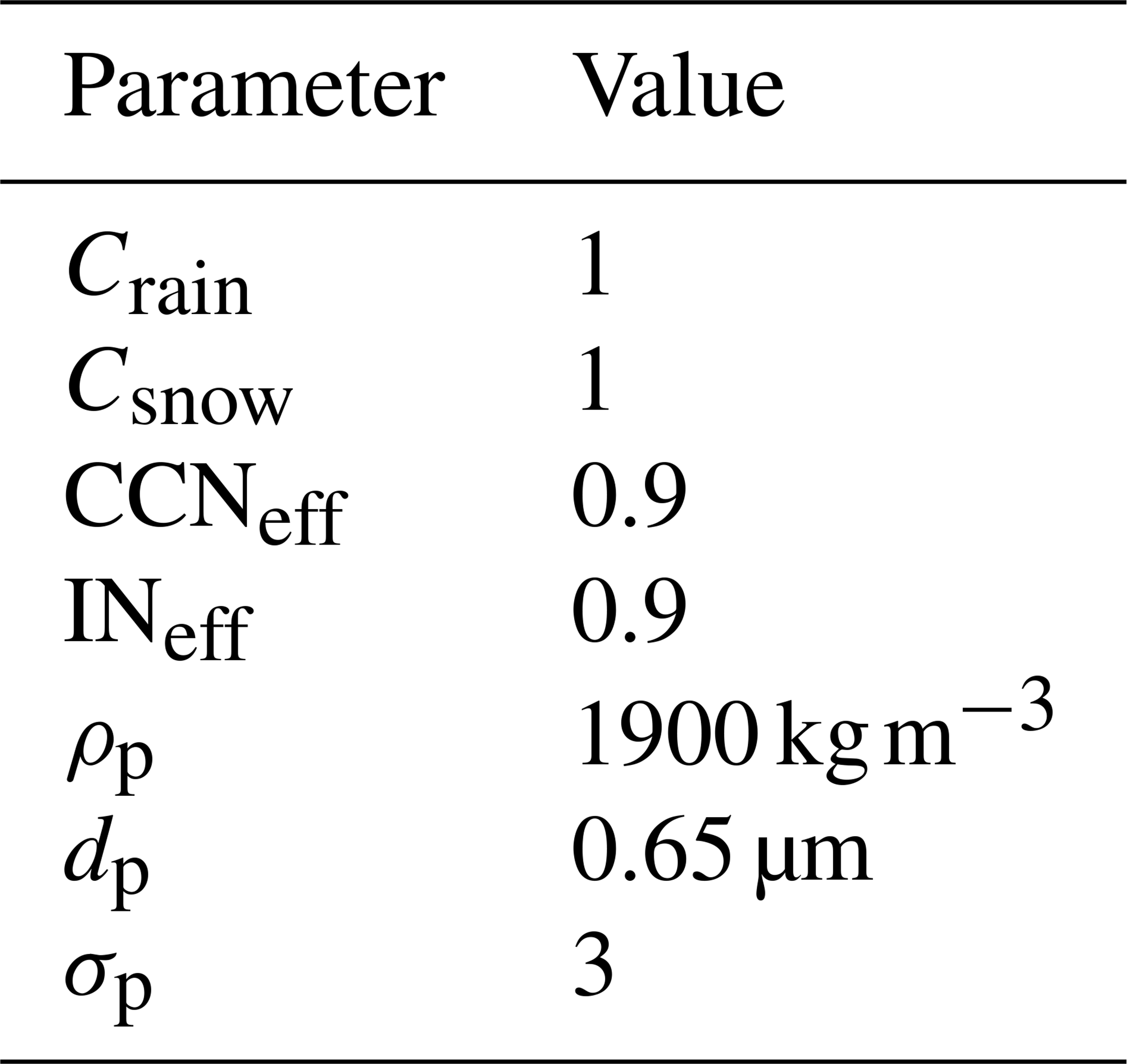
2.7 Translation to FLEXPART parameters

In order for the results of the optimisation method to be usable in future FLEXPART simulations, one has to translate the optimisation parameters x_i to the physical scavenging coefficients which can be altered in FLEXPART through the input parameters {C_rain, C_rain, CCN_eff, IN_eff} (Table 1). Since the method laid out above is only a post-process approach, it is not necessarily expected to have an exact one-to-one corresponding FLEXPART simulation. Therefore the goal is to find a simulation that matches the optimised concentrations as closely as possible. We propose an ansatz that

$$\begin{array}{}\text{(16)}& {\mathrm{\Lambda }}_i{|}_{\text{optim.}}={\displaystyle \frac{x_i}{x_{i,\mathrm{0}}}}\times {\mathrm{\Lambda }}_i{|}_{\text{initial}}.\end{array}$$

This a priori guess can be motivated as follows. The scaling factors A_i (Eq. 14) are defined analogous to the exponential nature of scavenging (Eq. 2). Therefore an analogy can be drawn between x_iλ_i and Λ_iΔt. By taking the fraction of optimised scavenging over initial scavenging, what remains is Eq. (16).

3 Simulation setup and observational data

This section contains the information (simulation input parameters and data as well as observational data) needed to replicate the results shown in this paper.

3.1 FLEXPART input and meteodata

The numerical weather data used for this study were obtained from the MARS archive of the European Centre for Medium-Range Weather Forecasts (ECMWF). They consist of 6-hourly analysis data complemented by short 3 h forecasts and a spatial resolution of 0.5^∘ covering the Northern Hemisphere. They contain 91 non-uniformly spaced vertical levels, ranging from 10 m to approximately 80 km.

The methods laid out in Sect. 2.3 are applied by using the Lagrangian particle model FLEXPART v10.4. The FLEXPART calculations are performed with 10 million particles over the period from 11 March 2011 at 00:00 UTC to 5 April 2011 at 00:00 UTC. The results are output in 3 h intervals. The ¹³⁷Cs source term for the FDNPP release is taken from Terada et al. (2020) and the ¹³³Xe source term from Stohl et al. (2012). The relevant deposition parameters are shown in Table 1 with their initial values. The mean particle diameter d_p is not the default value, but is instead chosen to be in better agreement with measurements from the aftermath of the FDNPP accident (Kaneyasu et al., 2012; Masson et al., 2013; Miyamoto et al., 2014). Concentration and deposition values are output over a 3 h interval on a 0.5^∘ grid.

3.2 Observational data

Measurements of ¹³⁷Cs and ¹³³Xe air concentrations are provided by the Comprehensive Nuclear-Test-Ban Treaty Organisation (CTBTO). The ¹³⁷Cs data consist of 248 measurements across 20 radionuclide stations of the International Monitoring System (IMS) that measured the highest amount of ¹³⁷Cs over the simulation period (Fig. 1). For the ¹³³Xe comparison 626 measurements were used across the 19 IMS stations with the highest measured concentration for this radionuclide. The IMS stations are implemented as receptors in FLEXPART, which – through the use of a parabolic kernel – give more accurate values compared to a grid output (Stohl et al., 1998). The IMS measurements are daily averaged concentrations for ¹³⁷Cs and daily or twice daily for ¹³³Xe. In order to compare the FLEXPART simulations to the IMS observations, the simulation output is averaged over the integration time of the measurements (i.e. 24 h for ¹³⁷Cs and 24 h or 12 h for ¹³³Xe).

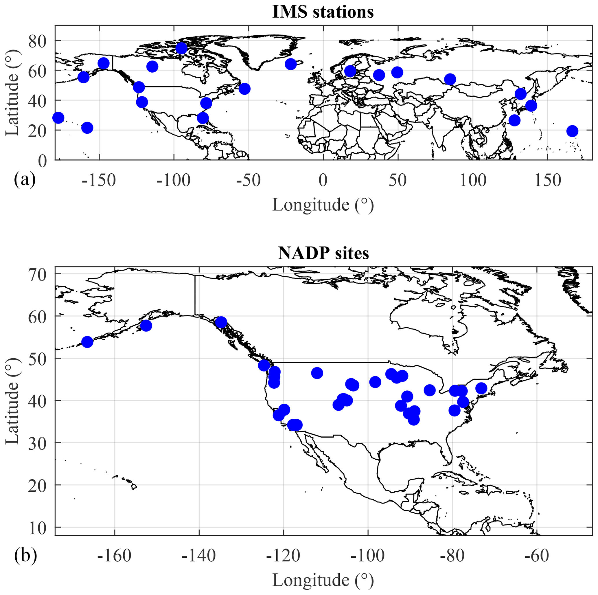
Figure 1 Locations of the measurement stations used in this study. (a) IMS stations. (b) NADP sites.

Furthermore, wet deposition measurements of ¹³⁷Cs from the National Atmospheric Deposition Program (NADP) in the United States are used (Wetherbee et al., 2012). These data were obtained by the use of collectors that open only when it rains, thus minimising the contamination by dry deposition. The dataset consists of measured radioactive samples from 35 NADP sites across the contiguous United States and Alaska (Fig. 1). The deposition data for each site were integrated over a 1- to 2-week period ranging from 8 March to 5 April 2011. Since FLEXPART does not allow the use of receptors for collecting deposition values, the NADP sites are compared to the closest FLEXPART grid points.

4 Results and discussion

In this section we show the results obtained by applying the above method to the Fukushima nuclear accident. First, we show the results of a FLEXPART simulation with initial parameters of Table 1, referred to as the “reference” simulation, in Sect. 4.1. Section 4.2 visualises the results of the individual scavenging contributions. The next section, Sect. 4.3, shows the results of the optimisation scheme. Finally, the results of the translation from optimisation to FLEXPART parameters are shown in Sect. 4.4.

4.1 Reference simulation

In order to assess whether the optimisation scheme provides improved agreement between simulations and observations, a simulation is conducted with deposition parameters of Table 1. This simulation will be used as a reference for the sake of comparing the results of the optimisation scheme. However, of the 20 stations implemented as receptors in FLEXPART, the results of station RN38 located in Takasaki (Gunma), Japan (36.3^∘ N, 139.1^∘ E), were troubling. The station is located only 200 km west of the FDNPP. FLEXPART produced radionuclide concentrations up to 5 orders of magnitude too low compared to observations, thus heavily skewing the resulting statistical analysis. Due to its proximity, it is known that the interior of the building became contaminated and showed incorrect measurements (Stohl et al., 2012). For this reason, the measurements of station RN38 were discarded in the further analysis. We do not take into account any ¹³⁷Cs background, as its contribution is considered negligible, being of the order of 0.1 to 1 µBq m⁻³ (Masson et al., 2015; Biegalski et al., 2001).

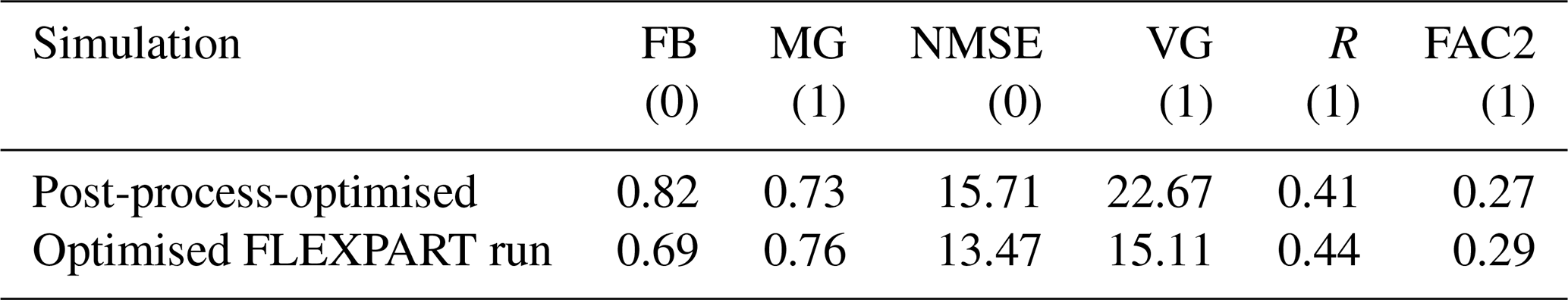
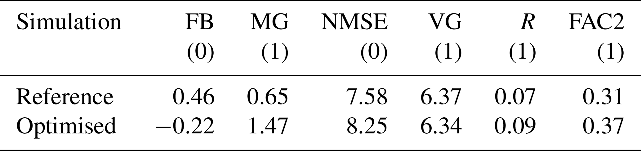
The top row of Fig. 2 shows the simulated air concentrations of ¹³⁷Cs compared to the IMS observations in both a scatter plot form and a histogram. With the initial deposition parameters, the simulation shows an overestimation of the air concentration by around a factor of 5. The performance of the reference simulation is further quantified by several statistical scores shown in Table 2. The metrics chosen are the fractional bias (FB), the geometric mean bias (MG), the normalised mean square error (NMSE), geometric variance, the correlation coefficient (R) and the fraction of predictions within a factor of 2 of observations (FAC2). A perfect model would have scores $\text{MG}=\text{VG}=R=\text{FAC2}=\mathrm{1}$ and $\text{FB}=\text{NMSE}=\mathrm{0}$. The performance of the reference simulation is not particularly satisfying. We identify four potential sources of error that can explain this discrepancy: (i) the wind fields, (ii) the source term, (iii) the precipitation data and (iv) the deposition scheme.

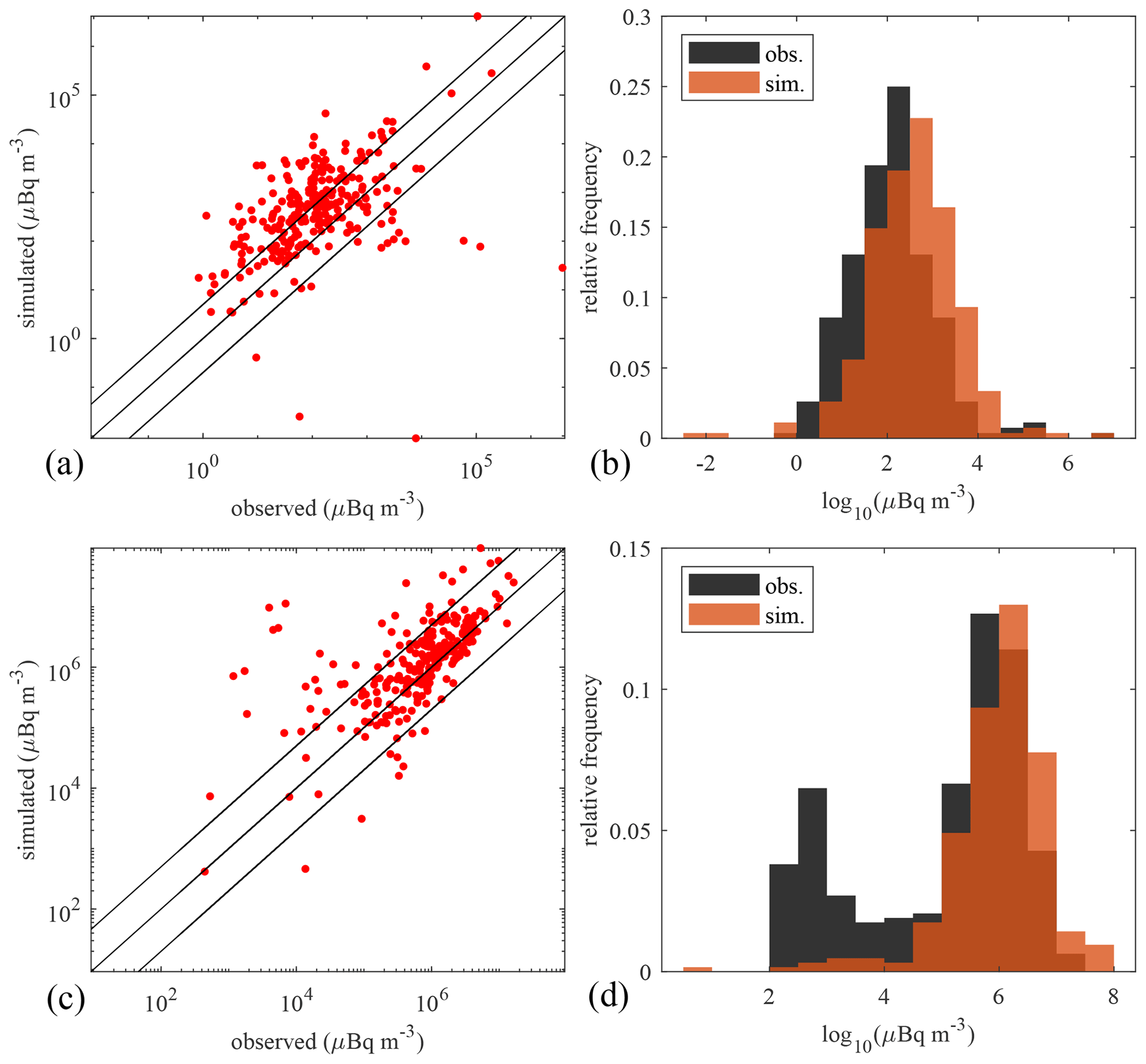
Figure 2 (a, b) ¹³⁷Cs concentrations – reference simulation vs. IMS observations. (c, d) ¹³³Xe air concentrations – simulated vs. IMS observations.

Table 2 Statistical scores of the ¹³⁷Cs simulation with default scavenging parameters in FLEXPART and of the ¹³³Xe simulation. The scores of an ideal model are in parentheses.

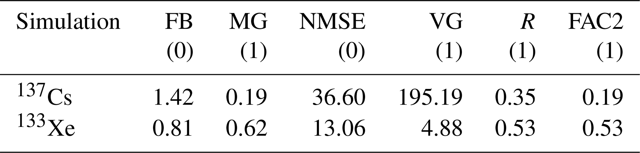
In order to eliminate the possibility that the wind fields cause this discrepancy, we evaluate the transport and dispersion of ¹³³Xe during the FDNPP accident. Xe is a noble gas and is therefore not subject to deposition. The winds are thus what drive its transport and dispersion. The scatter plot and histogram of the simulated Xe air concentrations and corresponding IMS observations are shown in the bottom row of Fig. 2. These show much better agreement between observations and simulations. The observational peak around ∼10³ µBq m⁻³ is likely to originate from regulated emission sources such as medical isotope production facilities, nuclear power plants and research reactors (Gueibe et al., 2017) which were not taken into account in the simulation. Here we are only interested in the Xe originating from the FDNPP accident. Therefore, only the values above 10^4.5 µBq m⁻³ are considered. The statistical scores for this subset of the data are shown in Table 2. The Xe simulation performs much better than the Cs simulation. From this, it can be concluded that the winds are not mainly responsible for the large discrepancy found in the reference ¹³⁷Cs simulations.

No uncertainty range for the FDNPP source term is given by Terada et al. (2020). Looking at other source terms found in the literature, in order to make an uncertainty estimate, suggests that the source term of Terada et al. (2020) is on the lower end in terms of total emitted ¹³⁷Cs. The Terada et al. (2020) source term was recently revised from Katata et al. (2015) and reduced the estimated total amount of emitted ¹³⁷Cs by 29 % from 14 to 10 PBq. This is also a reduction of 73 % compared to one of the earliest source term reconstructions of the FDNPP incident by Stohl et al. (2012), which gave a total emission of 37 PBq, with an uncertainty range of 20–53 PBq. Since FLEXPART is a linear dispersion model – meaning that the air concentrations scale linearly with the source term – an additional reduction of a factor of 5 in the source term would be needed to explain the discrepancy seen in the ¹³⁷Cs FLEXPART simulation. Thus, considering that the Terada et al. (2020) source term already appears on the lower end of available estimated source terms, we consider the source term to be an unlikely main source of the discrepancy.

To tackle a potential flaw in the use of the precipitation data, we also compare the ECMWF precipitation (as obtained through the use of the Flex_extract software; Tipka et al., 2020) to observations by the Global Precipitation Climatology Project (GPCP; Adler et al., 2023, 2018). The GPCP data are based on microwave and infrared satellite measurements and are calibrated with rain gauge observations by the Global Precipitation Climatology Centre (GPCC; Schneider et al., 2011). Figure 3 shows the GPCP and the ECMWF data. The precipitation is integrated over the whole month of April 2011. A good correspondence is seen between the GPCP and the ECMWF data.

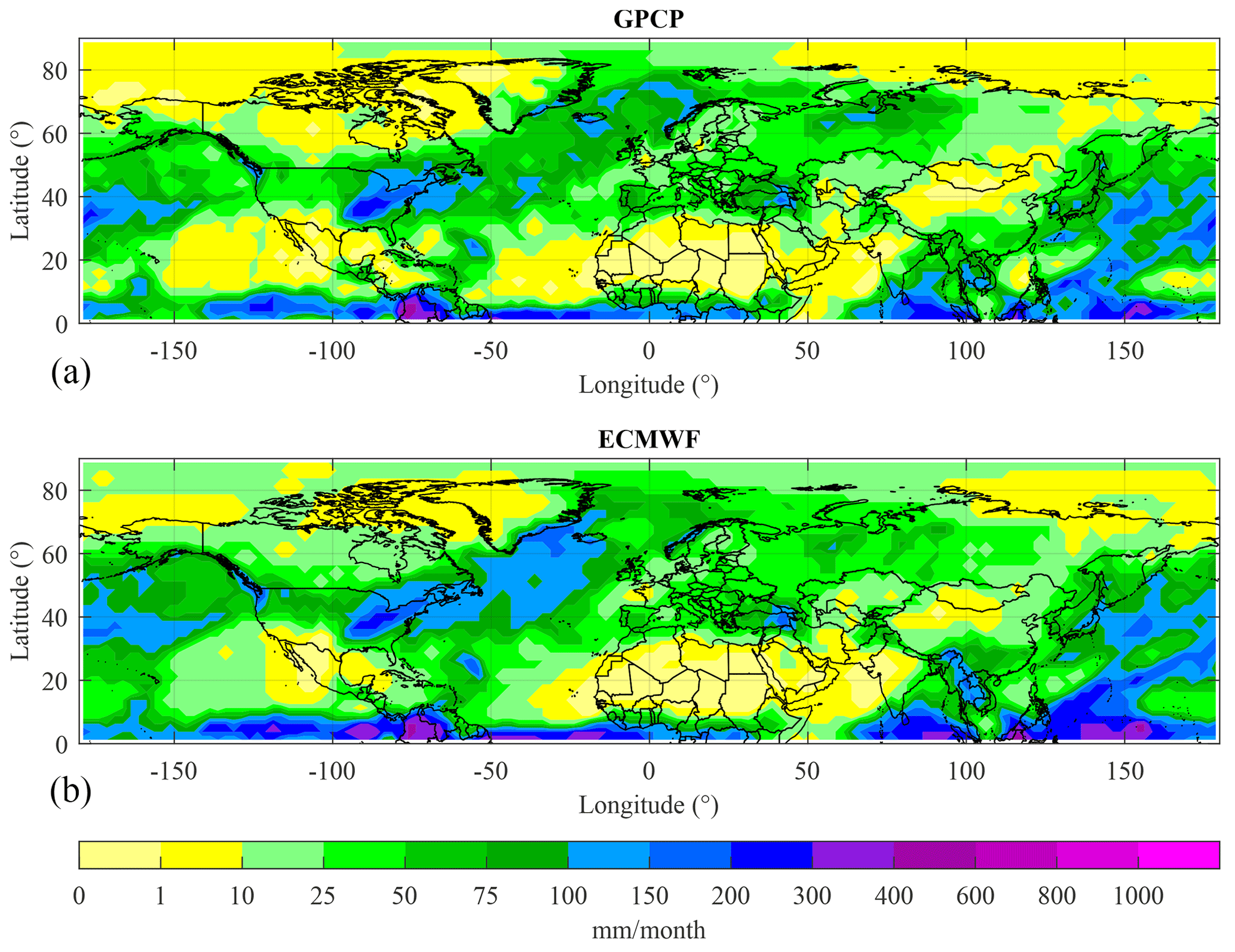
Figure 3 (a) GPCP precipitation data for the month of April 2011. (b) ECMWF integrated precipitation over the month of April 2011.

Given the above validation of the meteorological data and the source term, we conclude that the discrepancy of the reference simulation probably lies in the deposition scheme in FLEXPART. We seek an improvement by finding new, better input parameters to the wet deposition scheme compared to those in Table 1.

The results from Fig. 2 stand in contrast to simulations of the FDNPP accident with FLEXPART v9, such as Stohl et al. (2012), where an underestimation of the air concentrations is found. This can be explained by the fact that the scavenging has generally decreased in FLEXPART v10.4 compared to v9 (Grythe et al., 2017). Grythe et al. (2017) find that the modelled aerosol lifetime of ¹³⁷Cs for the Fukushima case went from 6 d in FLEXPART v9 to 10 d in v10, with no significant bias in modelled versus observed air concentrations of the latter. The observed aerosol lifetime from measurements is closer to 14 d. A longer lifetime is associated with higher air concentrations. Our reference simulation, however, finds an overestimation of the air concentrations for FLEXPART v10. This discrepancy compared to the Grythe et al. (2017) study can potentially be attributed to the fact that Grythe et al. (2017) use multiple particle size bins ranging from mean diameters of 0.4 to 6.2 µm. We have considered a single size bin with a particle diameter of 0.65 µm, as this corresponds more closely to the particle sizes found in measurements (see Sect. 3). Table 3 in Grythe et al. (2017) provides some of their results with the use of single size bins. There it is found that releasing all mass in the size bin of 0.65 µm results in a relative air concentration bias of 11. This is an overestimation, similar to what we found in our reference simulation.

The motivation for our choice of particle diameter is as follows. The change in wet deposition scheme between FLEXPART v9 and v10 suggests that wet deposition is a major contributor to changes in air concentrations for the Fukushima case between the two FLEXPART versions. Therefore we have chosen to focus solely on the wet deposition scheme. Dry deposition is more sensitive to particle size compared to wet deposition, the latter of which is only dependent on particle size in the below-cloud scavenging scheme of FLEXPART. Hence, we did not alter the particle size distribution further.

Stohl et al. (2012) found large model differences between the use of ECMWF and the Global Forecast System (GFS) for the FDNPP case. The influence of the numerical weather data manifests not only as a difference in the spatiotemporal precipitation pattern, but also in the cloud water fields that are used by FLEXPART to quantify below- and in-cloud scavenging. Although the methods presented herein can be used with any numerical weather data, the resulting wet deposition parameters can be specific for said data.

4.2 Scavenging contributions

Step 1 in the methods is to quantify the individual scavenging contributions of the reference simulation (Sect. 2.4). Figure 4 (left panel) shows the scavenging contributions of the reference simulation for the IMS radionuclide station RN71 (Sand Point, Alaska, US; 55.3^∘ N 160.5^∘ W). The horizontal axis starts on 18 March 2011, when the simulated plume first reached the receptor. The vertical axis shows the relative amount of each contribution compared to the concentration c₀ (i.e. the fictitious concentration that would be left over without any scavenging). The values are daily averaged concentrations as calculated by the parabolic kernel method in FLEXPART. The relative sum of all scavenging contributions and remaining air concentration is equal to 1, in accordance with Eq. (10). Figure 4 thus quantitatively shows which part of the concentration has been removed due to the different scavenging processes for the part of the plume that reaches the detector during a given time period.

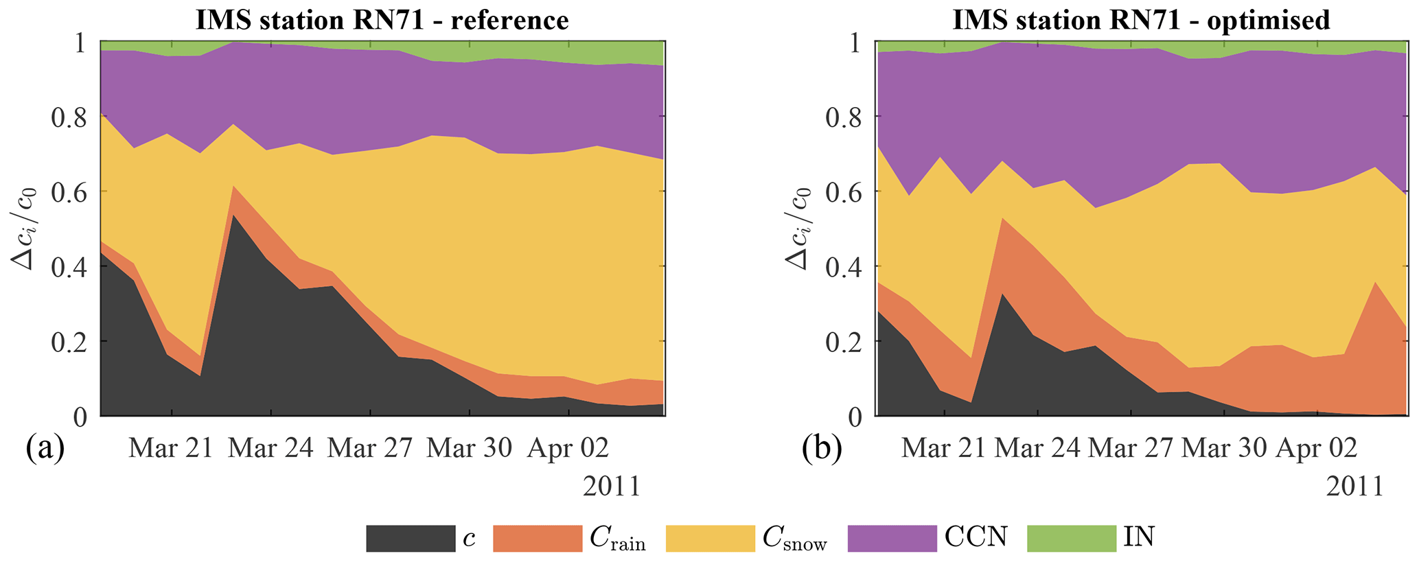
Figure 4 Simulated relative contributions of the different removal processes of ¹³⁷Cs for the RN71 station following the FDNPP accident. (a) Reference simulation. (b) Post-process-optimised concentrations.

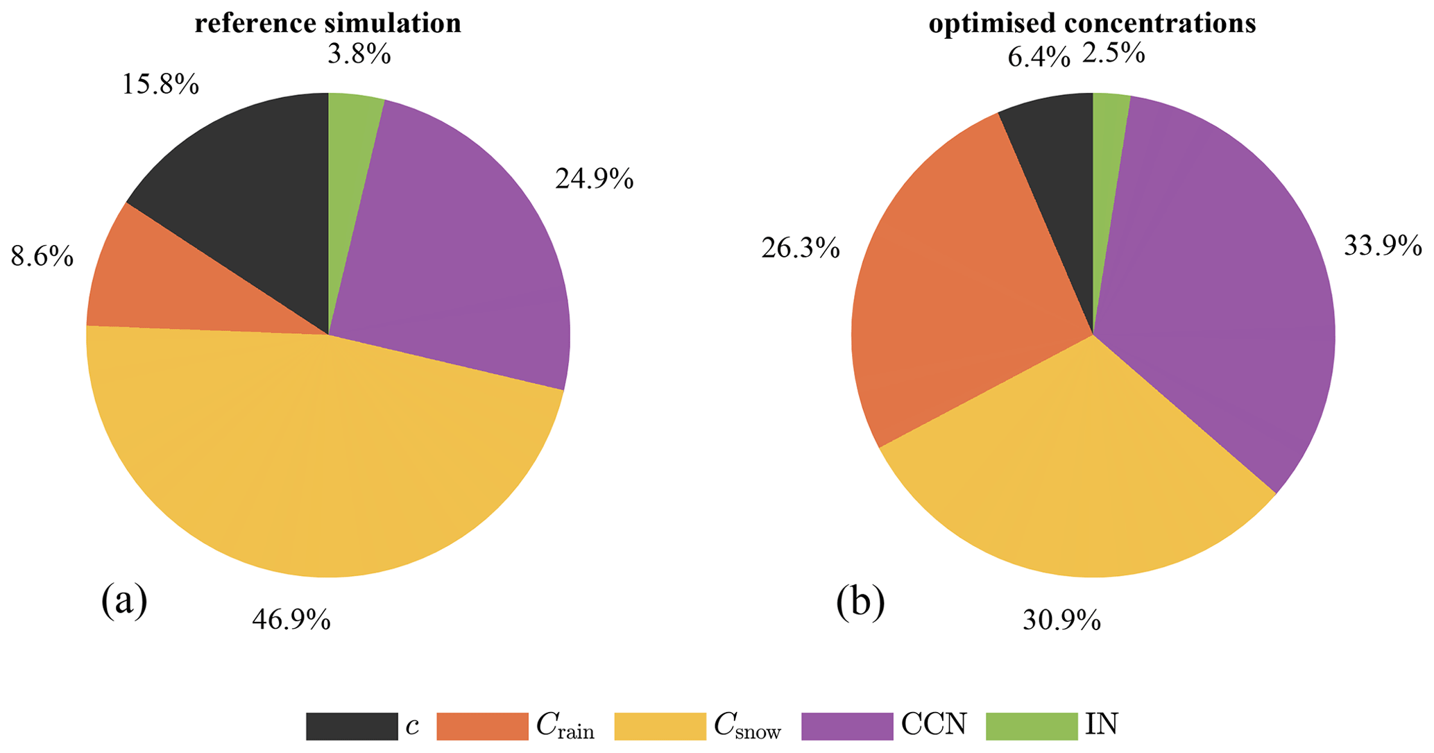
Figure 5 Total simulated contributions of the different removal processes over all stations. (a) Reference simulation. (b) Post-process-optimised concentrations.

Note that the air concentration left over after scavenging (c, black coloured area), as with all quantities on this plot, is relative to c₀. The fictitious concentration c₀ is determined only by the winds and not deposition, much like what would be the case with a noble gas such as xenon. Therefore unlike the temporal variations in c, the variations in the ratio $c/c_{\mathrm{0}}$ are not mediated by the wind fields, but instead solely by spatiotemporal variations of the different removal processes. In other words, the wind field variations are divided out by taking the quantities relative to c₀.

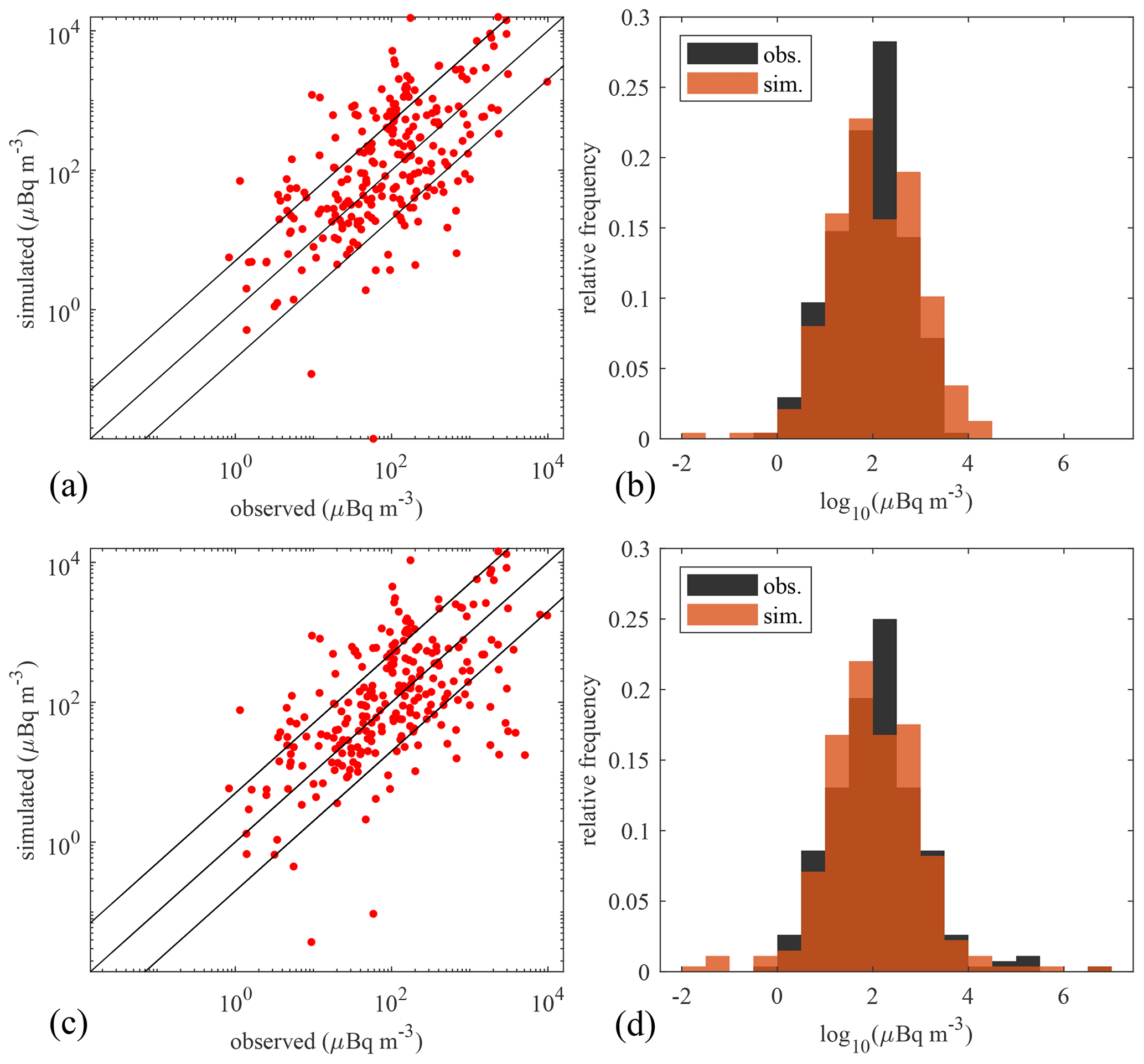
Figure 6 (a, b) Post-process-optimised ¹³⁷Cs concentrations vs. IMS observations. (c, d) ¹³⁷Cs concentrations from the optimised FLEXPART run vs. IMS observations.

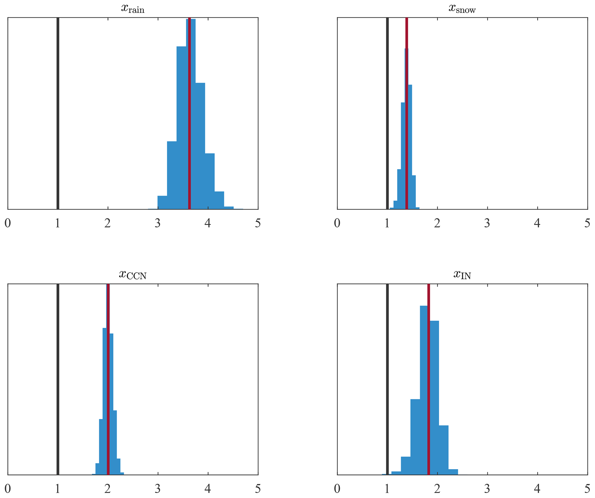
Figure 7 Distribution of the optimisation parameters x_i as a result of 10 000 samples of a random selection of 50 % of the available measurements. The black vertical lines represent the unoptimised default values x_i,0. The red vertical lines denote the values found by using all measurements (Table 4).

An overview of the scavenging processes across all stations is shown in Fig. 5 (left panel). It covers the whole simulation period (11 March–5 April 2011). In total 84 % of the concentration is scavenged and deposited in the reference simulation. 66 % of the wet scavenging occurs below cloud, while 34 % occurs in cloud. The partitioning of below- and in-cloud scavenging found here is in contrast to that of some previous studies (Andronache, 2003; Henzing et al., 2006; Arnold et al., 2015; Grythe et al., 2017; Pisso et al., 2019a), which found that in-cloud scavenging has a greater influence on deposition values than below-cloud scavenging. An explanation for this discrepancy can likely be found in either the use of erroneous methods for calculating the partitioning or in the underestimation of the scavenging coefficients in the other studies. Whereas we extracted the Δc_i values directly during a single simulation, Arnold et al. (2015), Grythe et al. (2017) and Pisso et al. (2019a) performed simulation runs of the FDNPP accident with below- and in-cloud scavenging separately disabled. The latter method, however, is subject to compensation effects. Disabling a scavenging process leaves a higher air concentration for the other scavenging process(es). Indeed, by simply disabling a single scavenging process, more mass is available to the other scavenging processes. This compensation effect is avoided in our method as the scavenging contributions are directly extracted from the simulation through alterations of the FLEXPART source code. The method of Andronache (2003) and Henzing et al. (2006) is based on a theoretical approach to the below-cloud scavenging coefficient: a method which is known to underestimate the scavenging coefficient by 1–2 orders of magnitude (Wang et al., 2010, 2011). Recent measurements have indicated that below-cloud scavenging contributes to the majority of the total wet deposition (Chatterjee et al., 2010; Xu et al., 2017; Ge et al., 2021).

4.3 Optimised concentrations

Quantified in the previous section, the individual removal processes were then scaled and optimised according to Sect. 2.6. The optimisation method is able to reduce the bias compared to the reference simulation, as can be seen in the top row of Fig. 6 and the statistical scores in Table 3. An improvement in all statistical scores is seen.

Table 3 Statistical scores of the post-process-optimised ¹³⁷Cs concentrations and of the ¹³⁷Cs concentrations resulting from a FLEXPART simulation with the use of the optimised scavenging parameters in Table 5. The scores of an ideal model are in parentheses.

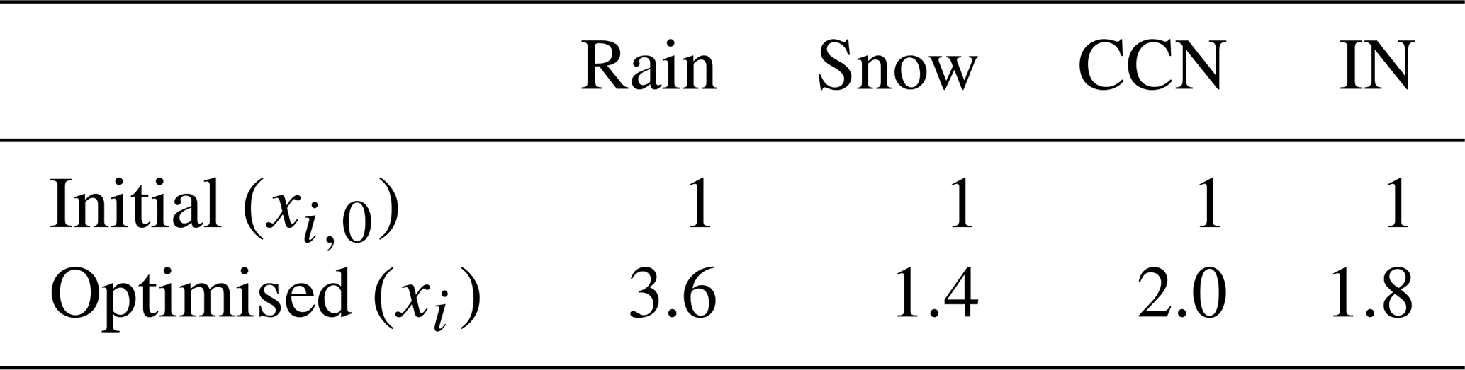
The optimisation algorithm found this best fit with the x_i values (Eq. 14) shown in Table 4. All optimisation parameters have increased, suggesting that the efficiency of all four scavenging processes needs increasing. The greatest increase is found for below-cloud scavenging by rain (×3.6). Below-cloud scavenging by snow changed relatively little with a factor of 1.4. In-cloud scavenging by cloud condensation nucleation (CCN) and ice nucleation (IN) are both increased by slightly greater amounts (×2.0 and 1.8, respectively). The optimised scavenging contributions for station RN71 are shown in Fig. 4 (right panel). Figure 5 (right panel) shows the new removal contributions over all stations. We find that the largest contributor to the total wet deposition is still below-cloud scavenging at 63 % compared to 37 % for in-cloud scavenging. Compared to the reference simulations (Fig. 5, left panel), the total concentration reaching the detectors is reduced from 16 % of the concentration c₀ to 6 %. The greatest increases in scavenging are seen in collection by rain (from 9 % to 25 %) and cloud condensation nucleation (from 25 % to 33 %). One may notice that despite the increase in efficiency of collection by snow, the relative contribution thereof has decreased from 47 % to 33 %. This is the aforementioned compensation effect at play. A greater increase in other processes leaves less concentration available for snow collection. This is similar for ice nucleation, whose contribution has actually shrunk from 4 % to 2 % despite the increase in its efficiency.

Table 4 Optimisation parameters (as in Eq. 14) before and after the optimisation process.

To validate the consistency of these results, the optimisation parameters x_i are also calculated for 10 000 samples of a random selection of 50 % of the available measurements and subsequently applied to the remaining 50 % of measurements. The distributions of the optimisation parameters are shown in Fig. 7. All parameters differ significantly from the default value of 1. The relative standard deviations of the optimisation parameters for rain, snow and CCN scavenging are 6.8 %, 6.1 % and 4.6 %, respectively. Scavenging by ice nucleation (IN) shows a slightly larger relative deviation of 11 %. The statistical scores that result from applying these optimised parameters to the rest of the measurements show a significant improvement over the reference simulation for almost all samples, as can be seen in Fig. 8. A slightly peculiar result is seen for the Pearson correlation coefficient (R), which shows bimodal behaviour. This is likely the result of this score being dominated by larger values since the concentrations span multiple orders of magnitude. Depending on whether the largest detections are selected in the random samples, a different correlation is found.

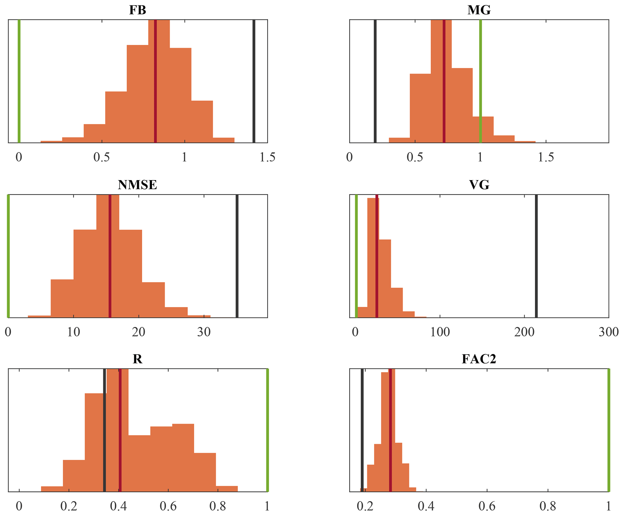
Figure 8 Distribution of the statistical scores as a result of optimising 10 000 samples of a random selection of 50 % of the available measurements and applying the optimised parameters to the rest of the data. The black vertical lines represent the values of the reference simulation (Table 2). The green vertical lines represent the score of a perfect model. The red vertical lines denote the values found by using all measurements (Table 3).

4.4 Translation to scavenging coefficients

The new FLEXPART input parameters, according to Eq. (16), are shown in Table 5. One may notice that according to the optimisation process, the efficiencies of in-cloud nucleation are greater than 1, which is a challenge to interpret physically. If a maximum possible efficiency of 1 is assumed, then larger values of x_i can be interpreted to actually probe other factors in Eq. (5), such as the cloud water replenishment factor i_cr. Since the value of i_cr is not an input parameter to FLEXPART, but is instead defined in the source code, one can still use the optimised values of CCN_eff and IN_eff as input parameters to obtain the result of increased Λ for these processes, albeit with the caveat that one should be mindful with the physical interpretation.

Table 5 Optimised ¹³⁷Cs wet deposition input parameters for FLEXPART v10.4 for the FDNPP accident, as obtained through Eq. (16).

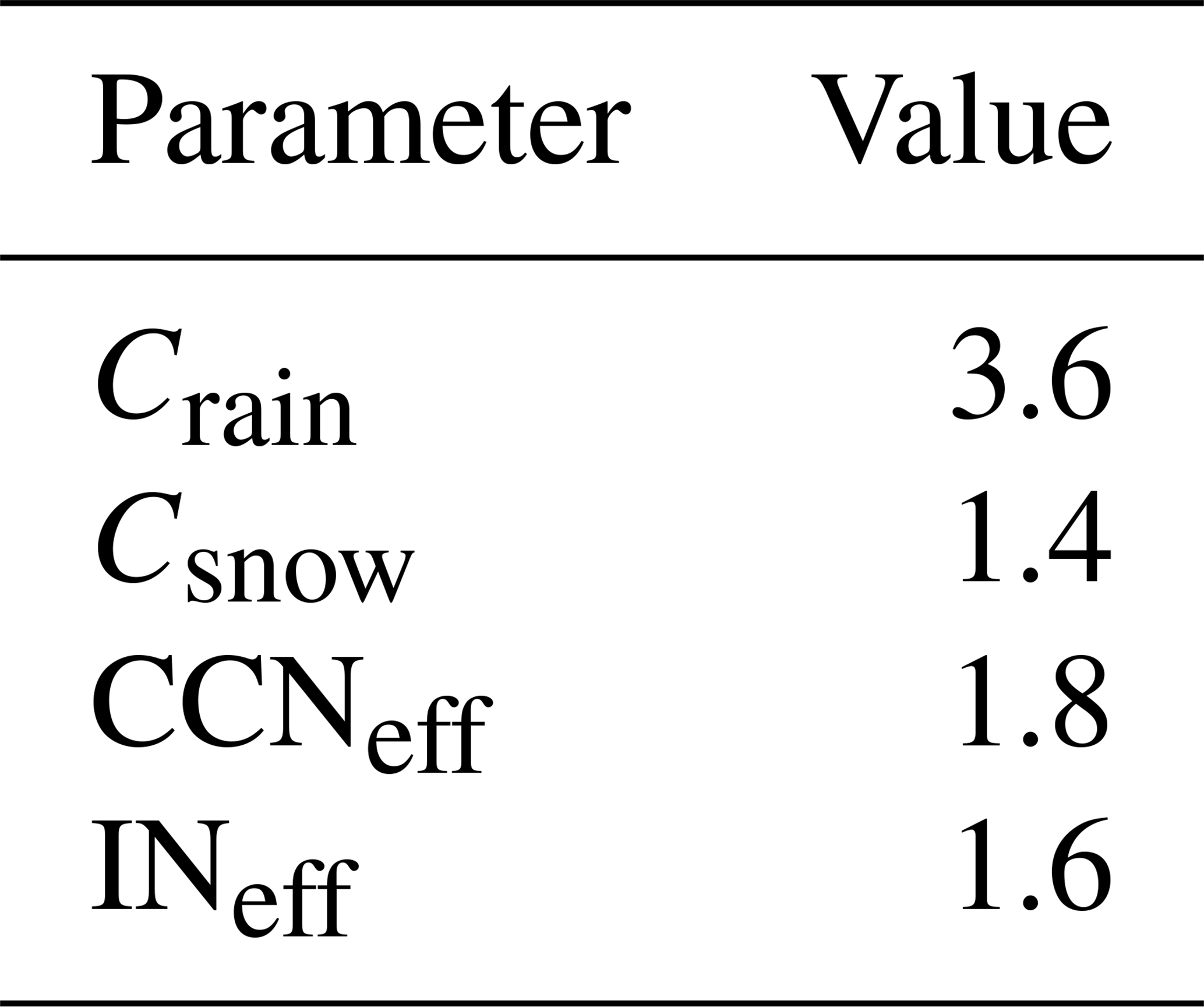
Table 6 Statistical scores of the ¹³⁷Cs deposition values obtained in the reference simulation and in the optimised simulation. The scores of an ideal model are in parentheses.

Using the optimised input parameters from Table 5 in a new FLEXPART simulation leads to the ¹³⁷Cs concentrations shown in the bottom row of Fig. 6. With the ansatz of Eq. (16), results are already obtained that are close to the post-process-optimised concentrations (top row of Fig. 6). A comparison of the new scores in Table 3 with the post-process optimisation even shows a quantitative improvement for all statistical scores.

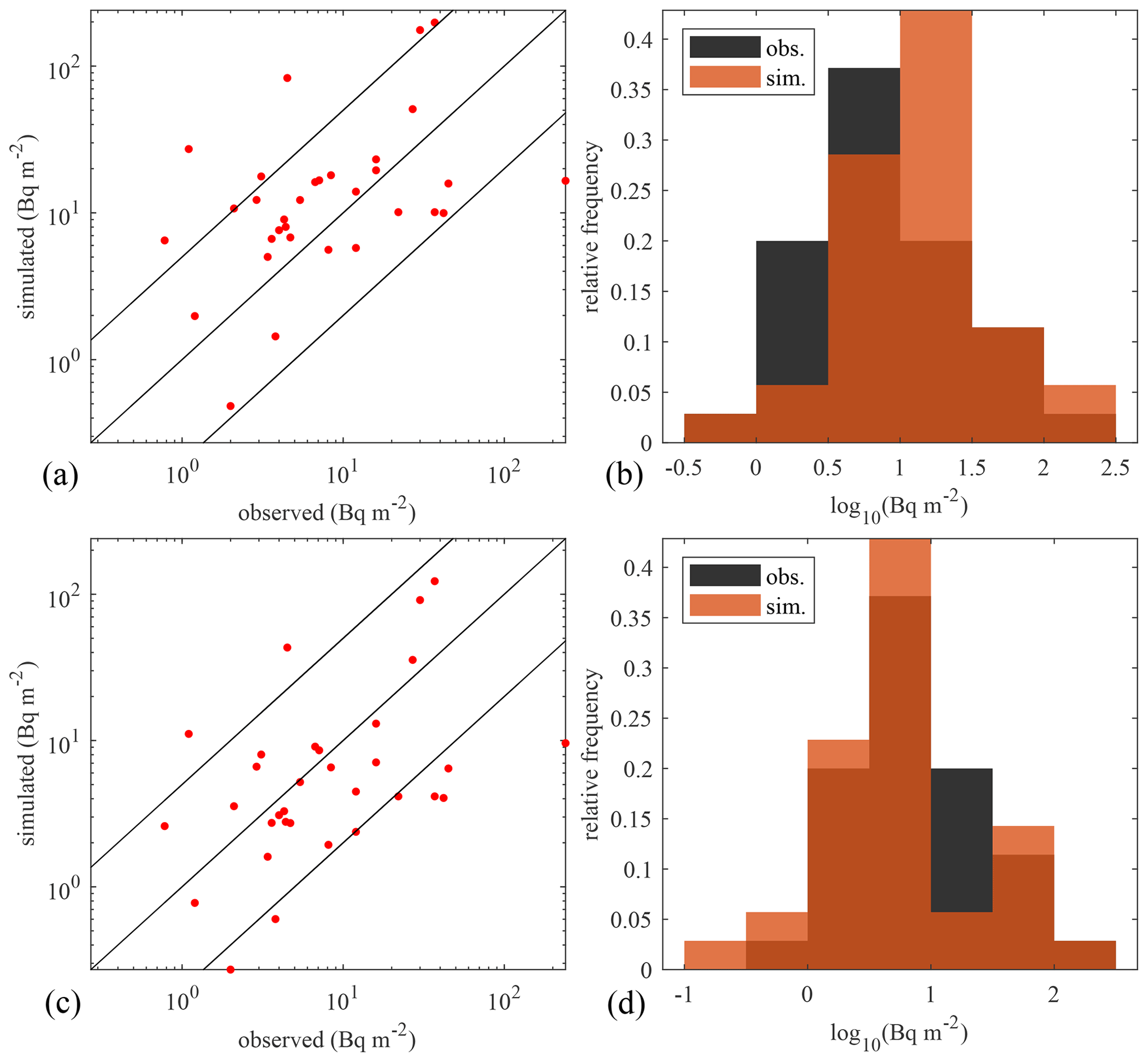
Figure 9 (a, b) Wet deposition of ¹³⁷Cs – reference simulation vs. NADP observations. (c, d) Wet deposition of ¹³⁷Cs – optimised simulation vs. NADP observations.

Note that the optimised FLEXPART parameters of Table 5 are likely to depend on the numerical weather model used, as it can account for model-specific biases in the precipitation and 3D cloud water fields.

4.5 Independent verification with wet deposition measurements

Finally, we present an independent check of the results by looking at the wet deposition measurements from NADP. The deposition values of the reference simulation and NADP observations are shown in the top row of Fig. 9, and the corresponding scores are in Table 6. The reference FLEXPART predictions are a better match with the observations in this case compared to the air concentrations as seen previously. Still, a slight bias for overprediction is seen. The optimised FLEXPART simulation is shown in the bottom rows of Fig. 9 and Table 6. A marginal improvement is seen in FB, VG, R and FAC2 and a slight deterioration of MG and NMSE. Overall, we can say that the optimisation process has neither significantly improved nor worsened the deposition results. This is despite the overprediction found for the air concentrations in the reference simulation. This is the result of two competing effects: an increase in deposition reduces air concentration, but also a higher air concentration increases scavenging and thus deposition. In the deposition results of the reference simulations these two effects almost cancel out.

5 Conclusions

Wet deposition plays a crucial role in many atmospheric aspects, such as the transport and dispersion of airborne radionuclides. Simulating wet deposition in atmospheric transport models, however, remains a challenge. Therefore we have developed a post-processing scheme to optimise the wet scavenging rate in ATMs. This method was applied to a case study of aerosol-attached ¹³⁷Cs following the Fukushima nuclear accident, with the use of the atmospheric transport model FLEXPART. In order to utilise the new optimisation scheme, we accurately determined the partitioning of the scavenging processes as calculated by FLEXPART: (1) below-cloud scavenging by rain, (2) below-cloud scavenging by snow, (3) in-cloud scavenging by cloud condensation nucleation and (4) in-cloud scavenging by ice nucleation. We found that the majority of radionuclides that contribute to ground station measurements are scavenged below cloud. The optimisation scheme is able to reduce the originally overpredicted air concentrations of ¹³⁷Cs from an average factor of 5 to a factor of 2. A proposal is made to translate the post-process optimisation results to the physical scavenging coefficients Λ_i of the different processes. Using these Λ_i values, a FLEXPART simulation could be performed which closely matched the post-process-optimised concentrations. The deposition results of this optimised simulation were compared with measurements made in the US (as an independent check) and show neither a significant improvement nor worsening of the already reasonable prior agreement.

We hypothesise that, although applied to the Fukushima nuclear accident, the optimised scavenging coefficients will be valid more generally under similar conditions using the same numerical weather prediction model (ECMWF). Furthermore, the proposed methods herein could be applied to any ATM other than FLEXPART, even with different scavenging processes modelled. In general, the optimisation scheme will result in a scaling factor of the scavenging coefficient for each scavenging process. In this way, one can circumvent the need to explore the parameter space of scavenging rates with many separate ATM simulations.