Rainbows and climate change: a tutorial on climate model diagnostics and parameterization

Earth system models (ESMs) must represent processes below the grid scale of a model using representations (parameterizations) of physical and chemical processes. As a tutorial exercise to understand diagnostics and parameterization, this work presents a representation of rainbows for an ESM: the Community Earth System Model version 2 (CESM2). Using the “state” of the model, basic physical laws, and some assumptions, we generate a representation of this unique optical phenomenon as a diagnostic output. Rainbow occurrence and its possible changes are related to cloud occurrence and rain formation, which are critical uncertainties for climate change prediction. The work highlights issues which are typical of many diagnostic parameterizations such as assumptions, uncertain parameters, and the difficulty of evaluation against uncertain observations. Results agree qualitatively with limited available global “observations” of rainbows. Rainbows are seen in expected locations in the subtropics over the ocean where broken clouds and frequent precipitation occur. The diurnal peak is in the morning over ocean and in the evening over land. The representation of rainbows is found to be quantitatively sensitive to the assumed amount of cloudiness and the amount of stratiform rain. Rainbows are projected to have decreased, mostly in the Northern Hemisphere, due to aerosol pollution effects increasing cloud coverage since 1850. In the future, continued climate change is projected to decrease cloud cover, associated with a positive cloud feedback. As a result the rainbow diagnostic projects that rainbows will increase in the future, with the largest changes at midlatitudes. The diagnostic may be useful for assessing cloud parameterizations and is an exercise in how to build and test parameterizations of atmospheric phenomena.

1 Introduction

Parameterizations are simplified representations of natural phenomena used in many models, from weather prediction to climate or Earth system models (ESMs). These simplified representations can be diagnostics (not affecting the model evolution) or prognostic (changing model evolution). A major source of uncertainty in models is representing critical Earth system processes at the right scale (Hourdin et al., 2016). This work describes the representation of rainbows in an ESM.

Rainbows may seem trivial, but the basic conditions for a rainbow are particular relationships between clouds, rain, and sunlight. Clouds (through cloud feedbacks) are the major uncertainty for climate feedbacks (Sherwood et al., 2020), and rain formation is critical for severe weather as well as understanding cloud adjustments to aerosols that modulate climate forcing (Bellouin et al., 2020). Ensuring that models simulate the right frequency and fraction, location, and timing of clouds and rain is not trivial and may be a useful integrated metric of the relationships in a model that may in fact be important for climate. Carlson et al. (2022) argue that rainbows also provide “cultural ecosystem services” (people like looking at them).

One of the motivations for diagnosing rainbows is that a rainbow is an integrated metric of the representation of the diurnal cycle of clouds and rain in a general circulation model (GCM). GCMs have long-standing biases in their representation of the diurnal cycle of precipitation, especially over land (e.g., Bogenschutz et al., 2018). This is driven largely by biases in the representation of deep convective systems (e.g., Xie et al., 2019). The expected diurnal cycle of rain is a strong diurnal cycle over land with afternoon and evening peaks, as well as a weaker diurnal cycle over ocean with a peak in early morning (Nesbitt and Zipser, 2003).

Extensive observation networks exist for clouds and rain from the surface and from space, ranging from rain gauges to surface radar, to satellites. Often the presence of rain is hard to detect, either because it does not hit the ground or it may be too light (or in too small a region) to see from space. Rainbows can be a stark visual identification of rain that other measurements miss.

Rainbows are also a tutorial exercise for those learning how to use and develop diagnostics or parameterizations for atmospheric models from large eddy simulation models, to mesoscale models, to ESMs. The issues in representing rainbows are similar to other diagnostic parameterizations such as radar reflectivity (e.g., Fielding and Janisková, 2020) and prognostic representations of sub-grid variability in cloud cover (e.g., Tompkins, 2002), which must take a large-scale estimate of the physical state and determine smaller-scale processes and phenomena.

A rainbow diagnostic enables a unique analysis of the fidelity of model-simulated phenomena to observations, as well as projections of how rainbows may change in the future and why. The reasons can be related back to mechanisms of climate change.

Rainbows require applying basic physical laws to the state of the model, using some absolute quantities and some assumptions, to generate a diagnostic for when and where rainbows would be visible in a model. A rainbow diagnostic raises many general problems with parameterizations (Hourdin et al., 2016), including the assumptions that are made, the difficulty of determining the validity at the right scale, and how to properly evaluate sub-grid-scale processes in physical models at any scale.

We start with a basic review of the essential physics of rainbows, previous scientific work on rainbows, and a description of the model to be used in Sect. 2. We then detail the implementation of the physics in the model in Sect. 3 and Appendix A. The representation of rainbows is diagnostic (it does not effect model evolution), but we will refer to the representation as a “parameterization” or “diagnostic” interchangeably. Section 4 contains a sensitivity analysis of the method and then an overall evaluation of the representation based on current knowledge and available observations. We also look at what the rainbow diagnostic can say about the impact of historical and future climate changes on rainbows. Section 5 discusses critical uncertainties in the parameterization, as well as limits of the approach with respect to the limits of the parameterization. Section 6 summarizes the key findings and provides some overarching thoughts on how this development is relevant for many other more topical and “important” representations in climate models.

2 Methodology

Rainbows are an optical phenomenon. Businger (2021) and Haußmann (2016) both provide reviews of the basic physics, building on work by Nussenzveig (1977). Haußmann (2016) discusses some of the unique physics and optics, and Businger (2021) also discusses the larger social context of rainbows with a focus on Hawaii. The scientific basis for rainbows is often attributed to Descartes (1998), as discussed in Werrett (2001). In addition, Diderot's Encyclopedia (Diderot and d'Alembert, 1751) lists an extensive entry for “arc-en-ciel”, with earlier (and later) experiments discussed.

Figure 1 Schematic of rainbow optics. (a) Refraction of a water drop and the size of a rainbow for (b) low sun angles and (c) high sun angles. Similar to Businger (2021), Figs. 3 and 5.

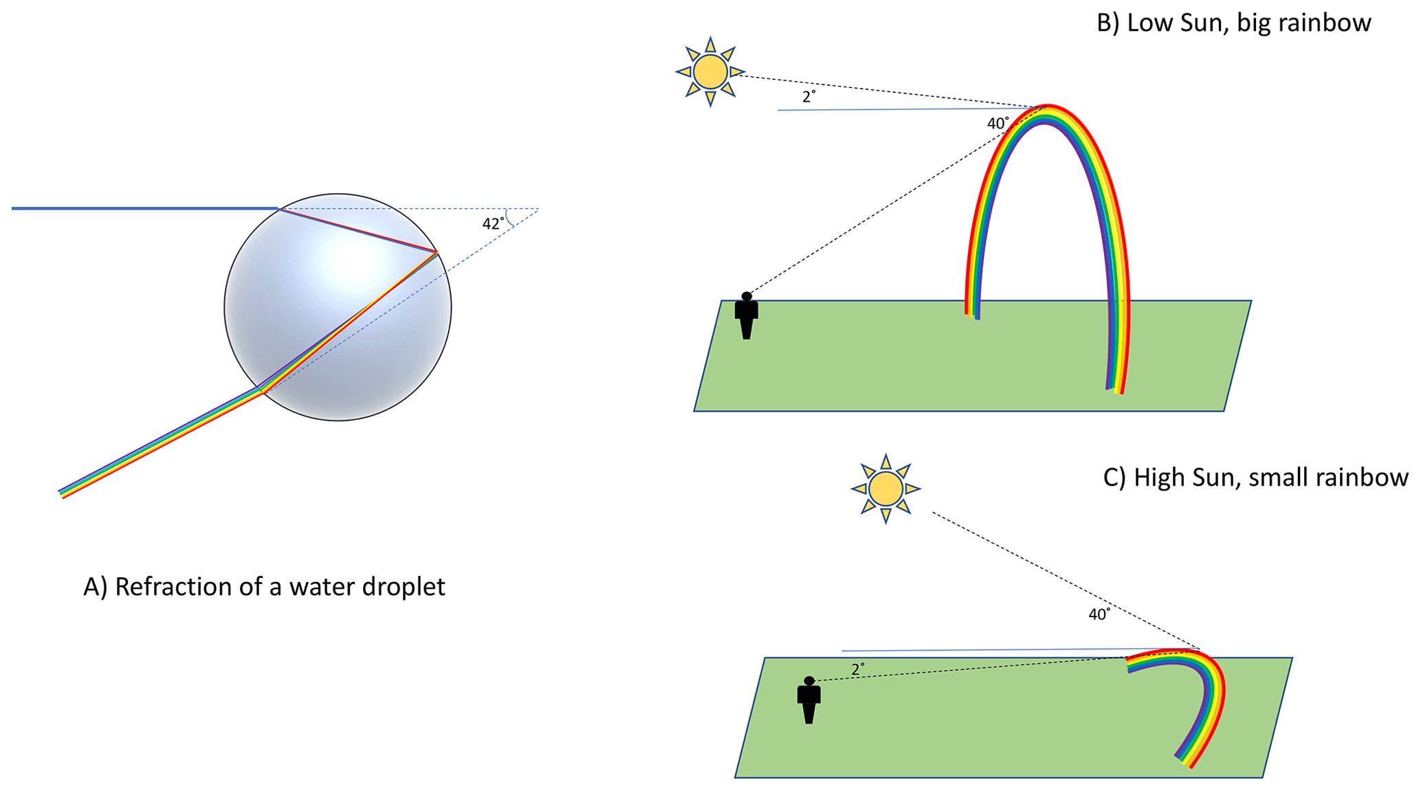
Rainbows occur due to the refraction of light by a raindrop, which separates the colors. Figure 1a illustrates a schematic picture of refraction. Light passes through a raindrop and is scattered back to the observer following a fixed refraction angle of 42^∘. This requires a geometry wherein the light source is behind the observer facing the direction of the raindrop. The light source is usually the sun, which is what we will assume for this exercise, though “moonbows” are also possible. Because of the refraction angle, a rainbow cannot be seen if the sun is higher than 42^∘ from the horizon. Figure 1b and c illustrate that the size of a rainbow in the sky is inversely related to the height of the sun: a maximum (42^∘ arc) when the sun is on the horizon and disappearing when the sun is > 42^∘ above it. Figure 1b shows a large rainbow with a sun angle of 2^∘ above the horizon (low sun), corresponding to a solar zenith angle from the zenith straight above of 88^∘. Figure 1c shows a small rainbow with a sun angle of 40^∘ above the horizon (solar zenith angle of 50^∘).

Businger (2021) and Haußmann (2016) provide many more details on the physics of rainbows, including double (secondary) rainbows (refraction twice within a raindrop) and many other interesting optical properties. For this first attempt, we confine ourselves to the single “primary” rainbow. Quantitative observations of rainbows are few and far between, as befits their status as an optical curiosity and not much more. However, Carlson et al. (2022) recently mined social media posts for rainbows and then used statistical methods to extrapolate to an atlas for “rainbow days” that can be used for comparison. We will return to the potential for rainbow observations in Sect. 5.

3 Implementation

Here we describe the modeling tool we will be using and then present a detailed description of how the representation of rainbows is constructed. Appendix A provides a more detailed description with a specific example as well as discussion of the issues involved in a generalized way to show how just about all representations of physical processes in large-scale models face similar issues.

3.1 Model description

The model we use is a state-of-the-art Earth system model, the Community Earth System Model version 2 (CESM2) (Danabasoglu et al., 2020). The atmospheric component is the Community Atmosphere Model version 6 (CAM6) (Gettelman et al., 2019b), a GCM with ∼ 100 km horizontal and 500 m–1 km vertical resolution with 32 levels up to a top at 3 hPa. The model has a hydrostatic dynamical core on a Cartesian (latitude–longitude) grid and has a physical parameterization time step of 30 min. Liquid cloud occurrence is estimated using the Cloud Layers Unified By Binormals (CLUBB) turbulence scheme (Golaz et al., 2002), implemented in CAM6 by Bogenschutz et al. (2013). This takes the humidity and dynamics of the atmosphere and calculates small-scale turbulence. Turbulence in conjunction with humidity determines the presence of clouds and how much cloud water exists. Ice clouds are treated as described by Gettelman et al. (2010), which allows for ice supersaturation (humidity higher than ice formation) before ice clouds will form, as observed in the atmosphere. Cloud microphysics and precipitation formation are described by Gettelman et al. (2015b) and use a bulk, two-moment representation of hydrometeors with prognostic two-moment rain and snow. This takes the information from CLUBB on clouds and turbulence and determines how many cloud drops exist and how they will interact, grow or evaporate, and/or precipitate for both liquid and ice. Radiative transfer uses the Rapid Radiative Transfer Model for GCMs (RRTMG), described by Iacono et al. (2000). RRTG determines how sunlight and radiant energy from the Earth are scattered and absorbed based on the information about clouds and the heating or cooling that occurs.

The formulation of CAM6 implies important approximations we must consider when trying to represent rainbows. This is a strange and silent world (a hydrostatic model has no sound waves), but it does provide a basis for representing rainbows. The radiative transfer is plane-parallel with angular scattering, but the sun does not actually have a direction or location in the sky. We can calculate a solar zenith angle (SZA or θ_z, the angle from straight up) based on location and time, and the solar radiation has the correct intensity and appropriate scattering but not a specific direction. The sky is still blue because of this scattering. Clouds are divided into large-scale “stratiform” clouds and deep convective clouds. Stratiform clouds are cubic volumes that fill a horizontal part of a grid volume at its full depth and randomly arrange themselves every 30 min. Stratiform clouds have a distribution of cloud particle sizes and a distribution of liquid and ice water mass, but not for the purposes of radiation (they are uniformly gray). Stratiform clouds keep their shape but evolve every 15 min as water condenses, and they produce precipitation. Deep convective motions (“thunderstorms”) are basically small columns that move water up and down with simple microphysics that condense water, detrain it out the top, and precipitate it out the bottom. They disappear and re-appear again at each time step. This is the world in which diagnostic rainbows are defined.

Table 1 Rainbow parameterization parameter values.

3.2 Assembling a rainbow

Rainbows need sun with a given angle and rain present at the same time. So to assemble rainbows we will step through a series of approximations. First, what are we trying to simulate? Since a rainbow needs to be seen to be observed, we are really looking at the “potential” for rainbows given that an observer is present. We do not incorporate the presence of an observer as Carlson et al. (2022) did for rainbow “hot spots”. This does make rainbows different than physical or conservative quantities (such as rain mass). What we are really looking at is the potential based on relationships between quantities, and it is essentially the maximum likelihood: it is possible to see a rainbow under the given conditions if an observer were present in the right place in a grid volume at a given time. We will estimate the frequency of time that a rainbow might be observed in a given volume and the fractional coverage of that rainbow. Next, we assume that in a 100 km horizontal grid box that all rain and rainbows occur in the same grid box. This assumption introduces some important limits on the diagnostic. Like many other “column physics” parameterizations, we assume that we only need worry about the atmospheric state in a single column, not adjacent volumes. This means our diagnostic will break down at a scale in which the rain is not in the same grid box as the rainbow and the observer. A rough estimate of such a scale is about 5–10 km. This comes from assuming a rainbow is near the surface with rain (say 2 km or below) and that the low sun angle limits the distance. A 2 km high rainbow 21^∘ above the horizon (half the maximum) would be 5.3 km away ($\mathrm{2}\mathrm{km}/\text{tan}\left(\mathrm{21}{}^{\circ }\right)$). Smaller rainbows could be further and larger ones closer. At finer scales the parameterization would require some adjustment and communication across columns, which we will discuss at the end. This brings up the important point that even for a very simple parameterization or diagnostic the issues of scale and validity across scales must be considered explicitly.

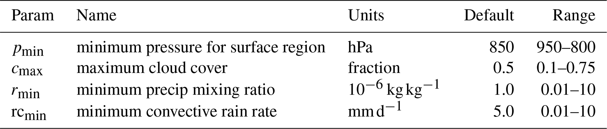
The development and detailed illustrations of each step of the parameterization are described in Appendix A. First, we need to limit the sun angle (θ_z) to within 42^∘ of the horizon. We also need to know how much of the sky a rainbow could cover. This again comes from geometry. A maximum rainbow size will occur when the sun is on the horizon (θ_z = 90^∘), and it will occupy a hemispheric cap of the sky of 42^∘, diminishing to zero when θ_z = 48^∘. Second, there must be some clear sky in a grid box, so we have to set a maximum cloud fraction (c_max) that includes both convective (A_c) and stratiform (A_sr) cloud fraction. Cloud fraction is defined as the maximum overlap of convective and stratiform clouds or max(A_c,A_sr). Third, near the surface of the Earth below some level (which we define with a minimum pressure p_min), there must be some precipitation in the grid box, so we need to set a minimum for the mass of stratiform rain (r_min) and convective rain rate (rc_min) present in a column. Convective precipitation is a surface rain rate (P_c), while stratiform precipitation has mass mixing ratio values (q_rs) throughout the column, so different thresholds are necessary.

Given the four parameters c_max, p_min, r_min, and rc_min, a rainbow exists in a volume when

1. 90^∘ > θ_z > 48^∘,

2. max(A_c,A_sr) < c_max,

3. (P_c>rc_min) or (max(q_rs)>r_min),

where A_c, A_sr, and q_rs are the maximum over model levels from the surface to p_min.

The three criteria above are applied with an appropriate selection of four parameters (p_min, r_min, rc_min, c_max). The parameter values chosen are the “default” values shown in Table 1. Note that these were not just picked randomly but were the result of an initial assessment (sometimes called an expert elucidation or more commonly an educated guess), with subsequent adjustment based on a more rigorous sensitivity analysis (see Sect. 4.2). The results for a particular simulated time (8 January, 12:00 UTC) are illustrated in Fig. 2. Figure 2a indicates where the criteria above are satisfied. For instantaneous data, rainbow frequency is binary (0 or 1) so that the time average is a true frequency of occurrence.

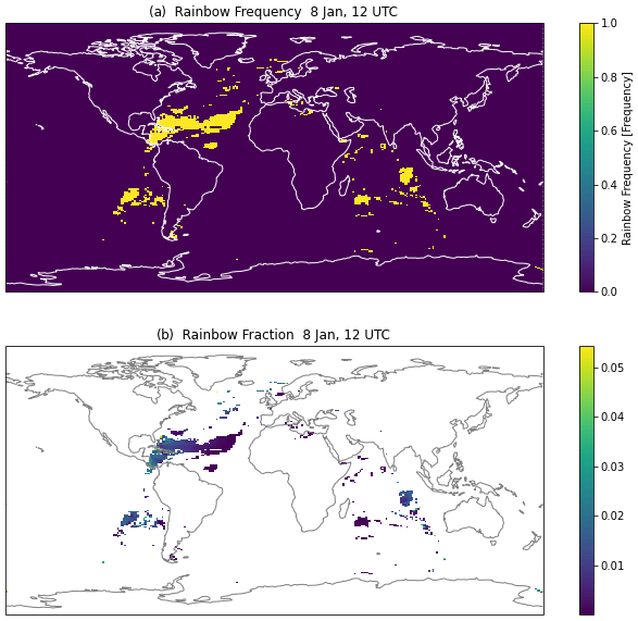
Figure 2 Instantaneous values on 8 January at 12:00 UTC. (a) Rainbow occurrence frequency (1: rainbow). (b) Rainbow fraction of sky covered.

Rainbows of course do not fill the sky, and the probability of seeing a rainbow may be proportional to the area of the sky covered by a rainbow. As indicated in Fig. 1b and c, a rainbow will occupy a hemispheric cap of the sky for a viewer between 0 and 42^∘. As detailed in Appendix A, we define the fractional area of a rainbow Frac_RB as the fraction of the hemisphere for a spherical cap of angle θ_z − 48^∘ multiplied by the rain fraction (A_r):

$$\begin{array}{ll}{\displaystyle }& {\displaystyle }{\mathrm{Frac}}_{\mathrm{RB}}=\mathrm{0}\text{ for }{\mathit{\theta }}_z>\mathrm{48}{}^{\circ },\\ {\displaystyle }& {\displaystyle }{\mathrm{Frac}}_{\mathrm{RB}}=\left(\left(\mathrm{1}-\text{cos}\left({\mathit{\theta }}_z-\mathrm{48}{}^{\circ }\right)\right)/\mathrm{2}\right)\times A_{\mathrm{r}}\text{ for }\mathrm{48}{}^{\circ }>{\mathit{\theta }}_z>\mathrm{90}{}^{\circ },\\ {\displaystyle }& {\displaystyle }{\mathrm{Frac}}_{\mathrm{RB}}=\mathrm{0}\text{ for }{\mathit{\theta }}_z>\mathrm{90}{}^{\circ },\end{array}$$

where the rain fraction A_r is given by the maximum of the stratiform rain fraction (A_sr) and the convective cloud fraction (A_c) in the lower atmospheric layer defined by p_min:

$$A_{\mathrm{r}}=\text{max}(A_{\text{sr}},A_{\mathrm{c}}).$$

Figure 2b illustrates the rainbow fraction (frequency 0 or 1 multiplied by fractional area) for 8 January at 12:00 UTC. Rainbows are found in an arc following the solar zenith angle, with the fraction of the sky covered controlled by the solar angle θ_z (larger with the sun near the horizon) and the fractional occurrence of rain (more rain area results in a larger rainbow).

4 Evaluation and results

The rainbow diagnostic is put into the CAM-specific interface for the cloud microphysics (Gettelman et al., 2015a). Eventually it will be developed as a stand-alone code with an interface for the Common Community Physics Package (CCPP: https://github.com/NCAR/ccpp-scm, last access: 31 July 2023). First we will illustrate basic climatology of where and when rainbows are expected to form. This will include a look at the diurnal cycle of rainbows in different regions, which is important to understand and provides insights on model fidelity. Then we explore the sensitivity of the parameterization to the four parameters. The 4-year-long simulations with climatological boundary conditions for the year 2000 are analyzed for these simulations. To analyze the diurnal cycle, short simulations were conducted with high-frequency output for analysis.

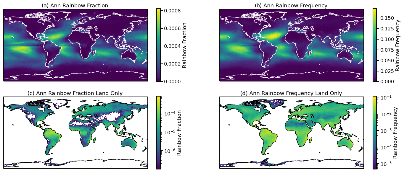
Figure 3 Climatological annual average (mean of 4 years) of diagnosed rainbow (a, c) fraction and (b, d) frequency over all locations (a, b) and just over land (c, d). Note the different scales: there is lower frequency over land.

Quantitative data on rainbow occurrence are scarce. Businger (2021) qualitatively discuss the fact that rainbows are frequent over the Hawaiian islands due to island effects driving precipitation in the subtropical broken-cloud regime. These regions have a diurnal cycle with rainbows morning and evening, with anecdotal and ethnographic evidence: native Hawaiian languages have many words for rainbows. Over midlatitude land, broken clouds associated with thunderstorms in the afternoon and evening also produce rainbows. Similar situations permit rainbows in the evening hours in the summer in monsoon regions. Quantitative climatologies of rainbows to evaluate a parameterization do not exist. Being a ground-based optical phenomenon, rainbows are not observed from space or even from aircraft (other “bows” are seen, e.g., cloud bows, Businger, 2021). Carlson et al. (2022) have attempted to develop a metric for rainbow days based on limited social media observations of rainbows “trained” with precipitation and cloud data to project to other locations. Such data themselves are difficult to evaluate, but in the absence of other data, we can use them for comparison.

4.1 Annual and seasonal means

Figure 3 shows the annual distribution of diagnosed rainbow fraction (sky coverage) and frequency of occurrence (anywhere in the sky) for all points (Fig. 3a and b) and with a different scale to just highlight points over land (Fig. 3c and d). Note that all panels have different scales to highlight key features. The peaks are over the subtropical oceans in regions of stratocumulus (broken) clouds. Peak frequency is in the subtropical Atlantic, with secondary maxima in the central Pacific (near Hawaii) and also south of the Equator.

For clarity, Fig. 3c and d illustrate the same data, but only over land. Note the lower and logarithmic scales. Frequency over land (Fig. 3d) maximizes in the tropics and subtropics of the Southern Hemisphere, with the rainbow fraction (Fig. 3c) being the highest in the tropics. Coastal regions show higher values, including South and Central America and Africa. There are also coastal peaks on the east coast of continents (North America, Asia, and Australia).

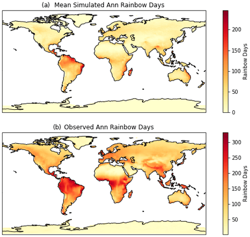
Figure 4 Annual average diagnosed rainbow days over land (see text) for (a) simulations and (b) observations from Carlson et al. (2022).

To attempt to evaluate the parameterization quantitatively, Fig. 4a is a map of rainbow days to compare to Carlson et al. (2022). Rainbow frequency for 4 years is turned into a binary value each day. Any rainbow frequency > 0 means that day is a rainbow day at the given location. The number of rainbow days is calculated for each year, and then an average over 4 years is created. The variability (standard deviation) of rainbow days over each year at any point is about 10 % of the value. The data can then be compared to the dataset from Carlson et al. (2022), derived by learning a relationship between rainbows observed in social media images and precipitation and cloud fraction from reanalysis, illustrated in Fig. 4b. The parameterization locations and magnitudes are highly correlated (0.75) with the dataset machine-learned from observations but are about 50 % lower (the slope of a point-by-point regression line is 0.47). As we will explore, this difference could be “tuned” away if desired. However, the observations are subject to a number of potential biases, so perhaps further exploration of both the simulations and observations is warranted.

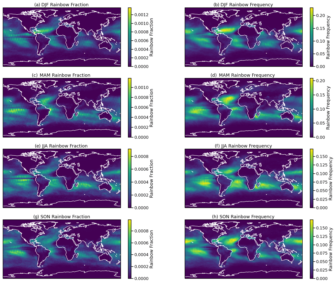
Figure 5 Seasonal average diagnosed rainbow fraction (a, c, e, g) and frequency (b, d, f, h) for different seasons. (a, b) December–February (DJF), (c, d) March–May (MAM), (e, f) June–August (JJA), and (g, h) September–November (SON).

Seasonally (Fig. 5), rainbow frequency is found in the same regions over the ocean, with Southern Hemisphere peaks in subtropical winter (JJA) and Northern Hemisphere peaks in fall (SON) and winter (DJF). The maxima in the subtropics of both hemispheres in winter are due to lower sun angles expanding the times of day when a rainbow can form in these regions, while sufficient liquid precipitation still occurs throughout the year near the surface over the ocean. As noted by Businger (2021), the Hawaiian islands see solar angles that permit rain formation for 6.5 h (58 % of daylight hours) in summer but 8.5 h (78 % of daylight) in winter. Thus over the oceans in both hemispheres, the solar angles seem more important for the seasonal cycle than clouds or rain. Over land, colder temperatures mean more winter precipitation is in the ice phase (snow), and ice does not form rainbows (different refraction patterns). Frequency and fraction track each other in location and magnitude (note the slightly different scales in each season to bring out the different locations). The pronounced banding of fraction (Fig. 5a, c, e, and g) is an artifact of the discrete calculation of solar zenith angle every half-hour time step (with 48 time steps per day).

The seasonal cycle over land (Fig. A5) is different than ocean in many locations. There is little rainbow frequency over Northern Hemisphere land in winter and a peak frequency in spring over Europe and Asia. The tropics have relatively high frequency all year. The southeastern US has moderately high frequency in all seasons but winter. Southern Hemisphere land is generally more subtropically situated and thus has higher frequency in midlatitudes, as well as high frequency in the tropics. Southern Hemisphere arid regions seem to have a higher rainbow frequency and fraction than the Northern Hemisphere. This might be due to dry land masses over the larger continents. More evaluation based on local conditions is warranted. In addition, we can analyze the diurnal cycle of rainbow diagnostics in key regions, including over land.

4.2 Diurnal cycle and sensitivity

The diurnal cycle of clouds and precipitation naturally gives rise to rainbows at different times of the day in different cloud regimes. The rainbow diagnostic can be used to evaluate if the GCM matches observed rainbow timing. We can also use the diurnal cycle to test the sensitivity of the rainbow diagnostic to the choice of each of the four parameters in Table 1 (r_min, rc_min, p_min, c_max). The results in Sect. 4.1 above are default settings. Sensitivity tests are conducted with the standard simulation. We have evaluated sensitivity tests conducted with the climate change scenarios (see Sect. 4.3), and sensitivities for all the parameters are qualitatively the same with only small quantitative differences when altered climate conditions are used.

To analyze the diurnal cycle and explore sensitivities, we archived time-step-level output for 2 months: January and July. We took the model output for all the needed inputs to the rainbow diagnostic and then calculated the rainbow diagnostic directly from those inputs, varying the parameters used. This produces the same result as calculating the diagnostic within the model as it runs. The results are not bit for bit due to slight differences in where the output of the model occurs in the time step loop relative to where the rainbow diagnostic is calculated, but results are qualitatively the same. Rainbow frequency and fraction are generated for a range of each of the four parameters separately in Table 1. To better visualize the sensitivity, monthly averaged diurnal cycles were created in six regions: three for January and three for July. Regions and their locations are listed in Table 2.

Table 2 Regions selected for analysis of rainbow parameterization diurnal cycle sensitivity.

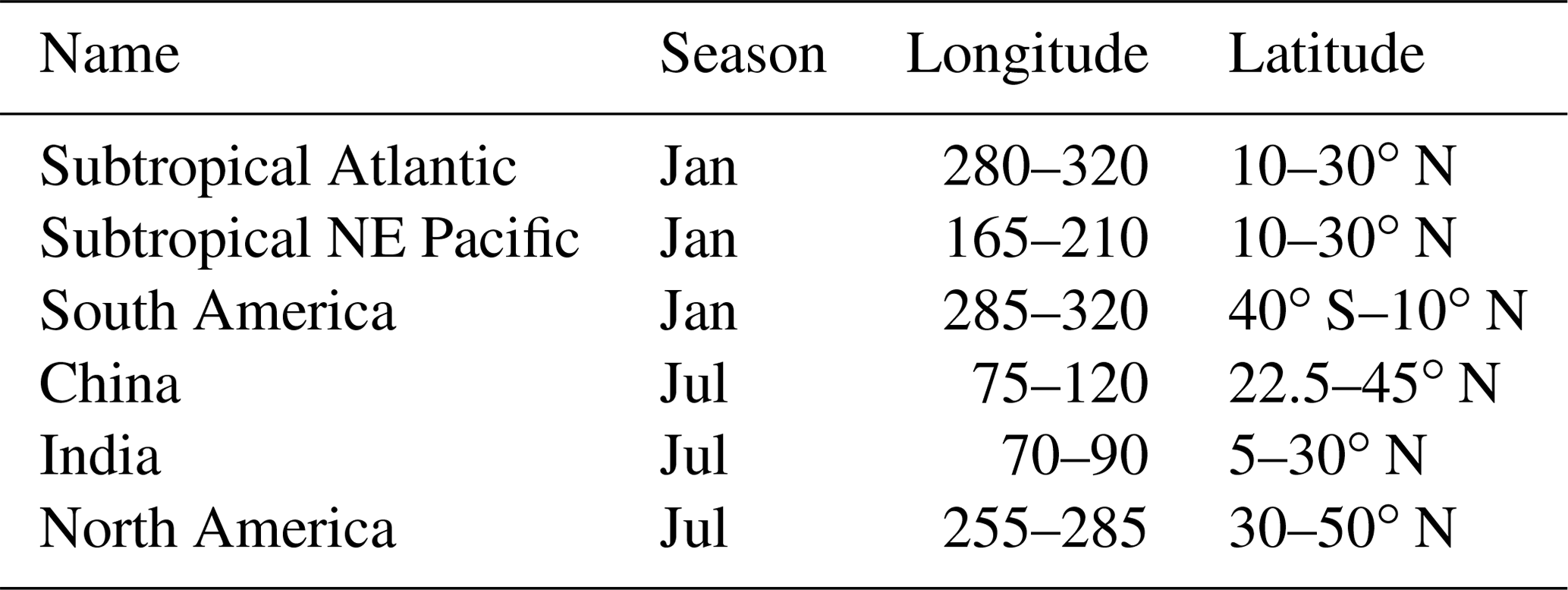
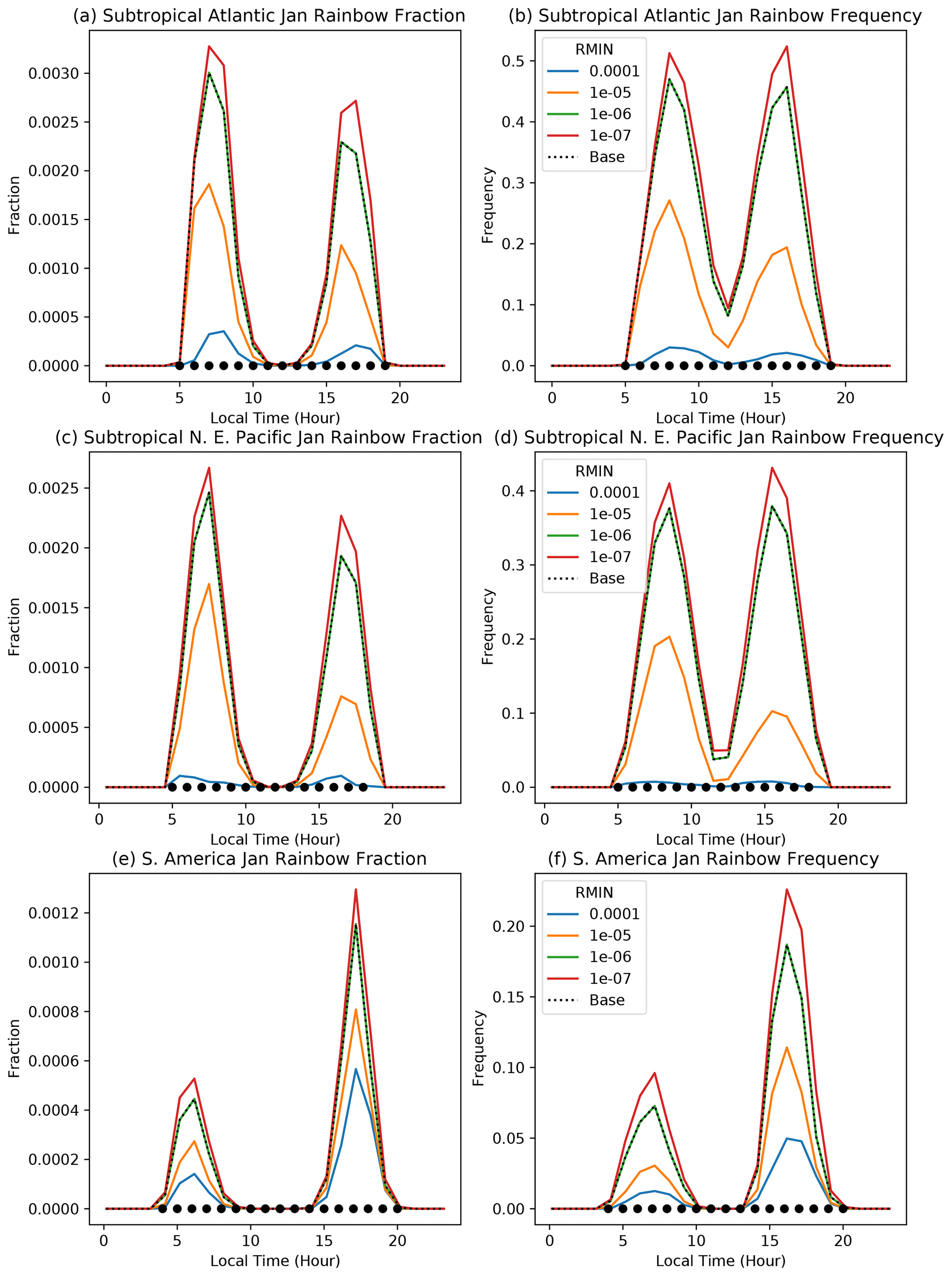
Figure 6 Diurnal cycle of rainbow fraction (a, c, e) and frequency (b, d, f) for three locations in January. Illustrated are calculations with different values of the minimum rain fraction necessary for a rainbow (RMIN). Different regions in different rows: subtropical Atlantic (a, b), NE Pacific (c, d), and South America (e, f). Regions are indicated in Table 2.

Figure 6 illustrates results for three regions in January, with sensitivity tests for the minimum rain mass for a rainbow (r_min). The base value used in Sects. 3.2 and 4.1 is shown with a dotted line in all the figures (it will overlay one of the sensitivity tests, in this case 10⁻⁶ kg kg⁻¹). The plots are in local time, with a solid circle indicating daylight hours. Due to the averaging over a month, occasionally some rainbows will be seen beyond the circles. Generally, there is a pretty consistent and strong sensitivity of the rainbow fraction and frequency to the minimum rain mass needed for a rainbow for $r_{\min }>{\mathrm{10}}^{-\mathrm{6}}$, but not for lower values. One main feature is that the diurnal cycle is unchanged, but the fraction and frequency are just scaled, though there are some differences in the relative peaks between morning and afternoon, as well as differences in sensitivity between regions, with less sensitivity over the land region of South America (Fig. 6e and f).

Expected relationships between rainbows and the diurnal cycle are seen in different regions. Over the subtropical Atlantic (Fig. 6a) and Pacific (Fig. 6c) oceans there are peaks in rainbow fraction in the morning and afternoon, with slightly more rainbows seen in the morning, consistent with the diurnal cycle in oceanic rain peaking in the morning. However, over South America (Fig. 6e and f) there is a much stronger afternoon peak in rainbow fraction and frequency, consistent with our understanding of the diurnal cycle of precipitation over land.

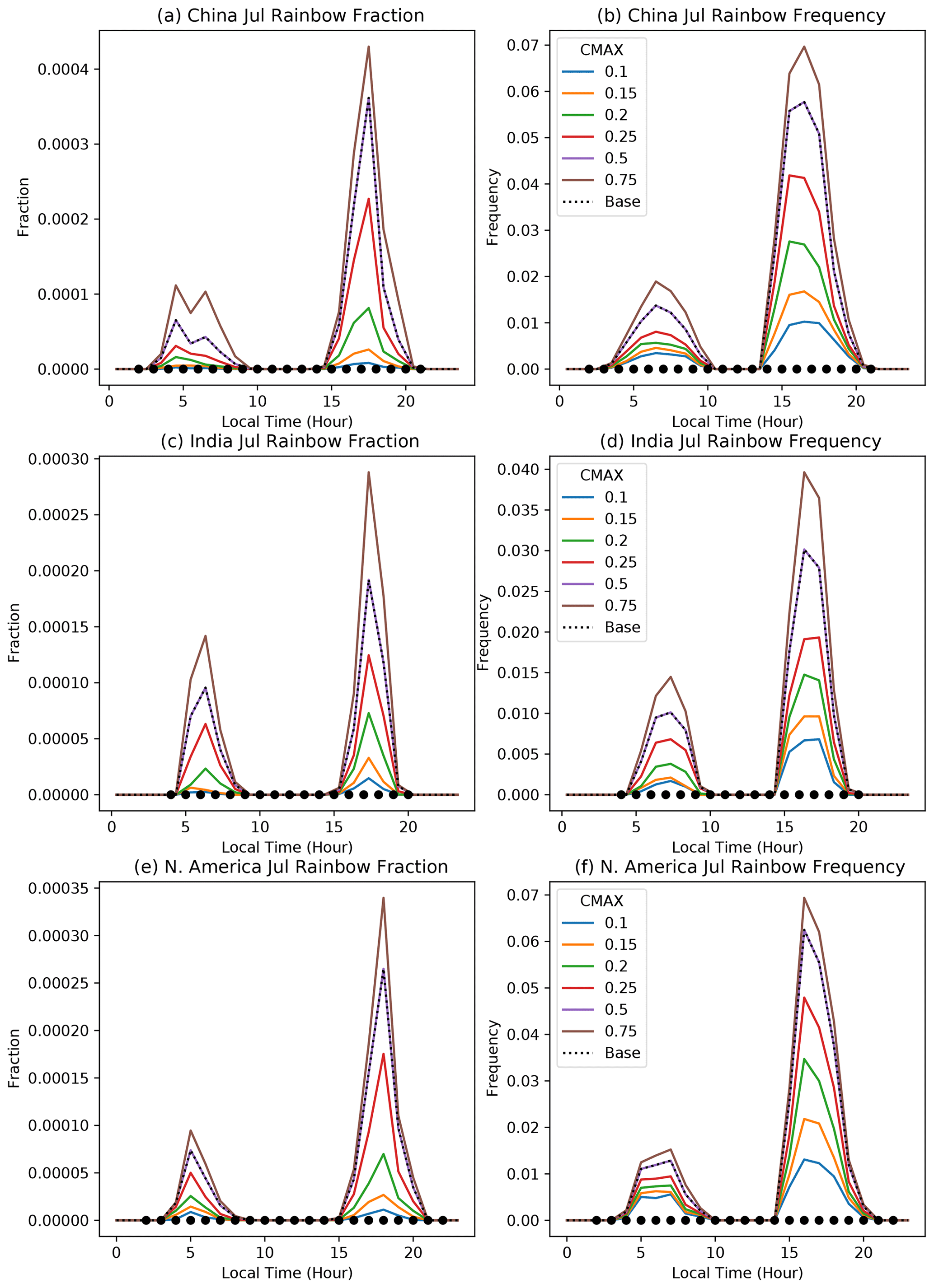
Figure 7 Diurnal cycle of rainbow fraction (a, c, e) and frequency (b, d, f) for three locations in July. Illustrated are calculations with different values of the maximum allowed cloud fraction (CMAX). Different regions in different rows: China (a, b), India (c, d), and North America (e, f). Regions are indicated in Table 2.

Results for c_max, the maximum allowed cloud fraction, in January show similar results: the same diurnal peaks by region, unchanged timing for different sensitivities, and strong sensitivity which we will analyze for July below (see Fig. 7). Sensitivities of rainbow fraction and frequency to rc_min and p_min are small (not shown). This indicates that the minimum convective precipitation is not as important as the minimum stratiform precipitation in the model for rainbow formation or that a wider range was chosen for the stratiform precipitation. It also indicates that the diagnostic is not sensitive to how deep a portion of the lower atmosphere is examined for rain and cloud. The rc_min and p_min sensitivity is also low in July, as discussed next.

Figure 7 illustrates three different regions and their sensitivities to the maximum allowed cloud area (c_max) for July. Regions chosen are over land in the Northern Hemisphere summer. Over midlatitudes of China (Fig. 7a and b) and North America (Fig. 7e and f), there is a much more significant evening peak. Rainbow fraction peaks about an hour later (18:00 vs. 17:00 local time) over North America than China. Over India (Fig. 7c and d) there is also a stronger afternoon peak but higher relative frequency in the morning. The quantitative results are sensitive to the value of c_max, with almost an order of magnitude difference between rainbow occurrence (frequency or fraction) between c_max = 0.1 and c_max = 0.75. The default value (c_max = 0.5) was chosen based on anecdotal observations over North America indicating that rainbows can be seen with fairly significant low-cloud coverage. This is a bit different than observations of rainbows by Carlson et al. (2022) correlated with cloud coverage from reanalysis (their Fig. 3a), which shows rainbows all the way up to c_max = 1 using reanalysis cloud cover data (which thus seems subject to errors).

We have also performed some experimentation looking at maps of where rainbows occur with the different parameters. Results (not shown) indicate that the sensitivity tests quantitatively change the diagnosed frequency and fraction but do not qualitatively change the location or relative magnitudes between different locations. Note that with respect to the observations from Carlson et al. (2022) examined in Fig. 4, the current parameterization produces the “high end” of rainbow frequency or fraction, and it could be adjusted by increasing the maximum allowed cloud fraction and lowering the rain threshold. This would increase the frequency of rainbows by 10 %–25 % in each case.

4.3 Climate change and rainbows

Next we assess whether anthropogenic perturbations to clouds and climate will impact simulated rainbows. We set up identical 4-year global simulations but for two different configurations. The first is identical to the control simulations, but with anthropogenic emissions of particulates (aerosol) and precursors set back to 1850 (pre-industrial or PI) conditions. This tests whether atmospheric pollution affecting clouds would have altered rainbow frequency or fraction. Second, we can simulate climate change in an uncoupled (no dynamic ocean) atmosphere–land model by doubling the CO₂ concentration and uniformly increasing the sea surface temperatures by 4 ^∘C (SST4K). The PI configuration is commonly used to examine anthropogenic aerosol effects on climate, especially through changes to cloud properties (Bellouin et al., 2020). The SST4K configuration is a common method to assess climate responses and feedbacks in the atmosphere (Cess et al., 1989).

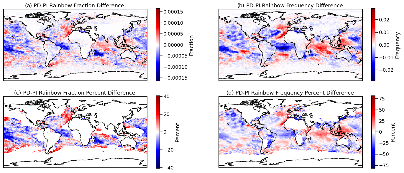
Figure 8 Annual mean absolute (a, b) and percent (c, d) difference in rainbow fraction (a, c) and frequency (b, d) between present-day (PI) and pre-industrial (PI, 1850) aerosol emissions. Percent differences are only shown when PD rainbow frequency is greater than 0.01 and rainbow fraction is greater than 0.0002.

Since aerosols are the sites on which cloud drops form, more aerosols increase cloud drop number and brighten clouds (Twomey, 1977), with subsequent adjustments to cloud fraction, lifetime, and/or water mass possible (Albrecht, 1989; Bellouin et al., 2020). Simulations with PI (1850) aerosols will have lower concentrations of cloud drops within clouds and, as a result, dimmer clouds (brighter in the present day). Figure 8 illustrates the absolute (top row) and percent (bottom row) change in rainbow fraction (left column) and frequency (right column) between the present-day (PD) control run (as in Sect. 4.1) as well as a PI aerosol emissions simulation. Most of these changes if significant would be in the Northern Hemisphere. There are slightly higher changes in the Northern Hemisphere. The lower panel shows percent differences, with a threshold for when the rainbow frequency is greater than 0.01 and rainbow fraction is greater than 0.0002. These results indicate whether historical changes in clouds due to aerosol have affected rainbows. Maximum decreases of the order of −20 % are found in regions of high rainbow frequency (compare to Fig. 3) over oceans. Changes over land are generally decreases. Note that these changes do not come from any direct scattering of sunlight due to increased particulate, which is not accounted for in the rainbow diagnostic. Also note that rainbow frequency changes are larger than differences in fraction (the scale in Fig. 8d is larger than in Fig. 8c).

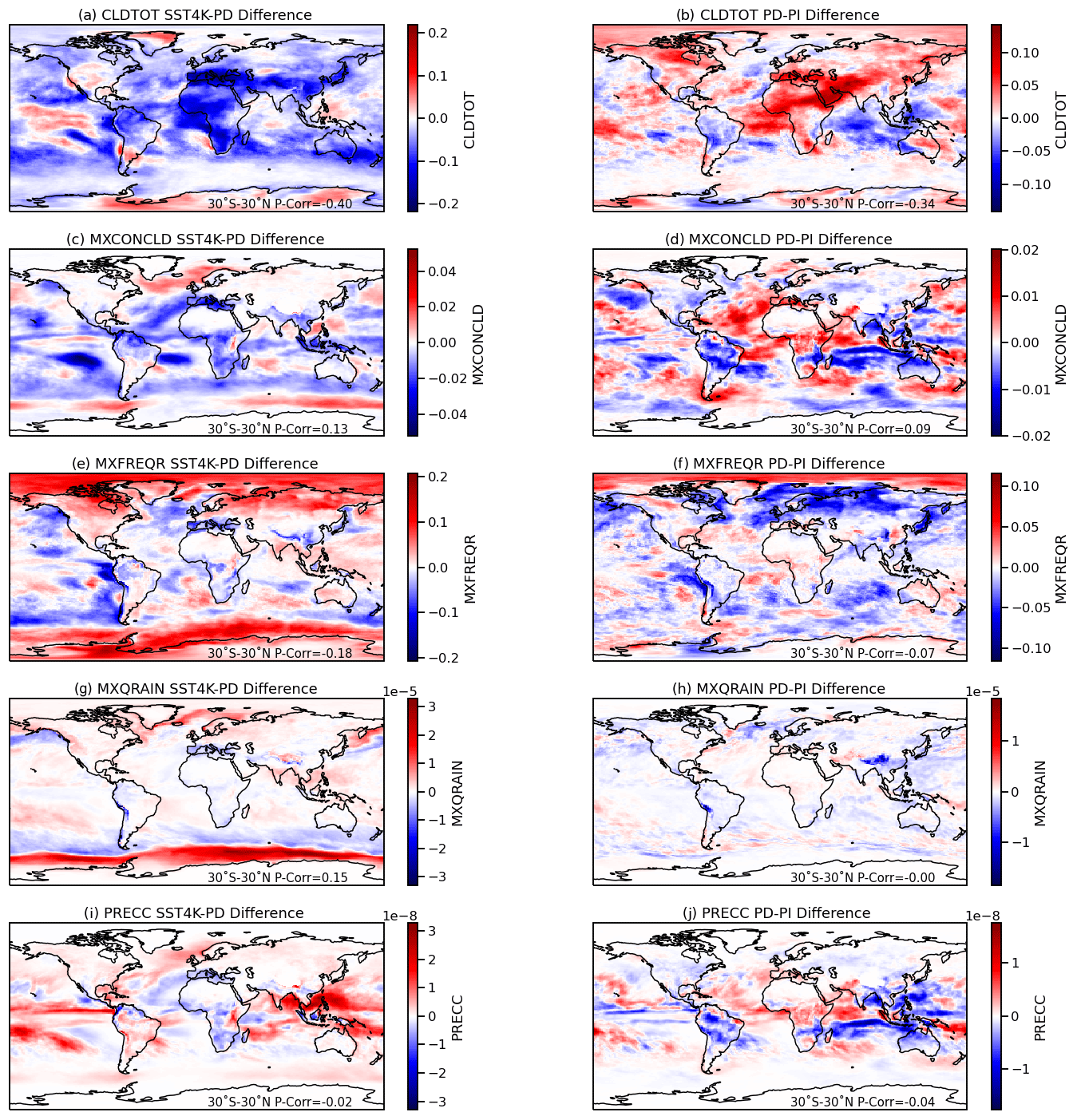
Figure 9 Annual mean absolute differences in the input fields to the rainbow parameterization for SST4K present day (PD) (a, c, e, g, i) and PI–PD (b, d, f, h, j). Shown are (a, b) total cloud cover (CLDTOT), (c, d) maximum convective cloud cover (MXCONCLD), (e, f) maximum rain fraction (MXFREQR), (g, h) maximum rain mixing ratio (MXQRAIN), and convective precipitation rate (PRECC). Numbers at the bottom indicate the Pearson pattern correlation coefficient between the differences in Figs. 8 and 10 averaged over 30^∘ S–30^∘ N.

Figure 9 provides an assessment of why the changes are occurring. The figure represents the difference in mean fields for each of the inputs into the rainbow parameterization between the two runs in Fig. 8 in the right column. We additionally take the pattern (Pearson) correlation between these differences and the rainbow fraction difference as a gauge of what changes might be affecting the rainbow diagnostics. The pattern of differences is most closely related to changes in cloud fraction, with increases in cloud fraction contributing to a reduction in rainbows. Decreases in rainbows over Northern Hemisphere land are associated with increases in cloud fraction. There is little change in the Southern Hemisphere midlatitudes as expected. It also makes sense that the frequency changes are larger: frequency is a function of cloud fraction and rain, while fraction includes rain fraction (Sect. 3.2).

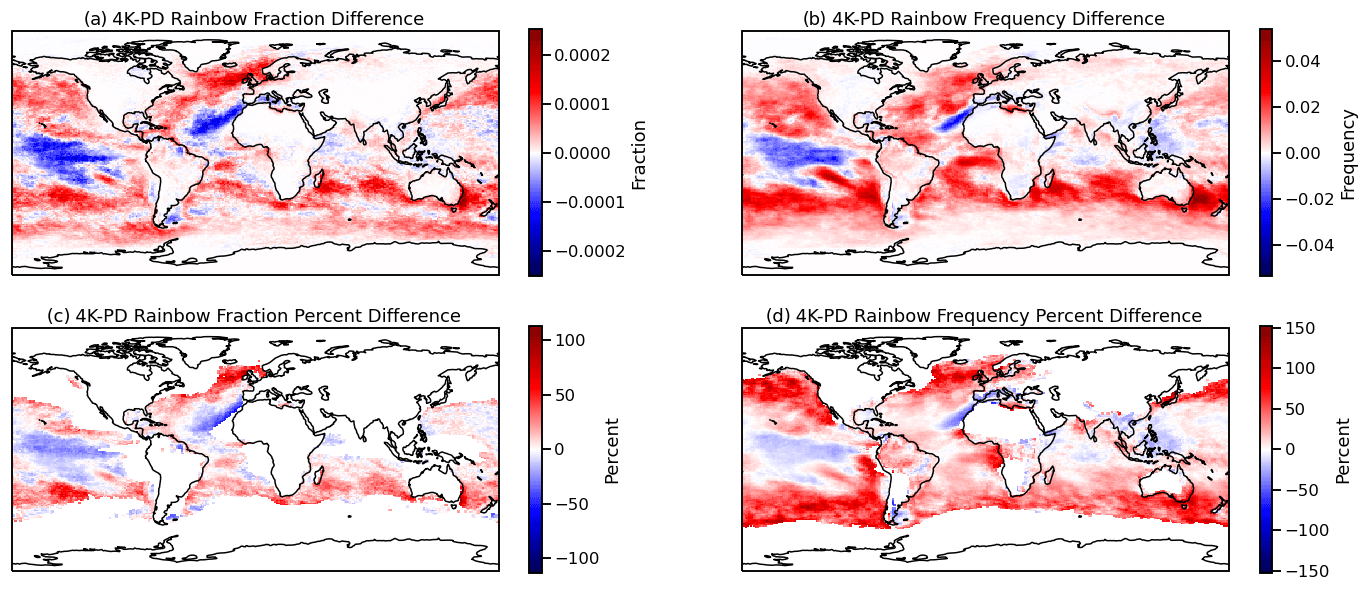
Figure 10 Annual mean absolute (a, b) and percent (c, d) difference in rainbow fraction (a, c) and frequency (b, d) between “climate change” simulations with 2×CO₂ and SST + 4 ^∘K as described in the text. Percent differences are only shown when PD rainbow frequency is greater than 0.01 and rainbow fraction is greater than 0.0002.

Finally, Fig. 10 illustrates the impact of climate change (increases in CO₂ and temperature) on the frequency of occurrence of rainbows. Rainbow fraction and frequency generally increase, with larger percent increases in rainbow frequency. Increases are small but consistent over land. Rainbow fraction increases by 30 %–50 %, with rainbow frequency in the subtropics and midlatitudes over ocean nearly doubling in some locations. As indicated in Fig. 9, this is mostly due to reductions in cloud cover as the planet warms (Fig. 9a), with a pattern correlation coefficient in the tropics of −0.4. In addition, there are some tropical oceanic regions with decreasing rainbow frequency, and these regions have increasing cloud and rain fraction. Indeed, the correlation with maximum rain and rain frequency might be a correlation with cloudiness, and the correlations with rainbows might be a bit fortuitous.

The results are broadly consistent with changes in rainbows hypothesized by Carlson et al. (2022) by applying a machine-learned rainbow model to future climate model output. Small increases in rainbow frequency were found over land and attributed to increases in rain and decreases in cloudiness. Some of the spatial patterns (increases over Indonesia, decreases over South America) are also consistent. This is not unexpected as both methods rely on the same future dataset (climate models).

5 Discussion

The rainbow diagnostic parameterization represents most of the major intuitively expected features of where and when rainbows form. There is a strong constraint on the diagnostic from the basic physics, which constrains the sun angle and requires the presence of sun (partial cloudiness) and rain. This basic physics yield many of the resulting features of the regions, seasons, and timing of the occurrence of rainbows. Simulated rainbow occurrence has broad fidelity to expected locations and diurnal cycle relationships. In regions with lots of precipitation throughout the year (like Hawaii), there are actually more rainbows with lower sun angles than higher sun angles, but in other regions the seasonal cycle of precipitation dominates. There are some complex seasonal cycles in different regions that could be explored. The diagnostic is quantitatively sensitive to the assumptions for small amounts of stratiform rain and for the maximum cloud fraction permitted for a rainbow to exist, but it is not sensitive to convective rain and the lower-layer height.

One of the most critical “needs” is a better dataset for evaluation of the rainbow diagnostic. We have made qualitative comparisons with diurnal cycles over land and ocean and attempted quantitative comparisons with a dataset developed by machine-learning the weather conditions for rainbows from limited observations. Comparisons are encouraging (particularly the pattern), with lower quantitative frequency than the observations. Adjustments could be made to better match the observations, but this would require pushing the parameterization to the edge of the sensitivity range. This is a common conundrum for developing representations of phenomena. In this case the observations are likely highly uncertain (with possible selection bias), so we refrain from excessive tuning. Datasets or archives of all-sky camera imagery from key locations could be used to find rainbows with image processing and calculate the frequency and fraction. This would have the advantage of being unbiased (continuous cameras) at a limited number of sites and used to help calibrate other methods. Such cameras would also enable detection of cloud coverage. Combined with good rain observations from co-incident gauges or ideally from rain radar to sample the field of view of the camera, this set of observations (rainbows, clouds, and rain) could constrain key parameters. This illustrates how a set of observations can be designed to test parameterizations at the right scale.

It is important to consider the scales of validity of the rainbow diagnostic. Many diagnostics or parameterizations make fundamental assumptions about the state of the atmosphere that are only valid at certain space scales and timescales. The diagnostic as developed for rainbows assumes that the rain, clouds, and the observer are all in the same grid box of the atmosphere and that no other information is needed from adjacent columns. The rainbow itself is seen by an observer but caused by rain in the same grid volume. This assumption is certainly valid for the 100 km scales of a climate model analyzed here. But, given that CESM is now being run for resolutions down to 3 km (Huang et al., 2022), it is important to consider where the parameterization is valid and whether it can be made to be scale-selective (sometimes called scale-aware). A rough estimate is that the rain and observer need to be in the same grid box as conceived here. But maybe that is not a problem as the potential rainbow would just be associated with a grid box that contains rain. The larger issue is that partial cloudiness is assumed, and for small-scale models, clouds in a volume are either on or off. At that point, the parameterization would not work, and a non-column (“3D”) treatment of rainbows would be necessary. This could be as simple as just looking for no cloud in the adjacent grid box in the direction of the sun or as complex as using 3D radiative transfer for ray tracing from the sun to rain and back to an observer. Another approach for use in high-resolution model configurations would be to simply apply the rainbow diagnostic to a coarser grid with averaged quantities and partial cloud fraction.

6 Conclusions

A combination of basic physics, geometry, and simple assumptions is effectively able to diagnose the potential for when and where rainbows would form in a GCM. The assumptions made in the development of the diagnostic parameterization and the different steps are similar to the way that other parameterizations are developed. The discussion starts with basic equations. It goes further with offline analysis with snapshots of model output, then iterating over different parameter representations. Like many other formulations in a GCM, the parameterization has limits. The results agree very well qualitatively with limited available global observations derived from machine learning and social media imagery, with less frequency than “observed”. Given selection bias in the observations, this may not be surprising. There is a need for more evaluation data, and they may need to be reformulated for models with small horizontal space scales, where the single-column assumption breaks down. The diagnostic for rainbows is a good example of how complex phenomena can be represented using the existing state of a GCM and the need for understanding the limits of those formulations.

Rainbows are not just an interesting optical phenomenon but provide important integrated metrics about key atmospheric processes. In particular, rainbows provide a simple illustration or diagnostic of the diurnal cycle of clouds and precipitation, as well as a segmentation of regimes (afternoon vs. morning rainbows, for example). The representation of rainbows is found to be quantitatively sensitive to the assumed amount of cloudiness and the amount of stratiform rain. Neither affects the location or timing of the formation of a rainbow: only the potential frequency and fraction. Rainbows are seen in expected locations in the subtropics over the ocean where broken clouds and frequent precipitation occur. The diurnal peak is in the morning over ocean and in the evening over land. Sensitivity tests show little sensitivity to the diurnal structure or pattern of rainbows, mostly just to the quantitative fraction and frequency of occurrence.

This diagnostic enables analysis of simulations for aerosol forcing and climate change. Rainbows are projected to have decreased, mostly in the Northern Hemisphere, due to aerosol pollution effects increasing cloud coverage since pre-industrial times (1850). In the future, continued climate change forcing is projected to decrease cloud cover, associated with a positive cloud feedback. The change in cloud cover is a general result for many climate models (Zelinka et al., 2020). Given that the rainbow diagnostic is sensitive to cloud cover (Fig. 7, c_max), the rainbow diagnostic projects that rainbows will increase in the future, with the largest changes at midlatitudes. These results seem consistent with sensitivity tests of the diagnostic. They are also consistent with use of the machine learning model by Carlson et al. (2022), which is not surprising since both projections are based on climate model output with similar future trends. More observations are needed to evaluate these results and refine the parameterization to be more quantitatively correct. A likely source of such data would be all-sky camera imagery with machine learning to find rainbow frequency and fraction at a series of stations. The limitation is that most of these locations would be over land, with a majority of rainbows found over the ocean. It would also be interesting to use this diagnostic in other Earth system models to assist in evaluation of cloud and rain formation.

Appendix A: Rainbow diagnostic description

Here we provide more details and some examples of how the rainbow diagnostic was developed, with a case study using instantaneous fields for 8 January at 12:00 UTC, as well as a description of the testing strategy and some supplemental plots of the seasonal cycle.

A1 Steps for parameterization

So what does it take to build a parameterization in a climate model? First is an understanding of the underlying physics. For rainbows, this is described in the text in Sect. 2. Second is the understanding of how the necessary physics are, or are NOT, described in a given model system. Then comes building a description of the physics consistent with the model system. All too often this is done implicitly, without explicit understanding of the limits of the parameterization assumptions. We will try to make this explicit.

But the theoretical concept of parameterization belies an engineering aspect to development. The parameterization must be tested for algorithmic correctness (are the equations translated corrected), numerical stability, and the wide range of physical states found in a model. This applies whether the parameterization is theoretical (based on an equation) or empirical (a fit to data). Note that empirical parameterizations can be as simple as a linear (or nonlinear) regression or as complex as a neural network, and the data can be either observations or another (often theoretical) model. See Gettelman et al. (2021) for examples of this for the warm rain formation process or Carlson et al. (2022) for how this was recently applied to rainbows.

Often this testing is done in a hierarchy of models, ranging from simple to complex (Jeevanjee et al., 2017). One often used tool for physical processes in a model is the single-column model (SCM) wherein atmospheric motions are prescribed or forced and physical parameterizations are allowed to interact. SCMs range from single-column energy balance models (Manabe and Wetherald, 1967) to complete representations of the processes in a general circulation model (e.g., Gettelman et al., 2019a). SCMs are used when interactions between processes are important. For diagnostic outputs that do not feed back on the model state (e.g., radar reflectivity or rainbows), often states of the model are used to run the parameterization offline (e.g., the Parallel Offline Radiation Tool – PORT, Conley et al., 2013). We use the offline approach here.

At these various steps, there is often evaluation against observations for various outputs, ranging from direct comparisons (e.g., against radar reflectivity form observations) to indirect comparisons of emergent states of the climate system that result from parameterized processes (e.g., top-of-the-atmosphere radiation budgets). Comparisons can use methods from simple statistical methods to complex emulation of data.

Finally, evaluations are often conducted to understand (and optimize) the sensitivity of resulting behavior from the parameterization against those observations. Sometimes this is called tuning (Hourdin et al., 2016). At the root of most parameterizations are uncertain “parameters”, whether an on/off threshold, the slope of a linear regression, or the complex weights of a neural network. Sensitivity tests and optimization can be conducted again on a single feature of the climate state or system or on a set of quantitative metrics. Section 4.2 explores the sensitivity of the scheme to the different parameters, and Sect. 4.1 illustrates a comparison against the most relevant available data, as well as qualitative evaluation based on rainbow features.

The basic physics are detailed in the main text. Here we provide more illustration of the algorithm with an example snapshot.

The diagnostic parameterization was developed by outputting individual instantaneous time slices of full 2D and 3D fields. The algorithm was first coded offline in Python to develop the logic. This took about 10 different iterations to design. Sensitivity tests of parameters were also coded offline as described in the main text. Only then was the algorithm translated into FORTRAN and implemented in the model, testing, and debugging, first in a single-column framework (Gettelman et al., 2019b) and then in full simulations.

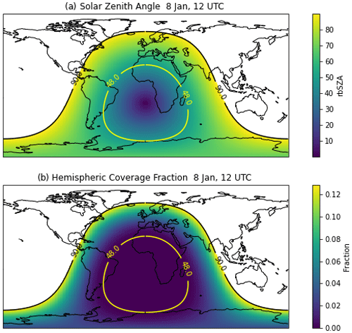
Figure A1 (a) Solar zenith angle (θ_z) on 8 January at 12:00 UTC. (b) The hemispheric fractional coverage of a rainbow seen at the same date and time. Shown are the horizon of θ_z = 90^∘ (black) and the minimum θ_z for rainbow visibility at the surface of θ_z = 48^∘ (yellow).

A2 Description

First, we need to limit the sun angle (θ_z) to within 42^∘ of the horizon. In the model, θ_z is measured from the zenith directly overhead, so at the horizon θ_z = 90^∘. Figure A1a illustrates the distribution of θ_z for 8 January at 12:00 UTC, with lines marking 90 and 48^∘. Daylight at this time is when θ_z < 90^∘. The band when rainbows are possible due to the sun angle is between these lines (48^∘ < θ_z < 90^∘). This is summer in the Southern Hemisphere, with the sun centered overhead at about 25^∘ S and 180^∘ E. Rainbows could be found at any time of the day at 75^∘ S, in morning and afternoon at 25^∘ S, and throughout all the limited daylight hours from 25–65^∘ N when the sun is never more than 42^∘ above the horizon.

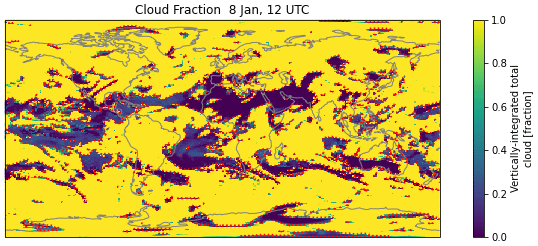
Figure A2 Total cloud fraction on 8 January at 12:00 UTC. The red dashed line is the 0.5 contour.

Note that if we want to be able to scale rainbow fractional coverage by size (see below), we need to know how much of the sky a rainbow could cover. This again comes from geometry. A maximum rainbow size will occur when the sun is on the horizon (θ_z = 90^∘), and it will occupy a hemispheric cap of the sky of 42^∘, diminishing to zero when θ_z = 48^∘ (Fig. 1b and c). Solid angle theory allows the determination of the fractional sky covered by a spherical cap for angle ϕ as $(\mathrm{1}-\text{cos}(\mathit{\varphi }\left)\right)/\mathrm{2}$, where ϕ = θ_z − 48^∘ for 48^∘ < θ_z < 90^∘. This functional form is illustrated in Fig. A1b, with a maximum fractional area of 0.13 at θ_z = 90^∘.

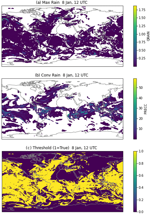
Figure A3 Instantaneous values on 8 January at 12:00 UTC. (a) Maximum stratiform rain mixing ratio (g kg⁻¹) and (b) convective precipitation rate (mm d⁻¹). Values are only shown when larger than thresholds for (a) r_min and (b) rc_min as described in the text (otherwise, they are white). (c) Map of rain passing the threshold in yellow (either a or b has values).

Second, there must be some clear sky in the grid box, so we must set a maximum on the cloud fraction. Thus the maximum total cloud fraction of either convective (A_c) or stratiform (A_s) must be less than some value c_max. CAM6 provides this total cloud cover already maximally overlapped. This total cloud fraction for the same time as Fig. A1 is illustrated in Fig. A2. We pick an initial threshold of 0.5 for c_max in Fig. A2. Essentially the cloud cover is high over most of the planet (yellow), with smaller totally and partially clear regions (green to dark blue). Only in the totally or partially clear regions is a rainbow possible with this threshold.

Third, we require a minimum amount of precipitation in the grid box. For stratiform (large-scale) precipitation (q_rs), which is prognostic and present in each layer of the atmosphere, we set a minimum stratiform mixing ratio r_min. We pick a range of pressures to sample to look for rain near the surface, selecting a minimum pressure p_min for the top of the “near-surface” layer. For convective precipitation (P_c) we only have the surface flux, so we set a minimum convective rain rate rc_min. If either of these is satisfied, then a rainbow is permitted. As an initial test we set r_min = 0.001 g kg⁻¹ and rc_min = 5 mm d⁻¹ with p_min = 850 hPa.

Figure A3 illustrates the different rain rates (Fig. A3a and b) and the threshold criteria (Fig. A3c). In Fig. A3a and b, only rain above the threshold is shown. Since this is grid-box-averaged rain, the actual mass or surface rate is higher for partial cloud cover. There is some nonzero stratiform rain over most of the oceans (Fig. A3a), in line with nearly consistent light rain in CAM6, a common bias with many models (Stephens et al., 2010). Convective rain is found more concentrated in the tropics (Fig. A3b). If either of these thresholds is met, then the rain criteria are satisfied as true (1 in Fig. A3C), which again occurs over most of the tropical oceans.

Given the four parameters c_max, p_min, r_min, and rc_min, a rainbow exists in a volume when

1. 90^∘ > θ_z > 48^∘,

2. $\text{max}(A_{\mathrm{c}},A_{\text{sr}})<c_{\max }$,

3. (P_c>rc_min) or (q_rs>r_min),

where A_c, A_sr, and q_rs are the maximum over model levels from the surface to p_min.

This defines the rainbow frequency of occurrence. As noted in the text, we also want to determine how much of the sky a rainbow may occupy. To determine the fraction of sky coverage of a rainbow we use the spherical geometry of how much of a hemisphere the rainbow could occupy and a fractional occurrence of rain (A_r). A_r is given by the maximum of the stratiform rain fraction (A_sr) and the convective cloud fraction (A_c) in the lower atmospheric layer defined by p_min:

$$A_{\mathrm{r}}=\text{max}(A_{\text{sr}},A_{\mathrm{c}}).$$

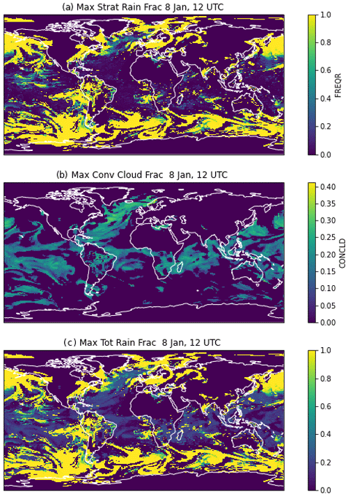
Figure A4 Instantaneous values on 8 January at 12:00 UTC. (a) Stratiform rain fraction, (b) maximum convective cloud fraction, and (c) total rain fraction as the maximally overlapped combination of (a) and (b).

Figure A4 illustrates the maximum near-surface stratiform rain area max(A_sr) (Fig. A4a), the maximum near-surface convective cloud area, max(A_c) (Fig. A4b), and the maximum total rain fraction A_r (Fig. A4c). Note that the stratiform fraction is much higher, and the scales in Fig. A4a and A4b are different.

The fractional area of a rainbow Frac_RB is the fraction of the hemisphere for a spherical cap of angle θ_z − 48^∘ multiplied by the rain fraction (A_r) derived above.

$$\begin{array}{ll}{\displaystyle }& {\displaystyle }{\mathrm{Frac}}_{\mathrm{RB}}=\mathrm{0}\text{ for }{\mathit{\theta }}_z>\mathrm{48}{}^{\circ }\\ {\displaystyle }& {\displaystyle }{\mathrm{Frac}}_{\mathrm{RB}}=\left(\left(\mathrm{1}-\text{cos}\left({\mathit{\theta }}_z-\mathrm{48}{}^{\circ }\right)\right)/\mathrm{2}\right)\times A_{\mathrm{r}}\text{ for }\mathrm{48}{}^{\circ }>{\mathit{\theta }}_z>\mathrm{90}{}^{\circ }\\ {\displaystyle }& {\displaystyle }{\mathrm{Frac}}_{\mathrm{RB}}=\mathrm{0}\text{ for }{\mathit{\theta }}_z>\mathrm{90}{}^{\circ }\end{array}$$

A3 Development and testing strategy

The representation of rainbow frequency of occurrence (Freq_RB) and fractional coverage (Frac_RB) is purely diagnostic (it does not feed back on the model state). Thus the parameterization can be easily developed “offline”. CAM6 is run in a standard configuration (100 km, 32 levels) for 1 month, with instantaneous output every time step (30 min) for the required cloud, rain, and solar angle fields. The output is then used to analyze and test the parameterization offline. The algorithm described above is not the only possible description of a rainbow, and other forms of the parameterization with more or fewer steps were tried. For example: the fraction of rain in a grid box could also be considered a threshold value, but this involved assumptions about the convective rain area in the model. For this case, an “Occam's razor” approach is used to simplify the representation as much as possible and minimize the number of parameters.

Testing was conducted offline, and then the resulting parameterization coded back into the model, in the interface to the cloud microphysics routine, where it will eventually become a small stand-alone diagnostic code. The product is numbers: a fractional area coverage of a rainbow in each grid volume at each time (Frac_RB), and a frequency flag set to 1 if there is a rainbow and zero if not (Freq_RB). The average of that flag over a time period yields the frequency of occurrence. The advantage of this approach is that the model test run can be conducted again with the in-line calculations for Frac_RB and Freq_RB and validated against the offline estimate for debugging purposes. It also enables rapid offline sensitivity tests to be developed. Table 1 lists the default parameter values and ranges selected for the sensitivity tests in the text.

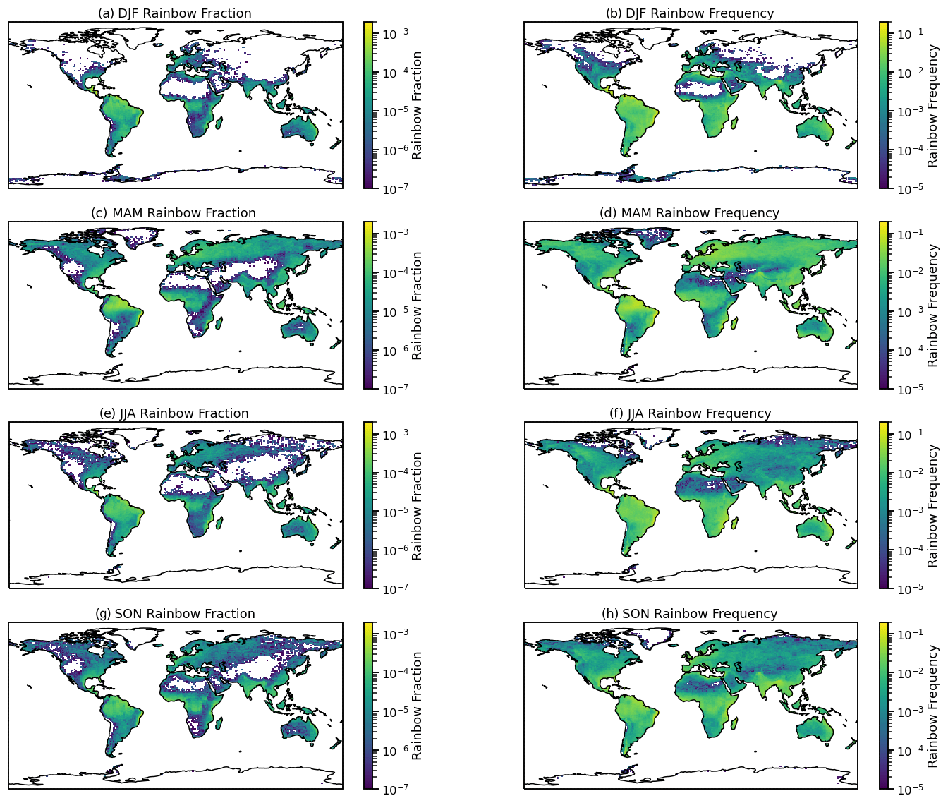
Figure A5 Seasonal average diagnosed land-only rainbow fraction (a, c, e, g) and frequency (b, d, f, h) for different seasons. (a, b) December–February (DJF), (c, d) March–May (MAM), (e, f) June–August (JJA), and (g, h) September–November (SON).

A4 Seasonal cycle over land

The seasonal cycle over land is illustrated in Fig. A5 from 4-year climatological simulations. There is little rainbow frequency over Northern Hemisphere land in winter (DJF, Fig. A5b) and a peak frequency in spring (MAM, Fig. A5d), particularly over Europe and Asia. The tropics have relatively high frequency all year. Fraction adds the sky coverage and is higher for low sun angles (e.g., the discussion of a winter peak in Hawaii above). So the combination means rainbow potential fraction peaks in Northern Hemisphere spring, including over Europe. The southeastern US has moderately high frequency in all seasons but winter. Southern Hemisphere land is generally more subtropically situated and thus has higher frequency in midlatitudes, as well as high frequency in the tropics. Southern Hemisphere arid regions seem to have a higher rainbow frequency and fraction than the Northern Hemisphere. This might be due to dry land masses over the larger continents. More evaluation based on local conditions is warranted. See the discussion of observations in the main text. In addition, we can analyze the diurnal cycle of rainbow diagnostics in key regions.