Modelling the terrestrial nitrogen and phosphorus cycle in the UVic ESCM

Nitrogen (N) and phosphorus (P) biogeochemical dynamics are crucial for the regulation of the terrestrial carbon cycle. In Earth system models (ESMs) the implementation of nutrient limitations has been shown to improve the carbon cycle feedback representation and, hence, the fidelity of the response of land to simulated atmospheric CO₂ rise. Here we aimed to implement a terrestrial N and P cycle in an Earth system model of intermediate complexity to improve projections of future CO₂ fertilization feedbacks. The N cycle is an improved version of the Wania et al. (2012) N module, with enforcement of N mass conservation and the merger with a deep land-surface and wetland module that allows for the estimation of N₂O and NO fluxes. The N cycle module estimates fluxes from three organic (litter, soil organic matter and vegetation) and two inorganic (${\mathrm{NH}}_{\mathrm{4}}^{+}$ and ${\mathrm{NO}}_{\mathrm{3}}^{-}$) pools and accounts for inputs from biological N fixation and N deposition. The P cycle module contains the same organic pools with one inorganic P pool; it estimates influx of P from rock weathering and losses from leaching and occlusion. Two historical simulations are carried out for the different nutrient limitation setups of the model: carbon and nitrogen (CN), as well as carbon, nitrogen and phosphorus (CNP), with a baseline carbon-only simulation. The improved N cycle module now conserves mass, and the added fluxes (NO and N₂O), along with the N and P pools, are within the range of other studies and literature. For the years 2001–2015 the nutrient limitation resulted in a reduction of gross primary productivity (GPP) from the carbon-only value of 143 to 130 Pg C yr⁻¹ in the CN version and 127 Pg C yr⁻¹ in the CNP version. This implies that the model efficiently represents a nutrient limitation over the CO₂ fertilization effect. CNP simulation resulted in a reduction of 11 % of the mean GPP and a reduction of 23 % of the vegetation biomass compared to the baseline C simulation. These results are in better agreement with observations, particularly in tropical regions where P limitation is known to be important. In summary, the implementation of the N and P cycle has successfully enforced a nutrient limitation in the terrestrial system, which has now reduced the primary productivity and the capacity of land to take up atmospheric carbon, better matching observations.

1 Introduction

Terrestrial biogeochemical cycles are sensitive to changes in atmospheric CO₂ concentrations and climate. Their global evolution will determine the capacity of vegetation and soils to store anthropogenic carbon (Goll et al., 2012). In terrestrial ecosystems carbon cycle feedbacks are constrained in part by the availability of nutrients (Fisher et al., 2012; Zaehle et al., 2014; Wieder et al., 2015; Du et al., 2020). Among nutrients, nitrogen (N) and phosphorus (P) are considered to be the most critical for limiting the primary productivity (Filipelli, 2002; Fowler et al., 2013). Both are fundamental functional needs for plant biochemistry, and their requirement is common in all vegetation taxa (Filipelli, 2002; Vitousek et al., 2010; Du et al., 2020). Regionally, the availability of nutrients can impair the photosynthetic efficiency of terrestrial vegetation and consequently their response to increasing atmospheric CO₂. Hence, in Earth system models (ESMs) the representation of nutrient limitations is imperative to improve the accuracy of carbon feedback projections and estimation of carbon budgets.

The simulations from first-generation ESMs with carbon-only schemes have very likely overestimated the response of the terrestrial ecosystem to the increase in atmospheric CO₂ concentrations (Hungate et al., 2003; Thorton et al., 2007), showing a high terrestrial carbon uptake response, which would require an unrealistically large nutrient supply. The addition of an N cycle to the land system in ESMs has shown an overall reduction in the effect of CO₂ fertilization, especially in high latitudes, with a weaker response in low latitudes which are typically P limited in natural systems (Wang et al., 2007, 2010; Goll et al., 2017; Du et al., 2020; Wang et al., 2020).

The global distribution of N and P is dependent on the biogeochemical characteristics of each nutrient. N inputs are mainly from biological nitrogen fixation (BNF) and atmospheric deposition with little addition from rock weathering (Du et al., 2020). There are two types of N deposition from the atmosphere: wet (precipitation) and dry (particles). Among the two, wet deposition represents most of the atmospheric N input (Fowler et al., 2013; Dynarski et al., 2019). In contrast, the main input of P comes from rock weathering (mainly apatite) with less inputs from atmospheric deposition as dust particles. These characteristics are among the reasons for a global spatial pattern where young soils are usually N limited and old soils P limited (Filipelli, 2002; Fowler et al., 2013; Du et al., 2020). N accumulates rapidly from BNF where N fixers are abundant and slowly where atmospheric deposition is dominant. Thereby, old soils have a larger accumulation of N, especially in regions where N fixers are abundant. On the other hand, P input is limited by the parent material, and the bioavailability is further constrained by the retention of recalcitrant P in soils. Walker and Syers (1976) even suggested that P storage has a fixed total that cannot rapidly be replenished, as parent material is limited.

These notions led to the common conceptualization that high latitudes are N limited, while tropical regions are P limited. While this generalization is correct in most observational studies, the complex pattern of limitation is more intricate, and P limitation could be more common than is commonly inferred. Du et al. (2020) found that globally 43 % of the terrestrial system is relatively limited by P, while only 18 % is limited by N, with the rest being co-limited by both. Biochemically, the availability of N and P can directly limit one another. The addition of P has been shown to be positive for the N fixation, leading to the replenishment of N in ecosystems (Eisele et al., 1989). N supply on the other hand regulates the production of the enzyme phosphatase that cleaves ester P bonds in soil organic matter (McGill and Cole, 1981; Olander and Vitousek, 2000; Wang et al., 2007).

Biodiversity plays a crucial role in biogeochemical cycles. The fluxes and availability of N and P in soils depend on the interactions between the soil mineral matrix, plants and microbes (Cotrufo et al., 2013). For example, N input from atmospheric N₂ fixation is mediated by a specialized group of microorganisms. Furthermore, the recycling of N from plants–soils–microbes determines the availability of N for plant uptake. Overall, the land biota dynamics impact the productivity, ecosystem resilience and stability (Yang et al., 2018). High diversity has been linked to enhanced vegetation productivity (Wagg et al., 2014). The diversity in terrestrial ecosystems is determined by biological, environmental and physicochemical processes. Anthropogenic activities can influence soil diversity, impacting the availability and cycling of N and P (Chen et al., 2019). For example, N and P fertilization has been shown to affect soil microbial biomass and composition (Ryan et al., 2009). Plant diversity is linked to soil health and functioning and is the core of the N and P cycles. Vegetation species' variable adaption to nutrient concentrations also plays a role in the availability of nutrients in soils and the biogeography of terrestrial vegetation. Overall, biodiversity constitutes an environmental resilience factor to abrupt changes (Van Oijen et al., 2020). However, implementing such dynamics remains far beyond the capabilities of the present-generation Earth system models. Several studies have found that in some ecosystems lack of N in soil usually leads to dominance of woody symbiotic N fixers (e.g. Menge et al., 2012). The availability of P is also impacted by the geochemical interactions in terrestrial soils, Vitousek et al. (2010) defined six mechanisms by which P is driven to limitation: loss by leaching; soil barriers that physically prevent access to roots; slow release of mineral P forms; P parent material; sequestration of P in soils and pools in the ecosystem; and, finally, anthropogenic input of nutrients.

Despite its importance P terrestrial limitation has been rare in Earth system modelling. The effect of P in tropical forests may be the key to better represent the vegetation biomass and the response to CO₂ fertilization. The lack of P observational data is partly responsible for the difficulty of simulating P limitation in Earth system models (Spafford and MacDougall, 2021). However, several studies have attempted to provide reliable global P datasets (Yang et al., 2013; Hartmann et al., 2014; He et al., 2021) that could be used to develop more accurate models. Furthermore, many studies have shown that the inclusion of P into ESM structures is possible and that it improves the representation of vegetation biomass in tropical regions (Wang et al., 2007, 2010; Goll et al., 2012, 2017; Fleischer et al., 2019; Thum et al., 2019; Yang et al., 2019; Wang et al., 2020; Nakhavali et al., 2022). The addition of nutrient limitation has been observed to mainly affect the capacity of vegetation to absorb carbon (Wang et al., 2010; Goll et al., 2017; Wang et al., 2020). Therefore, the accumulation of carbon in the atmosphere is enhanced, leading to increases in temperature in simulations. These temperature changes are likely to have some impact on variables' sensitivity to atmospheric temperature changes. Furthermore, the decrease in vegetation biomass impacts variables sensible to the distribution and composition of plant functional types.

Intermediate-complexity Earth system models have a lower spatial representation and model structures that have been intentionally simplified in one or more ways. This simplification allows for long-term simulations that are typically not feasible in higher-complexity models. This class of model is not suitable for studying processes at small spatial scales. Hence, they are used in research questions that require large spatial and temporal scales (Weber, 2010). Current-generation Earth system models have already developed nutrient limitation to their model structure (e.g. Community Land Model, Lawrence et al., 2019; Joint UK Land Environment Simulator, Clark et al., 2011; Community Atmosphere–Biosphere Land Exchange model, Haverd et al., 2018; Australian Community Climate and Earth System Simulator, Ziehn et al., 2020). While CN models are more common, CNP models remain rarer. However, P cycles have been suggested to be included into Earth system models for its importance in tropical regions (Wang et al., 2010; Goll et al., 2012). The first attempt to include nutrient limitation in the University of Victoria Earth System Climate Model (UVic ESCM) was done by Wania et al. (2012) but was not included in the current publicly available version of the model due to the need for further improvement. We aim to describe a terrestrial N and P cycle adapted, developed and implemented for the UVic ESCM version 2.10. The main dynamics captured in this study are in the terrestrial system, especially vegetation. Furthermore, we intend to improve the current state of the previous N cycle implemented in the UVic ESCM, develop a new P cycle, and couple carbon N and P in order to improve the carbon cycle feedback projections.

2 Methodology

2.1 Model description

The UVic ESCM is a climate model of intermediate complexity (ver. 2.10; Weaver et al., 2001; Mengis et al., 2020), and it contains a simplified moisture-energy balance atmosphere coupled with a three-dimensional ocean general circulation (Pacanowski, 1995) and a thermodynamic sea-ice model (Bitz et al., 2001). The model has a common horizontal resolution of 1.8^∘ latitude and 3.6^∘ longitude, and the oceanic module has a vertical resolution of 19 levels with a varying vertical thickness (50 m near the surface to 500 m in the deep ocean).

In version 2.10, the soil is represented by 14 subsurface layers with thickness exponentially increasing with depth with a surface layer of 0.1 m, a bottom layer of 104.4 m and a total layer of 250 m. Only the first eight layers have active hydrological processes (top 10 m); below that lies bedrock with thermal characteristics of granitic rocks. The soil carbon cycle is active in the top six layers up to a depth of 3.35 m (Avis, 2012; MacDougall et al., 2012). The soil respiration is a function of temperature and moisture (Meissner et al., 2003). The terrestrial vegetation is simulated by a top-down representation of interactive foliage and flora including dynamics (TRIFFID), representing vegetation interaction between five functional plant types: broadleaf trees, needleleaf trees, shrubs, C3 grasses and C4 grasses that compete for space in the grid following the Lotka–Volterra equations (Cox, 2001). Net carbon fluxes estimated in the model update the total areal coverage, leaf area index and canopy height for each plant functional type (PFT). For each PFT the carbon fluxes are derived from a photosynthesis–stomatal conductance model (Cox et al., 1998). The carbon uptake through photosynthesis is allocated to growth and respiration, and the vegetation carbon is transferred to the soil via litterfall and allocated to the soil as a decreasing function of depth (proportional to root distribution) and except for the top layer is only added to soil layers with temperatures above 1 ^∘C.

Furthermore, permafrost carbon is prognostically generated within the model using a diffusion-based scheme meant to approximate the process of cryoturbation (MacDougall and Knutti, 2016). The sediment processes are modelled using an oxic-only calcium carbonate scheme (Archer, 1996). Terrestrial weathering is diagnosed from the spin-up net sediment flux and stays fixed at the preindustrial equilibrium value (Meissner et al., 2012). Mengis et al. (2020) merged the previous version of the UVic ESCM and evaluated its performance representing carbon and heat fluxes, as well as water cycles and ocean tracers. A full description of the model can be found in Mengis et al. (2020).

Figure 1 Diagram representing the UVic ESCM nitrogen cycle.

2.2 Nitrogen cycle

2.2.1 Nitrogen uptake

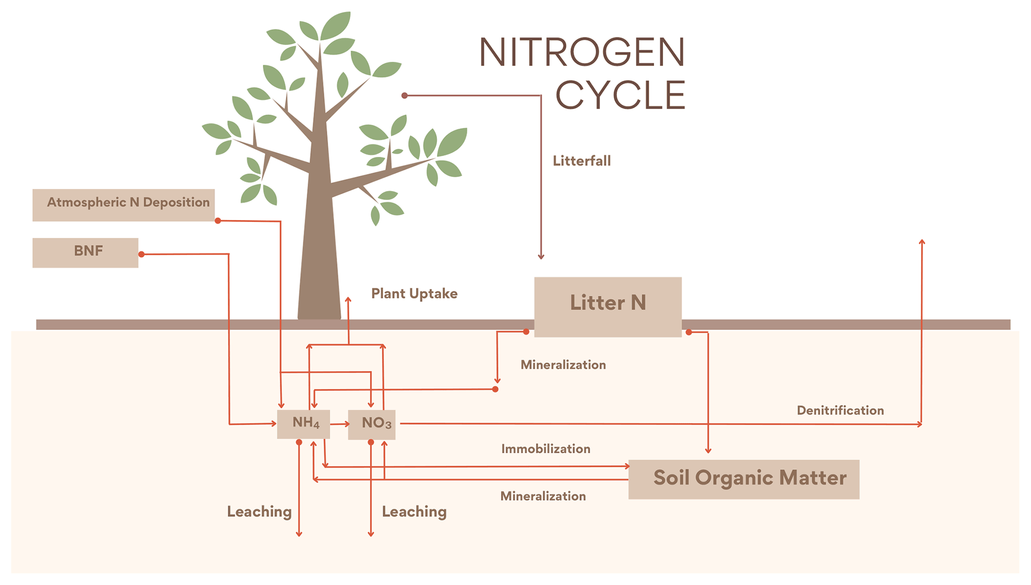
The new N cycle module was adapted from Wania et al. (2012). The module contains three organic (litter, soil organic matter and vegetation) and two inorganic (${\mathrm{NH}}_{\mathrm{4}}^{+}$, ${\mathrm{NO}}_{\mathrm{3}}^{-}$) N pools. The base structure is based on Gerber et al. (2010) with further modifications to fit the UVic ESCM scheme. ${\mathrm{NH}}_{\mathrm{4}}^{+}$ is produced both from BNF and from the mineralization of organic N and can be taken up by plants (vegetation), leached or transformed into ${\mathrm{NO}}_{\mathrm{3}}^{-}$ via nitrification. ${\mathrm{NO}}_{\mathrm{3}}^{-}$ is produced through nitrification and can be taken up by plants, leached or denitrified into NO, N₂O or N₂. The inorganic N is distributed between leaf, root and wood, with wood having a fixed stoichiometry ratio and variable ratios for the leaf and root pools. Organic N leaves the living pools via litterfall into the litter pool which is either mineralized or transferred to the organic soil pool; a part of this N can be mineralized into the inorganic N pools. At the same time N can flow from the inorganic to the soil organic pool via immobilization. The CN ratios in leaves are determined by Eq. (1):

$$\begin{array}{}\text{(1)}& {\mathrm{CN}}_{\text{leaf}}={\displaystyle \frac{{\mathrm{C}}_{\text{leaf}}}{{\mathrm{N}}_{\text{leaf}}}},\end{array}$$

where C_leaf is the carbon content in leaves, and N_leaf is the N content in leaves. CN_leaf is one of the most important nutrient limiters in the model. It controls the maximum carboxylation rate of RubisCO. Furthermore, it controls vegetation biomass. If the leaf C:N ratio is higher than CN_leafmax (the maximum CN ratio parameter), terrestrial vegetation biomass is reduced.

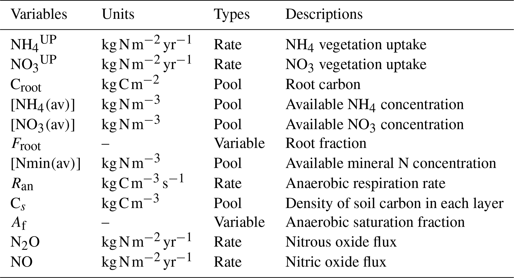
Table 1 Updated nitrogen cycle module pools, rates and variables.

The new version of the N cycle has been merged with a deep land-surface (MacDougall and Knutti, 2016) and a new wetland module (Nzotungicimpaye et al., 2021). Both inorganic N pools are transferred between soil layers following ground-water flow. Given this flow the distribution of N in layers was taken into account in the uptake calculations in Eqs. (2) and (3), and a root fraction was added (4), fixing the amount of root biomass per PFT per layer depth. The equations governing N uptake are

$$\begin{array}{}\text{(2)}& {\displaystyle }\begin{array}{rl}& {{\mathrm{NH}}_{\mathrm{4}}}^{\text{UP}}=\\ & \sum _{\text{PFT}}\left({\displaystyle \frac{V_{\text{maxn}}{\mathrm{C}}_{\text{root}}\left[{\mathrm{NH}}_{\mathrm{4}}\right(\mathrm{av}\left)\right]F_{\text{root}}}{K_{n,\mathrm{1}/\mathrm{2}}+\left[\mathrm{Nmin}\right(\mathrm{av}\left)\right]}}+\left[{\mathrm{NH}}_{\mathrm{4}}\right(\mathrm{av}\left)\right]\cdot \mathrm{Qt}\right),\end{array}\text{(3)}& {\displaystyle }\begin{array}{rl}& {{\mathrm{NO}}_{\mathrm{3}}}^{\text{UP}}=\\ & \sum _{\text{PFT}}\left({\displaystyle \frac{V_{\text{maxn}}{\mathrm{C}}_{\text{root}}\left[{\mathrm{NO}}_{\mathrm{3}}\right(\mathrm{av}\left)\right]F_{\text{root}}}{K_{n,\mathrm{1}/\mathrm{2}}+\left[\mathrm{Nmin}\right(\mathrm{av}\left)\right]}}+\left[{\mathrm{NO}}_{\mathrm{3}}\right(\mathrm{av}\left)\right]\cdot \mathrm{Qt}\right),\end{array}\end{array}$$

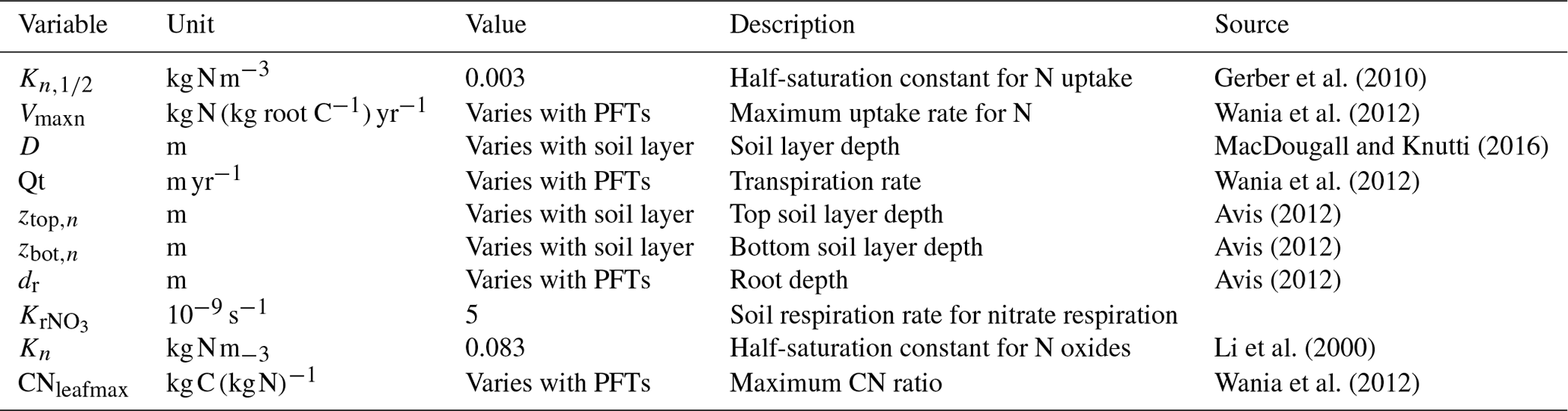
where ${{\mathrm{NH}}_{\mathrm{4}}}^{\text{UP}}$ and ${{\mathrm{NO}}_{\mathrm{3}}}^{\text{UP}}$ represent the N uptake. The left term is the active uptake, while the right term is the passive uptake (see Table 1); the latter is the transport of N via the transpiration water stream. V_maxn is the maximum uptake rate for N; C_root is the root carbon biomass; [NH₄(av)], [NO₃(av)], and [Nmin(av)] are the NH₄, NO₃, and mineral N concentrations; $K_{n,\mathrm{1}/\mathrm{2}}$ is the half-saturation constant for N; and Qt is the transpiration rate. av represents the available portion of NH₄ and NO₃ in soil. This fraction is calculated as the total concentration of NH₄ and NO₃ divided by sorption factors (10 and 1, respectively) following Wania et al. (2012). The equation for root fraction is

$$\begin{array}{}\text{(4)}& F_{\text{root},\text{PFT}}={\displaystyle \frac{e^{z_{\text{top},n}/d_{\mathrm{r},\text{PFT}}}-e^{z_{\text{bot},n}/d_{\mathrm{r},\text{PFT}}}}{\mathrm{1}-e^{D/d_{\mathrm{r},\text{PFT}}}}},\end{array}$$

where Z_top and Z_bot represent the top layer and bottom layer depth, respectively, while D and d_r are the depth of the soil layer and the root depth. The depth of the soil layer represents the depth of each specific soil layer. Root depth is a PFT-based parameter that represents the depth of the roots. Given the multiple-soil-layer setup, the root fraction modifies the value of root carbon, creating a more realistic representation of the uptake root depth reach for each PFT given the multiple-soil-layer setup.

2.2.2 Denitrification

The N cycle was merged with a wetland module that allowed for the estimation of anoxic fractions for each soil layer, based on Gedney and Cox (2003). The anoxic fraction is taken to be the saturated fraction of the soil layer that is shielded from O₂ by the saturated soil layer above. The anoxia representation led to denitrification to be added to the N model, accounting for the largest exit pathway for N in the terrestrial biosphere. The anaerobic respiration is estimated from Eq. (5):

$$\begin{array}{}\text{(5)}& R_{\text{an}}=K_{\mathrm{r}{\mathrm{NO}}_{\mathrm{3}}}{f}_{\mathrm{t}}{f}_{\mathrm{m}}{\mathrm{C}}_{\mathrm{s}}{A}_{\mathrm{f}}{\displaystyle \frac{\left[{\mathrm{NO}}_{\mathrm{3}}\right(\mathrm{av}\left)\right]}{\left[{\mathrm{NO}}_{\mathrm{3}}\right(\mathrm{av}\left)\right]+K_n}},\end{array}$$

where R_an is the anaerobic respiration, $K_{\mathrm{r}{\mathrm{NO}}_{\mathrm{3}}}$ is the ideal respiration rate via NO₃ reduction, f_t and f_m are temperature and moisture functions, C_s is the concentration of organic carbon, A_f is the anaerobic fraction, and K_n is the half-saturation of N oxides (Li et al., 2000). The temperature and moisture soil functions are taken directly from Cox (2001) and are represented by the following equations:

$$\begin{array}{}\text{(6)}& {\displaystyle }{f}_{\mathrm{t}}=q_{\mathrm{10}}^{\mathrm{0.1}(t_{\mathrm{s}}-\mathrm{25})},\text{(7)}& {\displaystyle }{f}_{\mathrm{m}}=\left\{\begin{array}{ll}\mathrm{1}-\mathrm{0.8}(S-S_{\mathrm{0}})& \text{for }S>S_{\mathrm{0}},\\ \mathrm{0.2}+\mathrm{0.5}\left(\frac{S-S_{\mathrm{W}}}{S_{\mathrm{0}}-S_{\mathrm{W}}}\right)& \text{for }{S}_{\mathrm{W}}<S\le S_{\mathrm{0}},\\ \mathrm{0.2}& \text{for }S\le S_{\mathrm{W}},\end{array}\right.\end{array}$$

where in f_t, q₁₀=2, and t_s is the soil temperature in ^∘C. In f_m, S is the soil moisture, S_W is the wilting point of soil moisture, and S₀ is the optimum soil moisture. Fluxes of N₂O and NO to the atmosphere are computed based on the “leaky pipe” conceptualization of soil–nitrogen processes (Firestone and Davidson, 1989). In the leaky pipe conceptual model N₂O and NO leak out of reactions of one species of nitrogen into another, namely nitrification (NH₄ to NO₃) and denitrification (NO₃ to N₂). The size of the holes is determined by the soil processes. For implementation in the UVic ESCM the size of the holes is fixed, but the partitioning ratio between NO and N₂O changes based on the water-filled pore space of the soil layer. The ratio is parameterized based on an empirical relationship derived by Davidson et al. (2000):

$$\begin{array}{}\text{(8)}& {\displaystyle \frac{{\mathrm{N}}_{\mathrm{2}}\mathrm{O}}{\mathrm{NO}}}={\mathrm{10}}^{\mathrm{2.6}{S}_{\mathrm{U}}-\mathrm{1.66}},\end{array}$$

where S_U is the water-filled pore space. Thus, the model produces a total flux of both NO and N₂O for nitrification and denitrification, which is partitioned between the two species based on the above relationship. The NO flux is added to the atmosphere and redeposited as part of the N deposition flux. The N₂O flux is added to the N₂O pool in the atmosphere, which has a characteristic half-life of 90.78 years (Myhre et al., 2013). Decayed N₂O is assumed to become part of the atmospheric N₂ pool.

2.2.3 Mass balance N cycle

In the Wania et al. (2012) N cycle module, under N limitation (CN_leaf>CN_leafmax), the N available was increased artificially by reducing the leaching by up to 100 % and if necessary the immobilization by 50 %. These mechanics created an unrealistic increase in N in soils and thereby defied the mass balance conservation of the module.

Here, the vegetation can no longer take up extra N from leaching or immobilization under nutrient limitation. Instead, under nutrient limitation wood and root carbon mass is transferred as litter (emulating a dying vegetation) until the correct ratio is met. Section 2.4 presents a detailed explanation of nutrient limitation for N and P.

Gerber et al. (2010)Wania et al. (2012)MacDougall and Knutti (2016)Wania et al. (2012)Avis (2012)Avis (2012)Avis (2012)Li et al. (2000)Wania et al. (2012)

Table 2 Updated nitrogen cycle parameters. See appendix A.1 for values that vary for each PFT.

2.3 Phosphorus cycle

The P cycle is based on Wang et al. (2007, 2010) and Goll et al. (2017) with some equations where modified from Wania et al. (2012) to have a better consistency with N estimations in the new soil layer model. The module contains four inorganic (labile, sorbed, strongly sorbed and occluded) and three organic P pools: vegetation (leaf, root and wood), litter and soil organic P.

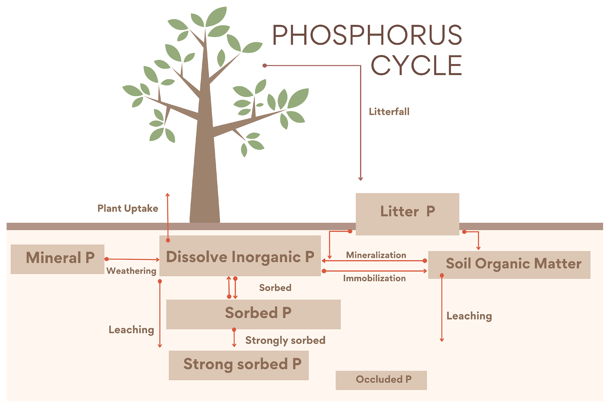
Figure 2 Diagram representing the UVic ESCM CNP P cycle. Weathering from mineral P is the only input into the soils. There are four inorganic pools (dissolved inorganic, adsorbed, strongly sorbed and occluded P) and three organic pools (vegetation (root, wood and leaf), litter and soil organic matter). As in Wang et al. (2010), the flux from strongly sorbed P to the occluded pool is not represented here; instead it is assumed to be a fraction of the total soil P.

2.3.1 Input

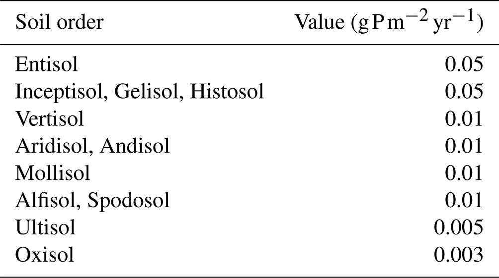
The P module estimates weathering input following Wang et al. (2010) and is driven by a fixed estimate (Table 3) of P release assigned by soil order divided into 12 classes from the US Department of Agriculture (USDA) soil order map.

Table 3 Constants for P input from Wang et al. (2010). The values change depending on the weathering state of the soil type. Highly weathered soils have lower values.

Additionally, an extra input structure was tested in the model but was not used for the P results in this study. It was implemented to compare the benefits of a static and a dynamic weathering scheme into the P pool. In this method weathering depends on runoff following Hartmann et al. (2014) using the lithological world map with 16 different classes generated by Hartmann and Moosdorf (2012). Equation (9) shows the estimation of the chemical weathering rate:

$$\begin{array}{}\text{(9)}& {\displaystyle }{F}_{\text{CW}}=b_{i}q,\text{(10)}& {\displaystyle }{b}_i=b_{\text{carbonate}}+b_{\text{silicate}},\end{array}$$

where F_CW ($\mathrm{t}{\mathrm{km}}^{-\mathrm{2}}{\mathrm{yr}}^{-\mathrm{1}}$) is the chemical weathering rate, q is the runoff (mm yr⁻¹) and b_i is the factor for each lithological class i; shielding correction functions were not applied. The chemical weathering is defined as the total fluvial export of Ca + Mg + K + SiO₂ and carbonate-derived CO₃; b_carbonate and b_silicate are chemical weathering parameters associated with carbonate and silicate rocks, respectively, found in Hartmann et al. (2014). Here we only apply the Wang et al. (2010) approach, as we found it to be more controllable and advantageous for the planned coupling of the P flux from land into the ocean. Hartmann et al. (2014) requires the estimation of runoff by the model structure. Hence, while representing a dynamical P release, it needs to be carefully assessed so that no extreme overestimation or underestimation is represented regionally. The Wang et al. (2010) approach provides constant input without variability, which in this particular case is favourable.

2.3.2 Inorganic soil phosphorus

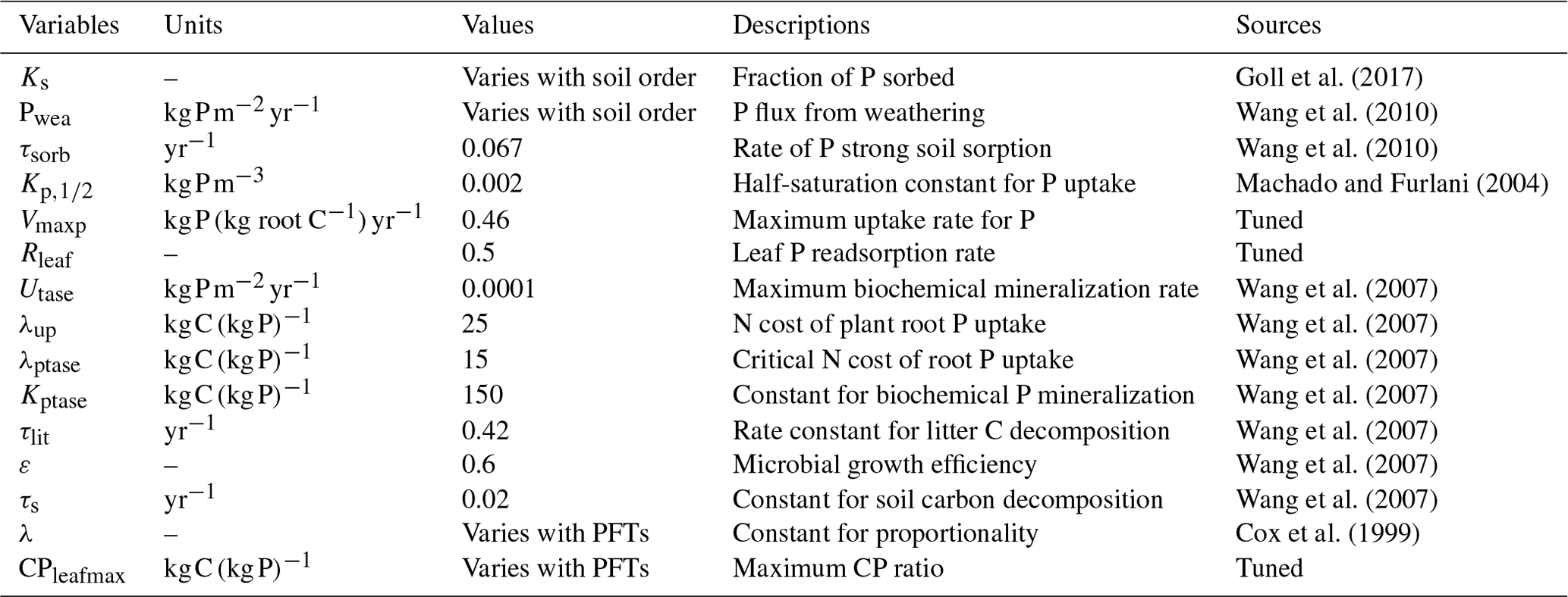
Inorganic P (P_soil) in soil follows the dynamics described in Goll et al. (2017) in Eq. (11), where each time step of a fixed fraction (k_s) of P is adsorbed, and the rest is dissolved (1−k_s). This fraction is based on the Hedley fractionation method (Hedley and Stewart, 1982), which is dependent on soil orders. The dataset has commonly been used to assess the different P forms in soil. The adsorbed P is regulated by k_s in Eq. (12) as determined by the soil order in the Hedley dataset:

$$\begin{array}{}\text{(11)}& {\displaystyle }\begin{array}{rl}{\displaystyle \frac{\mathrm{d}{\mathrm{P}}_{\text{soil}}}{\mathrm{d}t}}=& (\mathrm{1}-K_{\mathrm{s}})({\mathrm{P}}_{\text{wea}}+{\mathrm{P}}_{\text{litmin}}+{\mathrm{P}}_{\text{orgmin}}-{\mathrm{P}}_{\text{leach}}\\ & -{\mathrm{P}}_{\text{up}}-{\mathit{\tau }}_{\text{sorb}}{\mathrm{P}}_{\text{sorb}}-{\mathrm{P}}_{\text{imm}}),\end{array}\text{(12)}& {\displaystyle \frac{\mathrm{d}{\mathrm{P}}_{\text{sorb}}}{\mathrm{d}t}}=K_{\mathrm{s}}{\displaystyle \frac{\mathrm{d}{\mathrm{P}}_{\text{soil}}}{\mathrm{d}t}},\end{array}$$

where P_wea is the P released by rock weathering, P_litmin is the P mineralized from the P litter pool, P_orgmin is the P mineralized from the soil organic P, P_leach is the leached inorganic P, P_up is the P uptake by plants, P_sorb is the amount of P sorbed, τ_sorb is the rate of strong sorption and P_imm is the P immobilized from the inorganic P pool. The estimation of P_soil based on Goll et al. (2017) is originally taken from Goll et al. (2012). Here, the sum of P_sorb and P_soil constitutes the inorganic P pool in soil. Hence, the loss given by the rate of strong sorption is applied to the total inorganic P pool. The estimation of occluded P followed the Wang et al. (2010) approach, and based on Cross and Schlesinger (1995) the pool was assumed to be 35 % of the total soil P. P_leach and P_up were determined as in Eqs. (13) and (14) based on an adaptation of Wania et al.'s (2012) representation of leaching and uptake of N in the new soil layer model version:

$$\begin{array}{}\text{(13)}& {\displaystyle }{\mathrm{P}}_{\text{leach}}=Q_{\mathrm{D}}{\mathrm{P}}_{\text{soil}},\text{(14)}& {\displaystyle }{\mathrm{P}}_{\text{UP}}=\sum _{\text{PFT}}\left({\displaystyle \frac{V_{\text{maxp}}{\mathrm{C}}_{\text{root}}\left[{\mathrm{P}}_{\text{soil}}\right]F_{\text{root}}}{K_{\mathrm{p},\mathrm{1}/\mathrm{2}}+\left[{\mathrm{P}}_{\text{soil}}\right]}}\right),\end{array}$$

where Q_D is the runoff. V_maxp is the P maximum uptake rate, $K_{\mathrm{p},\mathrm{1}/\mathrm{2}}$ is the half-saturation constant for P, C_root is the root carbon and F_root is the root fraction.

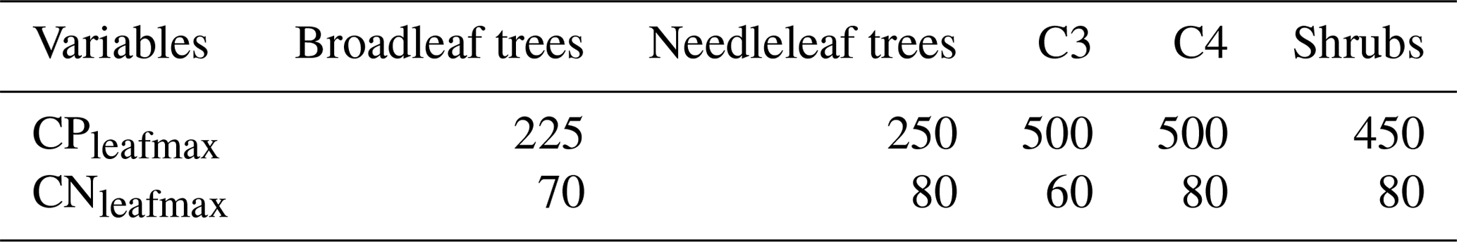
Table 4 Maximum leaf C:P and C:N in the CNP simulation by PFTs.

2.3.3 Organic soil phosphorus

After uptake, P is distributed in three vegetation compartments: leaf, root and wood. Leaf and root have a dynamic value that varies between a minimum and a maximum, while wood has a fixed CP ratio. The vegetation P biomass dynamics are determined from the difference between the amount of uptake and the loss from litterfall as in Eq. (15), and the litterfall is estimated as the CP ratio of the original model litterfall as in Eq. (16):

$$\begin{array}{}\text{(15)}& {\displaystyle \frac{\mathrm{d}\mathrm{Vegp}}{\mathrm{d}t}}={\mathrm{P}}_{\text{UP}}-{\mathrm{P}}_{\text{LF}},\text{(16)}& {\displaystyle }{\mathrm{P}}_{\text{LF}}=\sum _{\text{PFT}}{\displaystyle \frac{{\mathrm{Lit}}_{\text{leaf}}}{{\mathrm{CP}}_{\text{leaf}}}}(\mathrm{1}-R_{\text{leafp}})+{\displaystyle \frac{{\mathrm{Lit}}_{\text{root}}}{{\mathrm{CP}}_{\text{root}}}}+{\displaystyle \frac{{\mathrm{Lit}}_{\text{wood}}}{{\mathrm{CP}}_{\text{wood}}}},\end{array}$$

where V_egp is the vegetation P change over time; P_LF is the P litterfall; and Lit_leaf, Lit_root, and Lit_wood are the carbon litterfall rates for vegetation carbon. The leaf CP ratio is determined as

$$\begin{array}{}\text{(17)}& {\mathrm{CP}}_{\text{leaf}}={\displaystyle \frac{{\mathrm{C}}_{\text{leaf}}}{{\mathrm{P}}_{\text{leaf}}}},\end{array}$$

where C_leaf is the carbon content in leaves, and P_leaf is the P content in leaves. CP_leaf is one of the most important nutrient limiters in the model. The limiting effect of CP_leaf is when its value is higher than the maximum CP_leaf ratio parameter CP_leafmax. This leads to biomass reduction. In contrast to CN_leaf, CP_leaf does not control the maximum carboxylation rate of RubisCO. A more detailed description of nutrient limitation can be found in Sect. 2.4. The litter biomass is added to the P litter pool (P_lit), and its dynamic is based on Wang et al. (2007) as in Eq. (18):

$$\begin{array}{}\text{(18)}& {\displaystyle \frac{\mathrm{d}{\mathrm{P}}_{\text{Lit}}}{\mathrm{d}t}}={\mathrm{P}}_{\text{LF}}-{\mathit{\tau }}_{\text{lit}}{\mathrm{P}}_{\text{lit}}-{\mathrm{P}}_{\text{litmin}},\text{(19)}& {\displaystyle }{\mathrm{P}}_{\text{litmin}}={\displaystyle \frac{{\mathrm{P}}_{\text{lit}}}{{\mathrm{P}}_{\text{som}}+{\mathrm{P}}_{\text{lit}}}}{\mathrm{P}}_{\text{tase}},\text{(20)}& {\displaystyle }{\mathrm{P}}_{\text{tase}}=U_{\text{tase}}{\displaystyle \frac{{\mathit{\lambda }}_{\text{up}}-{\mathit{\lambda }}_{\text{Ptase}}}{{\mathit{\lambda }}_{\text{up}}-{\mathit{\lambda }}_{\text{Ptase}}+K_{\text{ptase}}}},\end{array}$$

where τ_lit is the rate constant for litter carbon decomposition (0.42 yr⁻¹), P_litmin is the biochemical P litter mineralization, P_tase is the biochemical P mineralization rate, U_tase is the maximum rate of P biochemical mineralization, λ_up is the N plant root cost to uptake P, λ_Ptase is the critical value of the N cost of root P uptake above which phosphate production starts and K_ptase is the Michaelis–Menten constant for biochemical P mineralization. Here, the N cost refers to the N required for protein structures involved in the metabolization of P in plants. P_tase is a constant value.

The decomposed soil litter is transferred to the soil organic P pool (P_som); the dynamics of P_som are adapted from Wang et al. (2007) as in Eq. (21):

$$\begin{array}{}\text{(21)}& {\displaystyle \frac{\mathrm{d}{\mathrm{P}}_{\text{som}}}{\mathrm{d}t}}={\mathit{\tau }}_{\text{lit}}{\mathrm{P}}_{\text{lit}}\mathit{\epsilon }-{\mathit{\tau }}_{\mathrm{s}}{\mathrm{P}}_{\text{som}}-{\mathrm{P}}_{\text{orgmin}},\text{(22)}& {\displaystyle }{\mathrm{P}}_{\text{orgmin}}={\displaystyle \frac{{\mathrm{P}}_{\text{som}}}{{\mathrm{P}}_{\text{lit}}+{\mathrm{P}}_{\text{som}}}}{\mathrm{P}}_{\text{tase}},\end{array}$$

where the first term represents the litter P input, while the other two are the P_som decomposition and mineralization. ε is the microbial growth efficiency (0.6), τ_s is the rate constant for soil carbon decomposition and P_orgmin is the biochemical P mineralization. The immobilization is determined from the NP ratio of the N immobilization estimated by Wania et al. (2012).

2.4 Nitrogen and phosphorus limitation

The N cycle limits the terrestrial vegetation productivity in two distinct ways: it first limits the photosynthesis efficiency by controlling the maximum carboxylation rate of RubisCO (V_cmax). The RubisCO enzyme plays a crucial role in the photosynthesis biochemistry by catalysing the carboxylation reactions in the Calvin cycle and has been found to be linearly related to the N leaf content (Walker et al., 2014). The original equation for V_cmax takes into account a fixed N leaf (Cox et al., 1999); this is replaced by Wania et al. (2012) in the first N cycle using the calculated inverse average canopy leaf $\mathrm{C}/\mathrm{N}$ ratio (CN_invleaf). In this representation the plant productivity is reduced when CN_leaf increases. V_cmax is calculated as

$$\begin{array}{}\text{(23)}& V_{\text{cmax}}=\mathit{\lambda }{\mathrm{CN}}_{\text{invleaf}},\end{array}$$

where λ is the constant of proportionality and 0.004 of C3 and 0.008 of C4 PFTs (Cox et al., 1999). Both N and P share the second form of limitation, where stoichiometric N and P limitation reduces the vegetation biomass. If the C:N ratio is too high, wood and root carbon biomass is transferred to the litter pool until the normal C:N ratio is reached (see Table 4).

The model assumes nutrient limitation when the estimated CN and CP leaf ratio is higher than the maximum CN (CN_leafmax) and CP (CP_leafmax) ratio in leaves. For grids with nutrient limitation the carbon in leaves is reduced to match the maximum CN or CP ratios in leaves. The carbon that is reduced is transferred to the litter pool. This reduction can happen for one or both nutrients until the ratio is met. The following equations regulate the reduction of biomass based on nutrient limitation:

$$\begin{array}{}\text{(24)}& {\displaystyle }{\mathrm{C}}_{\text{leaflimitedn}}={\mathrm{N}}_{\text{leaf}}{\mathrm{CN}}_{\text{leafmax}},\text{(25)}& {\displaystyle }{\mathrm{C}}_{\text{leafdiffn}}={\mathrm{C}}_{\text{leaf}}-{\mathrm{C}}_{\text{leaflimitedn}},\text{(26)}& {\displaystyle }{\mathrm{C}}_{\text{leaflimitedp}}={\mathrm{N}}_{\text{leaf}}{\mathrm{CP}}_{\text{leafmax}},\text{(27)}& {\displaystyle }{\mathrm{C}}_{\text{leafdiffp}}={\mathrm{C}}_{\text{leaf}}-{\mathrm{C}}_{\text{leaflimitedp}},\end{array}$$

where C_leaflimitedn and C_leaflimitedp are the carbon concentrations in leaves if the system is considered to be limited. C_leafdiffn and C_leafdiffp are the carbons lost due to nutrient limitation, and their values are summed in the litterfall equation when the system is nutrient limited.

2.5 Model runs and validation

The three different terrestrial biogeochemical versions, C, CN and CNP, were run for a historical simulation from 1850 to 2020. The C version serves as a baseline run representing the original version of the UVic ESCM ver. 2.10 (Mengis et al., 2020), the CN version is the modified version of the Wania et al. (2012) N model and CNP is the newest coupled model that includes P. Historical simulations are forced with fossil CO₂ emissions, dynamically determined land use change emissions, non-CO₂ greenhouse gas (GHG), sulfate aerosol, volcanic anomaly and solar. Furthermore, 24 historical simulations were run to assess the model sensitivity of six key parameters (CP_leafmax, CN_leafmax, R_leafp, R_leafn, V_maxp, V_maxn) in N and P limitation over terrestrial vegetation. The parameters were perturbed by increasing and reducing their value by 10 % and 20 % individually. CP_leafmax and CN_leafmax are the maximum leaf CP or CN ratios, respectively. If the values of CP_leaf and CN_leaf are above these thresholds, the model will take the system to be nutrient limited by either P or N. R_leafn and R_leafp are parameters that represent the resorption of N and P in leaves. This partly controls the loss of N and P from vegetation to the litter pool. V_maxp and V_maxn are the P and N maximum uptake rates.

Table 5 Phosphorus cycle model pools and variables.

Goll et al. (2017)Wang et al. (2010)Wang et al. (2010)Machado and Furlani (2004)Wang et al. (2007)Wang et al. (2007)Wang et al. (2007)Wang et al. (2007)Wang et al. (2007)Wang et al. (2007)Wang et al. (2007)Cox et al. (1999)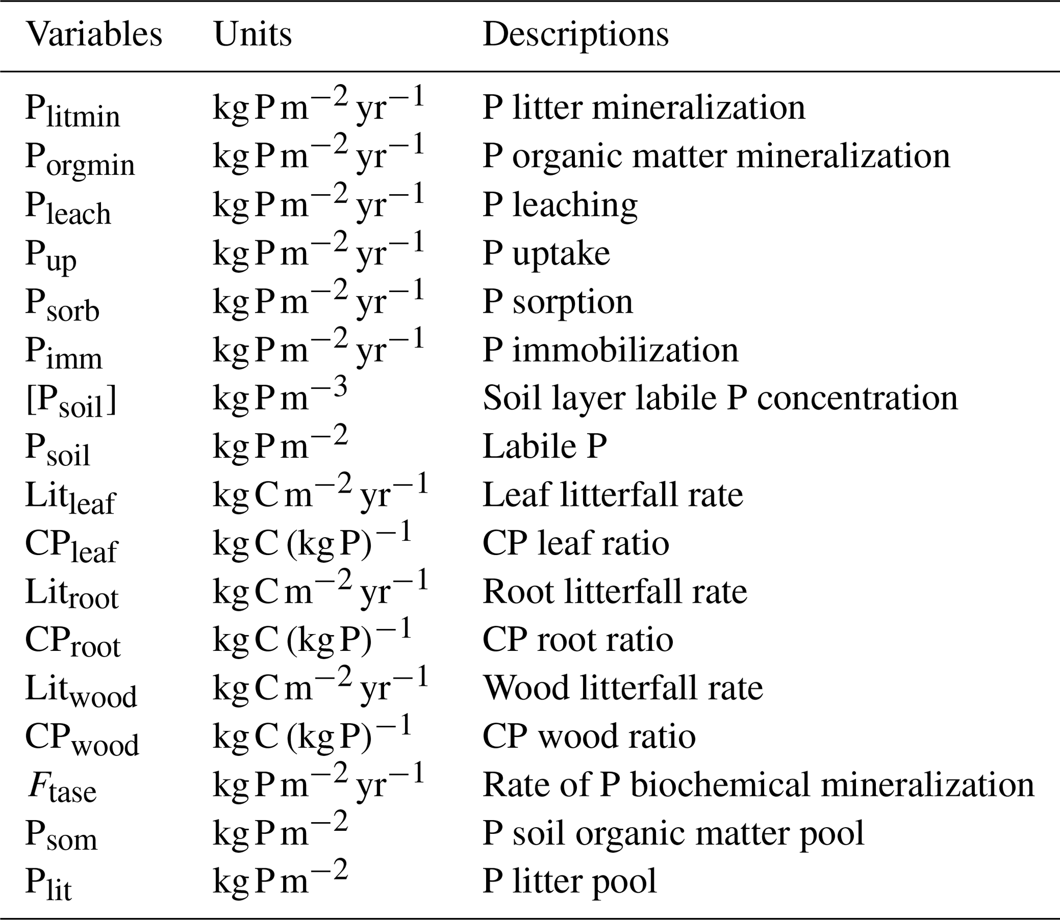

Table 6 Phosphorus cycle model parameters.

It should to be noted that the porting of the N cycle from version 2.9 to 2.10 of the UVic ESCM and later model spin-up could slightly alter the results presented in Mengis et al. (2020). Hence, our baseline model is slightly different from the standard UVic ESCM ver. 2.10. The N cycle is compared to Zaehle et al. (2010), Li et al. (2000), Yang et al. (2009) and Wania et al. (2012). The N₂O flux was compared with the Emissions Database for Global Atmospheric Research (EDGAR ver. 6.0; Crippa et al., 2021) dataset, which provided emission time series from 1970 until 2015 for non-CO₂ GHGs for all countries.

For the P cycle, we used as benchmark for the carbon cycle the UVic ESCM version 2.10 model calibration values and references, which included the Le Quere et al. (2018) datasets. The total soil P was calibrated with the He et al. (2021) dataset. The labile and sorbed pools were calibrated using the Yang et al. (2013) P distribution map dataset. For the use of the He et al. (2021) dataset we transformed the units with Eq. (28):

$$\begin{array}{}\text{(28)}& {\mathrm{P}}_{\text{soil}}={\mathrm{Bk}}_{\text{density}}\cdot {\mathrm{SL}}_{\mathrm{D}}\cdot {\mathrm{P}}_{\text{dataset}},\end{array}$$

where P_soil is the total P soil concentration (kg P m⁻²), Bk_density (kg m⁻³) is the bulk density taken from the International Geosphere–Biosphere Programme Data and Information System (IGBP-DIS) (Global Soil Data Task Group, 2014), SL_D (m) is the soil layer depth, and P_dataset (kg P (kg soil)⁻¹) is the He et al. (2021) dataset. The foliar stoichiometry was compared to the latitudinal trend from Reich and Oleksyn's (2004) N:P observations.

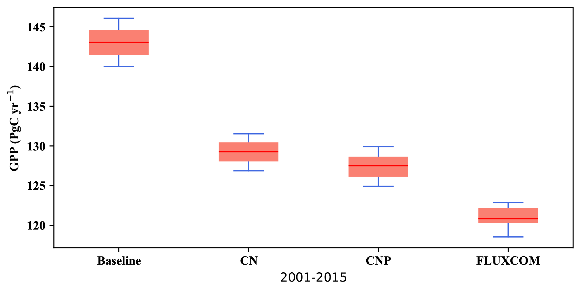
Figure 3 Modelled yearly gross primary productivity (GPP) from 2001 to 2015 versus the FLUXCOM GPP dataset (Jung et al., 2019).

One of the challenges of modelling nutrients in terrestrial systems is the lack of observations and validation datasets. Furthermore, the existing range of values for N and P variables is highly uncertain. This large range in values makes it difficult to accurately tune models. Although, improvements are in sight, with new artificial-intelligence-derived global datasets beginning to become available (He et al., 2021). Model validation has been advancing quickly in the last decade (Spafford and MacDougall, 2021) with tools such as the International Land Model Benchmarking (Collier et al., 2018) that significantly improve terrestrial model validation. However, there are limited variables available to compare to nutrient model development. The increase in the addition of nutrient structures in ESMs (Arora et al., 2020) suggests the need for terrestrial nutrient validation tools to improve model accuracy in the developmental phase. Moreover, a terrestrial nutrient model intercomparison project would unify global efforts to improve the representation of N and P in ESMs.

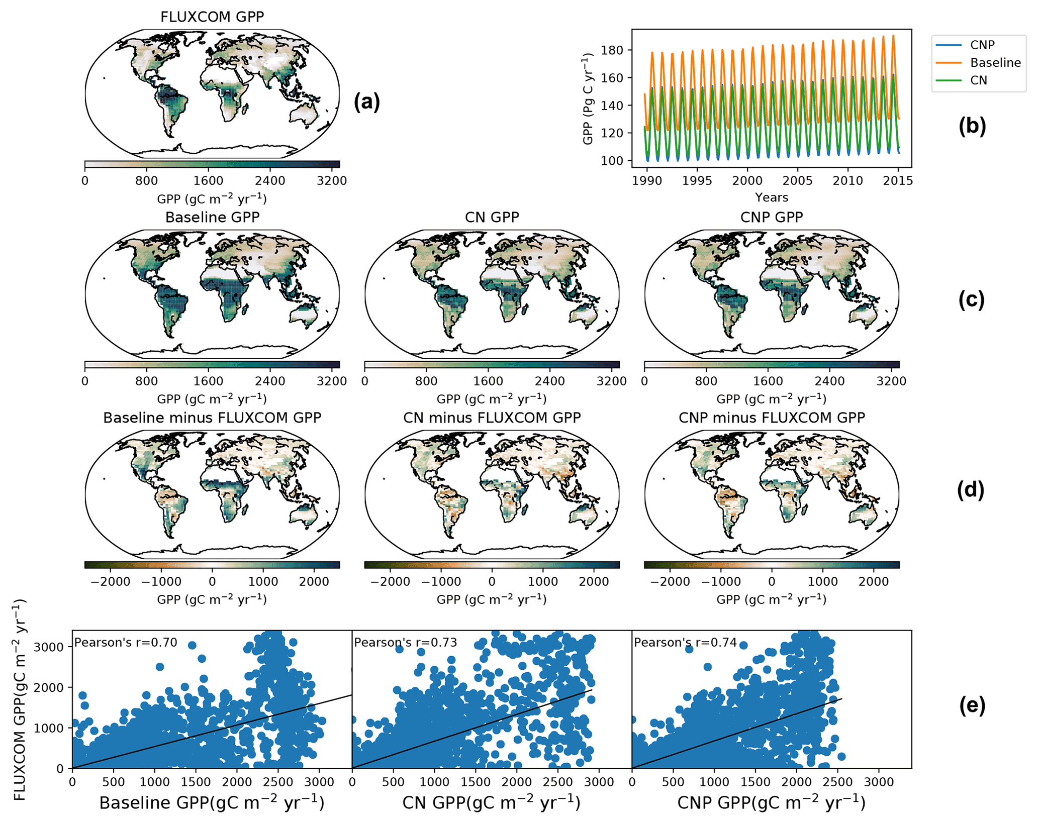
Figure 4 (a) The FLUXCOM GPP dataset from 2000–2010 and (b) seasonal GPP from 1990–2015 for the baseline, CN and CNP. (c) The second line shows the global GPP from 2000–2010 for the baseline, CN and CNP. (d) The third line shows the difference between the baseline, CN and CNP as well as the FLUXCOM GPP dataset. Panel (e) shows the correlation of the baseline, CN and CNP with the FLUXCOM GPP dataset.

3 Results and discussions

3.1 Carbon cycle

3.1.1 Land global primary productivity

The global gross productivity in CN and CNP resulted in a better agreement with the FLUXCOM GPP dataset (Jung et al., 2019) as shown in Fig. 3, with both CN and CNP overestimating the terrestrial global GPP average less than the baseline simulation. Compared to the baseline simulation (143 Pg yr⁻¹) both nutrient-limited model versions showed a reduced mean GPP from the years 2001–2015 with CN at 130 Pg yr⁻¹ and CNP at 127 Pg yr⁻¹. Furthermore, the modifications for the N cycle in regard to the mass balance changes resulted in the reduction in mean GPP from 129 Pg yr⁻¹ (Wania et al., 2012) to 122 Pg yr⁻¹ in the 1990s. The GPP distributions from the baseline, CN and CNP reproduce FLUXCOM dataset values reasonably well (Fig. 4). The seasonal pattern of GPP is also well represented within out simulations as shown in Fig. 4. The addition of nutrients improves the representation of GPP, where CNP had the highest correlation with the FLUXCOM GPP dataset. The high GPP in the baseline simulation can be explained by the overestimation of the vegetation biomass, especially broadleaf trees in tropical regions, as stated in Mengis et al. (2020). The representation of vegetation biomass is linked to the PFT fractions in the model. In the CN and CNP simulations the reduction in biomass is critical for the reduction in terrestrial productivity, especially in tropical regions where P availability has been shown to be a limiting factor for GPP (Du et al., 2020). Similarly to the findings of Wania et al. (2012), Bonan and Levis (2010), and Zaehle et al. (2010), the addition of nutrient limitation in ESMs seems to reduce GPP. Furthermore, locally in Amazonian soils, Nakhavali et al. (2022) found that the inclusion of P reduces the model GPP and NPP outputs by 5.1 % and 4.5 %, respectively, for a site simulation. Similarly to Nakhavali et al. (2022), we found an overall reduction in GPP in the Amazonian region.

The nutrient limitation reduced the amount of land–atmosphere carbon flux in the simulations. The cumulative land uptake from 1850–2005 was 150 Pg C yr⁻¹ in CNP, lower than the version 2.10 calibration in Mengis et al. (2020) (177 Pg C yr⁻¹). This change in response is crucial for understanding the future dynamics in the Shared Socioeconomic Pathway (SSP) projections, as terrestrial vegetation is expected to decrease its capacity to store carbon in the future (Goll et al., 2012). Overall, the carbon feedback values are in concordance with the ranges of the Global Carbon Project used in Mengis et al. (2020) (Le Quere et al., 2018) where the cumulative carbon flux was estimated to be 141 Pg C yr⁻¹ from 1850–2005. The atmosphere to land carbon flux follows the Global Carbon Project (GCP) dataset's (Le Quere et al., 2018) magnitude closely.

Similarly to Wania et al. (2012), we found higher values of NPP for CN (77.4 Pg C yr⁻¹) compared to the baseline simulation (74.2 Pg C yr⁻¹), while CNP (72 Pg C yr⁻¹) resulted in lower values due to the reduction in tropical vegetation biomass. CN and CNP results are close to the upper range (21.5 to 69.3 Pg C yr⁻¹) of simulated NPP shown in Li et al. (2015). The reduction in tropical biomass mainly in broadleaf tree carbon is reflected in the fraction of the PFT shown in the model output. Wania et al. (2012) argued that the reason behind the high NPP was the dependence of autotrophic respiration on N content in the leaf, root and stem, which are based on the original MOSES/TRIFFID version (Cox et al., 1999). In CN and CNP, the reduction in wood CN ratios and increase in N leaf content compared to baseline simulations, in which N leaf fluctuates from a minimum to a maximum value, gives place to the reduction in the maintenance respiration, which reduces the autotrophic respiration and consequently NPP. Furthermore, in the new CNP version, while wood CN remains fixed, the stoichiometrical reduction in wood carbon by the lack of P availability decreases wood carbon even more, especially in tropical forests and other tropical ecosystems.

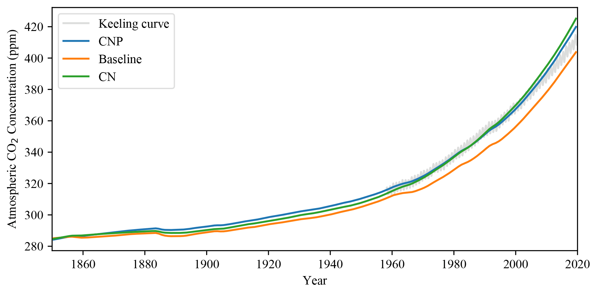
Figure 5 Atmospheric CO₂ concentration in CNP, CN and baseline simulations compared to the keeling curve from the Mauna Loa observatory (Keeling et al., 2005; grey line).

3.1.2 Atmospheric CO₂ concentration

The simulated CNP atmospheric CO₂ concentration matches observations very closely, and the addition of N and P has shown an improvement in the representation of the model accumulation of carbon in the atmosphere. The CO₂ concentration has improved compared to the evaluated 2.10 version of the UVic ESCM where from 1960 to 2010 the simulation deviated above the observed curve (Δ78 ppm in the simulation compared to Δ73 ppm observations; Mengis et al., 2020). Compared with the CN and baseline simulations (Fig. 3), CNP provides a more accurate representation of the atmospheric CO₂ concentration. Thus the nutrient limitation has effectively reduced the CO₂ fertilization effect on the terrestrial vegetation. Consequently, CN and CNP show a larger pool of atmospheric CO₂.

3.1.3 Terrestrial vegetation

Given that tropical forests and savannas are commonly limited by the availability of P, the simulated vegetation biomass representation is affected by the absence of nutrient limitation in ESMs. Nakhavali et al. (2022) found that the addition of P improved the vegetation estimations and the carbon cycle response to rising CO₂ for the Amazonian region, basing their study on a site representative of 60 % of the Amazonian soils.

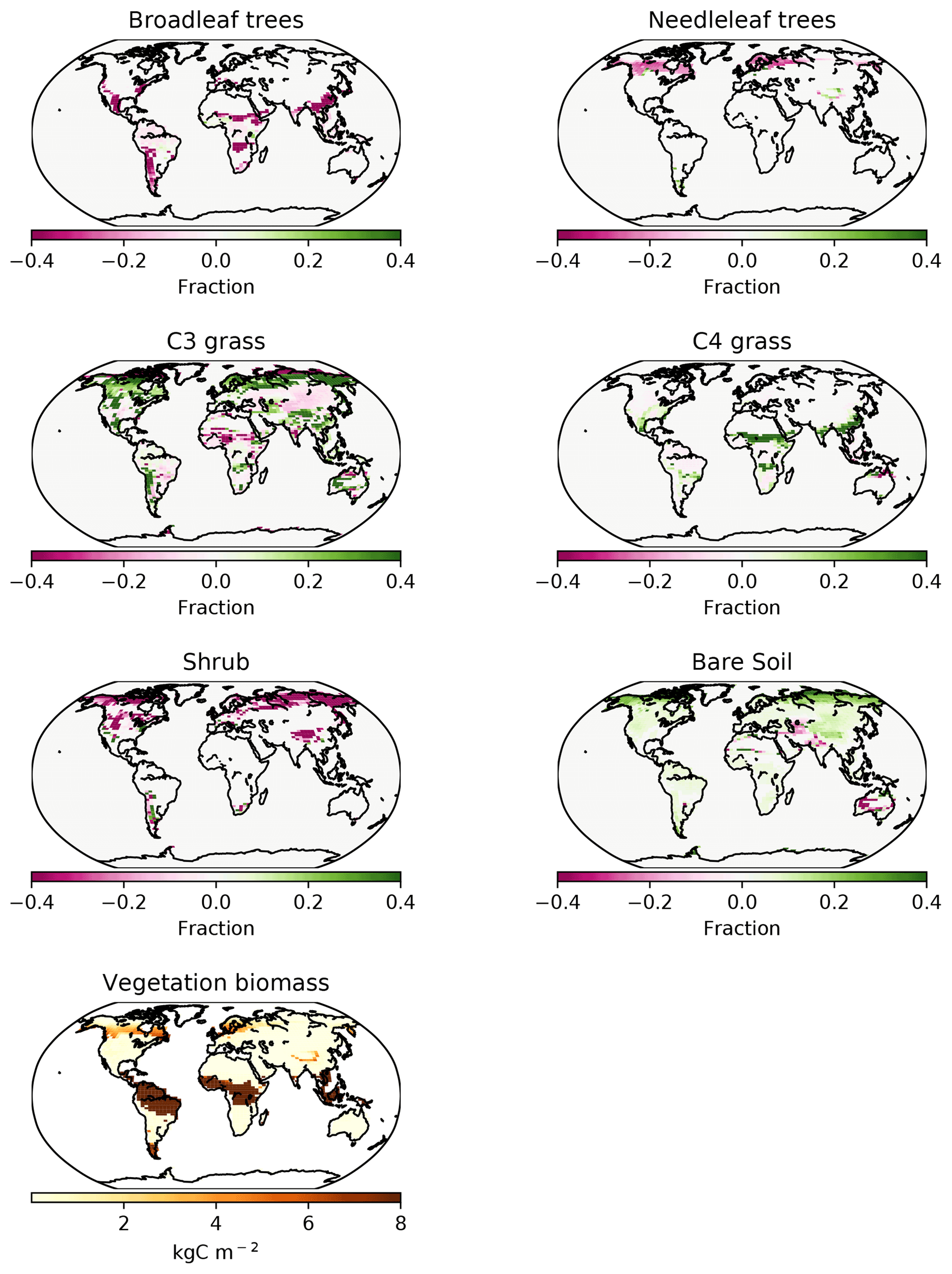
Figure 6 PFT fractions in the UVic ESCM for 1980–2010, CNP minus baseline. The last plot at the bottom shows CNP global biomass distribution.

In the CNP version of the model, broadleaf tree coverage declined in tropical and subtropical latitudes (Fig. 6) with the largest changes located in south eastern Asia, Africa and South America. The reduction in vegetation biomass ranged from 6 %–20 % in South America and Africa, while a higher reduction of 20 %–30 % was present in south eastern Asia. The magnitude of the continental difference can be attributed to the base internal vegetation biomass model version bias (Mengis et al., 2020). Additionally, CN and CNP show a shift in coverage where broadleaf trees are taken over by C3 grass.

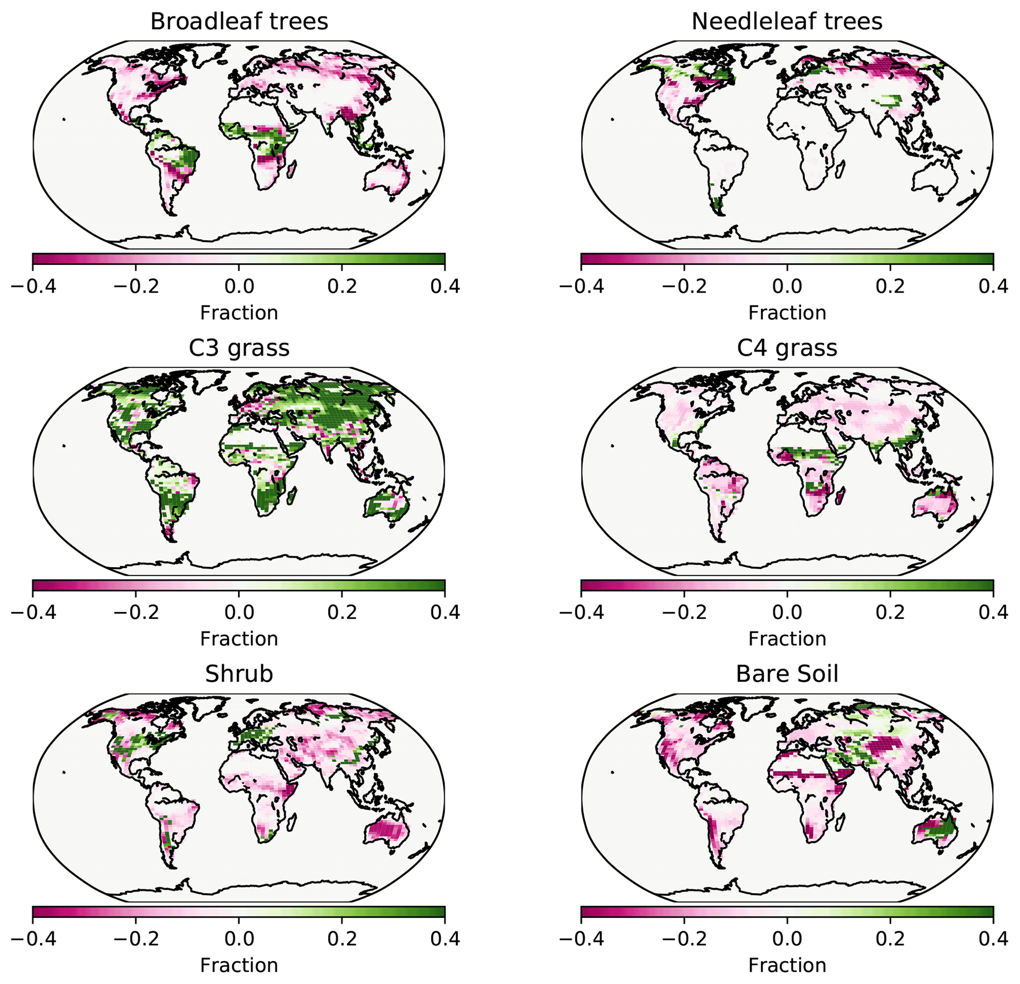
Figure 7 PFT fractions in the UVic ESCM for 2008–2012, CNP minus the Poulter et al. (2015) PFT dataset.

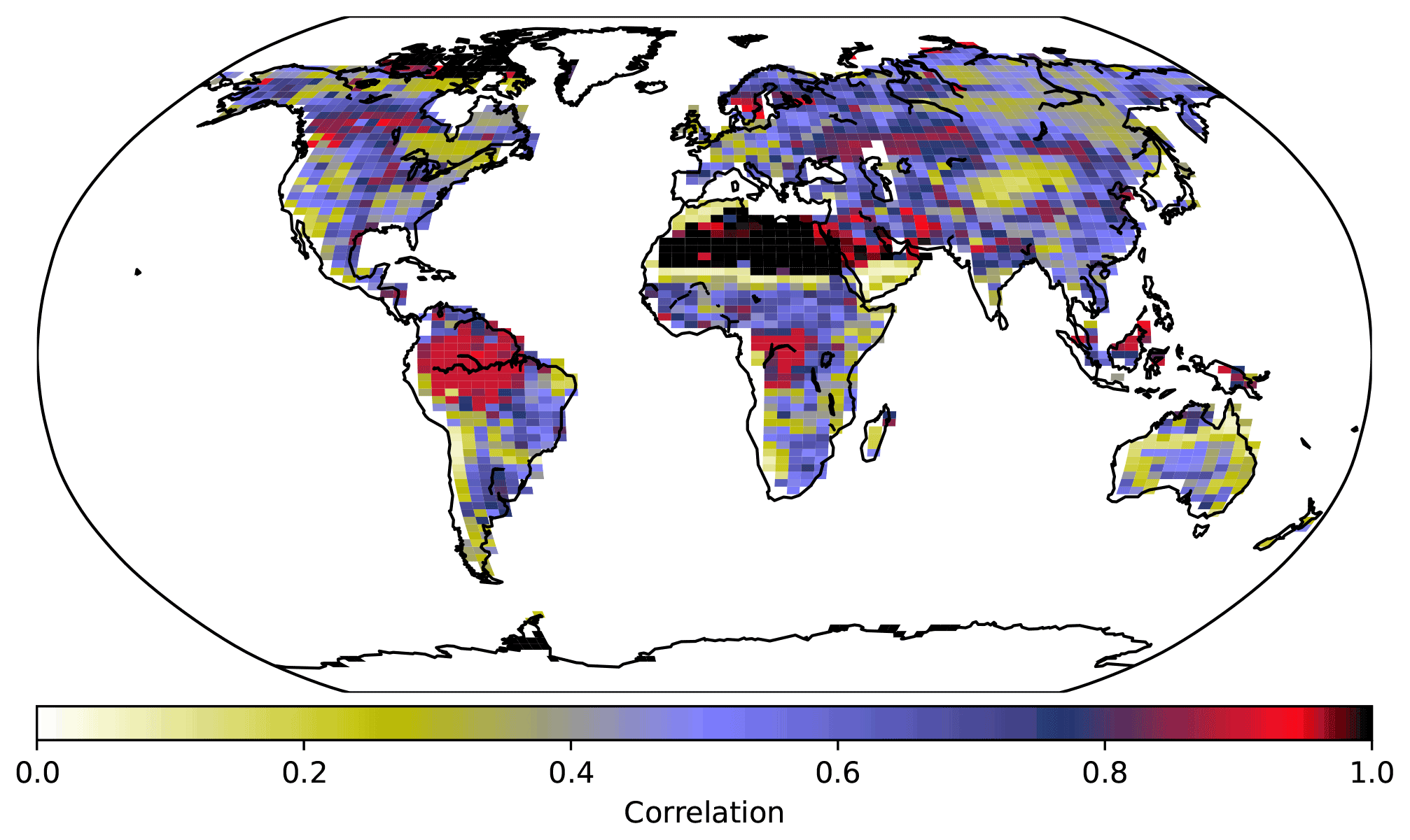
Figure 8 PFT fractions across grid cells in the UVic ESCM for 2008–2012, CNP correlation with the Poulter et al. (2015) PFT dataset.

Needleleaf trees were reduced in North America and Europe. Both CN and CNP simulations' vegetation carbon resulted in a decrease in vegetation biomass with 456 and 525 Pg C, respectively, compared to the baseline simulation (594 Pg C), similar to Zaehle et al. (2010). Overall CNP shows a high correlation with all PFT coverage when compared with the Poulter et al. (2015) PFT dataset. In tropical regions our model seems to represent vegetation closely to the data (Figs. 7 and 8).

The total vegetation carbon is similar to Wania et al. (2012), with tropical forests having a range from 8–16 and 4–12 kg C m⁻² in temperate and boreal forests with means of 10.50 and 6.7 kg C m⁻², respectively, compared to 12–16 and 4–12 kg C m⁻² and means of 13.4 and 7.3 kg C m⁻². The latitudinal mean shows a decrease in the range of vegetation carbon in tropical latitudes of 1–1.5 and 0.4–0.8 kg C m⁻² in northern template latitudes. These results indicate that the main reduction in vegetation carbon is in the tropics, which agrees with the general N and P global pattern (Du et al., 2020). Consistent with Wania et al. (2012), the vegetation carbon outputs are similar to those of Malhi et al. (1999), with 12.1 kg C m⁻² for tropical and 5.7–6.4 for temperate and boreal forests.

3.2 Nitrogen cycle

3.2.1 Nitrogen distribution

The soil N ranges from 0 to 1.5 kg N m⁻² with lower N in the tropics and increasing N towards the temperate regions. Globally, the CNP-simulated soil N is reduced compared to the original N structure in the UVic ESCM version 2.9 presented by Wania et al. (2012). The primary differences between the Wania et al. (2012) N cycle and the current version are the soil layer structure and the stoichiometry response to N limitation. In the former, N could be transferred from other pools when N was outside of the ratio threshold and thereby could be considered to be limiting vegetation.

This result is also lower than the 0 to 4.8 kg N m⁻² from the IGBP-DIS database (Global Soil Data Task Group, 2000). Wania et al. (2012) stated that the N content in the model is dependent on soil carbon fixed via a fixed CN ratio. Given this, lower carbon values can lower soil N values in CN simulations. Thereby, lower carbon in soil could be a strong reason why our results have less N than the IGBP-DIS database (Global Soil Data Task Group, 2000) and Wania et al. (2012). However, our values fall within the range of uncertainty. Our model estimates a mean BNF for 2010–2020 of 119 Tg N yr⁻¹. This value is above 35 Tg N yr⁻¹ from Braghiere et al. (2022) and within the range of 52–130 Tg N yr⁻¹ presented by Davies-Barnard and Friedlingstein (2020).

3.2.2 Vegetation nitrogen

The total amount of vegetation N (2.20 Pg N) was lower than the previous N cycle (2.94 Pg N, Wania et al., 2012). These values are similar to Zaehle et al. (2010) (3.8 Pg N) and Wang et al. (2018) (3.9 PgN) but lower than Li et al. (2000) (16 Pg N) and Yang et al. (2009) (18 Pg N). Our tropical (30 to 45 g N m⁻²) and boreal forest vegetation N (20 to 35 g N m⁻²) results are lower than the results from Wania et al. (2012) (30 to 40 g N m⁻²) and those of Xu-ri and Prentice (2008) and Yang et al. (2009) (both studies ranged between 150 and 400 g N m⁻²).

The global pattern of the CN ratio is similar to the Wania et al. (2012) structure with the highest located in tropical regions, especially South America and south eastern Asia. Tropical forests show a value that ranges from 230–280 C:N (Fig. 9) compared to 250–300 C:N shown by Wania et al. (2012). The reduction in wood carbon in the tropics by P limitation in CNP lowered the C:N ratios. Our values are within the observational range of uncertainty (95–730) stated in Martius (1992).

The distribution of vegetation N resembles the results of Du et al. (2020) where N's primary effect is in higher latitudes. The PFT fraction changes show that N mainly limits North and central America (BR and NL), Chile (BR), the Argentinian Patagonia (BR), northern Europe (NL), and eastern Asia (BR) (Fig. 6). However, there seems to be N limitation in tropical Africa and Asia in our model simulations. Even though our model does not represent co-limitation, the stoichiometric limitation does seem to indirectly capture this effect.

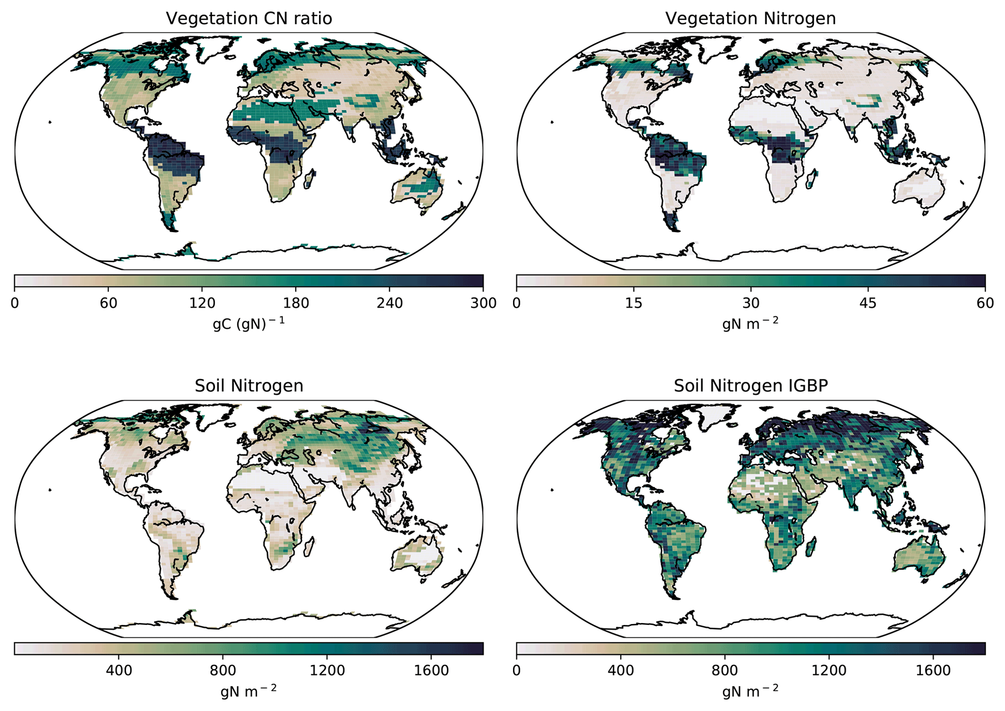
Figure 9 Modelled global soil and vegetation N in the CNP version of the UVic ESCM from 1980–1999. The lower-right map corresponds to the soil N from the IGBP-DIS dataset (Global Soil Data Task Group, 2000).

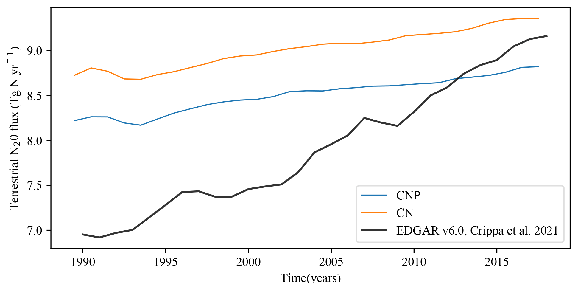
Figure 10 The CNP and CN global soil N₂O emissions vs. the EDGAR version 6.0 N₂O dataset (Crippa et al., 2021).

3.2.3 N₂O fluxes

The multilayer model has allowed for the estimation of anoxic regions, and, hence, a major improvement in the model is the quantification of terrestrial N₂O flux. Figure 10 shows CN and CNP N₂O fluxes from 1990 to 2018. Compared to the EDGAR version 6 dataset (Crippa et al., 2021), our model simulates N₂O fluxes relatively well, agreeing mostly in the last 10 years of the values. However, we observed an overestimation from 1990 to 2010. The CN version of the model fits within the lower natural (natural soil, atmospheric N deposition on land) and anthropogenic (agriculture, fossil fuel and industry) emission range (8.9–14.3 Tg N yr⁻¹) given by the Global Carbon Project (Tian, 2020), while CNP falls just below the lower-range value. The reduction in N in the model system by the P effect is shown by these results; the reduction in vegetation biomass and then litterfall reduces the amount of N transfer to the N soil pool, limiting the natural denitrification. The lack of oceanic production of N₂O in the model makes the comparison with the global total N₂O flux impossible at the moment. The total estimates for N₂O emissions are 4.2 to 11.4 Tg N yr⁻¹ for anthropogenic and 8.0 to 12.0 Tg N yr⁻¹ for natural emissions, as given by the Global Carbon Project (Tian, 2020). Assuming an ocean output of a mid-range emission (3.4 Tg N yr⁻¹), the model simulations are close to the lower range of the emission reported with CN (13.3 Tg N yr⁻¹) and CNP (12.1 Tg N yr⁻¹). Lighting and atmospheric production, biomass burning (addition of N₂O to atmospheric pool), and post-deforestation pulse effects are not taken into account in the model structure, and that could improve the fit of the simulation to a mid-range-level value.

3.3 Phosphorus cycle

3.3.1 Inputs and losses

The P global weathering rate estimated is 3 Tg P yr⁻¹, similar to 2 Tg P yr⁻¹ in Wang et al. (2010). Fertilization inputs of 1 Tg P yr⁻¹ (Filipelli, 2002) were added as an option to the model but were not used for the current simulations, and dust deposition is not accounted for. Hence, the only P input into the system in this experimental setup comes from rock weathering. Regarding the P weathering representation, the Hartmann et al. (2014) approach was tested at first, but the Wang et al. (2010) weathering scheme resulted in a better, simplified and controllable input. Although, the Hartmann et al. (2014) approach was found to be superior since P input is dynamic, incorporating model runoff and lithological map distribution. A dynamic P input will also require a better representation of P losses in order to maintain a steady state.

The P weathering was set so that the loss by leaching (3 Tg P yr⁻¹) was comparable to the riverine input stated in Filipelli (2002) of 4–6 Tg P yr⁻¹. The gap corresponds to anthropogenic inputs not included here. The preindustrial P input to the ocean from riverine input is 2–3 Tg P yr⁻¹, and human activities, especially agriculture (fertilizers) and water waste, roughly correspond to a doubling of the P input.

3.3.2 Land P pools and storages

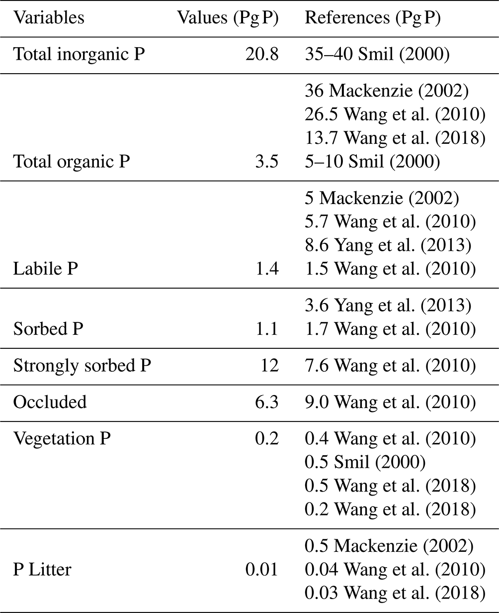
The total inorganic and organic P values are similar to those shown in the results of Smil (2000), Mackenzie (2002) and Wang et al. (2010) (Table 7), although organic P is slightly underestimated in the model (3.5 Pg P). This underestimation is likely the result of the lack of P fertilization on land. The labile P, sorbed P, strongly sorbed P and occluded pools are values comparable to Wang et al. (2010).

Smil (2000)Mackenzie (2002)Wang et al. (2010)Wang et al. (2018)Smil (2000)Mackenzie (2002)Wang et al. (2010)Yang et al. (2013)Wang et al. (2010)Yang et al. (2013)Wang et al. (2010)Wang et al. (2010)Wang et al. (2010)Wang et al. (2010)Smil (2000)Wang et al. (2018)Wang et al. (2018)Mackenzie (2002)Wang et al. (2010)Wang et al. (2018)

Table 7 Phosphorus cycle model pools and values for literature.

Figure 11 Soil and vegetation P global distribution. Modelled total P in soil, total P in soil as in He et al. (2021), soil P, labile P, vegetation biomass and the difference between modelled and observational P from He et al. (2021).

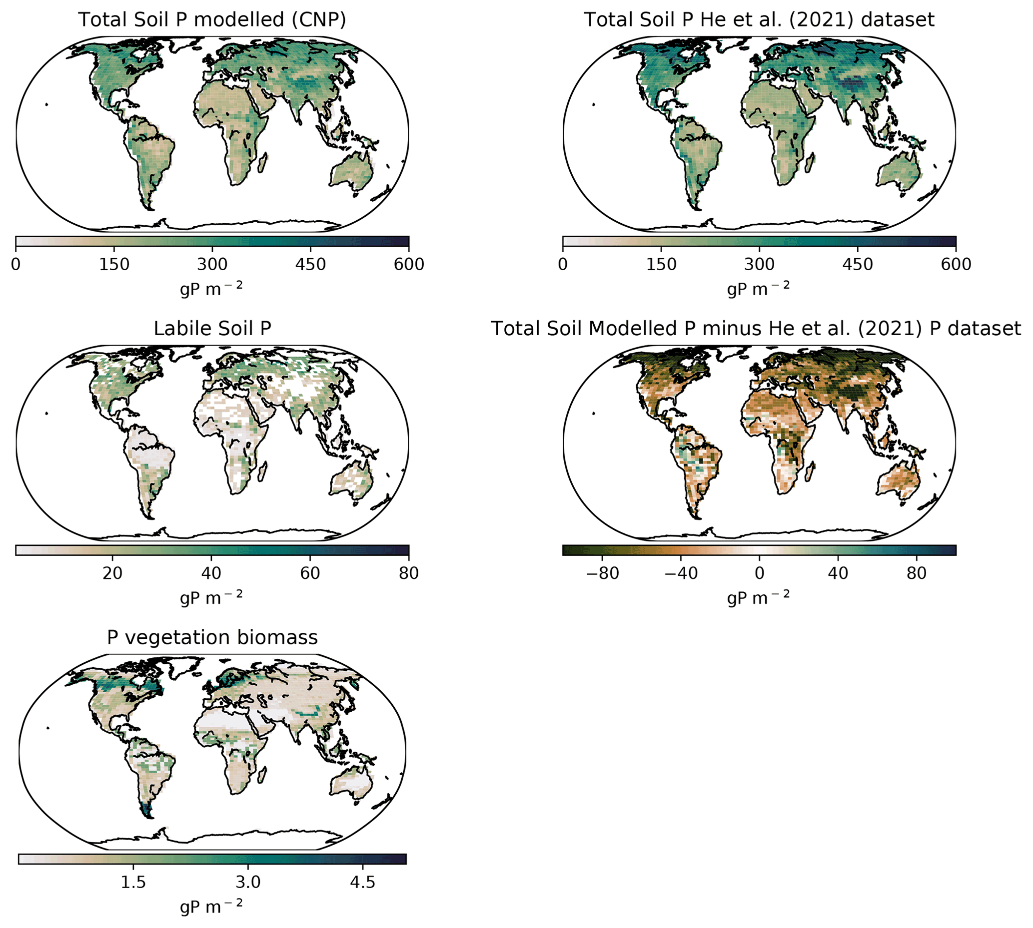
Globally the total soil P distribution (Fig. 11) is comparable to the He et al. (2021) dataset, which is one of the few terrestrial P concentration maps available. Overall, the model simulates less global P, especially in northern latitudes, most likely due to the oversimplified weathering scheme that underestimated the inputs in higher latitudes.

Latitudinally, the tropical soils showed the lowest P with the exception of highlands and mountains, while P increased sequentially towards the northern latitudes as shown in He et al. (2021). The labile P shows a similar distribution as Yang et al. (2013) with tropical regions being relatively depleted compared to other regions due to the high adsorption and occlusion by the soils.

In contrast with N, P inputs are limited by the mineral (apatite) concentration and weathering rate rather than biologically fixed. Most of the P is retained by soils, leaving a small labile fraction for biological uptake. Because P mineral weathering and chemical recycling in the soils are so constraining, our linear model approach for adsorption based on Goll et al. (2017) might overestimate the impact of adsorption and occlusion in tropical soils. It is also worth noting that the biological impact on the adsorption–desorption dynamics is missing in most P modules in ESMs. The release of P from mineral grains can be enhanced by either the reduction in pH due to respiration or the direct addition of organic acids by plant roots (Schlesinger, 1997).

3.3.3 Phosphorus in vegetation

The terrestrial vegetation shows a slight underestimation in comparison with other models. The new stoichiometry limitation scheme of the model plays an important role in the vegetation biomass and could be the reason for the underestimated values, especially for tropical regions. However, the range of P in terrestrial vegetation is still uncertain, with several studies showing a range from 1.8–3.0 Pg P (Smil, 2000). Although Wang et al. (2010) have dismissed those values as overestimations given an overall N:P ratio of 10–20 g N g P⁻¹, 3 Pg P is simply too high to be met.

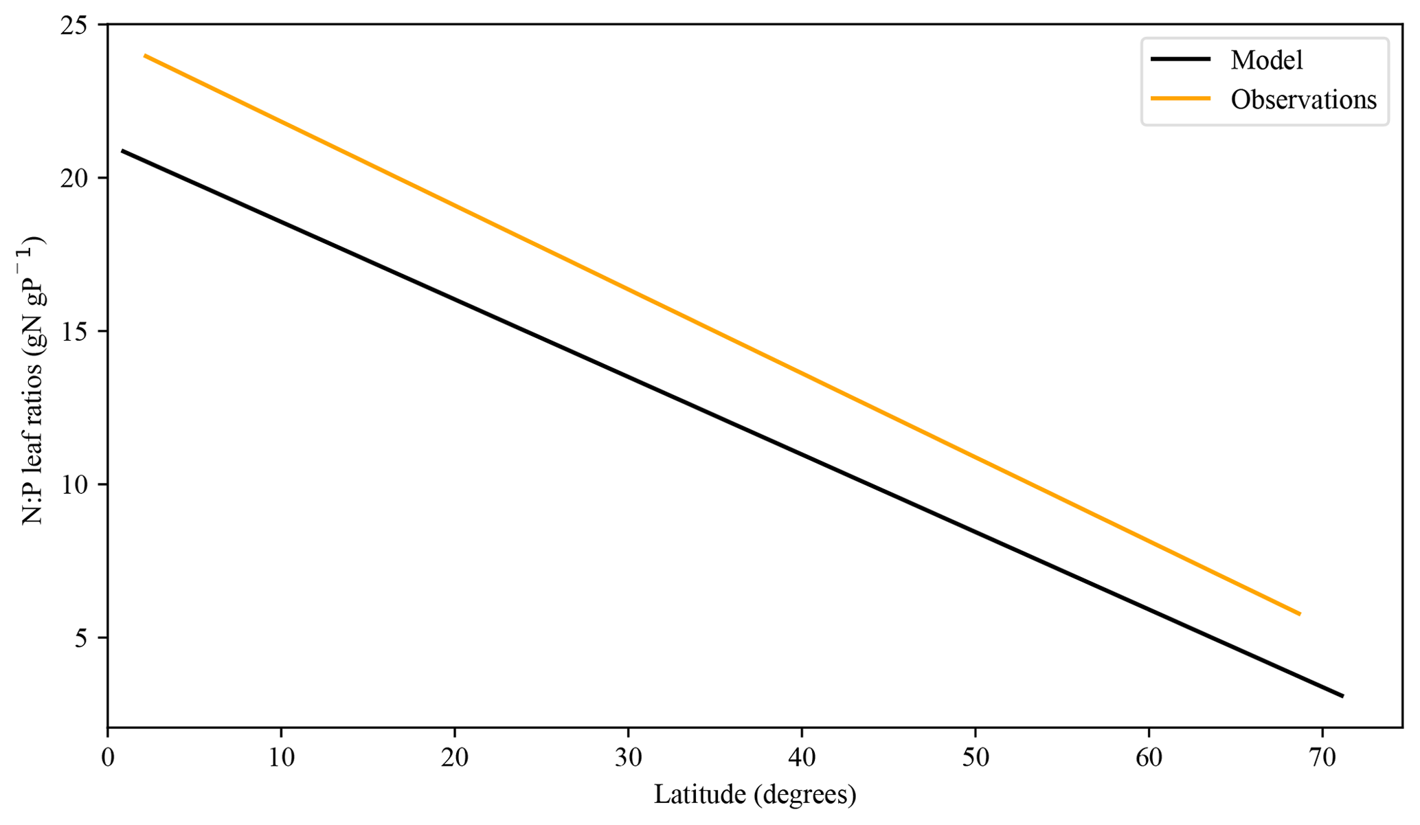
Figure 12 Modelled N:P leaf ratio trend vs. an empirical relationship derived from Reich and Oleksyn (2004).

The foliar stoichiometry seems to approximately follow the N:P ratio field measurements of Reich and Oleksyn (2004) (Fig. 12). The tropical regions show some underestimated values in our model; the low amount of labile P and the later decrease in broadleaf tree biomass could be responsible for the low numbers. Similarly, Nakhavali et al. (2022) show model values of 4–15 g P m⁻² for an Amazonian site, which surpasses our results.

A more complex adsorption–desorption scheme might be beneficial for solving the underestimation for tropical latitudes, as those regions are heavily sorbed and lose most of the input P, even though the need for a proper global P vegetation dataset is imperative to have proper ranges in global distributions. The mechanical reduction in vegetation stoichiometrically by the model structure might also be too simplistic to represent P limitation in the tropics.

3.4 Parameter sensitivity

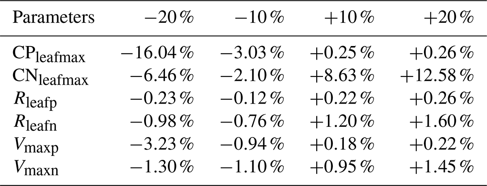
We perturbed six parameters (CP_leafmax, CN_leafmax, R_leafp, R_leafn, V_maxp, V_maxn) over historical simulations to assess the model sensitivity in terms of limitation of N and P. All of the above parameters play an important role in the nutrient limitation structure of the model. P_leafmax and N_leafmax control terrestrial vegetation when the stoichiometrical limitation is set to be enforced on terrestrial vegetation, and R_leafp, R_leafp, V_maxp and V_maxn control the uptake, litterfall and allocation of nutrients in leaves. In each case, default values were increased and decreased by 10 % and 20 % while holding other parameters constant. The results were compared to model simulations with all parameters held constant and set to default values. The cumulative atmosphere–land carbon flux was used to measure the effect of the perturbation, since the limitation directly affects this flux.

The results of the sensitivity study show that the model's sensitivity varies with different parameters (Table 8). The UVic ESCM is the most sensitive to perturbations of CP_leafmax and CN_leafmax because both directly determine the threshold by which vegetation carbon is reduced and nutrient limitation is defined. The model seems to be the most sensitive to changes in CP_leafmax. The regulation of this parameter is very useful for calibrating woody vegetation in tropical regions to improve the cover representation. The other parameters have a lower impact on the atmosphere–land carbon flux, ranging from −3.23 % to +1.60 %.

Table 8 Cumulative atmosphere–land carbon flux anomaly from the baseline (%). The parameters were perturbed by increasing and reducing 10 % and 20 % of their value.

4 Limitations and applications of the terrestrial nutrient modules

The UVic ESCM has been a critical tool in developing the cumulative emissions framework for climate mitigation (Zickfeld et al., 2009; Matthews et al., 2009; Matthews and Weaver, 2009; MacDougall and Knutti, 2016; Mengis et al., 2018; Tokarska et al., 2019). Due to its low computational cost and strict enforcement of matter and energy conservation, the model is capable of conducting a host of simulations beyond the limits of most other models but with higher resolution than other intermediate-complexity models (e.g. Montenegro et al., 2007; Matthews and Caldeira, 2008; Keller et al., 2014; MacDougall and Knutti, 2016; MacDougall, 2017; Pahlow et al., 2020; Kvale et al., 2021) . As terrestrial nutrient limitation constrains the carbon cycle in nature, the new N and P modules allow for addressing research questions relating to carbon budgets, carbon cycle and CH₄ feedbacks, carbon dioxide removal, and permafrost carbon cycles, among other questions. Furthermore, the N and P cycles can represent critical environmental and climate processes such as the release of N₂O, agricultural impacts on terrestrial soils and coastal lines, eutrophication, anoxic events, and nutrient fluxes from land to the ocean.

A number of limitations have been identified with the developed N and P modules that relate to the degree of complexity or the lack of large-scale datasets available. Due to the lack of global estimates of nutrient pools and fluxes based on field measurements, many of the parameters or parameterizations in this model are poorly constrained. In general, these are the following model limitations that are planned to be improved in future model development projects:

1. The model does not include a dynamic nutrient leaf resorption rate. Under nutrient limitations, this rate can increase as a strategy to conserve nutrients (Reed et al., 2012). Thus, the effect of limitation in our model might be overestimated.

2. There is a static input of P from weathering. To control the P input we chose to estimate weathering flux by adding a fixed amount. This oversimplification could add more uncertainty to the P pools and can be overcome using a runoff-based weathering scheme. Moreover, we do not account for P atmospheric dust deposition.

3. The sorption–desorption dynamics of P in soil are oversimplified. We chose the Goll et al. (2017) approach because it was a simpler way to represent this process. However, a more complex solution might improve the distribution of P globally.

4. An ocean N₂O output is absent. Consequently, we are unable to estimate the total amount of a dynamically evolving N₂O concentration at this time. As N₂O is the third most important greenhouse gas (IPCC, 2022), its incorporation into the model is a priority.

5. The model does not account for root uptake constrains of N and P on terrestrial vegetation. This includes spatial representations of mycorrhizal associations and the carbon cost of nitrogen and phosphorus uptake from soil (Shi et al., 2016; Braghiere et al., 2021, 2022).

The CNP model is primarily designed to improve carbon cycle feedbacks under current and future climate conditions. The use of nutrient limitation improves the land–atmosphere dynamics. In simulations, this improvement has a significant impact on atmospheric CO₂ concentrations. In future studies, we intend to assess the impact of nutrient limitation on different SSP scenarios and key carbon cycle benchmark metrics. Furthermore, the model can be used to improve the vegetation representation in ESMs. Finally, the CNP model may be used to generate coastal nutrient input and to integrate terrestrial nutrient biogeochemical processes with oceanic processes.

5 Conclusion

The N and P cycles simulated here fit into the range of uncertainty shown in datasets and other modelling efforts. Generally, our values fall into the lower range of the spectrum. N is limited in mainly high latitudes, especially in northern regions, but does show some limitation in tropical Africa and Asia. P limitations are greater in tropical regions and reduced the vegetation biomass compared to the carbon-only version of the model, bringing the model closer to observations (Mengis et al., 2020).

The two nutrient limitation models have improved the representation of the atmospheric carbon concentration in simulations forced with CO₂ emissions using the Keeling curve as benchmark data. The land–atmospheric flux fits other simulation datasets and has been reduced from Mengis et al.'s (2020) values. Overall N and P addition has improved the carbon cycle feedbacks simulated in historical simulations. The GPP is lowered, especially in the tropics, mainly due to the reduction in woody vegetation biomass.

Many improvements remain to be made in our model structure. In regard to the N cycle, denitrification processes need to be improved, and N₂O fluxes, while of the same magnitude as observations, lack the trend shown in other benchmark datasets. The complexity of the P cycle could be improved, especially the input and sorption processes. Finally both N and P cycles could gain accuracy from adding dynamic leaf reabsorption rates that have been shown to change when nutrient limitation is present in the ecosystem and that can be used as in Du et al. (2020) to clearly map the limitation pattern. Despite these limitations the improved model has shown higher fidelity to observations and is expected to improve projections of future key carbon cycle feedbacks.