the Creative Commons Attribution 4.0 License.
the Creative Commons Attribution 4.0 License.
 | 11 Jul 2023
An approach to refining the ground meteorological observation stations for improving PM2.5 forecasts in the Beijing–Tianjin–Hebei region
Lichao Yang
Wansuo Duan
Zifa Wang
This paper investigates how to refine the ground meteorological observation network to greatly improve the PM2.5 concentration forecasts by identifying sensitive areas for targeted observations that are associated with a total of 48 forecasts in eight heavy haze events during the years of 2016–2018 over the Beijing–Tianjin–Hebei (BTH) region. The conditional nonlinear optimal perturbation (CNOP) method is adopted to determine the sensitive area of the surface meteorological fields for each forecast, and a total of 48 CNOP-type errors are obtained including wind, temperature, and water vapor mixing ratio components. It is found that, although all the sensitive areas tend to locate within and/or around the BTH region, their specific distributions are dependent on the events and the start times of the forecasts. Based on these sensitive areas, the current ground meteorological stations within and around the BTH region are refined to form a cost-effective observation network, which makes the relevant PM2.5 forecasts starting from different initial times for varying events assimilate fewer observations, but overall, it achieve the forecasting skill comparable to and even higher than that obtained by assimilating all ground station observations. This network sheds light on the idea that some of the current ground stations within and around the BTH region are very useless for improving the PM2.5 forecasts in the BTH region and can be greatly scattered to avoid unnecessary work.
- Article
(13319 KB) - Full-text XML
- BibTeX
- EndNote


Air pollution has become a serious environmental issue in many Asian countries in recent decades. The Beijing–Tianjin–Hebei region (BTH region), being one of the most prosperous and populated regions in China, has suffered from successive heavy haze events during the past several decades (Xiao et al., 2020). Despite large reductions in primary pollutant emissions due to the recent strict pollution control policies in China, heavy haze events have still occurred in recent years, even during the COVID-19 lockdown period (Huang et al., 2021). Particulate matter with an aerodynamic diameter that is smaller than 2.5 (PM2.5) has dominated as one of the main air pollutants during the haze events. Exposure of a large population to high PM2.5 will pose a higher health risks and even a higher death rate (GBD 2017 Risk Factor Collaborators, 2018; World Health Organization, 2021). Therefore, an accurate prediction of the PM2.5 concentration is critical for providing early warnings to residents and helping governments take timely actions.
To accurately predict the PM2.5 concentrations, it is crucial to improve the quality of meteorological conditions and emissions, since chemical transport models (CTMs) require their information as input. Although the initial chemical concentrations and emission play important roles in air pollution forecasts, the meteorological conditions still substantially influence the PM2.5 variations at the regional scale (Liu et al., 2017; Lou et al., 2019; Chen et al., 2020). In terms of the effect of meteorological initial conditions, lots of studies have shown that small uncertainties in meteorological initial fields will result in large uncertainties in PM2.5 forecasts (Gilliam et al., 2015; Bei et al., 2017). Recently, it has been recognized that a bad meteorological initial condition may even affect the forecast of the accumulation or dissipation processes of the PM2.5 event and could result in a false alarm with respect to heavy haze events (Yang et al., 2022). Therefore, an accurate meteorological initial condition is also crucial for the regional PM2.5 forecasts, in addition to the initial chemical concentrations and emission.
Data assimilation has been recognized as being one of the most effective ways to improve the accuracy of initial conditions (Talagrand, 1997). High-quality meteorological initial fields could be obtained by assimilating the observations from an observation network for atmospheric conditions (Snyder, 1996). Among the various meteorological observation sources, the observations from the ground meteorological stations are often assimilated to predict the meteorology fields (Hu et al., 2019; Devers et al., 2020; Yao et al., 2021). Yang et al. (2022) studied the uncertainties in the meteorological initial fields with respect to PM2.5 forecasts and found that the meteorological forecasts in the BTH region are much more sensitive to the meteorological initial errors at the ground level with a lead time of 12 h. They emphasized that the initial conditions located at the ground level may play an important role in the meteorological forecasts over the BTH, which will further affect the regional PM2.5 forecasts, especially for the forecasts with a lead time of 12 h. In this sense, assimilating the observations from the ground meteorological stations could make an important contribution to the improvement in the PM2.5 forecasting skill, especially in the BTH region.
In the past few years, a high quantity of meteorological stations have been constructed around the world to study atmospheric motions and the weather and climate variabilities. In China alone, there were more than 2000 stations operated by the China Meteorological Administration (CMA) in the year of 2020, and the locations of the stations are generally selected based on the administrative district and resident populations (http://data.cma.cn/, last access: 28 June 2023). Even though a huge number of meteorological stations exist to provide observations, assimilating more observations may not necessarily lead to much higher forecast benefits (Li et al., 2010; Liu et al., 2021). Liu and Rabier (2002) used a simple 1-D framework and the computation of the analysis error covariance to show that increasing the observation density beyond a certain threshold value would yield little or no improvement in the accuracy of the analysis. In fact, previous studies have applied both simple and complicated numerical models to argue that additional observations may not result in a large improvement in the forecasting skill (Bengtsson and Gustavsson, 1972; Morss et al., 2001; Yang et al., 2014). Theoretically, in the area of strong sensitivity to the initial values of the forecasts, assimilating few observations may result in better forecasting skill; conversely, slight improvements or even poorer forecasting skill could be the result, even though a large number of observations is assimilated in the area of weak sensitivity, due to the additional errors induced by an imperfect assimilation procedure or the unsolved scales and processes in the model (Janjić et al., 2018; Zhang et al., 2019). Thus, even if we have sufficient meteorological observations, which should be used for the observations and how many observations should be preferentially assimilated to obtain a higher forecasting skill is still a key question. For the ground meteorological stations of concerned here, it is therefore essential to identify which ones provide the additional observations that dominantly enhance the improvement in the PM2.5 forecast level. One of the development targets proposed by the China Meteorological Administration during the 14th Five-Year Plan period is to arrange the meteorological observation network more reasonably and scientifically (https://www.cma.gov.cn/zfxxgk/gknr/ghjh/202112/t20211208_4295610.html, last access: 28 June 2023). The results could provide guidance to refine the existing ground meteorological observation networks and to improve the PM2.5 forecasts in the BTH region and avoid unnecessary work.
The dominant meteorological stations to be identified, as mentioned above, would provide the meteorological observations that will have the largest impact on the PM2.5 forecasts of the concerned region. This idea belongs to the new observational strategy of “targeted observation”, which is the idea that assimilating additional observations at the target time t1 in some key areas (i.e., sensitive areas), compared to doing it in other areas, may reduce the forecast errors in the concerned area (verification area) at a future time t2 (verification time; t1<t2) to a larger degree. It is obvious that the meteorological stations located in the sensitive areas would provide the meteorological observations that dominantly promote the PM2.5 forecasts of the concerned area (i.e., the verification area). Some approaches, such as the singular vector (SV; Palmer et al., 1998), adjoint sensitivities (Langland et al., 1999), and the ensemble transform Kalman filter (ETKF; Bishop et al., 2001; Majumdar et al., 2002), have been used to identify the sensitive areas for targeted observations. However, these approaches are developed under the assumption that the initial errors are linearly developed in the nonlinear model, which is not completely true in the real atmosphere (Toth and Kalnay, 1993; Mu and Wang, 2001). In this study, an advanced fully nonlinear method, conditional nonlinear optimal perturbation (CNOP; Mu et al., 2003), is applied to find the initial perturbation of the fastest growth in the nonlinear model and then to determine the meteorological sensitive area of the PM2.5 forecasts. It has been verified that the sensitive area identified by the CNOP shows advantages when compared with the areas identified by traditional methods through both the theoretical proof and numerical experiments (Qin and Mu, 2011; Chen et al., 2013; Duan et al., 2018; Feng et al., 2022; Qin et al., 2013). The CNOP has been adopted to identify the sensitive areas in the studies of tropical cyclones, El Niño–Southern Oscillation events, oceanic mesoscale eddies, and marine environments and has successfully improved the forecasting skill (see the review of Duan et al., 2023). Moreover, Yang et al. (2022) applied the CNOP to determine the sensitive areas for targeted observation of a heavy haze event of which authorities were not warned in time by the monitoring center and demonstrated that assimilating additional observations in such a sensitive area leads to the successful forecast of the PM2.5 concentrations with much higher skill. Then, in this study, we would use the CNOP to recognize the dominant ground meteorological stations applicable for PM2.5 forecasts by investigating the sensitive areas of eight winter heavy haze events over the BTH region during the years of 2016–2018, consequently providing an idea to refine the current ground meteorological stations for improving the PM2.5 forecasts in the BTH. It is noted that, during this period, as encouraged by the strict pollution control policies issued by the Chinese government, great efforts have been made to produce a more accurate high-resolution emission inventory (Zheng et al., 2020), which is favorable for better simulating the chemical components in China and then separating the meteorological uncertainty effects of interest in the present study.
The remainder of the paper is organized as follows. In Sect. 2, we introduce the model, data, and method. In Sect. 3, we reproduce the eight heavy haze events that occurred in the BTH during 2016–2018 and identify the sensitive areas of the surface meteorological conditions for the PM2.5 forecasts with the application of the CNOP method. Then a cost-effective meteorological observation network is constructed in Sect. 4, which has been verified to be an approximation of the whole BTH network of ground meteorological stations to improve the PM2.5 forecasts. In Sect. 5, we interpret the reasons why assimilating the cost-effective observations can lead to an improvement in the PM2.5 forecasting skill that is comparable to assimilating all ground observations from the perspectives of thermodynamics and dynamics, and in Sect. 6, a summary and discussion is provided.
In this study, we use the Weather Research and Forecasting Model (WRF) and its adjoint model, and the nested air quality prediction modeling system (NAQPMS), to identify the sensitive areas of surface meteorological conditions associated with the regional PM2.5 forecasts by the application of the CNOP approach.
2.1 Models
The NAQPMS model is a 3-D regional Eulerian chemical transport model, which contains emissions, advection/convection, diffusion, dry and wet deposition, and gas/aqueous chemical modules (Wang et al., 1997, 2006). It has been widely used in scientific studies and practical forecasts for air quality in China. The anthropogenic emissions are obtained from Multi-resolution Emission Inventory model for Climate and air pollution research (MEIC; http://meicmodel.org/, last access: 28 June 2023). Since we only focus on the sensitivity of the meteorological conditions for PM2.5 forecasts in the present paper, the emission inventory is assumed to be perfect and is kept the same in all of the simulations. The modeling domain includes 119×119 grids, with a horizontal resolution of 30 km and 20 levels in the vertical. The composition of the PM2.5 matter considered in the model includes black carbon, organic carbon, secondary inorganic aerosol (sulfate, nitrate, ammonium), and primary PM2.5 emitted directly from various sources.
The NAQPMS model is driven by the meteorological fields generated through the WRF (http://www.wrf-model.org/, last access: 28 June 2023). The parameterization schemes adopted in the WRF model include the Lin microphysics scheme (Lin et al., 1983), Dudhia shortwave radiation schemes (Dudhia, 1989), rapid radiative transfer model for global climate models (RRTMG) longwave radiation (Iacono et al., 2008), and Yonsei University planetary boundary layer parameterization scheme (Hong et al., 2006). The adjoint model of WRF also uses the same parameterization schemes. Both the WRF model and the adjoint model of WRF are configured with the same horizontal and vertical grid structure with the NAQPMS model.
2.2 Data
There are eight typical heavy haze events that occurred in the BTH region during the wintertime (OND or October–November–December) in the years of 2016–2018 (Table 1), and all eight events and their associated forecasts are investigated in the study. The observed surface PM2.5 concentration datasets of the events are obtained by the national environmental monitoring stations. In total, there are 80 air quality monitoring stations within the BTH region (see the geographical distribution for these 80 stations in Fig. 1a). From these stations, we retrieved the hourly PM2.5 concentration time series for each of the eight events.
Table 1The root mean square error (RMSE; µg m−3) and correlation coefficient (CC) of the PM2.5 concentrations between the simulations initialized by the ERA5 Global Forecast System (ERA5/GFS) and the observations in the eight heavy haze events. The simulation of a smaller RMSE and higher CC is marked in bold. Note that BJT is for Beijing time (UTC+8 h).
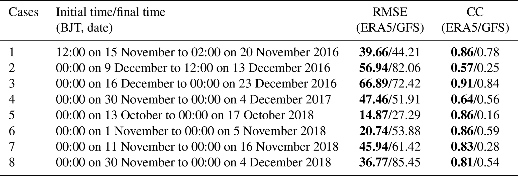
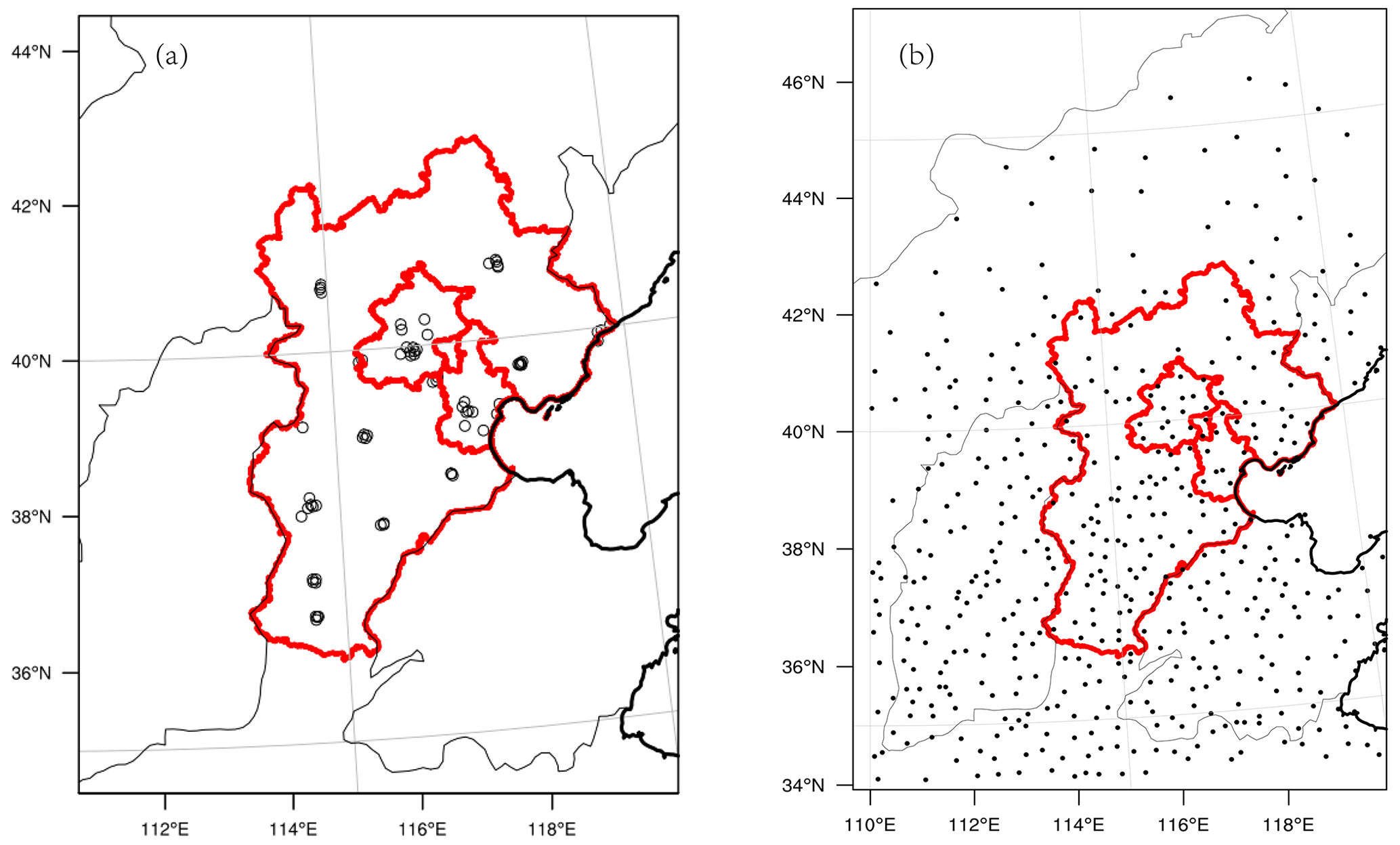
Figure 1The maps of (a) the 80 environmental monitoring stations (black circles) within the BTH region and (b) the 481 national ground meteorological stations (black dots) within and around the BTH region (34–46∘ N, 110–120∘ E). The black lines represent the boundaries of provinces in China, and the thick black lines are the coastline. The boundaries of Beijing city, Tianjin city, and Hebei province are the thick red lines.
To produce the initial and boundary conditions for WRF simulation, the fifth generation ECMWF reanalysis for the global climate and weather (ERA5; https://www.ecmwf.int/en/forecasts/datasets/reanalysis-datasets/era5, last access: 28 June 2023) and National Centers for Environmental Prediction Global Forecast System (NCEP GFS) historical archive forecast data (https://rda.ucar.edu/ datasets/ds084.1/, last access: 28 June 2023) are used.
2.3 Conditional nonlinear optimal perturbation (CNOP)
The CNOP represents the initial perturbation (or initial error) that results in the largest forecast error in the verification area at the verification time and is the most sensitive initial perturbation. The dynamical equation in the nonlinear model can be written as Eq. (1).
where t is the time, F is the nonlinear partial differential operator, and x is the state vector with an initial value x0. If we add an initial perturbation δx0 to the initial state x0, then the evolution of the two initial states at the prediction time T can be described as Eq. (2).
where M is the nonlinear propagator that propagates the initial value to the prediction time T. So δx(T) describes the evolution of the initial perturbation δx0 of the reference state x(T). An initial perturbation is called a CNOP () if, and only if,
The is the constraint condition of initial perturbation, and β is a positive value. C1 and C2 are coefficient matrices, which define the format of the initial perturbation and its evolution. Mathematically, the CNOP leads to the global maximum of the cost function under a certain constraint.
In our study, since we focused on the uncertainties in the meteorological initial condition associated with the PM2.5 forecast, following Yang et al. (2022), the state vector x consists of zonal and meridional wind (U and V, respectively), temperature (T), water vapor mixing ratio (Q), and pressure (P) components, which are considered to be important meteorological fields for PM2.5 forecasts over the BTH region (see the review paper of Chen et al., 2020). The perturbations δx0 are superimposed on the ground meteorological field x0 of interest. The amplitude of the initial perturbation and its evolution is defined by the total energy of the meteorological state at the ground level of the model domain and the integral of the total energy from ground to top (i.e., 100 hPa) at the verification areas (i.e., the BTH region), respectively. The expression of total energy is shown in Eq. (3) (Ehrendorfer et al., 1999).
where Cp (=1005.7 J kg−1 K−1), Ra (=287.04 J kg−1 K−1), Tr (=270 K), L ( J kg−1), and Pr (=1000 hPa) are constant values.
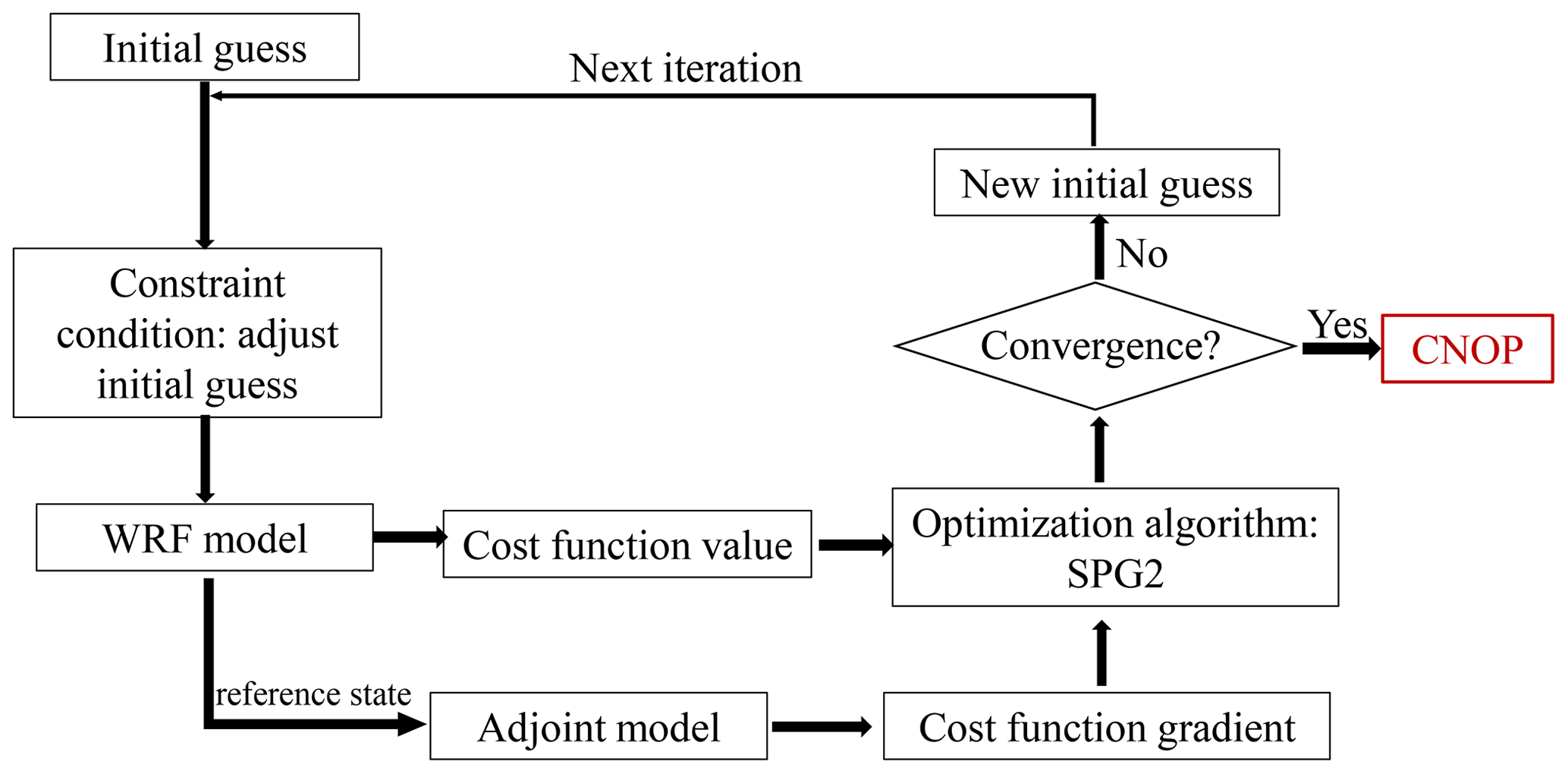
The spectral projected gradient 2 (SPG2) method is used to solve the optimization problem in Eq. (3). It is noted that the SPG2 algorithm is generally designed to solve the minimum value of a nonlinear function (cost function) with an initial constraint condition, and the gradient of the cost function with respect to the initial perturbation represents the descending direction in the search for the minimum cost function. Therefore, in this study, we have to rewrite the cost function in Eq. (3) as , and the WRF adjoint model is used to compute the gradient of the cost function. Specially, to calculate the CNOP, a first-guess initial perturbation, , is projected into the constraint condition and superimposed on the initial state x0 of the WRF model. After a forward integration of the WRF, the value of the cost function, i.e., , can be obtained. Then, with the adjoint model of the WRF, the gradient of the cost function with respect to the initial perturbation, ), is calculated. Theoretically, the gradient presents the fastest descending direction of the cost function. However, in realistic numerical experiments, the gradient presents a fast-descending direction that is not necessarily the fastest, so we need more iterations. After the iteratively forward and backward integrations of the WRF model governed by the SPG2 algorithm, the initial perturbation is optimized and updated until the convergence condition is satisfied, where the convergence condition is , and ε1 is an extremely small positive number. ) projects the initial perturbation to the constraint condition. Finally, the CNOP can be obtained. The flow chart of the CNOP calculation is shown in Fig. 2. For further details of the SPG2 algorithm, readers can refer to Birgin et al. (2001).
In this section, we first simulate the PM2.5 concentration variability using the WRF initialized by the ERA5 reanalysis data and NCEP-GFS forecast data separately to show the sensitivities of the PM2.5 forecasts to the meteorological initial uncertainties. Then we calculated the CNOP-type initial errors in the concerned forecasts and identify their sensitive areas.
3.1 Sensitivity to meteorological initial uncertainties in the PM2.5 variability simulations
For each of the eight heavy haze events, after the 10 d spin-up of WRF-NAQPMS, the ERA5 and the GFS data are separately used to initialize the WRF model, and then two forecasted meteorological fields can be obtained, which force the NAQPMS to output two kinds of simulations of PM2.5 concentrations. Table 1 provides the initial and final times of the eight event simulations, and Fig. 3 plots the two kinds of simulations of the PM2.5 concentrations averaged over the BTH region for each event and the corresponding observations. We take the event initialized at 00:00 BJT (Beijing time; UTC+8 h) on 30 November 2018 as an example to describe the difference between two kinds of simulations of the PM2.5 concentrations (see Fig. 4). Then, for this event, the ERA5 presents weak southerly winds with a mean speed of 1.06 m s−1 over the BTH region at the initial time, while the GFS shows stronger southerly winds with a speed of 1.91 m s−1. Obviously, the two simulations show a difference in the initial meteorological fields of this event. When the final time is reached after 18 h, the simulation initialized by ERA5 presents a weak northerly wind in the BTH region and forecasts a PM2.5 concentration of 93.05 µg m−3 on average over the BTH region; however, the simulation initialized by GFS enhances the southerly wind to 3.56 m s−1, and particularly in the southern part of Hebei, the southerly wind reaches 5.89 m s−1, which transports more PM2.5 from the south to the BTH region and results in the PM2.5 forecasts of 134.71 µg m−3 on average. It is noted that these two PM2.5 simulations are generated from the same emission inventory and the same initial chemical concentrations, with the initial PM2.5 concentration focused on the Anhui and Hubei provinces, which are located to the south of the BTH region. It is therefore certain that the difference between the two PM2.5 simulations of this illustrated event is only caused by the different meteorological initial fields. For other forecasts, it is also seen from Fig. 3 that different initial meteorological conditions result in different levels of accuracy in the PM2.5 simulation in terms of the magnitude, peak time, and even the variability in the accumulation and dissipation processes of the heavy haze event.
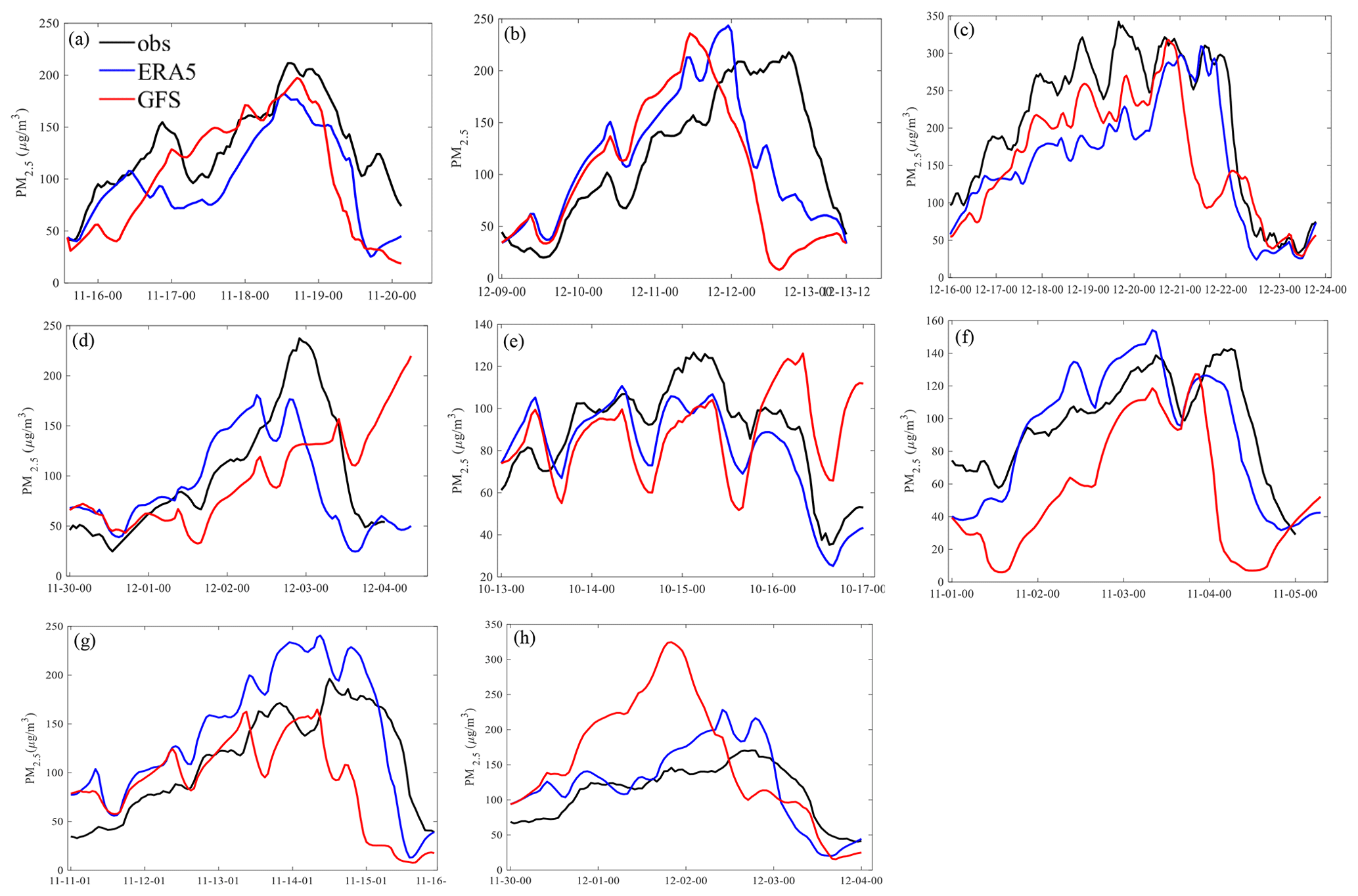
Figure 3Time series of the PM2.5 concentrations averaged over the BTH region of observations (black line) and simulations initialized by ERA5 (blue line) and GFS (red line) meteorological data during the eight heavy haze events in 2016–2018. These events occurred during the following times: (a) from 12:00 BJT on 15 November to 02:00 BJT on 20 November 2016, (b) from 00:00 BJT on 9 December to 12:00 BJT on 13 December 2016, (c) from 00:00 BJT on 16 December to 00:00 BJT on 23 December 2016, (d) from 00:00 BJT on 30 November to 00:00 BJT on 4 December 2017, (e) from 00:00 BJT on 13 October to 00:00 BJT on 17 October 2018, (f) from 00:00 BJT on 1 November to 00:00 BJT on 5 November 2018, (g) from 00:00 BJT on 11 November to 00:00 BJT on 16 November 2018, and (h) from 00:00 BJT on 30 November to 00:00 BJT on 4 December 2018.
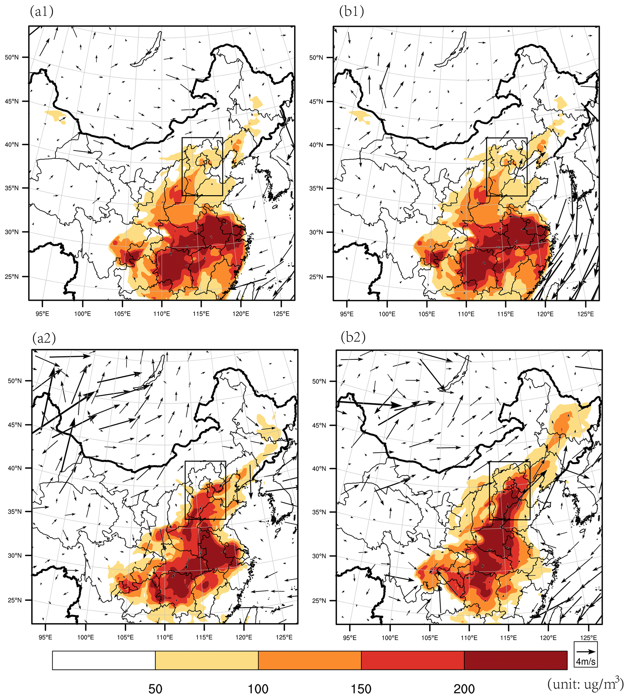
Figure 4The surface wind (vector; m s−1) and PM2.5 concentration (shaded; µg m−3) components of the initial states for the simulation of the event during 30 November and 4 December in 2018 (1) and their evolutions at the lead time 18 h (2), where the initial time is 00:00 BJT on 30 November 2018 and. Panel (a) is initialized by ERA5, and panel (b) is initialized by the GFS.
To quantify the different sensitivities of the two simulations on the initial meteorological conditions, the root mean square error (RMSE) and correlation coefficients (CCs) between the simulation and observation of the eight events are calculated. It is found that, of all eight events, the ERA5 simulations show smaller RMSEs and higher CCs with respect to the observations (see Table 1). If we take an average of the eight events for the whole simulation period (see Table 1 and Fig. 3), then the RMSE of the ERA5 and GFS simulations are 41.16 and 59.83 µg m−3, respectively; the CCs of the ERA5 and GFS simulations reach 0.79 and 0.50, respectively. Thus, for all heavy haze events considered, the simulations initialized by ERA5 reanalysis perform better than the GFS forecast data. In fact, since the ERA5 reanalysis data were obtained by assimilating all available observations with a more advanced model by the ECMWF, it has a much higher quality and is often regarded as an approximation to the real atmosphere. It is therefore comprehensible that the ERA5 performs much better in simulating the PM2.5 concentrations. This also indicates that the PM2.5 forecasting uncertainties made by the WRF-NAQPMS are highly sensitive to meteorological initial conditions, and a much accurate meteorological initial condition is essential for PM2.5 forecasts. Although the simulations initialized by ERA5 reanalysis perform better than the GFS forecast data, they still depart from the observations. Therefore, when considering the sensitivity of the meteorological field accuracy on PM2.5 concentration simulations, it is necessary to identify the sensitive area of the meteorological initial field for PM2.5 forecasts and assimilate additional targeted observations, thus pushing the PM2.5 simulation that results from the ERA5 reanalysis closer to the truth.
3.2 The sensitive areas of meteorological initial fields for PM2.5 forecasts
From Fig. 3, it is known that when the haze started to develop, it usually took more than 2 d to accumulate and dissipated rapidly in a few hours. For example, for the event that occurred during the period from 00:00 BJT (Beijing time; UTC+8 h) on 9 December to 12:00 BJT on 13 December 2016, the haze started to accumulate at approximately 20:00 BJT on 9 December, and it took 55 h to accumulate a PM2.5 concentration from 45 to 208 µg m−3. This high PM2.5 concentration was sustained for almost 16 h; then, from 18:00 BJT on 12 December, the PM2.5 concentration decreased from 217 to 46 µg m−3 in 18 h. Certainly, the stable atmospheric boundary layer will lead to the accumulation of PM2.5, while the dissipation is mostly attributed to strong winds or wet deposition (Chen et al., 2020). These distinct mechanisms may indicate that the sensitive areas of the meteorological initial field are different for the PM2.5 forecasts during the accumulation and dissipation processes. Yang et al. (2022) investigated the vertical energy profiles of the most sensitive meteorological initial perturbations (i.e., the CNOP-type error) of the PM2.5 forecasts in one heavy haze event in the BTH, and they showed that, for the forecasts during either accumulation or dissipation processes, the large energy of the CNOP-type errors mainly lies at the low level of the atmosphere for a lead time of 24 h and at the ground level for a lead time of 12 h. It is indicated that the uncertainties in the ground meteorological initial conditions may play a more important role in the PM2.5 forecasts with the lead time of 12 h. To further assess the role of the ground meteorological initial fields on the PM2.5 forecasts, we calculated the CNOP-type errors for the eight heavy haze events in this study, as Yang et al. (2022) did, and found that the PM2.5 forecast uncertainties are indeed much more sensitive to the accuracy of the initial ground meteorological conditions for the lead time 12 h (details are omitted here because of similar thoughts to those found in Yang et al., 2022). This result, relative to the economic property of the targeted observation strategy (see Sect. 1), inspires us to investigate the current ground meteorological stations within and around the BTH and to see if they can be refined to improve the PM2.5 forecasts more cost-effectively in the heavy haze events by exploring the sensitive areas of the ground meteorological field forecasting. It is expected that a station network with fewer stations will be provided, and assimilating these fewer station observations can lead to the PM2.5 forecasting skill comparable to, and even higher than, that obtained by assimilating all constructed station observations.
To do so, we consider the forecasts with the fixed lead time of 12 h but with different start times. For each event, we analyze four cycle forecasts every 12 h from its start time (see Table 2) over the accumulation process (hereafter AFs) and two forecasts over the dissipation process (hereafter DFs). As a result, a total of 32 AFs and 16 DFs was obtained for the eight events under investigation. To identify the sensitive areas of the ground meteorological field in each forecast, we adopt the idea of Lorenz (1965); this means that when the effect of initial error growth is explored, then an assumption of a perfect model is done. However, in reality, whatever the initial field of model may be, even in the case of emission inventories, it certainly consists of uncertainties. So to make our findings realistic, we have to take the better simulation initialized by ERA5 as the “truth” run because we cannot obtain relevant observations from the monitoring center for assimilations and use poorer simulation initialized by the GFS forecast data as being either the control forecast or the control run. The differences between them reflect the sensitivities of the forecast uncertainties in the PM2.5 concentrations on the accuracy of initial meteorological field. Therefore, when one computes the CNOP-type initial perturbation that is superimposed on the better simulation initialized by ERA5 (i.e., truth run), then it can be regarded as an approximation of the most sensitive initial error that disturbs the meteorological forecast of the BTH region and thus the PM2.5 forecast result. According to this perturbation, we can determine the sensitive area of the meteorological field (see the next paragraph), and preferentially assimilating additional observations in the sensitive area of the control forecast will take an updated forecast (hereafter “assimilation run”) approach to the truth run (see Yang et al., 2022). Such an idea is a kind of observation system simulation experiment (OSSE; Masutani et al., 2010). It is conceivable that if the real observations are available, then assimilating the real observations on the sensitive areas of the ERA5 simulation will also make the ERA5 simulation much closer to the real truth. In our study, we adopt this idea to determine the sensitive areas. Since the real meteorological observations are not in the public archive, additional observations are correspondingly taken from the initial field of the truth run (i.e., the ERA5 data) and called the simulated observations according to the OSSEs. These simulated observations include the wind, temperature, and relative humidity variables, and they are all the standard meteorological variables monitored in the national meteorological stations. The relevant assimilations are performed by the WRF-3DVar schemes.
Table 2Start times of the cycling AFs and DFs for the eight heavy haze events.
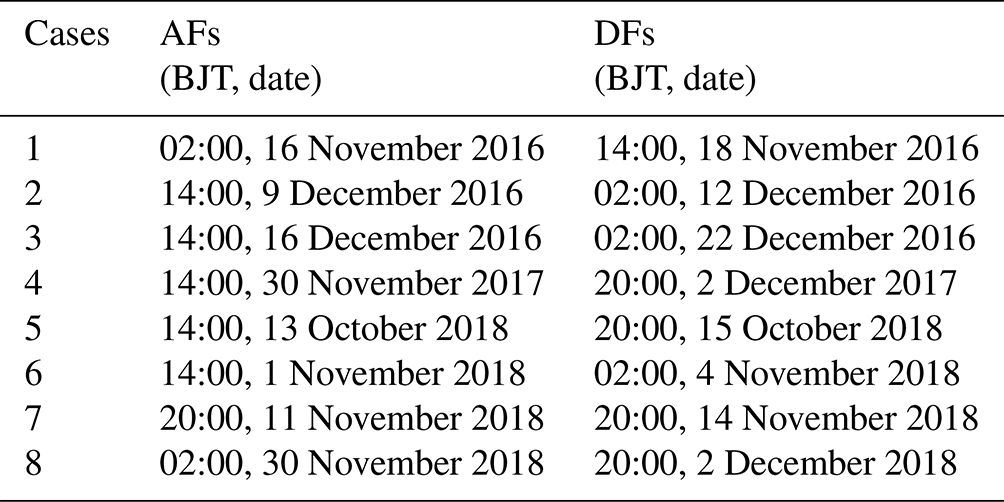
Now we determine the sensitive areas of the ground meteorological field associated with PM2.5 forecasts in the BTH. For this purpose, the CNOP-type initial errors which include the wind, temperature, and water vapor mixing ratio components at the ground level are calculated for each of the 48 PM2.5 forecasts in the truth run, with the application of WRF and its adjoint model by using the SPG2 solver (see Sect. 2). Then, a total of 48 CNOP-type initial errors are obtained for the 48 forecasts, including 32 AFs and 16 DFs. For the AFs, the CNOP-type errors are basically concentrated within the BTH region, although positioning differences exist among the forecasts. For the DFs, the CNOP-type errors are mostly located on the northern part of the BTH region, but the specific structures are dependent on the starting time. Figure 5 shows two examples of the CNOP-type errors with the wind and temperature components during AFs and DFs for the heavy haze event that occurred during 1–5 November 2018, respectively. It can be seen that, for the AFs starting from 02:00 BJT on 2 November 2018, the CNOP-type error presents large southerly wind anomalies in the southern part of the BTH region, particularly in the cities of Anyang and Liaocheng, and large negative temperature anomalies are almost located within the BTH region. For the AFs that started from 14:00 BJT on 2 November 2018, the large southerly wind errors are dominant in the city of Jining in the Shandong province, while the negative temperature error concentrates in the southern part of Hebei region. As for the two examples of the CNOP-type errors in the DFs, one is for the forecast initialized at 02:00 BJT on 4 November 2018 that exhibits large northerly wind and negative temperature anomalies in the northern part of the BTH region, covering the region of Abag Banner, with much larger temperature anomalies in the southern part of the Shandong province. The other example is for the forecast at 02:00 BJT on 5 November 2018 that presents northerly winds and negative temperature anomalies over the northern part of the Hebei province. It is obvious that the CNOP-type errors, though they are all mainly presented around the BTH region, provide different areas in which different meteorological variable errors are concentrated, even for the same forecast. To overcome this mishap, we evaluate the total moist energy norm (TME; Yang et al., 2022) of the CNOP-type errors.
The TME considers all of the concerned meteorological variables in the CNOP-type errors and measures the comprehensive sensitivity of the PM2.5 forecast uncertainties in the initial meteorological perturbations. Then the PM2.5 forecasts are more sensitive to the combined effect of all the meteorological variables' uncertainties that occurred in the area with larger values of TME, and these areas are regarded as the sensitive areas (see Yang et al., 2022). Figure 6 shows the spatial distribution of the TME for the four forecasts mentioned above. It is seen that, for the two AFs, their sensitive areas (i.e., the areas with larger values of TME) are mostly located in the BTH region, especially in Beijing city and the southern part of Hebei province. But for the forecast that started from 02:00 BJT on 2 November in them, the area in the center of Shandong province is also additionally denoted as a sensitive area. For the two DFs, their sensitive areas, compared with those of the two AFs, move northward, and the one in the forecast that initialized at 02:00 BJT on 4 November is mostly located in the provinces of Inner Mongolia and Liaoning (western part), while the other forecast presents its sensitive area closer to the BTH region, which is mostly located in the cities of Chengde and Zhangjiakou in Hebei province.
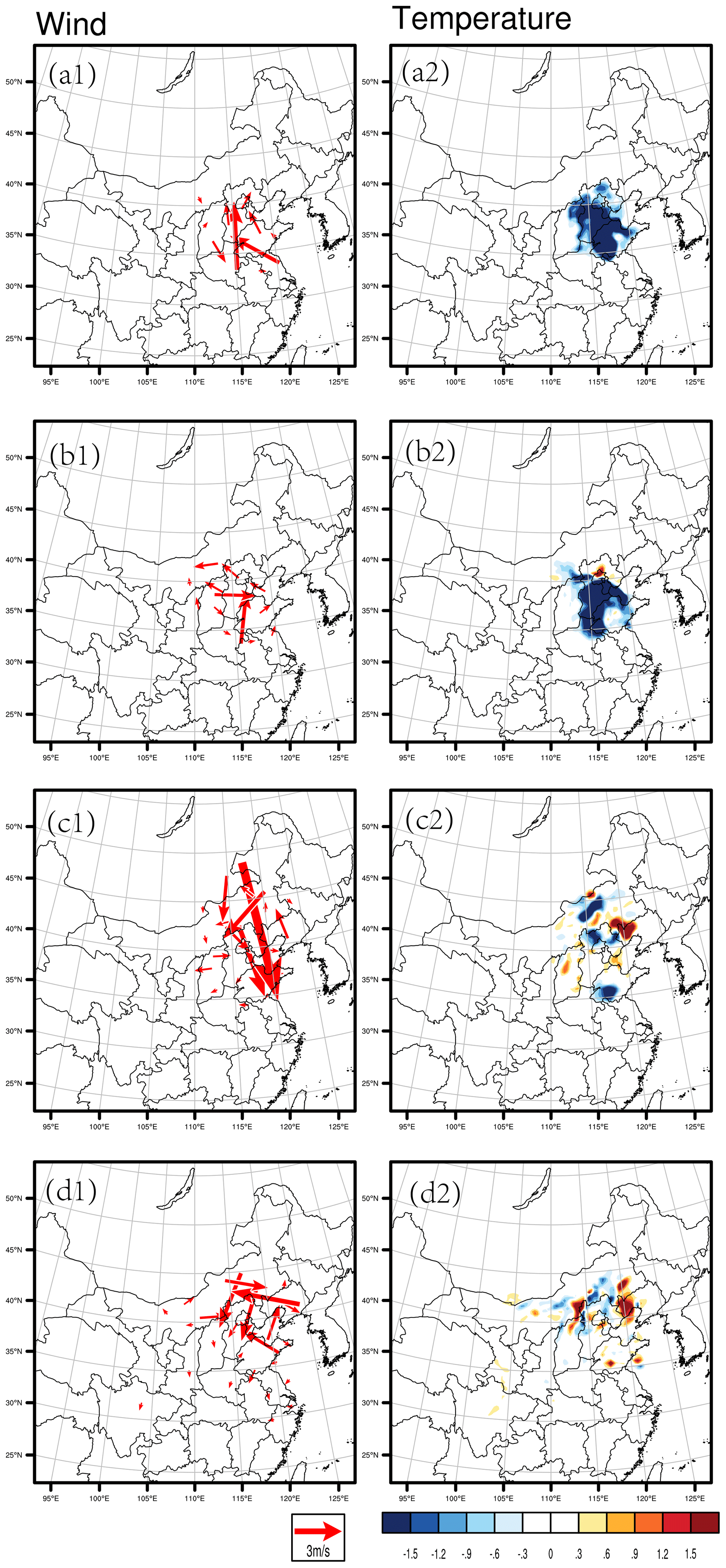
Figure 5The horizontal distribution of the wind (1) and temperature (2) components of the CNOP-type errors for the AFs that started from 02:00 BJT on 2 November (a) and from 14:00 BJT on 2 November 2018 (b) and for the DFs that started from 02:00 BJT on 4 November (c) and from 14:00 BJT on 4 November 2018 (d).
Figure 6The horizonal distribution of the TME (units in J kg−1) for the AFs starting from (a) 02:00 BJT on 2 November and (b) 14:00 BJT on 2 November 2018 and for the DFs starting from (c) 02:00 BJT on 4 November and (d) 14:00 BJT on 4 November 2018. The black rectangle is the verification area (i.e., the BTH region).
From the sensitive areas above, it is can be seen that, even for the same event, the specific distributions of the sensitive areas are dependent on the start times of the forecasts. It is therefore conceivable that the 48 forecasts for the eight events will exhibit the sensitive areas of the multifarious structures and locations. In terms of this situation, one naturally asks how a cost-effective observation network that does the PM2.5 forecasts starting from different initial times for different events can be made. Relative to the ground meteorological stations in China that are of interest for this study, the above question can be refined to ask how one can adapt the current meteorological stations within and around the BTH and make them more cost-effective in their application for the improvement of the PM2.5 forecasts with different start times for different heavy haze events. This question will be addressed in the next section.
In this section, we will construct a cost-effective meteorological observation network based on the sensitive areas identified by the CNOP-type errors in the 48 forecasts for the eight heavy haze events. Then, a series of OSSEs (see Sect. 3.2) are conducted to show the advantage of the additional observations from this observational network in improving the PM2.5 forecasting skill, which finally provides a strategy to refine the current meteorological stations within and around the BTH.
4.1 An essential observational network that enhances the PM2.5 forecasting skill greatly
For the 48 CNOP-types errors, we use a quantitative frequency method (see Duan et al., 2018) to identify the spatial grids that are often covered by large values of the TME. Specifically, for each CNOP-type error, we sort its spatial grid points in a decreasing order, according to the amplitude of the TME, and choose the first 3 % of the grid points in the model domain. Then a total of 424 grid points is obtained, which bears larger TME values than the other grid points and contributes more to the meteorological forcing errors associated with the relevant PM2.5 forecast (see Yang et al., 2022).Note that here we select the first 3 % of the grid points so that the number of sensitive grid points (424) is close to the number (481) of the current meteorological stations within and around the BTH (see Fig. 1b), in attempt to investigate whether the sensitive grid points explain the current ground stations. Since 32 AFs are considered in the study, we can obtain 32 grid point sequences from their 32 CNOP-type errors, and in each sequence, there are 424 grid points. For each grid point, we compute the frequency of each grid (i, j) occurring in the 32 sequences by Eq. (8).
where ci,j is the number of the grid point (i, j) occurring in all sequences, and N denotes the number of all sequences (here it is 32). We define a threshold of 60 % and select the grid points with F larger than 60 %, which means that the grid point (i, j) exists in most of the sequences. Then a total of 174 grid points is determined. These 174 grid points are mostly carrying many large meteorology errors measured by the TME in the 32 CNOP-type errors for the 32 AFs. Similarly, we also obtain 184 grid points from the 16 CNOP-type errors in the 16 DFs (Fig. 7a, b). We incorporated the 174 grid points for the AFs and the 184 grid pints for the DFs into an integrated observation network, as compared with the current ground meteorological stations that have been constructed within and around the BTH region (34–46∘ N, 110–120∘ E; see Fig. 1b). It is found that the meteorological stations have been constructed with 99 stations in the area covered by 174 grid points for the AFs and with 60 stations in the area covered by 184 grid points for the DFs. Since these 99 stations for AFs and 60 stations for DFs, a total of 127 stations (32 stations overlap), are all located in the area covered by the sensitive 174 grid points for AFs and 184 grid pints for DFs, they could provide additional observations that help significantly improve the skill of the PM2.5 forecast in the BTH, as compared with other constructed stations (but not in the sensitive grids). For this reason, we regard the network spanned by these 127 stations as an “essential network” (see Fig. 7c).
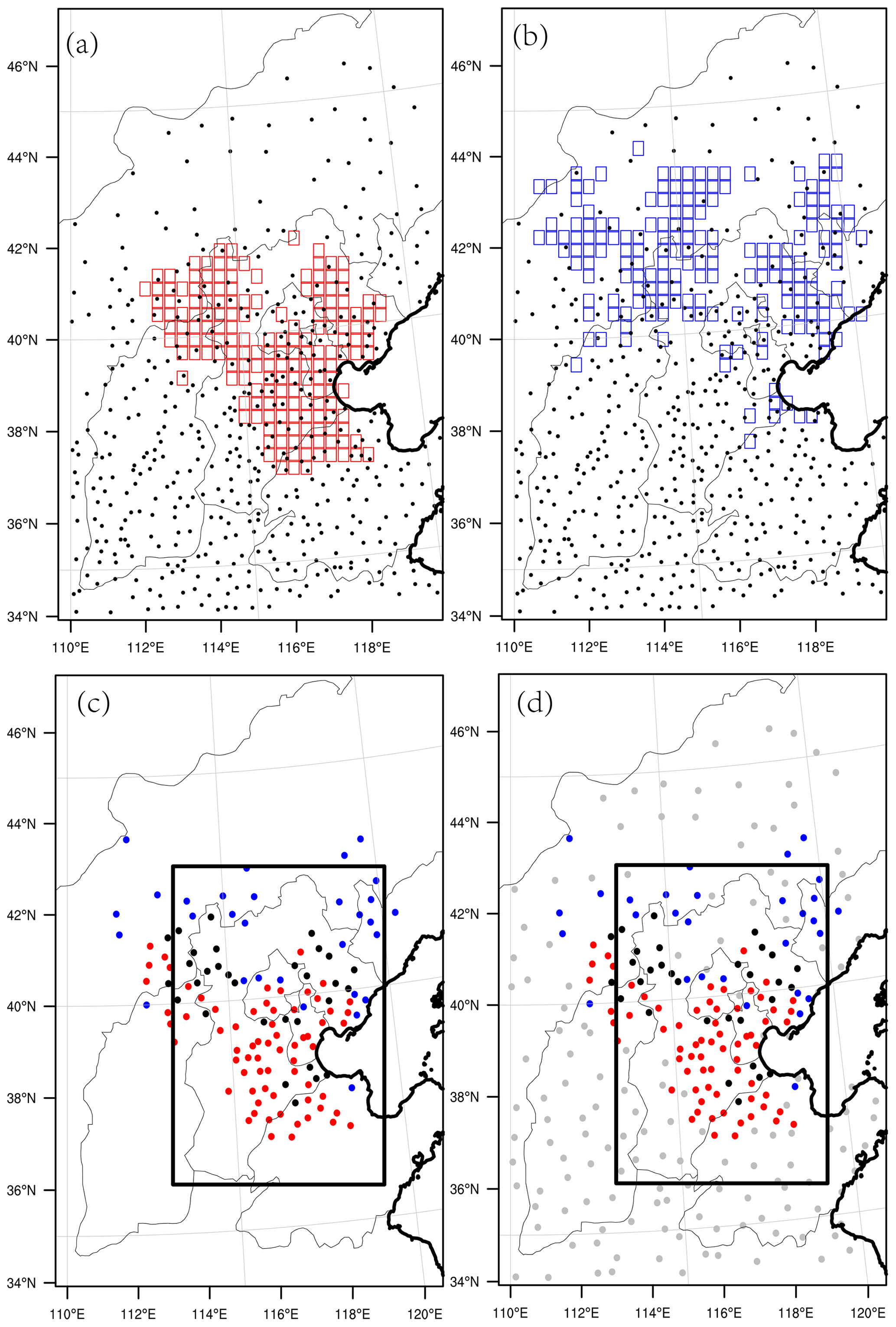
Figure 7The spatial distributions of the 174 sensitive grid points (red squares) for AFs (a), the 184 sensitive grid points (blue squares) for DFs (b), and all constructed stations (denoted by black dots in panels a and b). The contrast between the essential stations for AFs (red dots) and those for DFs (blue dots) (c) is shown, where the thick black dots present their overlapping stations. Panel (d) shows the cost-effective stations' network, including the essential stations (blue, red, and black dots) as in panel (c), and the additional scattered stations (gray dots).
Now we investigate how much this essential network can explain the skill improvement of the PM2.5 forecasts when assimilating the data acquired from all the current ground meteorology stations in and around the BTH. As mentioned in Sect. 3.2, we have to assimilate simulated observations taken from the ERA5 due to the unavailable real observations. Together with the simulated observations, we assimilate them from the essential stations and those from all the ground stations within and around the BTH to the control run generated by the GFS. Then comparisons between the assimilation runs and the control runs can be made from the perspective of AEV and AEM in Eqs. (7) and (8) in attempt to show the role of the assimilated observations in improving the PM2.5 forecasting skill.
where AEV and AEM measure the reduction rate of the errors in the control forecast at verification times (T; see Eq. 7) and that during the whole forecast period (from t0 to T; see Eq. 8) after the assimilation. The PC, PT, and PA denote the surface PM2.5 concentration in the control run, truth run, and assimilation run, respectively. The sign |⋅| means the absolute value of the forecast errors averaged over the BTH region.
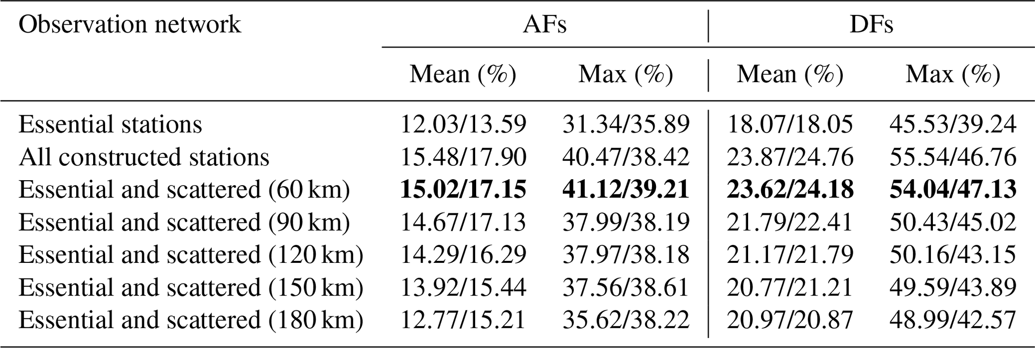
For the 32 AFs, when assimilating the 99 simulated observations, the overall improvements are 12.03 % and 13.59 %, as measured by AEV and AEM, respectively. An average of 57 % of the grids in the BTH area shows positive AEV values, and 54 % of the grids show positive AEM values; particularly, the forecast with the largest forecast error among the 32 AFs presents a reduction rate of the error by 31.34 % at the forecast time, even with approximately 76 % of the grid points in the BTH area showing a positive improvement (see Fig. 8 and Table 3). For the 16 DFs, assimilating the simulated observations at the 60 essential stations can improve the PM2.5 forecasting skill with the AEV, varying from 4.12 % to 45.53 % (exactly from 0.57 to 15.18 µg m−3), and the AEM, varying from 0.03 % to 39.24 % (exactly from 0.34 to 7.77 µg m−3). The forecast errors are reduced by an average of 18.07 % at the forecast times and 18.05 % during the whole forecast period. It is indicated that, for either AFs or DFs, their respective essential stations can provide additional observations that significantly increase the PM2.5 forecasting skill in the BTH region. Moreover, when the overall improvements are relative to those of 15.48 % and 17.90 % (measured by AEV and AEM) for AFs and of 23.87 % and 24.76 % for DFs when assimilating the simulated observations taken from all the constructed stations within and around the BTH (a total of 481 stations), they can account for at least 75 % of the latter, although the former essential stations only cover at most 20.58 % of the latter ground stations. It is clear that the essential stations can indeed provide additional observations that help increase the skill of the PM2.5 forecast in the BTH more significantly. Therefore, the essential stations are indeed crucial for the improvement of the PM2.5 forecasts in the BTH.
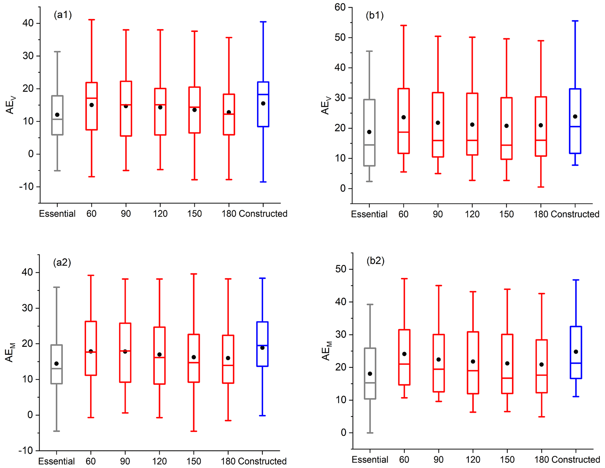
Figure 8The box plot of the (1) AEV and (2) AEM values when assimilating the essential station observations, the essential observations plus the scattered station observations with the distances 60, 90, 120, 150, and 180 km, and all constructed station observations for the (a) AFs and (b) DFs.
Table 3The mean and maxima of the improvements measured by for the AFs and DFs when the simulated observations on different observation networks are assimilated. The largest improvements among AFs or DFs for the refined observation networks are marked in bold, respectively.
4.2 The cost-effective observation network for significantly improving the PM2.5 forecast in the BTH
The essential network has been shown to play the dominant role in the improvement of the PM2.5 forecast in the BTH when compared with the assimilation of the simulated observations taken from all constructed stations, but we notice that non-negligible differences still exist between the improvements achieved by assimilating the essential observations and those that assimilate all observations. Therefore, based on the current conditions of all the constructed stations, we would refine the observations to provide a cost-effective observation network that almost fully accounts for the total improvement in the PM2.5 forecasts achieved by assimilating all the observations but brings fewer observations to the assimilation. For this purpose, we would base our observations on the essential stations to further include relatively important stations from the remaining constructed ground stations (a total of 354 stations, which are defined by the exclusion of the 127 essential stations from the constructed 481 stations). For the remaining constructed stations, they are all also located on the areas covered by the CNOP-type errors for AFs and DFs but are ruled out of the first 3 % grid points and therefore have very small errors. That is to say, the remaining stations are not essential for AFs or for DFs, and it is hard to distinguish whether they are more sensitive to AFs or DFs. For example, the southwestern part of Shandong province is covered by some of the remaining stations, but it is not only located on the area covered by the CNOP-type error in the AFs initialized at the 14:00 BJT on 2 November 2018 but also lies in the area of the CNOP-type error for the DFs starting from the 14:00 BJT on 4 November 2018 (see Fig. 6a, c). Therefore, to determine the usefulness of the remaining stations for AFs and DFs, we do not distinguish which one of them is particularly important for AFs or DFs but use the comprehensive sensitivity (rTME) defined by Eq. (9) to balance its role for both AFs and DFs.
where TMEi(AF) and TMEi(DF) represent the TME (see the Eq. 5) of the AFs and DFs, respectively. n1 and n2 are the numbers of the AFs and DFs, which are 32 and 16. Since the number of AFs is twice that of the DFs, we define the weight coefficients and w2=1. Thus, the sensitivity defined by the rTME could be proportional to the AFs and DFs, and the grid points with larger rTME are expected to provide the additional observations that, on the whole, contribute more to the reduction in the forecast errors for AFs and DFs. Despite this, the number of grid observations needed to account for better forecasting skill is also a challenging problem, especially for those observations located on the nonsensitive grid points with small CNOP-type errors. As shown by Liu and Rabier (2002), for a dense observation network with strongly correlated error in the assimilation scheme, increasing the observation density may even decrease the quality of the analysis states and further decay the forecasting skill. Particularly for the remaining ground stations mentioned above, they locate the area covered by small errors in the CNOP-type error patterns and are therefore less sensitive to PM2.5 forecast uncertainties. Then a worse forecast may come by when the impacts of the error correlations between the nearby observations overweigh the sensitivities. Therefore, a decrease in the observation density for the remaining stations is necessary to avoid impairing the analysis in the assimilation process. In fact, Yang et al. (2014) suggested that assimilating the observations with an appropriate observational distance helps one derive more benefits from the forecasts (see also Li et al., 2010; Zhang et al., 2019, and Yang et al., 2022). Therefore, when we select relatively important stations from the remaining stations by sorting the grid points according to the sensitivity provided by the rTME, we should simultaneously consider the effect of the station distances. To achieve this, we attempt to scatter the remaining stations (354 in total) across distances of 60, 90, 120, 150, 180 km and select the grid point with much larger values of rTME, as defined by Eq. (9), to determine the required stations. Note that if the distance between the scattered stations is set to be smaller than 60 km, then all of the remaining stations will be included, which is inconsistent with the aim of refining the system. We take the scatter distance of 60 km as an example to show how to select the required stations. Because the real station locations do not match the grid points in the model, we take the rTME value of their closest grid point as an approximation of their sensitivities. Therefore, for the remaining constructed ground stations, the station whose closest grid point has the largest rTME is taken as the first selected ground station; then, we exclude the stations no further than 60 km away from the first selected station and determine the station with the largest rTME among the rest of the stations as being the second selected station. After the second station is determined, we further exclude the stations no further than 60 km away from the second station and selected the third station, according to the rTME of its closest grid point; the other stations are similarly determined. Finally, a new observation network can be constructed by the combination of the essential stations and the scattered stations (see Fig. 7d).
The simulated observations (i.e., the ERA5 data) taken from the new observation networks are assimilated to the control run to show the improvements achieved by assimilating the additional observations, where it is noted that since the essential stations responsible for DFs alone are not sensitive to the AFs, these stations are also scattered with corresponding distances, according to the rTME when implementing the AFs. The same procedures are also carried out for the DFs. Specifically, on the basis of the essential stations, if the scattered stations are included with a distance of 60 km, then the performance of the PM2.5 forecasts for 32 AFs and 16 DFs is totally improved from 12.03 % to 15.02 % and from 18.07 % to 23.62 %, as measured by AEV. Meanwhile, the AEM increases from 13.59 % to 17.15 % and from 18.05 % to 24.18 %, as averaged by all the AFs and DFs, respectively (see Fig. 8 and Table 3). If a comparison is made between the essential stations and the additional scattered stations, then it is found that the latter contributes an improvement of 2.99 % and 3.56 % to the PM2.5 forecasts measured by the AEV and AEM averaged for all the AFs and an improvement of 5.55 % and 6.13 % for all DFs, which, from another perspective, emphasizes the dominant role of the essential stations in improving the PM2.5 forecasts. For the scattered stations with other distances above, we also do similar experiments and make comparisons with those scattered by the distance of 60 km, eventually showing that the stations scattered by 60 km perform the best in terms of enhancing the PM2.5 forecasting skill for either AFs or DFs. However, we also find that there are not big differences among the skill scores achieved by them. For example, when the additional stations are scattered from 60 to 90 km (correspondingly, the station number is further decreased by 83), the overall improvements of the AFs are only reduced by 0.35 %, as measured by AEV, and 0.02 %, as measured by AEM, while for the DFs, when the additional stations are scattered further than 90 km, it is even difficult to differentiate the effects between the 120 to 180 km distances. These imply that a saturation of the error reduction may exist in the given framework. In fact, Morss et al. (2001) demonstrated that the analysis errors are often small in a certain density of the observation network, so that adding more observations only resulted in small benefits, which may explain the saturation of the error reduction in the PM2.5 forecasts here.
Now we take the observation network constructed by the combination of essential stations and the scattered stations with a distance of 60 km as the newly refined observation network (see Fig. 7d) and compare it with all of the constructed ground stations by performing the assimilation runs. We find that the resultant improvements (15.02 % for AFs and 23.62 % for DFs; see above paragraph), by assimilating the newly refined station observations, can account for 97 % and 99 % of the improvements (15.48 % for AFs and 23.87 % for DFs) achieved by assimilating all of the constructed station observations for the AFs and DFs, respectively. Particularly, among the individual forecasts, 9 of the 32 AFs and 5 of the 16 DFs even show a much better forecasting skill at the forecast times in the assimilation of the newly refined observations than in that of all the constructed ground observations. It is demonstrated that assimilating the simulated observations on the refined network can result in comparative, sometimes even higher, improvements in the PM2.5 forecasting skill, as compared with assimilating all the ground station observations within and around the BTH. Furthermore, we note that the number of the newly refined stations is at least 180 less than that of the constructed stations. All of these points indicate that, under the condition of the current ground meteorological stations, the above newly refined stations may form a cost-effective observation network that almost accounts for the total improvement in the PM2.5 forecasts achieved by assimilating all the ground observations. The cost-effective observation network may provide guidance to optimize the current ground meteorological stations; at least, it suggests a much more cost-effective assimilation strategy to increase the accuracy of the meteorological forecasts for the significant improvement of the PM2.5 forecasts in the BTH.
In this section, we interpret why assimilating the cost-effective station observations results in comparative improvements and sometimes even higher improvements in PM2.5 forecasts than assimilating all the constructed station observations. It is known that the variation in the PM2.5 concentrations is dependent on both the thermodynamical and dynamic meteorological conditions. It goes without saying that the stable thermodynamical conditions, such as low planetary boundary layer height, are favorable for the accumulation of the PM2.5 concentrations (Miao et al., 2015); furthermore, a high relative humidity (RH) will also promote the processes, such as heterogeneous chemistry and gas–particle partitioning, which are all favorable for the formation of the PM2.5. For the dynamic conditions in the BTH region, increased wind speed may conversely influence the PM2.5 forecasts. For instance, a dominant northerly wind will blow away the PM2.5 in the downtown areas of the BTH region, while southerly wind will bring more PM2.5 from the southern cities to the BTH region (Zhao et al., 2009). So the accuracy of both the thermodynamical and dynamic meteorological conditions is essential for the PM2.5 forecasts in the BTH region (see the review paper of Chen et al., 2020).
For all the AFs and DFs concerned in the study, we compare their meteorological conditions before and after the assimilations of the cost-effective station observations and all the constructed station observations, respectively. We find that the assimilation, as expected, adjusts the thermodynamical and dynamic meteorological conditions at the initial state in the control run and forecasts the meteorological condition closer to the truth run, which further improve the PM2.5 forecasting skill. In particular, we found that the improvements for the AFs are basically associated with the more accurate thermodynamical conditions in the assimilation runs, while for the DFs, the improved forecasting skill is mostly attributed to the corrections of both the dynamical and thermodynamical conditions. Furthermore, the assimilations of the cost-effective station observations and all the constructed station observations correct the meteorological conditions for the PM2.5 forecasts in a similar way, which thus causes a comparative skill of the PM2.5 forecasts between them. Specifically, we select two forecasts (i.e., the AFs initialized at 14:00 BJT on 2 November 2018 and the DFs initialized at 02:00 BJT on 15 November 2018) which possess large forecast errors in the control runs as examples to present the detailed interpretations.
For the AFs, the PM2.5 concentrations in the truth run increase from 101.54 µg m−3 at 14:00 BJT on 2 November to 143.01 µg m−3 at 02:00 BJT on 3 November, averaged over the BTH and indicating an accumulation process of the PM2.5. The control run is also able to present the accumulation process but with an underestimation of 129.92 µg m−3 at the forecast time of 02:00 BJT on 3 November (Fig. 9a). The differences between them are mainly attributed to the thermodynamical condition, since there are fewer differences in the wind components (see Fig. 10a). Therefore, we are mainly concerned with the thermodynamical condition to explain the AFs. Compared with the truth run, the control run has presented a less stable condition, with an overestimation of 45.84 m in the boundary layer height and an underestimation of 16.67 % in the RH averaged over the BTH region at the forecast time; these findings are not beneficial for the accumulation and formation of PM2.5, so an underestimation of the PM2.5 concentration comes about. When the simulated observations from all the constructed meteorological stations are assimilated, the boundary layer height has decreased and the RH has increased over the central and southern part of the BTH region at the initial time. The improved thermodynamic condition further modifies the meteorological condition at the forecast time, including a decrease of 21.56 m for the boundary layer height and an increase of 8.02 % for the RH averaged over the BTH region, both of which contribute to an increase in the PM2.5 concentrations from 129.92 to 138.85 µg m−3 averaged over the BTH region and thus an improvement in the PM2.5 forecasting skill (see Fig. 11). By comparison, the assimilation of the cost-effective station observations will modify the meteorological conditions in the same way, with a decrease of 20.95 m in boundary layer and an increase of 7.57 % in RH that finally results in an average PM2.5 of 138.60 µg m−3 at the forecast time, with only 0.25 µg m−3 lower than the forecast with the assimilation of all constructed station observations. Hence, the cost-effective network can approximate all constructed stations and provide additional observations of an equivalent efficiency for all observations in order to improve the PM2.5 forecasts in the BTH. Moreover, we also implement the PM2.5 forecasts with longer lead times for the eight heavy haze events by using the meteorological analysis field updated by assimilating the cost-effective observations. And we demonstrate that, although the cost-effective network is developed according to the sensitivity of the meteorological forecasts with the lead time of 12 h, its resultant meteorological analysis fields still have positive effects on improving the AFs with longer lead times. For example, in the AFs quoted in this section, assimilating the cost-effective station observations can reduce the forecast errors by 32.05 % and 7.81 % at the forecast time, with a lead time of 18 and 24 h, respectively; furthermore, these improvements are also approaching those achieved by the assimilation of all constructed station observations (see Figs. 9a and 11).
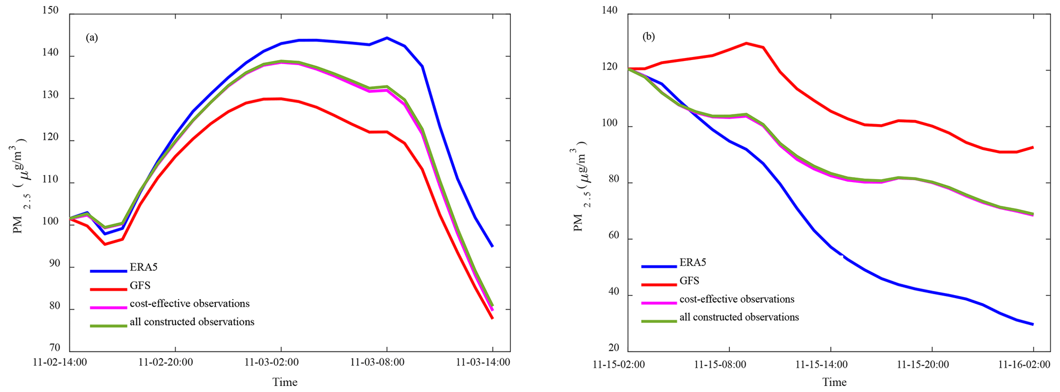
Figure 9Time series of the PM2.5 concentrations averaged over the BTH region of the truth run, the control run, and the assimilation run inherited from the cost-effective observations and all the constructed observations for the AFs initialized at 14:00 BJT on 2 November 2018, with a lead time of 24 h (a), and the DFs starting from 02:00 BJT on 15 November 2018, with a lead time of 24 h (b).
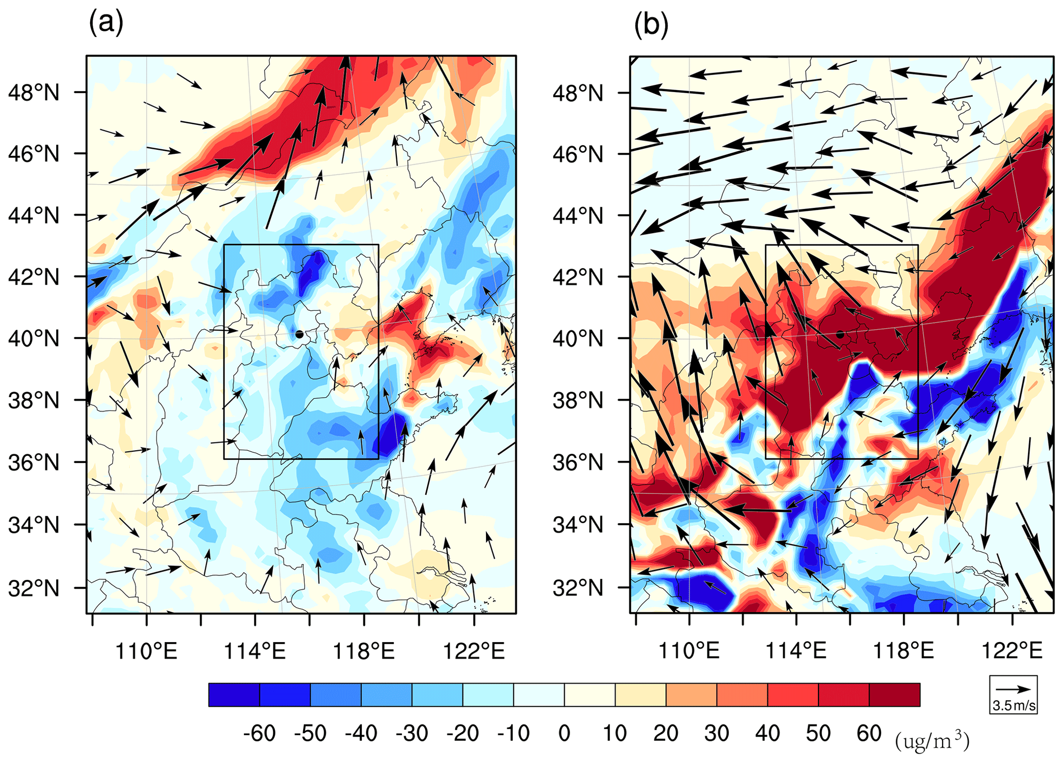
Figure 10The differences in the wind (vector; m s−1) and PM2.5 concentration (shaded; µg m−3) between the truth run and control run (control run minus truth run) for (a) the AFs at the forecast time of 02:00 BJT on 3 November 2018 and (b) the DFs at the forecast time of 14:00 BJT on 15 November 2018.
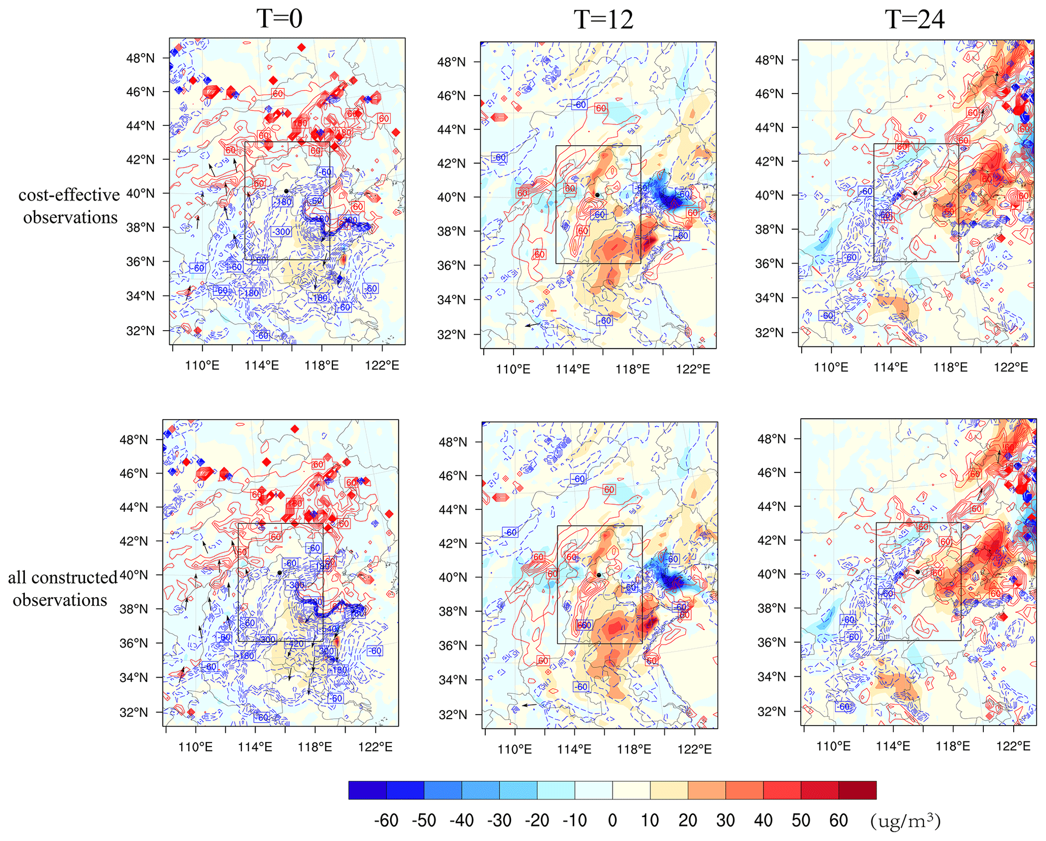
Figure 11The differences in the boundary layer height (contour line; m; blue line means reduction and red line means increase) and the PM2.5 concentrations (shaded; µg m−3) between the assimilation run inherited from the cost-effective observations and constructed observations and the control run for the AFs that started from 14:00 BJT on 2 November 2018 and with lead times of 12 and 24 h.
For the DFs, the mechanism is different from the AFs, where both thermodynamical and dynamical conditions have critical impacts on the PM2.5 variation. The PM2.5 concentrations in the truth run decreased from 120.50 µg m−3 on 15 November at 02:00 BJT to 57.19 µg m−3 on 15 November at 14:00 BJT in the BTH region. The dissipation is caused by the northerly wind in the northwestern part of the BTH region at the initial time, and then the northerly wind increased gradually with the speed of 4.92 m s−1 at the forecast time over the BTH region, which blew away the PM2.5 concentrations in the BTH. Conversely, the control run presents a southerly wind in the northern part of the BTH region and an easterly wind in the Inner Mongolia Province, which go against the truth run (Fig. 10b) and result in an overestimation of the PM2.5 with a concentration of 105.50 µg m−3 at the forecast time (Fig. 9b). Besides the dynamical reasons, the control run also presents higher relative humidity biases over the BTH region, which also contributes to the overestimation of PM2.5 concentrations. When the simulated observations from all the constructed stations are assimilated to the initial state, the northwesterly wind increases in the northern part of the BTH region at the initial time, and at the forecast time the northerly wind over the BTH region has increased to 2.73 m s−1. Meanwhile, the assimilation also results in a decrease in the RH from 76.28 % to 73.67 %. It is obvious that the increased northerly wind and decreased RH are beneficial for the dissipation of the PM2.5, and these led to the PM2.5 concentration's decrease from 105.50 to 83.35 µg m−3 in the BTH region at the forecast time, resulting in an improvement of 45.85 % in the PM2.5 forecasting skill. When the simulated observations from the cost-effective station observations are assimilated, the meteorological conditions are modified in the same way, except for the stronger northerly wind of 2.77 m s−1 over the BTH at the forecast time. The stronger northerly wind blows more pollution in the BTH region to the downwind region so that the mean PM2.5 concentrations over the BTH region decreases to 82.53 µg m−3 and shows an improvement of 47.55 % in the PM2.5 forecasting skill at the forecast time, which is 1.7 % higher than the improvement found when all the constructed station observations are assimilated. Therefore, though fewer observations in the cost-effective network are assimilated, they result in a higher forecasting skill by reducing larger forecast errors in the northerly wind. Furthermore, similar to the AFs, with the meteorological analysis fields obtained by the cost-effect observation network, the comparative improvements of the DFs can be achieved at much longer times. Specifically in this forecast, the improvements can reach 34.16 % and 29.36 % at the lead times of 18 and 24 h, as measured by AEV, respectively, which is almost the same as the improvements in the assimilation of all constructed station observations (see Figs. 9b and 12).
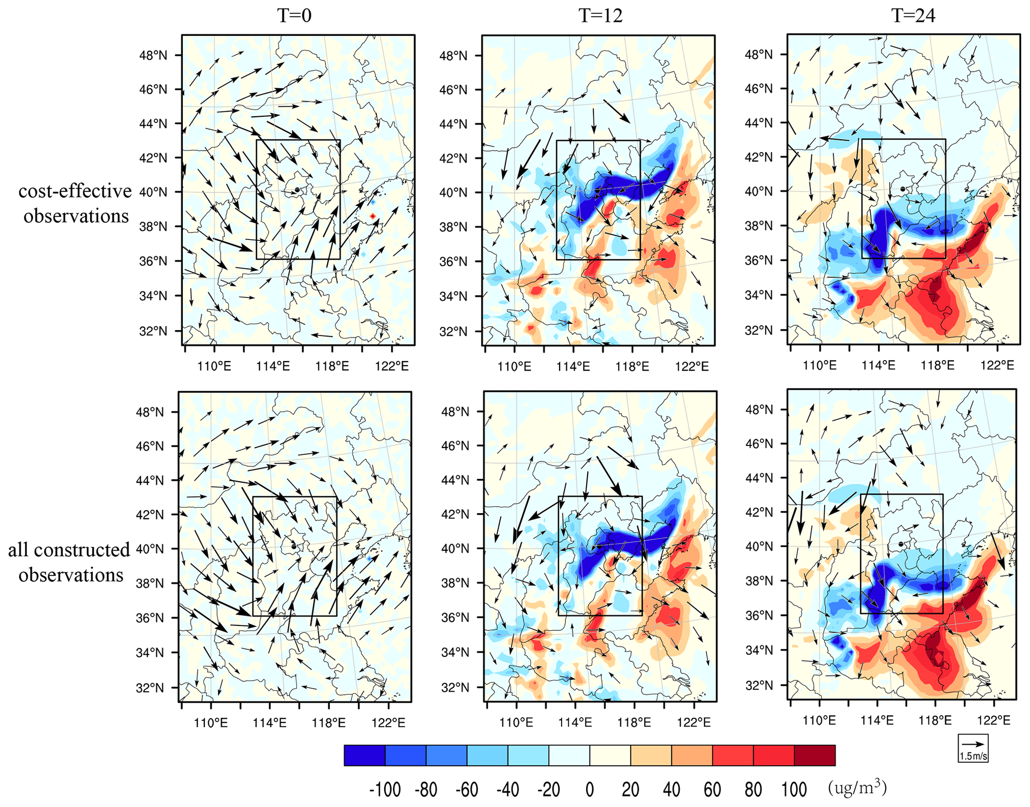
Figure 12The differences in the ground wind (vector; m s−1) and PM2.5 concentrations (shaded; µg m−3) between the assimilation run (inherited from the cost-effective observations and all constructed station observations) and the control run for the DFs that started from 02:00 BJT on 15 November 2018 and with lead times of 12 and 24 h.
So far, we have verified numerically the validity of the cost-effective ground meteorological stations' network in improving the PM2.5 forecasts of the BTH more economically by assimilating fewer observations. Also, we have interpreted this validity in terms of the perspective of dynamics and thermodynamics. It is therefore expected that the cost-effective network can provide a guidance to refine the current ground stations from the viewpoint of the PM2.5 concentration forecasts in the BTH.
The PM2.5 forecasts of the BTH region are sensitive to the meteorological initial condition, and in this study, we investigate the role of the ground meteorological stations within and around the BTH, finally proposing a strategy to refine them, which is inspired by the fact that a high density of observations is not necessary for higher forecast benefits. Specifically, a total of 32 AFs and 16 DFs obtained from all eight heavy haze events in the BTH region in the winter season during the years of 2016–2018 was investigated using the WRF-NAQPMS model, and their fastest growth initial errors (i.e., the CNOP-type errors) are calculated to identify their respective sensitive areas in the ground meteorological fields; based on these sensitive areas, a frequency method suggested by Duan et al. (2018) is used to recognize the sensitive grid points applicable for the forecasts of the PM2.5 concentrations with different start times, which provides help to refine the current ground meteorological stations (a total of 481 stations) within and around the BTH and form the newly refined stations' network (a total of 287 stations, which is 194 less than that of the former) for the PM2.5 forecasts in the BTH.
Numerically, a series of OSSEs is conducted to verify the effectiveness of the newly refined 287 station observations in terms of improving the PM2.5 forecasts in the BTH. They demonstrate that, when the additional simulated observations (i.e., the ERA5 data) from these refined stations are assimilated to the control run initialized by the GFS data, the overall PM2.5 forecasting skill increases to 15.02 % and 23.62 % at the forecast time of AFs and DFs, which have accounted for 97 % and 99 % of the improvements when the simulated observations from all the 481 ground stations are assimilated. For some individual forecasts, assimilating the simulated observations even results in better forecasting skill for PM2.5. Physically, we interpret why assimilating fewer observations from the refined stations can have an improvement in the PM2.5 forecasting skill that is comparative to, or even higher than, that of an assimilation of all of the ground station observations. In fact, assimilating fewer observations has equivalent capabilities in terms of correcting the atmospheric stability for the AFs and modifying the dynamical and thermodynamical conditions for the DFs when compared with assimilating all of the ground observations, which makes the control run closer to the truth and results in a comparative improvement in the PM2.5 forecasting skill.
It is clear that assimilating fewer sensitive observations can lead to better PM2.5 forecasting skill, which indicates that it is not necessarily the use of more densely scattered meteorological observation stations but rather that a few sensitive stations can greatly improve the PM2.5 forecasting skill. It implies that 58 % (the 279 refined stations for the AFs) of the current station observations accounting for the 97 % of the improvements at the forecast time for AFs and 50 % (the 241 refined stations for the DFs) of the current station observations contribute to the 99 % of the improvements at the forecast time for DFs. In combining the AFs and DFs, there are a total of 287 stations (about 60 % of the current stations) that remain to make highly efficient contribution to the PM2.5 forecasts in the BTH region. It is therefore indicated that the newly refined network may play a role in the cost-effective ground meteorological stations in terms of greatly improving the PM2.5 forecast in the BTH. Although the present study is associated with hindcasts of PM2.5, it is still difficult to obtain the meteorological observations from the monitoring center; therefore, we can only assimilate the simulated observations (i.e., the ERA5 data) to the control run to show the effectiveness of the cost-effective observation network. The effectiveness is verified by examining whether a forecast (i.e., the simulation initialized by GFS) after assimilating the observations from the cost-effective station network will be much closer to the good simulation (i.e., the simulation initialized by ERA5). If the cost-effective station network is useful along this thinking, it can be inferred that assimilating the real observations from the cost-effective stations to the meteorological initial field in the control forecast would improve the meteorological field forecasting and then the PM2.5 forecasting greatly against the observations. This may suggest that 287 refined stations in the study should maintain their operations and that other stations around the BTH can be greatly scattered to avoid unnecessary work. Relative to the objective of scientifically arranging the observation network proposed by the China Meteorological Administration during the 14th Five-Year Plan period, our study could provide scientific guidance for optimizing the ground meteorological station network with the respect to improving the air quality forecasts.
In this study, we focus on the effect of surface meteorological uncertainties in the PM2.5 forecast in the BTH and suggest that the current constructed ground stations can be refined to a cost-effective station network. In fact, these cost-effective stations, as demonstrated in Sect. 4, are made up of the constructed stations that appear in the area covered by the 174/184 sensitive grid points for AFs/DFs revealed by the CNOP-type errors and the scatted stations which have also been constructed but do not appear in the area covered by the sensitive grids. It is therefore conceivable that the cost-effective network in this study could be further optimized by moving the stations not located in the area covered by the sensitive grids to the area with higher sensitivities (i.e., the area covered by the 174/184 sensitive grid points). In the present study, we studied the meteorological initial uncertainties in the wind, temperature, and water vapor variables, which are conventional meteorological variables monitored at the national meteorological stations. Apart from these, the boundary layer height is a key meteorological variable for PM2.5 forecasts. Since the boundary layer simulation is more influenced by the parameterization in the WRF model (Chen et al., 2017; Mohan and Gupta, 2018) for studying the role of the boundary layer uncertainties in yielding the PM2.5 forecast uncertainties, an extension of the CNOP method, CNOP-parametric perturbation (CNOP-P; Mu et al., 2010) or the nonlinear forcing singular vector (NFSV; Duan and Zhou, 2013), can be used. It is expected that future studies could address the boundary layer uncertainties using the extensions of CNOP method, and these uncertainties may provide guidance to optimize its relevant observation network. Besides the meteorological observations, pollutant observations are also quite important for the air quality forecasts (Luo et al., 2022). Therefore, optimizing the environmental monitoring stations and obtaining more useful pollutant observations are also very important for the significant improvements in air quality forecasting, which may further reduce the gap between the forecasts and observations in the air quality studies. Though previous studies have attempted to identify the sensitive areas for the targeted observations of chemical constituents using singular vector or adjoint sensitivity methods (Daescu and Carmichael, 2003; Goris and Elbern, 2015), they used a linear approach and did not sufficiently consider the nonlinear effect of initial value sensitivity, so that implementing the observations on these sensitive areas may not lead to the largest improvements (Wang et al., 2011). The application of CNOP for determining the sensitive areas may overcome these limitations. It is therefore expected that the optimization of environmental monitoring stations can be studied in depth, and more useful conclusions will be achieved to greatly improve the forecasts of air quality in the future.
Version 3.6.1 of the WRF and its adjoint model are used in this study, and both are available from https://doi.org/10.5065/D68S4MVH (Skamarock et al., 2008). The exact version of the model to produce the results used in this paper is available on Zenodo (https://doi.org/10.5281/zenodo.7627369, Yang and Duan, 2023a). The analyzed data used in this paper are available on Zenodo (https://doi.org/10.5281/zenodo.7627556, Yang and Duan, 2023b). Hourly surface PM2.5 data are obtained from http://www.cnemc.cn/en/ (China National Environmental Monitoring Center (CNEMC), 2022). The ERA5 reanalysis product is available at https://www.ecmwf.int/en/forecasts/datasets/reanalysis-datasets/era5 (Hersbach et al., 2017; login required). The NCEP GFS product is available at https://doi.org/10.5065/D65D8PWK (NCEP, 2015).
YL and DW conceived the research, designed the experiments, performed the simulations, and analyzed the results. All authors contributed to drafting the paper.
The contact author has declared that none of the authors has any competing interests.
Publisher's note: Copernicus Publications remains neutral with regard to jurisdictional claims in published maps and institutional affiliations.
The authors highly appreciate the two anonymous reviewers and Jie Feng, who provided constructive comments that greatly improved the overall quality of the paper.
This research has been supported by the National Natural Science Foundation of China (grant nos. 42105061).
This paper was edited by Havala Pye and reviewed by two anonymous referees.
Bei, N., Wu, J., Elser, M., Feng, T., Cao, J., El-Haddad, I., Li, X., Huang, R., Li, Z., Long, X., Xing, L., Zhao, S., Tie, X., Prévôt, A. S. H., and Li, G.: Impacts of meteorological uncertainties on the haze formation in Beijing–Tianjin–Hebei (BTH) during wintertime: a case study, Atmos. Chem. Phys., 17, 14579–14591, https://doi.org/10.5194/acp-17-14579-2017, 2017.
Bengtsson, L. and Gustavsson, N.: Assimilation of nonsynoptic observations, Tellus, 24, 383–399, 1972.
Birgin, E. G., Martinez, J. M., and Raydan, M.: Algorithm 813: SPG – software for convex-constrained optimization, ACM. Trans. Math. Softw., 27, 340–349, 2001.
Bishop, C., Etherton, B. J., and Majumdar, S. J.: Adaptive sampling with the ensemble transform Kalman filter. Part I: Theoretical aspects, Mon. Weather Rev., 129, 420–436, 2001.
Chen, B., Mu, M., and Qin, X. H.: The Impact of Assimilating Dropwindsonde Data Deployed at Different Sites on Typhoon Track Forecasts, Mon. Weather Rev., 141, 2669–2682, 2013.
Chen, D., Xie, X., Zhou, Y., Lang, J., Xu, T., Yang, N., Zhao, Y., and Liu, X.: Performance evaluation of the WRF-CHEM model with different physical parameterization schemes during an extremely high PM2.5 pollution episode in Beijing, Aerosol Air Qual. Res., 17, 262–277, 2017.
Chen, Z., Chen, D., Zhao, C., Kwan, M., Cai, J., Zhuang, Y., Zhao, B., Wang, X., Chen, B., Yang, J., Li, R., He, B., Gao, B., Wang, K., and Xu, B.: Influence of meteorological conditions on PM2.5 concentrations across China: A review of methodology and mechanism, Environ. Int., 139, 105558, https://doi.org/10.1016/j.envint.2020.105558, 2020.
China National Environmental Monitoring Centre (CNEMC): Air quality data in China, CNEMC [data set], http://www.cnemc.cn/en/ (last access: 10 January 2023), 2022.
Daescu, D. N. and Carmichael, G. R.: An Adjoint Sensitivity Method for the Adaptive Location of the Observations in Air Quality Modeling, J. Atmos. Sci., 60, 434–450, https://doi.org/10.1175/1520-0469(2003)060<0434:AASMFT>2.0.CO;2, 2003.
Devers, A., Vidal, J.-P., Lauvernet, C., Graff, B., and Vannier, O.: A framework for high-resolution meteorological surface reanalysis through offline data assimilation in an ensemble of downscaled reconstructions, Q. J. Roy. Meteor. Soc, 146, 153–173, https://doi.org/10.1002/qj.3663, 2020.
Duan, W. and Zhou, F.: Non-linear forcing singular vector of a two-dimensional quasi-geostrophic model, Tellus, 65, 256–256, 2013.
Duan, W., Li, X., and Tian, B.: Towards optimal observational array for dealing with challenges of El Niño-Southern Oscillation predictions due to diversities of El Niño, Clim. Dynam., 51, 3351–3368, https://doi.org/10.1007/s00382-018-4082-x, 2018.
Duan, W., Yang, L., Mu, M., Wang, B., Shen, X., Meng, Z., and Ding, R.: Recent advances in China on the predictability of weather and climate, Adv. Atmos. Sci., 40, 1521–1547, https://doi.org/10.1007/s00376-023-2334-0, 2023.
Dudhia, J.: Numerical study of convection observation during the winter monsoon experiment using a mesoscale two-dimensional model, J. Atmos., Sci., 46, 3077–3107, https://doi.org/10.1175/1520-0469(1989)046<3077:NSOCOD>2.0.CO;2, 1989.
Ehrendorfer, M., Errico, R. M., and Raeder, K. D.: Singular-Vector Perturbation Growth in a Primitive Equation Model with Moist Physics, J. Atmos. Sci., 56, 1627–1648, https://doi.org/10.1175/1520-0469(1999)056<1627:SVPGIA>2.0.CO;2, 1999.
Feng, J., Qin, X., Wu, C., Zhang, P., Yang, L., Shen, X., Han, W., and Liu, Y.: Improving typhoon predictions by assimilating the retrieval of atmospheric temperature profiles from the FengYun-4A's Geostationary Interferometric Infrared Sounder (GIIRS), Atmos. Res., 280, 106391, https://doi.org/10.1016/j.atmosres.2022.106391, 2022.
GBD 2017 Risk Factor Collaborators: Global, regional, and national comparative risk assessment of 84 behavioural, environmental and occupational, and metabolic risks or clusters of risks for 195 countries and territories, 1990–2017: a systematic analysis for the Global Burden of Disease Study 2017, Lancet, 392, 1923–1994, 2018.
Gilliam, R. C., Hogrefe, C., Godowitch, J. M., Napelenok, S., Mathur, R., and Rao, S. T.: Impact of inherent meteorology uncertainty on air quality model predictions, J. Geophys. Res.-Atmos., 120, 12259–12280, 2015.
Goris, N. and Elbern, H.: Singular vector-based targeted observations of chemical constituents: description and first application of the EURAD-IM-SVA v1.0, Geosci. Model Dev., 8, 3929–3945, https://doi.org/10.5194/gmd-8-3929-2015, 2015.
Hersbach, H., Bell, B., Berrisford, P., Hirahara, S., Horányi, A., Muñoz‐Sabater, J., Nicolas, J., Peubey, C., Radu, R., Schepers, D., Simmons, A., Soci, C., Abdalla, S., Abellan, X., Balsamo, G., Bechtold, P., Biavati, G., Bidlot, J., Bonavita, M., De Chiara, G., Dahlgren, P., Dee, D., Diamantakis, M., Dragani, R., Flemming, J., Forbes, R., Fuentes, M., Geer, A., Haimberger, L., Healy, S., Hogan, R.J., Hólm, E., Janisková, M., Keeley, S., Laloyaux, P., Lopez, P., Lupu, C., Radnoti, G., de Rosnay, P., Rozum, I., Vamborg, F., Villaume, S., and Thépaut, J.-N.: Complete ERA5 from 1979: Fifth generation of ECMWF atmospheric reanalyses of the global climate, Copernicus Climate Change Service (C3S) Data Store (CDS), ECMWF [data set], https://www.ecmwf.int/en/forecasts/dataset/ecmwf-reanalysis-v5 (last access: 29 June 2023), 2017.
Hong, S. Y., Ying, N., and Dudhia, J.: A new vertical diffusion package with an explicit treatment of entrainment processes, Mon. Weather Rev., 134, 2318–2341, https://doi.org/10.1175/MWR3199.1, 2006.
Hu, Y. W., Zang, Z. L., Ma, X. Y., Liang, Y. F., Zhao, D. C., and You, W.: Research on the effects of assimilation meteorological observation data on aerosol concentration, China Environmental Science, 39, 523–532, 2019 (in Chinese).
Huang, X., Ding, A. J., Gao, J., Zheng, B., Zhou, D. R., Qi, X. M., Tang, R., Wang, J. P., Ren, C. H., Nie, W., Chi, X. G., Xu, Z., Chen, L. D., Li, Y. Y., Che, F., Pang, N. N., Wang, H. K., Tong, D., Qin, W., Cheng, W., Liu, W. J., Fu, Q. Y., Liu, B. X., Chai, F. H., Davis, S., Zhang, Q., and He, K. B.: Enhanced secondary pollution offset reduction of primary emissions during COVID-19 lockdown in China, Natl. Sci. Rev., 8, nwaa137, https://doi.org/10.1093/nsr/nwaa137, 2021.
Iacono, M. J., Delamere, J. S., Mlawer, E. J., Shephard, M. W., Clough, S. A., and Collins, W. D.: Radiative forcing by long-lived greenhouse gases: calculations with the AER radiative transfer models, J. Geophys. Res.-Atmos., 113, D13103, https://doi.org/10.1029/2008JD009944, 2008.
Janjić, T., Bormann, N., Bocquet, M., Carton, J. A., Cohn, S. E., Dance, S. L., Losa, S. N., Nichols, N. K., Potthast, R., Waller, J. A., and Weston, P.: On the representation error in data assimilation, Q. J. Roy. Meteor. Soc., 144, 1257–1278, 2018.
Langland, R. H., Gelaro, R., Rohaly, G. D., and Shapiro, M. A.: Targeted observations in FASTEX: Adjoint-based targeting procedures and data impact experiments in IOP17 and IOP18, Q. J. Roy. Meteor. Soc., 125, 3241–3270, 1999.
Li, X., Zhu, J., Xiao, Y., and Wang, R. A Model-Based Observation-Thinning Scheme for the Assimilation of High-Resolution SST in the Shelf and Coastal Seas around China, J. Atmos. Ocean. Tech., 27, 1044–1058, 2010.
Lin, Y. L., Farley, R. D., and Orville, H. D.: Bulk Parameterization of the Snow Field in a Cloud Model, J. Appl. Meteorol. Clim., 22, 1065–1092, https://doi.org/10.1175/1520-0450(1983)022<1065:BPOTSF>2.0.CO;2, 1983.
Liu, C., Zhang, S., Gao, Y., Wang, Y., Sheng, L., Gao, H., and Fung, J. C. H.: Optimal estimation of initial concentrations and emission sources with 4D-Var for air pollution prediction in a 2D transport model, Sci. Total Environ., 773, 145580, https://doi.org/10.1016/j.scitotenv.2021.145580, 2021.
Liu, T., Gong, S., He, J., Yu, M., Wang, Q., Li, H., Liu, W., Zhang, J., Li, L., Wang, X., Li, S., Lu, Y., Du, H., Wang, Y., Zhou, C., Liu, H., and Zhao, Q.: Attributions of meteorological and emission factors to the 2015 winter severe haze pollution episodes in China's Jing-Jin-Ji area, Atmos. Chem. Phys., 17, 2971–2980, https://doi.org/10.5194/acp-17-2971-2017, 2017.
Liu, Z.-Q. and Rabier, F.: The interaction between model resolution, observation resolution and observation density in data assimilation: A one-dimensional study, Q. J. Roy. Meteor. Soc., 128, 1367–1386, https://doi.org/10.1256/003590002320373337, 2002.
Lorenz, E. N.: A study of the predictability of a 28 variable atmospheric model, Tellus, 17, 321–333, https://doi.org/10.3402/tellusa.v17i3.9076, 1965.
Lou, M., Guo, J., Wang, L., Xu, H., Chen, D., Miao, Y., Lv, Y., Li, Y., Guo, X., Ma, S., and Li, J.: On the relationship between aerosol and boundary layer height in summer in China under different thermodynamic conditions, Earth and Space Science, 6, 887–901, 2019.
Luo, H., Tang, X., Wu, G., Kong, L., and Coauthors. The Impact of the Numbers of Monitoring Stations on the National and Regional Air Quality Assessment in China During 2013–18, Adv. Atmos. Sci., 39, 1709–1720, 2022.
Majumdar, S. J., Bishop, C. H., Etherton, B. J., and Toth, Z.: Adaptive sampling with the ensemble transform Kalman filter. Part II: Field program implementation, Mon. Weather Rev., 130, 1356–1369, https://doi.org/10.1175/1520-0493(2002)130<1356:ASWTET>2.0.CO;2, 2002.
Masutani, M., Schlatter, T., Errico, R., Stoffelen, A., Andersson, E., Lahoz, W., Woollen, J., Emmitt, G., Riishojgaard, L., and Lord, S.: Observing System Simulation Experiments, in: Data Assimilation, edited by: Lahoz, W., Khattatov, B., and Menard, R., Springer, Berlin, Heidelberg, https://doi.org/10.1007/978-3-540-74703-1_24, 2010.
Miao, Y. C., Hu, X. M., Liu, S. H., Qian, T. T., Xue, M., Zheng, Y. J., and Wang, S.: Seasonal variation of local atmospheric circulations and boundary layer structure in the Beijing-Tianjin-Hebei region and implications for air quality, J. Adv. Model. Earth Sy., 7, 1602–1626, 2015.
Mohan, M. and Gupta, M.: Sensitivity of PBL parameterizations on PM10 and ozone simulation using chemical transport model WRF-Chem over a sub-tropical urban airshed in India, Atmos. Environ., 185, 53–63, 2018.
Morss, R. E., Emanuel, K. A., and Snyder, C.: Idealized adaptive observation strategies for improving numerical weather prediction, J. Atmos. Sci., 58, 210–232, https://doi.org/10.1175/1520-0469(2001)058<0210:IAOSFI>2.0.CO;2, 2001.
Mu, M. and Wang, J.: Nonlinear fastest growing perturbation and the first kind of predictability, Sci. China Ser. D, 44, 1128–1139, https://doi.org/10.1007/BF02906869, 2001.
Mu, M., Duan, W. S., and Wang, B.: Conditional nonlinear optimal perturbation and its applications, Nonlin. Processes Geophys., 10, 493–501, https://doi.org/10.5194/npg-10-493-2003, 2003.
Mu, M., Duan, W., Wang, Q., and Zhang, R.: An extension of conditional nonlinear optimal perturbation approach and its applications, Nonlin. Processes Geophys., 17, 211–220, https://doi.org/10.5194/npg-17-211-2010, 2010.
NCEP: NCEP GFS 0.25 Degree Global Forecast Grids Historical Archive, NCEP [data set], https://doi.org/10.5065/D65D8PWK, 2015.
Snyder, C.: Summary of an informal workshop on adaptive observations and FASTEX, B. Am. Meteorol. Soc., 77, 953–961, https://doi.org/10.1175/1520-0477-77.5.953, 1996.
Palmer, T. N., Gelaro, R., Barkmeijer, J., and Buizza, R.: Singular vectors, metrics, and adaptive observations, J. Atmos. Sci., 55, 633–653, https://doi.org/10.1175/1520-0469(1998)055<0633:SVMAAO>2.0.CO;2, 1998.
Qin, X. and Mu, M.: A Study on the Reduction of Forecast Error Variance by Three Adaptive Observation Approaches for Tropical Cyclone Prediction, Mon. Weather Rev., 139, 2218–2232, 2011.
Qin, X., Duan, W., and Mu, M.: Conditions under which CNOP sensitivity is valid for tropical cyclone adaptive observations, Q. J. Roy. Meteor. Soc., 139, 1544–1554, https://doi.org/10.1002/qj.2109, 2013.
Skamarock, W. C., Klemp, J. B., Dudhia, J., Gill, D. O., Barker, D. M., Duda, M. G., Huang, X. Y., Wang, W., and Powers, J. G.: A Description of the Advanced Research WRF Version 3, NCAR Tech. Note No. NCAR/TN-475+STR, 113 pp., https://doi.org/10.5065/D68S4MVH, 2008.
Talagrand, O.: Assimilation of Observations, an Introduction, J. Meteorol. Soc. Jpn, Ser. II, 75, 191–209, 1997.
Toth, Z. and Kalnay, E.: Ensemble Forecasting at NMC: The Generation of 1339 Perturbations, B. Am. Meteorol. Soc., 74, 2317–2330, 1993.
Wang, H., Mu, M., and Huang, X.-Y.: Application of conditional non-linear optimal perturbations to tropical cyclone adaptive observation using the Weather Research Forecasting (WRF) model, Tellus A, 63, 939–957, https://doi.org/10.1111/j.1600-0870.2011.00536.x, 2011.
Wang, Z. F., Huang, M. Y., He, D., Xu, H. Y., and Zhou, L.: Studies on transport of acid substance in China and East Asia part I: 3-D Eulerian transport model for pollutants, Chin. J. Atmos. Sci., 21, 367–375, https://doi.org/10.3878/j.issn.1006-9895.1997.03.14, 1997.
Wang, Z. F., Xie, F. Y., Wang, X. Q., An, J. L., and Zhu, J.: Development and application of nested air quality prediction modeling system, Chinese Journal of Atmospheric Sciences, 30, 778–790, https://doi.org/10.3878/j.issn.1006-9895.2006.05.07, 2006.
World Health Organization (WHO): WHO Global Air Qual-ity Guidelines: Particulate Matter (PM2.5 and PM10), Ozone, Nitrogen Dioxide, Sulfur Dioxideand Carbon Monoxide, WHO, Geneva, ISBN: 978-92-4-003422-8, 2021.
Xiao, Q. Y., Geng, G. N., Liang, F. C., Wang, X., Lv, Z., Lei, Y., Huang, X. M., Zhang, Q., Liu, Y., and He, K. B.: Changes in spatial patterns of PM2.5 pollution in China 2000–2018: Impact of clean air policies, Environ. Int., 14, 105776, https://doi.org/10.1016/j.envint.2020.105776, 2020.
Yang, E. G., Kim, H. M., Kim, J. W., and Kay, J. K.: Effect of Observation Network Design on Meteorological Forecasts of Asian Dust Events, Mon. Weather Rev., 142, 4679–4695, 2014.
Yang, L. C. and Duan, W. S.: An approach to refining the ground meteorological observation stations, Zenodo [code], https://doi.org/10.5281/zenodo.7627369, 2023a.
Yang, L. C. and Duan, W. S.: The CNOPs for PM2.5 forecasts in the Beijing-Tianjin-Hebei region, Zenodo [data set], https://doi.org/10.5281/zenodo.7627556, 2023b.
Yang, L., Duan, W., Wang, Z., and Yang, W.: Toward targeted observations of the meteorological initial state for improving the PM2.5 forecast of a heavy haze event that occurred in the Beijing–Tianjin–Hebei region, Atmos. Chem. Phys., 22, 11429–11453, https://doi.org/10.5194/acp-22-11429-2022, 2022.
Yao, Y., Luo, Y., Huang, H. B., and Ma, J. Y.: Improving the downscaled springtime temperature in Central Asia through assimilating meteorological and snow cover observations, Atmos. Res., 258, 105619, https://doi.org/10.1016/j.atmosres.2021.105619, 2021.
Zhao, X., Zhang, X., Xu, X., Xu, J., Meng, W., and Pu, W.: Seasonal and diurnal variations of ambient PM2.5, concentration in urban and rural environments in Beijing, Atmos. Environ., 43, 2893–2900, https://doi.org/10.1016/j.atmosenv.2009.03.009, 2009.
Zhang, K., Mu, M., Wang, Q., Yin, B., and Liu, S.: CNOP-based adaptive observation network designed for improving upstream kuroshio transport prediction, J. Geophys. Res.-Oceans, 124, 4350–4364, 2019.
Zheng, B., Cheng, J., Geng, G., Wang, X., Li, M., Shi, Q., Qi, J., Lei, Y., Zhang, Q., and He, K.: Mapping anthropogenic emissions in China at 1 km spatial resolution and its application in air quality modeling, Sci. Bull., 66, 612–620, 2020.
- Abstract
- Introduction
- Model, data, and method
- The sensitive areas of surface meteorological field for the PM2.5 forecasting
- The cost-effective meteorological observation network applicable for significantly improving the PM2.5 forecasts
- Interpretations
- Summary and discussions
- Code and data availability
- Author contributions
- Competing interests
- Disclaimer
- Acknowledgements
- Financial support
- Review statement
- References