GStatSim V1.0: a Python package for geostatistical interpolation and conditional simulation

The interpolation of geospatial phenomena is a common problem in Earth science applications that can be addressed with geostatistics, where spatial correlations are used to constrain interpolations. In certain applications, it can be particularly useful to a perform geostatistical simulation, which is used to generate multiple non-unique realizations that reproduce the variability in measurements and are constrained by observations. Despite the broad utility of this approach, there are few open-access geostatistical simulation software applications. To address this accessibility issue, we present GStatSim, a Python package for performing geostatistical interpolation and simulation. GStatSim is distinct from previous geostatistical tools in that it emphasizes accessibility for non-experts, geostatistical simulation, and applicability to remote sensing data sets. It includes tools for performing non-stationary simulations and interpolations with secondary constraints. This package is accompanied by a Jupyter Book with user tutorials and background information on different interpolation methods. These resources are intended to significantly lower the technological barrier to using geostatistics and encourage the use of geostatistics in a wider range of applications. We demonstrate the different functionalities of this tool for the interpolation of subglacial topography measurements in Greenland.

1 Introduction

The interpolation of geological and geophysical observations is a common problem in the geosciences with applications in mineral exploration (Journel and Huijbregts, 1976; Emery and Maleki, 2019), oil reservoir modeling (Kelkar and Perez, 2002; Pyrcz and Deutsch, 2014), groundwater hydrology (Kitanidis, 1997; Feyen and Caers, 2006), soil sciences (Goovaerts, 1999; Lark, 2012; Xiong et al., 2015), climate modeling (Costa and Soares, 2009), natural hazard prediction (Youngman and Stephenson, 2016), and glaciology (MacKie et al., 2020; Zuo et al., 2020). The field of geostatistics emerged in the 1950s with the development of kriging, a method for optimizing spatial interpolation, which was originally used to estimate gold ore grades (Krige, 1951; Cressie, 1990). This theory was expanded by Matheron (1963), who formalized the variogram as a measure of spatial variance. Since then, a number of methods have evolved to include a variety of interpolators and descriptors of spatial statistics (e.g., Cressie and Hawkins, 1980; Solow, 1986; Goovaerts, 1998; Strebelle, 2002).

In contrast to deterministic methods such as kriging, which are designed to minimize estimation variance, geostatistical simulation is designed to reproduce the variability in measurements (Deutsch and Journel, 1992). Geostatistical simulation involves the generation of many stochastic realizations of a Gaussian random field that retains the spatial statistics of observations. These realizations are conditioned to observed data, meaning they exactly match observations. The ensemble of realizations quantifies uncertainty. This approach is often used to account for subsurface heterogeneity when modeling petroleum reservoirs (Pyrcz and Deutsch, 2014), performing geophysical inversions (Nunes et al., 2012; Shamsipour et al., 2010; Volkova and Merkulov, 2019), and modeling groundwater hydrology (Feyen and Caers, 2006).

Despite this wide range of geological applications, many existing geostatistical modeling software applications are primarily intended for use in oil and mineral exploration applications. For example, T-PROGS (Carle, 1999) is intended for use with borehole data, and the Leapfrog geological modeling software is used almost exclusively in industry. The Geostatistics Software Library (GSLIB; Deutsch and Journel, 1992) test cases are predominantly devoted to modeling porosity and permeability for oil reservoir modeling. While these tools were primarily tested on point measurements such as borehole data, many scientific applications now rely on large-scale airborne geophysical data sets, which typically consist of cross-cutting line surveys that are densely sampled in the along-track direction with large gaps in between survey lines. This data configuration can prove challenging for geostatistical interpolation. Furthermore, geophysical surveys, and remote sensing methods in particular, can generate extremely large volumes of data. This can be problematic for certain software, such as the Stanford Geostatistical Modeling Software (SGeMS; Remy, 2005) which becomes slow to operate and sometimes crashes when users upload large files. As such, many geostatistical software applications are not directly suited to the scale and nature of certain geophysical data interpolation problems.

The commercial nature of many geostatistical applications and software further restricts the use of geostatistics in academic and educational settings. Many geostatistical modeling software applications are locked behind a paywall. For example, Leapfrog and T-PROGS are proprietary and cost thousands of dollars per year (e.g., GMS, 2021). Leapfrog and SGeMS only work on Windows operating systems. GSLIB is written in FORTRAN, which has a limited user base compared to Python. These interoperability issues make it difficult to integrate geostatistical simulation with existing scientific workflows. Furthermore, many of these software applications are intended for use by trained experts and require the purchase of a companion textbook to learn the documentation (e.g., Deutsch and Journel, 1992; Remy et al., 2009). These accessibility issues create a barrier to producing open-access, reproducible workflows and fail to meet modern accessibility standards such as the FAIR principles (Findable, Accessible, Interoperable, Reusable; Wilkinson et al., 2016). Moreover, the restricted availability of geostatistical software limits its use in educational settings. As such, developments in open-access, user-friendly tools are critically needed for advancing the use of geostatistical simulation in open science and education.

Recently, a growing number of open-source geostatistical modeling tools have become available. This includes the gstat package in R (Pebesma, 2004) and the Python packages PyKrige (Murphy, 2014), GeostatsPy (Pyrcz et al., 2021), SciKit-GStat (Mälicke, 2022), and GSTools (Müller et al., 2022). PyKrige provides tools for performing kriging interpolation. SciKit-GStat offers variogram modeling functions. GeostatsPy is a Python wrapper of some of the GSLIB functions. GSTools provides a number of useful functions including tools for time-series analysis, data transformations, and interpolation. While these resources are important steps towards providing the scientific community with accessible geostatistical software and have significantly expanded the repertoire of geostatistical functions in Python, additional tools are needed for performing geostatistical simulation. In particular, existing Python tools are limited in their ability to accommodate non-stationary or variations in spatial statistics, incorporate secondary constraints, and perform interpolations with large conditioning data sets.

To address the aforementioned needs, we present GStatSim, a Python package for performing geostatistical interpolations and simulations. GStatSim enables the user to perform a variety of deterministic and stochastic interpolations in Python including various versions of kriging and sequential Gaussian simulation (SGS). GStatSim is intended to complement existing Python and geostatistical frameworks. While GStatSim does not include variogram modeling tools, it is designed to be compatible with existing variogram modeling packages such as SciKit-GStat, a robust variogram modeling toolkit with extensive documentation. In contrast to previous tools, GStatSim emphasizes interpolation, particularly conditional simulation. We provide new tools for accommodating non-stationarity or variability in spatial statistics. This package is intended to strike a balance between flexibility and ease of use. The tools are sufficiently deconstructed to allow for a variety of interpolation workflows while also limiting the number of parameter selections that must be made. In contrast to previous software applications that are tested on point data sets, GStatSim was constructed with geophysical line data sets specifically in mind.

In addition to providing tools for scientific analyses, GStatSim is also intended to be an educational resource. We developed a Jupyter Book that contains a series of tutorials for reproducing the figures in this paper. These tutorials provide intuition on the different algorithms and guidance on parameter selection. This is intended to make GStatSim accessible to non-experts and reduce the amount of time needed to develop models.

In this paper, we demonstrate the different functionalities of GStatSim (Tables 1 and 2) and compare it to existing packages such as GSTools. We also provide a brief description of the underlying theory behind each function. The interpolation functions are demonstrated for the interpolation of ice-sheet bed elevation data measured by airborne ice-penetrating radar. Our goal is not to recommend a specific interpolation method for this case study; rather, we describe the implementation considerations and illustrate the advantages and limitations of each interpolation method. We provide an overview of the available user support and documentation. Finally, we discuss possible future directions for further enabling the widespread utilization of geostatistical simulation in academic disciplines.

2 Data

We apply the GStatSim functions to the interpolation of ice-penetrating radar measurements of subglacial topography in Greenland. Subglacial topography is a critical parameter in ice-sheet models (Parizek et al., 2013; Seroussi et al., 2017). For instance, modeled ice flow behavior and subglacial water routing models can be highly sensitive to the method used to interpolate measurements (MacKie et al., 2021; Wernecke et al., 2022; Law et al., 2023). We use bed elevation measurements from the Center for the Remote Sensing of Ice Sheets (CReSIS, 2022) over a 150 km×150 km region in northwest Greenland (Fig. 1). This location was chosen for the variability in line spacing (10–50 km), abundant crossover points, irregular survey orientations, and the presence of a large-scale trend. These conditions pose a challenge to interpolation, making this data set a good case study for testing the rigor of the GStatSim algorithms. For the multivariate applications we use ice surface elevation data from ArcticDEM (Porter et al., 2018) as a secondary source of information for constraining interpolations. We use the 500 m resolution version. The surface and bed elevation coordinates are transformed from geographic coordinates to polar stereographic coordinates using the National Snow and Ice Data Center (NSIDC) coordinate transformation tool (Torrence, 2019) so that Euclidean distances can be determined.

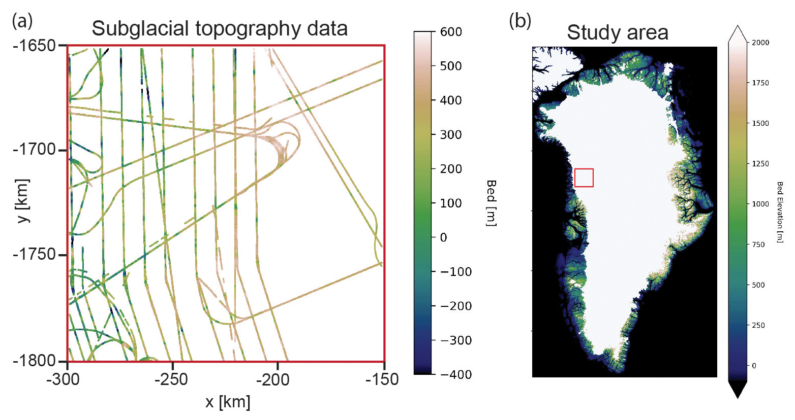
Figure 1 Ice-penetrating radar topography data for test region. The coordinates are shown in a polar stereographic projection.

3 Interpolation with existing geostatistical tools

It was our original intent to test existing Python interpolation functions from PyKrige, GSTools, and GeostatsPy on the aforementioned bed elevation data set in order to establish a baseline level of performance for comparison with GStatSim. However, the PyKrige and GSTools kriging and conditional simulation routines crash when applied to our data set due to the high random access memory (RAM) consumption. We are also unable to produce a simulation result using GeostatsPy due to a “singular matrix” error, which generally indicates that there is some sort of numerical instability. We discuss these limitations in more detail in Sect. 7. Only the GeostatsPy kriging function is successfully applied to this data set. The GeostatsPy kriging implementation and results are described in Sect. 4.3.3.

4 GStatSim functions and implementation

GStatSim can be used with Python 3.0–3.10 and relies on commonly used packages such as scipy (Virtanen et al., 2020), numpy (Harris et al., 2020), pandas (McKinney, 2010), and scikit-learn (Pedregosa et al., 2011). This ensures that GStatSim is easy to use in different computing environments. The source code is written in accordance with PEP8 standards (Van Rossum et al., 2001), making it interpretable and easy to modify.

4.1 Data initialization

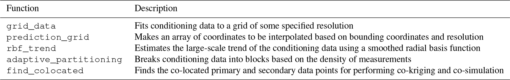
Prior to performing any geostatistical analysis, we fit the bed elevation data to a 1 km resolution grid using the GStatSim grid_data function which averages values within each grid cell. We do this because the interpolation examples shown in this paper use a 1 km resolution. In this way, the spatial statistics of the data will be compatible with the interpolation grid. This gridded data set has 3650 data points. In order to satisfy the Gaussian assumptions of our interpolation functions, we convert our data to a standard Gaussian distribution using the scikit-learn QuantileTransformer function. This step converts the data to a standard Gaussian distribution (mean =0, variance =1), shown in Fig. 2. It is not strictly necessary for data to be Gaussian when using GStatSim. However, the interpolation results will be more robust if a Gaussian distribution is used.

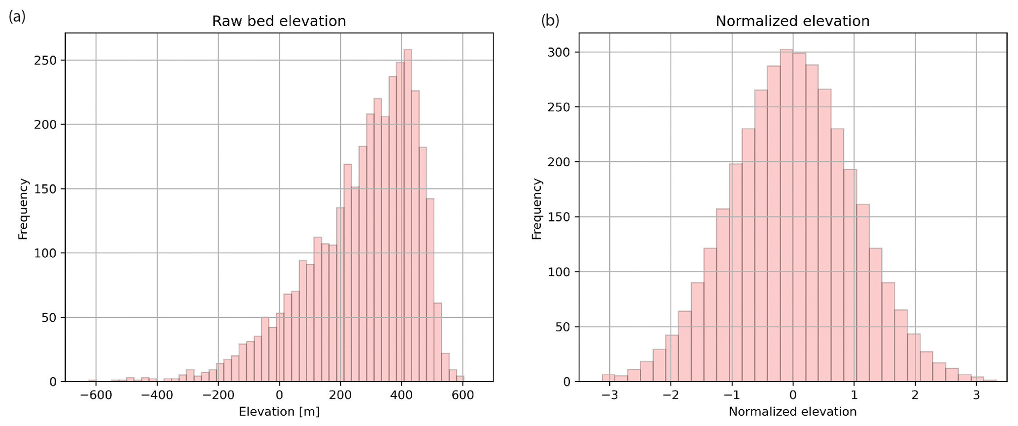
Figure 2 (a) Original data distribution. (b) Transformed data with a standard Gaussian distribution.

Table 1 GStatSim interpolation functions.

Table 2 GStatSim accessory functions.

4.2 Variogram calculation and modeling with SciKit-GStat

The interpolation functions in GStatSim rely on the variogram, which describes spatial statistics by quantifying the covariance between data points as a function of their separation distance or lag (Matheron, 1963). The experimental variogram γ(h) is defined as the averaged squared differences of data points separated by a lag distance h:

$$\begin{array}{}\text{(1)}& \mathit{\gamma }\left(h\right)={\displaystyle \frac{\mathrm{1}}{\mathrm{2}N\left(h\right)}}\sum _{\mathit{\alpha }=\mathrm{1}}^N\left(Z\right(u_{\mathit{\alpha }})-Z(u_{\mathit{\alpha }}+h){)}^{\mathrm{2}},\end{array}$$

where Z is a variable, u is a spatial location, and N(h) is the number of pairs of data points for a lag h. Typically, the variance increases with lag distance until a threshold is reached where measurements are no longer spatially correlated. This threshold is called the sill, which is, in theory, equal to 1 for normalized data sets. The lag distance where the variogram reaches the sill is called the range.

GStatSim does not include variogram estimation tools as there are already existing resources (e.g., SciKit-GStat). Our interpolation functions are designed to be integrated with outside variogram modeling tools. We perform our variogram analysis with the SciKit-GStat functions, which offer robust tools for variogram estimation and modeling. We compute both the isotropic and anisotropic variograms. The anisotropic variogram computes the variogram for different angles from horizontal. Figure 3 shows that the data do not contain significant anisotropy. While the anisotropic variograms do exhibit some disagreement at lags greater than ∼35 km, these differences can be attributed to regional trends in the topography. Additionally, the first part of the variogram with small lags is more important than the tail distributions when it comes to calculating the kriging weights used for interpolation. As such, only the isotropic variogram is used for the variogram modeling analysis.

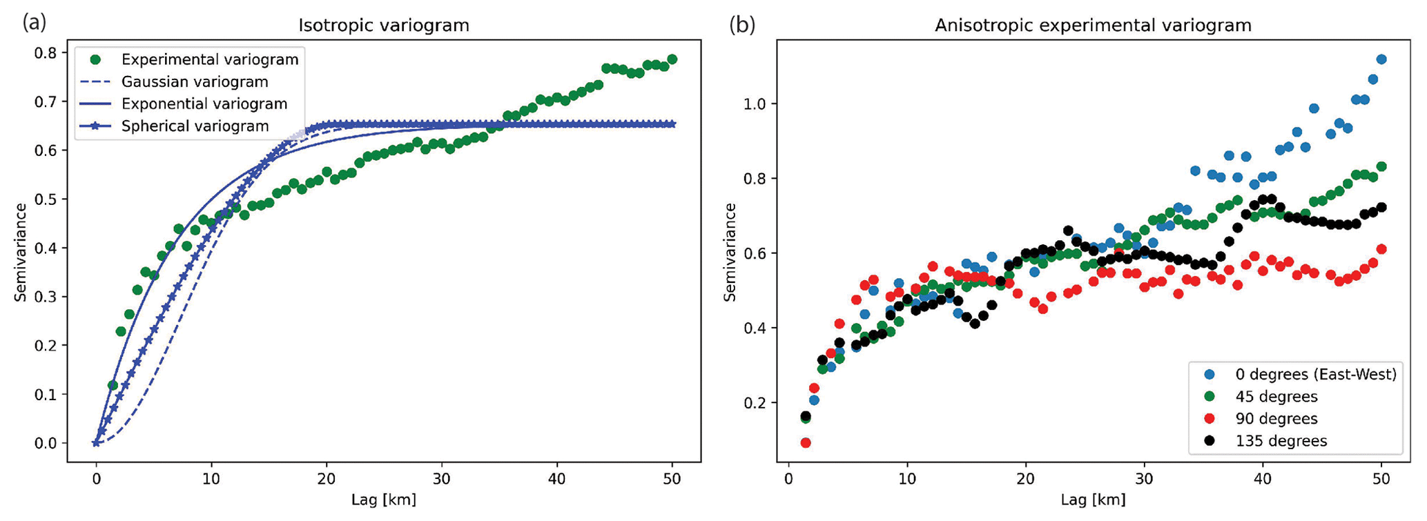
Figure 3 (a) Isotropic experimental variogram and variogram model. (b) Anisotropic variogram.

In order to use the variogram for interpolation, a variogram model must be fit to the experimental variogram. GStatSim can currently accommodate exponential, Gaussian, and spherical variogram model types. The exponential model is as follows:

$$\begin{array}{}\text{(2)}& {\mathit{\gamma }}_{\exp }\left(h\right)=\left\{\begin{array}{lll}\mathrm{0}& \text{if}& h=\mathrm{0}\\ b+(C_{\mathrm{0}}-b)\left[\mathrm{1}-e^{-\frac{\mathrm{3}h}{a}}\right]& \text{if}& h>\mathrm{0}\end{array},\right.\end{array}$$

where a is the range parameter, C₀ is the sill, and b is the nugget. The nugget describes the variance at near-zero lags, which is often the result of measurement error. In most cases, the nugget is zero. The Gaussian model is

$$\begin{array}{}\text{(3)}& {\mathit{\gamma }}_{\text{Gauss}}\left(h\right)=\left\{\begin{array}{lll}\mathrm{0}& \text{if}& h=\mathrm{0}\\ b+(C_{\mathrm{0}}-b)\left[\mathrm{1}-e^{-\frac{\mathrm{3}{h}^{\mathrm{2}}}{a^{\mathrm{2}}}}\right]& \text{if}& h>\mathrm{0}\end{array},\right.\end{array}$$

and the spherical model is

$$\begin{array}{}\text{(4)}& \begin{array}{rl}& {\mathit{\gamma }}_{\text{sph}}\left(h\right)\\ & =\left\{\begin{array}{ll}\mathrm{0}& \text{if}h=\mathrm{0}\\ b+(C_{\mathrm{0}}-b)\left(\mathrm{1.5}\cdot \frac{h}{a}-\mathrm{0.5}\cdot \frac{h^{\mathrm{3}}}{a^{\mathrm{3}}}\right)& \text{if}\mathrm{0}<h\le a\\ C_{\mathrm{0}}& \text{if}h>a\end{array}.\right.\end{array}\end{array}$$

See Chiles and Delfiner (2009) for a detailed description of these models. In practice, variogram model parameters are often selected manually, though SciKit-GStat also offers automatic variogram modeling tools. Using these tools, we fit each of these model types to the experimental variogram, shown in Fig. 3a. A visual inspection of Fig. 3a shows that the exponential variogram model produces the best fit. As such, we use this model type for the topography interpolations shown in this paper. The exponential model has a nugget of 0, a range of 31.9 km, and a sill of 0.7. Geostatistical interpolations can be sensitive to the methods and parameters used to compute and model variograms. As such, we recommend referring to the SciKit-GStat documentation for best practices and considerations when conducting variogram analysis. The effect of different variogram models on interpolations is described in Sect. 4.5.

4.3 Kriging

Kriging is used to produce deterministic interpolations of a spatial variable, where the goal is to minimize estimation variance (e.g., Matheron, 1963; Cressie, 1990). For a spatial variable Z, kriging models the residuals Z^* from a mean m:

$$\begin{array}{}\text{(5)}& Z^{*}\left(u_{\mathit{\alpha }}\right)=Z\left(u_{\mathit{\alpha }}\right)-m\left(u_{\mathit{\alpha }}\right).\end{array}$$

In cases where the mean is constant, m is treated as a global mean. Each interpolated value Z^* at a location u is the weighted sum of neighboring measurements:

$$\begin{array}{}\text{(6)}& Z^{*}\left(u_{\mathrm{0}}\right)=\sum _{\mathit{\alpha }}^N{\mathit{\lambda }}_{\mathit{\alpha }}Z\left(u_{\mathit{\alpha }}\right),\end{array}$$

where λ_α are the weights on the N data points. These weights account for the variability in the measurements, their proximity to each other and the node being estimated, and the redundancy between nearby measurements. Specifically, the weights are determined by solving the kriging system of equations which, for a system with three data points, would look like

$$\begin{array}{}\text{(7)}& \begin{array}{rl}& \left[\begin{array}{ccc}C(u_{\mathrm{1}}-u_{\mathrm{1}})& C(u_{\mathrm{1}}-u_{\mathrm{2}})& C(u_{\mathrm{1}}-u_{\mathrm{3}})\\ C(u_{\mathrm{2}}-u_{\mathrm{1}})& C(u_{\mathrm{2}}-u_{\mathrm{2}})& C(u_{\mathrm{2}}-u_{\mathrm{3}})\\ C(u_{\mathrm{3}}-u_{\mathrm{1}})& C(u_{\mathrm{3}}-u_{\mathrm{2}})& C(u_{\mathrm{3}}-u_{\mathrm{3}})\end{array}\right]\left[\begin{array}{c}{\mathit{\lambda }}_{\mathrm{1}}\\ {\mathit{\lambda }}_{\mathrm{2}}\\ {\mathit{\lambda }}_{\mathrm{3}}\end{array}\right]\\ & =\left[\begin{array}{c}C(u_{\mathrm{0}}-u_{\mathrm{1}})\\ C(u_{\mathrm{0}}-u_{\mathrm{2}})\\ C(u_{\mathrm{0}}-u_{\mathrm{3}})\end{array}\right]\end{array},\end{array}$$

which can be abbreviated to

$$\begin{array}{}\text{(8)}& \mathbf{C}\mathit{\lambda }=\mathit{c},\end{array}$$

where C describes the covariance between pairs of data points, and c describes the covariance between each data point and the location that is being estimated, u₀. Note that the covariance is linked to the variogram:

$$\begin{array}{}\text{(9)}& C\left(h\right)=C\left(\mathrm{0}\right)-\mathit{\gamma }\left(h\right),\end{array}$$

where C(0) is the variance of the data. We use the modeled variogram parameters determined in Sect. 4.2.

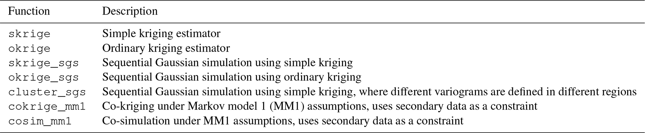
GStatSim contains functions for both simple and ordinary kriging. With simple kriging, it is assumed that the mean is a constant, known parameter defined by the mean of the data. For data that have undergone a normal score transformation, the mean is 0. For ordinary kriging, the mean is estimated implicitly within a search neighborhood around the coordinate being estimated, and simple kriging is applied to the residuals. This makes ordinary kriging more robust to spatial trends. The ordinary kriging weight estimation procedure is modified from Eq. (7) to

$$\begin{array}{}\text{(10)}& \begin{array}{rl}& \left[\begin{array}{cccc}C(u_{\mathrm{1}}-u_{\mathrm{1}})& C(u_{\mathrm{1}}-u_{\mathrm{2}})& C(u_{\mathrm{1}}-u_{\mathrm{3}})& \mathrm{1}\\ C(u_{\mathrm{2}}-u_{\mathrm{1}})& C(u_{\mathrm{2}}-u_{\mathrm{2}})& C(u_{\mathrm{2}}-u_{\mathrm{3}})& \mathrm{1}\\ C(u_{\mathrm{3}}-u_{\mathrm{1}})& C(u_{\mathrm{3}}-u_{\mathrm{2}})& C(u_{\mathrm{3}}-u_{\mathrm{3}})& \mathrm{1}\\ \mathrm{1}& \mathrm{1}& \mathrm{1}& \mathrm{0}\end{array}\right]\left[\begin{array}{c}{\mathit{\lambda }}_{\mathrm{1}}\\ {\mathit{\lambda }}_{\mathrm{2}}\\ {\mathit{\lambda }}_{\mathrm{3}}\\ \mathit{\mu }\end{array}\right]\\ & =\left[\begin{array}{c}C(u_{\mathrm{0}}-u_{\mathrm{1}})\\ C(u_{\mathrm{0}}-u_{\mathrm{2}})\\ C(u_{\mathrm{0}}-u_{\mathrm{3}})\\ \mathrm{1}\end{array}\right]\end{array},\end{array}$$

where μ is a Lagrange multiplier. The covariance function is also used to compute the uncertainty, or variance, at each location. The variance of an estimate at location u₀, ${\mathit{\sigma }}_E^{\mathrm{2}}\left(u_{\mathrm{0}}\right)$ is defined as

$$\begin{array}{}\text{(11)}& {\mathit{\sigma }}_E^{\mathrm{2}}\left(u_{\mathrm{0}}\right)=C\left(\mathrm{0}\right)-\sum _{\mathit{\alpha }}^N{\mathit{\lambda }}_{\mathit{\alpha }}C(u_{\mathrm{0}}-u_{\mathit{\alpha }}).\end{array}$$

The ability of kriging to quantify uncertainty is a major advantage of this method over other deterministic interpolation methods such as spline interpolation.

4.3.1 Nearest-neighbor octant search

In practice, the covariance matrices in Eqs. (7) and (10), C and c, used to determine kriging weights typically do not use every value in the conditioning data. Instead, it is conventional to use the N nearest neighbors, where N is the number of conditioning nodes (e.g., Pyrcz et al., 2021). This significantly reduces the size of the covariance matrix and ensures that estimates are made using only relevant information. However, the nearest-neighbor approach can be problematic when the conditioning data are unevenly spatially distributed. In the ice-penetrating radar example, measurements are sampled densely along flight lines but are entirely absent in between lines. This means that the N nearest neighbors of a coordinate next to a flight line could all be on one side, yielding lopsided conditioning data (Fig. 4). This lopsidedness would produce skewed estimates. To avoid this bias, our interpolation algorithms use a nearest-neighbor octant search (e.g., Pebesma, 2004), where the N neighbors are divided amongst the eight different octants of the coordinate plane (Fig. 4). This ensures that the conditioning data include values on all sides of the node being estimated. The ability of the nearest-neighbor octant search to produce a balanced conditioning data set is important for producing high-quality estimates, particularly for remote sensing data sets where the measurement density is often non-uniform. We note that the primary drawback of this approach is that it increases the algorithm runtime.

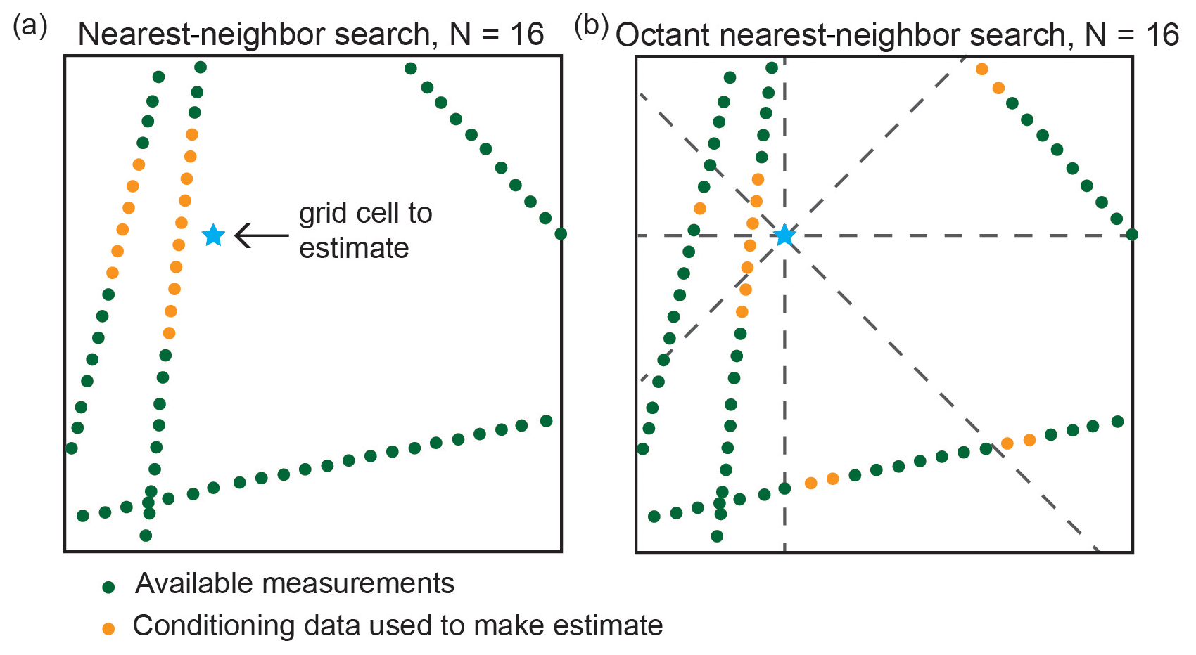
Figure 4 When measurements are gathered along line surveys, a simple nearest-neighbor search (a) may result in estimates being skewed towards values on one side. The octant nearest-neighbor search (b) used in GStatSim ensures that the conditioning data surround the coordinate being estimated, which minimizes this bias in interpolations.

4.3.2 Covariance matrix inversion

According to Eq. (8), solving for the kriging weights λ requires the inversion of the covariance matrix C:

$$\begin{array}{}\text{(12)}& \mathit{\lambda }={\mathbf{C}}^{-\mathbf{1}}\mathbf{c}.\end{array}$$

However, C is not always a positive definite matrix, meaning that C⁻¹ cannot be computed. This is especially common for complex scenarios such as ice-penetrating radar data sets which often contain overlapping and conflicting measurements. The matrix singularity issue can be resolved by computing the pseudo-inverse, C⁺, instead. However the pseudo-inverse requires a time-consuming singular value decomposition with a runtime that scales by O(n³) with data input size, making it an impractical choice for applications with large data sets. For improved performance, we use the scipy.linalg.lstsq function, which computes the least-squares solution to the equation Ax=b. Solving for the weights with lstsq instead of computing the matrix inversion directly lends greater numerical stability to the interpolation functions. Therefore, all functions in GStatSim involving covariance matrix inversions are implemented using lstsq.

4.3.3 Kriging implementation and results

We implement simple kriging and ordinary kriging using the GStatSim skrige and okrige functions, respectively. The input parameters for these functions are the conditioning data, search radius, number of conditioning points, variogram parameters, and a list of coordinates that describe the prediction grid. We use a search radius of 50 km and 100 conditioning points. For convenience, GStatSim includes a prediction_grid function that automatically generates a list of coordinates defined by the minimum and maximum coordinate extents and the grid cell resolution. After GStatSim interpolation is applied, the kriging estimates are back-transformed using the scikit-learn QuantileTransformer function so that the original data distribution is recovered. For comparison, we also perform simple kriging using the GeostatsPy kb2d function.

The GStatSim kriging results (Fig. 5) show that the right side of the ordinary kriging estimate has a slightly higher (∼ tens of meters) elevation than the simple kriging estimate. This is because ordinary kriging does not assume that the mean is constant. The GStatSim and GeostatsPy simple kriging estimates are visually similar but differ by tens of meters throughout the domain. The black arrows in Fig. 5c and f highlight a visible seam in the GeostatsPy interpolation. This seam is located along grid cells that are equidistant from conditioning lines and may be the result of using a simple nearest-neighbor search (Fig. 4).

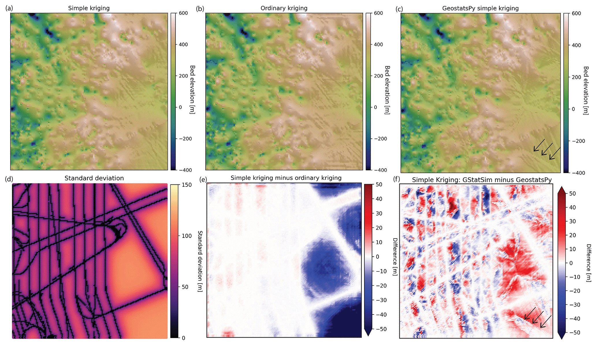
Figure 5 (a) Simple kriging and (b) ordinary kriging interpolations using GStatSim. (c) Simple kriging interpolation using GeostatsPy. (d) Standard deviation for the simple kriging estimate from panel (a). (e) Difference between simple and ordinary kriging. (f) Difference between GStatSim and GeostatsPy simple kriging. The black arrows highlight an artifact in the GeostatsPy interpolation that is likely caused by using a simple nearest-neighbor search (Fig. 4).

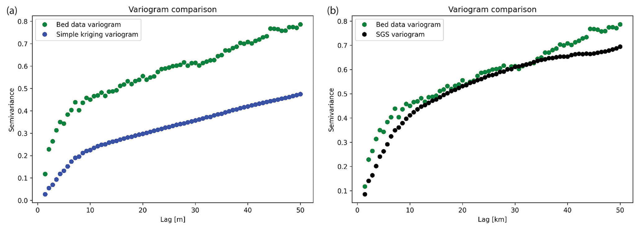
To investigate the spatial statistics of kriging interpolation, we compute the variogram for the GStatSim simple kriging estimate. The resulting variogram, shown in Fig. 6a, has substantially lower variances than the experimental variogram derived from the data. This difference highlights an important limitation of kriging interpolation: the variogram is not reproduced, making the interpolated values smoother than observations.

Figure 6 (a) Variogram for simple kriging estimate from Fig. 5a. (b) Variogram for SGS realization no. 1.

4.4 Sequential Gaussian simulation

In contrast to kriging, sequential Gaussian simulation (SGS) is designed to preserve the variance of observations. SGS is the stochastic alternative to kriging. In contrast to kriging where the objective is to optimize local accuracy, SGS is used to generate multiple realizations that reproduce the variogram statistics (e.g., Deutsch and Journel, 1992). The implementation of SGS, described in Fig. 7, is the following:

1. Define a random simulation order in which to visit each node.

2. At each node u, use kriging to estimate the mean Z^*(u) and variance ${\mathit{\sigma }}_E^{\mathrm{2}}\left(u\right)$.

3. Randomly sample from the Gaussian distribution defined by Z^*(u) and ${\mathit{\sigma }}_E^{\mathrm{2}}\left(u\right)$. This becomes the simulated value at that node.

4. Proceed to the next node and repeat steps 2 and 3 until all nodes have been simulated.

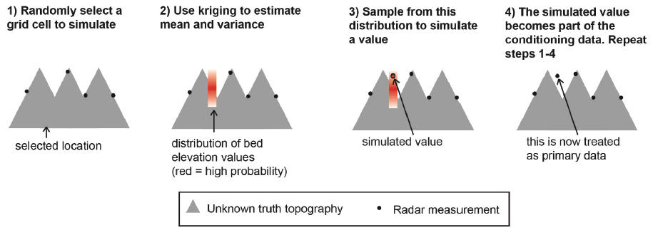
Figure 7 Schematic of SGS. This figure is modified from MacKie et al. (2021), which was published under a Creative Commons Attribution license (https://creativecommons.org/licenses/by/4.0/, last access: 1 May 2023).

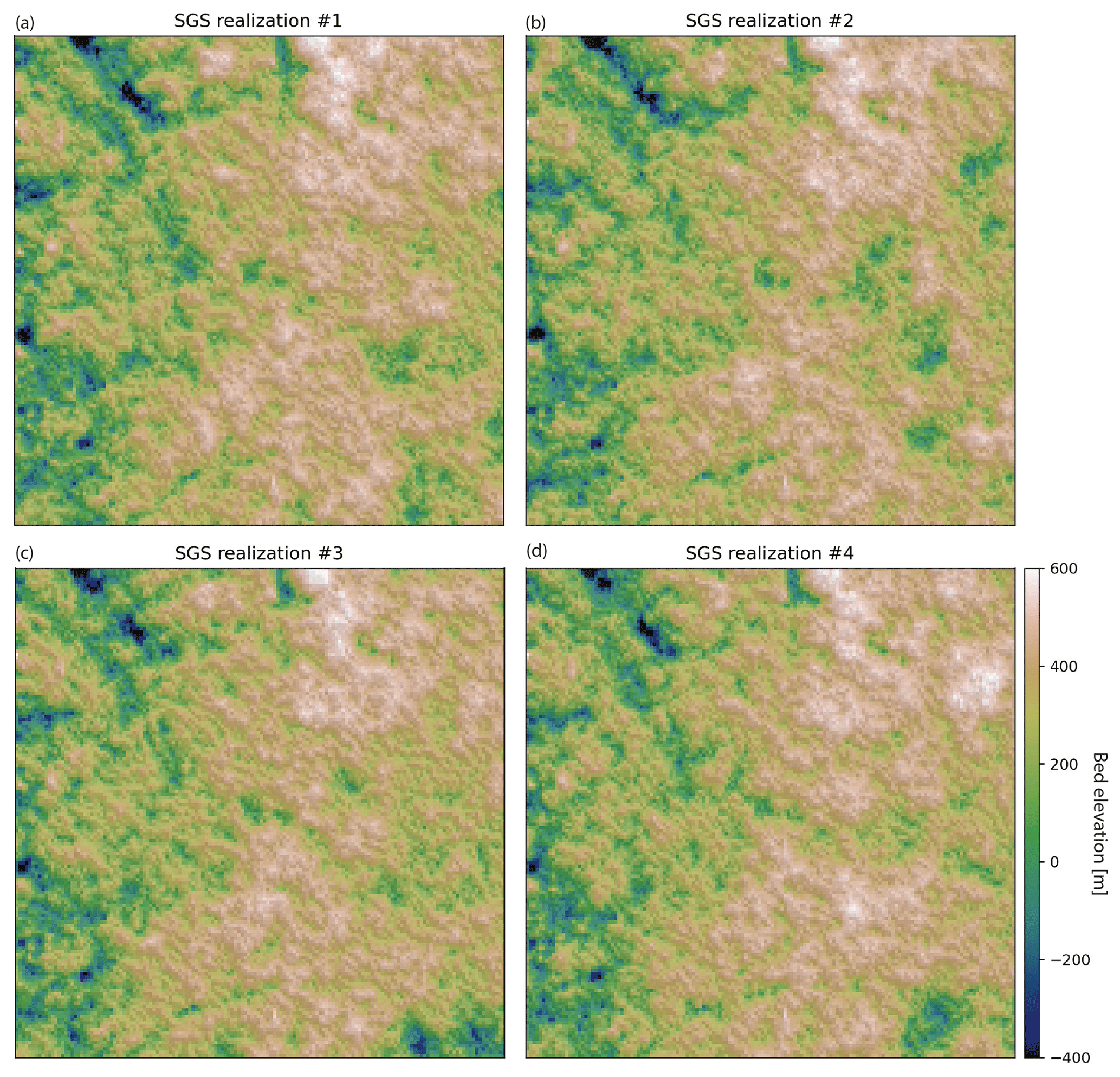
GStatSim has two different SGS functions, okrige_sgs and skrige_sgs, which use ordinary kriging and simple kriging for step 2, respectively. The results are unlikely to differ significantly between these two methods, but okrige_sgs may be more robust when large-scale trends are present. The input parameters are the same as those used for the skrige and okrige functions. We simulate four realizations using okrige_sgs using the same input parameters as in Sect. 4.3.3. To evaluate the ability of SGS to reproduce the spatial statistics of observations, we compute the variogram for realization no. 1 (Fig. 6). The variogram of the simulated topography matches the variogram of observations. The realizations are shown in Fig. 8. Each realization matches the conditioning data and represents an equally probable solution.

Figure 8 (a–d) SGS realizations generated with okrige_SGS.

4.5 Interpolation with different variogram models

GStatSim can perform interpolations using the exponential, Gaussian, or spherical variogram models, as described in Sect. 4.2. In this section, we demonstrate how interpolations differ when using different variogram model types. We generate a synthetic conditioning data set of 100 points using the unconditional Gaussian field tools in GSTools (Fig. 9a). We use a variance of 2 and length scale of 8. While the true variogram for the synthetic data is Gaussian, we perform interpolations using different variogram models for demonstration purposes. We compute the experimental variogram and fit Gaussian, exponential, and spherical variogram models (Fig. 9b). Then we perform both simple kriging interpolation and SGS with each variogram model. The results, shown in Fig. 9, show that the Gaussian model produces the SGS realization with the smoothest spatial structure and lowest kriging variance. The exponential model produces the roughest SGS topography and highest kriging variance, and the spherical model falls in the middle. These different model types allow GStatSim to accommodate different types of spatial structures.

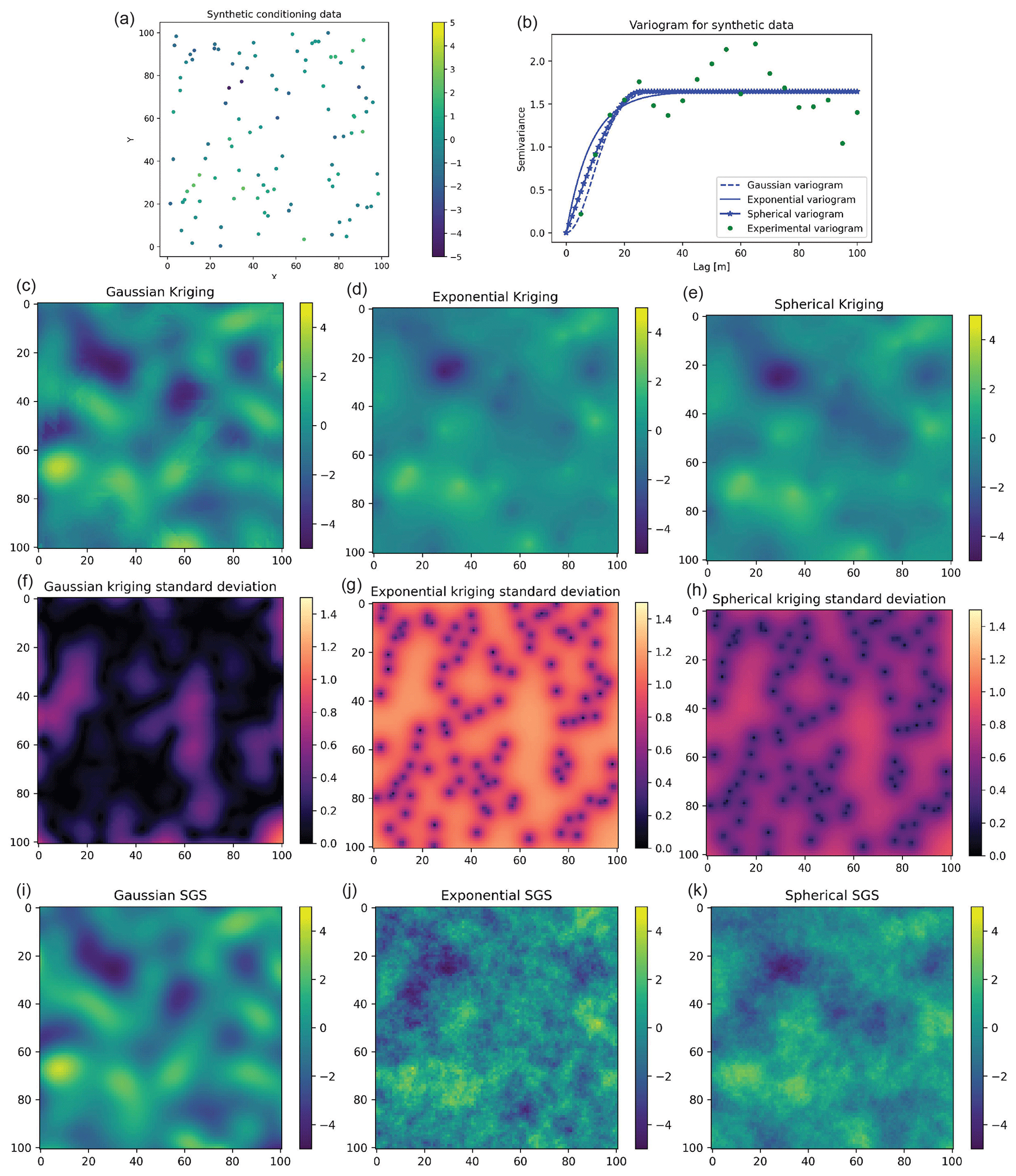
Figure 9 Interpolation comparison using different variogram models. Synthetic conditioning data (a), variograms (b), kriging interpolation (c–e), kriging uncertainty (f–h), and SGS (i–k).

4.6 Interpolation with anisotropy

Geologic phenomena frequently exhibit anisotropy in their spatial statistics. For example, preferential erosion can cause subglacial topography to be smoother in the direction that is parallel to ice flow (MacKie et al., 2021). The GStatSim interpolation functions can account for this anisotropy by accepting major and minor range parameters. The major range is the range of the variogram in the smoothest (major) direction, and the minor range is the range of the variogram in the minor direction, which is orthogonal to the major direction. Not all pairs of data points are oriented along the major or minor orientations, so the range is treated as the radius of a rotated ellipse where the major and minor ranges are the lengths of each axis, and the degree of rotation is determined by the angle of anisotropy. The major angle orientation is defined as the angle from zero (horizontal) of the major direction. In practice, these parameters can be determined by modeling the variogram in multiple directions and determining the major angle through visual inspection.

To demonstrate the implementation of interpolation with anisotropy, we perform simple kriging and SGS with anisotropy for angles of 0 and 60^∘. We use the modeled variogram parameters from previous sections (nugget =0, range =31.9 km, sill =0.7). We use 31.9 km as the minor range and set the major range to be 15 km greater than the minor range for exaggerated effect. These interpolations (Fig. 10) have clearly visible anisotropy.

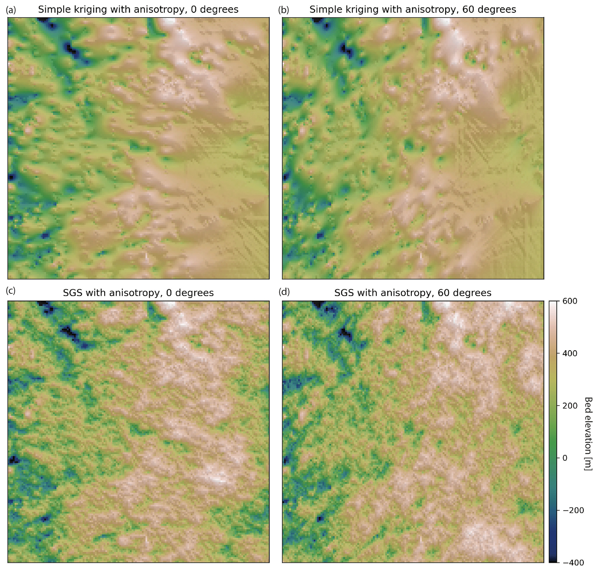
Figure 10 (a) Simple kriging with anisotropy at 0^∘. (b) Simple kriging with anisotropy at 60^∘. (c) SGS with anisotropy at 0^∘. (d) SGS with anisotropy at 60^∘.

4.7 Mean non-stationarity

Data sets often contain variations in spatial statistics, a condition known as non-stationarity. Mean non-stationarity occurs in the presence of a large-scale trend or systematic changes across a study area. While ordinary kriging can accommodate variations in the mean, to some extent, it does not extrapolate well (Journel and Rossi, 1989). For this reason, it is sometimes convenient to detrend the data prior to variogram modeling and interpolation. This approach is known as kriging (or SGS) with a trend or universal kriging. Detrending has the additional advantage of producing residual data that more closely represent a random Gaussian process, which makes the variogram modeling more robust. In contrast, data with a strong trend can yield an experimental variogram that never reaches an obvious sill, making it difficult to fit a variogram model.

Here we demonstrate kriging and SGS with a trend (Fig. 11). This is achieved by the following:

1. Estimate the trend.

2. Subtract the trend from the data to obtain residual measurements.

3. Apply a normal score transformation to the residual data.

4. Conduct a variogram analysis on the transformed residual measurements.

5. Interpolate the residuals.

6. Back-transform the interpolation to recover the original data distribution.

7. Add the back-transformed interpolation to the trend.

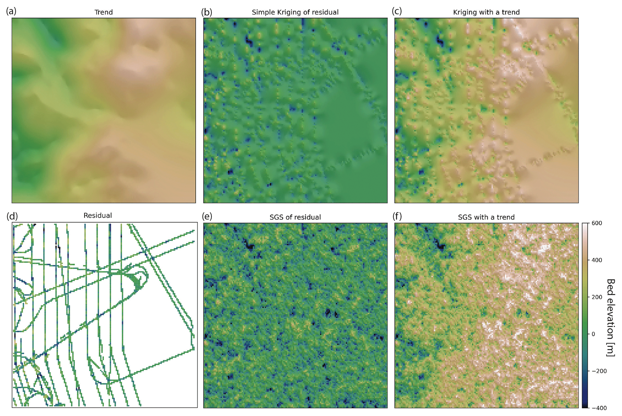
Figure 11 (a) Trend estimate. (b) Simple kriging of detrended data. (c) The simple kriging estimate from panel (b) added to the trend from panel (a). (d) The residual bed elevation data after the trend is subtracted from the data. (e) SGS applied to the detrended data. (f) The SGS interpolation from panel (e) added to the trend from panel (a).

While it is common practice to estimate the trend by fitting a linear or polynomial function to the data (e.g., Neven et al., 2021), determining higher-order polynomial models for complex landscapes can be difficult. Instead, we estimate the trend using a radial basis function (RBF), which is a function that changes with distance from a location, such as a thin-plate spline or Gaussian function. RBFs measure the distance between input values and a center point, assigns weights based on these distances, and combines these weights to produce an output value (Broomhead and Lowe, 1988). The RBF trend estimation was implemented using the GStatSim rbf_trend function, which relies on the scipy RBF implementation. rbf_trend uses a multiquadric kernel as its RBF, which is known for its high accuracy and flexibility (Franke, 1982; Sarra and Kansa, 2009). The rbf_trend function input parameters are the conditioning data, the grid cell resolution, and a smoothing factor. The smoothing factor ensures that the trend is not overfitting to measurements. The smoothing parameter should be at least as large as the largest data gap. We use a smoothing factor of 100 km.

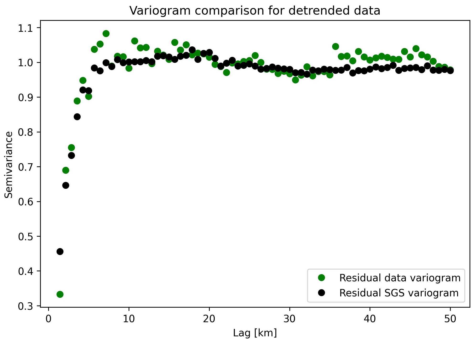
To evaluate the performance of the detrended SGS approach, we compute the experimental variogram for residual data (Fig. 11d) and the residual SGS (Fig. 11e). The variograms, shown in Fig. 12, show close agreement between the spatial statistics of the residual measurements and simulation. Note that both variograms reach a sill of 1 in contrast to the variogram for the data without detrending (Fig. 6). According to the theoretical definition of the variogram (Eq. 2), data with a standard Gaussian distribution should reach a sill of 1. As such, the detrended data can often be better suited to variogram-based interpolation.

Figure 12 Variogram for detrended data from Fig. 11d and simulation of trend from Fig. 11e. These variograms have a sill of 1, which is the theoretical sill for standard Gaussian data.

4.8 Variogram non-stationarity

Variogram non-stationarity describes the condition when the variogram statistics vary throughout a domain. For example, the topographic roughness varies throughout Greenland (Cooper et al., 2019). To handle these cases, GStatSim includes a cluster_sgs function where the user can assign different variograms to different areas. It is implemented by partitioning the data into different clusters and then computing the variogram for each cluster. To simulate a grid cell,

1. choose a random grid cell;

2. find the nearest-neighbor value and look up the cluster number of the nearest-neighbor point;

3. using the variogram parameters associated with the cluster of the nearest point, simulate a value with SGS;

4. assign the nearest-neighbor cluster number to the simulated value;

5. repeat until each grid cell is simulated.

This process ensures that the boundaries between different clusters vary for each realization. cluster_sgs takes the same inputs as SGS, as well as the cluster numbers for each data point and a data frame with the variogram parameters for each cluster. Users can use any method they like to partition the data into different clusters. In the next two subsections, we outline two approaches.

4.8.1 K-means clustering approach

One of the simplest ways to cluster data is with k-means clustering, where the data are partitioned into k clusters such that the average squared sum of distances from the center within each cluster is minimized. We apply k-means clustering to the conditioning data and determine three clusters based on the coordinates and bed elevation (Fig. 13a). The justification for using these parameters is that data points that are geographically close to each other and have similar elevation values should have similar spatial statistics. We use a k of 3, which was chosen arbitrarily for demonstration purposes. In real applications, external information or domain expertise may be used to inform the clustering decision.

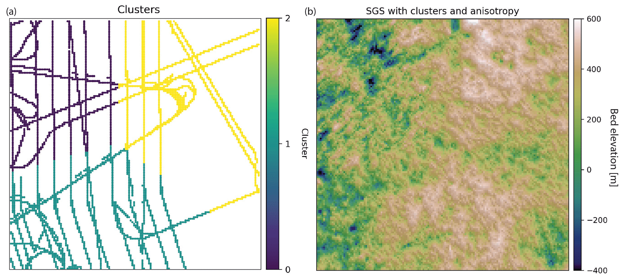
Figure 13 (a) K-means clustering of conditioning data. (b) SGS using different variogram parameters for each cluster.

We apply the variogram analysis to the data in each cluster separately using the procedure described in Sect. 4.2. To make the differences between clusters more pronounced, we manually modify several of the variogram parameters to exaggerate the differences in spatial statistics for visualization purposes. Clusters 0 and 2 are assigned angles for anisotropy (45^∘ for Cluster 0 and 90^∘ for Cluster 2). The minor ranges for Clusters 0 and 2 are assigned based on the automatic variogram modeling. The major ranges are set by adding 15 km to the minor ranges. Cluster 1 is given a sill of 0.6, and Clusters 0 and 2 are assigned sills equal to 1. The cluster_sgs simulation using these parameters produces visible differences in spatial statistics throughout the domain. For example, the anisotropy is clearly visible in the region defined by Cluster 0 (Fig. 13b). Despite the extreme differences in parameters used for each cluster, the cluster boundaries do not have artifacts or inconsistencies.

4.8.2 Adaptive partitioning

The k-means clustering approach described above provides a simple approach to partitioning the data, but the decision boundaries can seem arbitrary and result in clusters with widely varying sample counts. To overcome these challenges we present a recursive implementation of a divisive, density-based clustering approach we call adaptive partitioning. A similar approach was used in Yin et al. (2022). The algorithm begins by treating the data set as a single cluster and quartering this cluster into four rectangles of equal area. For each subsequent cluster, the areal extent of the cluster continues to be quartered until the number of data samples contained within the cluster is below the maximum number of samples allowed or the minimum cluster size has been reached. GStatSim implements this as a fully recursive function named adaptive_partitioning with primary parameters max_points, which controls the maximum points allowed in a cluster, and min_length, which controls the minimum side length of a cluster. It may take tuning of these two parameters to produce a desirable partitioning, including adjusting max_points to create clusters of adequate sizes given the measurement density; min_length should be greater than the expected variogram range to ensure that there are sufficient data to accurately model the variogram parameters. Figure 14a shows the clusters resulting from adaptive_partitioning with max_points of 800 and min_length of 25 km.

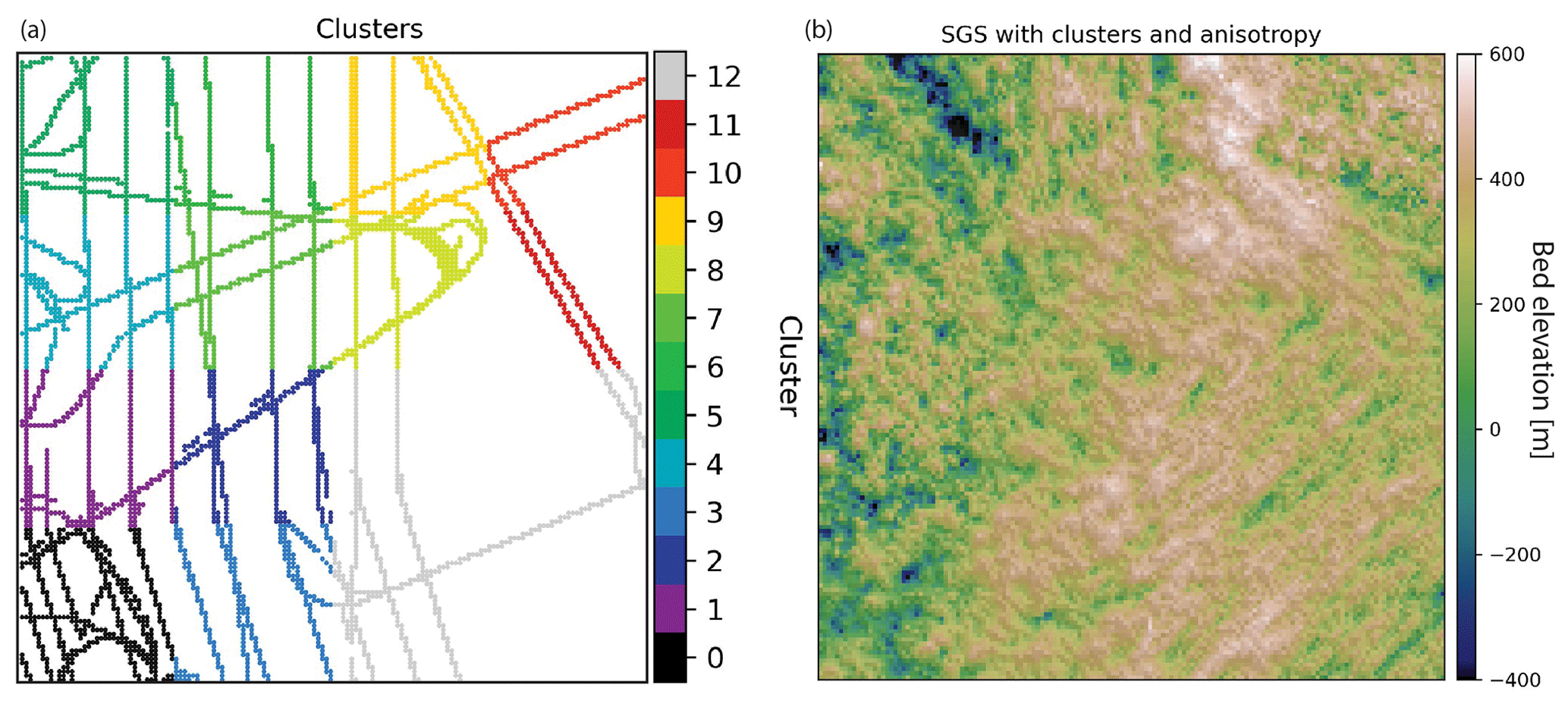
Figure 14 (a) Clusters derived from density-based adaptive partitioning function. (b) SGS using a different variogram in each cluster.

The variogram parameters for each cluster are modeled automatically and then modified to show exaggerated differences between clusters. Cluster 1 is modified to have a sill of 0.6. Clusters 6 and 12 are given 90 and 45^∘ directions of anisotropy, respectively, with major ranges that are determined by adding 15 km to the modeled range. These regional differences in variogram parameters are apparent in the resulting simulation in Fig. 14.

4.9 Co-kriging and co-simulation

Secondary information can be integrated into interpolations via co-kriging and co-simulation, where a well-sampled secondary variable is used to constrain the interpolation of a sparsely sampled primary variable. For example, if the ice surface elevation (Fig. 15a) is found to be correlated with the subglacial bed elevation, then the ice surface can be used to improve the interpolation. We note that the ice surface and subglacial topography are unlikely to be linearly related (Ng et al., 2018); this example is merely intended to demonstrate the usage of our co-kriging and co-simulation tools. In theory, co-kriging and co-simulation are implemented by modeling the variogram for each variable and a cross-variogram that describes the covariation between the variables. In practice, the full co-kriging system of equations is difficult to solve, so approximations are used instead (Almeida and Journel, 1994; Journel, 1999).

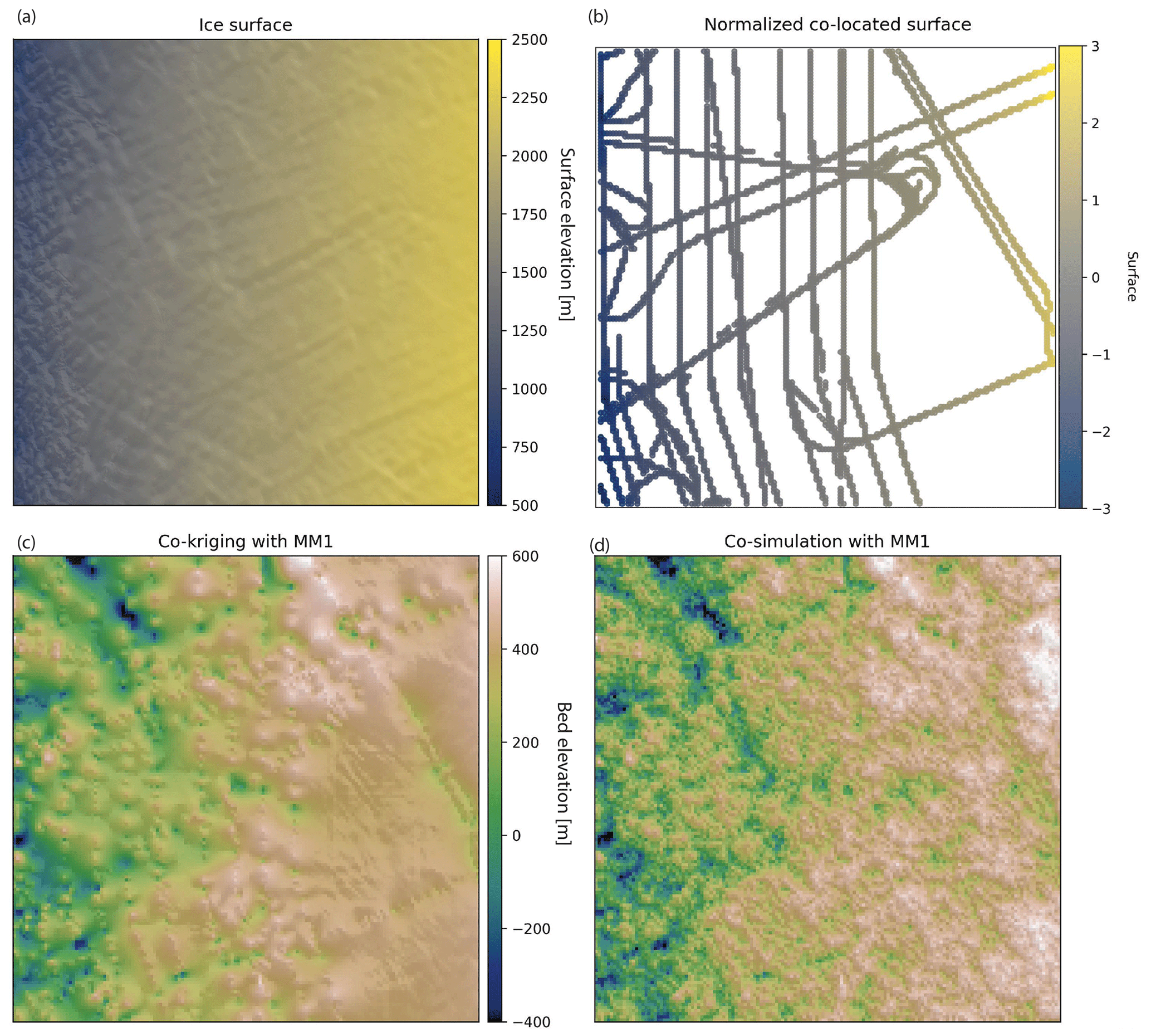
Figure 15 (a) Ice surface elevation data. (b) Normalized ice surface elevation measurements that are co-located with radar measurements. (c) Co-kriging interpolation. (d) Co-simulation.

While there are several different ways to implement co-kriging (Journel, 1999), GStatSim only includes functions for co-located co-kriging under Markov model 1 (MM1) assumptions, as described by Almeida and Journel (1994). This version was chosen for its simplicity; expert geostatistical knowledge is not needed to use this algorithm. Co-located co-kriging means that an estimate is made using only the secondary data point that is co-located with, or at the same location as, the grid cell being estimated. This significantly reduces the number of conditioning data points that are used to estimate each grid cell. Co-kriging with MM1 approximates the cross-variogram through a Markov assumption of conditional independence. It is assumed that a secondary data variable Z₂ at a location u is conditionally independent of the primary variable Z₁ at a location of u^′, given Z₁(u). u^′ refers to a spatial location that is not u. This statement of conditional independence is written as

$$\begin{array}{}\text{(13)}& \begin{array}{rl}E\left(Z_{\mathrm{2}}\right(u\left)\right|Z_{\mathrm{1}}\left(u\right)& =z_{\mathrm{1}},Z_{\mathrm{1}}\left(u^{\prime }\right)=z_{\mathrm{1}}\left(u^{\prime }\right))\\ & =E\left(Z_{\mathrm{2}}\right(u\left)\right|Z_{\mathrm{1}}\left(u\right)=z_{\mathrm{1}}),\end{array}\end{array}$$

where E refers to the expected value. In the geostatistical community, this Markov assumption is referred to as Markov model 1 (Almeida and Journel, 1994). See Journel (1999) and Shmaryan and Journel (1999) for other co-kriging models. In the case where the ice surface elevation is used as a secondary constraint, MM1 means that the expected value of the ice surface at a location u, given knowledge of the bed elevation at location u, is independent of the bed elevation value at other locations. Under MM1 assumptions, the cross-correlogram describing the covariation between the primary and secondary variables is calculated as

$$\begin{array}{}\text{(14)}& {\mathit{\rho }}_{\mathrm{12}}\left(h\right)={\mathit{\rho }}_{\mathrm{12}}\left(\mathrm{0}\right){\mathit{\rho }}_{\mathrm{1}}\left(h\right),\end{array}$$

where h is the lag distance and ρ is the correlogram, calculated by

$$\begin{array}{}\text{(15)}& \mathit{\rho }\left(h\right)=\mathrm{1}-\mathit{\gamma }\left(h\right),\end{array}$$

assuming that γ(h) is the normal scores variogram. While the variogram measures spatial covariance, the correlogram measures spatial correlation. This means that ρ₁₂(0), the correlogram at a lag distance of zero, is simply the correlation coefficient between the primary and secondary variables. Because the cross-covariance between the primary and secondary data relies only on the correlation coefficient and primary variogram, the secondary variogram is not needed. This means that co-kriging and co-simulation with MM1 only require the primary variogram and the correlation coefficient to determine the co-kriging weights. The simple co-located co-kriging estimate $Z_{\mathrm{1}}^{*}$ at a location u₀ is defined as

$$\begin{array}{}\text{(16)}& Z_{\mathrm{1}}^{*}\left(u_{\mathrm{0}}\right)=\sum _{\mathit{\alpha }}^N{\mathit{\lambda }}_{\mathit{\alpha }}{Z}_{\mathrm{1}}\left(u_{\mathit{\alpha }}\right)+{\mathit{\lambda }}_{\mathrm{2}}{Z}_{\mathrm{2}}\left(u_{\mathrm{0}}\right),\end{array}$$

where λ_α are the weights on the N primary data points, Z₂(u₀) is the co-located secondary datum, and λ₂ is the weight for the secondary datum. This means that the co-kriging estimate of a bed elevation value is the weighted sum of bed elevation data points within a specified search radius and the co-located ice surface elevation datum. The variance is computed using Eq. (11). Co-SGS is implemented in the same way as SGS, except that Eq. (16) is used instead of Eq. (6).

To implement co-kriging and co-SGS, we use the variogram model parameters from Sect. 4.2 and compute the correlation coefficient, ρ₁₂(0), between the bed elevation measurements and co-located ice surface elevation. For convenience, we developed a find_colocated function that extracts the co-located data points from the secondary variable (Fig. 15b). ρ₁₂(0) was determined to be 0.6. The interpolations are performed using the GStatSim cokrige_mm1 and cosim_mm1 functions. These functions require the same input parameters as skrige, okrige, skrige_sfs, and okrige_sfs with the addition of ρ₁₂(0) and the secondary data set.

The co-kriging and co-SGS results are shown in Fig. 15. Compared to the previous kriging and simulation examples, these interpolations produce visibly higher-elevation topography on the right side of the region. This is due to the correlation with the ice surface. To evaluate the simulation performance, we compute the correlation coefficient between the ice surface elevation (Fig. 15a) and co-simulated bed elevation (Fig. 15d). This correlation coefficient is found to be 0.7, which is greater than the correlation coefficient of the co-located data, 0.6. This inflated correlation between the primary and secondary data is a known issue with MM1 (Shmaryan and Journel, 1999). Co-simulation with MM1 is also known to produce interpolation artifacts (MacKie et al., 2021) and artificially high variance (Journel, 1999). This is because the MM1 assumption screens out the influence of the primary data on the secondary data, except at the location u₀, which can lead to the underestimation of the redundancy between the primary and secondary variables. For this reason, MM1 is most effective in situations where the primary variable is smoother than the secondary variable, which is not the case in our example. As such, it is important to check the statistics (variogram and correlation) of simulations produced with cosim_mm1 to ensure that this method is used appropriately.

5 Tutorials and documentation

Each of the previous interpolation examples can be reproduced in tutorials found in the GStatSim GitHub page (https://github.com/GatorGlaciology/GStatSim, last access: 16 May 2023), Jupyter Book (https://gatorglaciology.github.io/gstatsimbook/intro.html, last access: 16 May 2023), or Zenodo repository (https://doi.org/10.5281/zenodo.7274640, MacKie et al., 2022). These tutorials can be downloaded as Jupyter Notebook files and are intended to enhance educational pathways to geostatistics.

6 Installation, licensing, and redistribution

GStatSim is added to the Python Package Index, commonly known as PyPi, and can be installed via the pip install gstatsim command. It can also be installed directly from GitHub with git clone (https://github.com/GatorGlaciology/GStatSim, last access: 16 May 2023). This package has an MIT license making it free to use and redistribute without restriction.

7 Discussion

Many existing geostatistical software applications are not open-source or directly suited to large-scale remote sensing problems. For example, we found that GSTools was unable to perform conditional interpolations for our topography case study due to the large RAM requirements, making it an impractical choice for applications with large conditioning data sets. Similarly, the GeostatsPy simulation crashed due to a numerical instability. While it is certainly possible that these issues can be attributed to user error, they highlight the need for an open-source geostatistical package that is specifically tested on large-scale line surveys.

The GStatSim package provides an accessible, robust alternative to existing software. The functions in this package are efficient and effective at large scales. Additionally, the octant search can mitigate interpolation bias when line data are used. GStatSim relies on existing packages (e.g., SciKit-GStat) where possible and can easily be integrated with existing Python tools and scientific analyses. The tutorials and documentation provide ample scaffolding for users without prior geostatistical experience. This will encourage the utilization of geostatistical simulation in new scientific domains and enhance educational pathways in geostatistics.

The bed topography interpolation examples show many different ways to interpolate the same data set, each with different assumptions, advantages, and limitations. We do not make a recommendation for using one interpolation method over others. In practice, the optimal interpolation method or combination of methods will depend on the structure of the data and the scientific objectives for a specific problem. For example, kriging methods are best if local accuracy is desired, while SGS should be used if the goal is to preserve the heterogeneity of a given geological parameter. The cluster_sgs function is advantageous for enabling variations in the spatial statistics of simulated phenomena. In practice, expert domain knowledge will be needed to select the best clustering approach and parameters. For instance, a known geological boundary may be used to delineate clusters. Many of these interpolation approaches can be combined. For example, cluster_sgs, cokrige_mm1, and cosim_mm1 could be applied to detrended data.

Although the focus of this article is subglacial topography, the GStatSim routines could be applied to numerous geoscientific problems. Cryosphere applications could include the interpolation of englacial layers (MacGregor et al., 2015), marine sediment cores, and radiometric properties of subglacial conditions (e.g., Chu et al., 2021). Beyond glaciology, GStatSim could be used for downscaling, potential field data analysis (Volkova and Merkulov, 2019), and planetary applications such as improving the resolution of digital terrain models (Gwinner et al., 2009). The cluster_sgs function would be particularly useful for capturing regional changes in spatial statistics, and the nearest-neighbor octant search makes GStatSim well-suited for geostatistical modeling with geophysical line data. Furthermore, the ability of co-kriging and co-simulation to include secondary constraints provides a mechanism for synthesizing multiple geophysical and geological data sets. GStatSim could also be integrated with geophysical modeling routines such as SimPEG (Cockett et al., 2015) to perform inversions. Specifically, geostatistical simulation can be used in Markov chain Monte Carlo frameworks for solving inverse problems (Haas and Dubrule, 1994; Oh and Kwon, 2001; Nunes et al., 2012).

Each of the example interpolations in this paper takes 2 to 3 min to run on a MacBook Pro with an Apple M1 chip. The run times increase exponentially with size and resolution improvement. Most of this computational time is attributed to the nearest-neighbor octant search. As such, geostatistical simulation can become cumbersome and time-intensive for large ensembles, depending on the simulation grid size, nearest-neighbor search radius, and number of conditioning points. There are many approaches for accelerating SGS (Dimitrakopoulos and Luo, 2004; Daly et al., 2010; Mariethoz, 2010; Nussbaumer et al., 2018), though these methods lack flexibility or require greater computational resources. Future work is needed to develop tools with improved performance while maintaining the flexibility and functionality. GStatSim could also be modified to include additional variogram models and interpolation methods such as indicator kriging (Solow, 1986).

8 Conclusions

Spatial interpolation is a common problem in the geosciences, though the availability of open-access software remains a key barrier to the widespread utilization of geostatistics. The GStatSim package addresses this barrier by making available Python tools and educational materials for implementing various interpolation methods. The tools here could be applied to a variety of geological and geophysical data sets for both research and educational purposes and can be integrated with existing Python tools and workflows. The inclusion of non-stationary SGS, co-kriging, co-simulation, and trend estimation functions make GStatSim particularly useful for applying geostatistics to complex phenomena.