the Creative Commons Attribution 4.0 License.
the Creative Commons Attribution 4.0 License.
 | 13 Jan 2023
Regional coupled surface–subsurface hydrological model fitting based on a spatially distributed minimalist reduction of frequency domain discharge data
Nicolas Flipo
Nicolas Gallois
Jonathan Schuite
Although integrated water resource models are indispensable tools for water management at various scales, it is of primary importance to ensure their proper fitting on hydrological variables, avoiding flaws related to equifinality. An innovative stepwise fitting methodology is therefore proposed, which can be applied for any river basin model, from catchment to continental scale as far as hydrological models or land surface models are concerned. The methodology focuses on hydrosystems considering both surface water and groundwater, as well as internal water fluxes such as river baseflow. It is based on the thorough analysis of hydrological signal transformation by various components of a coupled surface–subsurface hydrosystem in a nested approach that considers the conditionality of parameter fields on their input forcing fluxes.
The methodology is based on the decomposition of hydrological signal in the frequency domain with the HYMIT (HYdrological MInimalist Transfer function) method (Schuite et al., 2019). Parameters derived from HYMIT are used to fit the coupled surface–subsurface hydrological model CaWaQS3.02 using a stepwise methodology, which relies on successive Markov chain Monte Carlo optimizations related to various objective functions representing the dependency of the hydrological parameter fields on forcing input fluxes. This new methodology enables significant progress to be made in terms of the spatial distribution of the model parameters and the water balance components at the regional scale. The use of many control stations such as discharge gauging stations with HYMIT leads to a coarse parameter distribution that is then refined by the fitting of CaWaQS parameters on its own mesh.
The stepwise methodology is exemplified with the Seine River basin (∼76 000 km2). In particular, it made it possible to spatially identify fundamental hydrological values, such as rainfall partitioning into actual evapotranspiration, as well as runoff and aquifer recharge through its impluvium, in both the time and frequency domains. Such a fitted model facilitates the analysis of both the overall and detailed territorial functioning of the river basin, explicitly including the aquifer system. A reference piezometric map of the upmost free aquifer units and a water budget of the Seine basin are established, detailing all external and internal fluxes up to the exchanges between the eight simulated aquifer layers. The results showed that the overall contribution of the aquifer system to the river discharge of the river network in the Seine basin varies spatially within a wide range (5 %–96 %), with an overall contribution at the outlet of the basin of 67 %. The geological substratum greatly influences the contribution of groundwater to the river discharge.
- Article
(16042 KB) - Full-text XML
- BibTeX
- EndNote


Given the current climate and anthropogenic trends, water management has become one of the greatest challenges of the 21st century. Today, less than 1 % of the global water stock is readily available for human activities, among which only a fraction constitutes a renewable water stock (Oki and Kanae, 2006; Roche and Zimmer, 2006; de Marsily, 2008). Overall, the pressure on the Earth's hydrosystem is such that approximately 500 million people are already experiencing water stress throughout the year (Mekonnen and Hoekstra, 2016). Although uncertainties remain regarding the quantification of climate change impacts on water resources (Taylor et al., 2013), the number of people exposed to hydrological stresses will rise in the near future. The main source of uncertainties for such predictions is related to climate models, but uncertainties related to hydrological models are not negligible (Hattermann et al., 2018; Her et al., 2019; Ashraf Vaghefi et al., 2019). It is therefore important to ensure the proper adjustment of these models to hydrological data.
In the Anthropocene epoch (Crutzen, 2002; Crutzen and Steffen, 2003), it is not only climate that affects the trajectory of large river basins but also human pressure, such as land cover changes and water withdrawal that can sometimes become the controlling factors of those systems, overtaking natural factors (Rockström et al., 2009). In some regions of the world, water demand for sociological purposes will also drive water cycle changes of the same order of magnitude as climate change in affecting the system (Haddeland et al., 2014). It is therefore now acknowledged that integrated modeling tools at the regional basin scale are the most suited for water management and planning purposes (Perkins and Sophocleous, 1999; Flipo et al., 2014; Barthel and Banzhaf, 2016), usually based on scenario testing (Hattermann et al., 2017), as well as for disentangling climate change impacts on the water cycle from growing water demand associated with population growth (Jackson et al., 2001; Flipo et al., 2021a). In this context, improvements in hydrological modeling tools are needed in order to properly estimate the spatiotemporal dynamics of water fluxes involved in the terrestrial water cycle (Uniyal et al., 2015). Regarding climate impact studies, it is of utmost importance to ensure the proper calibration of hydrological models before using them as prospective tools.
Since the hydrosystem modeling blueprint proposed by Freeze and Harlan (1969) and Simmons et al. (2020) and efficiently implemented in many well-known models, hydrology and hydrogeology communities alike have followed divergent paths, leading to a paradoxical situation in which even though each discipline depends on the other through boundary conditions, collaborative work between the two sides needs to be reinforced (Staudinger et al., 2019). As a concrete consequence of this situation, modelers are torn between more hydrological interests, usually at the continental scale at which the calibration of the models is mostly focused on discharge, and the catchment or regional scale at which hydrogeologists occasionally add hydraulic head to the fitting process through reformulation of objective functions (Saleh et al., 2011; Flipo et al., 2012; Pryet et al., 2015; Baratelli et al., 2016). All these approaches suffer from large uncertainties in the identification of parameters, which is known as “equifinality” (Beven and Binley, 1992; Beven, 2006; Ebel and Loague, 2006). On the one hand, fitting model parameters, especially groundwater (GW) models, on discharge data does not prove that the model reproduces the correct physical processes or that the distribution of river–aquifer exchanges is correctly located along a river network at the watershed scale (Barclay et al., 2020). On the other hand, the most recent benchmarking strategies rely on the ability of the model to reproduce physical processes based on simplistic case studies but not on data–model comparison strategies (Maxwell et al., 2014; Tijerina et al., 2021) that overcome equifinality issues.
From the model review of Singh and Woolhiser (2002), Paniconi and Putti (2015), and Fatichi et al. (2016), three main types of fully integrated model structures can be distinguished: (i) fully physically based 3-D models – e.g., Cast3M (Weill et al., 2009), CatHy (Camporese et al., 2010), Hydrogeosphere (Therrien et al., 2010), InHM (VanderKwaak and Loague, 2001; Loague et al., 2005), MODHMS (Panday and Huyakorn, 2004), OpenGeoSys (Kolditz et al., 2012), ParFlow (Kollet and Zlotnik, 2003), and PIHM (Qu and Duffy, 2007); (ii) fully physically based pseudo-3-D models – e.g., PAWS (Shen and Phanikumar, 2010) and Mike-she (Abbott et al., 1986a, b); and (iii) coupled conceptually and physically based models – e.g., CaWaQS-like (Flipo et al., 2021a) and GSFLOW (Markstrom et al., 2008), for which surface processes are simulated using conceptual reservoir models. They all compute the hydrological processes controlling hydrosystem1 functioning. They are thus particularly suited for reporting the spatial and temporal dynamics of water fluxes for water management purposes (Labarthe et al., 2015). However, results provided by such integrated models can be uncertain (Wu et al., 2014). These issues can be due to the significant number of calibration parameters involved (Wu et al., 2014) and to the reliance of subsurface parameters on recharge rates estimated by simulation of surface processes (Erdal and Cirpka, 2016). In order to reduce integrated model uncertainties, their parameters need to be defined more precisely through specific calibration procedures. In this sense, Flipo et al. (2012) introduced a stepwise calibration strategy of hydrosystem models in which surface and subsurface parameters of hydrosystem models are calibrated in a sequential fashion to address their dependency. In this procedure, surface and subsurface models are iteratively optimized until the calibrated parameter set reproduces both observed groundwater levels and river discharges. This procedure introduces the fluxes occurring at the surface–subsurface interface (aquifer recharge and stream–aquifer interactions) in the calibration procedure indirectly and accounts for the dependence of subsurface parameters on surface recharge. However, even if the stepwise calibration strategy has proven its efficiency in fully coupled model calibration (Flipo et al., 2012; Pryet et al., 2015; Baratelli et al., 2016), some aspects remain critical, such as the computational burden of conducting the iterative procedure and the potential bias in the simulation of the water budget.
In this paper, we demonstrate a stepwise methodology that builds on Flipo et al. (2012). It considers the conditionality of GW parameters on their boundary conditions and relies on estimates of internal hydrosystem flux values to improve the calibration of spatialized hydrosystem parameters. Besides bringing together the interests of the two communities of hydrologists and hydrogeologists, the methodology intends to significantly reduce the equifinality issue related to the fitting of simulation models of hydrosystems in terms of the watershed. The methodology can be applied for any river basin model from the catchment scale to the continental scale as far as land surface models (LSMs, Pitman, 2003) are concerned, such as CLM (Lawrence et al., 2019; O'Neill et al., 2021), MGB–IPH (Collischonn et al., 2007; Paiva et al., 2013), ORCHIDEE (Ducharne et al., 2003; Krinner et al., 2005), SURFEX (Masson et al., 2013; Le Moigne et al., 2020), and VIC (Liang et al., 1994, 1996; Hamman et al., 2018), or hydrological models of increasing complexity such as GR (Perrin et al., 2003) or mHM (Samaniego et al., 2010). The methodology focuses on hydrosystems considering both surface water and GW, as well as internal water fluxes such as river baseflow. It is based on the thorough analysis of hydrological signal transformation by various components of a hydrosystem in a nested approach, which takes into account the conditionality of parameter fields on their input forcing fluxes. It further develops the fact that regional basins behave as low-pass filters due to the effect of large-scale aquifer systems (Baulon et al., 2022a, b) and the potential of aquifer parameter identification with spectral analysis of in situ piezometric data versus an estimate of the aquifer recharge (Houben et al., 2022).
The methodology, described in detail in Sect. 2, is based on the decomposition of a hydrological signal in the Fourier frequency domain with the HYMIT (HYdrological MInimalist Transfer function) method (Schuite et al., 2019; Schuite, 2022). HYMIT makes it possible to study the influence of the physical properties of watersheds on the deformation of precipitation signals. It is based on a transformation of hydro-meteorological data in the Fourier frequency domain, in which a transfer function is composed of a minimalist number of hydrological processes and parameters are fitted with a Markov chain Monte Carlo (MCMC) approach. Parameters derived from HYMIT are used to fit the coupled surface–subsurface hydrological model CaWaQS3.02 with a stepwise approach, which relies on successive MCMC optimizations respectively related to various objective functions that represent the dependency of hydrological parameter fields on forcing input fluxes.
While Sect. 3 explores the performance of the model from both quantitative and qualitative perspectives, Sect. 4 illustrates the significant progress in terms of spatialization of the water balance components, as well as stream–aquifer exchanges, at the regional scale, enabled by the proposed methodology. It is exemplified with the Seine River basin (∼ 76 000 km2). More specifically, these two sections reveal the consistency of the spatially distributed physical properties of the Seine subcatchments, derived from the reproduction of the partitioning of effective rainfall into fast surface flow and slow flow in the subsurface domain, with morphological data and geomatic analyses. They highlight the evolution of the filtering effect of precipitation signals by successive catchments from upstream to downstream at the scale of the Seine basin. Finally, a discussion (Sect. 5) points out the relevance of the developed methodology for hydro(geo)logical modeling in general from the catchment to the continental scale.
Fitting a regional hydrosystem model, which couples fast surface and slow subsurface flows at the scale of a regional basin, such as the Seine River basin, is a challenging issue (Flipo et al., 2012), especially regarding GW, since measurements of the fluxes are unavailable.
Although automatic adjustment methods do exist in disciplinary fields, whether in hydrology or hydrogeology, this is not the case when one is interested in the coupled dynamics of surface and underground processes. In their review of this topic, Flipo et al. (2012) proposed circumventing the problem using a nested loop fitting method. The basis of the method is to accept the conditionality of GW flows on the process of aquifer recharge through its impluvium. It is then possible to nest two loops: one dealing with fast surface processes and the other associated with slow subsurface processes. An essential condition for the implementation of this method is that the first loop enables the quantification of the forcing of the second loop, i.e., recharge of aquifers by their impluvium.
An initial implementation of this two-step methodology, each one being fully automated, was proposed by Labarthe (2016) and has been used to reconstruct the hydrological trajectory of the Seine basin since the beginning of the 20th century (Flipo et al., 2021a). This method, relying on the fact that, for a 17-year stationarity period, river baseflows can be equated to the aquifer recharge across the river basin, depends on information in addition to the classic datasets of river discharges and groundwater hydraulic heads, namely an estimate of the river baseflow. However, these estimates are still marred by an error that we acknowledge but that we are unable to quantify, mainly due to the great difficulty (or even impossibility) of the measurement at large scale.
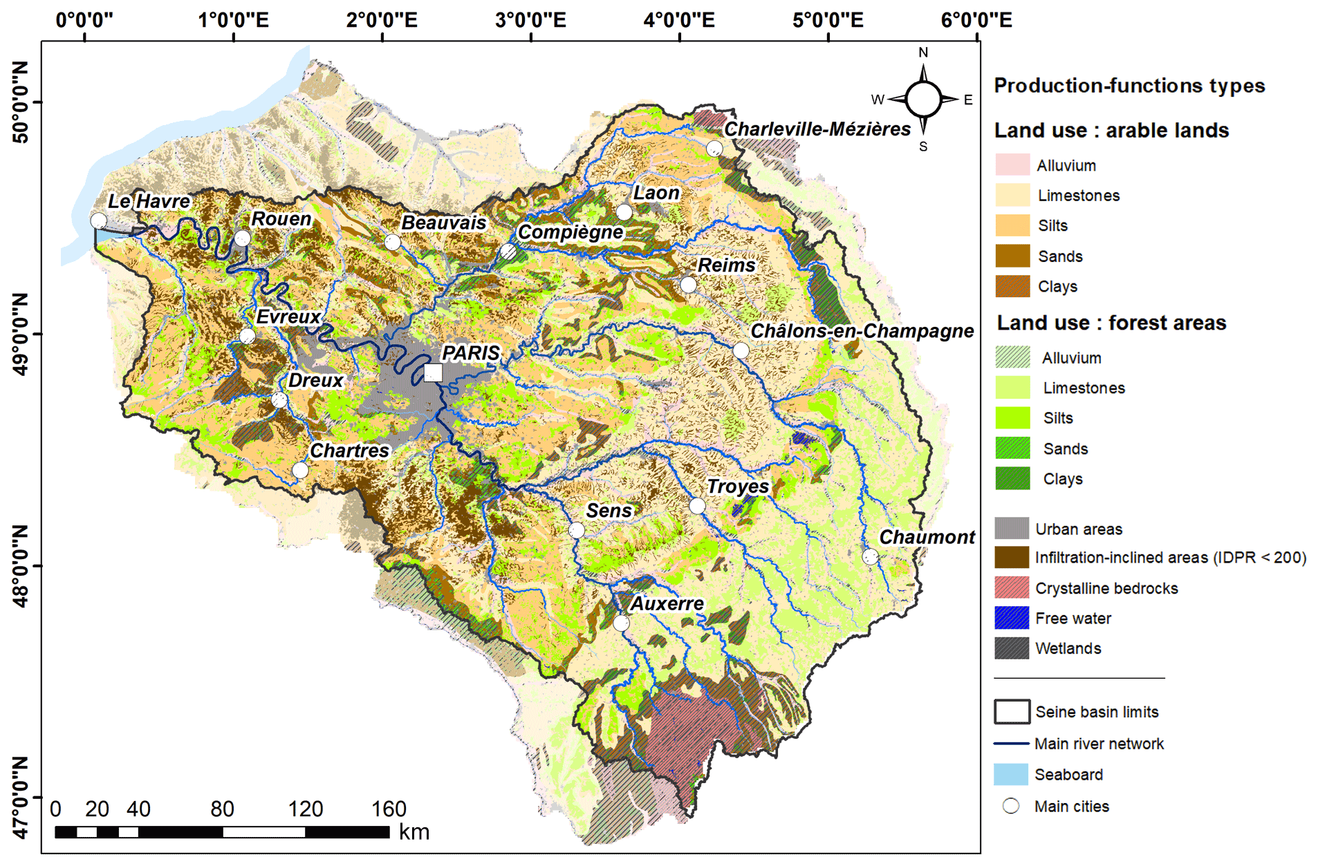
Figure 1Joint representation of land use and dominant lithology through production function distribution over the modeled area. Hatched zones highlight functions with a lower minority share in total surface (i.e., ≤2 %), which are excluded from the HYMIT–MCMC analysis.
We therefore develop a new fitting methodology based on a thorough analysis of hydrological signal transformation by various components of a hydrosystem in a nested approach, which considers the conditionality of parameter fields on their input forcing fluxes. The approach is based on the decomposition of hydrological signals in the Fourier frequency domain with the HYMIT method (Schuite et al., 2019).
2.1 The Seine River basin
2.1.1 A highly anthropized river basin
The Seine River basin (≃76 000 km2) is a highly human-impacted basin with a population of 17 million inhabitants. It receives the highest anthropogenic pressure in France due to the industry and agriculture linked to the development of the urban area of Paris, which coexists today with highly productive agricultural areas (66 % of the basin area, Fig. 1). For more information on the Seine basin, please refer to Billen et al. (2007) and Flipo et al. (2021b).
The river network is composed of 28 000 km of perennial rivers (Fig. 2). Overall, 97 % of the river network lies within the sedimentary Paris basin (Guillocheau et al., 2000), the largest GW reservoir in Europe. The interannual mean values (2003–2020 period) of the climate forcing (SAFRAN database – Quintana-Seguí et al., 2008) are 766 and 890 mm a−1 for precipitation and potential evapotranspiration (PET), respectively. The interannual module of the Seine river at Vernon (Fig. 2) is 477 m3 s−1 (2010–2019, http://hydro.eaufrance.fr/, last access: 4 January 2023, HYDRO database daily dataset).
Water withdrawals in surface water and GW amount to 3 km3 a−1. The pressure on water resources is high, especially during low-flow periods, when river discharges are sustained by GW and by human-built reservoirs (Fig. 2), totalling 841×106 m3.
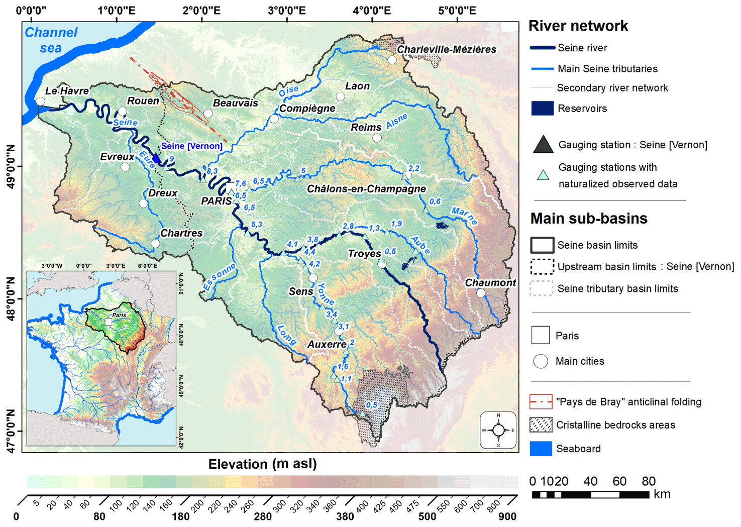
Figure 2General overview of the Seine basin area. A 25 m resolution DEM is used as the map background. Light blue labels refer to travel times (in days) from reservoirs to downstream discharge gauging stations (a.s.l.: above sea level).
2.1.2 Naturalization of downstream discharges from reservoirs
Here, observed river discharges are studied as an overall integrator of the system's behavior and response to climatic fluctuations. In this context, preliminary corrections are required to ensure the absence of anthropogenic disturbances in measured data that might result from the significant pressure the basin is submitted to. Since the HYMIT approach is not designed to dissociate such perturbations in measured discharge variations, the imprints left in the observed data by water reservoir storage–release cycles have been subtracted from downstream station records. Two types of information were used to perform this discharge naturalization: (i) reservoir withdrawn or released volumes to the river system and (ii) water travel times along the network respectively associated with each downstream station from one or several reservoirs.
The calculation of a naturalized discharge value [m3 s−1] associated with its respective actual measurement [m3 s−1] is performed using Eq. (1), written in the case of a station i at a time t located downstream from N reservoirs:
where [m3 s−1] represents the daily volume either stored from (>0) or released to (<0) the river system, accounting for the water travel time [s] along the network fraction between dam k and station i.
Travel times are calculated for each reach r of the network using a relative transfer time index as a function of geomorphological data (Golaz-Cavazzi, 1999; Flipo et al., 2012):
-
the distance dl(r) [m] between center of reach r and its contiguous downstream reach;
-
reach slope s(r) [–] derived from a digital elevation model (DEM);
-
the cumulative reach upstream drainage area S(r) [km2] and a calibration parameter γ=0.25 (Korkmaz, 2007).
For every reach, a relative transfer time index to the basin outlet is calculated as a sum of local Itr along all reaches leading to the outlet. A travel time is then calculated following Eq. (2):
where Itr;max is the maximum relative time index to the outlet basin and Tc [s] is the basin global concentration time, considered equal to 17 d (Gomez, 2002; Saleh et al., 2011; Pryet et al., 2015).
Naturalization of discharge records was carried out for the 30 measurement sites mentioned in Fig. 2, for which travel time values from reservoirs to stations (in days) are also displayed. In the case of several upstream reservoirs, labels correspond to mean travel time values.
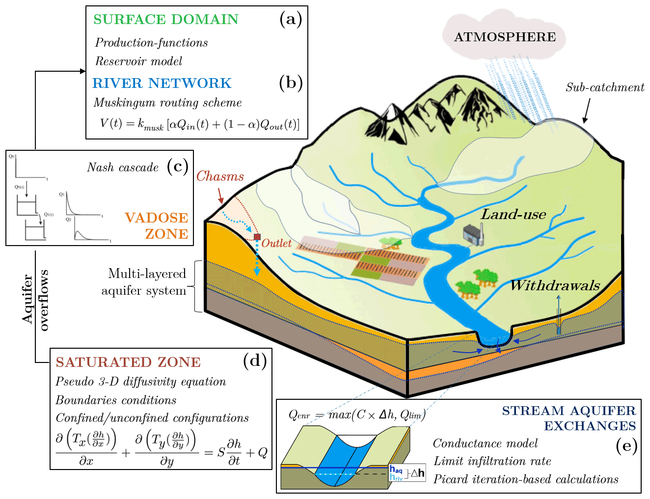
Figure 3Simplified illustration of the structure of the CaWaQS3.02 hydrosystem modeling platform and its main concepts involved in water flow calculations. Notations are as follows. (b) River network – α: a weighting parameter (∈ [0;1] ), kmusk: transfer time between two adjacent river elements, (Qin, Qout): river element input and output discharges, V: water volume contained in a river calculation element. (d) Saturated zone – (Tx, Ty): transmissivity coefficients in the x and y directions, S: storage coefficient, Q: source term. (e) Stream–aquifer exchanges – C: conductance coefficient, Qenr: stream–aquifer exchanges flow, Qlim: river-to-aquifer limit infiltration rate, Δ h: difference between water height in the river (hriv) and aquifer hydraulic head (haq).
2.2 The physically based coupled surface–subsurface model CaWaQS3.02
The physically based CaWaQS coupled model (CAtchment WAter Quality Simulator – Flipo et al., 2005, 2007b, a, 2021a; Labarthe, 2016) was used to (i) estimate the distributed effective rainfall over the basin as an input of a distributed HYMIT analysis at 221 river discharge gauging stations, (ii) estimate the basin physical parameters, and (iii) model the Seine basin pluri-decennial functioning. Based on the blueprint first published by de Marsily et al. (1978) and implemented as the MODCOU–NEWSAM software suite (Ledoux et al., 1984, 1989), CaWaQS3.02 (Flipo et al., 2022b) is a spatially distributed model that simulates coupled water, matter, and energy balances as well as flow dynamics within all compartments of a hydrosystem. The software structure links dedicated C-ANSI libraries meant to mimic main physical processes controlling the fate of water in each compartment. Calculations of surface, subsurface, and GW dynamics involve five main modules using a daily time step (Labarthe, 2016).
-
The first is a surface module (Fig. 3a), which computes estimates of actual evapotranspiration (AET), runoff, and infiltration fluxes (see Fig. A1 in Appendix A for more details). Relying on a conceptual reservoir-based approach (Girard et al., 1980; Deschesnes et al., 1985), water balance calculations account for climate data (see “total rainfall” and PET maps in Fig. 9a and b, respectively) as well as the distributions of land use and parent soil material (Fig. 1). Runoff water production is aggregated according to local subcatchments to ensure its direct transfer to the river system. These catchments can also be set up as runoff short circuits toward the unsaturated zone (“chasm”-type configuration). Details on the surface module are available in the Supplement with a special emphasis on AET calculation.
-
The second is a vadose zone module (Fig. 3c), which vertically transfers infiltration from the surface domain to subsurface outcropping aquifer areas. It diffuses soil infiltration based on a Nash reservoir cascade (Nash, 1959; Besbes and De Marsily, 1984) toward the aquifer system, which is equivalent to a gamma distribution function. This approach is an efficient and performing alternative to the Richards formulation of water flow in an unsaturated porous media below the root zone (Besbes and De Marsily, 1984). It is particularly well-adapted at the regional scale for analyzing groundwater level fluctuations (see for instance the recent studies of Cao et al., 2016; Jeong et al., 2018; Park et al., 2021) when preferential flow paths (Mirus and Nimmo, 2013; Nimmo, 2020a, b; Nimmo et al., 2021) are negligible, even though 10 % to 40 % of very deep aquifer recharge can originate from young water flowing through those preferential flow paths (Jackson et al., 2022).
-
The third is a groundwater or aquifer system module (Fig. 3d) based on the pseudo-3-D diffusivity equation (de Marsily, 1986), which is solved using a semi-implicit finite-volume numerical scheme, applied to nested grids. Besides integrating water recharge and anthropogenic withdrawals, it accounts for both confined- and unconfined-related resolution particularities and also handles, along time and space, reversible transitions between these two states. Exchanges between aquifer units are simulated based on a 1-D vertical simplification of water fluxes, which are assumed to be linearly connected to the head difference between aquifer units.
-
The fourth is a nonlinear conductance model (Fig. 3e), which accounts for a limitation of the infiltration flux in the case of disconnection (Brunner et al., 2009; Rivière et al., 2014; Newcomer et al., 2016), integrated within a Picard-iterative approach to compute stream–aquifer exchanges (Rushton, 2007; Ebel et al., 2009; Flipo et al., 2014).
-
The fifth is a hydraulic module (Fig. 3b), which transfers in-stream water discharges using a Muskingum routing scheme (David et al., 2011, 2013). For each river network cell, computed discharges integrate stream–aquifer fluxes, inputs due to subsurface runoff, and exogenous point injection flows.
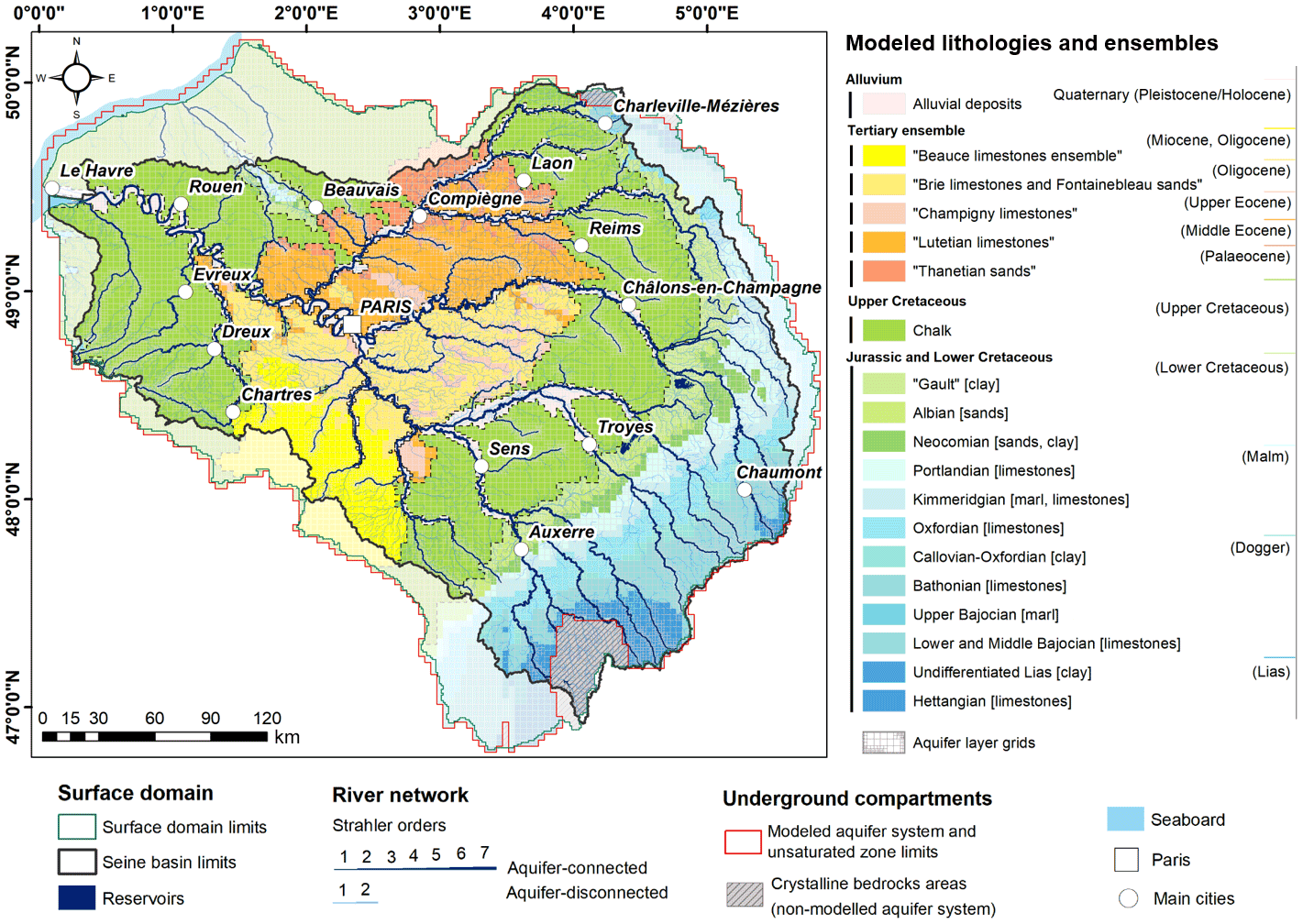
Figure 4CaWaQS–Seine application structure overview. Modeled lithologies are gathered according to the main ensemble they belong to. Ensemble limits are delineated on the map using dashed lines. Where appropriate, the most common formation names are used in quotation marks, and dominant lithology types are mentioned in square brackets.
Initially designed by Gomez et al. (2003) and later improved on by Pryet et al. (2015), Labarthe (2016), Baratelli et al. (2018), and Flipo et al. (2021a), the Seine basin application accounts for the following:
-
a surface layer (≃95 100 km2), divided into elementary calculation cells of 11 km2 in average size, which covers the entire Seine basin;
-
a river network that corresponds to 6830 km of rivers (mainly due to computational time concerns, calculations of stream–aquifer exchanges have been constrained to rivers including reaches with Strahler orders from 3 to 7 or 8 depending on the definition of perennial rivers in the database used to define the river network; Strahler, 1957);
-
and a multi-layered aquifer system divided into 20 lithology units. These units are meshed using multi-scale nested grids with square-shaped cells ranging from 3200 to 100 m in size. From the oldest to the most recent, these units can be regrouped into four main categories (Fig. 4): (i) an alternating ensemble of aquifer and aquitard units, mostly made of limestone and marl–clay associations, respectively – as a whole, they range from Lower Jurassic (Hettangian stage, −195 Myr) to Lower Cretaceous (Albian stage, −100 Myr) and mostly outcrop on the eastern end of the basin; (ii) a large Upper Cretaceous chalk layer; (iii) a five-layer Tertiary complex ensemble located in the center of the basin, which covers units mainly made of limestone and sand, dating back from the Paleocene to Miocene stages; and (iv) recent alluvial deposits (Pleistocene and Holocene stages from −2.5 Myr to −10 000 years, respectively) surrounding the main rivers. Areas where crystalline bedrock outcrops (Morvan, Ardennes) are not explicitly simulated (≃1.9 % of total modeled surface) (Fig. 2).
2.3 Minimalist reduction of frequency domain hydrological data with HYMIT
The HYMIT (HYdrological MInimalist Transfer function) method was designed by Schuite et al. (2019) and Schuite (2022) to describe how hydrosystems transform a climatic input signal, namely effective rainfall, into observed hydrological responses such as river discharges or GW levels. Based on previous theoretical developments in the field of stochastic hydrology and frequency domain analysis of hydrological variables (Gelhar, 1974; Molénat et al., 1999; Russian et al., 2013), HYMIT features a complete yet simple characterization of the filtering effects on flow dynamics by the three main compartments in a hydrosystem: the surface (runoff, taking into account overland and hypodermic flow), the unsaturated porous subsurface (vadose zone), and the saturated subsurface (aquifer system). In other words, it links the expression of multi-frequency climate variability in GW levels and river discharges to the hydraulic and hydrogeological properties of hydrosystems through a transfer function analysis in the frequency domain. In practice, HYMIT is adjusted to experimental transfer functions built from the discrete Fourier transforms of effective rainfall and river discharge time series. Therewith, it is possible to rapidly obtain a first-hand estimation of key watershed properties by taking advantage of the full statistical power of long time series and the tractable analytical description of a catchment's hydrological functioning (Pedretti et al., 2016; Jiménez-Martínez et al., 2013; Jimenez-Martinez et al., 2016; Manga, 1999; Molénat et al., 1999; Schuite et al., 2019).
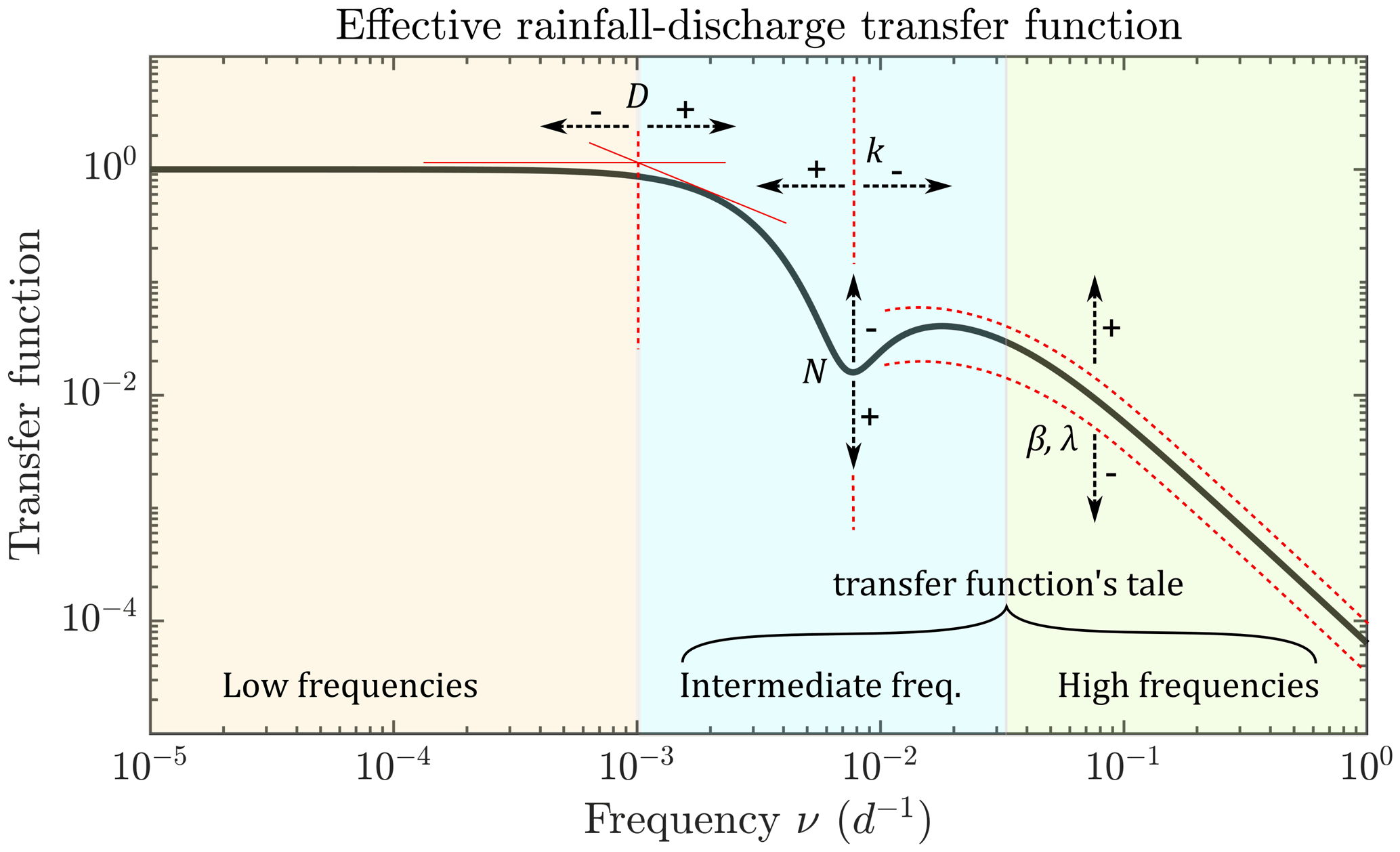
Figure 5Example of effective rainfall to river discharge transfer function as modeled by HYMIT (Schuite et al., 2019), with a representation of the main influence of each parameter on its shape. The parameters are D the hydraulic diffusivity of the aquifer compartment, N the number of reservoirs in the Nash cascade representing the flow transfer through the unsaturated zone, k their emptying constant, β the fraction of effective rainfall flowing through a watershed as surface runoff, and λ the decay coefficient associated with it. Arrows accompanying a positive sign + (negative sign −) show the TF's direction of change as a result of an increase (decrease) in the parameter's value. Note that the shape of HYMIT is highly variable and is ultimately the result of a complex interplay between all parameters, which cannot be fully captured in this general depiction.
The ratio of the power spectral density (PSD) of the naturalized river discharge over that of effective rainfall gives an experimental transfer function (ETF) (Pedretti et al., 2016; Schuite et al., 2019). The PSD of a signal is obtained by squaring the module of its Fourier transform, which is computed using a classical fast Fourier transform algorithm (“fft” function in MATLAB). An MCMC inversion procedure is implemented to adjust HYMIT to each ETF in order to estimate all controlling parameters for all sub-basins for which discharge data are available. The MATLAB package of Haario et al. (2006) for MCMC inversion is used with the built-in Metropolis–Hastings sampler. In the case of effective rainfall discharge analysis with HYMIT, five parameters control the shape of the transfer function (TF) and thereby the climatic signal's transformation representation (Schuite et al., 2019) (Fig. 5):
-
the hydraulic diffusivity of the aquifer compartment D [m2 s−1] – this parameter controls the position of the first slope rupture in the TF, where it departs from a horizontal asymptotic line of equation y=1 (the rupture slides to higher frequencies for increasing values of D);
-
the number of cascading linear reservoirs representing the transfer in the unsaturated layer N [–];
-
the emptying constant of these reservoirs k [d] – these two last parameters control the amplitude and partly the horizontal position of the local depression sometimes observed in the TF at intermediate frequencies (high values of k×N tend to exacerbate the prominence of this central energy loss);
-
the fraction of effective precipitation transiting to the outlet through the surface compartment β [–] – this parameter partly controls the shape of the transfer function at intermediate frequencies and high frequencies (indeed, increasing β gives more energy – in terms of spectral density – to fast surface flow processes, thereby driving parts of the transfer function's tale upwards);
-
and the characteristic runoff timescale λ [d−1]. Together with β, this parameter modulates the shape and position of the TF's tale and may also affect the amplitude of the depression created by the transfer through the vadose zone.
Schuite et al. (2019) demonstrated that HYMIT is sensitive to all parameters on both a synthetic case study and real data, but the shape of the TF is ultimately governed by a complex interplay between physical properties of hydrosystems and the characteristic flow timescales they induce in each hydrologic compartment. For instance, the central energy depression in the TF, known to appear in the presence of a strongly inertial unsaturated zone, was observed for the Essonne watershed but not for the Aube watershed, yet both are nested within the Seine basin (Schuite et al., 2019).
The method requires knowledge of the effective rainfall, which is not directly measured. It therefore needs to be assessed by a surface balance model. In this study, the surface module of the hydrological model CaWaQS3.02 is used (see Sect. 2.2) for both practical reasons (spatialized soil, land surface data availability, and integration) and consistency concerns with subsequent fitting steps. The fitting of the surface balance model is detailed in the Sect. 2.4.
A total of 384 discharge gauging stations are (or were) operational across the different rivers of the Seine basin. Daily discharge data were checked for completeness and overall quality. In the presence of any gap longer than 10 % of the total series length, the station was discarded from the analysis. So were stations with overly short records (less than 10 years) to maximize the statistical power of the analysis. Small gaps are filled by linear interpolation. Minor data errors were corrected, such as inconsistent timelines, double records, or negative values. After data curation and selection, discharge series from 221 stations remained. Prior to Fourier transformation, all time series are detrended and windowed using a Hanning tapering function.

Figure 6Illustrated flowchart of the full stepwise HYMIT–CaWaQS fitting procedure. Notations with overbars indicate integrated variables over time. Variable space and/or time dependencies are mentioned using -type notations. AET: actual evapotranspiration, β: effective precipitation fraction transiting to the catchment outlet through the surface compartment, h: hydraulic head, k: emptying constant of Nash cascade linear reservoir, λ: characteristic runoff timescale, P: rainfall, Pe: effective rainfall, PET: potential evapotranspiration, Qenr: stream–aquifer exchange flow, Qi: infiltration flow, Qnat: naturalized observed river discharge, Qout: discharge at sub-basin outlet, Qr: runoff flow, T: transmissivity coefficient, and S: storage coefficient.
2.4 Stepwise fitting methodology based on a nested hydrological approach
A nested fitting method is proposed (Fig. 6). It is based on the identification of the CaWaQS3.02 model parameters, process by process, on the basis of measurable quantities. It is considered nested due to the conditionality of the parameter fields on their forcings. Each step is developed with this conditionality idea in mind. Roughly, the first step considers the estimation of the partitioning of the rainfall into AET and effective rainfall, while the next one focuses on the partitioning of effective rainfall into fast runoff and slow infiltration. The last steps deal with regulating the velocities of both surface and subsurface flows.
The first step of the fitting methodology consists of estimating the total AET at the basin scale from the average discharge of water flowing out of the basin (Fig. 6, step 1). In order for this average to exist mathematically, it is then necessary to reproduce the flows averaged over 17 years, which is the stationarity period of this signal (Flipo et al., 2012; Massei et al., 2010, 2017). In the surface balance module, the set of parameters regulating actual evapotranspiration (AET) flow simulation is adjusted using an MCMC approach aimed at minimizing the discrepancy between the long-term average discharge at the watershed outlets and the long-term average meteoritic net input over the watershed impluvium (i.e., the effective rainfall that corresponds to water available for flow within the basin). Furthermore, we selected a total of 35 reference sub-basins across the Seine hydrosystem satisfying two criteria, namely good spatial coverage of the basin as well as long and complete daily discharge time series.
Before proceeding with the fitting of the model parameters themselves, sets of distributed minimalist hydrological parameters are estimated at 221 gauging stations in the basin using the HYMIT method (Fig. 6, step 2). The following steps of the fitting procedure are based on these estimates with the objective each time to spatially reproduce the variability of these minimalist parameters with the process-based model used, e.g., CaWaQS. In other words, the wealth of information provided by the quantified and regionalized estimates of HYMIT parameters is used as the only support for the fitting of the surface and subsurface water flow calculation within the model. Thus, this step enables the transition from a point assessment to a continuous spatiotemporal characterization of the regional hydrosystem behavior.
The third step consists of adjusting a parameter of the water production cells in order to reproduce as closely as possible the effective rainfall partitioning evaluated by HYMIT (β coefficient, Fig. 6, step 3).
The fourth step deals with the temporal synchronization of fast runoff estimated by the process-based model using the estimate of this quantity obtained with HYMIT at each discharge gauging station (λ coefficient, Fig. 6, step 4). The attribution of λ coefficient values identified with HYMIT to the corresponding CaWaQS parameter is made by analogy. For each gauging station, a spatial analysis is performed to calculate the proportion of the CaWaQS hydrological units that comprise the catchment of the station. Over the Seine basin, it is possible to identify a sufficient number of upstream catchments that are mostly composed of a single CaWaQS hydrological unit. For each of these catchments, the CaWaQS parameter is set up in a straightforward way, simply equating it with the value of the HYMIT λ coefficient.
Until now, all the steps were focused on surface processes. The proper simulation of these processes is crucial since they allow us, among other processes, to estimate a distributed recharge toward the aquifer system. The fifth and last step of the methodology is carried out differently for the vadose zone than for the aquifer system and is divided into three substeps.
-
The first is a preliminary coarse calibration of transmissivity parameter fields for each model aquifer layer, performed in steady state. A trial-and-error approach is used to adjust simulated water tables to mean level values measured at control wells. To achieve this step, an aquifer compartment-only simulation is implemented. A mean aquifer recharge field, calculated over two 17-year cycles (i.e., 1986–2020 period), derived from the HYMIT-calibrated CaWaQS surface module, is used to constrain the simulation ( in Fig. 6, step 5).
-
The second is a fitting of the Nash cascade parameters, namely k and N (see Sect. 2.3 and 2.2). Usually associated with lithology, HYMIT-k values are spatially distributed along a functional sectorization combining two information types: dominant soil textures (Fig. 1) and upmost free aquifer formation lithology (Fig. 3). For each association identified, attribution of k values is made using an analogy method, as previously described in the case of HYMIT λ coefficient distributions (see Sect. 2.4). N parameter field, reflecting unsaturated zone thickness, is geometrically defined based on the difference between subsurface adjusted water levels in steady state and ground elevation, while considering a single reservoir to be representative of an elementary 5 m thickness. Overall, at the basin scale, k parameter values range from 2 to 9 d. Tertiary terrains are mostly associated with low thickness values from 0 to 20 m, while they range up to 40 m within the chalk impluvium limits (Fig. 12). An unsaturated thickness map (not shown) noticeably depicts high values up to 135 m in the southern part of the east border of the basin.
-
The third involves finer manual adjustments of parameter fields regulating both water levels and dynamics, namely transmissivity (T), storage (S), and conductance (C) coefficients. To do so, iterative transient-state coupled model runs are performed, constrained by daily time step HYMIT-calibrated infiltration fluxes (Qi(t) in Fig. 6, step 5). T and S parameter distributions are manually tuned based on expert knowledge of regional aquifer functioning and also accounting for piezometric reference maps as well as pumping test values, where available. In order to minimize the number of parameters to be adjusted, conductance fields, which regulate surface–subsurface interactions (i.e., stream–aquifer exchanges and overflows from the aquifer to the surface), are automatically calculated and updated to be consistent with successive T fields following the methodology proposed by Rushton (2007). They have been implemented in a previous version of the Seine model by Pryet et al. (2015) and also successfully used on the Loire basin by Baratelli et al. (2016). The performance of each trial is assessed at the scale of each control point, combining statistical criteria calculations and visual comparisons between simulated and observed time series (see Sect. 3.2 and 3.3). This initiates a trial-and-error fitting process, alternating between hydrodynamic parameter modifications and run quality evaluation, until satisfactory performance is reached.
Prior to any subsurface fitting work, GW withdrawals are integrated into the application in order to account for anthropogenic-induced disturbances to the aquifer system. Data consist of spatially located annual volume time series. Depending on the type of water usage, annual values were either linearly distributed over the year (drinking water, industry) or specifically dispatched over the summer season (irrigation).
The next two sections exemplify the power of the stepwise methodology applied to the regional scale of the Seine basin.
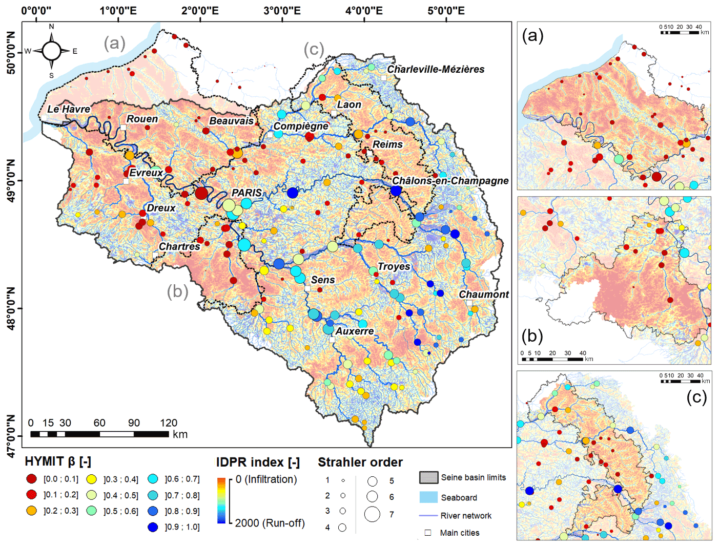
Figure 7Spatial comparison between HYMIT β and IDPR values at the Seine basin scale. Local focuses: (a) Pays de Bray–Pays de Caux, (b) Beauce, and (c) Craie Champenoise.
As mentioned in Sect. 2, the stepwise fitting methodology relies on a distributed assessment of physical parameters that control the partitioning of hydrological fluxes within watersheds. Before reviewing the performance of the coupled CaWaQS–Seine model, we therefore qualitatively review the results of the distributed HYMIT analysis at the Seine basin scale. Section 3.3 and 3.2 propose a more classic assessment of the model performance, comparing simulated values with measurements of river discharges and GW hydraulic heads.
3.1 Qualitative analysis of spatially distributed infiltration fluxes estimated with HYMIT
The average partitioning of effective rainfall between surface runoff and deep infiltration is adjusted based on the HYMIT β parameter. This parameter is generally poorly constrained at large scale, especially its spatial distribution. Hence, very little information is available to compare our β estimates against and, ultimately, to validate them.
Fortunately, the French Geological Survey (BGRM) has developed a systematic method to qualify the propensity of terrains to either infiltrate water or to generate runoff, as described by Mardhel et al. (2021). The method takes advantage of the mismatch evaluated between thalweg locations inferred from digital elevation models and the actual location of drainage networks used to build a normalized index called IDPR (Network Development and Persistence Index). The lower its value, the more a terrain is prone to infiltration and vice versa. Mardhel et al. (2021) calculated this index for the entire French metropolitan area at high resolution (25 m). We take this opportunity to qualitatively assess the consistency of β estimates, which, in a way, is very complementary to the IDPR, being much less spatially resolved but providing an actual operable value to the flow partitioning, which is of primary importance for modeling purposes.
Table 1Distribution of coupled model performance criteria (2003–2020 period) on GW simulation. Upper table (range values in meters): root mean square error (RMSE), mean absolute error (MAE). Lower table (nondimensional range values): Pearson correlation coefficient (Cpearson) and Kling–Gupta efficiency coefficient (KGE).
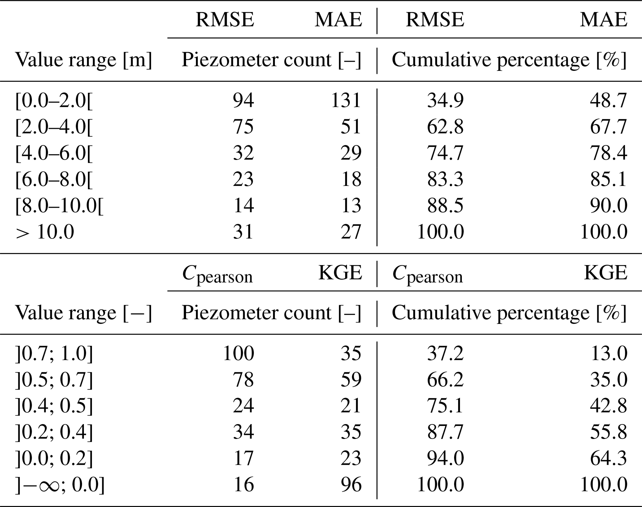
Table 2Distribution of coupled model performance criteria (2003–2020 period) on river discharge simulation. Nondimensional range values. Nash–Sutcliffe efficiency (NSE) and Kling–Gupta efficiency coefficients (KGE).
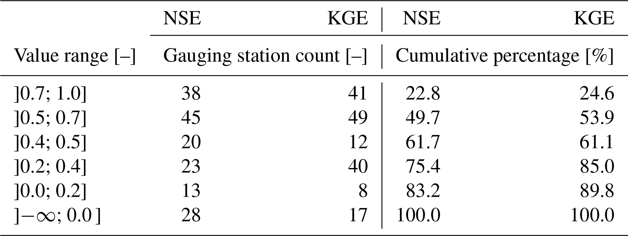
Figure 7 superimposes estimates of β at each discharge gauging station (dots) and the IDPR map produced by Mardhel et al. (2021). First, an overall spatial coherence is observed between these two indicators. Upstream stations experience medium to high runoff components (β>0.2), especially in the eastern and southern fringes of the basin. These regions entail a dominant proportion of medium to high IDPR areas as well. Conversely, areas dominated by low IDPR values are drained by rivers where low values of β are found. We further note a satisfactory sectorial coherence in β estimates: two low-order rivers draining the same geomorphological units exhibit close properties in terms of flow partitioning. This aspect is particularly well-established in the Beauce and Craie Champenoise regions (Fig. 7b and c, respectively). It is also the case for the southern regions of the Morvan (see Fig. 2); yet in this case β values seem comparatively low with regard to the high IDPR values, possibly underscoring a more complex interplay between different runoff-generating mechanisms in this sector (slope, soil structure, geology, etc.).
Another marker of consistency is present in the northwestern part of the basin in and around the Pays de Bray sector (Fig. 7a). The Pays de Bray anticline is characterized by the local emergence of sandy and clayey Jurassic terrains with high slopes, extending NW–SE (see Fig. 2), among Upper Cretaceous carbonate subplanar units (see Fig. 4). Therefore, property contrasts between these terrains are clearly distinguishable in IDPR values and are also well-captured by the flow partitioning estimation with the HYMIT, as the river draining the Pays de Bray anticline displays a β value of approximately 45 % to be compared with the very low values found on adjacent stream networks (β<10 %).
3.2 Simulation of hydraulic heads in aquifers
Within the modeled aquifer system limits, 340 head observation time series are compiled from the national ADES database (https://ades.eaufrance.fr/, last access: 4 January 2023). Raw data curation is performed based on the minimum covered time span and a threshold number of observation data. Time series on which GW dynamics are not clearly identifiable are discarded as are measurement sites located in local non-modeled formations (e.g., perched water tables). In all, 269 GW control points with data suited for aquifer calibration are selected.
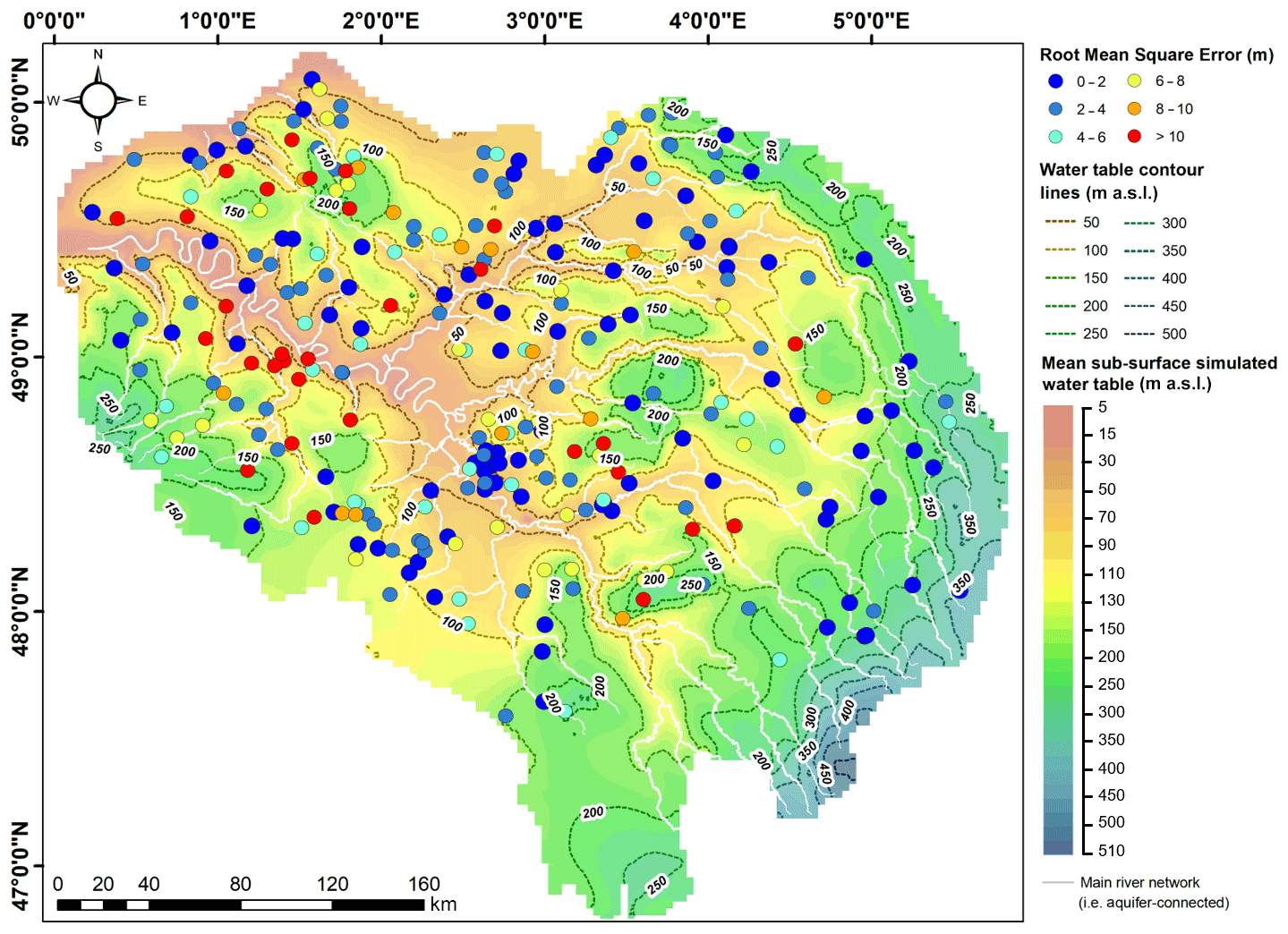
Figure 8RMSE criteria for GW simulation over the 2003–2020 period (see also Table 1). The water table contour lines (50 m span) and background map depict the spatial evolution of simulated mean GW levels for all uppermost aquifers (subsurface) over the same period (a.s.l.: above sea level).
Calculated over the 2003–2020 calibration period, RMSE (root mean square error), MAE (mean absolute bias), Pearson correlation coefficient, and KGE (Kling–Gupta efficiency) (Gupta et al., 2009; Kling et al., 2012) are used to assess model performance (Table 1). GW simulation exhibits satisfactory performance overall as nearly two-thirds of control points are associated with both RMSE and MAE values below 4 m (63 % and 68 %, respectively). A total of 66 % of piezometers show correlation coefficients above 0.5, demonstrating the model ability to mimic the great multiplicity of aquifer dynamics encountered at the regional scale. Less clear-cut performance results (43 % of points) are obtained regarding a proper joint reproduction of the evolution of both levels and dynamics (KGE >0.5). General aquifer RMSEs and MAEs are 5.4 and 4.7 m, respectively. At the model layer scale, mean RMSE and MAE fit in the 0.9–6.7 and 0.4–6.5 m ranges, respectively. Unsurprisingly, lower values are calculated for alluvial formations (1.4, 1.2 m) and the Jurassic ensemble (1.5, 0.6 m), as most control points are constrained by proximal river drainage levels. RMSE score maps (Fig. 8) show a homogeneous distribution of lower values over the entire basin, apart from the Evreux–Dreux area (left bank of the downstream Seine River, see Fig. 2) gathering the highest misfits, where local disturbances of aquifer flows are known to be heavily karst-induced (El Janyani et al., 2012), making them harder to reproduce by the model.
3.3 Simulation of river discharges
Similarly to raw piezometry data, pre-processing work is carried out on river discharge observations using data compiled from the HYDRO database (http://hydro.eaufrance.fr/, last access: 4 January 2023), totalling 384 river stations (see Sect. 2.3). As previously stated, since calculations of stream–aquifer exchanges are constrained to the main river network (see Sect. 2.2 and Fig. 4), only 167 discharge gauging stations are considered as valid discharge calibration control points. Usual Nash–Sutcliffe (Nash and Sutcliffe, 1970) and Kling–Gupta efficiency coefficients (labeled NSE and KGE, respectively, in Table 2) are selected to evaluate simulation performances on river discharges.

Figure 9Mean distribution fields of (a) “total rainfall” (i.e., the sum of liquid rainfall and snowfall, which is almost nil at the Seine basin scale), (b) PET, (c) AET, and (d) effective rainfall over the 2003–2020 period (in mm a−1).
At the basin scale, 50 % and 53 % of control stations respectively show NSE and KGE scores above or equal to 0.5. The spatial distributions of both criteria (not shown) demonstrate that most of the higher values are noticeably distributed along the Seine River and its eight main tributaries (see bold blue lines in Fig. 2). For the 64 stations located along this network portion (2910 km, 43 % of total modeled network), 54 (26) of them are associated with KGE ≥0.5 (0.7). Noticeably, 44 stations combine both NSE and KGE values ≥0.5.
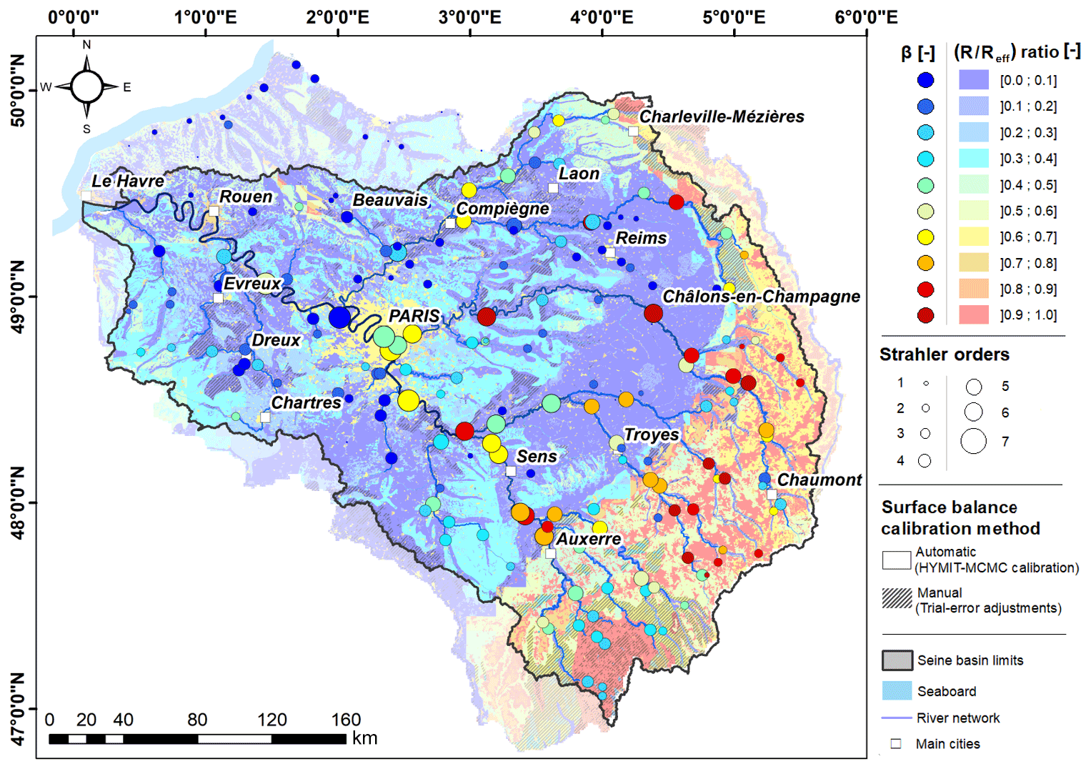
Figure 10Distributed partitioning of the pluri-annual mean effective rainfall calculated over the 1970–2018 period and expressed as a ratio between simulated runoff fraction (R) and total effective rainfall (Reff). HYMIT β values determined at discharge gauging stations are also indicated using point symbols.
Once the CaWaQS–Seine model exhibits satisfactory performances (see Sect. 3), it is used to estimate spatiotemporally distributed key hydrological fluxes such as effective rainfall (see Sect. 4.1), infiltration rates (see Sect. 4.2), surface runoff, and exchanges between aquifer units or between aquifers and rivers (see Sect. 4.3). Finally, all these data are synthesized by the Seine basin water balance, including water fluxes between aquifer units (see Sect. 4.4).
4.1 Distribution of effective rainfall
CaWaQS–Seine is first used to estimate the distribution of two important hydrological quantities over a period of 17 years (2003–2020): AET and effective rainfall (Fig. 9c and d, respectively), with the latter considered to be stationary during this period (see Sect. 2.4). They are both estimated from rainfall and PET (Fig. 9a and b).
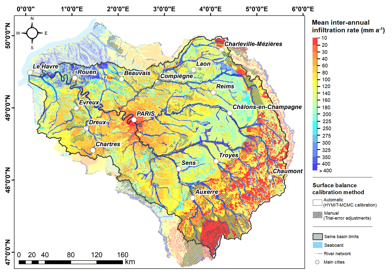
Figure 11Mean annual infiltration rates (in mm a−1) simulated by CaWaQS–Seine. Mean values over the 1971–2019 period.
The effective rainfall is highly contrasted across the Seine basin, ranging from 44 mm a−1 up to 918 mm a−1 locally (Fig. 9d). The lowest effective rainfall rates occur around the city of Paris and in the Eure basin, around Chartres and Dreux (see Fig. 2). The central part of the basin experiences an effective rainfall mainly lower than 130 mm a−1, while the eastern ridge, or Jurassic edge, experiences effective rainfall rates higher than 250 mm a−1, sometimes reaching 920 mm a−1 as is the case in the southern part of the basin in the Morvan area. It is also the case in Normandy in the northern part of the basin, called Pays de Caux (see Fig. 7a), in the north of Rouen.
4.2 Distribution of infiltration rates
A key piece of information for hydrogeologists and groundwater managers is the estimation of aquifer recharge. A complete water balance calculation using the CaWaQS model enables the simulation of effective rainfall, runoff, and infiltrated water distributions at the daily time step with a high spatial resolution. It is therefore possible to represent the average distributed partitioning of effective rainfall at the basin scale (Fig. 10) over the period 1970–2018, expressed as the ratio between the simulated runoff and the total effective rainfall.
Before further analyzing the estimated infiltration rates, it is important to note that the distributed effective rainfall partitioning estimated by CaWaQS–Seine is consistent with that obtained using the HYMIT analysis alone (Fig. 10), which is in agreement with the most advanced GIS-based analysis (Sect. 3.1). Indeed, the simulated predominance of the runoff process over the entire Jurassic edge of the basin (simulated local partitioning generally higher than 0.6) is in agreement with high β values in this area. The opposite observation can be made for the interior of the basin with low simulated partitioning values that agree with HYMIT low partitioning values for headwater streams in the area (lower than 0.3, Fig. 10).
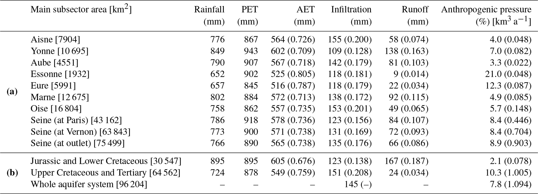
Distributed infiltration rates are then calculated as an interannual average over the simulation period 1970–2018 (Fig. 11). They balance the effective rainfall, mostly leading to relatively moderate infiltration rates (lower than 120 mm a−1) over the basin, except (i) on the Norman Pays de Caux north of Rouen where it can reach 400 mm a−1 and (ii) to a lesser extent over the chalk area. In particular, infiltration rates are controlled by the geology as it is lower in areas with high effective rainfall than in areas with lower effective rainfall: 123 mm a−1 over the Jurassic and Lower Cretaceous aquifer units and 151 mm a−1 over Upper Cretaceous and Tertiary aquifer units (Table 3).
There is also a spatial coherence between β and the infiltration rate from the point of view of land use, insofar as the predominantly agricultural (urban) areas are indeed marked by higher (lower) infiltration (see, for instance, the chalk area or the central Île-de-France that surrounds Paris). Also, the areas initially associated with very low IDPR values (fast infiltrating areas – see Fig. 1) clearly appear on the infiltration map, with infiltration rates higher than the regional average (see, for instance, the Pays de Caux area or the eastern of Chartres).
Finally, geological characteristics also emerge from the zoning, insofar as the sectors dominated by soils classically more permeable and conductive to infiltration (e.g., sands, alluvium) delimit areas of higher infiltration rates than the regional trend. Such a configuration is noticeable for regions such as the Sologne and Fontainebleau forest areas (see Fig. 1) or Thanetian sands and alluvium deposits (see Fig. 4).
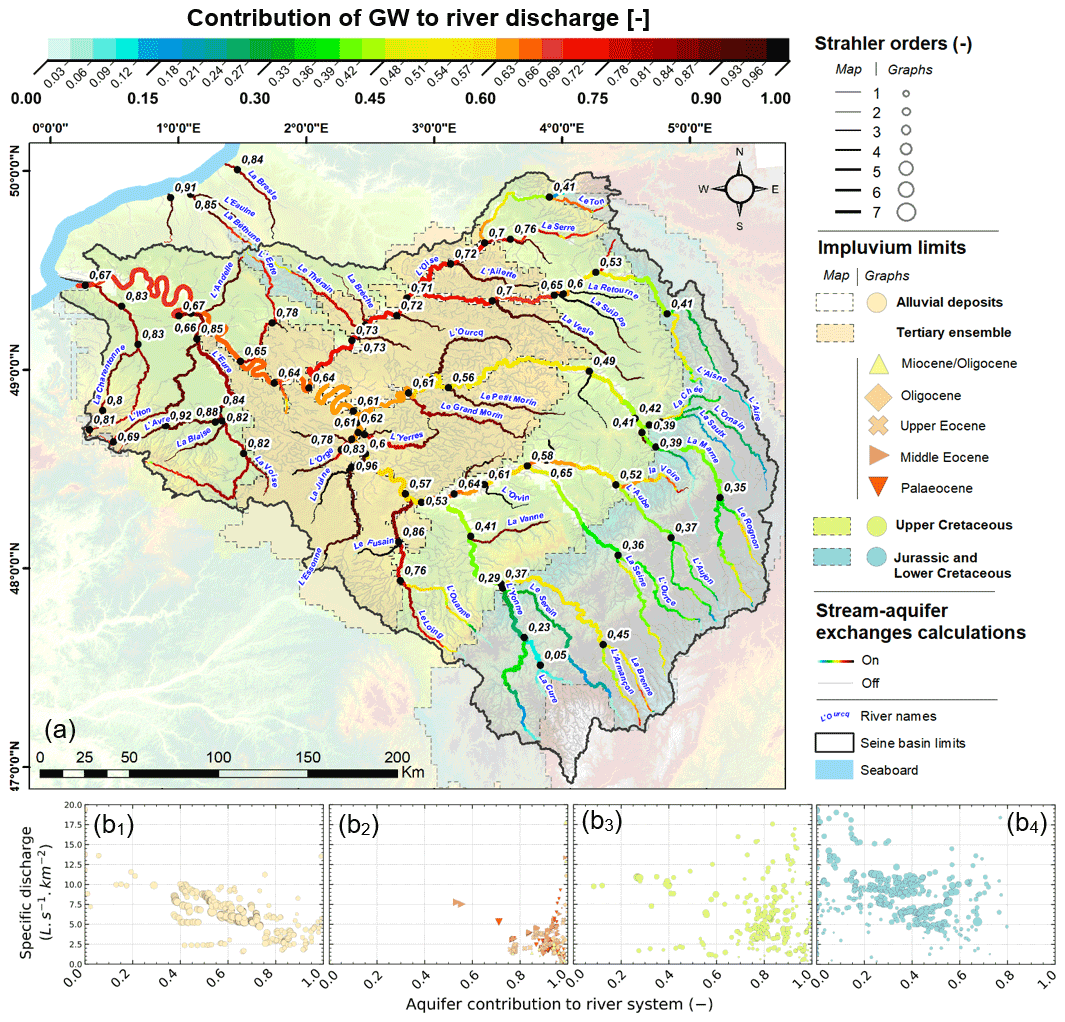
Figure 12(a) Distribution, at the river reach scale, of the aquifer system contribution to the river network. For each reach, values are expressed as a fraction (∈ [0;1]) of the network total input volume, calculated within the limits of its respective upstream watershed. Mean annual values are calculated over the 2003–2020 period. For the sake of readability, labels indicate the fraction value right after each confluence and outlet of the main network. (b) Relations between specific discharges in river (in L s−1 km−2) and aquifer system contribution (–) to the hydraulic network. Each point corresponds to a river reach. Panels gather data according to the layers the network is connected to. From the most recent (far left) to the oldest (far right): (b1) alluvial deposits, (b2) Tertiary ensemble, (b3) Upper Cretaceous–regional chalk aquifer, and (b4) Jurassic and Lower Cretaceous ensemble.
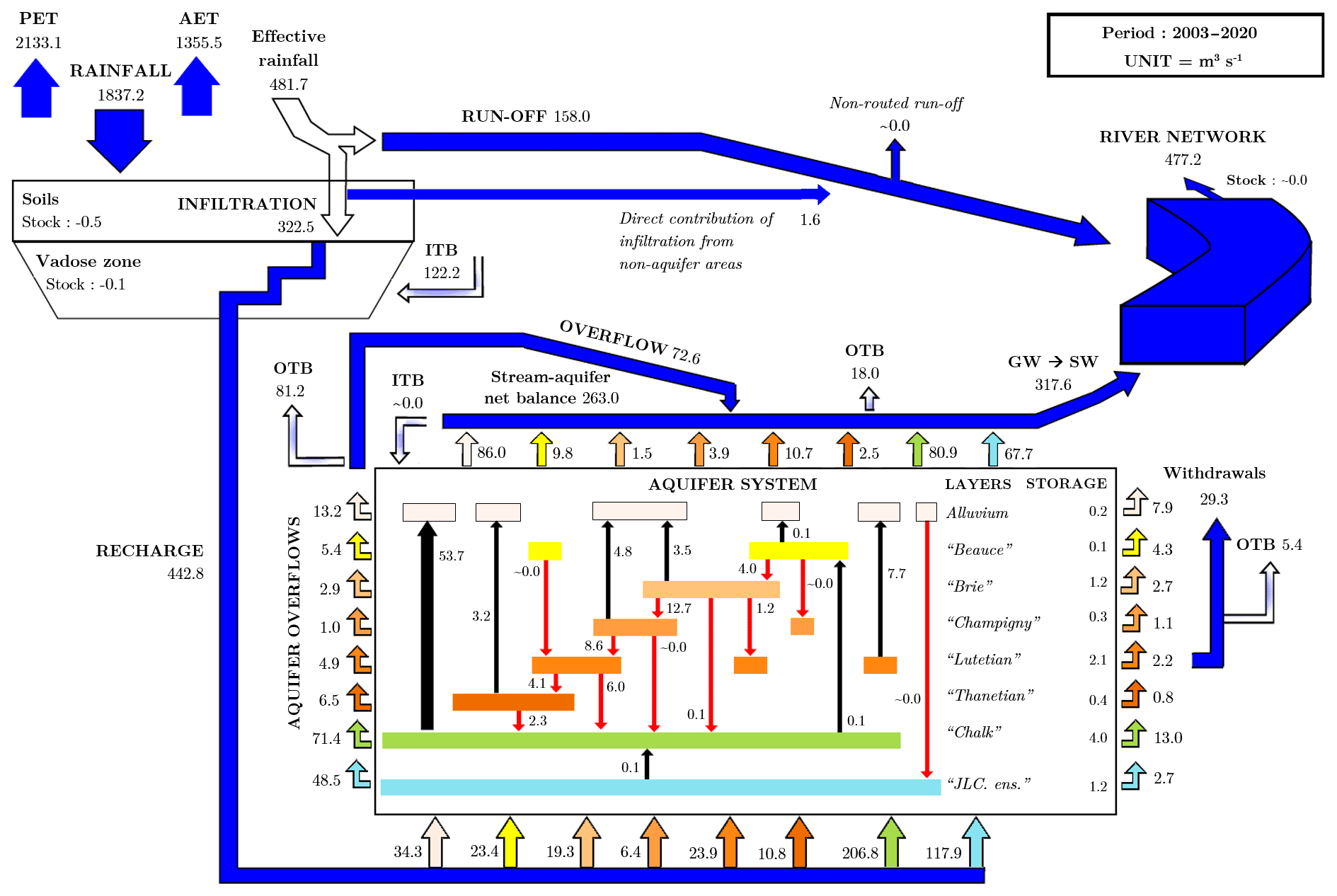
Figure 13Summary diagram of the structure and average functioning of the Seine hydrosystem, as simulated by the CaWaQS–Seine application. All flows are expressed as interannual average values (m3 s−1) over the 2003–2020 period. Beauce: Beauce limestones ensemble, Brie: Brie limestones and Fontainebleau sands, Champigny: Champigny limestones, Lutetian: Lutetian limestones, Thanetian: Thanetian sands, JLC. ens.: Jurassic and Lower Cretaceous. ITB: infiltration flux for outcropping aquifer units beyond the Seine basin limits (see Figs. 10 and 11). OTB: GW fluxes outflowing beyond the basin limits with vertical projection on GW system extension. The area of the Seine river basin is 75 499 km2.
4.3 Distribution of groundwater contribution to river discharges
Labarthe et al. (2015) and Pryet et al. (2015) were the first to publish a spatially distributed evaluation of stream–aquifer exchanges at the regional scale, exemplified with the Seine basin. At the time, they followed the stepwise fitting methodology of Flipo et al. (2012). Given the advances proposed in the current paper, we re-assessed those estimates (Fig. 12) based on the HYMIT functional analysis of the hydrological behavior of many sub-basins and also on the extension of the subsurface domain that is taken into account by the model.
The pluri-annual average (2003–2020) contribution of groundwater (GW) to river discharge is calculated along the river network of the Seine basin. Two specific patterns of spatial GW contribution to river baseflow appear in the Seine basin:
-
a longitudinal increase in the contribution of GW to river baseflow from upstream to downstream for river systems originating in the Jurassic edge of the basin;
-
and a very high contribution of GW to river baseflow over the tertiary (>0.75), alluvial (>0.4), or Upper Cretaceous (mostly >0.6) aquifer units (Fig. 12b).
Those patterns are confirmed by a spatial analysis of the statistical distribution of GW contribution to river baseflow regarding the specific discharge. Each analysis is made for each outcropping aquifer unit. For the Jurassic and Lower Cretaceous aquifer units, the lower the specific discharge, the higher the GW contribution to river baseflow, with the highest limit at 0.7 for a few small streams in the area (Fig. 12b4). For the small streams fed by GW from the Tertiary aquifer units, the GW contribution is always higher than 0.8 (Fig. 12b2). The GW contribution of the Upper Cretaceous aquifer unit is similar to that of the Tertiary aquifer units (Fig. 12b3), even though the absolute value of the contribution can be slightly lower in this area (0.5). As for the Jurassic and Lower Cretaceous edge of the basin, the GW contribution of alluvial GW to river discharge exhibits a decreasing GW contribution with the increase in the specific discharge that is correlated with higher Strahler orders (Fig. 12b1). But the GW contribution in alluvial aquifers is always higher than 0.4, which is a significant difference from the Jurassic edge.
4.4 Water budget
Finally, a water budget of the Seine basin is established (Fig. 13) over a 17-year cycle that ensures zero storage variations (Flipo et al., 2012).
A very large fraction (73.8 %) of rainfall is converted to AET (average value of 565 mm a−1). The remaining effective rainfall fraction, i.e., 26.2 % (average value of 201 mm a−1), is divided into infiltration toward the aquifer system and runoff, representing 17.6 % (135 mm a−1) and 8.6 % (66 mm a−1) of rainfall, respectively. An infiltration flow of 443 m3 s−1 (145 mm a−1) transits through the unsaturated zone (of approx. 96 200 km2), acting as a recharge of outcropping areas of aquifer layers.
Table 3Values of the main components of the simulated water budget (in mm a−1). Mean values over the 2003–2020 period, aggregated at the scale of the (a) Seine and its main tributary river watershed limits (see Fig. 2), and (b) main geological domains (see Fig. 4). Regarding water balance components, values in parentheses are expressed as a fraction of rainfall. As for the characterization of local anthropogenic pressure, indicator values are expressed as the ratio between mean interannual withdrawn volume of underground water and the aquifer recharge (2003–2020 period). The actual withdrawn volume is specified in parentheses.
Anthropogenic withdrawals from the aquifer system account for 7.8 % of the total aquifer recharge (approx. 1.09 km3 a−1). As discussed in Sect. 4.3, the exfiltration regime from the aquifer system to the hydraulic network largely dominates river–aquifer exchanges, as shown by the positive net exchange values in Fig. 13. Within the basin limits, flows drained from the underground system are, on average, responsible for 67 % (318 m3 s−1) of the Seine River discharge at the outlet of the basin (477 m3 s−1). A complementary input to the river network is composed of runoff contributing to 160 m3 s−1, which accounts for 33 % of the river discharge at the outlet of the basin.
One main advantage of distributed models is the ability to also calculate water budgets for sub-basins of the regional Seine basin. More details about the spatial distribution of the water budget over the Seine basin are provided in Table 3.
The stepwise fitting methodology depends on a distributed minimalist reduction of hydrological parameters, which is performed using the HYMIT methodology (Schuite et al., 2019) coupled with optimization of the distributed parameters of the forward model CaWaQS3.02 using mostly MCMC optimizations or set up by analogy. HYMIT is a very powerful method that may provide a consistent view of minimalist hydrosystem hydrological functioning at various scales given that its fundamental hypotheses are fulfilled; therefore, it is a useful companion for adjusting various hydrological models from the catchment scale to the continental scale (Flipo et al., 2014).
5.1 Fundamental hypotheses behind the stepwise methodology
The proposed methodology relies on two main assumptions that have to be fulfilled before it can be applied:
-
the stationarity of hydrological signals over the period of time for which the study is run, especially for performing the transfer function analysis with the HYMIT, which involves effective rainfall and river discharges;
-
and the overlap of surface and subsurface catchments.
Before discussing these hypotheses and their validity across scales, let us introduce the instantaneous equation for the water budget at the surface basin scale:
where p(t) [m3 s−1] is the precipitation rate, AET(t) [m3 s−1] is the actual evapotranspiration rate, qout(t) [m3 s−1] is the river discharge at the basin outlet, qbound(t) [m3 s−1] is the incoming subsurface flux through the basin boundary, Δsriv(t) [m3 s−1] is the water storage variation in the river network, and Δssub(t) [m3 s−1] is the water storage variation in the subsurface, with the variations being considered over time interval Δt [s].
The first step in the stepwise methodology relies on the estimate of AET, which is done by simplifying Eq. (3). The two hypotheses make this step possible on whatever scale it is applied to: from small catchment scale to continental scale. The second step of the stepwise methodology also relies on these two assumptions.
5.1.1 Overlapping of surface and subsurface catchments
The inflow or outflow through the limits of the surface topographical basin projected onto the subsurface groundwater domain is a quantity that is neither observed nor measured, whatever the scale of the system of interest, making the estimation of the term qbound(t) of Eq. (3) almost impossible. Assuming that the surface and subsurface watersheds overlap (Tóth, 1962), the subsurface fluxes at the basin boundaries (lateral and bottom) can then be neglected (i.e., qbound(t)=0).
This hypothesis holds in sedimentary basin environments wherein fractured or karstified areas are not preponderant. Tóth (1962) shows that in sedimentary basins, most of the river water fluxes originate from shallow subsurface flows and that piezometric heads are strongly correlated with surface topography. Thus, on a sedimentary hydrosystem, all the watersheds of gauged tributaries of the main hydrographic network can be considered sub-hydrosystems.
5.1.2 Stationarity of hydrological signals
From a theoretical standpoint, signal stationarity is ensured when its mean and variance remain constant over time. The presence of an underlying trend in hydrological records causes a variation in mean, whereas multi-scale natural fluctuations may affect variance stability. Signal stationarity is particularly important for the two first steps of the nested fitting approach presented in this paper.
Large-scale climate oscillations induce large periodic variations of both surface and subsurface water stock and fluxes (Flipo et al., 2012; Massei et al., 2010). In the absence of long-term trends, these quantities are stationary over major pluri-annual hydro-climatic periods, such as the North Atlantic Oscillation (Flipo et al., 2012). Over such a climate period, the time integrals of storage variations in subsurface and surface compartments are therefore negligible ( and ).
Integrated over a major hydro-climatic period, Eq. (3) yields
where [m3 s−1], [m3 s−1], and [m3 s−1] are the averaged precipitation rate, actual evapotranspiration, and total discharge at the basin outlet, respectively.
The first step in the methodology hence requires the identification of stationary time windows for any given hydrosystem, given the a priori knowledge of its pluri-annual modes of climatic variability (in the case of the Seine basin, 17 years). Over such a period for which hydrological signals are stationary, can therefore be estimated from classic hydrological data that are either measured in situ or spaceborne.
For the second step, namely the application of HYMIT, first-moment stationarity is routinely forced by detrending signals prior to frequency domain transformation. By taking into account only the longest and most complete hydro-climatic datasets, which is necessary in order to benefit from the statistical power of HYMIT analysis, we also maximize variance stability over time owing to the large ratio of short-term fluctuations to long-term oscillations.
5.2 Estimating hydrosystem inner fluxes across scales
We developed herein a stepwise fitting procedure that leverages the HYMIT method and that displays unprecedented performance, especially for simulating hydrosystem inner fluxes, which are the most uncertain in many current calibrated and/or validated hydrosystem models, including land surface and hydrological models (LSMs and HMs) (Samaniego et al., 2017).
One explanation could be the equifinality that stems from large uncertainties in the identification of parameter values (Beven and Binley, 1992; Beven, 2006; Ebel and Loague, 2006). Not only is the distribution of actual evapotranspiration and soil moisture potentially miscalculated (Stisen et al., 2011; Rakovec et al., 2016), but the distribution of river–aquifer exchanges also remains uncertain along a river network at the watershed scale (Barclay et al., 2020). It is therefore of primary importance to further develop fitting methodology for HMs and LSMs (O'Neill et al., 2021).
Although it remains important to check the model ability to reproduce physical processes based on a simplistic case study (Maxwell et al., 2014; Tijerina et al., 2021), it is still very preliminary in terms of model development and not sufficient to meet the challenge of the hyper-resolution that require hydrological predictions to be relevant “everywhere” on Earth, whether at the outlet of large river basins or at the local catchment scale of a few hectares (ha) or square kilometers (km2) (Wood et al., 2011). Using multi-scale basin outlets over a continental scale as a basis of the objective function significantly improves the performance of LSMs but does not prevent them from providing divergent results for various resolutions (Rakovec et al., 2019). It nevertheless narrows the issue of equifinality. Also, introducing supplementary hydrological fluxes in addition to river discharges to objective functions usually improves model performance (Baroni et al., 2019). HYMIT has the advantage of providing multi-scale estimates of hydrosystem parameter values that are the basis of the estimation of inner fluxes such as regional-scale runoff expressed by beta times the effective rainfall. It provides such estimates in a fully physically consistent framework that is based on a Fourier domain minimalist reduction and therefore provides invaluable additional data to shape objective functions that drastically reduce equifinality.
Important findings about equifinality were recently reported. First, Cuntz et al. (2015) argued that equifinality may be an artifact of flawed calibration procedures that focus on nonsensitive parameters and unsuitable objective functions. Just as important are the findings of Samaniego et al. (2017), who show that most state-of-the-art LSMs and HMs do not fulfill flux-matching conditions across scales. As a consequence, they do not have consistent hydrologic parameter fields across scales; more problematic is that their parametrization at large continental scale is still unresolved. One way to overcome this issue is then to use multi-scale parameter regionalization (MPR), as proposed by Samaniego et al. (2010) and further improved by Kumar et al. (2013), for LSMs as successfully demonstrated by Mizukami et al. (2017) and Samaniego et al. (2017). MPR relies on the identification of intrinsic hydrogeophysical parameters on which scaling operators are based to ensure flux continuity over scales. Combining this powerful calibration technique with the estimates of inner fluxes of hydrosystems provided by HYMIT could be the next step toward improving the robustness of LSMs and HMs and therefore their prospective power for assessments of climate change impact. The nested hydrological fitting stepwise methodology that assumes the dependency of parameter fields on boundary conditions, especially boundary conditions of fluxes, that was used on the Seine basin could be adapted to identify intrinsic parameter fields such as formulated in mHM rather than HRU-based parameters as is the case in CaWaQS3.02 for the surface compartment.
Finally, the value of the stepwise methodology was demonstrated at the regional scale. As discussed above, its potential at the continental scale, which can be viewed as a collection of regional systems (Flipo et al., 2014), seems important and needs to be tested. It would also be challenging to evaluate in a heuristic way the fine scale up to which the hypothesis of overlapping surface and subsurface catchments holds. The results of this evaluation could provide a breakthrough in hydrological modeling of the critical zone, since most of the data are acquired in fine-scale catchments, for instance at the scale of critical zone observatories (Gaillardet et al., 2018). The Orgeval catchment located in the Seine basin corresponds to a hydrosystem for which (i) many long-term high-frequency hydrological datasets exist (Mouhri et al., 2013; Floury et al., 2017), and (ii) such an evaluation could be carried out to elucidate water pathways that constitute fundamental information for the understanding of the biogeochemical behavior of hydrosystems (Floury et al., 2019; Tunqui Neira et al., 2020).
A stepwise methodology for fitting HMs and LSMs is proposed and demonstrated on the Seine basin. It leverages the analysis and the determination of a distributed minimalist hydrological parameter set in the frequency domain with the HYMIT methodology (Schuite et al., 2019) that serves as a basis for the estimation of external and internal water fluxes in the time domain with CaWaQS (Flipo et al., 2021a) at both the regional and the territory scales.
The methodology is exemplified with the Seine basin, offering for the first time a very detailed picture of the basin functioning as a whole but also at the scale of territories. All hydrological fluxes are estimated in a consistent way between the frequency and time domains, from classic ones such as AET and river discharges to more challenging ones such as the distribution of effective rainfall between fast runoff and slower infiltration, as well as GW contribution to river discharge or exchanges between aquifer units. To the authors' knowledge, this is the first time that such a characterization of hydrological system behavior of a regional-scale river basin has been proposed and which reproduces the observations fairly well in both time and frequency domains.
This development paves the way for significant breakthroughs in hydrological modeling of systems over a large range of scales, from small catchments to regional or continental river basins.
As previously stated, ensuring a robust water balance parameterization is crucial. Numerous and complex elementary mechanisms govern water flows at the soil surface and in its subsurface layers. These are often associated with parameters difficult or even impossible to acquire at the regional scale. This acts in favor of the use of a more global conceptualization such as a reservoir model (Girard et al., 1980), as implemented in CaWaQS (see Sect. 2.2, Fig. 3). This approach allows a representation of Hortonian flows (Horton, 1933). Soils are associated with a given infiltration capacity, producing surface runoff when exceeded. Here, a set of four reservoirs (see Fig. A1) is used to ensure water balance calculation as well as water release dynamics to the surface and underground compartments. Although not strictly measurable in situ, production function parameters are in a relationship with actual physical quantities representative of the soil system state.

Figure A1Schematic illustration of a CaWaQS production function (see Fig. 1). Reservoir-based conceptualization used for water balance and AET calculation in CaWaQS3.x. Time-step-dependent values use the subscript t. CaWaQS calibration parameters are listed using block letters. Automatically calibrated parameters using the HYMIT–MCMC method are mentioned in red.
CaWaQS water balance calculations rely on the following.
-
The first is a budget reservoir (see Fig. A1-1) based on daily values of total rainfall Rt, potential evapotranspiration PETt and soil water storage St, according to Eqs. (A1) and (A2). The amount of available water Wt set for circulation in the hydrosystem is determined according to the storage St value and in relation to the DCRT and CRT levels of the soil reservoir. DCRT represents the minimum value of the water stock in soil, below which no water is available. It regulates the role of first rainfall after a drought period. CRT is the average value of the water stock in soil. AETt increases according to this parameter, which thus conditions global water balance. Both are expressed in millimeters per day (mm d−1). Actual evapotranspiration AETt is calculated based on the remaining reserve after subtraction of the Wt quantity up to the PETt value:
with
-
The second is a fractioning reservoir (see Fig. A1-2), which distributes the Wt quantity into runoff () and infiltration () fluxes, by comparison with a threshold value (FN), which represents the maximum infiltration rate over a given time step.
-
The third involves two transfer reservoirs (see Fig. A1-3 and A1-3′) regulating release dynamics of infiltration and runoff flows. They allow the computation of direct and delayed water flows () respectively using the CQR and CQI recession constants of the runoff and infiltration reservoirs. Respective overflow levels of the runoff and infiltration reservoirs are labeled as QRMAX and QIMAX.
CaWaQS3.02 is available under Eclipse Public License 2.0 in the following Zenodo depository: https://doi.org/10.5281/zenodo.6425990 (Flipo et al., 2022b). MATLAB-based HYMIT scripts are available under Eclipse Public License 2.0 in the following Zenodo depository: https://doi.org/10.5281/zenodo.6393433 (Schuite, 2022). Hydrological datasets, especially the one associated with Figs. 8, 9c–d, 10, 11, and 12, are available in the following Zenodo depository: https://doi.org/10.5281/zenodo.6389869 (Flipo et al., 2022a).
NF and JS conceived the stepwise methodology. JS developed the MATLAB scripts of the HYMIT method (Schuite, 2022) and performed the first proof of concept of the stepwise methodology. NF has managed the development of the CaWaQS software since 2000. NF and NG developed, with other collaborators, the CaWaQS3.02 software (Flipo et al., 2022b). NG set up the coupled model and performed the calibration, all the calculations presented in this paper, pre-processing of the large datasets, and post-processing of model outputs. NG, NF, and JS analyzed the results. NF, NG, and JS co-authored the paper, and NG designed the figures. NF secured the pluri-annual funding for the work and the management of the project.
The contact author has declared that none of the authors has any competing interests.
Results and data of the present study are freely available. However, any further usage of such will be made at the user's own responsibility. The authors of the present paper cannot be considered responsible for any flaws appearing later in the data or for their interpretation or usage by third parties.
Publisher's note: Copernicus Publications remains neutral with regard to jurisdictional claims in published maps and institutional affiliations.
The authors kindly thank Baptiste Labarthe, Agnès Rivière, Fulvia Baratelli, Mathias Maillot, and Deniz Kilic for their contribution to the development of the CaWaQS3.02 software. Daily volume records, for all four reservoirs since their respective construction dates, were kindly provided by the Etablissement Public Territorial de Bassin Seine Grands-Lacs, a basin institution for river water flow regulation. GW withdrawals were compiled from long-term data provided by the Seine–Normandy Water Agency over the 1994–2012 period. Complementary data were collected using the BNPE database (https://bnpe.eaufrance.fr/, last access: 10 January 2023, French Water Withdrawals National Database).
This work is a contribution to the PIREN-Seine research program (https://www.piren-seine.fr/, last access: 10 January 2023), which is part of the French e-LTER Zone Atelier Seine. The study was also partly funded by the Seine Normandy Water Agency (AESN) through the AQUIVAR and AQUIVAR+ projects.
This paper was edited by Charles Onyutha and reviewed by two anonymous referees.
Abbott, M., Bathurst, J., Cunge, J., O'Connell, P., and Rasmussen, J.: An introduction to the European Hydrological System. 1. History and philosophy of a physically based distributed modelling system, J. Hydrol., 87, 45–59, 1986a. a
Abbott, M. B., Bathurst, J. C., Cunge, J. A., O'Connell, P. E., and Rasmussen, J.: An introduction to the European Hydrological System. 2. Structure of a physically based distributed modelling system, J. Hydrol., 87, 61–77, 1986b. a
Ashraf Vaghefi, S., Iravani, M., Sauchyn, D., Andreichuk, Y., Goss, G., and Faramarzi, M.: Regionalization and parameterization of a hydrologic model significantly affect the cascade of uncertainty in climate-impact projections, Clim. Dynam., 53, 2861–2886, https://doi.org/10.1007/s00382-019-04664-w, 2019. a
Baratelli, F., Flipo, N., and Moatar, F.: Estimation of distributed stream-aquifer exchanges at the regional scale using a distributed model: sensitivity to in-stream water level fluctuations, riverbed elevation and roughness, J. Hydrol., 542, 686–703, https://doi.org/10.1016/j.jhydrol.2016.09.041, 2016. a, b, c
Baratelli, F., Flipo, N., Rivière, A., and Biancamaria, S.: Retrieving river baseflow from SWOT spaceborne mission, Remote Sens. Environ., 218, 44–54, https://doi.org/10.1016/j.rse.2018.09.013, 2018. a
Barclay, J., Starn, J., Briggs, M., and Helton, A.: Improved Prediction of Management-Relevant Groundwater Discharge Characteristics Throughout River Networks, Water Resour. Res., 56, e2020WR028027, https://doi.org/10.1029/2020WR028027, 2020. a, b
Baroni, G., Schalge, B., Rakovec, O., Kumar, R., Schüler, L., Samaniego, L. and Simmer, C., and Attinger, S.: A Comprehensive Distributed Hydrological Modeling Intercomparison to Support Process Representation and Data Collection Strategies, Water Resour. Res., 55, 990–1010, https://doi.org/10.1029/2018WR023941, 2019. a
Barthel, R. and Banzhaf, S.: Groundwater and Surface Water Interaction at the Regional-scale – A Review with Focus on Regional Integrated Models, Water Resour. Manag., 30, 1–32, https://doi.org/10.1007/s11269-015-1163-z, 2016. a
Baulon, L., Allier, D., Massei, N., Bessiere, H., Fournier, M., and Bault, V.: Influence of low-frequency variability on groundwater level trends, J. Hydrol., 606, 127436, https://doi.org/10.1016/j.jhydrol.2022.127436, 2022a. a
Baulon, L., Massei, N., Allier, D., Fournier, M., and Bessiere, H.: Influence of low-frequency variability on high and low groundwater levels: example of aquifers in the Paris Basin, Hydrol. Earth Syst. Sci., 26, 2829–2854, https://doi.org/10.5194/hess-26-2829-2022, 2022b. a
Besbes, M. and De Marsily, G.: From infiltration to recharge: use of a parametric transfer function, J. Hydrol., 74, 271–293, https://doi.org/10.1016/0022-1694(84)90019-2, 1984. a, b
Beven, K.: A manifesto for the equifinality thesis, J. Hydrol., 320, 18–36, 2006. a, b
Beven, K. and Binley, A.: The future of distributed models: model calibration and uncertainty prediction, Hydrol. Process., 6, 279–298, 1992. a, b
Billen, G., Garnier, J., Mouchel, J.-M., and Silvestre, M.: The Seine system: Introduction to a multidisciplinary approach of the functioning of a regional river system, Sci. Total Environ., 375, 1–12, 2007. a
Brunner, P., Cook, P., and Simmons, C.: Hydrogeologic controls on disconnection between surface water and groundwater, Water Resour. Res., 45, W01422, https://doi.org/10.1029/2008WR006953, 2009. a
Camporese, M., Paniconi, C., Putti, M., and Orlandini, S.: Surface-subsurface flow modeling with path-based runoff routing, boundary condition-based coupling, and assimilation of multisource observation data, Water Resour. Res., 46, W02512, https://doi.org/10.1029/2008WR007536, 2010. a
Cao, G., Scanlon, B. R., Han, D., and Zheng, C.: Impacts of thickening unsaturated zone on groundwater recharge in the North China Plain, J. Hydrol., 537, 260–270, 2016. a
Collischonn, W., Allasia, D., Da Silva, B. C., and Tucci, C. E.: The MGB-IPH model for large-scale rainfall–runoff modelling, Hydrol. Sci. J., 52, 878–895, 2007. a
Crutzen, P.: Geology of mankind, Nature, 415, 23, https://doi.org/10.1038/415023a, 2002. a
Crutzen, P. and Steffen, W.: How long have we been in the Anthropocene era? An Editorial Comment, Clim. Change, 61, 251–257, https://doi.org/10.1023/B:CLIM.0000004708.74871.62, 2003. a
Cuntz, M., Mai, J., Zink, M., Thober, S., Kumar, R., Schäfer, D., Schrön, M., Craven, J., Rakovec, O., Spieler, D., Prykhodko, V., Dalmasso, G., Musuuza, J. and Langenberg, B., Attinger, S., and Samaniego, L.: Computationally inexpensive identification of noninformative model parameters by sequential scr eening, Water Resour. Res., 51, 6417–6441, https://doi.org/10.1002/2015WR016907, 2015. a
David, C., Habets, F., Maidment, D., and Yang, Z.-L.: RAPID applied to the SIM-France model, Hydrol. Process., 25, 3412–3425, https://doi.org/10.1002/hyp.8070, 2011. a
David, C. H., Yang, Z.-L., and Famiglietti, J. S.: Quantification of the upstream-to-downstream influence in the Muskingum method and implications for speedup in parallel computations of river flow, Water Resour. Res., 49, 2783–2800, 2013. a
de Marsily, G.: Quantitative Hydrogeology, Academic Press, Inc., Orlando, FL, ISBN-10 0122089162, ISBN-13 978-0122089169, 1986. a
de Marsily, G.: Eau, changements climatiques, alimentation et évolution démographique, Revue des Sciences de l'Eau/Journal of Water Science, 21, 111–128, 2008. a
de Marsily, G., Ledoux, E., Levassor, A., Poitrinal, D., and Salem, A.: Modelling of large multilayered theory and applications aquifer systems: Theory and Applications, J. Hydrol., 36, 1–34, 1978. a
Deschesnes, J., Villeneuve, J. P., Ledoux, E., and Girard, G.: Modeling the Hydrologic Cycle: The MC Model. Part I - Principles and Description, Nord. Hydrol., 16, 257–272, 1985. a
Ducharne, A., Golaz, C., Leblois, E., Laval, K., Polcher, J., Ledoux, E., and De Marsily, G.: Development of a high resolution runoff routing model, calibration and application to assess runoff from the LMD GCM, J. Hydrol., 280, 207–228, https://doi.org/10.1016/S0022-1694(03)00230-0, 2003. a
Ebel, B. and Loague, K.: Physics-based hydrologic-response simulation: Seeing through the fog of equifinality, Hydrol. Process., 20, 2887–2900, 2006. a, b
Ebel, B. A., Mirus, B. B., Heppner, C. S., VanderKwaak, J. E., and Loague, K.: First-order exchange coefficient coupling for simulating surface water-groundwater interactions: parameter sensitivity and consistency with a physics-based approach, Hydrol. Process., 23, 1949–1959, https://doi.org/10.1002/hyp.7279, 2009. a
El Janyani, S., Massei, N., Dupont, J., Fournier, M., and Dörfliger, N.: Hydrological responses of the chalk aquifer to the regional climatic signal, J. Hydrol., 464, 485–493, 2012. a
Erdal, D. and Cirpka, O. A.: Joint inference of groundwater–recharge and hydraulic–conductivity fields from head data using the ensemble Kalman filter, Hydrol. Earth Syst. Sci., 20, 555–569, https://doi.org/10.5194/hess-20-555-2016, 2016. a
Fatichi, S., Vivoni, E., Ogden, F., Ivanov, V., Mirus B., Gochis, D., Downer, C., Camporese, M., Davison, J., Ebel, B., Jones, N., Kim, J., Mascaro, G., Niswonger, R., Restrepo P., Rigon, R., Shen, C., Sulis, M., and Tarboton, D.: An overview of current applications, challenges, and future trends in di stributed process-based models in hydrology, J. Hydrol., 537, 45–60, https://doi.org/10.1016/j.jhydrol.2016.03.026, 2016. a
Flipo, N., Even, S., Poulin, M., and Ledoux, E.: Hydrological part of CaWaQS (CAtchment WAter Quality Simulator): fitting on a small sedimentary basin., Verh. Internat. Verein. Limnol., 29, 768–772, 2005. a
Flipo, N., Even, S., Poulin, M., Théry, S., and Ledoux, E.: Modelling nitrate fluxes at the catchment scale using the integrated tool CaWaQS, Sci. Total Environ., 375, 69–79, https://doi.org/10.1016/j.scitotenv.2006.12.016, 2007a. a
Flipo, N., Jeannée, N., Poulin, M., Even, S., and Ledoux, E.: Assessment of nitrate pollution in the Grand Morin aquifers (France): combined use of geostatistics and physically-based modeling, Environ. Pollut., 146, 241–256, https://doi.org/10.1016/j.envpol.2006.03.056, 2007b. a
Flipo, N., Monteil, C., Poulin, M., de Fouquet, C., and Krimissa, M.: Hybrid fitting of a hydrosystem model: long term insight into the Beauce aquifer functioning (France), Water Resour. Res., 48, W05509, https://doi.org/10.1029/2011WR011092, 2012. a, b, c, d, e, f, g, h, i, j, k, l, m
Flipo, N., Mouhri, A., Labarthe, B., Biancamaria, S., Rivière, A., and Weill, P.: Continental hydrosystem modelling: the concept of nested stream–aquifer interfaces, Hydrol. Earth Syst. Sci., 18, 3121–3149, https://doi.org/10.5194/hess-18-3121-2014, 2014. a, b, c, d
Flipo, N., Gallois, N., Labarthe, B., Baratelli, F., Viennot, P., Schuite, J., Rivière, A., Bonnet, R., and Boé, J.: The Seine River Basin, chap. Pluri-annual water budget on the Seine basin: past, current and future trends, Handbook of Environmental Chemistry, Springer, Cham, 90, 59–89, https://doi.org/10.1007/698_2019_392, 2021a. a, b, c, d, e, f
Flipo, N., Lestel, L., Labadie, P., Meybeck, M., and Garnier, J.: The Seine River Basin, vol. 90 of Handbook of Environmental Chemistry, chap. Trajectories of the Seine River Basin, pp. 1–28, Springer, Cham, Switzerland, https://doi.org/10.1007/698_2019_437, 2021b. a
Flipo, N., Gallois, N., and Schuite, J.: Geosci. Model Dev. paper data for Flipo et al., “Regional coupled surface-subsurface hydrological model fitting based on a spatially distributed minimalist reduction of frequency-domain discharge data”, Zenodo [data set], https://doi.org/10.5281/zenodo.6389869, 2022a. a
Flipo, N., Labarthe, B., Gallois, N., Rivière, A., Wang, S., Baratelli, F., Maillot, M., and Kiliç, D.: CaWaQS, Zenodo [code], https://doi.org/10.5281/zenodo.6425990, 2022b. a, b, c
Floury, P., Gaillardet, J., Gayer, E., Bouchez, J., Tallec, G., Ansart, P., Koch, F., Gorge, C., Blanchouin, A., and Roubaty, J.-L.: The potamochemical symphony: new progress in the high-frequency acquisition of stream chemical data, Hydrol. Earth Syst. Sci., 21, 6153–6165, https://doi.org/10.5194/hess-21-6153-2017, 2017. a
Floury, P., Gaillardet, J., Tallec, G., Ansart, P., Bouchez, J., Louvat, P., and Gorge, C.: Chemical weathering and CO2 consumption rate in a multilayered-aquifer dominated watershed under intensive farming: The Orgeval Critical Zone Observatory, France, Hydrol. Process., 33, 195–213, https://doi.org/10.1002/hyp.13340, 2019. a
Freeze, R. A. and Harlan, R.: Blueprint for a physically-based digitally simulated, hydrologic response model, J. Hydrol., 9, 237–258, 1969. a
Gaillardet, J., Braud, I., Hankard, F., Anquetin, S., Bour, O., Dorfliger, N., de Dreuzy, J., Galle, S., Galy, C., Gogo, S., Gourcy, L., Habets, F., Laggoun, F., Longuevergne, L., Borgne, T. L., Naaim-Bouvet, F., Nord, G., Simonneaux, V., Six, D., Tallec, T., Valentin, C., Abril, G., Allemand, P., Arènes, A., Arfib, B., Arnaud, L., Arnaud, N., Arnaud, P., Audry, S., Comte, V. B., Batiot, C., Battais, A., Bellot, H., Bernard, E., Bertrand, C., Bessière, H., Binet, S., Bodin, J., Bodin, X., Boithias, L., Bouchez, J., Boudevillain, B., Moussa, I. B., Branger, F., Braun, J. J., Brunet, P., Caceres, B., Calmels, D., Cappelaere, B., Celle-Jeanton, H., Chabaux, F., Chalikakis, K., Champollion, C., Copard, Y., Cotel, C., Davy, P., Deline, P., Delrieu, G., Demarty, J., Dessert, C., Dumont, M., Emblanch, C., Ezzahar, J., Estèves, M., Favier, V., Faucheux, M., Filizola, N., Flammarion, P., Floury, P., Fovet, O., Fournier, M., Francez, A. J., Gandois, L., Gascuel, C., Gayer, E., Genthon, C., Gérard, M. F., Gilbert, D., Gouttevin, I., Grippa, M., Gruau, G., Jardani, A., Jeanneau, L., Join, J. L., Jourde, H., Karbou, F., Labat, D., Lagadeuc, Y., Lajeunesse, E., Lastennet, R., Lavado, W., Lawin, E., Lebel, T., Bouteiller, C. L., Legout, C., Lejeune, Y., Meur, E. L., Moigne, N. L., Lions, J., Lucas, A., Malet, J. P., Marais-Sicre, C., Maréchal, J. C., Marlin, C., Martin, P., Martins, J., Martinez, J. M., Massei, N., Mauclerc, A., Mazzilli, N., Molénat, J., Moreira-Turcq, P., Mougin, E., Morin, S., Ngoupayou, J. N., Panthou, G., Peugeot, C., Picard, G., Pierret, M. C., Porel, G., Probst, A., Probst, J. L., Rabatel, A., Raclot, D., Ravanel, L., Rejiba, F., René, P., Ribolzi, O., Riotte, J., Rivière, A., Robain, H., Ruiz, L., Sanchez-Perez, J. M., Santini, W., Sauvage, S., Schoeneich, P., Seidel, J. L., Sekhar, M., Sengtaheuanghoung, O., Silvera, N., Steinmann, M., Soruco, A., Tallec, G., Thibert, E., Lao, D. V., Vincent, C., Viville, D., Wagnon, P., and Zitouna, R.: OZCAR: the French network of Critical Zone Observatories, Vadose Zone J., 17, 180067, https://doi.org/10.2136/vzj2018.04.0067, 2018. a
Gelhar, L.: Stochastic analysis of phreatic aquifers, Water Resour. Res., 10, 539–545, 1974. a
Girard, G., Ledoux, E., and Villeneuve, J.-P.: An integrated rainfall, surface and underground runoff model, La Houille Blanche, 4/5, 315–320, 1980. a, b
Golaz-Cavazzi, C.: Modélisation hydrologique à l'échelle régionale appliquée au bassin du Rhône, PhD thesis, Ecole Nationale Supérieure des Mines de Paris, 1999. a
Gomez, E.: Modélisation intégrée du transfert de nitrate à l'échelle régionale dans un système hydrologique. Application au bassin de la Seine, PhD thesis, École Nationale Supérieure des Mines de Paris, Centre d'InformatiqueGéologique, 2002. a
Gomez, E., Ledoux, E., Viennot, P., Mignolet, C., Benoît, M., Bornerand, C., Schott, C., Mary, B., Billen, G., Ducharne, A., and Brunstein, D.: Un outil de modélisation intégrée du transfert des nitrates sur un système hydrologique: Application au bassin de la Seine, La Houille Blanche, 3-2003, 38–45, 2003. a
Guillocheau, F., Robin, C., Allemand, P., Bourquin, S., Brault, N., Dromart, G., Friedenberg, R., Garcia, J.-P., Gaulier, J.-M., Gaumet, F., Grosdoy, B., Hanot, F., Strat, P. L., Mettraux, M., Nalpas, T., Prijac, C., Rigoltet, C., Serrano, O., and Grandjean, G.: Meso-Cenozoic geodynamic evolution of the Paris Basin: 3D stratigraphic constraints, Geodinam. Ac., 13, 189–245, https://doi.org/10.1080/09853111.2000.11105372, 2000. a
Gupta, H., Harald, K., and Martinez, G.: Decomposition of the mean squared error and NSE performance criteria: Iimplications for improving hydrological modelling, J. Hydrol., 377, 80–91, https://doi.org/10.1016/j.jhydrol.2009.08.003, 2009. a
Haario, H., Laine, M., Mira, A., and Saksman, E.: Dram: Efficient adaptive MCMC, Stat. Comput., 16, 339–354, 2006. a
Haddeland, I., Heinke, J., Biemans, H., Eisner, S., Flörke, . M., Hanasaki, N., Konzmann, M., Ludwig, F., Masaki, Y., Schewe, J., Stacke, T., Tessler, Z., Wada, Y., and Wisser, D.: Global water resources affected by human interventions and climate change, P. Natl. Acad. Sci. USA, 111, 3251–3256, https://doi.org/10.1073/pnas.1222475110, 2014. a
Hamman, J. J., Nijssen, B., Bohn, T. J., Gergel, D. R., and Mao, Y.: The Variable Infiltration Capacity model version 5 (VIC-5): infrastructure improvements for new applications and reproducibility, Geosci. Model Dev., 11, 3481–3496, https://doi.org/10.5194/gmd-11-3481-2018, 2018. a
Hattermann, F., Krysanova, V., Gosling, S., Dankers, R., Daggupati, P., Donnelly, C., Flörke, M., Huang, S., Motovilov, Y., Buda, S., Yang, T., Müller, C., Leng, G., Tang, Q., Portmann, F., Hagemann, S., Gerten, D., Wada, Y., Masaki, Y., Alemayehu, T., Satoh, Y., and Samaniego, L.: Cross‐scale intercomparison of climate change impacts simulated by regional and global hydrological models in eleven large river basins, Clim. Change, 141, 561–576, https://doi.org/10.1007/s10584-016-1829-4, 2017. a
Hattermann, F., Vetter, T., Breuer, L., Su, B., Daggupati, P., Donnelly, C., Fekete, B., Florke, F., Gosling, S., Hoffmann, P., Liersch, S., Masaki, Y., Motovilov, Y., Muller, C., Samaniego, L., Stacke, T., Wada, Y., Yang, T., and Krysnaova, V.: Sources of uncertainty in hydrological climate impact assessment: A cross-scale study, Environ. Res. Lett., 13, 015006, https://doi.org/10.1088/1748-9326/aa9938, 2018. a
Her, Y., Yoo, S.-H., Cho, J., Hwang, S., Jeong, J., and Seong, C.: Uncertainty in hydrological analysis of climate change: multi-parameter vs. multi-GCM ensemble predictions, Sci. Rep.-UK, 9, 4974, https://doi.org/10.1038/s41598-019-41334-7, 2019. a
Horton, R.: The role of infiltration in the hydrologic cycle, Trans. Am. Geophys. Union, 14, 446–460, 1933. a
Houben, T., Pujades, E., Kalbacher, T., Dietrich, P., and Attinger, S.: From Dynamic Groundwater Level Measurements to Regional Aquifer Parameters – Assessing the Power of Spectral Analysis, Water Resour. Res., 58, e2021WR031289, https://doi.org/10.1029/2021WR031289, 2022. a
Jackson, R., Carpenter, S., Dahm, C., McKnight, D.M. and Naiman, R., Postel, S., and Running, S.: Water in a changing world, Ecol. Appl., 11, 1027–1045, https://doi.org/10.1890/1051-0761(2001)011[1027:WIACW]2.0.CO;2, 2001. a
Jackson, T., Fenelon, J., and Gainey, S.: Pervasive, Preferential Flow through Mega-Thick Unsaturated Zones in the Southern Great Basin, Groundwater, 60, 496–509, https://doi.org/10.1111/gwat.13187, 2022. a
Jeong, J., Park, E., Shik Han, W., Kim, K.-Y., Suk, H., and Beom Jo, S.: A generalized groundwater fluctuation model based on precipitation for estimating water table levels of deep unconfined aquifers, J. Hydrol., 562, 749–757, https://doi.org/10.1016/j.jhydrol.2018.05.055, 2018. a
Jiménez-Martínez, J., Longuevergne, L., Le Borgne, T., Davy, P., Russian, A., and Bour, O.: Temporal and spatial scaling of hydraulic response to recharge in fractured aquifers: Insights from a frequency domain analysis, Water Resour. Res., 49, 3007–3023, https://doi.org/10.1002/wrcr.20260, 2013. a
Jimenez-Martinez, J., Smith, M., and Pope, D.: Prediction of groundwater-induced flooding in a chalk aquifer for future climate change scenarios, Hydrol. Process., 30, 573–587, https://doi.org/10.1002/hyp.10619, 2016. a
Kling, H., Fuchs, M., and Paulin, M.: Runoff conditions in the upper Danube basin under an ensemble of climate change scenarios, J. Hydrol., 424–425, 264–277, 2012. a
Kolditz, O., Bauer, S., Bilke, L., Böttcher, N., Delfs, J. O., Fischer, T., Görke, U. J., Kalbacher, T., Kosakowski, G., McDermott, C. I., Park, C. H., Radu, F., Rink, K., Shao, H., Shao, H. B., Sun, F., Sun, Y. Y., Singh, A. K., Taron, J., Walther, M., Wang, W., Watanabe, N., Wu, Y., Xie, M., Xu, W., and Zehner, B.: OpenGeoSys: An open-source initiative for numerical simulation of thermo-hydro-mechanical/chemical (THM/C) processes in porous media, Environ. Earth Sci., 67, 589–599, 2012. a
Kollet, S. J. and Zlotnik, V. A.: Stream depletion predictions using pumping test data from a heterogeneous stream – aquifer system (a case study from the Great Plains, USA), J. Hydrol., 281, 96–114, https://doi.org/10.1016/S0022-1694(03)00203-8, 2003. a
Korkmaz, S.: Modeling of the flood regimes in coupled stream-aquifer systems, PhD thesis, Ecole des Mines de Paris, 2007. a
Krinner, G., Viovy, N., de Noblet-Ducoudré, N., Ogée, J., Polcher, J., Friedlingstein, P., Ciais, P., Sitch, S., and Prentice, I. C.: A dynamic global vegetation model for studies of the coupled atmosphere-biosphere system, Global Biogeochem. Cycles, 19, 1–33, https://doi.org/10.1029/2003GB002199, 2005. a
Kumar, R., Samaniego, L., and Attinger, S.: Implications of distributed hydrologic model parameterization on water fluxes at multiple scales and locations, Water Resour. Res., 49, 360–379, https://doi.org/10.1029/2012WR012195, 2013. a
Labarthe, B.: Quantification des échanges nappe-rivière au sein de l'hydrosystème Seine par modélisation multi-échelle, PhD thesis, MINES ParisTech, PSL Research University, 2016. a, b, c, d
Labarthe, B., Pryet, A., Saleh, F., Akopian, M., and Flipo, N.: Engineering Geology for society and Territory-Vol 3, chap. Distributed simulation of daily stream-aquifer exchanged fluxes in the Seine river basin at regional scale, Springer, 261–265, https://doi.org/10.1007/978-3-319-09054-2_54, 2015. a, b
Lawrence, D., Fisher, R., Koven, C., Oleson, K., Swenson, S., Bonan, G., Collier, N., Ghimire, B., van Kampenhout, L., Kennedy, D., Kluzek, E., Lawrence, P., Li, F., Li, H., Lombardozzi, D., Riley, W., Sacks, W., Shi, M., Vertenstein, M., Wieder, W., Xu, C., Ali, A., Badger, A., Bisht, G., van den Broeke, M., Brunke, M., Burns, S., Buzan, J., Clark, M., Craig, A., Dahlin, K., Drewniak, B., Fisher, J., Flanner, M., Fox, A., Gentine, P., Hoffman, F., Keppel-Aleks, G., Knox, R., Kumar, S., Lenaerts, J., Leung, L., Lipscomb, W., Lu, Y., Pandey, A., Pelletier, J., Perket, J., Randerson, J., Ricciuto, D., Sanderson, B., Slater, A., Subin, Z., Tang, J., Thomas, R., Val Martin, M., and Zeng, X.: The Community Land Model Version 5: Description of New Features, Benchmarking, and Impact of Forcing Uncertainty, J. Adv. Model. Earth Sy., 11, 4245–4287, https://doi.org/10.1029/2018MS001583, 2019. a
Le Moigne, P., Besson, F., Martin, E., Boé, J., Boone, A., Decharme, B., Etchevers, P., Faroux, S., Habets, F., Lafaysse, M., Leroux, D., and Rousset-Regimbeau, F.: The latest improvements with SURFEX v8.0 of the Safran–Isba–Modcou hydrometeorological model for France, Geosci. Model Dev., 13, 3925–3946, https://doi.org/10.5194/gmd-13-3925-2020, 2020. a
Ledoux, E., Girard, G., and Villeneuve, J.: Proposition d'un modèle couplé pour la simulation conjointe des écoulements de surface et des écoulements souterrains sur un bassin hydrologique, La Houille Blanche, 1–2, 101–110, 1984. a
Ledoux, E., Girard, G., de Marsily, G., Villeneuve, J., and Deschenes, J.: Unsaturated flow in hydrologic modeling - theory and practice, chap. Spatially distributed modeling: conceptual approach, coupling surface water and groundwater, 435–454 pp., Springer, NATO ASI Ser. CNorwell, Kluwer Academicy, Massachussetts, 1989. a
Liang, X., Lettenmaier, D. P., Wood, E. F., and Burges, S. J.: A simple hydrologically based model of land surface water and energy fluxes for general circulation models, J. Geophys. Res.-Atmos., 99, 14415–14428, 1994. a
Liang, X., Wood, E. F., and Lettenmaier, D. P.: Surface soil moisture parameterization of the VIC-2L model: Evaluation and modification, Global Planet. Change, 13, 195–206, 1996. a
Loague, K., Heppner, C., Abrams, R., Carr, A., VanderKwaak, J., and Ebel, B.: Further testing of the Integrated Hydrology Model (InHM): event-based simulations for a small rangeland catchment located near Chickasha, Oklahoma, Hydrol. Process., 19, 1373–1398, https://doi.org/10.1002/hyp.5566, 2005. a
Manga, M.: On the timescales characterizing groundwater discharge at springs, J. Hydrol., 219, 56–69, https://doi.org/10.1016/S0022-1694(99)00044-X, 1999. a
Mardhel, V., Pinson, S., and Allier, D.: Description of an indirect method (IDPR) to determine spatial distribution of infiltration and runoff and its hydrogeological applications to the French territory, J. Hydrol., 592, 125609, https://doi.org/10.1016/j.jhydrol.2020.125609, 2021. a, b, c
Markstrom, S., Niswonger, R., Regan, R., Prudic, D., and Barlow, P.: GSFLOW – Coupled ground-water and surface-water flow model based on the integration of the Precipitation-Runoff Modeling System (PRMS) and the Modular Ground-Water Flow Model (MODFLOW-2005), Tech. rep., U.S. Geological Survey Techniques and Methods 6-D1, 240 pp., 2008. a
Massei, N., Laignel, B., Deloffre, J., Mesquita, J., Motelay, A., Lafite, R., and Durand, A.: Long-term hydrological changes of the Seine River flow (France) and their relation to the North Atlantic Oscillation over the period 1950–2008, Int. J. Climatol., 30, 2146–2154, https://doi.org/10.1002/joc.2022, 2010. a, b
Massei, N., Dieppois, B., Hannah, D. M., Lavers, D. A., Fossa, M., Laignel, B., and Debret, M.: Multi-time-scale hydroclimate dynamics of a regional watershed and links to large-scale atmospheric circulation: Application to the Seine river catchment, France, J. Hydrol., 546, 262–275, https://doi.org/10.1016/j.jhydrol.2017.01.008, 2017. a
Masson, V., Le Moigne, P., Martin, E., Faroux, S., Alias, A., Alkama, R., Belamari, S., Barbu, A., Boone, A., Bouyssel, F., Brousseau, P., Brun, E., Calvet, J.-C., Carrer, D., Decharme, B., Delire, C., Donier, S., Essaouini, K., Gibelin, A.-L., Giordani, H., Habets, F., Jidane, M., Kerdraon, G., Kourzeneva, E., Lafaysse, M., Lafont, S., Lebeaupin Brossier, C., Lemonsu, A., Mahfouf, J.-F., Marguinaud, P., Mokhtari, M., Morin, S., Pigeon, G., Salgado, R., Seity, Y., Taillefer, F., Tanguy, G., Tulet, P., Vincendon, B., Vionnet, V., and Voldoire, A.: The SURFEXv7.2 land and ocean surface platform for coupled or offline simulation of earth surface variables and fluxes, Geosci. Model Dev., 6, 929–960, https://doi.org/10.5194/gmd-6-929-2013, 2013. a
Maxwell, R. M., Putti, M., Meyerhoff, S., Delfs, J.-O., Ferguson, I. M., Ivanov, V., Kim, J., Kolditz, O., Kollet, S. J., Kumar, M., Lopez, S., Niu, J., Paniconi, C., Park, Y.-J., Phanikumar, M. S., Shen, C., Sudicky, E. A., and Sulis, M.: Surface-subsurface model intercomparison: A first set of benchmark results to diagnose integrated hydrology and feedbacks, Water Resour. Res., 50, 1531–1549, https://doi.org/10.1002/2013WR013725, 2014. a, b
Mekonnen, M. and Hoekstra, A.: Four billion people facing severe water scarcity, Sci. Adv., 2, e1500323, https://doi.org/10.1126/sciadv.1500323, 2016. a
Mirus, B. and Nimmo, J.: Balancing practicality and hydrologic realism: A parsimonious approach for simulating rapid groundwater recharge via unsaturated-zone preferential flow, Water Resour. Res., 49, 1458–1465, https://doi.org/10.1002/wrcr.20141, 2013. a
Mizukami, N., Clark, M., Newman, A., Wood, A., Gutmann, E., Nijssen, B., Rakovec, O., and Samaniego, L.: Towards seamless large-domain parameter estimation for hydrologic models, Water Resour. Res., 53, 8020–8040, https://doi.org/10.1002/2017WR020401, 2017. a
Molénat, J., Davy, P., Gascuel-Odoux, C., and Durand, P.: Study of three subsurface hydrologic systems based on spectral and cross-spectral analysis of time series, J. Hydrol., 222, 152–164, 1999. a, b
Mouhri, A., Flipo, N., Rejiba, F., de Fouquet, C., Bodet, L., Goblet, P., Kurtulus, B., Ansart, P., Tallec, G., Durand, V., and Jost, A.: Designing a multi-scale sampling system of stream-aquifer interfaces in a sedimentary basin, J. Hydrol., 504, 194–206, https://doi.org/10.1016/j.jhydrol.2013.09.036, 2013. a
Nash, J. and Sutcliffe, J.: River flow forecasting through conceptual models. Part I, a discussion of principles, J. Hydrol., 10, 282–290, 1970. a
Nash, J. E.: Systematic determination of unit hydrograph parameters, J. Geophys. Res., 64, 111–115, https://doi.org/10.1029/JZ064i001p00111, 1959. a
Newcomer, M., Hubbard, S., Fleckenstein, J. H., Maier, U., Schmidt, C., Thullner, M., Ulrich, C., Flipo, N., and Rubin, Y.: Simulating bioclogging effects on dynamic riverbed permeability and infiltration, Water Resour. Res., 52, 2883–2900, https://doi.org/10.1002/2015WR018351, 2016. a
Nimmo, J.: Imperatives for predicting preferential and diffuse flow in the unsaturated zone: 1. Equal emphasis, Hydrol. Process., 34, 5690–5693, https://doi.org/10.1002/hyp.13954, 2020a. a
Nimmo, J.: Imperatives for predicting preferential and diffuse flow in the unsaturated zone: 2. Disparate formulation, Hydrol. Process., 34, 5694–5698, https://doi.org/10.1002/hyp.13957, 2020b. a
Nimmo, J., Perkins, K., Plampin, M., Walvoord, M., Ebel, B., and Mirus, B.: Rapid-Response Unsaturated Zone Hydrology: Small-Scale Data, Small-Scale Theory, Big Problems, Front. Earth Sci., 9, 613564, https://doi.org/10.3389/feart.2021.613564, 2021. a
Oki, T. and Kanae, S.: Global hydrological cycles and world water resources, Science, 313, 1068–1072, https://doi.org/10.1126/science.1128845, 2006. a
O'Neill, M. M. F., Tijerina, D. T., Condon, L. E., and Maxwell, R. M.: Assessment of the ParFlow–CLM CONUS 1.0 integrated hydrologic model: evaluation of hyper-resolution water balance components across the contiguous United States, Geosci. Model Dev., 14, 7223–7254, https://doi.org/10.5194/gmd-14-7223-2021, 2021. a, b
Paiva, R., Buarque, D., Collischonn, W., Bonnet, M., Frappart, F., Calmant, S., and Mendes, C.: Large-scale hydrologic and hydrodynamic modeling of the Amazone River basin, Water Resour. Res., 49, 1226–1243, https://doi.org/10.1002/wrcr.20067, 2013. a
Panday, S. and Huyakorn, P. S.: A fully coupled physically-based spatially-distributed model for evaluating surface/subsurface flow, Adv. Water Resour., 27, 361–382, https://doi.org/10.1016/j.advwatres.2004.02.016, 2004. a
Paniconi, C. and Putti, M.: Physically based modelling in catchment hydrology at 50: Survey and Outlook, Water Resour. Res., 51, 1–23, https://doi.org/10.1002/2015WR017780, 2015. a
Park, E., Jeong, J., Choung, S., Han, W., Kim, K.-Y., and Suk, H.: A Method for Integrating Delayed Recharge Flux Through Unsaturated Zones into Analytical and Numerical Groundwater Flow Modeling, Water Resour. Res., 57, e2020WR027655, https://doi.org/10.1029/2020WR027655, 2021. a
Pedretti, D., Russian, A., Sanchez-Vila, X., and Dentz, M.: Scale dependence of the hydraulic properties of a fractured aquifer estimated using transfer functions, Water Resour. Res., 52, 5008–5024, https://doi.org/10.1002/2016WR018660, 2016. a, b
Perkins, S. and Sophocleous, M.: Development of a Comprehensive Watershed Model Applied to Study Stream Yield under Drought Conditions, Ground Water, 37, 418–426, 1999. a
Perrin, C., Michel, C., and Andréassian, V.: Improvement of a parsimonious model for streamflow simulation, J. Hydrol., 279, 275–289, https://doi.org/10.1016/S0022-1694(03)00225-7, 2003. a
Pitman, A.: The evolution of, and revolution in, land surface schemes designed for climate models, Int. J. Climatol., 23, 479–510, 2003. a
Pryet, A., Labarthe, B., Saleh, F., Akopian, M., and Flipo, N.: Reporting of stream-aquifer flow distribution at the regional scale with a distributed process-based model, Water Resour. Manag., 29, 139–159, https://doi.org/10.1007/s11269-014-0832-7, 2015. a, b, c, d, e, f
Qu, Y. and Duffy, C.: A semidiscrete finite volume formulation for multiprocess watershed simulation, Water Resour. Res., 43, W08419, https://doi.org/10.1029/2006WR005752, 2007. a
Quintana-Seguí, P., Moigne, P. L., Durand, Y., Martin, E., Habets, F., Baillon, M., Canellas, C., Franchisteguy, L., and Morel, S.: Analysis of Near-Surface Atmospheric Variables: Validation of the SAFRAN Analysis over France, J. Appl. Meteorol. Climatol., 47, 92–107, 2008. a
Rakovec, O., Kumar, R., Attinger, S., and Samaniego, L.: Improving the realism of hydrologic model functioning through multivariate parameter estimation, Water Resour. Res., 52, 7779–7792, https://doi.org/10.1002/2016WR019430, 2016. a
Rakovec, O., Mizukami, N., Kumar, R., Newman, A., Thober, S., Wood, A., Clark, M., and Samaniego, L.: Diagnostic Evaluation of Large-Domain Hydrologic Models Calibrated Across the Contiguous United States, J. Geophys. Res.-Atmos., 124, 13991–14007, https://doi.org/10.1029/2019JD030767, 2019. a
Rivière, A., Gonçalvès, J., Jost, A., and Font, M.: Experimental and numerical assessment of transient stream-aquifer exchange during disconnection, J. Hydrol., 517, 574–583, 2014. a
Roche, P.-A. and Zimmer, D.: Les eaux continentales, chap. Eau, aménagements et usages, 9–102 pp., Institut de France – Académie des Sciences, 2006. a
Rockström, J., Steffen, W., Noone, K., Persson, A., Chapin, F., Lambin, E., Lenton, T., Scheffer, M., Folke, C., Schellnhuber, H., Nykvist, B., De Wit, C., Hughes, T., Van Der Leeuw, S., Rodhe, H., Sörlin, S., Snyder, P., Costanza, R., Svedin, U., Falkenmark, M., Karlberg, L., Corell, R., Fabry, V., Hansen, J., Walker, B., Liverman, D., Richardson, K., Crutzen, P., and Foley, J.: A safe operating space for humanity, Nature, 461, 472–475, https://doi.org/10.1038/461472a, 2009. a
Rushton, K.: Representation in regional models of saturated river-aquifer interaction for gaining/losing rivers, J. Hydrol., 334, 262–281, https://doi.org/10.1016/j.jhydrol.2006.10.008, 2007. a, b
Russian, A., Dentz, M., Le Borgne, T., Carrera, J., and Jimenez-Martinez, J.: Temporal scaling of groundwater discharge in dual and multicontinuum catchment models, Water Resour. Res., 49, 8552–8564, https://doi.org/10.1002/2013WR014255, 2013. a
Saleh, F., Flipo, N., Habets, F., Ducharne, A., Oudin, L., Viennot, P., and Ledoux, E.: Modeling the impact of in-stream water level fluctuations on stream-aquifer interactions at the regional scale, J. Hydrol., 400, 490–500, https://doi.org/10.1016/j.jhydrol.2011.02.001, 2011. a, b
Samaniego, L., Kumar, R., and Attinger, S.: Multiscale parameter regionalization of a grid-based hydrologic model at the mesoscale, Water Resour. Res., 46, 1–25, https://doi.org/10.1029/2008WR007327, 2010. a, b
Samaniego, L., Kumar, R., Thober, S., Rakovec, O., Zink, M., Wanders, N., Eisner, S., Müller Schmied, H., Sutanudjaja, E. H., Warrach-Sagi, K., and Attinger, S.: Toward seamless hydrologic predictions across spatial scales, Hydrol. Earth Syst. Sci., 21, 4323–4346, https://doi.org/10.5194/hess-21-4323-2017, 2017. a, b, c
Schuite, J.: HYdrological MInimalist Transfer functions (HYMIT), Zenodo [code], https://doi.org/10.5281/zenodo.6393433, 2022. a, b, c, d
Schuite, J., Flipo, N., Massei, N., Rivière, A., and Baratelli, F.: Improving the spectral analysis of hydrological signals to efficiently constrain watershed properties, Water Resour. Res., 55, 4043–4065, https://doi.org/10.1029/2018WR024579, 2019. a, b, c, d, e, f, g, h, i, j, k, l
Shen, C. and Phanikumar, M.: A process-based, distributed hydrologic model based on a large-scale method for surface-subsurface coupling, Adv. Water Resour., 33, 1524–1541, https://doi.org/10.1016/j.advwatres.2010.09.002, 2010. a
Simmons, C., Brunner, P., Therrien, R., and Sudicky, E.: Commemorating the 50th anniversary of the Freeze and Harlan (1969) Bluep rint for a physically-based, digitally-simulated hydrologic response model, J. Hydrol., 584, 124309, https://doi.org/10.1016/j.jhydrol.2019.124309, 2020. a
Singh, V. P. and Woolhiser, D. A.: Mathematical Modeling of Watershed Hydrology, American Society of Civil Engineers, https://doi.org/10.1061/(ASCE)1084-0699(2002)7:4(270), 2002. a
Staudinger, M., Stoelzle, M., Cochand, F., Seibert, J., Weiler, M., and Hunkeler, D.: Your work is my boundary condition!: Challenges and approaches for a closer collaboration between hydrologists and hydrogeologists, J. Hydrol., 571, 235–243, https://doi.org/10.1016/j.jhydrol.2019.01.058, 2019. a
Stisen, S., McCabe, M. F., Refsgaard, J. C., Lerer, S., and Butts, M. B.: Model parameter analysis using remotely sensed pattern information in a multi-constraint framework, J. Hydrol., 409, 337–349, https://doi.org/10.1016/j.jhydrol.2011.08.030, 2011. a
Strahler, A.: Quantitative analysis of watershed geomorphology, Geophys. Union Trans., 38, 913–920, 1957. a
Taylor, R., Scanlon, B., Doll, P., Rodell, M., van Beek, R., Wada, Y., Longuevergne, L., Leblanc, M., Famiglietti, J., Konikow, L., Green, T., Chen, J., Taniguchi, M., Bierkens, M., MacDonald, A., Fan, Y., Maxwell, R., Yechieli, Y., Gurdak, J., Allen, D., Shamsudduha, M., Hiscock, K., Holman, I., and Treidel, H.: Ground water and climate change, Nat. Clim. Change, 3, 322–329, https://doi.org/10.1038/NCLIMATE1744, 2013. a
Therrien, R., McLaren, R., Sudicky, E., and Panday, S.: HydroGeoSphere: A Three-Dimensionnal Numerical Model Describing Fully-integrated Subsurface and Surface Flow and Solute Transport, Tech. rep., Université Laval and University of Waterloo, 2010. a
Tijerina, D., Condon, L., FitzGerald, K., Dugger, A., O’Neill, M., Sampson, K., Gochis, D., and Maxwell, R.: Continental Hydrologic Intercomparison Project, Phase 1: A Large-Scale Hydrologic Model Comparison Over the Continental United States, Water Resour. Res., 57, e2020WR028931, https://doi.org/10.1029/2020WR028931, 2021. a, b
Tóth, J.: A Theory of Groundwater Motion in Small Drainage Basins in Central Alberta, Canada, J. Geophys. Res., 67, 4375–4387, 1962. a, b
Tunqui Neira, J. M., Tallec, G., Andréassian, V., and Mouchel, J.-M.: A combined mixing model for high-frequency concentration–discharge relationships, J. Hydrol., 591, 125559, https://doi.org/10.1016/j.jhydrol.2020.125559, 2020. a
Uniyal, B., Jha, M., and Verma, A.: Assessing climate change impact on water bakance component of a river basin using SWAT, Water Resour. Res., 29, 4767–4785, https://doi.org/10.1007/s11269-015-1089-5, 2015. a
VanderKwaak, J. E. and Loague, K.: Hydrologic-response simulations for the R-5 catchment with a comprehensive physics-based model, Water Resour. Res., 37, 999–1013, 2001. a
Weill, S., Mouche, E., and Patin, J.: A generalized Richards equation for surface/subsurface flow modelling, J. Hydrol., 366, 9–20, https://doi.org/10.1016/j.jhydrol.2008.12.007, 2009. a
Wood, E., Roundy, J., Troy, T., van Beek, L., Bierkens, M., Blyth, E., de Roo, A., Döll, P., Ek, M., Famiglietti, J., Gochis, D., van de Giesen, N., Houser, P., Jaffé, P., Kollet, S., Lehner, B., Lettenmaier, D., Peters-Lidard, C., Sivapalan, M., Sheffield, J., Wade, A., and Whitehead, P.: Hyperresolution global land surface modeling: Meeting a grand challenge for monitoring Earth's terrestrial water, Water Resour. Res., 47, W05301, https://doi.org/10.1029/2010WR010090, 2011. a
Wu, B., Zheng, Y., Tian, Y., Wu, X., Yao, Y., Han, F., Liu, J., and Zheng, C.: Systematic assessment of the uncertainty in integrated surface water-groundwater modeling based on the probabilistic collocation method, Water Resour. Res., 50, 5848–5865, https://doi.org/10.1002/2014WR015366, 2014. a, b
“Hydrosystem” is used here following the definition of Flipo et al. (2012), which corresponds to a whole river basin with both surface water and groundwater accounted for.
- Abstract
- Introduction
- Material and method: fitting a regional river basin hydrosystem model
- Results: performance of the coupled model
- Analysis of hydrological fluxes within the regional Seine basin
- Discussion on the relevance of the proposed methodology across scales
- Conclusions
- Appendix A: CaWaQS water balance and AET calculation
- Code and data availability
- Author contributions
- Competing interests
- Disclaimer
- Acknowledgements
- Financial support
- Review statement
- References