the Creative Commons Attribution 4.0 License.
the Creative Commons Attribution 4.0 License.
 | 11 Jan 2023
Evaluation of native Earth system model output with ESMValTool v2.6.0
Birgit Hassler
Axel Lauer
Bouwe Andela
Patrick Jöckel
Rémi Kazeroni
Saskia Loosveldt Tomas
Brian Medeiros
Valeriu Predoi
Stéphane Sénési
Jérôme Servonnat
Tobias Stacke
Javier Vegas-Regidor
Klaus Zimmermann
Veronika Eyring
Earth system models (ESMs) are state-of-the-art climate models that allow numerical simulations of the past, present-day, and future climate. To extend our understanding of the Earth system and improve climate change projections, the complexity of ESMs heavily increased over the last decades. As a consequence, the amount and volume of data provided by ESMs has increased considerably. Innovative tools for a comprehensive model evaluation and analysis are required to assess the performance of these increasingly complex ESMs against observations or reanalyses. One of these tools is the Earth System Model Evaluation Tool (ESMValTool), a community diagnostic and performance metrics tool for the evaluation of ESMs. Input data for ESMValTool needs to be formatted according to the CMOR (Climate Model Output Rewriter) standard, a process that is usually referred to as “CMORization”. While this is a quasi-standard for large model intercomparison projects like the Coupled Model Intercomparison Project (CMIP), this complicates the application of ESMValTool to non-CMOR-compliant climate model output.
In this paper, we describe an extension of ESMValTool introduced in v2.6.0 that allows seamless reading and processing of “native” climate model output, i.e., operational output produced by running the climate model through the standard workflow of the corresponding modeling institute. This is achieved by an extension of ESMValTool's preprocessing pipeline that performs a CMOR-like reformatting of the native model output during runtime. Thus, the rich collection of diagnostics provided by ESMValTool is now fully available for these models. For models that use unstructured grids, a further preprocessing step required to apply many common diagnostics is regridding to a regular latitude–longitude grid. Extensions to ESMValTool's regridding functions described here allow for more flexible interpolation schemes that can be used on unstructured grids. Currently, ESMValTool supports nearest-neighbor, bilinear, and first-order conservative regridding from unstructured grids to regular grids.
Example applications of this new native model support are the evaluation of new model setups against predecessor versions, assessing of the performance of different simulations against observations, CMORization of native model data for contributions to model intercomparison projects, and monitoring of running climate model simulations. For the latter, new general-purpose diagnostics have been added to ESMValTool that are able to plot a wide range of variable types. Currently, five climate models are supported: CESM2 (experimental; at the moment, only surface variables are available), EC-Earth3, EMAC, ICON, and IPSL-CM6. As the framework for the CMOR-like reformatting of native model output described here is implemented in a general way, support for other climate models can be easily added.
- Article
(3903 KB) - Full-text XML
- BibTeX
- EndNote


Earth system models (ESMs) are state-of-the-art numerical climate models designed to improve our understanding of mechanisms and feedbacks in present-day climate and to project climate change for different future scenarios. Current climate models evolved steadily from relatively simple atmosphere-only models to today's complex ESMs participating in the latest (sixth) phase of the Coupled Model Intercomparison Project (CMIP6; Eyring et al., 2016). Over the last decades, the complexity of these ESMs heavily increased with the inclusion of more and more detailed physical, biological, and chemical processes but also with a steady increase in the models' spatial resolution. Continuous improvement and extension of the models was and is needed to represent key feedbacks that affect climate change. However, this increasing complexity is also a possible driver for an increase in inter-model spread of climate projections within the multi-model ensemble as the degrees of freedom in the models increase. At the same time, high-resolution models are being developed with the ultimate aim of being able to explicitly resolve small-scale processes, including clouds and convection. More than ever, these developments require innovative and comprehensive model evaluation and analysis tools to assess the performance of these increasingly complex and high resolution models (Eyring et al., 2019).
One of these software tools is the Earth System Model Evaluation Tool (ESMValTool; Righi et al., 2020; Eyring et al., 2020; Lauer et al., 2020; Weigel et al., 2021). ESMValTool is a community-developed, open-source software tool for evaluation and analysis of output from ESMs that allows for comparison of results from single or multiple models, either against predecessor versions or observations. A particular aim of ESMValTool is to raise the standards for model evaluation by providing well-documented source code, scientific background documentation of the diagnostics and metrics included, as well as a detailed description of the technical infrastructure. All output created by the tool is assigned a provenance record that allows for traceability of the results by providing information on input data used, processing steps, diagnostics applied, and software versions used. ESMValTool version 2, initially released in 2020, has been optimized for handling the large data volume of the output from CMIP6 (Eyring et al., 2016) but can also be used to evaluate, analyze, or monitor simulations from individual models. The core functionalities of ESMValTool (referred to as ESMValCore; see Righi et al., 2020) are written in Python and take advantage of state-of-the-art computational libraries such as Iris (Met Office, 2010–2013) and methods such as parallelization and out-of-core computation (Dask; Dask Development Team, 2016) to allow for efficient and user-friendly data processing. Common operations on the input data such as horizontal and vertical regridding, masking of missing values across different datasets, or computation of multi-model statistics are centralized in a highly optimized preprocessor and available to all diagnostics. ESMValTool is mainly controlled by so-called “recipes”, which are user-defined YAML files (YAML Language Development Team, 2021) that specify the main workflow of ESMValTool.
Originally, ESMValTool was designed and applied to process and analyze the output from CMIP models (e.g., Bock et al., 2020). For this, the model output has to be formatted according to the CMIP data request (https://clipc-services.ceda.ac.uk/dreq/index.html, last access: 1 November 2022, Juckes et al., 2020) and the Climate and Forecast (CF) conventions (Eaton et al., 2022) regarding variable names, metadata, and file format. Usually, this is done with the Climate Model Output Rewriter (CMOR; see Mauzey et al., 2022) based on the CMOR tables (e.g., https://github.com/PCMDI/cmip6-cmor-tables, last access: 1 November 2022). This process is usually referred to as “CMORization” and the reformatted data can be described as “CMORized”. While this has become a quasi-standard for large model intercomparison projects such as CMIP, this hampers application of ESMValTool during model development cycles or for monitoring of running model simulations as “native” model output typically does not follow the CMOR standard and thus would have to be CMORized in an additional step before running ESMValTool. In the context of this paper, the term native refers to operational output produced by running the climate model through the standard workflow of the corresponding modeling institute including potential post-processing steps commonly used in practice.
Here, we describe an extension of ESMValTool that has been introduced with v2.6.0 (Andela et al., 2022a) to read and process native model output from five different ESMs: CESM2 (since v2.7.0), EC-Earth3, EMAC, ICON, and IPSL-CM6. The description of the technical implementation and workflow is intended to serve as a blueprint for implementing further support for other models so that ESMValTool can be used directly with their native output. This extension allows for processing native model output by making the data compliant with the CMOR standard during runtime (referred to as “CMOR-like reformatting” hereafter). This enables the application of the rich collection of diagnostics provided by ESMValTool to these models. For example, this can be used to evaluate new model versions or parameterizations against older versions of the same model. At the same time, the model output can also be compared with observations, reanalyses, and/or other models such as the CMIP6 models without having to spend time and energy on the relatively complex CMORizations of the model output using external tools. This makes the integration of ESMValTool into model development cycles, as well as the application of ESMValTool for monitoring of simulations, significantly easier and more user-friendly.
This paper is structured as follows: Sect. 2 provides a technical description of the CMOR-like reformatting of native model output and a brief overview for the five currently supported models. Section 3 describes the currently available regridding functionalities for data on unstructured grids (grids defined by a list of latitude and longitude values), including an extension that allows a more flexible specification of interpolation schemes. Sections 4 and 5 present two examples of the evaluation of native model output representative for the wide range of diagnostics provided by ESMValTool: the near real-time monitoring of running climate model simulations and the evaluation of ESMs in a multi-model context, respectively. The paper closes with a summary and outlook in Sect. 6.
2.1 General implementation
The CMOR-like reformatting of native model output during runtime is implemented into ESMValTool as part of the preprocessing chain. As illustrated by Fig. 1, this preprocessing handled by the ESMValCore package (gray box) is the first of two main steps in ESMValTool's workflow. It transforms the raw input data into preprocessed data. In the second main step, this preprocessed data are then transformed into output (graphic, netCDF, and log files) by applying diagnostics (orange box). Within the preprocessor, the CMOR-like reformatting (dark gray box) is implemented using model-specific automated “fixes” (yellow round rectangles). Usually, these fixes are used to correct minor errors in the input files such as invalid metadata or wrong units (Righi et al., 2020). Here, we extend the functionalities of these fixes to reformat the native model output during runtime into fully CMOR-compliant netCDF files. If desired by the user, these files can also be saved to disk, which allows ESMValTool to be used as a CMORization tool. In principle, any data format for the native model output is supported (e.g., netCDF, GRIB, text files).
There are three different types of fixes supported by ESMValTool: (1) variable-specific fixes that are only applied to a single variable of the native model output, (2) MIP (Model Intercomparison Project) table-specific fixes that are applied to all variables of a specific table (e.g., Amon or Omon), and (3) model-specific fixes that are applied to all variables of a specific model. Thus, when reading a specific variable with ESMValTool, up to three different fixes may be used. Usually, the bulk of the CMOR-like reformatting procedure (mainly adding and modifying required coordinates and variable metadata) is implemented in the model-specific fixes (3). If a variable is not directly available in the native model output but has to be derived from other variables (e.g., total precipitation as the sum of large-scale precipitation, convective precipitation, and snowfall), this can be done in the variable-specific fixes (1). MIP table-specific fixes (2) are used to change and add metadata required for all variables of a MIP table, e.g., to add a required scalar depth coordinate for ocean surface variables.
Each type of fix is implemented as a Python class, with the name of this class determining
its type. Note that this naming convention also follows the PEP 8 style guidelines
(van Rossum et al., 2001); thus, all class names
are capitalized. The variable-specific fix classes (1) are named like the variable they are
applied to (e.g., Tas for the CMOR variable “tas”), the MIP table-specific fix
classes (2) have the name of the corresponding MIP table (e.g., Amon or Omon),
and the model-specific fix class (3) is called AllVars. All of these classes need to be
contained in a single file (e.g., in the file icon.py for the CMOR-like reformatting of
ICON). Each fix class can contain up to three fix functions that are executed at different stages
of the preprocessor: fix_file, fix_metadata, and fix_data. As the
very first step in the preprocessing chain, fix_file is meant to fix input files
that cannot be read by the ESMValTool preprocessor (via the Iris module) without modifications.
In practice, this can be useful to process native model output that is only available in rather
unconventional file formats such as plain text files. However, this step is not necessary for
the models currently supported.
fix_metadata is designed to
fix metadata issues right after loading the input files with Iris. This function takes all variables
of a file as an input. Finally, fix_data is applied to datasets after extracting the
desired time ranges from the input files and concatenating them into a single object. This
function takes only the desired variable as an input and contains potentially time-consuming
fixes that should not be applied to all input files but rather only to the subset of data
requested by the user. However, in practice, most fixes only use fix_metadata even when
the actual data needs to be modified. The reason for this is the different call signatures of
fix_metadata and fix_data: while fix_metadata takes all available
variables of the input files as input, fix_data only uses the single requested variable.
An example where this is necessary is the variable derivation mentioned above, in which a CMOR
variable is calculated from one or multiple other variables present in the input files.
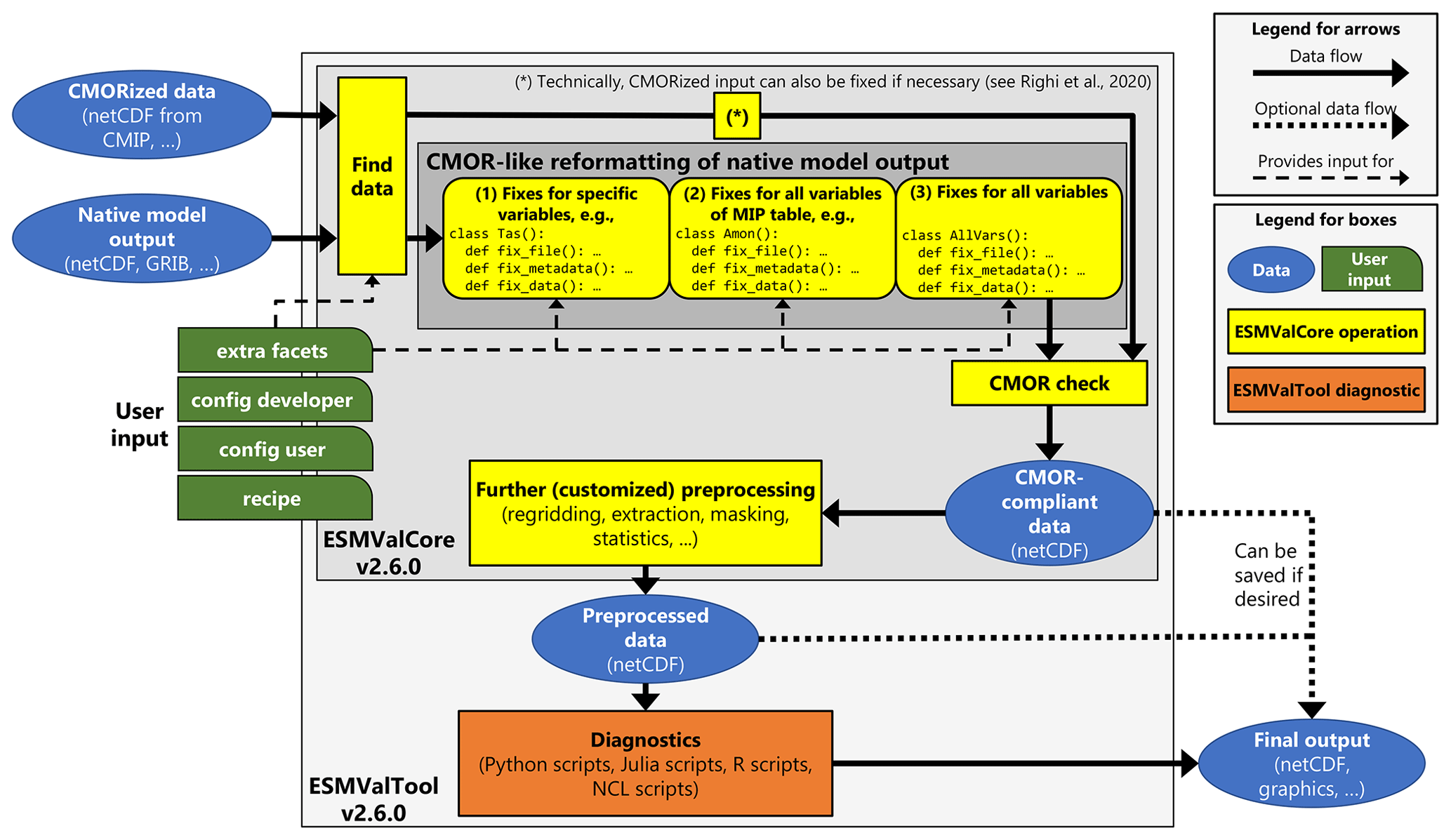
Figure 1Schematic representation of ESMValTool v2.6.0. Originally, ESMValTool was designed to process CMORized output from CMIP (top left blue ellipse). Here, we describe additions that allow reading and processing native model output (bottom left blue ellipse) with ESMValTool through a CMOR-like reformatting (yellow round rectangles) within the ESMValCore preprocessing pipeline. As a result, the data are fully CMOR-compliant after this initial preprocessing step and can be processed by the diagnostic scripts (orange box) just like any other input dataset. The diagnostic scripts do not need to treat native model output in any special way. Note that to reduce the complexity of this schematic, only those dashed arrows that are relevant for this paper are shown.
ESMValTool expects a specific format for names of input files and directories (Data Reference Syntax,
DRS; e.g., Taylor et al., 2021). Default values for these naming conventions are specified in the file
config-developer.yml (green box on the left in Fig. 1). However,
by using a custom config-developer.yml file, arbitrary DRS formats for input files and
directories can be considered. These input conventions can be configured separately for each supported
“project”. In this context, a project refers to a model intercomparison project
(e.g., CMIP3, CMIP5, CMIP6) or a type of observational product (e.g., OBS, obs4MIPs).
However, since the structure and format of native model output can be very diverse, here
project may also refer to the name of the model in its native format, e.g.,
project: ICON for the ICON model. Note that while for projects like CMIP6 or OBS the
key dataset refers to the name of the model or observational product, for native model
output it refers to a sub version of the model or simply repeats the name from the project, e.g.,
dataset: ICON for the ICON model. Due to technical reasons, it is not possible to omit
the key dataset, although it may be redundant in some cases.
To facilitate the handling of native model output, ESMValTool now also allows the automatic
addition of extra facets to the variable metadata (top green box on the left of
Fig. 1). The term “facet” here refers to key-value pairs that describe
datasets requested by the user in an ESMValTool recipe, e.g., project: CMIP6,
dataset: CanESM5, mip: Amon, exp: historical, or
short_name: tas. These extra facets are automatically added to the original facets
(if not already present) depending on the project, dataset name, MIP table, and variable
requested by the user. By default, extra facets are read from a YAML file
contained in the ESMValTool repository. If needed, a custom location
for this file can be specified by the user. An example of extra facets for the EMAC model is
given in Appendix A. In the context of reading native model output, extra facets
can be used to locate input data. For example, if native model output is structured in
subdirectories, the name of the corresponding subdirectory for each variable can be conveniently added
through extra facets. This avoids the necessity to include this information in the ESMValTool recipe,
and the users do not need to be familiar with the peculiarities of each model.
In addition, extra facets are also directly passed to the fix classes mentioned above. This can
be used to further configure the fix operations applied to the data without alterations of the code.
2.2 Supported models
Currently, ESMValTool supports the CMOR-like reformatting of native model output for five different models: CESM2, EC-Earth3, EMAC, ICON, and IPSL-CM6. Detailed user instructions on this can be found in ESMValTool's documentation (ESMValTool Development Team, 2022a). The documentation provides links with further details on all the available models and instructions on how to add support for new climate models.
The following subsections describe details on the implementations of the reformatting procedures for the five currently supported models. All of them fix variable and coordinate metadata (names and units) not compliant with the CMOR standard and add missing scalar coordinates (e.g., 2 m height coordinate for the near-surface air temperature) by default.
2.2.1 CESM2
CESM2 is an ESM developed by the National Center for Atmospheric Research (NCAR) in collaboration with a global community of users and developers (Danabasoglu et al., 2020). Like other ESMs, CESM2 is composed of several components: the Community Atmosphere Model, version 6 (CAM6); the Parallel Ocean Program Version 2 (POP2; Danabasoglu et al., 2012); the Community Land Model, version 5 (CLM5; Lawrence et al., 2019); the Los Alamos sea ice model, version 5 (CICE5; Hunke et al., 2015); and the Model for Scale Adaptive River Transport (MOSART; Li et al., 2013). Additionally, CESM2 has the capability to represent the Greenland ice sheet using the Community Ice Sheet Model Version 2.1 (CISM2.1; Lipscomb et al., 2019) and the ocean biogeochemistry using the Marine Biogeochemistry library (MARBL; Long et al., 2021). The coupling between components is achieved through the Common Infrastructure for Modeling the Earth (CIME; Edwards et al., 2022).
Output from CESM2 consists of netCDF files. Configuration of output variables, frequency, sampling (i.e., average, instantaneous, minimum, or maximum), and other aspects can be set by users via namelist files. The output files are time-slice files consisting of the specified variables at the specified frequency. The most common use case is to put monthly averages of many variables into files, with 1 month per file. For CMIP6, the conversion of these native files to CMOR-compliant files was done with a custom tailored workflow based on Python 2 (see Paul et al., 2019 and Mickelson, 2020). In contrast to the other four models presented in this paper, ESMValTool's support for native CESM2 output is still under development and thus considered experimental. Currently, only surface variables (i.e., no three-dimensional variables with a z dimension) are supported.
2.2.2 EC-Earth3
EC-Earth3 is a global climate model developed as part of the EC-Earth consortium (Döscher et al., 2022). The model is composed of several coupled components to describe the atmosphere, ocean, sea ice, land surface, dynamic vegetation, atmospheric composition, ocean biogeochemistry, and the Greenland ice sheet domains. Atmospheric and land dynamics are represented using the European Centre for Medium-Range Weather Forecast's (ECMWF) Integrated Forecast System (IFS) Cycle 36r4 (e.g., Riddaway, 2001), whereas the ocean is simulated using NEMO3.6 (Madec, 2008, 2015; Madec et al., 2017), which integrates LIM3 (Vancoppenolle et al., 2009; Rousset et al., 2015) and PISCES (Aumont et al., 2015) to represent sea ice processes and the ocean biogeochemistry, respectively. Simulation of dynamic vegetation processes is performed by LPJ-GUESS (Smith et al., 2014; Lindeskog et al., 2013). Aerosols and chemical processes are described by TM5 (van Noije et al., 2021) and the Greenland ice sheet is modeled using PISM (Bueler and Brown, 2009; Winkelmann et al., 2011). The coupling of all components is performed using the OASIS3-MCT coupling library (Craig et al., 2017).
EC-Earth3 produces output in netCDF format for the ocean and the sea ice domains, and in GRIB format for the atmosphere and land domains. As part of the standard workflow used to run the model, these data are then post-processed to a CMOR- and CF-compliant netCDF format. For this, the Python package ece2cmor3 (van den Oord, 2017) is used, which contains modules to format output from each of the model components. Thus, a CMOR-like reformatting of the native (i.e., operational) EC-Earth3 output within ESMValTool during runtime is not necessary. Nevertheless, ESMValTool includes several data and metadata fixes for EC-Earth3 to fully correct issues that have not been handled by ece2cmor3 to ensure consistency over experiments.
2.2.3 EMAC
The ECHAM/MESSy Atmospheric Chemistry (EMAC) model is a numerical chemistry and climate model system that includes submodels for tropospheric and middle atmosphere processes and their interactions with the ocean, land, and human influences (Jöckel et al., 2010). It uses the second version of the Modular Earth Submodel System (MESSy2) to link multi-institutional computer codes. The core atmospheric model is the fifth generation European Centre Hamburg general circulation model (ECHAM5; Roeckner et al., 2006). The physics subroutines of the original ECHAM code have been modularized and re-implemented as MESSy submodels and have been continuously further developed. Only the spectral transform core, the flux-form semi-Lagrangian large-scale advection scheme (Lin and Rood, 1996), and the nudging routines for Newtonian relaxation are remaining from ECHAM. In MESSy, the memory, data types, metadata, and output are handled by the infrastructure submodel CHANNEL (Jöckel et al., 2010), which allows a flexible control of the model output via two Fortran namelists. This includes output redirection to create custom tailored output files; the choice of the output file format, output method (e.g., serial vs. parallel netCDF), output precision, and output frequency; and the capability to conduct basic temporal statistical analyses during runtime, i.e., to output in addition (or alternative) to the instantaneous data (i.e., at a specific model time step) the time average, standard deviation, minimum, maximum, event counts, and event averages for the output time interval. Thus, with CHANNEL, a set of model variables (called “objects”) are grouped into a “channel”. Each channel is output at a user-defined frequency as a (time) series of files. Different channels can be output with different frequencies, and objects can be part of multiple channels.
To reformat EMAC data (most commonly provided in netCDF format), many variable-specific fixes are required since a large number of CMOR-type variables are not directly present in the native model output but need to be derived from other variables. For example, the variable “pr” (total precipitation) is calculated as the sum of the large-scale precipitation, convective precipitation, and snowfall. Consequently, a rather large amount of information needs to be provided in the form of extra facets. This includes raw variable names used in EMAC output files (only necessary if they differ from their corresponding CMOR variable names) and information on the EMAC channel (see above). The channel information given by the extra facets file serves as a default value; if a different channel is requested this can be specified in the ESMValTool recipe.
2.2.4 ICON
The ICON (ICOsahedral Non-hydrostatic) modeling framework, developed by the Max Planck Institute for Meteorology (MPI-M), the German Weather Service/Deutscher Wetterdienst (DWD), and partners, provides a unified modeling system for global numerical weather prediction (NWP) and climate modeling (Zängl et al., 2014). The CMOR-like reformatting of ICON output implemented in ESMValTool primarily targets evaluation of climate model simulations but could be extended to NWP simulations in the future. The reformatting has been successfully tested with output from atmosphere-only simulations (ICON-A; Giorgetta et al., 2018) and fully coupled ESM simulations (ICON-ESM, also known as ICON-Ruby; Jungclaus et al., 2022).
ICON model output consists of netCDF files that already provide many CMOR variables in the correct form. Thus, very few variable-specific fixes and additional information in the form of extra facets are required. These extra facets can include raw variable names given in the ICON output files (only necessary if they differ from their corresponding CMOR variable names) and alternative names for the latitude and longitude coordinates (currently only affects the grid cell areas areacella and areacello as these are extracted directly from the ICON grid file).
As shown in Fig. 2a, native ICON model output uses an unstructured grid whose triangular grid cells are derived from a spherical icosahedron by repeated subdivision of the spherical triangular cells into smaller cells (Giorgetta et al., 2018; Wan et al., 2013). Consequently, the CMOR-like reformatting of ICON requires fixing the spatial coordinate that describes this unstructured grid in addition to the latitude and longitude coordinates. If the grid information (latitude and longitude coordinates) is missing in an input file, which can be the case for ICON output depending on the model settings, it is automatically added during the CMOR-like reformatting using the corresponding grid file. This grid file is specified in the global netCDF attributes of the ICON file and is automatically downloaded from MPI-M servers if necessary. For the vertical grid, the ICON reformatting supports the terrain-following hybrid sigma height coordinates that are used by the ICON model (Giorgetta et al., 2018) but also a regular height coordinate that simply describes the altitude of the grid cells. If available in the input file, pressure levels (including bounds) are added to the ESMValTool output files.
To be able to compare native ICON output directly with other models, observational products, or reanalysis data, an additional preprocessing step is usually necessary to interpolate the ICON data to a regular grid. This can be done with ESMValTool's regridding preprocessor, which is described in detail in Sect. 3. However, ICON data can also be regridded by external tools like CDO (Climate Data Operators; Schulzweida, 2021) if needed by the user, since the CMOR-like reformatting also supports ICON data on regular grids. For example, if users require a regridding algorithm available in CDO but currently not supported by ESMValTool, the native model data can be regridded using CDO in an additional post-processing step after running the model before being processed by ESMValTool.
2.2.5 IPSL-CM6
IPSL-CM6A-LR (hereafter IPSL-CM6) is an ESM developed by the Institut Pierre-Simon Laplace Climate Modeling Center. It is composed of the LMDZ atmospheric model version 6A-LR (Hourdin et al., 2020), the ORCHIDEE land surface model (Krinner et al., 2005) version 2.0, and the NEMO ocean model (Madec, 2008, 2015). The latter is based on the stable version 3.6 of NEMO, which includes three major components: the ocean physics model NEMO-OPA (Madec et al., 2017), the sea ice dynamics and thermodynamics model LIM3 (Vancoppenolle et al., 2009; Rousset et al., 2015), and the ocean biogeochemistry model PISCES (Aumont et al., 2015).
IPSL-CM6 uses the XIOS input/output system (Meurdesoif, 2017), which combined with dr2xml (https://github.com/rigoudyg/dr2xml, last access: 1 November 2022) allows production of CMOR-compliant output directly at run time. However, this feature is not yet standard for IPSL-CM6 runs and activated only for simulations contributing to some MIPs. Typically, simulations for IPSL-CM6 development use the native model output format which exists in two versions: “Output” and “Analyse”. The Output format consists of files that include output for a fixed-length period of time (usually 1 month) and for a group of variables (e.g., all atmospheric 3D variables). These files are grouped in directories that contain all periods for one (or more) variable groups. The Analyse format has been introduced to facilitate the analysis of the model: output files in this format include only one variable for a longer time period (up to the entire simulation period). The Analyse format can be requested in addition to the Output format during setup of the model experiment.
Since native IPSL-CM6 output consists of netCDF files that comply to other conventions like CF, only a small number of ESMValTool fixes is necessary for the CMOR-like reformatting of the data. Apart from common fixes that are applied to all native model datasets (adapting variable and coordinate metadata and the addition of scalar coordinates), a fix for an auxiliary time coordinate that is not CMOR-compliant needs to be applied. Extra facets for IPSL-CM6 include raw variable names used in the native IPSL-CM6 output and information about the variable groups and directories used to store the corresponding variables.
Many state-of-the-art ESMs do not use rectilinear or curvilinear horizontal grids for the spatial discretization but instead use unstructured grids. Unstructured grids are usually described by a list of all grid cells using a single spatial dimension. For each grid cell in this list, latitude and longitude values for the central points (representative for the cell “face”) and bounds (cell “nodes”) are specified by additional variables. Grid cells of unstructured grids usually consist of polygons whose number of vertices is different than four. For example, the ICON model (see Sect. 2.2.4) uses triangular grid cells. Unstructured grids offer numerical advantages in terms of scalability and computational efficiency and also often offer a more straightforward implementation of multi-resolution modeling (e.g., nested high-resolution grids in regions of interest).
However, the evaluation of native model output on unstructured grids is challenging: for example, the output of most observations or reanalyses is given on different (regular) grids (which complicates a direct comparison) and most ESMValTool diagnostics therefore expect data on regular grids. For this reason, a regridding preprocessor that is able to interpolate unstructured grids to regular grids is often crucial for evaluation of such native model output. Currently, ESMValTool provides three different regridding schemes that allow regridding from unstructured grids to regular grids: nearest-neighbor, bilinear, and first-order conservative interpolation. While the first scheme supports unstructured data in arbitrary format (the only prerequisite is the existence of latitude and longitude coordinates), the latter two can only be used with data that follows the UGRID (Unstructured Grid) conventions (Jagers et al., 2016). UGRID provides a systematic description of the topology of unstructured meshes (e.g., it clearly defines the connectivity between the cell faces and nodes), which is necessary to perform the more complex regridding operations. Nearest-neighbor interpolation is natively supported by Iris used in the ESMValTool preprocessor. Bilinear and first-order conservative regridding are supported via the iris-esmf-regrid package (https://github.com/SciTools-incubator/iris-esmf-regrid, last access: 1 November 2022), which collects and provides the Earth System Modeling Framework (ESMF; https://earthsystemmodeling.org/regrid/, last access: 1 November 2022) regridding schemes for Iris. The use of iris-esmf-regrid is possible due to an extension of ESMValTool's regridding functionalities that allows the usage of external regridding packages (in addition to native Iris schemes) with arbitrary options.
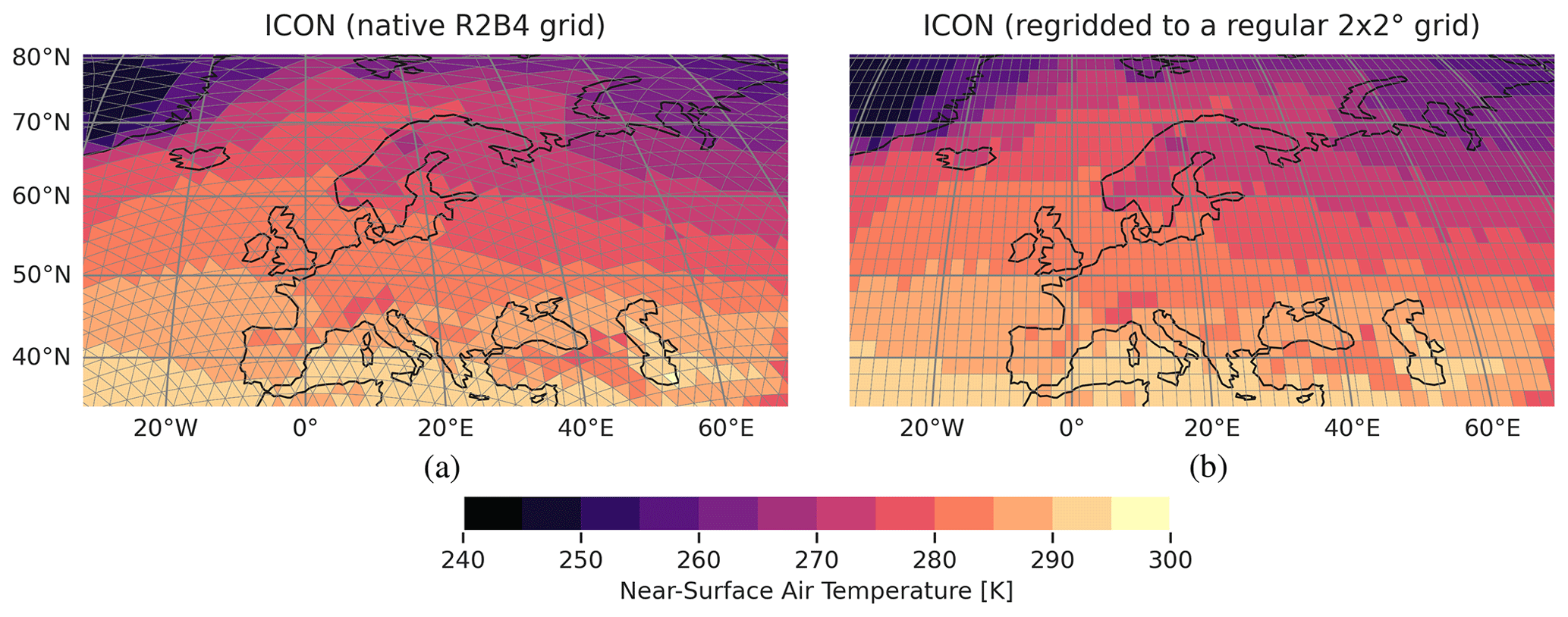
Figure 2Illustration of the regridding of an unstructured grid using the near-surface air temperature climatology over Europe averaged from 1979 to 2014 as an example. The ICON simulation shown here corresponds to the one described in Fig. 3. (a) Native ICON grid at R2B4 resolution (about 160 km). (b) Regular grid that results from ESMValTool's nearest-neighbor regridding of the data shown in (a).
An example of regridding ICON data on an unstructured grid is illustrated by Fig. 2. Figure 2a shows the triangular grid cells of the native model output on an R2B4 grid with a horizontal resolution of about 160 km. Figure 2b shows the data interpolated on a regular grid that has been regridded using ESMValTool's nearest-neighbor scheme. From a visual inspection, both fields are very similar. As an additional sanity check, we calculated the global mean near-surface air temperature for both grids, which gives almost identical values of 287.14 and 287.16 K for the native grid and the interpolated grid, respectively. Since native ICON output does not follow the UGRID conventions, only the nearest-neighbor scheme is currently supported for this model. However, in ESMValTool v2.8.0, the CMOR-like reformatting of ICON will include a first implementation to make ICON output fully UGRID-compliant during runtime of ESMValTool. First tests have shown promising results: the adapted ICON data could be successfully regridded with the first-order conservative algorithm provided by iris-esmf-regrid.
We emphasize that regridding is not a trivial operation in general. ESMValTool's three currently available schemes for unstructured grids are sufficient for many applications; however, this is by no means a complete set of all possible regridding algorithms and does not cover all imaginable applications. For example, variables that describe fractions of quantities within grid cells like land–sea fraction, sea ice concentration, or fractional cloud cover need to be treated with extra care (e.g., Grundner et al., 2022). The nearest-neighbor scheme illustrated in Fig. 2 is sufficient for the purpose of monitoring (i.e., to get a quick overview of simulation results) but should not be used for more sophisticated scientific analyses where precise results are crucial.
One use case of ESMValTool's new capability to process native model output is the near real-time monitoring of running climate model simulations. With this, modeling centers can already check at an early stage whether the output of their simulation appears to be reasonable. Possible problems can be detected very early on, which in turn can save valuable computational resources on supercomputers.
Table 1Overview of the general-purpose monitoring diagnostics implemented in ESMValTool. All diagnostics can handle arbitrary variables from arbitrary datasets.
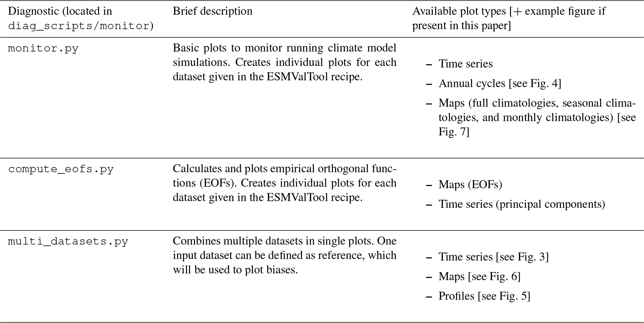
For the purpose of monitoring, a set of general diagnostics has been added to ESMValTool (see
Table 1 for an overview). These diagnostics can be found in the subdirectory
diag_scripts/monitor. All of these diagnostics are able to handle
arbitrary variables from arbitrary datasets, which makes them versatile and flexible to use.
The input for each diagnostic consists of data that have been preprocessed with ESMValTool.
In order to configure the output, a number of parameters can be set and customized in the
ESMValTool recipe that runs the diagnostic script. Settings related to the definition of the
output directories and filenames can also be configured in the ESMValTool recipe in order to store
all output figures in a common location for each simulation following a common naming scheme.
Furthermore, the path to an additional configuration file for the plots is also provided in
the ESMValTool recipe. This configuration file contains map-specific settings for the map
plots (e.g., the map projection) and variable-specific settings (e.g., regions, titles, labels,
and color schemes). Currently, this additional configuration file is only used by the diagnostic
monitor.py.
The general purpose diagnostics are written in Python following an object-oriented implementation
in order to facilitate the extension and inclusion of further monitoring diagnostics. To
illustrate this procedure, the script compute_eofs.py has been developed following the same
structure defined in the main monitor.py script. Since the monitoring diagnostics save their
output according to a customized but structured naming convention, the plot files can be easily used
by other applications, e.g., for visualization. For instance, in the case of monitoring EC-Earth3, an
R Shiny app has been developed in order to conveniently and interactively visualize results by
experiment, realm, and variable. A screenshot of this application is shown in Fig. B1.
Further details on the monitoring diagnostics can be found in ESMValTool's
documentation (ESMValTool Development Team, 2022a).
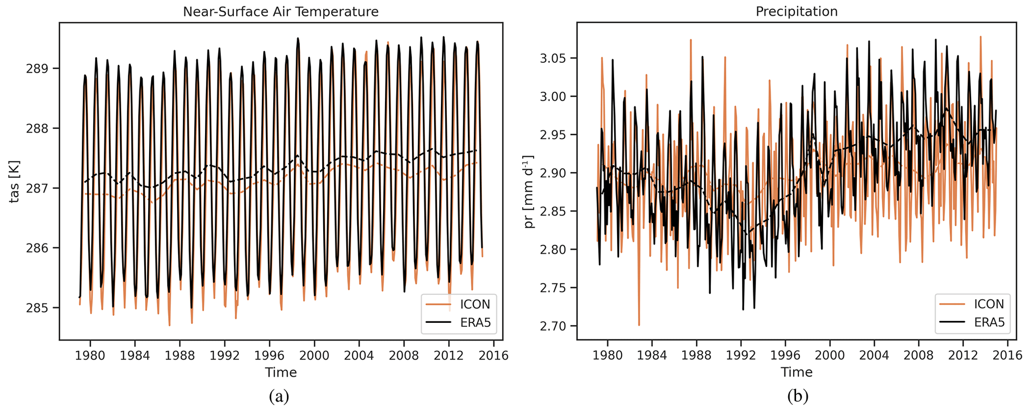
Figure 3Monthly mean (solid lines) and annual mean (dashed lines) time series of ICON-ESM (orange) and ERA5 (black) for the period 1979 to 2014. The ICON simulation shown here (called “Cool Ruby”) is based on a standard AMIP setup at R2B4 resolution (about 160 km) with an advanced representation of soil physics and properties. (a) Global mean near-surface air temperature. (b) Global mean precipitation.
The following paragraphs illustrate five example plots (one for each currently supported climate model) created with these new diagnostics. A recipe to reproduce these figures is publicly available on Zenodo (Schlund, 2022). This recipe showcases the usage of the monitoring diagnostics on native model output and serves as a convenient starting point for users who want to process native model output with ESMValTool.
For a direct comparison with one or multiple reference datasets (e.g., observations,
reanalyses, output from other model versions),
Fig. 3 shows simple time series of the global mean near-surface air
temperature and precipitation from 1979 to 2014 created by the diagnostic multi_datasets.py
for the ESM configuration of ICON (ICON-ESM) and the ERA5 reanalysis (Hersbach et al., 2020).
The ICON simulation shown here is conducted using a standard Atmospheric Model Intercomparison Project
(AMIP) setup at R2B4 resolution (about 160 km). In the CMIP terminology, the AMIP protocol
refers to a simulation of the recent past with all natural and anthropogenic forcings and prescribed
sea surface temperatures and sea ice concentrations (Gates, 1992). Compared to the standard
ICON-ESM setup, this ICON version shown here (called “Cool Ruby”) features an advanced representation
of soil physics and soil properties. This plot type is particularly suited to getting a
quick overview of climate model output and can be used early on in a simulation.
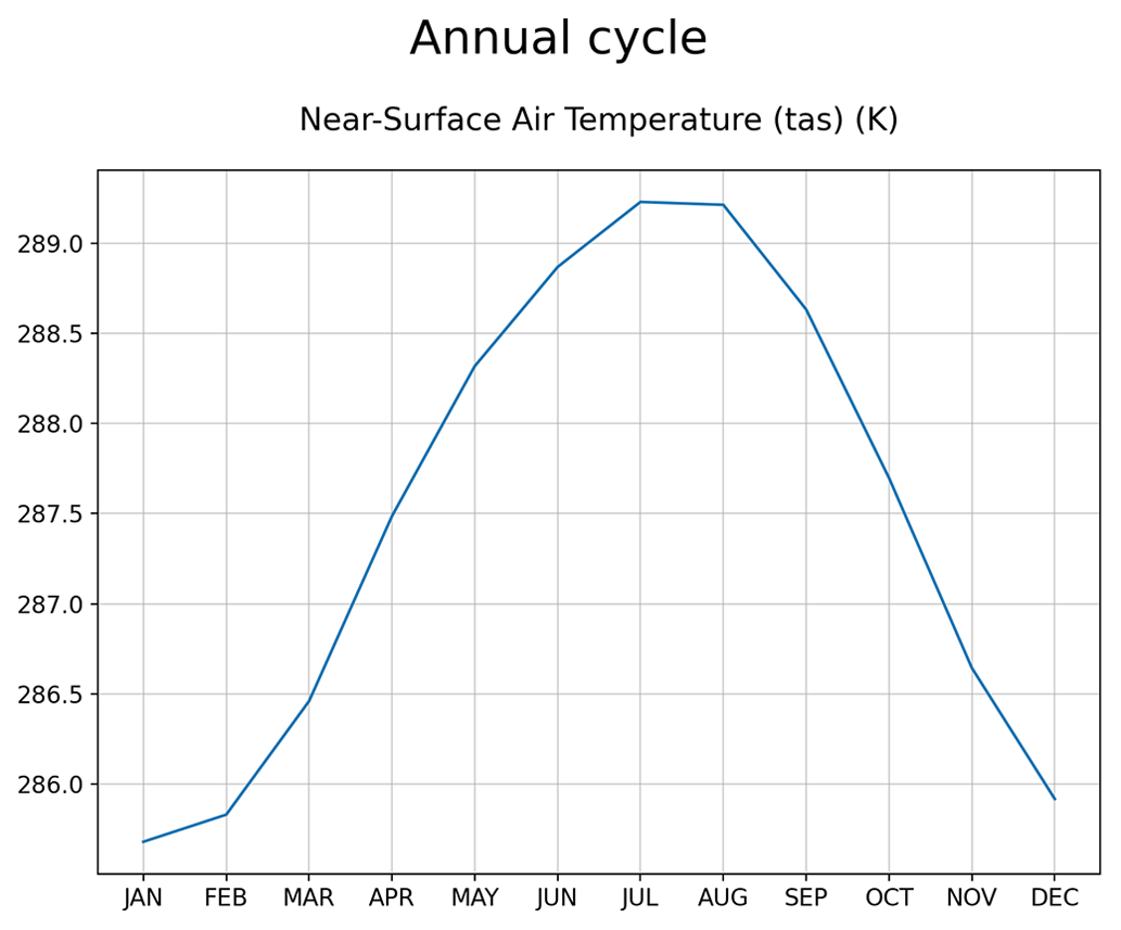
Figure 4Annual cycle of the global mean near-surface air temperature from CESM2 averaged from 2005 to 2014. The CESM2 simulation shown here uses a standard AMIP setup with all forcings from the recent past and prescribed sea surface temperatures and sea ice concentrations.
Apart from such time series, the monitoring diagnostics can also be used to visualize annual
cycles of arbitrary variables. This plot type can be created with the diagnostic monitor.py.
Figure 4 shows an example of this using the annual cycle of the global
mean near-surface air temperature from CESM2. The simulation shown here also uses a standard AMIP setup as
defined by CMIP6 with all forcings (anthropogenic and natural) from the recent past and prescribed sea
surface temperatures and sea ice concentrations.
In addition to the time series shown in Fig. 3, the diagnostic
multi_datasets.py also provides vertical profiles for a model and a reference dataset
including the difference between the two. If no reference dataset is provided, a single vertical
profile of the model is returned. Figure 5 shows an example of the vertical air
temperature profile from EMAC averaged over the years 2005 through 2014. These EMAC results are from
the RC2-base-04 simulation, which is a free running simulation following the Chemistry-Climate
Model Initiative (CCMI-1) protocol (Jöckel et al., 2020). For details about the model setup we refer
to Jöckel et al. (2016). The ERA5 reanalysis is used here as a reference dataset. The top row in
the figure shows the vertical profile from EMAC (left) and ERA5 (right), while the bottom row shows
the bias (calculated as simple difference) between the two datasets.

Figure 5Zonal mean air temperature from EMAC including the bias relative to ERA5 averaged from 2005 to 2014. Numbers in the top left corner correspond to the (area-weighted) average of the fields. Numbers in the top right corner of the bias plots correspond to the (area-weighted) root-mean-square error (RMSE) and the (area-weighted) coefficient of determination (R2) of the EMAC and ERA5 fields. The EMAC results are from the RC2-base-04 simulation (Jöckel et al., 2020), which is a free running simulation following the CCMI-1 protocol (see Jöckel et al., 2016 for details).

Figure 6Global precipitation climatology from EC-Earth3-CC including the bias relative compared to ERA5 averaged over 2005 to 2014. Numbers in the top left corner correspond to the (area-weighted) global average of the fields. Numbers in the top right corner of the bias plots correspond to the (area-weighted) root-mean-square error (RMSE) and the (area-weighted) coefficient of determination (R2) of the EC-Earth3-CC and ERA5 fields. The simulation shown here is an AMIP simulation that has been published as part of the CMIP6 ensemble (ensemble member r1i1p1f1).
Moreover, multi_datasets.py also supports map plots (climatologies).
Just like the vertical profiles provided by this diagnostic, these map plots can also be used to visualize
differences between model data and a reference dataset. As an example, Fig. 6
shows the global precipitation climatology from EC-Earth3-CC averaged over the years 2005 to 2014 in
comparison to the ERA5 reanalysis. The panels are arranged similar to Fig. 5:
the top row shows the climatologies of EC-Earth3-CC (left) and ERA5 (right), and the bottom row the difference
between the two. The EC-Earth3-CC simulation shown is an AMIP simulation that has been
published as part of the CMIP6 ensemble (ensemble member r1i1p1f1).
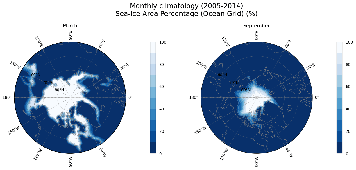
Figure 7March and September Arctic sea ice concentration from IPSL-CM6 averaged over 2005 to 2014. The simulation shown here follows the CMIP6 AMIP protocol.
In contrast to the annual mean climatology given in Fig. 6,
Fig. 7 shows monthly climatologies of the Arctic sea ice concentration
for the months March and September averaged over the years 2005 to 2014 as simulated by IPSL-CM6.
The simulation shown here follows the CMIP6 AMIP protocol. This plot
has been created with monitor.py, which supports arbitrary regions and map projections.
For example, here a stereographic projection is used to focus on the Arctic region.
As mentioned above, the monitoring diagnostics provide further plot types that are not shown here.
This includes (optionally smoothed) time series and seasonal climatologies provided by the
diagnostic monitor.py and empirical orthogonal function (EOF) maps and time series provided
by the diagnostic compute_eofs.py.
The monitoring functionality described in the previous section of this paper is one possible application of ESMValTool's CMOR-like reformatting of native model output. In principle, the rich collection of diagnostics provided by ESMValTool (see the orange box in Fig. 1) is now fully available for all supported models. This includes all diagnostics described in the scientific documentation of ESMValTool, e.g., large-scale diagnostics for a comprehensive evaluation of ESMs (Eyring et al., 2020), diagnostics for emergent constraints and future projections (Lauer et al., 2020), and diagnostics for extreme events, and regional and impact evaluation (Weigel et al., 2021). Moreover, many new diagnostics have been added or will be added to ESMValTool, for example, diagnostics and recipes that have been used to compile parts of the latest Assessment Report 6 (AR6) of the Intergovernmental Panel on Climate Change (IPCC; e.g., Eyring et al., 2021). Since preprocessed output by ESMValTool is fully CMOR-compliant for all input datasets (see Fig. 1), no specific changes to these diagnostic scripts are required when dealing with native model output.
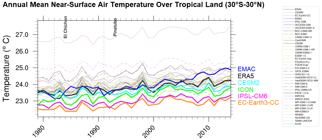
Figure 8Example of an analysis of native model output alongside CMIP data and reanalysis products with ESMValTool's wide range of diagnostics, similar to Fig. 1 of Bock et al. (2020). Annual near-surface air temperature between 1979 and 2014 averaged over tropical land region (30∘ S–30∘ N) for an ensemble of (CMORized) CMIP6 models (thin lines), the ERA5 reanalysis (thick black line), and the models presented in this paper for which a CMOR-like reformatting is available (CESM2: thick cyan line; EMAC: thick blue line; ICON: thick green line; IPSL-CM6: thick magenta line; EC-Earth3-CC: thick orange line). Vertical dashed lines show large volcanic eruptions. For all CMIP6 models and the native output of the models CESM2, EC-Earth3-CC, ICON, and IPSL-CM6, results of an AMIP simulation as defined by CMIP6 (Eyring et al., 2016) are used. The EMAC results shown here are based on a free running EMAC simulation following the CCMI-1 protocol that also uses prescribed sea surface temperatures and sea ice concentrations but a different set of forcings (Jöckel et al., 2016). Due to different model setups, a fair comparison of the individual models is not possible.
As an example, Fig. 8 shows the annual mean near-surface air temperature between 1979 and 2014 averaged over the tropical land region (30∘ S–30∘ N) from the five models described in this paper that have been processed in their native format and an ensemble of (CMORized) CMIP6 models and the ERA5 reanalysis. A similar version of this plot was originally published by Bock et al. (2020) to evaluate progress across different CMIP generations (CMIP3, CMIP5, and CMIP6). All datasets show the steady increase of the near-surface air temperature over the last decades. For all CMIP6 models and the native output of the models CESM2, EC-Earth3-CC, ICON, and IPSL-CM6, this figure shows results of AMIP experiments. The native EMAC output shown here is from a free running EMAC simulation following the CCMI-1 protocol that also uses an AMIP-like setup with a different set of forcings (Jöckel et al., 2016). Figure 8 is just an example, and we would like to note that a fair comparison between the different results shown here is not possible because of the different model setups used. The main aim of this figure is to showcase the evaluation of native model output alongside CMIP data and reanalysis products with ESMValTool's large collection of diagnostics.
The diagnostics presented in Sects. 4 and 5 showcase two example applications possible with ESMValTool's new CMOR-like reformatting of native model output. Further applications are, for example, comparison of newly developed model versions or setups with predecessor versions or observations, or the plain CMORization of native model output prior to publication of the data as a contribution to model intercomparison projects like CMIP.
We have described recent changes and additions to ESMValTool that allow reading and processing native (i.e., operational) model output through an automatic CMOR-like reformatting during runtime for five different climate models: CESM2, EC-Earth3, EMAC, ICON, and IPSL-CM6. Prior to these changes, ESMValTool could only be used with model output that had already been processed to the CMOR standard such as from model intercomparison projects like CMIP. Extending ESMValTool enables the evaluation of native model output and potentially offers a simplified workflow for the CMORization process. This allows ESMValTool to be used during model development or for analysis of non-MIP-related experiments.
Software tools that allow for an easy and comprehensive evaluation of ESMs are increasingly crucial as models continue to increase in complexity and resolution. ESMValTool provides one such tool that enables comparison with observations, reanalyses, and/or other models. The changes to ESMValTool described here are designed to lower the barrier to its use for a broad array of applications.
Along with CMOR-like data processing, ESMValTool provides regridding functionality that allows the use of flexible interpolation schemes and extends the number of available algorithms that can be used on unstructured data. In total, three schemes to interpolate unstructured grids to regular grids are now available: nearest-neighbor, bilinear, and first-order conservative regridding. While the first algorithm supports unstructured data in arbitrary format, the latter two can only be used with UGRID-compliant data. The only model that uses an unstructured grid described in this paper is ICON. Since native ICON output does not follow the UGRID standard, it can only be regridded with the nearest-neighbor algorithm in ESMValTool v2.6.0. While this is sufficient to get a quick overview of simulation results (e.g., for monitoring of running simulations), more sophisticated schemes are needed for scientific analyses. An experimental fix to make ICON output fully UGRID-compliant during runtime has already been implemented in the ESMValTool development version and is expected to be included in future releases of ESMValTool. A number of CMIP models use unstructured grids already (e.g., E3SM, GFDL), and other models (including CESM) are likely to use unstructured grids in future versions. Global high-resolution models (e.g., participating in DYAMOND; Stevens et al., 2019) overwhelmingly use unstructured grids. Therefore, developing these regridding capabilities within ESMValTool anticipates future challenges of model evaluation and intercomparison.
The automatic CMOR-like reformatting of native model output amplifies the application of ESMValTool's wide range of diagnostics. Section 4, for example, demonstrates how ESMValTool can be used to monitor climate model simulations while they are running. For this, new diagnostics have been implemented that handle arbitrary variables from arbitrary datasets. Monitoring of running simulations facilitates the production process at modeling institutes as problems with simulations can be promptly detected. Another example is provided in Sect. 5, showcasing how multiple models in their native format can be easily compared with CMIP6 and reanalysis data. A further expected application of the CMOR-like reformatting is the performance assessment of new model versions or setups. For example, experiments with new parameterizations can be compared to versions of the same model with the previous parameterization scheme to assess the impact on the climate. The CMOR-like reformatting of ESMValTool can also be used simply as a CMORization of the native model output by specifying to save preprocessor output to disk. This can be particularly helpful if the model data needs to be made available in CMORized form, as, for example, required by CMIP for publication of the data to the ESGF (Earth System Grid Federation) servers.
Future developments of ESMValTool will include optimizations of its parallelization capabilities and memory usage, which will allow ESMValTool to process high-resolution data provided by many modern climate models, potentially in their native format. Moreover, the implementation of the CMOR-like reformatting of native model output described in this paper is intentionally kept general and can in principle be applied to any climate model output. The five models presented here serve as examples and can be seen as a starting point for extending ESMValTool's support for native model output. As ESMValTool is an open-source community-driven software tool, contributions from other modeling groups are always very welcome.
# File emac-mappings-example.yml
---
EMAC:  # dataset name
  Amon:  # MIP table
    tas:  # CMOR variable
      raw_name: [temp2_cav, temp2_ave]
      channel: Amon
    ta:  # defined on plev19
      raw_name: [tm1_p19_cav, tm1_p19_ave]
      channel: Amon
  CFmon:
    ta:  # defined on hybrid levels
      raw_name: [tm1_cav, tm1_ave]
      channel: Amon
  Omon:
    tos:
      raw_name: tsw
      channel: g3b
  '*':  # wildcards also work
    '*':
      postproc_flag: ''
The YAML file above (emac-mappings-example.yml) showcases an example of an extra facets
file. It contains small parts of the original extra facets file used to read native EMAC output.
These files are project-specific, i.e., they describe extra facets for all datasets of a given project
defined by the name of the extra facets file (here: EMAC).
Extra facets files consist of nested dictionaries with four layers. The first layer describes the name of the dataset (here: EMAC). The second and third layer correspond to the name of the MIP table (e.g., Amon) and the CMOR variable (e.g., tas), respectively. Finally, the fourth layer lists the facets that will be added to all datasets defined in the ESMValTool recipe that match the description given by the other layers. The key–value pairs given in this fourth layer are model specific. For example, in the EMAC file given here, possible values are the raw variable name used in the EMAC netCDF files (raw_name), the channel name of the variable (channel), and a post-processing flag that can be used to identify EMAC output files that have already been post-processed by an additional script by the modeler (postproc_flag). For the first three layers, wildcards are accepted, which can be used to conveniently add extra facets for multiple datasets, MIP tables, or variables at once.

Figure B1Screenshot of the R Shiny app that has been developed to conveniently and interactively visualize the results of EC-Earth3 simulation output.
The new extensions described in this paper have been available since ESMValTool v2.6.0. ESMValTool v2 is released under the Apache License, version 2.0. The latest release of ESMValTool v2 is publicly available on Zenodo at https://doi.org/10.5281/zenodo.3401363 (Andela et al., 2022a). The source code of the ESMValCore package, which is installed as a dependency of ESMValTool v2, is also publicly available on Zenodo at https://doi.org/10.5281/zenodo.3387139 (Andela et al., 2022b). ESMValTool and ESMValCore are developed on the GitHub repositories available at https://github.com/ESMValGroup (last access: 1 November 2022). An example recipe to get started with processing native model output with ESMValTool is publicly available on Zenodo at https://doi.org/10.5281/zenodo.7254312 (Schlund, 2022). This recipe reproduces Figs. 2–7 of this paper. Detailed user instructions on the CMOR-like reformatting of native model output can be found in ESMValTool's documentation at https://docs.esmvaltool.org/en/latest/input.html#datasets-in-native-format (ESMValTool Development Team, 2022a). The documentation is recommended as a starting point for new users and provides links with further details on all currently supported models and instructions on how to add support for new climate models. For further details, we refer to the general ESMValTool documentation available at https://docs.esmvaltool.org/ (ESMValTool Development Team, 2022a) and the ESMValTool website (https://www.esmvaltool.org/, ESMValTool Development Team, 2022b).
CMIP6 model output (AMIP simulations, Fig. 8), CESM2 output (AMIP simulation, Figs. 4 and 8), EC-Earth3-CC output (AMIP simulation, Figs. 6 and 8), and IPSL-CM6 output (AMIP simulation, Figs. 7 and 8) are available through the Earth System Grid Foundation (ESGF) under https://esgf-data.dkrz.de/projects/esgf-dkrz/ (ESGF, 2022). EMAC output (RD2-base-04 simulation, Fig. 5) is available from the CERA database at the German Climate Computing Center (DKRZ) under https://doi.org/10.26050/WDCC/RC2 (Jöckel et al., 2020). ICON output (Figs. 2, 3, and 8) used in this study is not publicly available. It is based on an intermediate model version and merely used to evaluate the state of development. Is not considered to contain enough scientific value to merit a data publication on its own; however, it can be provided upon request.
MS designed the concept of this study; led the writing of the paper; implemented the CMOR-like reformatting for CESM2, EMAC, and ICON; and contributed to the monitoring diagnostics. BH, AL, and VE contributed to the concept of this study. BA promoted the idea of using the fix system of ESMValTool v2 for fixing native model data. PJ provided EMAC data. SLT provided EC-Earth3 data and designed the monitoring diagnostics. BM provided CESM2 data. SS implemented the CMOR-like reformatting for IPSL-CM6 and provided IPSL-CM6 data. JS provided IPSL-CM6 data. TS provided ICON data. JVR designed the fixes system of ESMValTool v2 and designed the monitoring diagnostics. KZ implemented the extended regridding functionalities presented in this study. MS, BH, AL, BA, RK, SLT, VP, SS, JVR, KZ, and VE contributed to the development of ESMValTool v2. All authors contributed to the text.
At least one of the (co-)authors is a member of the editorial board of Geoscientific Model Development. The peer-review process was guided by an independent editor, and the authors have also no other competing interests to declare.
Publisher's note: Copernicus Publications remains neutral with regard to jurisdictional claims in published maps and institutional affiliations.
The development of ESMValTool is supported by the projects “Climate-Carbon Interactions in the Current Century” (4C; grant agreement no. 821003), “Earth System Models for the Future” (ESM2025; grant agreement no. 101003536), “Infrastructure for the European Network for Earth System Modelling - Phase 3” (IS-ENES3; grant agreement no. 824084), and the European Research Council (ERC) Synergy Grant “Understanding and Modelling the Earth System with Machine Learning” (USMILE; grant agreement no. 855187) under the European Union's Horizon 2020 Research and Innovation Programme. This study is a contribution to the project S1 of the Collaborative Research Centre TRR 181 “Energy Transfers in Atmosphere and Ocean” funded by the Deutsche Forschungsgemeinschaft (DFG, German Research Foundation) (project no. 274762653). Brian Medeiros acknowledges support by the U.S. Department of Energy (award no. DE-SC0022070), the National Science Foundation (NSF) (IA 1947282), the National Center for Atmospheric Research, which is a major facility sponsored by the NSF (cooperative agreement no. 1852977), and the National Oceanic and Atmospheric Administration (award no. NA20OAR4310392). Tobias Stacke acknowledges funding support from the European Research Council (ERC) under the European Union's Horizon 2020 Programme (grant agreement no. 951288). This work used resources of the Deutsches Klimarechenzentrum (DKRZ) granted by its Scientific Steering Committee (WLA) under the project IDs bd0854, bd1179, and id0853. We acknowledge the World Climate Research Programme (WCRP), which, through its Working Group on Coupled Modeling, coordinated and promoted CMIP6. We thank the climate modeling groups for producing and making their model output available, the Earth System Grid Federation (ESGF) for archiving the data and providing access, and the multiple funding agencies who support CMIP and ESGF. We would like to thank Mattia Righi (DLR) for providing helpful comments about the manuscript.
This research has been supported by the H2020 Societal Challenges (grant nos. 821003 and 101003536), H2020 Excellent Science (grant nos. 855187, 951288, and 824084) programmes, and Deutsche Forschungsgemeinschaft DFG (project no. 274762653). Brian Medeiros was supported by the U.S. Department of Energy (award no. DE-SC0022070), the National Science Foundation (NSF) (IA 1947282), the National Center for Atmospheric Research,
which is a major facility sponsored by the NSF (cooperative agreement no. 1852977), and the
National Oceanic and Atmospheric Administration (award no. NA20OAR4310392).
The article processing charges for this open-access publication were covered by the German Aerospace Center (DLR).
This paper was edited by Fiona O'Connor and reviewed by two anonymous referees.
Andela, B., Broetz, B., de Mora, L., Drost, N., Eyring, V., Koldunov, N., Lauer, A., Mueller, B., Predoi, V., Righi, M., Schlund, M., Vegas-Regidor, J., Zimmermann, K., Adeniyi, K., Arnone, E., Bellprat, O., Berg, P., Bock, L., Caron, L.-P., Carvalhais, N., Cionni, I., Cortesi, N., Corti, S., Crezee, B., Davin, E. L., Davini, P., Deser, C., Diblen, F., Docquier, D., Dreyer, L., Ehbrecht, C., Earnshaw, P., Gier, B., Gonzalez-Reviriego, N., Goodman, P., Hagemann, S., von Hardenberg, J., Hassler, B., Hunter, A., Kadow, C., Kindermann, S., Koirala, S., Lledó, L., Lejeune, Q., Lembo, V., Little, B., Loosveldt-Tomas, S., Lorenz, R., Lovato, T., Lucarini, V., Massonnet, F., Mohr, C. W., Moreno-Chamarro, E., Amarjiit, P., Pérez-Zanón, N., Phillips, A., Russell, J., Sandstad, M., Sellar, A., Senftleben, D., Serva, F., Sillmann, J., Stacke, T., Swaminathan, R., Torralba, V., Weigel, K., Roberts, C., Kalverla, P., Alidoost, S., Verhoeven, S., Vreede, B., Smeets, S., Soares Siqueira, A., and Kazeroni, R.: ESMValTool, Zenodo [code], https://doi.org/10.5281/zenodo.6900341, 2022a. a, b
Andela, B., Broetz, B., de Mora, L., Drost, N., Eyring, V., Koldunov, N., Lauer, A., Predoi, V., Righi, M., Schlund, M., Vegas-Regidor, J., Zimmermann, K., Bock, L., Diblen, F., Dreyer, L., Earnshaw, P., Hassler, B., Little, B., Loosveldt-Tomas, S., Smeets, S., Camphuijsen, J., Gier, B. K., Weigel, K., Hauser, M., Kalverla, P., Galytska, E., Cos-Espuña, P., Pelupessy, I., Koirala, S., Stacke, T., Alidoost, S., Jury, M., Sénési, S., Crocker, T., Vreede, B., Soares Siqueira, A., and Kazeroni, R.: ESMValCore, Zenodo [code], https://doi.org/10.5281/zenodo.6838798, 2022b. a
Aumont, O., Ethé, C., Tagliabue, A., Bopp, L., and Gehlen, M.: PISCES-v2: an ocean biogeochemical model for carbon and ecosystem studies, Geosci. Model Dev., 8, 2465–2513, https://doi.org/10.5194/gmd-8-2465-2015, 2015. a, b
Bock, L., Lauer, A., Schlund, M., Barreiro, M., Bellouin, N., Jones, C., Meehl, G. A., Predoi, V., Roberts, M. J., and Eyring, V.: Quantifying Progress Across Different CMIP Phases With the ESMValTool, J. Geophys. Res.-Atmos., 125, e2019JD032321, https://doi.org/10.1029/2019JD032321, 2020. a, b, c
Bueler, E. and Brown, J.: Shallow shelf approximation as a “sliding law” in a thermodynamically coupled ice sheet model, J. Geophys. Res., 114, F03008, https://doi.org/10.1029/2008JF001179, 2009. a
Craig, A., Valcke, S., and Coquart, L.: Development and performance of a new version of the OASIS coupler, OASIS3-MCT_3.0, Geosci. Model Dev., 10, 3297–3308, https://doi.org/10.5194/gmd-10-3297-2017, 2017. a
Danabasoglu, G., Bates, S. C., Briegleb, B. P., Jayne, S. R., Jochum, M., Large, W. G., Peacock, S., and Yeager, S. G.: The CCSM4 Ocean Component, J. Climate, 25, 1361–1389, 2012. a
Danabasoglu, G., Lamarque, J.-F., Bacmeister, J., Bailey, D. A., DuVivier, A. K., Edwards, J., Emmons, L. K., Fasullo, J., Garcia, R., Gettelman, A., Hannay, C., Holland, M. M., Large, W. G., Lauritzen, P. H., Lawrence, D. M., Lenaerts, J. T. M., Lindsay, K., Lipscomb, W. H., Mills, M. J., Neale, R., Oleson, K. W., Otto-Bliesner, B., Phillips, A. S., Sacks, W., Tilmes, S., van Kampenhout, L., Vertenstein, M., Bertini, A., Dennis, J., Deser, C., Fischer, C., Fox-Kemper, B., Kay, J. E., Kinnison, D., Kushner, P. J., Larson, V. E., Long, M. C., Mickelson, S., Moore, J. K., Nienhouse, E., Polvani, L., Rasch, P. J., and Strand, W. G.: The Community Earth System Model Version 2 (CESM2), J. Adv. Model. Earth Sy., 12, e2019MS001916, https://doi.org/10.1029/2019MS001916, 2020. a
Dask Development Team: Dask: Library for dynamic task scheduling, https://dask.org (last access: 1 November 2022), 2016. a
Döscher, R., Acosta, M., Alessandri, A., Anthoni, P., Arsouze, T., Bergman, T., Bernardello, R., Boussetta, S., Caron, L.-P., Carver, G., Castrillo, M., Catalano, F., Cvijanovic, I., Davini, P., Dekker, E., Doblas-Reyes, F. J., Docquier, D., Echevarria, P., Fladrich, U., Fuentes-Franco, R., Gröger, M., v. Hardenberg, J., Hieronymus, J., Karami, M. P., Keskinen, J.-P., Koenigk, T., Makkonen, R., Massonnet, F., Ménégoz, M., Miller, P. A., Moreno-Chamarro, E., Nieradzik, L., van Noije, T., Nolan, P., O'Donnell, D., Ollinaho, P., van den Oord, G., Ortega, P., Prims, O. T., Ramos, A., Reerink, T., Rousset, C., Ruprich-Robert, Y., Le Sager, P., Schmith, T., Schrödner, R., Serva, F., Sicardi, V., Sloth Madsen, M., Smith, B., Tian, T., Tourigny, E., Uotila, P., Vancoppenolle, M., Wang, S., Wårlind, D., Willén, U., Wyser, K., Yang, S., Yepes-Arbós, X., and Zhang, Q.: The EC-Earth3 Earth system model for the Coupled Model Intercomparison Project 6, Geosci. Model Dev., 15, 2973–3020, https://doi.org/10.5194/gmd-15-2973-2022, 2022. a
Eaton, B., Gregory, J., Drach, B., Taylor, K., Hankin, S., Blower, J., Caron, J., Signell, R., Bentley, P., Rappa, G., Höck, H., Pamment, A., Juckes, M., Raspaud, M., Horne, R., Whiteaker, T., Blodgett, D., Zender, C., Lee, D., Hassell, D., Snow, A. D., Kölling, T., Allured, D., Jelenak, A., Soerensen, A. M., Gaultier, L., and Herlédan, S.: NetCDF Climate and Forecast (CF) Metadata Conventions Version 1.10, https://cfconventions.org/Data/cf-conventions/cf-conventions-1.10/cf-conventions.pdf, last access: 1 November 2022. a
Edwards, J., Foucar, J., Bertini, A., Boutte, J., Craig, T., Deakin, M., Fischer, C., Foster, E., Goldhaber, S., Jacob, R., Levy, M., Sacks, B., Salinger, A., Santos, S., Sarich, J., Vertenstein, M., and Wilke, A.: CIME – Common Infrastructure for Modeling the Earth, GitHub, https://github.com/ESMCI/cime, last access: 1 November 2022. a
ESGF: ESGF Node at DKRZ, https://esgf-data.dkrz.de/projects/esgf-dkrz/, last access: 1 November 2022. a
ESMValTool Development Team: ESMValTool Documentation, https://docs.esmvaltool.org, last access: 1 November 2022a. a, b, c, d
ESMValTool Development Team: ESMValTool Website, https://www.esmvaltool.org/, last access: 1 November 2022b. a
Eyring, V., Bony, S., Meehl, G. A., Senior, C. A., Stevens, B., Stouffer, R. J., and Taylor, K. E.: Overview of the Coupled Model Intercomparison Project Phase 6 (CMIP6) experimental design and organization, Geosci. Model Dev., 9, 1937–1958, https://doi.org/10.5194/gmd-9-1937-2016, 2016. a, b, c
Eyring, V., Cox, P. M., Flato, G. M., Gleckler, P. J., Abramowitz, G., Caldwell, P., Collins, W. D., Gier, B. K., Hall, A. D., Hoffman, F. M., Hurtt, G. C., Jahn, A., Jones, C. D., Klein, S. A., Krasting, J. P., Kwiatkowski, L., Lorenz, R., Maloney, E., Meehl, G. A., Pendergrass, A. G., Pincus, R., Ruane, A. C., Russell, J. L., Sanderson, B. M., Santer, B. D., Sherwood, S. C., Simpson, I. R., J., S. R., and Williamson, M. S.: Taking climate model evaluation to the next level, Nat. Clim. Change, 9, 102–110, https://doi.org/10.1038/s41558-018-0355-y, 2019. a
Eyring, V., Bock, L., Lauer, A., Righi, M., Schlund, M., Andela, B., Arnone, E., Bellprat, O., Brötz, B., Caron, L.-P., Carvalhais, N., Cionni, I., Cortesi, N., Crezee, B., Davin, E. L., Davini, P., Debeire, K., de Mora, L., Deser, C., Docquier, D., Earnshaw, P., Ehbrecht, C., Gier, B. K., Gonzalez-Reviriego, N., Goodman, P., Hagemann, S., Hardiman, S., Hassler, B., Hunter, A., Kadow, C., Kindermann, S., Koirala, S., Koldunov, N., Lejeune, Q., Lembo, V., Lovato, T., Lucarini, V., Massonnet, F., Müller, B., Pandde, A., Pérez-Zanón, N., Phillips, A., Predoi, V., Russell, J., Sellar, A., Serva, F., Stacke, T., Swaminathan, R., Torralba, V., Vegas-Regidor, J., von Hardenberg, J., Weigel, K., and Zimmermann, K.: Earth System Model Evaluation Tool (ESMValTool) v2.0 – an extended set of large-scale diagnostics for quasi-operational and comprehensive evaluation of Earth system models in CMIP, Geosci. Model Dev., 13, 3383–3438, https://doi.org/10.5194/gmd-13-3383-2020, 2020. a, b
Eyring, V., Gillett, N., Achutarao, K., Barimalala, R., Barreiro Parrillo, M., Bellouin, N., Cassou, C., Durack, P., Kosaka, Y., McGregor, S., Min, S., Morgenstern, O., and Sun, Y.: Human Influence on the Climate System: Contribution of Working Group I to the Sixth Assessment Report of the Intergovernmental Panel on Climate Change, IPCC Sixth Assessment Report, https://www.ipcc.ch/report/ar6/wg1/downloads/report/IPCC_AR6_WGI_Chapter03.pdf (last access: 1 November 2022), 2021. a
Gates, W. L.: AN AMS CONTINUING SERIES: GLOBAL CHANGE–AMIP: The Atmospheric Model Intercomparison Project, B. Am. Meteorol. Soc., 73, 1962–1970, https://doi.org/10.1175/1520-0477(1992)073<1962:ATAMIP>2.0.CO;2, 1992. a
Giorgetta, M. A., Brokopf, R., Crueger, T., Esch, M., Fiedler, S., Helmert, J., Hohenegger, C., Kornblueh, L., Köhler, M., Manzini, E., Mauritsen, T., Nam, C., Raddatz, T., Rast, S., Reinert, D., Sakradzija, M., Schmidt, H., Schneck, R., Schnur, R., Silvers, L., Wan, H., Zängl, G., and Stevens, B.: ICON-A, the Atmosphere Component of the ICON Earth System Model: I. Model Description, J. Adv. Model. Earth Sy., 10, 1613–1637, https://doi.org/10.1029/2017MS001242, 2018. a, b, c
Grundner, A., Beucler, T., Gentine, P., Iglesias-Suarez, F., Giorgetta, M. A., and Eyring, V.: Deep learning based cloud cover parameterization for ICON, J. Adv. Model. Earth Sy., 14, e2021MS002959, https://doi.org/10.1029/2021MS002959, 2022. a
Hersbach, H., Bell, B., Berrisford, P., Hirahara, S., Horányi, A., Muñoz-Sabater, J., Nicolas, J., Peubey, C., Radu, R., Schepers, D., Simmons, A., Soci, C., Abdalla, S., Abellan, X., Balsamo, G., Bechtold, P., Biavati, G., Bidlot, J., Bonavita, M., De Chiara, G., Dahlgren, P., Dee, D., Diamantakis, M., Dragani, R., Flemming, J., Forbes, R., Fuentes, M., Geer, A., Haimberger, L., Healy, S., Hogan, R. J., Hólm, E., Janisková, M., Keeley, S., Laloyaux, P., Lopez, P., Lupu, C., Radnoti, G., de Rosnay, P., Rozum, I., Vamborg, F., Villaume, S., and Thépaut, J.-N.: The ERA5 global reanalysis, Q. J. Roy. Meteor. Soc., 146, 1999–2049, https://doi.org/10.1002/qj.3803, 2020. a
Hourdin, F., Rio, C., Grandpeix, J.-Y., Madeleine, J.-B., Cheruy, F., Rochetin, N., Jam, A., Musat, I., Idelkadi, A., Fairhead, L., Foujols, M.-A., Mellul, L., Traore, A.-K., Dufresne, J.-L., Boucher, O., Lefebvre, M.-P., Millour, E., Vignon, E., Jouhaud, J., Diallo, F. B., Lott, F., Gastineau, G., Caubel, A., Meurdesoif, Y., and Ghattas, J.: LMDZ6A: The Atmospheric Component of the IPSL Climate Model With Improved and Better Tuned Physics, J. Adv. Model. Earth Sy., 12, e2019MS001892, https://doi.org/10.1029/2019MS001892, 2020. a
Hunke, E. C., Lipscomb, W. H., Turner, A. K., Jeffery, N., and Elliott, S.: CICE: The Los Alamos Sea Ice Model. Documentation and Software User's Manual. Version 5.1, Tech. Rep. LA-CC-06-012, T-3 Fluid Dynamics Group, Los Alamos National Laboratory, https://svn-ccsm-models.cgd.ucar.edu/cesm1/alphas/branches/cesm1_5_alpha04c_timers/components/cice/src/doc/cicedoc.pdf (last access: 1 November 2022), 2015. a
Jagers, B., Stuebe, D., Gross, T., Barker, C., Zelenke, B., Signell, R., Oehmke, B., Crosby, A., Schuchardt, K., Ham, D., Blanton, B., Forbes, C., Seaton, C., Forrest, D., Howe, B., Cowles, G., and Elson, P.: UGRID Conventions (v1.0), GitHub, https://ugrid-conventions.github.io/ugrid-conventions/ (last access: 1 November 2022), 2016. a
Juckes, M., Taylor, K. E., Durack, P. J., Lawrence, B., Mizielinski, M. S., Pamment, A., Peterschmitt, J.-Y., Rixen, M., and Sénési, S.: The CMIP6 Data Request (DREQ, version 01.00.31), Geosci. Model Dev., 13, 201–224, https://doi.org/10.5194/gmd-13-201-2020, 2020. a
Jungclaus, J. H., Lorenz, S. J., Schmidt, H., Brovkin, V., Brüggemann, N., Chegini, F., Crüger, T., De-Vrese, P., Gayler, V., Giorgetta, M. A., Gutjahr, O., Haak, H., Hagemann, S., Hanke, M., Ilyina, T., Korn, P., Kröger, J., Linardakis, L., Mehlmann, C., Mikolajewicz, U., Müller, W. A., Nabel, J. E. M. S., Notz, D., Pohlmann, H., Putrasahan, D. A., Raddatz, T., Ramme, L., Redler, R., Reick, C. H., Riddick, T., Sam, T., Schneck, R., Schnur, R., Schupfner, M., Storch, J.-S., Wachsmann, F., Wieners, K.-H., Ziemen, F., Stevens, B., Marotzke, J., and Claussen, M.: The ICON Earth System Model Version 1.0, J. Adv. Model. Earth Sy., 14, e2021MS002813, https://doi.org/10.1029/2021ms002813, 2022. a
Jöckel, P., Kerkweg, A., Pozzer, A., Sander, R., Tost, H., Riede, H., Baumgaertner, A., Gromov, S., and Kern, B.: Development cycle 2 of the Modular Earth Submodel System (MESSy2), Geosci. Model Dev., 3, 717–752, https://doi.org/10.5194/gmd-3-717-2010, 2010. a, b
Jöckel, P., Tost, H., Pozzer, A., Kunze, M., Kirner, O., Brenninkmeijer, C. A. M., Brinkop, S., Cai, D. S., Dyroff, C., Eckstein, J., Frank, F., Garny, H., Gottschaldt, K.-D., Graf, P., Grewe, V., Kerkweg, A., Kern, B., Matthes, S., Mertens, M., Meul, S., Neumaier, M., Nützel, M., Oberländer-Hayn, S., Ruhnke, R., Runde, T., Sander, R., Scharffe, D., and Zahn, A.: Earth System Chemistry integrated Modelling (ESCiMo) with the Modular Earth Submodel System (MESSy) version 2.51, Geosci. Model Dev., 9, 1153–1200, https://doi.org/10.5194/gmd-9-1153-2016, 2016. a, b, c, d
Jöckel, P., Tost, H., Pozzer, A., Kunze, M., Kirner, O., Brenninkmeijer, C. A. M., Brinkop, S., Cai, D. S., Dyroff, C., Eckstein, J., Frank, F., Garny, H., Gottschaldt, K.-D., Graf, P., Grewe, V., Kerkweg, A., Kern, B., Matthes, S., Mertens, M., Meul, S., Neumaier, M., Nützel, M., Oberländer-Hayn, S., Pfeiffer, A., Ruhnke, R., Runde, T., Sander, R., Scharffe, D., and Zahn, A.: ESCiMo / CCMI: future simulations scenario RCP6.0, SSTs/SICs from coupled HADGEM2-ES simulation and with interactive ocean, respectively, 1960–2100, World Data Center for Climate (WDCC) at DKRZ [data set], https://doi.org/10.26050/WDCC/RC2, 2020. a, b, c
Krinner, G., Viovy, N., de Noblet-Ducoudré, N., Ogée, J., Polcher, J., Friedlingstein, P., Ciais, P., Sitch, S., and Prentice, I. C.: A dynamic global vegetation model for studies of the coupled atmosphere-biosphere system, Global Biogeochem. Cy., 19, GB1015, https://doi.org/10.1029/2003GB002199, 2005. a
Lauer, A., Eyring, V., Bellprat, O., Bock, L., Gier, B. K., Hunter, A., Lorenz, R., Pérez-Zanón, N., Righi, M., Schlund, M., Senftleben, D., Weigel, K., and Zechlau, S.: Earth System Model Evaluation Tool (ESMValTool) v2.0 – diagnostics for emergent constraints and future projections from Earth system models in CMIP, Geosci. Model Dev., 13, 4205–4228, https://doi.org/10.5194/gmd-13-4205-2020, 2020. a, b
Lawrence, D. M., Fisher, R. A., Koven, C. D., Oleson, K. W., Swenson, S. C., Bonan, G., Collier, N., Ghimire, B., van Kampenhout, L., Kennedy, D., Kluzek, E., Lawrence, P. J., Li, F., Li, H., Lombardozzi, D., Riley, W. J., Sacks, W. J., Shi, M., Vertenstein, M., Wieder, W. R., Xu, C., Ali, A. A., Badger, A. M., Bisht, G., van den Broeke, M., Brunke, M. A., Burns, S. P., Buzan, J., Clark, M., Craig, A., Dahlin, K., Drewniak, B., Fisher, J. B., Flanner, M., Fox, A. M., Gentine, P., Hoffman, F., Keppel-Aleks, G., Knox, R., Kumar, S., Lenaerts, J., Leung, L. R., Lipscomb, W. H., Lu, Y., Pandey, A., Pelletier, J. D., Perket, J., Randerson, J. T., Ricciuto, D. M., Sanderson, B. M., Slater, A., Subin, Z. M., Tang, J., Thomas, R. Q., Val Martin, M., and Zeng, X.: The Community Land Model Version 5: Description of New Features, Benchmarking, and Impact of Forcing Uncertainty, J. Adv. Model. Earth Sy., 11, 4245–4287, 2019. a
Li, H., Wigmosta, M. S., Wu, H., Huang, M., Ke, Y., Coleman, A. M., and Leung, L. R.: A Physically Based Runoff Routing Model for Land Surface and Earth System Models, J. Hydrometeorol., 14, 808–828, 2013. a
Lin, S.-J. and Rood, R. B.: Multidimensional Flux-Form Semi-Lagrangian Transport Schemes, Mon. Weather Rev., 124, 2046–2070, https://doi.org/10.1175/1520-0493(1996)124<2046:MFFSLT>2.0.CO;2, 1996. a
Lindeskog, M., Arneth, A., Bondeau, A., Waha, K., Seaquist, J., Olin, S., and Smith, B.: Implications of accounting for land use in simulations of ecosystem carbon cycling in Africa, Earth Syst. Dynam., 4, 385–407, https://doi.org/10.5194/esd-4-385-2013, 2013. a
Lipscomb, W. H., Price, S. F., Hoffman, M. J., Leguy, G. R., Bennett, A. R., Bradley, S. L., Evans, K. J., Fyke, J. G., Kennedy, J. H., Perego, M., Ranken, D. M., Sacks, W. J., Salinger, A. G., Vargo, L. J., and Worley, P. H.: Description and evaluation of the Community Ice Sheet Model (CISM) v2.1, Geosci. Model Dev., 12, 387–424, https://doi.org/10.5194/gmd-12-387-2019, 2019. a
Long, M. C., Moore, J. K., Lindsay, K., Levy, M., Doney, S. C., Luo, J. Y., Krumhardt, K. M., Letscher, R. T., Grover, M., and Sylvester, Z. T.: Simulations With the Marine Biogeochemistry Library (MARBL), J. Adv. Model. Earth Sy., 13, e2021MS002647, https://doi.org/10.1029/2021MS002647, 2021. a
Madec, G.: NEMO ocean engine, Note du Pôle de modélisation, Tech. rep., Institut Pierre-Simon Laplace (IPSL), Paris, France, no. 27, ISSN 1288-1619, 2008. a, b
Madec, G.: The NEMO system team: Nemo ocean engine, version 3.6 stable, Note du Pôle de modélisation, Tech. rep., Institut Pierre-Simon Laplace (IPSL), Paris, France, no. 27, 2015. a, b
Madec, G., Bourdallé-Badie, R., Bouttier, P.-A., Bricaud, C., Bruciaferri, D., Calvert, D., Chanut, J., Clementi, E., Coward, A., Delrosso, D., Ethé, C., Flavoni, S., Graham, T., Harle, J., Iovino, D., Lea, D., Lévy, C., Lovato, T., Martin, N., Masson, S., Mocavero, S., Paul, J., Rousset, C., Storkey, D., Storto, A., and Vancoppenolle, M.: NEMO ocean engine, Zenodo [code], https://doi.org/10.5281/zenodo.1472492, 2017. a, b
Mauzey, C., Durack, P., Taylor, K. E., Florek, P., Doutriaux, C., Nadeau, D., Hogan, E., Kettleborough, J., Weigel, T., kjoti, jmrgonza, Nicholls, Z., Betts, E., Seddon, J., and Wachsmann, F.: PCMDI/CMOR: CMOR v3.7.1, Zenodo [code], https://doi.org/10.5281/zenodo.7379080, 2022. a
Met Office: Iris: A Python library for analysing and visualising meteorological and oceanographic data sets, Exeter, Devon, v1.2 Edn., http://scitools.org.uk/ (last access: 1 November 2022), 2010–2013. a
Meurdesoif, Y.: XIOS 2.0 (Revision 1297), https://doi.org/10.5281/zenodo.4905653, 2017. a
Mickelson, S.: NCAR/conform-input: conform-input version 1.0.0, Zenodo [code], https://doi.org/10.5281/zenodo.3983646, 2020. a
Paul, K., Mickelson, S., and Dennis, J.: PyConform, Zenodo [code], https://doi.org/10.5281/zenodo.3895009, 2019. a
Riddaway, B.: ECMWF Newsletter No. 126 – Winter 2010/11, https://www.ecmwf.int/node/14597 (last access: 1 November 2022), 2001. a
Righi, M., Andela, B., Eyring, V., Lauer, A., Predoi, V., Schlund, M., Vegas-Regidor, J., Bock, L., Brötz, B., de Mora, L., Diblen, F., Dreyer, L., Drost, N., Earnshaw, P., Hassler, B., Koldunov, N., Little, B., Loosveldt Tomas, S., and Zimmermann, K.: Earth System Model Evaluation Tool (ESMValTool) v2.0 – technical overview, Geosci. Model Dev., 13, 1179–1199, https://doi.org/10.5194/gmd-13-1179-2020, 2020. a, b, c
Roeckner, E., Brokopf, R., Esch, M., Giorgetta, M., Hagemann, S., Kornblueh, L., Manzini, E., Schlese, U., and Schulzweida, U.: Sensitivity of Simulated Climate to Horizontal and Vertical Resolution in the ECHAM5 Atmosphere Model, J. Climate, 19, 3771–3791, https://doi.org/10.1175/JCLI3824.1, 2006. a
Rousset, C., Vancoppenolle, M., Madec, G., Fichefet, T., Flavoni, S., Barthélemy, A., Benshila, R., Chanut, J., Levy, C., Masson, S., and Vivier, F.: The Louvain-La-Neuve sea ice model LIM3.6: global and regional capabilities, Geosci. Model Dev., 8, 2991–3005, https://doi.org/10.5194/gmd-8-2991-2015, 2015. a, b
Schlund, M.: Evaluation of Native Earth System Model Output with ESMValTool, Zenodo [code], https://doi.org/10.5281/zenodo.7254313, 2022. a, b
Schulzweida, U.: CDO User Guide, Zenodo [code], https://doi.org/10.5281/zenodo.5614769, 2021. a
Smith, B., Wårlind, D., Arneth, A., Hickler, T., Leadley, P., Siltberg, J., and Zaehle, S.: Implications of incorporating N cycling and N limitations on primary production in an individual-based dynamic vegetation model, Biogeosciences, 11, 2027–2054, https://doi.org/10.5194/bg-11-2027-2014, 2014. a
Stevens, B., Satoh, M., Auger, L., Biercamp, J., Bretherton, C. S., Chen, X., Düben, P., Judt, F., Khairoutdinov, M., Klocke, D., Kodama, C., Kornblueh, L., Lin, S. J., Neumann, P., Putman, W. M., Röber, N., Shibuya, R., Vanniere, B., Vidale, P. L., Wedi, N., and Zhou, L.: DYAMOND: the DYnamics of the Atmospheric general circulation Modeled On Non-hydrostatic Domains, Progr. Earth Planet. Sci., 6, 61, https://doi.org/10.1186/s40645-019-0304-z, 2019. a
Taylor, K. E., Balaji, V., Hankin, S., Juckes, M., Lawrence, B., and Pascoe, S.: CMIP5 Data Reference Syntax (DRS) and Controlled Vocabularies Version 1.3.1, https://pcmdi.llnl.gov/mips/cmip5/docs/cmip5_data_reference_syntax.pdf (last access: 1 November 2022), 2012. a
Vancoppenolle, M., Fichefet, T., Goosse, H., Bouillon, S., Madec, G., and Maqueda, M. A. M.: Simulating the mass balance and salinity of Arctic and Antarctic sea ice. 1. Model description and validation, Ocean Model., 27, 33–53, https://doi.org/10.1016/j.ocemod.2008.10.005, 2009. a, b
van den Oord, G.: ece2cmor3, Zenodo [code], https://doi.org/10.5281/zenodo.1051094, 2017. a
van Noije, T., Bergman, T., Le Sager, P., O'Donnell, D., Makkonen, R., Gonçalves-Ageitos, M., Döscher, R., Fladrich, U., von Hardenberg, J., Keskinen, J.-P., Korhonen, H., Laakso, A., Myriokefalitakis, S., Ollinaho, P., Pérez García-Pando, C., Reerink, T., Schrödner, R., Wyser, K., and Yang, S.: EC-Earth3-AerChem: a global climate model with interactive aerosols and atmospheric chemistry participating in CMIP6, Geosci. Model Dev., 14, 5637–5668, https://doi.org/10.5194/gmd-14-5637-2021, 2021. a
van Rossum, G., Warsaw, B., and Coghlan, N.: PEP 8 – Style Guide for Python Code, https://peps.python.org/pep-0008/ (last access: 1 November 2022), 2001. a
Wan, H., Giorgetta, M. A., Zängl, G., Restelli, M., Majewski, D., Bonaventura, L., Fröhlich, K., Reinert, D., Rípodas, P., Kornblueh, L., and Förstner, J.: The ICON-1.2 hydrostatic atmospheric dynamical core on triangular grids – Part 1: Formulation and performance of the baseline version, Geosci. Model Dev., 6, 735–763, https://doi.org/10.5194/gmd-6-735-2013, 2013. a
Weigel, K., Bock, L., Gier, B. K., Lauer, A., Righi, M., Schlund, M., Adeniyi, K., Andela, B., Arnone, E., Berg, P., Caron, L.-P., Cionni, I., Corti, S., Drost, N., Hunter, A., Lledó, L., Mohr, C. W., Paçal, A., Pérez-Zanón, N., Predoi, V., Sandstad, M., Sillmann, J., Sterl, A., Vegas-Regidor, J., von Hardenberg, J., and Eyring, V.: Earth System Model Evaluation Tool (ESMValTool) v2.0 – diagnostics for extreme events, regional and impact evaluation, and analysis of Earth system models in CMIP, Geosci. Model Dev., 14, 3159–3184, https://doi.org/10.5194/gmd-14-3159-2021, 2021. a, b
Winkelmann, R., Martin, M. A., Haseloff, M., Albrecht, T., Bueler, E., Khroulev, C., and Levermann, A.: The Potsdam Parallel Ice Sheet Model (PISM-PIK) – Part 1: Model description, The Cryosphere, 5, 715–726, https://doi.org/10.5194/tc-5-715-2011, 2011. a
YAML Language Development Team: YAML Ain't Markup Language (YAML) version 1.2, https://yaml.org/ (last access: 1 November 2022), 2021. a
Zängl, G., Reinert, D., Rípodas, P., and Baldauf, M.: The ICON (ICOsahedral Non-hydrostatic) modelling framework of DWD and MPI-M: Description of the non-hydrostatic dynamical core, Q. J. Roy. Meteor. Soc., 141, 563–579, https://doi.org/10.1002/qj.2378, 2014. a
- Abstract
- Introduction
- CMOR-like reformatting of native model output
- Regridding data on unstructured grids
- Monitoring of running climate model simulations
- Availability of ESMValTool's rich set of diagnostics for native model output
- Summary and outlook
- Appendix A: Example extra facets file
- Appendix B: Application to visualize results of monitoring diagnostics
- Code availability
- Data availability
- Author contributions
- Competing interests
- Disclaimer
- Acknowledgements
- Financial support
- Review statement
- References