Testing the reconstruction of modelled particulate organic carbon from surface ecosystem components using PlankTOM12 and machine learning

Understanding the relationship between surface marine ecosystems and the export of carbon to depth by sinking organic particles is key to representing the effect of ecosystem dynamics and diversity, and their evolution under multiple stressors, on the carbon cycle and climate in models. Recent observational technologies have greatly increased the amount of data available, both for the abundance of diverse plankton groups and for the concentration and properties of particulate organic carbon in the ocean interior. Here we use synthetic model data to test the potential of using machine learning (ML) to reproduce concentrations of particulate organic carbon within the ocean interior based on surface ecosystem and environmental data. We test two machine learning methods that differ in their approaches to data-fitting, the random forest and XGBoost methods. The synthetic data are sampled from the PlankTOM12 global biogeochemical model using the time and coordinates of existing observations. We test 27 different combinations of possible drivers to reconstruct small (POC_S) and large (POC_L) particulate organic carbon concentrations. We show that ML can successfully be used to reproduce modelled particulate organic carbon over most of the ocean based on ecosystem and modelled environmental drivers. XGBoost showed better results compared to random forest thanks to its gradient boosting trees' architecture. The inclusion of plankton functional types (PFTs) in driver sets improved the accuracy of the model reconstruction by 58 % on average for POC_S and by 22 % for POC_L. Results were less robust over the equatorial Pacific and some parts of the high latitudes. For POC_S reconstruction, the most important drivers were the depth level, temperature, microzooplankton and PO₄, while for POC_L it was the depth level, temperature, mixed-layer depth, microzooplankton, phaeocystis, PO₄ and chlorophyll a averaged over the mixed-layer depth. These results suggest that it will be possible to identify linkages between surface environmental and ecosystem structure and particulate organic carbon distribution within the ocean interior using real observations and to use this knowledge to improve both our understanding of ecosystem dynamics and of their functional representation within models.

1 Introduction

Progress in numerical ocean modelling over multiple decades coupled with fundamental knowledge of fluid dynamics have led to an explicit representation of ocean dynamics in Earth system models and of most of its key features, apart from small-scale features which are parameterized. In contrast, ecosystem dynamics in ocean biogeochemical models are much more reliant on empirical data for growth and loss processes, with the theoretical basis limited to the dynamic representation of interactions among lower trophic levels (zooplankton and smaller organisms) and their influence on carbon pools and fluxes (Le Quéré et al., 2005; Hood et al., 2006). The recent advances in observational technologies including imaging data (Guidi et al., 2016), genomics (Kirchman, 2016) and field study (Mutshinda et al., 2017; Batten et al., 2019; Lombard et al., 2019) offer new opportunities to improve our understanding of marine ecosystem dynamics and to better represent its influence on carbon pools and fluxes in models that are used to project future climate change and associated impacts on ecosystems.

One strategy to represent lower trophic interactions in global biogeochemical models is to combine different species into plankton functional types (PFTs) based on their unique influence on global biogeochemical cycles (Le Quéré et al., 2005; Hood et al., 2006). This approach enables the representation of plankton types that are unique, have an influence on other PFTs within the ecosystem, and are of quantitative importance for carbon flux and other biogeochemical fluxes. The PlankTOM12 model is among the most detailed in this category of models with its inclusion of an explicit representation of 12 PFTs: six phytoplankton, five zooplankton and bacteria. PlankTOM12 builds on the published version PlankTOM10 (Le Quéré et al., 2016) that has been extended to include gelatinous zooplankton (Wright et al., 2021) and pteropods (Buitenhuis et al., 2019). Much effort has been put into the development of PFTs and associated representation of surface ecosystem dynamics, which has led to the demonstration that (1) the representation of trophic levels was a key determinant of the low chlorophyll a concentration observed in the Southern Ocean summer (Le Quéré et al., 2016); (2) CaCO₃ dissolution above the lysocline is needed to reproduce observations of both biomass and export of PFT calcifiers and (3) gelatinous zooplankton plays an important role in determining surface biomass of other PFTs (Wright et al., 2021).

In contrast, the transfer of organic matter resulting from surface ecosystem dynamics into carbon exported to the deep ocean via the sinking of particulate organic matter has received much less attention, so improvements in the representation of the PFTs do not necessarily translate into improvements in sinking of particulate matter (Wright et al., 2021). The export flux of particulate organic carbon from the surface ocean to depth is around 10 PgC yr⁻¹ (Schlitzer, 2002), which is as large as the CO₂ emitted to the atmosphere by human activities and nearly 4 times larger than the mean oceanic CO₂ sink in recent decades (Friedlingstein et al., 2022). Changes in carbon exported to depth can have a large impact on air–sea CO₂ fluxes and on the amount of CO₂ emissions that remain in the atmosphere where they cause climate change.

The growing amount of observations provides the opportunity to develop a new approach to explore the linkages between surface ecosystem dynamics and the distribution of particulate organic carbon in the ocean and to improve the representation of particle sinking fluxes in models. However, there is a risk of over-interpreting the data by applying machine learning (ML) methods directly to link the observed surface environment and ecosystem structure with the observed particulate organic carbon distribution. The use of synthetic observations based on model data therefore provides a minimum test to assess the likely success and usefulness of such an approach.

ML has been widely used in biogeochemical and geophysical applications and provided efficient results in reconstructions of ocean surface pCO₂ (Friedrich and Oschlies, 2009; Telszewski et al., 2009; Landschützer et al., 2013; Denvil-Sommer et al., 2019) and of particulate organic carbon (Sauzède et al., 2016, 2017) as well as in the analysis of driver importance (Sauzède et al., 2020).

Here we use model data to verify the hypothesis that the composition of surface ecosystems and the environmental conditions are indeed reflected in the abundance and size of the organic particles in the ocean interior. We reconstruct the concentration of organic particles as represented by small (POC_S, particles < 256 µm) and large (POC_L, particles > 256 µm) particulate carbon in the PlankTOM12 model. Using this information alongside modelled environmental and ecosystem conditions, we develop a ML method to reproduce POC_S and POC_L over the global ocean and verify the hypothesis. This constitutes a necessary although not sufficient test that the approach can subsequently be used to reveal linkages using real observations and to inform model developments.

2 Data and methods

In this section we describe a set of variables that will be used to test the ML method's ability to reconstruct particulate organic carbon concentrations based on ocean model data. We create a set of synthetic data by sampling a model at the time and location of real-world observations. We discuss the availability and distribution of real-world observations and their limitations. In this section we also describe the PlankTOM12 global ocean biogeochemical model and how we use it to develop a ML method and test its ability to reconstruct small and large particulate organic carbon with a limited number of observations. To provide resemblance to the real data availability, we focus on the period 2009–2013, which guarantees additional sampling of co-located biological, chemical and environmental variables from the Tara expeditions (Sunagawa et al., 2020).

Two sets of data are needed to test the machine learning method: a set of targets and a set of drivers. The drivers represent the input variables to the ML method (here the biological, chemical and environmental variables). The targets represent the variables we are trying to reconstruct (here the particulate organic matter POC_S and POC_L). The ML will then determine the relationship between the drivers and targets, which can then be applied in regions where drivers are available to infer targets where the later data do not exist.

2.1 Measurements of particle size distributions and concentrations (the targets)

We use observations of particle distribution in two ways: first to determine the time and location of the observations and second to verify that the ocean model is of sufficient quality to be used in this analysis. The sampling of the particulate organic carbon concentration is based on the data from an Underwater Vision Profiler 5 (UVP5) (Gorsky et al., 2000, 1992; Picheral et al., 2010; Kiko et al., 2022). UVP5 measures particles of size from 50 µm to a few millimetres. For the purpose of comparing the UVP5 data with the PlankTOM12 model data, we converted measured biovolume concentration (mm³ L⁻¹) of particles to carbon biomass concentrations (µmol L⁻¹) using the empirical equation from Alldredge (1998) for particulate organic carbon:

$$\begin{array}{}\text{(1)}& \mathrm{BM}\left(\mathrm{\mu }\mathrm{g}\right)=\mathrm{0.99}\cdot \mathrm{BV}({\mathrm{mm}}^{\mathrm{3}}{)}^{\mathrm{0.52}}.\end{array}$$

We summed size classes from 50.8 to 256 µm for the small particulate organic carbon (POC_S) and from 256 µm to 5.16 mm for large particulate organic carbon (POC_L). POC below 100 µm is not well captured by the UVP sensor, which therefore underestimates this size class of aggregated particles. We extrapolated the total size of particles up to 0.001 mm by using the size spectra theory to provide a better estimate of POC biomass concentration in line with the model. Following Guidi et al. (2008), we used the abundance of particles sized from 0.250 to 1.5 mm excluding rare particles to estimate the coefficients of logarithmic relationship between the size and abundance of particles:

$$\begin{array}{}\text{(2)}& \text{log}\left(\text{abundance}\right)=a\cdot \log \left(\text{size}\right)+b.\end{array}$$

Using this equation, we estimated the abundance of particles of size less than 100 µm.

There are 2603 vertical profiles of UVP5 measurements during 2009–2013, including 752 profiles which are co-located with the stations from the Tara expeditions that provide the environmental and ecosystem variables (Fig. 1; Sect. 2.1.2). The measurements are sparse in time and space. There are no measurements in the Southern Ocean, western Pacific Ocean and eastern Indian Ocean.

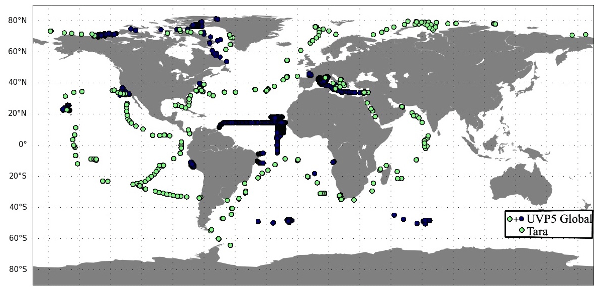
Figure 1 Location of the observations from the UVP5 database over the period 2009–2013. Green dots correspond to Tara expeditions and were included in the global UVP5 database.

2.1.1 Measurements of environmental and ecosystem variables (the drivers)

We use observations of environmental and ecosystem variables to determine the time and location of the observations that are co-located with the target variables. To represent the main physical and chemical drivers responsible for the concentration and variability of POC_S and POC_L we use measurements of ocean temperature, chlorophyll a, phosphate (PO₄), nitrates (NO₃) and mixed-layer depth (MLD). These variables were measured during Tara expeditions along with the particle size distributions and concentrations using UVP instruments on board these cruises. However, chlorophyll a, PO₄ and NO₃ were not measured systematically at each depth level. Thus, their averages over MLD are tested as possible drivers as well. To represent the biological drivers, we use information on PFTs.

2.1.2 The NEMO-PlankTOM12 global biogeochemical model

We used the output from the NEMO-PlankTOM12 coupled physical–biogeochemical model of the global ocean at daily and monthly time resolution. NEMO represents physical transport processes and is used in its v3.6-ORCA2 version, with a horizontal resolution of 2^∘ longitude and 0.3 to 1.5^∘ latitude and 31 vertical levels. It is forced by daily meteorological data from NCEP reanalysis (Kalnay et al., 1996) over the period 1948–2020, with output for 2009–2013 used here. This model version is identical to that used to estimate the ocean CO₂ sink in the Global Carbon Budget 2021 annual update (Friedlingstein et al., 2022).

PlankTOM12 represents ecosystem dynamics based on the representation of 12 PFTs: diatoms (DIA), mixed phytoplankton (MIX), coccolithophore (COC), picophytoplankton (PIC), phaeocystis (PHA), N₂ fixers (FIX), micro- or protozooplankton (PRO), pteropod (PTE), mesozooplankton (MES), gelatinous zooplankton (GEL) and bacteria (BAC). PlankTOM12 keeps track of the carbon biomass (µmol L⁻¹) of these PFTs over model depth levels resulting from environmental and ecosystem processes and their interactions (Le Quéré et al., 2016).

PlankTOM12 represents sinking processes through the explicit representation of two organic particle of different size, with small particles sinking at a constant speed of 3 m d⁻¹ and larger particles sinking at a variable speed between 3 and 150 m d⁻¹ depending on the ballast effect of their mineral content (Buitenhuis et al., 2013). In addition, a dissolved organic carbon component is transported via ocean currents. Particles are generated through mass flux from the PFTs resulting from mortality and egestion and from aggregation through differential sinking or turbulent coagulation and destroyed through grazing by zooplankton and remineralization by bacteria and through disaggregation from shear currents. Large PFTs contribute mostly to POC_L, while small PFTs contribute mostly to POC_S (Le Quéré et al., 2016; Fig. 2).

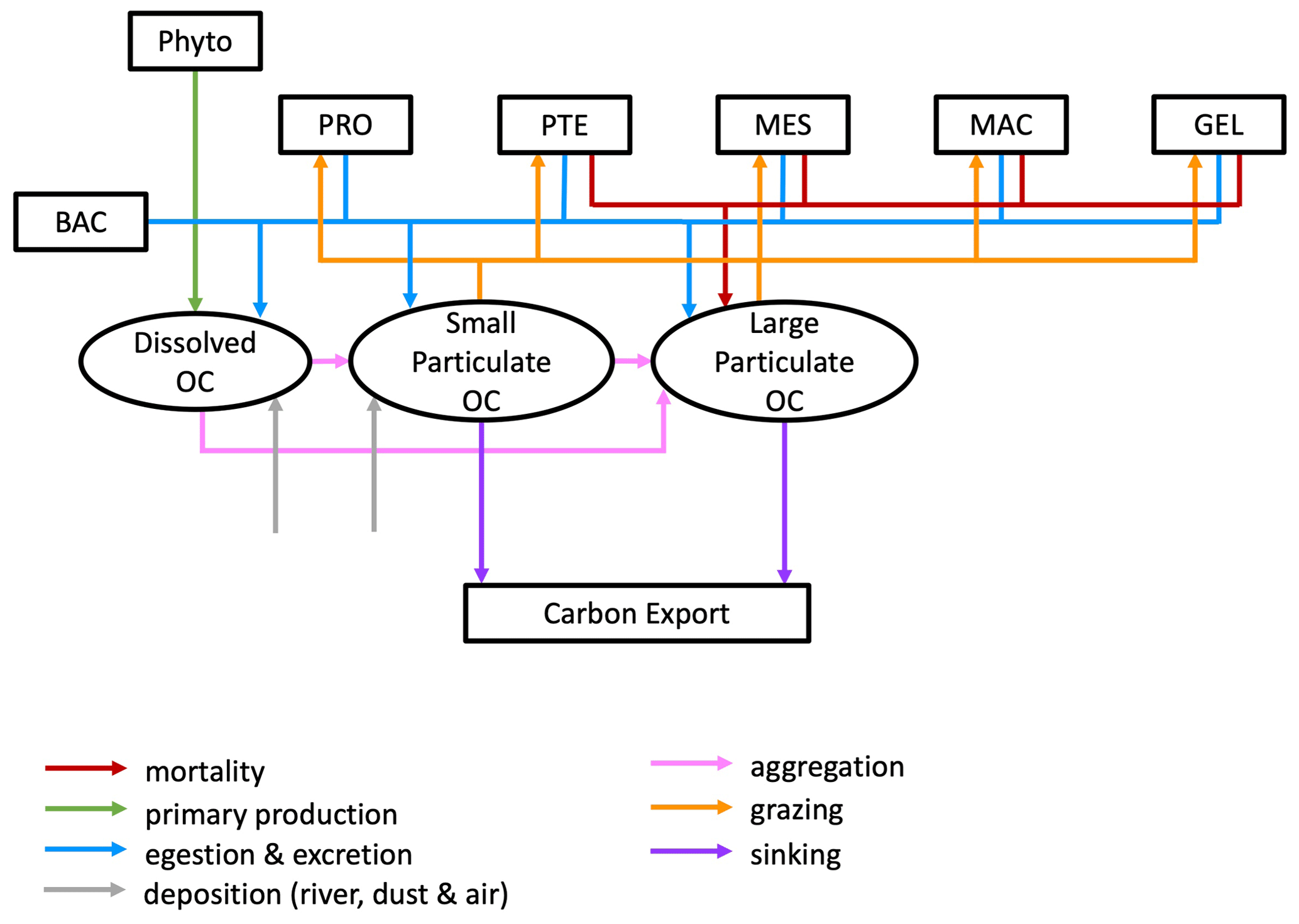
Figure 2 Schematic representation of the flow of matter in and out of the two particulate organic carbon (OC) components of the PlankTOM12 marine ecosystem model. The various boxes represent the following: Phyto – phytoplankton that includes diatoms (DIA), mixed phytoplankton (MIX), coccolithophore (COC), picophytoplankton (PIC), phaeocystis (PHA) and N₂ fixers (FIX); PRO – protozooplankton; PTE – pteropod; MES – mesozooplankton; MAC – macrozooplankton; GEL – gelatinous zooplankton; and BAC – bacteria.

The NEMO-PlankTOM12 model output was sampled at the time and location identified from the observations mentioned above to create a synthetic data set. The model grid-coordinate closest to the real geographical position was chosen. If several measurements were co-localized at the same grid coordinate and same time step (day for daily PlankTOM12 and month for monthly PlankTOM12 outputs), it is counted as one measurement. This model sampling produced 400 positions when using the daily or monthly PlankTOM12 outputs. All drivers and targets were taken from the model output at the corresponding coordinates up to 1400 m depth. These outputs served as the reference for validation and evaluation of the ML methods and for establishing the sets of the most important drivers.

2.2 Method

We tested two ML methods that are widely used in targets' reconstruction based on tabular data sets: the random forest regressor and the XGBoost (Extreme Gradient Boosting) regressor. The random forest (RF) regressor is an ensemble algorithm that contains a number of decision trees on various subsets of the given data set and takes as output the average of prediction from each tree estimator. RF can run several trees at the same time, allowing the use of a large number of input variables, and it is robust to overfitting (Biau, 2012). The XGBoost (XGB) regressor is an effective tree-based ensemble learning algorithm (Chen and Guestrin, 2016). It builds several models sequentially, where each new model attempts to correct errors from the previous one. XGBoost uses the gradient descent algorithm to minimize the loss function of the model. Using RF and XGBoost, we can estimate the driver importance to identify which driver has the greatest impact on the predictions. To check the driver importance, we use the drop_col_feat_imp Python function (https://gist.github.com/erykml/6854134220276b1a50862aa486a44192, last access: 18 May 2023). This method estimates how the accuracy of the ML output changes if one of the drivers is dropped off from a driver set (DS) based on the training data set.

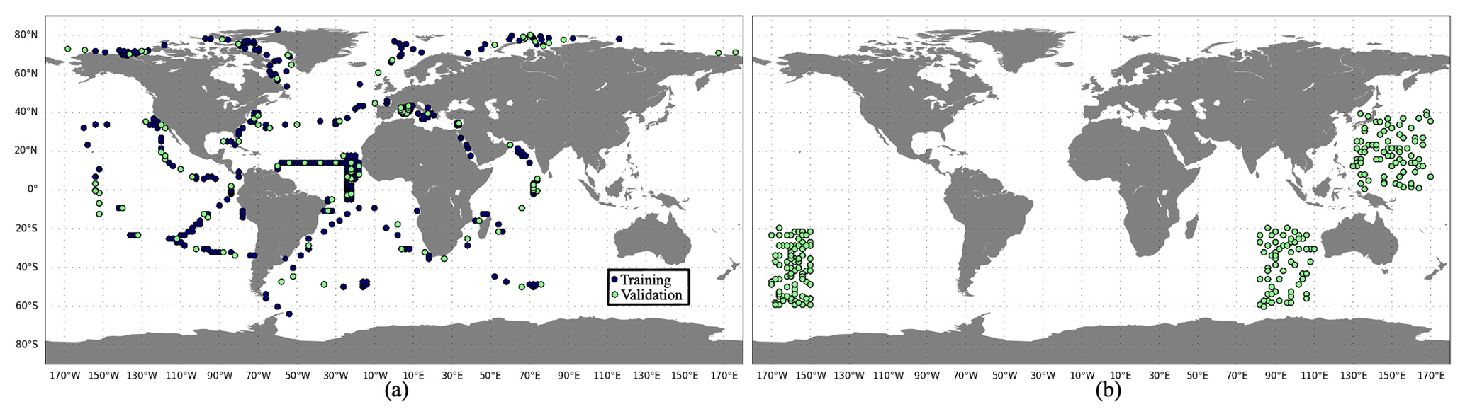
Figure 3 The spatial distribution of (a) training (blue) and validation (green) data sets and (b) the test data set, based on PlankTOM12 monthly outputs.

An effective ML algorithm requires sets of training, validation and test data. The training data build up the ML model. The model evaluates training data repeatedly to learn about the relationship between inputs (driver set) and known outputs (target set) and adjusts itself to better represent the target. The purpose of validation data is to evaluate the model during its training by introducing new unseen data. It allows us to evaluate how a developed model works on a new data set and to optimize hyperparameters. The test data evaluate the final accuracy of the ML model and confirm that the model works correctly on any unseen data. It is new data that did not participate in the training algorithm. The accuracy is worse for validation and test data compared to training data set. The difference in model performance on training and validation data can signal an overfitting, while this difference between validation and test data can demonstrate an effect of data mismatch. It is worth noting that RF does not necessarily need a validation data set as they perform internal validation. During the training algorithm, each tree is constructed from a random subset of original data. Usually it represents two-thirds of data, and one-third of data is used to estimate out-of-bag error to assess model performance. XGB uses a validation data set to evaluate the model during training and to prevent overfitting by applying an early stopping. In the present study, the available data were split into training and validation data sets (Fig. 3a). Validation data are not included in RF training; however we use them to test the performance of trained RF and tune hyperparameters afterwards. The test data are taken from the regions where there are no observations (Fig. 3b), i.e. 3 months for each year from the period 2009–2013, and six positions for each month were chosen randomly. This will allow us to identify the possible accuracy of reconstruction that can be reached in these regions when we apply a developed method to real observations. However, when POC_S and POC_L are reconstructed using only real-world observations, we will need to split all available data into training, validation and test data sets.

We use the RandomForestRegressor function from scikit-learn (https://scikit-learn.org/stable/modules/generated/sklearn.ensemble.RandomForestRegressor.html, last access: 18 May 2023) with its default parameters and min_sample_leaf equal to 20. To apply the XGBoost regressor, we use XGBRegressor from xgboost (https://xgboost.readthedocs.io/en/stable/python/python_intro.html, last access: 18 May 2023). Parameters were set as follows: n_estimators = 2000, max_depth = 7, eta = 0.01, subsample = 0.7, colsample_bytree = 0.8, gamma = 0.01 for POC_L and gamma = 0.3 for POC_S, and early_stopping_rounds  = 10.

We tested 27 driver sets (DSs) that are summarized in Table 1. For each DS, we identify the most important drivers that influenced the reconstruction of small (POC_S) and large (POC_L) particulate organic carbon concentration. The drivers include geographic variables (depth, sin(latitude), cos(longitude)), physical variables (incident light, MLD, co-located temperature), chemical variables (PO₄ and NO₃, including co-located values and averages over the MLD) and biological variables (chlorophyll a, 12 PFTs listed above: DIA, MIX, COC, PIC, PHA, FIX, PRO, PTE, MES, GEL and BAC, including co-located values and averages over the MLD).

Table 1 Compounds of driver's sets: dark grey cells correspond to the drivers present in the driver set. “vp” – vertical profile, “mean” – average over MLD, “back” – values from previous month.

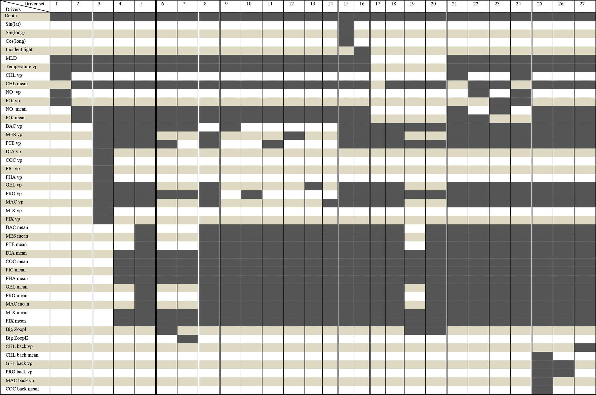
The driver sets can be split into nine thematic groups which together test the role of PFTs and sub-classes within, the role of surface versus depth profiles for some variables and the role of information from the previous month:

• i.

  No PFTs (short name (sh.n.) “No PFT”). Driver sets 1 and 2 do not include any PFTs and focus on the influence of temperature, MLD, chlorophyll a, NO₃ and PO₄ on POC_S and POC_L reconstruction.

• ii.

  Introduction of PFTs (sh.n. “PFT introduction”). DSs 3, 4 and 5 are dedicated to the investigation of the introduction of PFTs in the reconstruction. In DS 3 we introduced 12 PFTs vertical profiles, even though this information will be challenging to reproduce with observations due to a lack of data. Nevertheless, it is important to test the capacity of ML if all 12 PFTs were available over the depth. DS 4 includes the vertical profiles of six heterotrophs (zooplankton and bacteria) because they contribute to influencing the vertical distribution of POC_S and POC_L and six phytoplankton averaged over MLD because they are responsible for primary production. In DS 5 we added averages over MLD of the six heterotrophs that were not included in DS 4.

• iii.

  Big zooplankton (sh.n. “Zooplankton combined”). In DSs 6 and 7 we tested the influence of big zooplankton summed into one variable to account for their combined effect rather than the distinctions among PFTs. The big zooplankton is represented by the sum of mesozooplankton, gelatinous zooplankton and macrozooplankton in DS 6, with the addition of pteropod in DS 7.

• iv.

  Exclusion of bacteria (sh.n. “No vertical BAC”). DS 8 does not have a bacteria (BAC) vertical profile compared to set 5.

• v.

  Individual zooplankton types (sh.n. “Individual PFT”). DSs 9, 10, 11, 12, 13 and 14 test the influence of individual types of heterotrophs, bacteria (BAC), microzooplankton (PRO), pteropod (PTE), mesozooplankton (MES), gelatinous zooplankton (GEL) and microzooplankton (MAC), respectively.

• vi.

  Geographical position and seasons (sh.n. “Lat-Long” and “Incident light”). DS 15 is based on DS 5 (which showed the most promising results) and includes geographical coordinates as additional drivers in the form of sin(lat), sin(long) and cos(long). DS 16 includes in addition to the DS 5 the role of incident light.

• vii.

  Use of only PFTs and chlorophyll a (sh.n. “PFT only + CHL”). DS 17 is only based on the 12 PFTs, while DS 18 is formed from DS 17 and information on chlorophyll a averaged over the MLD. DSs 19 and 20 are based on DS 6. To form the DS 19, we exclude temperature, NO₃ and PO₄ from the list of drivers in DS 6. DS 20 is an extended version of DS 19 with all 12 PFTs' concentration averaged over the MLD.

• viii.

  Chlorophyll a and chemical variables (sh.n. “Biochemical variables”). DSs 21, 22, 23 and 24 are based on DS 5 and test the individual influence of chlorophyll a (DS 21), NO₃ (DS 22), and PO₄ (DS 23) vertical profiles and their ensemble (DS 24).

• ix.

  Previous time step (sh.n. “Month − 1”). DSs, 25, 26 and 27 investigate the role of chlorophyll a (DS 27) and some zooplankton from the previous time step: gelatinous zooplankton and microzooplankton (DS26) as well as gelatinous zooplankton and micro- and macrozooplankton, averaged over MLD chlorophyll a and coccolithophore (DS25).

The evaluation of the method is based on the mean correlation coefficient, total root mean square errors (RMSEs) and total absolute bias between the ML outputs and PlankTOM12 POC_S and POC_L components. Moreover, we provide the global maps of correlation coefficient and RMSE to vertical profiles of POC_S and POC_L at each grid point. Global maps help to identify zones where the large errors can be hidden in the mean diagnostics due to the error compensation.

3 Results

3.1 Data analysis

In this study we test the capacity to reconstruct particulate organic carbon from sparse observations by using ML and a synthetic data set based on the PlankTOM12 model output. We compare observations and the output of the ocean model to provide a minimum of validation for the model data and to help explain differences in ML results when applied to real observations in the future.

Figure 4 shows the vertical profile of small (POC_S) (Fig. 4a) and large (POC_L) particulate organic carbon (Fig. 4b) based on the median from observations (green) and from daily PlankTOM12 model output (blue). Shading corresponds to values between 0.25 and 0.75 percentiles.

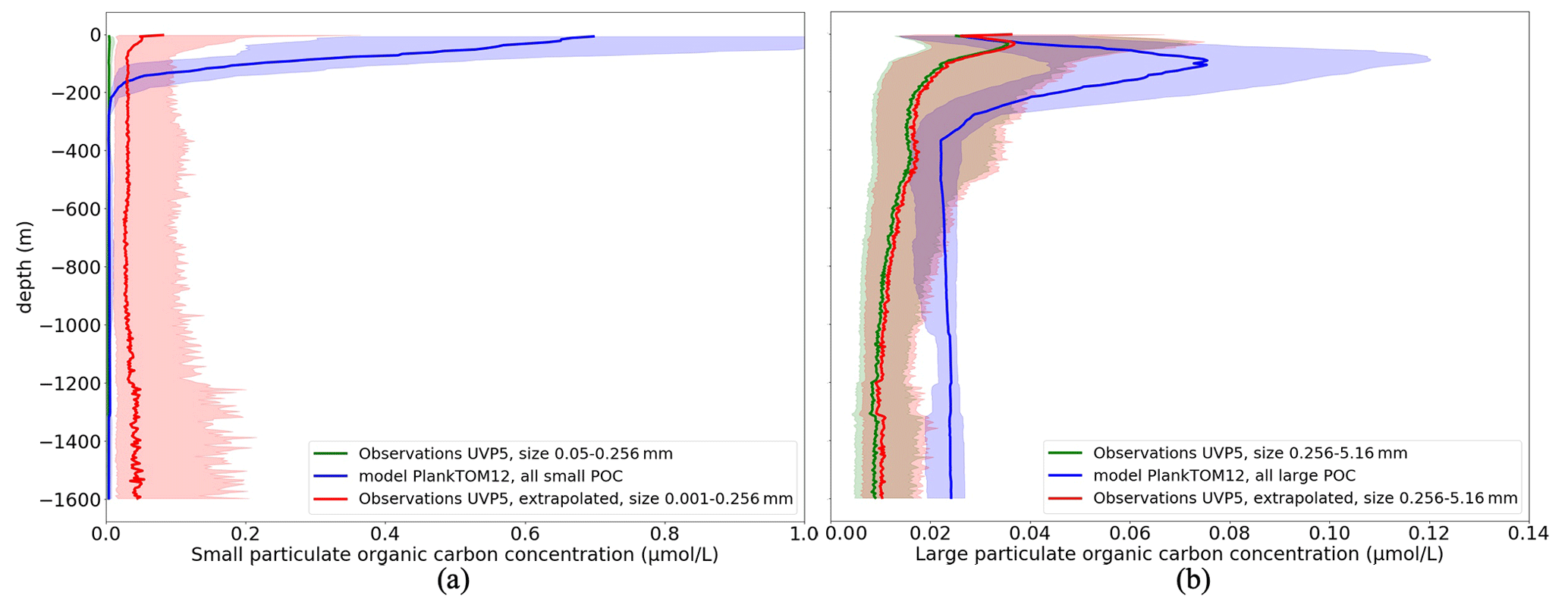
Figure 4 Comparison of the vertical distribution of particulate organic carbon concentrations (µmol L⁻¹) from UVP5 measurements (green), PlankTOM12 daily model (blue) and extrapolated UVP5 measurements (red): (a) small particulate organic carbon concentrations and (b) large particulate organic carbon concentrations. The median is shown in dark, and the shading corresponds to values between the 0.25 and 0.75 percentiles. The size of the particles does not correspond completely between the observations and the model; for POC_L the UVP particle range is chosen as 0.256–5.16 mm, which corresponds approximately to the POC_L in the model.

PlankTOM12 overestimates POC_S up to 3 µmol L⁻¹ in the first 200 m (Fig. 4a, green and blue curves). UVP5 does not capture all small particles, which is why we extrapolated the size range of UVP measurements (red curve; see details in Sect. 2.1.1). The extrapolated measurements show an increase in POC_S in the first 100 m; however this increase still results in the lower concentration compared with PlankTOM12. These results indicate that PlankTOM12 overestimates the concentration of small particulate organic carbon. PlankTOM12 also overestimates POC_L by up to 0.08 µmol L⁻¹ in the first 200 m and does not catch the increase in POC_L between 300 and 500 m. Observations show an increase in POC_L concentration in the first 50 m, while PlankTOM12 reproduces it at a lower level, at 100 m. The RMSE between modelled and observed POC_S is 0.33 µmol L⁻¹, with a correlation coefficient equal to 0.083. The RMSE is 0.23 µmol L⁻¹, with a correlation coefficient of 0.061 for POC_L. The exclusion of isolated large values of POC_L (> 2 µmol L⁻¹) from the observation data set reduces the RMSE of POC_L to 0.062 µmol L⁻¹, with a correlation of 0.18. We believe that these differences result from differences in space and time resolution of observations and ocean model outputs. In situ measurements are obtained at a particular time of the day and a particular latitude–longitude position, while the model provides estimations over the day (or month) and on the model grid (2^∘ longitude and mean 1.1^∘ latitude resolution).

We concluded that observed and modelled POC_S and POC_L have a common tendency in their vertical distributions. However, among other things, differences in amplitudes may affect our findings in this work when we develop a ML method based on observations only.

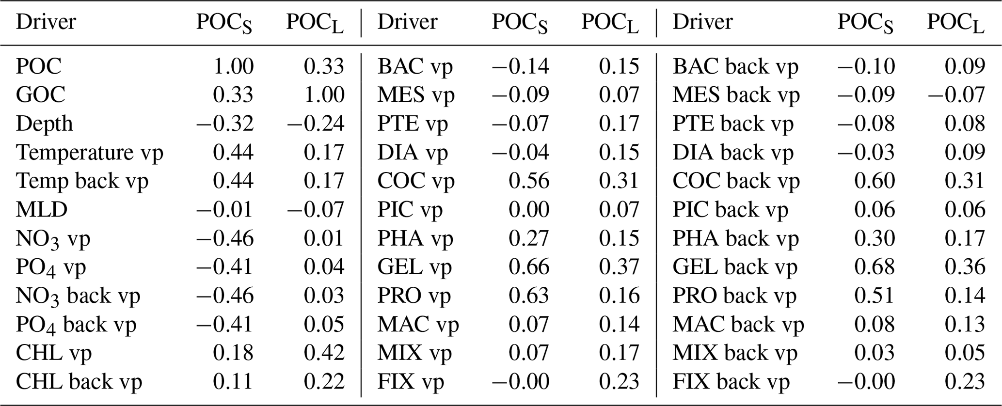
Due to the constraints in data availability, we further use monthly PlankTOM12. Before developing a ML method, we investigate the interactions between targets and drivers in the model. Table 2 shows the correlation coefficients between the POC_S and POC_L and corresponding drivers that can influence POC_S and POC_L variability. Correlation between drivers could also provide valuable information to minimize the number of drivers, but they are not shown here where the focus is on discovering the effect of a large set of drivers on POC distribution and because driver correlations could also result from the physics as well as from the model construction. POC_S correlates with gelatinous zooplankton (GEL, r = 0.66), microzooplankton (PRO, r = 0.63) and coccolithophore (COC, r = 0.56), as well as with their values from the previous time step (GEL, r = 0.67; PRO, r = 0.51; COC, r = 0.59). Coccolithophore is one of the most abundant phytoplankton types in this version of the PlankTOM model (similar to Wright et al., 2021). The growth of phytoplankton transfers dissolved inorganic carbon into dissolved organic carbon, which further aggregates into POC_S and POC_L. Also, POC_S is generated from microzooplankton egestion and excretion (Fig. 2). In addition to the above-mentioned PFTs, POC_S shows a correlation 0.44 with the temperature vertical profile at both the considered time step and at the previous time step. POC_S has negative correlations with NO₃ (r = −0.46) and PO₄ (r = −0.41).

POC_L does not show a high correlation with any of the proposed drivers individually and is therefore most likely the result of multiple processes and/or multiple drivers, including for its production and destruction. The ML approach should be able to identify combinations of drivers beyond straight correlations that are investigated directly here. POC_L has the highest correlation with chlorophyll a (r = 0.42) and gelatinous zooplankton at the considered time step (r = 0.37) and at the previous time step (r = 0.36). Gelatinous zooplankton contributes to POC_L formation through egestion and excretion mainly from mucus (Fig. 2). As explained in Wright et al. (2021), mucus forms a large low-density mass through aggregation with other particles. It can explain a correlation of gelatinous zooplankton with POC_L in PlankTOM12.

Table 2 Correlation coefficient between small (POC_S) and large (POC_L) particulate organic carbon concentration and possible drivers. Estimation is based on monthly PlankTOM12 output at the position of real-world observations from Fig. 1. “vp” – vertical profile, “mean” – average over MLD and “back” – values from previous month.

3.2 Development of the machine learning method

We tested 27 sets of drivers (Table 1) and two ML methods, random forest (RF) and XGBoost regression (XGB).

Figure 5 shows the statistics of POC_S reconstruction using RF and XGB. XGB (orange) generally outperforms RF (blue). The statistics are slightly worse for the validation and test data sets, as expected. For reconstructions using XGB, the RMSE and absolute bias are about 0.05 and 0.03 µmol L⁻¹ on the training data set and vary around 0.1 and 0.05 µmol L⁻¹, on the validation and test data, respectively. Correlation coefficients (Fig. 5g, h, i) have high values for all data sets, showing that the vertical profiles of POC_S have the correct shape. These results show that the available spatial and temporal coverage of in situ observations can be sufficient to reconstruct POC_S with an appropriate accuracy over the global ocean. The analysis of global maps (shown below) will help to identify areas with low accuracy and their differences with training regions.

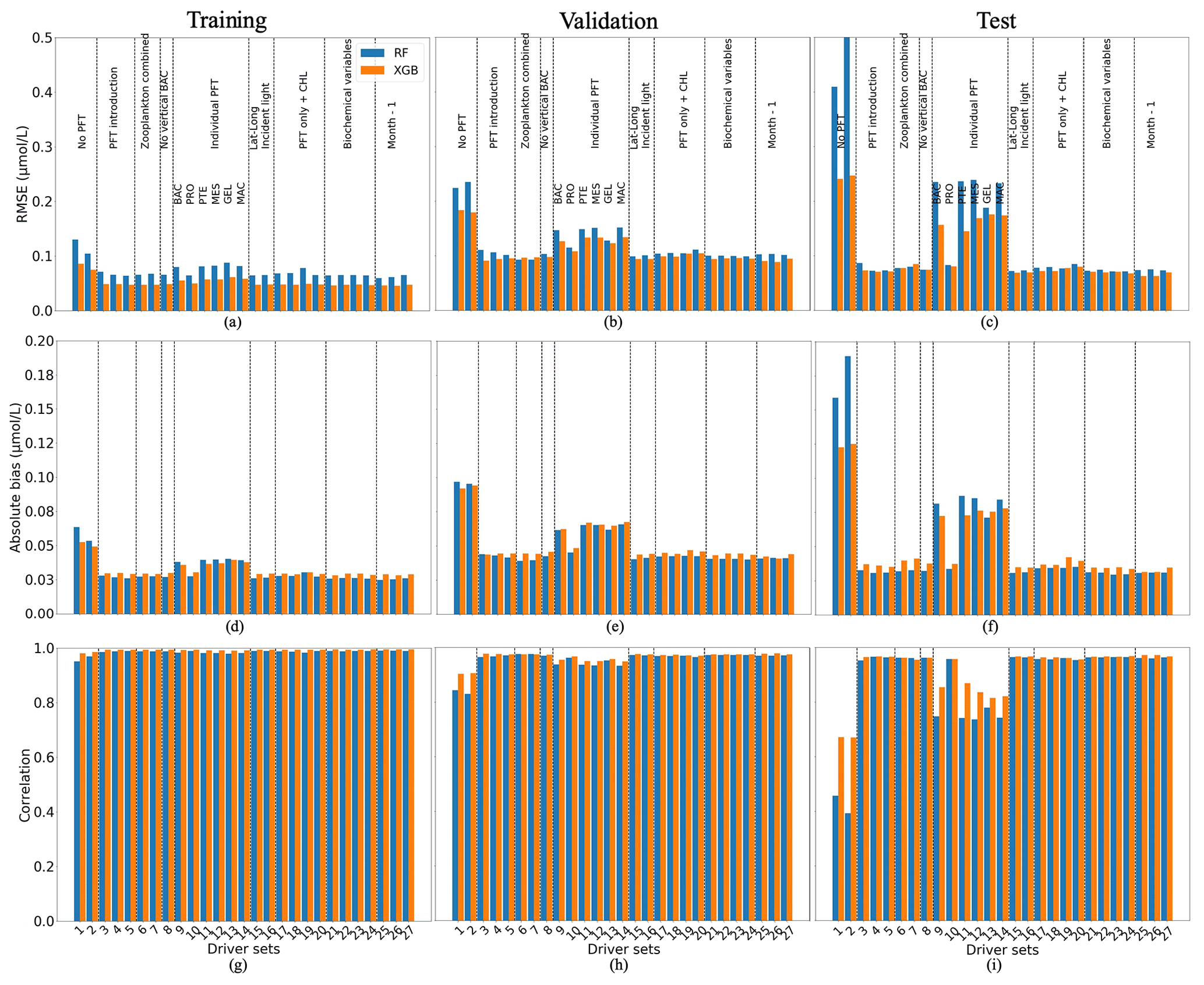
Figure 5 Comparison of the performance of the random forest (RF) and XGBoost methods and their fit to data for small (POC_S) particulate organic carbon concentration: (a, b, c) RMSE (in µmol L⁻¹), (d, e, f) absolute bias (in µmol L⁻¹) and (g, h, i) correlation coefficient. (a, d, g) The training data set, (b, e, h) the validation data set and (e, f, i) the test data set. Results compare data from the original (sampled) PlankTOM12 model output and POC_S reconstructed using RF (blue) and XGB (orange). The low RMSE and absolute biases indicate better performance of the ML method.

The worst results (highest RMSE, highest absolute bias and lowest correlation) are produced when there are no PFTs in the driver set (DS1 and DS2; Fig. 5): for XGBoost, RMSEs are 0.24 µmol L⁻¹, and absolute biases are equal to 0.12 µmol L⁻¹ with a correlation coefficient of 0.67 on the test data sets. Poor results are also obtained for DSs 9, 11, 12, 13 and 14: these five driver sets do not have any information on microzooplankton (PRO) and show high RMSEs and absolute biases, around 0.16 and 0.074 µmol L⁻¹, with low correlation, 0.83, compared with other driver sets which include PRO. These results indicate that microzooplankton plays an important role in POC_S variability in the PlankTOM12 model.

Figure 6 shows the statistics of POC_L reconstruction using RF and XGB. XGBoost again slightly outperforms RF for most driver sets. Results for driver sets with PFTs show lower RMSEs and absolute biases and higher correlation coefficients. Except for the effect of PFTs on the POC_L reconstruction, we did not observe a clear influence of one driver or group of drivers. Using XGBoost, the reconstruction of POC_L shows the RMSE in DS1 is high at 0.03 µmol L⁻¹, while it is in the range of 0.021–0.026 µmol L⁻¹ in DS3–DS27, with absolute bias in DS1 of 0.02 and 0.015–0.018 µmol L⁻¹ for DS3–DS27 based on test data (Fig. 6c, f). Likewise, there is a correlation coefficient of 0.56 for DS1 and between 0.7 and 0.77 for DS3-DS27 based on the training data set (Fig. 6g).

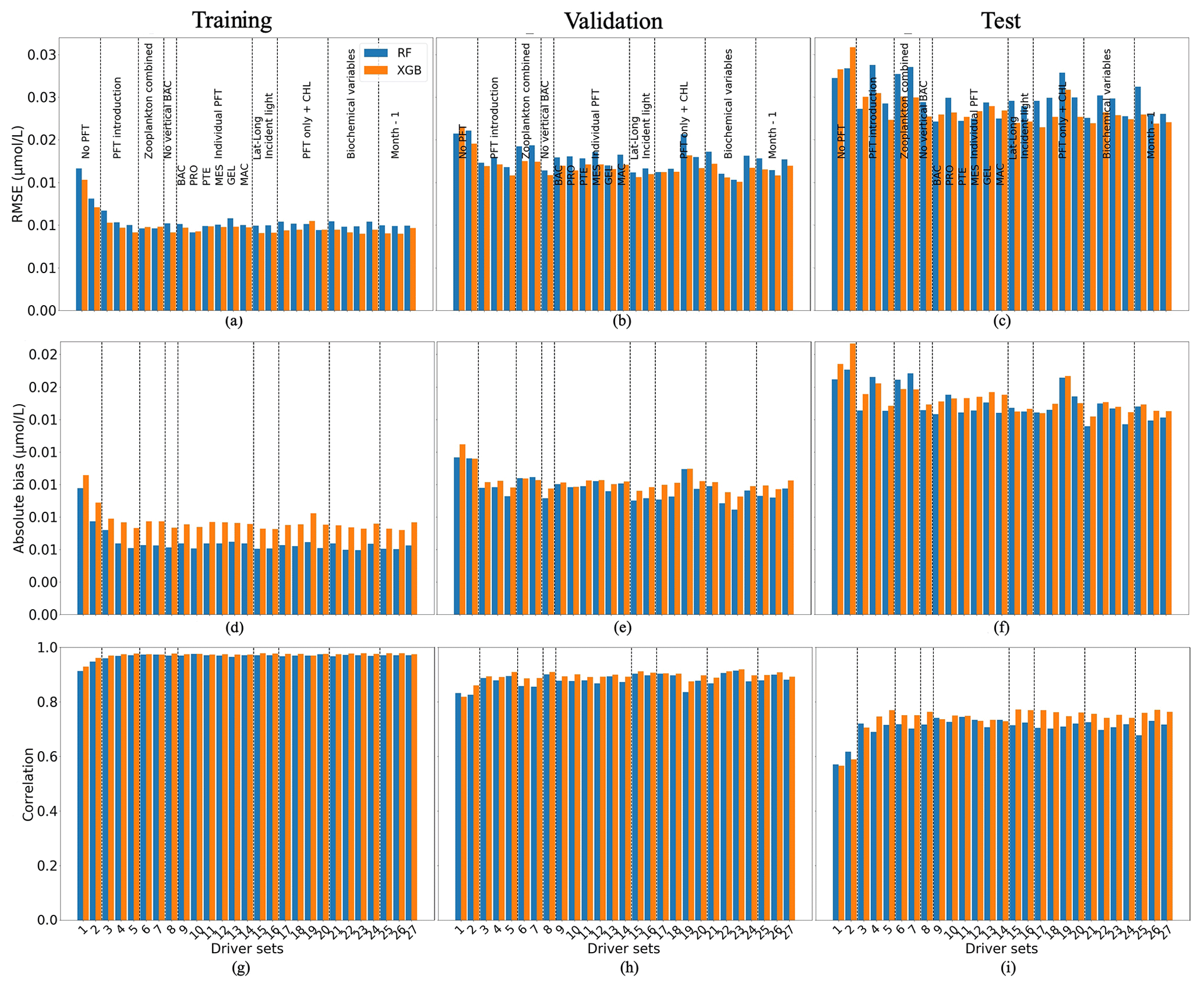
Figure 6 Comparison of the performance of the random forest (RF) and XGBoost methods and their fit to data for large (POC_L) particulate organic carbon concentration; (a, b, c) RMSE (in µmol L⁻¹), (d, e, f) absolute bias (in µmol L⁻¹) and (g, h, i) correlation coefficient. (a, d, g) The training data set, (b, e, h) the validation data set and (e, f, i) the test data set. Results compare data from the original (sampled) PlankTOM12 model output and POC_L reconstructed using RF (blue) and XGB (orange). The low RMSE and absolute biases indicate better performance of the ML method.

We estimated the ranking of importance for each driver averaged over 27 driver sets (Table 1) for RF and XGB (Fig. 7). Both RF and XGB show that microzooplankton (PRO), depth level, temperature, NO₃ and PO₄ play a dominant role in reconstruction of POC_S. The absence of gelatinous zooplankton (GEL) can slightly improve the reconstruction. Also, latitude and longitude do not affect POC_S reconstruction. The depth level, temperature, MLD, microzooplankton (PRO) and phaeocystis (PHA), PO₄, and chlorophyll a averaged over MLD play a dominant role in POC_L reconstruction.

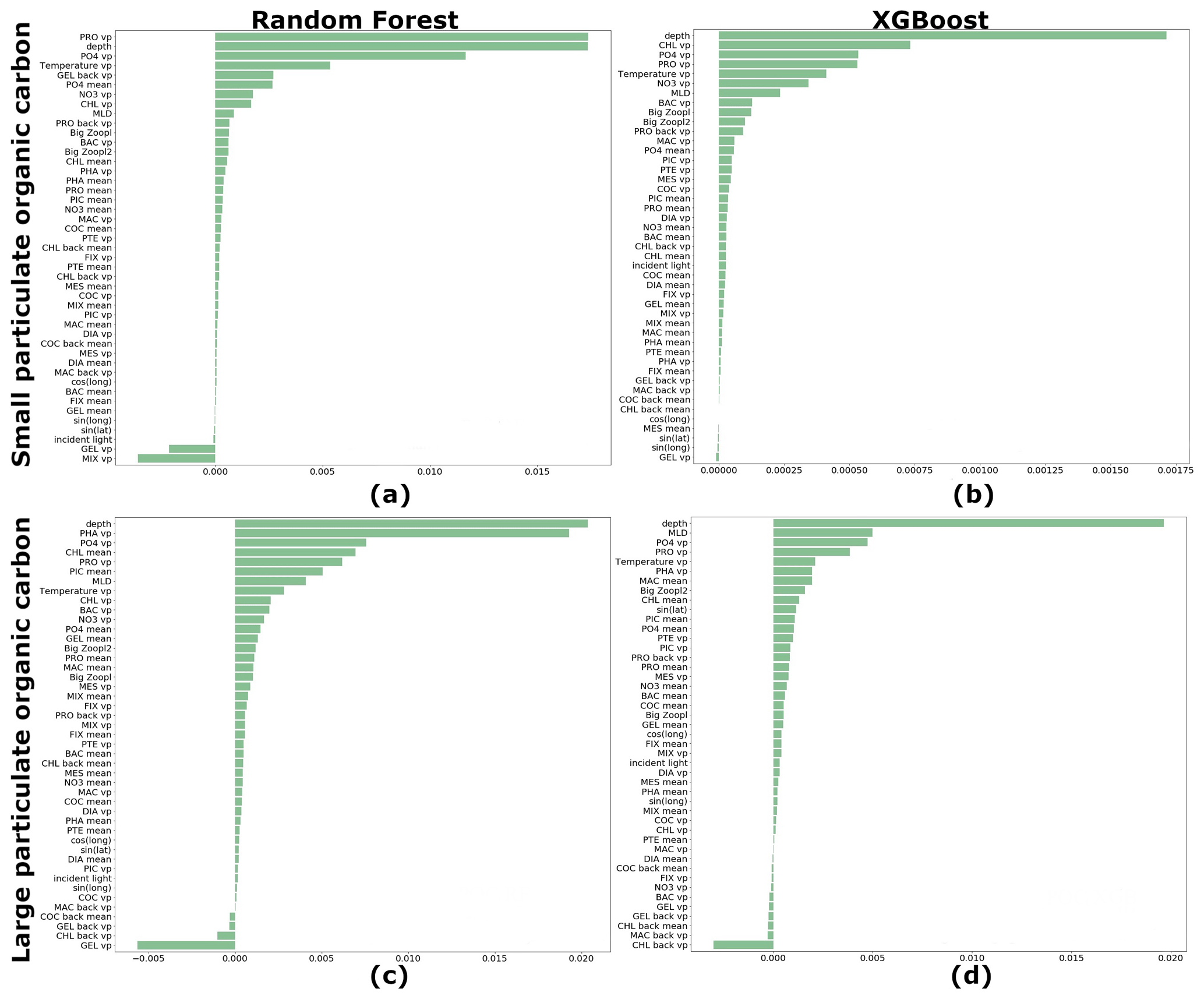
Figure 7 Ranking of importance for each driver averaged over 27 driver sets: (a) random forest (RF) for reconstruction of small (POC_S) particulate organic carbon concentration, (b) XGBoost (XGB) for reconstruction of POC_S, (c) RF for reconstruction of large (POC_L) particulate organic carbon concentration and (d) XGB for reconstruction of POC_L. “vp” – vertical profile, “mean” – average over MLD and “back” – values from previous month.

The sinus of latitude is in the top 10 drivers that most affect POC_L using the XGBoost method: the POC_L distribution has a lot of meridional variability that results in the sinus of latitude being in the top 10 drivers. As for POC_S, gelatinous zooplankton (GEL) shows a negative rank of driver importance, and its removal from the list of drivers can improve the statistics of reconstruction. Also, chlorophyll a concentration from the previous month shows a similar effect on POC_L (Fig. 7c, d).

It is worth noting that any driver that shows negative importance in the reconstruction only has a small influence on the accuracy (Figs. 5 and 6). Thus, its removal does not improve the reconstruction significantly.

Based on Figs. 5, 6 and 7 we have chosen 10 driver sets with low RMSEs and absolute biases and high correlation coefficients (based on test data set) for POC_S and POC_L to provide global maps of these statistics and to see their regional distributions. DSs 5, 15, 16, 21, 22, 23, 24, 25, 26 and 27 were chosen for further investigation of POC_S reconstruction and DSs 5, 8, 15, 16, 17, 21, 23, 25, 26 and 27 for POC_L reconstruction. Common for POC_S and POC_L driver sets 5, 15, 16, 21, 23, 25, 26 and 27 is that they include all PFTs and their average over MLD, geographical positions and incident light, as well as chlorophyll a, PO₄ and gelatinous zooplankton and microzooplankton from the previous time step (Table 1). Also, we found that POC_S reconstructions rest on biochemical conditions (DSs 21 and 24), while POC_L reconstruction mostly depends on the composition of the PFTs in the driver set (DSs 8 and 17). Additionally, we keep DS1 to demonstrate a global effect of PFTs on reconstruction.

3.3 POC_S and POC_L vertical profile reconstruction over the global ocean

In the previous section we showed that XGBoost provides the best results for the reconstructions of POC_S and POC_L. Further we use this ML method. Here we will discuss the regional results of DS1 without PFTs and the 10 best driver sets chosen for each target separately.

Figure 8 shows POC_S and POC_L concentration averaged over the depth and period 2009–2013 for PlankTOM12 (Fig. 8a, b), XGBoost reconstruction based on DS1 (Fig. 8c, d) and XGBoost reconstruction based on DS25 (Fig. 8e, f). XGBoost captures the spatial patterns well: the high concentration of POC_S in the equatorial eastern Pacific and its low concentration at high latitudes, as well as the high concentration of POC_L in the equatorial eastern Pacific and in the north of the Indian Ocean and its low concentration in the subtropical North and South Atlantic and in the subtropical North Pacific. The presence of PFTs in driver sets (Fig. 8e, f) improves the reconstruction: the spatial patterns and POC amplitude are visually close to ones from PlankTOM12 (Fig. 8a, b). The high concentration of POC_S in the equatorial eastern Pacific is represented better using DS25 compared with DS1, where the concentration in the latitude band 0–20^∘ S along the Peru is overestimated. Also, small decreases of POC_S in the subtropical North and South Atlantic are captured better when we use DS25. Similar for POC_S, the high concentration in the equatorial eastern Pacific is represented better using DS25 compared with DS1, where the concentration misses the small decrease between 20 and 0^∘ N. Also, small decreases of POC_L in the subtropical North and South Atlantic as well as in the subtropical North Pacific are pronounced better with DS25.

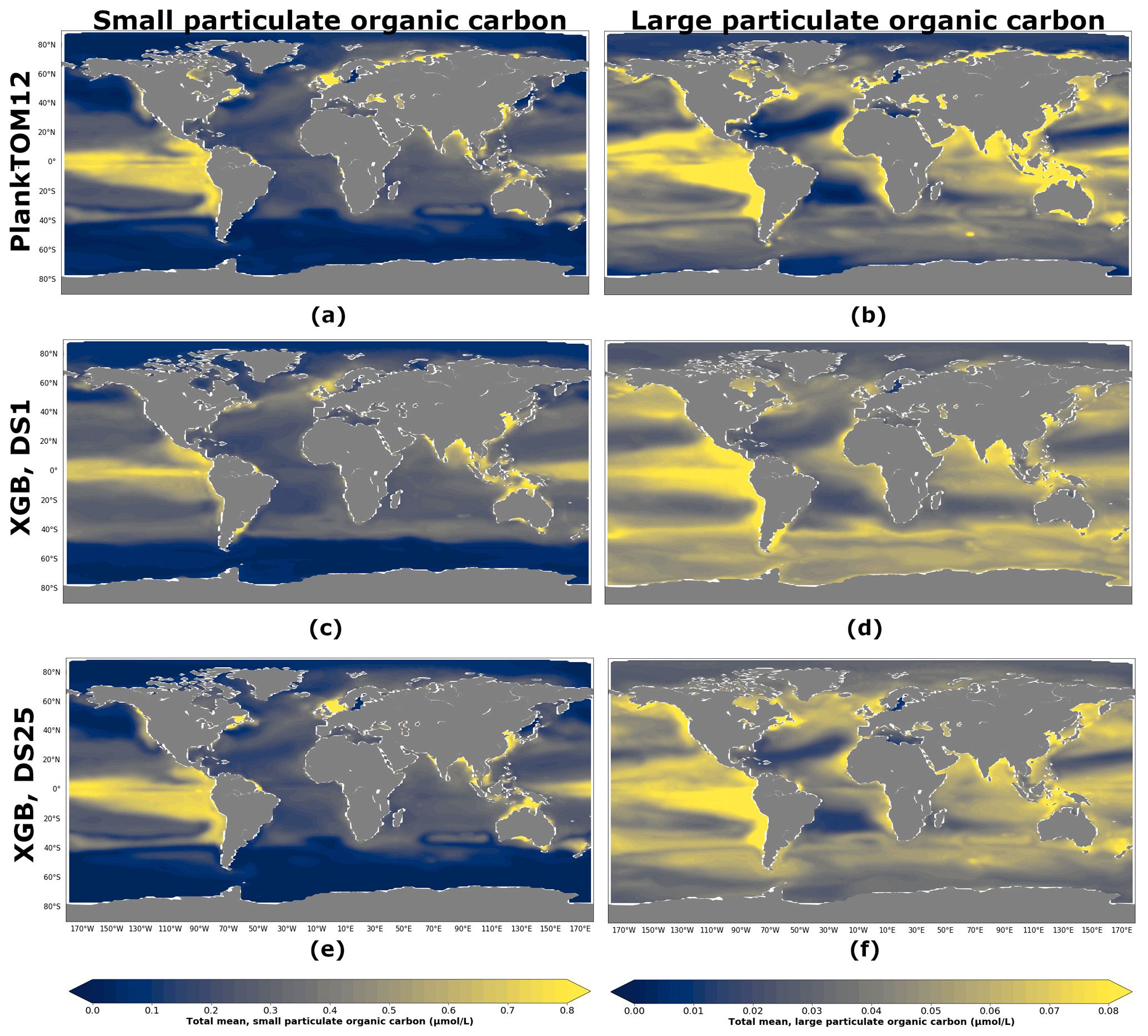
Figure 8 Total small (POC_S) and large (POC_L) particulate organic carbon concentration averaged over the depth and period 2009–2013: (a) PlankTOM12 POC_S, (b) PlankTOM12 POC_L, (c) reconstruction of POC_S based on DS1 (NoPFT) using XGBoost, (d) reconstruction of POC_L based on DS1 using XGBoost, (e) reconstruction of POC_S based on DS25 (vertical profiles of zooplankton as well as zooplankton and phytoplankton averaged over MLD) using XGBoost, (f) reconstruction of POC_L based on DS25 using XGBoost.

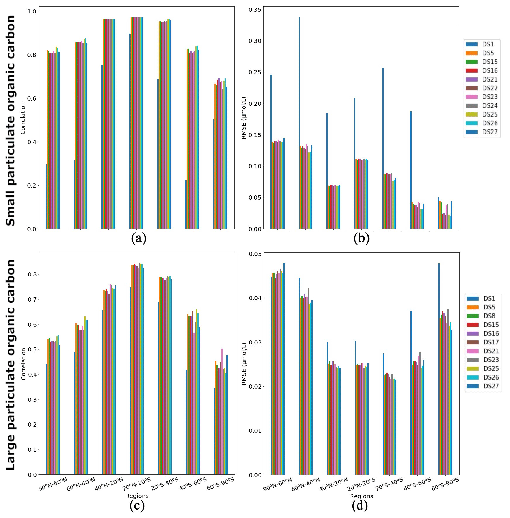
Figure 9 Correlations and RMSE averaged over latitude zones between PlankTOM12 and XGBoost reconstruction over the global ocean for 2009–2013: (a, c) correlation coefficient and (b, d) RMSE (in µmol L⁻¹). (a, b) Small particulate organic carbon (POC_S) and (c, d) large particulate organic carbon (POC_L).

Figure 9 shows regional correlation coefficients and RMSEs between PlankTOM12 and XGBoost reconstruction over the global ocean for 2009–2013. We averaged correlation coefficient and RMSEs over seven latitude zones: 90–60^∘ N, 60–40^∘ N, 40–20^∘ N, 20^∘ N–20^∘ S, 20–40^∘ S, 40–60^∘ S and 60–90^∘ S. In POC_S reconstruction, the DS1 shows the lowest correlation across latitude bands (between 0.22 and 0.9) and highest RMSEs (0.05–0.34 µmol L⁻¹; Fig. 9a, b). DSs 25 and 26 show the highest correlations in the range of 0.68 (in region 60–90^∘ S) and 0.97 (in region 20^∘ N–20^∘ S) and the lowest RMSEs in the range of 0.021 (in region 60–90^∘ S) and 0.14 µmol L⁻¹ (in region 90–60^∘ N). DS25 contains information on the previous month's distribution for micro- and macrozooplankton and gelatinous zooplankton vertical profiles as well as coccolithophores and chlorophyll a averaged over the MLD. DS26 is like DS25, but the drivers which bring information from the previous month are microzooplankton and gelatinous zooplankton vertical profiles.

A total of 10 driver sets (excluding DS1) show their highest RMSEs in POC_S reconstruction in the region 90–60^∘ N, with values up to 0.14 µmol L⁻¹ in DS27 (Fig. 9b). Figure 10 shows maps of RMSEs (a, b) and correlation coefficients (c, d) between PlankTOM12 and reconstructed small particulate organic carbon (POC_S) by XGBoost using driver sets 1 (a, c) and 25 (b, d). The region 90–60^∘ N shows improvement in RMSEs and absolute biases in DS25 compared with DS1, with RMSEs decreasing from 0.2 to 0.03 µmol L⁻¹ in the Norwegian Sea, Baffin Bay and the Arctic Ocean. However, errors stay high in the coastal regions, Northwest Passage and Hudson Bay, which contribute to the high total RMSEs in this region. Results are similar for the region 60–40^∘ N, where correlation coefficients increased from 0.3 to 0.87 on average over these zones (Fig. 10c, d). The tropical region 20^∘ N–20^∘ S shows correlation coefficients up to 0.97 for all driver sets except DS1. However, RMSEs are high in the tropical region, about 0.11 µmol L⁻¹ on average (Fig. 9b), with RMSEs values of 0.2 µmol L⁻¹ in the tropical eastern Pacific and Bay of Bengal in DS25 (Fig. 10b). The high RMSEs in the tropical eastern Pacific can indicate insufficient data in a region of high interannual variability to correctly reconstruct POC_S distribution. The region of the Southern Ocean (> 60^∘ S) shows the lowest correlation coefficients (in the range of 0.64–0.69) and RMSEs (in the range 0.023–0.044 µmol L⁻¹) for POC_S (Fig. 9a, b). The inclusion of PFTs in the driver set significantly improves the RMSE in the region around 40^∘ S for small (POC_S) particulate organic carbon. The statistics are improved by about 75 % in the region 40–60^∘ S with RMSE decreasing from 0.18 (DS1) to 0.03 (DS25) and the correlation coefficient increasing from 0.22 (DS1) to 0.84 (DS25), on average (Fig. 9a, b; Fig. 10). The improvements in the Southern region are related to the role of zooplankton in the carbon flux in this area (Le Quéré et al., 2016; Wright et al., 2021).

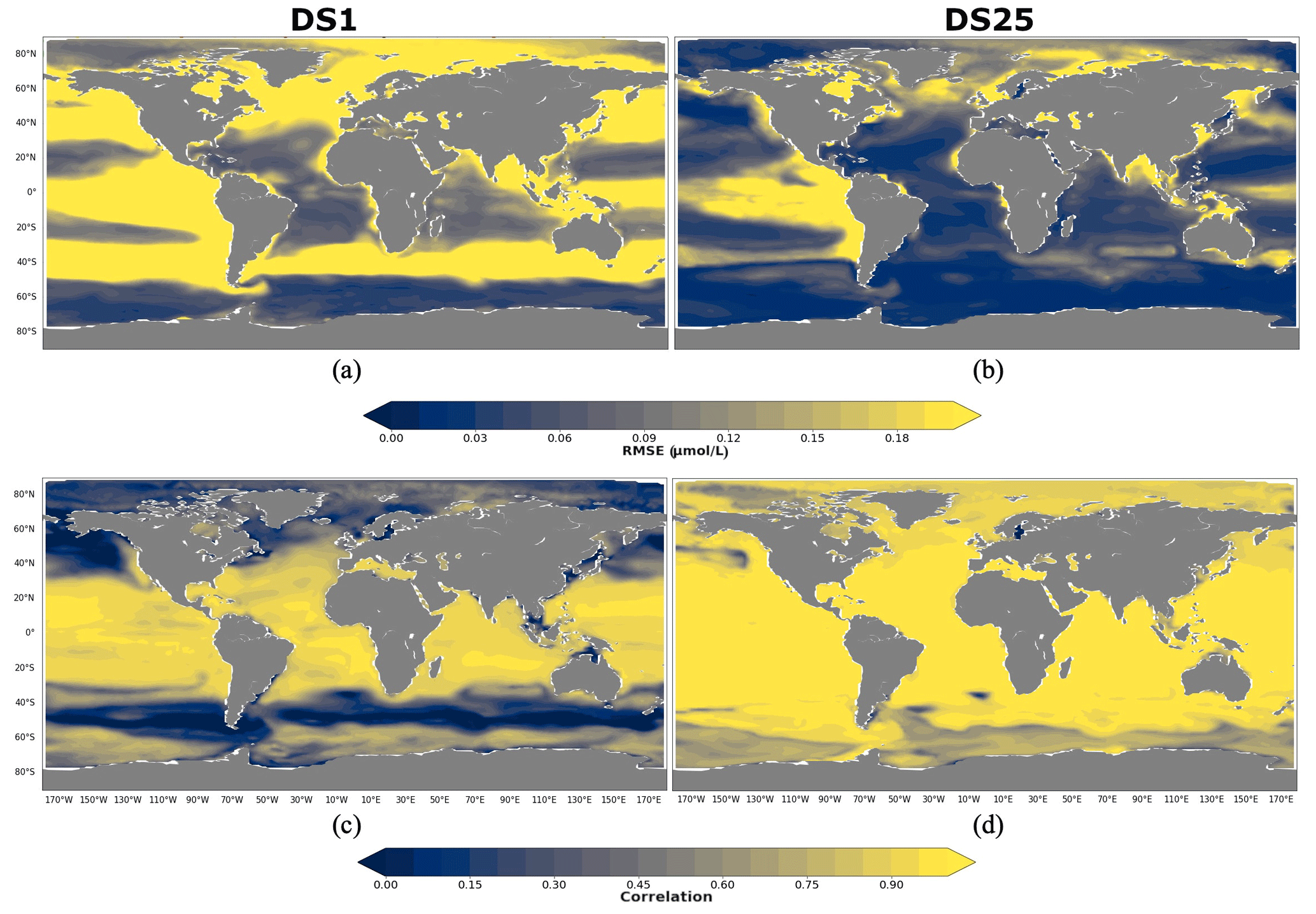
Figure 10 RMSE and correlation between monthly PlankTOM12 and results of POC_S reconstruction using XGBoost over the period 2009–2013 for POC_S. (a, b) RMSEs and (c, d) correlation coefficients. (a, c) Reconstruction based on DS1 (NoPFT) and (b, d) reconstruction based on DS25 (vertical profiles of zooplankton as well as zooplankton and phytoplankton averaged over MLD).

In POC_L reconstruction, DS1 also shows the lowest correlation coefficients (0.35–0.75) and the highest RMSEs (0.027–0.47 µmol L⁻¹) (Fig. 9c, d). DS25 shows the best results on average, with the correlation coefficient varying between 0.43 (in the region 60–90^∘ S) and 0.84 (in the region 20^∘ N–20^∘ S) and RMSE varying between 0.021 (in the region 20–40^∘ S) and 0.046 (in the region 90–60^∘ N) µmol L⁻¹. POC_L are reconstructed better in subtropical and tropical regions compared to high-latitude zones (Fig. 9c, d).

As for POC_S, 10 driver sets (excluding DS1) show their highest RMSEs in POC_L reconstruction in the region 90–60^∘ N, with values up to 0.05 µmol L⁻¹ in DS27 (Fig. 9d). Figure 11 shows maps of RMSEs (a, b) and correlation coefficients (c, d) between PlankTOM12 and reconstructed large particulate organic carbon (POC_L) by XGBoost using driver sets 1 (a, c) and 25 (b, d). In contrast to POC_S reconstruction, the region 90–60^∘ N does not show improvement in RMSEs for POC_L reconstruction (Fig. 11b) in DS25 compared with DS1, with still high RMSEs in the Norwegian Sea, Baffin Bay and the Arctic Ocean and additionally for POC_L in the Greenland Sea, where the algorithm did not have data for training. Similar to POC_S, errors stay high in the coastal regions, the Northwest Passage and Hudson Bay, which contribute to the high total RMSEs in this region.

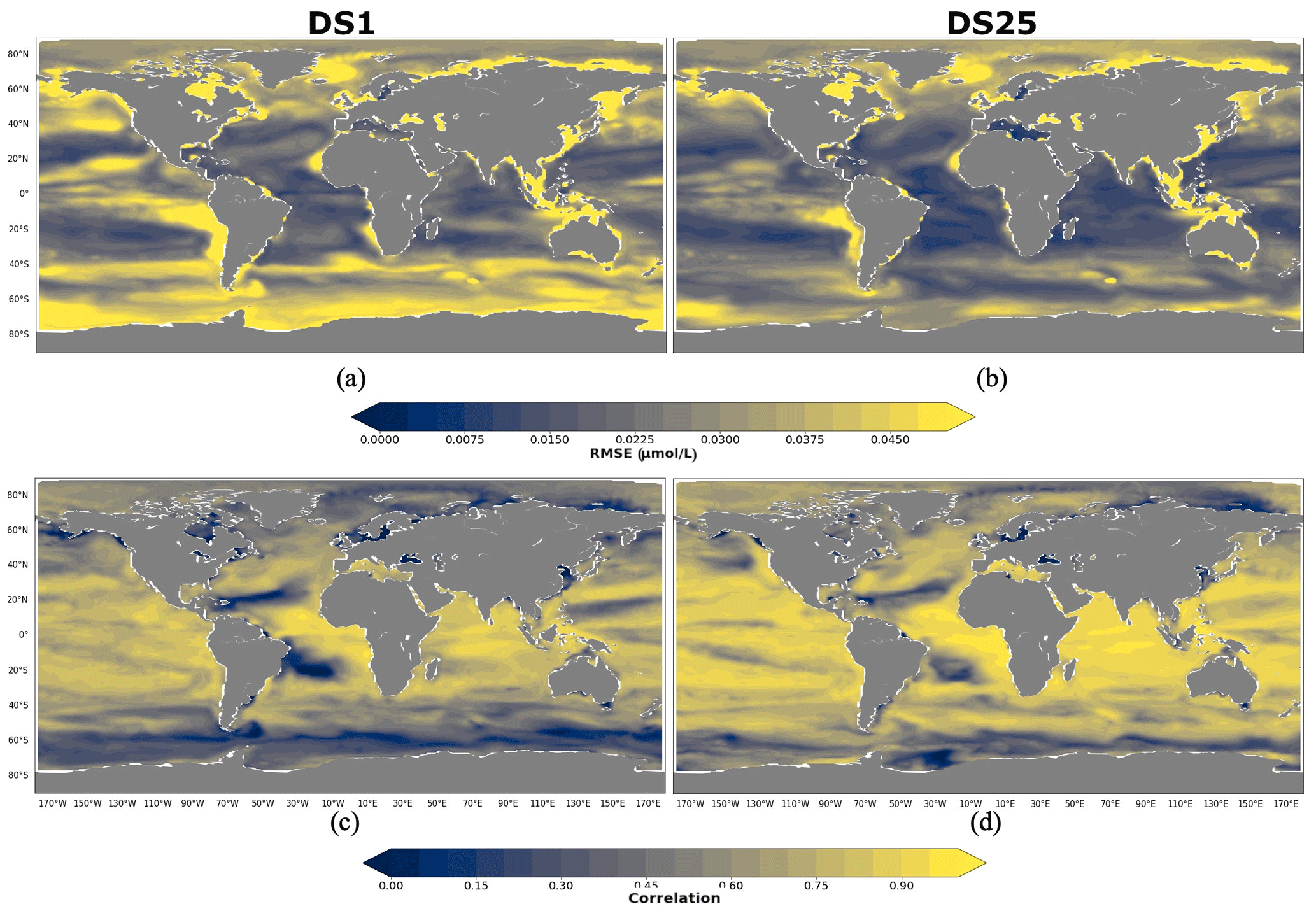
Figure 11 RMSE and correlation between monthly PlankTOM12 and results of POC_L reconstruction using XGBoost over the period 2009–2013 for POC_L. (a, b) RMSEs and (c, d) correlation coefficients. (a, c) Reconstruction based on DS1 (NoPFT) and (b, d) reconstruction based on DS25 (vertical profiles of zooplankton as well as zooplankton and phytoplankton averaged over MLD).

Global maps of statistics suggest that the most sensible region to driver sets' composition for POC_L is the Southern Ocean, as for POC_S (Fig. 11). In the 40–60^∘ S region, RMSE is reduced from 0.037 µmol L⁻¹ in DS1 to 0.024 µmol L⁻¹ in DS25 (Fig. 9d), and the correlation coefficient is increased from 0.42 to 0.66 (Fig. 9c) on average, respectively. In the southern region, 60–90^∘ S, RMSE is reduced from 0.047 µmol L⁻¹ in DS1 to 0.033 µmol L⁻¹ in DS25, and the correlation coefficient is increased from 0.33 to 0.42 (Fig. 9c) on average, respectively. The average correlation coefficients in this zone were found to be less than 0.5 in all tests, with the highest value 0.5 in DS21. DS21 contains all PFTs and chlorophyll a vertical profile as drivers. The RMSE for DS21 in this region is close to the one of DS25, 0.34 and 0.33 µmol L⁻¹, respectively. It identifies the importance of chlorophyll a in the Southern Ocean as a driver of POC_L variability.

The statistics of POC_S and POC_L reconstruction do not vary significantly between driver sets in all regions except in the Southern Ocean. This region is most sensitive to the composition of driver sets for both POC_S and POC_L.

4 Conclusions

The aim of this work was to test the potential of using machine learning to reproduce modelled concentrations of particulate organic carbon within the ocean using the distribution of available observations. We co-localized outputs of the PlankTOM12 global biogeochemical ocean model with the positions of observations of small (POC_S) and large (POC_L) particulate organic carbon concentrations. Using PlankTOM outputs as references we could identify the best ML method for POC reconstruction and estimate the method's accuracy in regions with poor observational cover.

We tested two ML methods to reconstruct POC_S and POC_L: the XGBoost regressor and random forest. Both methods are algorithms based on decision trees. XGBoost outperformed random forest by about 9 % on average for POC_S reconstruction and by about 3 % on average for POC_L reconstruction. XGBoost regressor builds the model sequentially, improving it at each iterative step. At each iteration, XGBoost regressor analyses the prediction and gives more weight to the data where the fit is still wrong. It is a good tool for an unbalanced data set, like in our case where the data of particulate organic carbon concentration are sparse in time and space.

We tested the influence of a wide range of environmental and ecosystem drivers on POC_S and POC_L reconstruction. The introduction of plankton functional types (PFTs) in the driver set greatly improves the fit and shows a linkage between surface ecosystem structure and particulate organic carbon distribution within the ocean interior. We improved the accuracy of POC_S reconstruction by 59 % on RMSE and 63 % on absolute bias and by 52 % on correlation by introducing PFTs in the driver sets (from the comparison of DS1 and DS25). The presence of PFTs in the driver sets also improved the accuracy of POC_L reconstruction by 22 % on RMSE, absolute bias and correlation (from the comparison of DS1 and DS25). POC_S variability mostly depends on the depth level and vertical profiles of microzooplankton, temperature and PO₄. POC_L variability depends on the depth level; MLD; chlorophyll a averaged over MLD; and vertical profiles of temperature, microzooplankton, phaeocystis and PO₄. Additionally, we identified that chlorophyll a in driver sets improves the POC_L reconstruction in the Southern Ocean.

Despite the good accuracy over the global ocean on average, the statistics are worse in the coastal regions and in the tropical eastern Pacific. The coastal regions suffer from a lack of data to represent the coastal dynamics. Therefore the ML reconstructions assign open-ocean processes to coastal regions, leading to significant biases. The tropical eastern Pacific is a region of strong interannual variability, and the sparse measurements in time make it harder to capture this variability correctly. Other regions with poor coverage by observations – the eastern Indian Ocean, the western Pacific Ocean and the Southern Ocean – show the statistics of reconstruction comparable to one from regions with a good cover – regions in the Atlantic Ocean. However, we found that the Southern Ocean is a more sensible region to the driver set's composition. The observational data are particularly sparse in this region, and our analysis suggests that identifying the drivers of importance based on real data set will be difficult.

Here we showed that the XGBoost regressor and random forest are suitable for this problem and can reconstruct modelled POC_S and POC_L with appropriate accuracy. This is evidenced from the globally averaged correlation coefficient up to 0.88 for POC_S and 0.68 for POC_L and the globally averaged RMSE up to 20 % (0.08 µmol L⁻¹) of standard deviation of PlankTOM12 POC_S and 65 % (0.028 µmol L⁻¹) of standard deviation of PlankTOM12 POC_L. ML outputs represent the spatial patterns of POC_S and POC_L distribution well. However, the validity of the approach on observations is dependent on the availability of co-located information on the drivers of importance. For some drivers this should be possible (e.g. environmental conditions and chlorophyll a), while for other drivers information is more sparse (e.g. the PFTs). Our analysis suggests that additional PFT observations would help provide broader insights into the distribution of POC in the ocean. The next step of this work is to apply ML to real data using methods from the present study. Testing the present ML approach on observations will also help provide suggestions for an optimal set of drivers that can be measured specifically for POC reconstruction. For example, based on model results only, our results suggest that microzooplankton concentration is particularly important and should be measured more systematically, especially in the regions of high interannual variability. Likewise, this work provides information on the variables that are less important in POC variability, like vertical profiles of gelatinous zooplankton or mixed phytoplankton for POC_S and coccolithophore for POC_L, and, thus, less important to be measured in this context. These results will need to be tested with observations before firmly confirming the validity of the drivers. The validated driver sets can help guide observational programmes. In addition, recent advances in plankton imaging (Irisson et al., 2022; Lombard et al., 2019; Orenstein et al., 2022) and omics (Faure et al., 2021) will soon provide a new global set of data to estimate PFT concentrations across ocean basins, allowing us to better identify potential biological drivers of POC variability. The new available data of PFTs will significantly facilitate the application of ML methods, such as the one developed here, to observational data.

The relationships between key variables and surrounding conditions based on machine learning can provide a new way for establishing parameters in ocean model parameterization. The parameters can be time- and space-dependent and, thus, vary from one region to another, better representing the physics. The relationship between POC concentration and environmental and ecosystem conditions can help to replace parameters in parameterized sinking velocity in PlankTOM. The reconstructed POC concentration over the global ocean will contribute to the reconstruction of porosity and opacity of particles that are key variables in the sinking matter velocity.

This study provides insights on the drivers that may be responsible for POC_S and POC_L variability and regional dependencies. However, the dependencies are simply returning the outcome of complex ecosystem processes among the drivers as represented in the PlankTOM12 model. Although these processes are based on current understanding and a broad range of observations (Le Quéré et al., 2016; Wright et al., 2021; Buitenhuis et al., 2019), they remain results from a model output. Observations could reveal different drivers that are important for POC_S and POC_L. Depending on data availability and their time and space resolution, the final product based on observations should provide new insights on the drivers that govern particulate organic carbon concentration in the real ocean.