Tracing and visualisation of contributing water sources in the LISFLOOD-FP model of flood inundation (within CAESAR-Lisflood version 1.9j-WS)

We describe the formulation of a simple method of water source tracing for computational models of flood inundation and demonstrate its implementation within CAESAR-Lisflood. Water source tracing can provide additional insight into flood dynamics by accounting for flow pathways of each model boundary condition. The method developed is independent of the hydraulic formulation used, allowing it to be implemented in other model codes without affecting flow routing. In addition, we developed a method which allows up to three water sources to be visualised in the RGB colour space, while continuing to allow depth to be resolved. The number of water sources that may be traced is limited only by the computational resources. We show the application of the methods developed for example applications of a major flood event, a shallow estuary, and Amazonian wetland inundation. A key advantage is that the method is independent of the hydraulic formulation, meaning that it is relatively straightforward to add to existing finite-volume codes, including those based on or developed around the LISFLOOD-FP method. This method enables water tracing with a minimal computational overhead, allowing users of the LISFLOOD-FP method to address environmental issues relating to water sources and mixing, such as water quality and contamination problems.

1 Introduction

Flood inundation models relate upstream river inflow and other dynamic boundary conditions (e.g. downstream stage) to inundation extent, depth, and velocity and have become invaluable tools for the assessment and understanding of flood dynamics and risk. Recently, a series of fast and effective two-dimensional (2D) hydrodynamic models have been developed (Hunter et al., 2007; Neal et al., 2018). These model codes have enabled the assessment of flood inundation at high spatial resolutions (e.g. Yu and Coulthard, 2015) and large spatial scales, including applications on the Amazon (Wilson et al., 2007) and Congo (O'Loughlin et al., 2020), at continental scales (Dottori et al., 2022; Wing et al., 2017), and global scales (Dottori et al., 2016; Sampson et al., 2015). The LISFLOOD-FP model (Bates and De Roo, 2000; Bates et al., 2010) uses a fixed raster grid structure and includes several flow formulations of different physical complexity (Shaw et al., 2021), which have been widely used for flood hazard assessment in fluvial (Horritt et al., 2010) and coastal (Vousdoukas et al., 2018) applications, in addition to within models of landscape evolution (Adams et al., 2017; Coulthard et al., 2013). However, the ability to trace the sources of water in the model domain is presently missing from reduced-complexity 2D flood models such as LISFLOOD-FP.

Understanding the contribution of different water sources to flooding and river flows is important when managing river basins by, for example, determining the relative contribution of tributaries or where waterborne contamination is an issue. This is a function found in more complex two- and three-dimensional models based on the full shallow water equations, such as TELEMAC (Galland et al., 1991) and Ansys Fluent, and has been used for a variety of applications, including water quality modelling in a lake (Kopmann and Markofsky, 2000) and solute and viral dispersal in estuaries (Robins et al., 2014, 2019). For example, in TELEMAC, non-buoyant tracers can be added and their course and concentration followed (Sect. 9; Ata et al., 2014). Similarly, in PCSWMM, Qi et al. (2021) and Qi et al. (2022) developed a module to assess the relative contributions to downstream flood waters from upstream source catchments, with tracer sources generated by the PCSWMM water quality routing module. In their approach, each upstream source is assigned a constant tracer concentration, which is then routed downstream using PCSWMM methods for the transportation of pollutants. The source proportion for a downstream catchment is then determined from the relative mass of the total tracer amount which is in that catchment and multiplied by the total flood volume. However, approaches using such 2D and 3D codes have a considerable computational overhead compared to simpler schemes such as LISFLOOD-FP.

In this paper, we build on the work of Wilson and Coulthard (2019) to propose a simple and efficient method which can be added to finite-volume codes to track the contribution of multiple water sources to predicted flood depths without the addition of tracers and demonstrate it within the CAESAR-Lisflood model (Coulthard et al., 2013) for several example flooding case studies which each represent the mixing of water from multiple sources. CAESAR-Lisflood (available from https://sourceforge.net/projects/caesar-lisflood/, last access: 25 April 2023) is a development of the CAESAR model (Coulthard et al., 2002; Van De Wiel et al., 2007) and the LISFLOOD-FP 2D hydrodynamic model (Bates et al., 2010) that simulates landscape evolution by coupling a hydrological model, a surface water flow model, fluvial erosion and deposition, and slope processes.

In earlier work with CAESAR, Coulthard and Macklin (2003) demonstrated how sediment eroded from mining waste deposits could be traced downstream. The model worked by including different types of sediments which were used to represent contaminated and uncontaminated sediments as separate arrays for each sediment diameter included; during the erosion and deposition of different sediment sizes, equal proportions of contaminated and uncontaminated sediment were transported. This enabled the prediction of patterns and levels of floodplain contamination over a period of ∼400 years. However, the approach was limited to sediment tracing only and did not account for different sources of water, which may carry contaminants with it. As noted by Coulthard et al. (2013), the inclusion of an unsteady flow formula within CAESAR-Lisflood has enabled the possibility, for example, to simulate water balances and solute fluxes using the model code. Here, we present the formulation of a simple methodology to enable this functionality by accounting for the source of water within model cells throughout the simulation.

We use only the hydraulic and hydrological functionality of CAESAR-Lisflood to demonstrate the tracing method and visualisation of water sources independently of sediment routing. We have used CAESAR-Lisflood for this purpose, as the software is fully open source, integrating a graphical user interface (GUI) in addition to the hydraulic methods from LISFLOOD-FP. This enables our visualisation methods to be incorporated but does not limit our tracing method to CAESAR-Lisflood. The equations and pseudo-code examples provided make it a straightforward task for users and researchers to add this functionality to LISFLOOD-FP (and other variants using similar methods).

2 Methods

2.1 Flow formulation

CAESAR-Lisflood implements the LISFLOOD-FP inertial formulation (Bates et al., 2010) to estimate depths across the domain. This is a reduced physical complexity, mass conservative hydraulic model structured on a Cartesian grid in which the updated water depth h, at time t and for cell i,j, is determined using the following (Bates and De Roo, 2000):

$$\begin{array}{}\text{(1)}& h_{i,j}^t=h_{i,j}^{t-\mathrm{\Delta }t}+\mathrm{\Delta }t{\displaystyle \frac{Q_{x,i-\mathrm{1},j}^t-Q_{x,i,j}^t+Q_{y,i,j-\mathrm{1}}^t-Q_{y,i,j}^t}{\mathrm{\Delta }{x}^{\mathrm{2}}}},\end{array}$$

where $h_{i,j}^{t-\mathrm{\Delta }t}$ is the cell depth at the end of the previous time step (Δt), Q represents the flows into or out of the cell in the x or y directions, and Δx is the cell size. Flows are decoupled in each direction. Flow in the x direction is determined using the following (de Almeida et al., 2012; Bates et al., 2010):

$$\begin{array}{}\text{(2)}& Q_x^t={\displaystyle \frac{q_x^{t-\mathrm{\Delta }t}-g{h}_{\left[\text{flow}\right]}^t\mathrm{\Delta }t\frac{\mathrm{\Delta }(h^t+z)}{\mathrm{\Delta }x}}{(\mathrm{1}+g{h}_{\left[\text{flow}\right]}^t\mathrm{\Delta }t{n}^{\mathrm{2}}|q_x^{t-\mathrm{\Delta }t}|/(h_{\left[\text{flow}\right]}^t{)}^{\mathrm{10}/\mathrm{3}})}}\mathrm{\Delta }y,\end{array}$$

with flow in the y direction obtained analogously. In Eq. (2), $q_x^{t-\mathrm{\Delta }t}$ represents the flux between the cells from the previous time step ($Q_x^{t-\mathrm{\Delta }t}/\mathrm{\Delta }y$), g is acceleration from gravity, h_[flow] is the maximum depth of flow between two cells, n is Manning's roughness, and z is the cell bed elevation. The LISFLOOD-FP inertial formulation has been benchmarked against other formulations and industry standard codes and showed that, in appropriate flow conditions (i.e. gradually varied flow; Froude number $<\sim \mathrm{1}$), the model performed favourably and with high efficiency (de Almeida and Bates, 2013; Neal et al., 2012).

2.2 Water source tracing

Given that the sum of depths in a cell from each source, w, make up its total flood depth, h,

$$\begin{array}{}\text{(3)}& \sum _{w=\mathrm{1}}^W{h}_w=h\text{,}\end{array}$$

the volume fraction of each source, ϕ_w, may be obtained from

$$\begin{array}{}\text{(4)}& {\mathit{\varphi }}_w={\displaystyle \frac{h_w}{h}}\text{,}\end{array}$$

ensuring

$$\begin{array}{}\text{(5)}& \sum _{w=\mathrm{1}}^W{\mathit{\varphi }}_w=\mathrm{1}\text{.}\end{array}$$

Thus, the fraction of each water source in each cell is defined as the depth of water from that source in the cell divided by the total cell depth.

Following this, once flows between cells are calculated and depths updated, our water tracing method proceeds as follows. (1) For each cell, the remaining depth following removal of water from any outflows is found. (2) The amount of the depth belonging to each water source is obtained by scaling the depths according to water source fractions from the previous time step. (3) Contributing inflow depths from each source for all neighbours is added to each source depth. (4) Updated water source fractions are calculated, as per Eq. (4), by dividing the fractions from each source by the updated total cell depth. More formally, for each cell, for each water source, w, at time, t, the volume fraction ϕ is as follows:

$$\begin{array}{}\text{(6)}& {\mathit{\varphi }}_w^t={\displaystyle \frac{h_{Q_{\left[\text{out}\right]}}^t{\mathit{\varphi }}_w^{t-\mathrm{\Delta }t}+{\sum }_D\left(Q_{\left[\text{in}\right]}^{t,D}{\mathit{\varphi }}_w^{t-\mathrm{\Delta }t,D}\right)\frac{\mathrm{\Delta }t}{\mathrm{\Delta }{x}^{\mathrm{2}}}}{h^t}},\end{array}$$

where $h_{Q_{\left[\text{out}\right]}}^t$ represents the depth remaining in the cell after the removal of outflows at the current time, $Q_{\left[\text{out}\right]}^t$ (and before the addition of any inflows), which is scaled according to the fraction from this source from the previous time step, ${\mathit{\varphi }}_w^{t-\mathrm{\Delta }t}$. To this depth the total amount of water from this source is added, which is contributed from neighbouring cells and given by ${\sum }_D\left(Q_{\left[\text{in}\right]}^{t,D}{\mathit{\varphi }}_w^{t-\mathrm{\Delta }t,D}\right)$, where $Q_{\left[\text{in}\right]}^{t,D}$ is the inflow from a particular direction, D, and ${\mathit{\varphi }}_w^{t-\mathrm{\Delta }t,D}$ is the fraction of flow for source, w, from that direction. The updated source volume fraction is obtained by dividing by the updated cell depth, h^t. Finally, $h_{Q_{\left[\text{out}\right]}}^t$ is given by the following:

$$\begin{array}{}\text{(7)}& h_{Q_{\left[\text{out}\right]}}^t=h^{t-\mathrm{\Delta }t}-\sum _D{Q}_{\left[\text{out}\right]}^{t,D}{\displaystyle \frac{\mathrm{\Delta }t}{\mathrm{\Delta }{x}^{\mathrm{2}}}},\end{array}$$

where $Q_{\left[\text{out}\right]}^{t,D}$ are the outflows in each direction. To improve the computational efficiency, the method only requires knowledge of the source volume fractions for the previous time step in each neighbouring, upstream cell; the actual depths or volumes from each source in each cell are not saved. The calculation cell depth after the removal of outflows, $h_{Q_{\left[\text{out}\right]}}^t$, enables each source fraction to be updated based on the flows in ($Q_{\left[\text{in}\right]}^{t,D}$), the fraction from each source in direction, D (${\mathit{\varphi }}_w^{t-\mathrm{\Delta }t,D}$), and the updated depth, h^t. Using this approach, the calculation of water source fractions flowing out of the cell is not necessary. For completeness, using the notation of Eq. (1) and expanding D into cell indices, i,j, the updated depth from each source can be obtained using the following:

$$\begin{array}{}\text{(8)}& \begin{array}{rl}& {\mathit{\varphi }}_{w,i,j}^t{h}_{i,j}^t={\mathit{\varphi }}_{w,i,j}^{t-\mathrm{\Delta }t}{h}_{i,j}^{t-\mathrm{\Delta }t}\\ & +\mathrm{\Delta }t{\displaystyle \frac{{\mathit{\varphi }}_{w,i-\mathrm{1},j}^{t-\mathrm{\Delta }t}{Q}_{x,i-\mathrm{1},j}^t-{\mathit{\varphi }}_{w,i+\mathrm{1},j}^{t-\mathrm{\Delta }t}{Q}_{x,i,j}^t+{\mathit{\varphi }}_{w,i,j-\mathrm{1}}^{t-\mathrm{\Delta }t}{Q}_{y,i,j-\mathrm{1}}^t-{\mathit{\varphi }}_{w,i,j+\mathrm{1}}^{t-\mathrm{\Delta }t}{Q}_{y,i,j}^t}{\mathrm{\Delta }{x}^{\mathrm{2}}}}\text{.}\end{array}\end{array}$$

Boundary condition inputs are added prior to the routing of surface water. Adjusting the water volume fractions for the cells in which water is added is straightforward. The boundary-modified water volume fractions, ${\mathit{\varphi }}_w^{\prime }$, are obtained using

$$\begin{array}{}\text{(9)}& {\mathit{\varphi }}_w^{\prime }={\displaystyle \frac{h{\mathit{\varphi }}_w+Q_w\frac{\mathrm{\Delta }t}{\mathrm{\Delta }{x}^{\mathrm{2}}}}{h+{\sum }_w{Q}_w\frac{\mathrm{\Delta }t}{\mathrm{\Delta }{x}^{\mathrm{2}}}}}\end{array}$$

for input sources or

$$\begin{array}{}\text{(10)}& {\mathit{\varphi }}_w^{\prime }={\displaystyle \frac{h{\mathit{\varphi }}_w}{h+{\sum }_w{Q}_w\frac{\mathrm{\Delta }t}{\mathrm{\Delta }{x}^{\mathrm{2}}}}}\end{array}$$

for other sources, where Q_w is the inflow added to the cell from source w at the start of the time step. Thus, fractions from sources where water is added to the cell are adjusted upwards, while fractions for non-source volumes are adjusted downwards. This means that additional inflow from a certain source results in an increase in the fraction of that source in that cell, which is reflected in a higher value of the water source fraction variable, ${\mathit{\varphi }}_w^{\prime }$; the opposite occurs for fractions of water from other sources, as they are diluted.

It should be noted that, similar to the approach of Qi et al. (2021), for simplicity, this method treats cell water volumes as being fully mixed. Consequently, it may be possible for small fractions to propagate quickly in a downstream direction, since fluxes into a cell would be included in the fractions assigned as inflow to a downstream neighbouring cell in the next time step via ${\mathit{\varphi }}_w^{t-\mathrm{\Delta }t,D}$. As a result, caution should be given to the interpretation of very small water source fractions.

2.3 Water tracing implementation

Importantly, within the model code, the additional equations required for the water source tracing presented in Sect. 2.2 can be piggybacked on top of the existing finite-volume model code, requiring minimal modification of the original schemes. The water source tracing method was implemented in C#, building from the code base in CAESAR-Lisflood version 1.9j (Coulthard, 2019). However, the method is readily transferable to other programming languages, where different versions of LISFLOOD-FP (Bates et al., 2010) are implemented, or to other similar flow models. The additional C# code added to CAESAR-Lisflood is included in Appendix A. Here, we summarise the algorithms developed.

Our method allows water from different sources to be tracked according to point sources (e.g. a reach input) or from spatial areas that can be user-defined (e.g. to represent different rain zones or subcatchments). CAESAR-Lisflood allows the addition of water as point sources or via rainfall through a hydrological model based on a spatially distributed version of TOPMODEL (Beven and Kirkby, 1979; for implementation, see Coulthard and Skinner, 2016, and Coulthard and Van De Wiel, 2017). The zonal input also allows tidal sources to be traced, although it is worth noting that the model is depth-averaged and does not account for the higher density of saltwater. Water tracers are saved as two 3D or stacked arrays of grid cells sized $W\times X\times Y$ for the current and previous time step, which are initialised as zeros. Additionally, two arrays for δhδt in the x and y directions are used to save the volumes of water moving between cells in units of change in depth in the time step.

The main functional flow of CAESAR-Lisflood, as related to water source tracing, is shown in Fig. 1. For each time step, inflows from various sources are first added. The addition of traced water requires the code to be modified such that, after the addition of water from each source, the water source fractions are updated to account for the increase in volume from a source (Eqs. 9 and 10). In CAESAR-Lisflood, inflows to the modelled domain may reflect reach inputs, rainfall inputs, and tidal or stage inputs, which are added in three separate functions (reach_water_and_sediment_input(), catchment_water_input_and_hydrology() and stage_tidal_input(), respectively). Each of these are updated in a similar way, using Algorithm 1.

Following the addition of inputs from sources, the implementation in CAESAR-Lisflood copies the water depths and water tracers into arrays which represent the previous time step, h_t−1 and ϕ_t−1. For the water source tracing implementation, the tracer states are saved via the function save_tracer_states() (Fig. A3). Next, flows are updated in the function qroute(), for which no modifications are required (meaning that the water source tracing does not affect flow). Depths are then updated via depth_update() with no modifications, except that the volumes of water moving between cells are stored to the δhδt in x and y arrays, which are calculated using

$$\begin{array}{}\text{(11)}& \mathit{\delta }h\mathit{\delta }{t}^{t,D}=Q^{t,D}{\displaystyle \frac{\mathrm{\Delta }t}{\mathrm{\Delta }x}}\end{array}$$

for a single direction (C# code in Fig. A4). This is used as part of the solution to Eqs. (6) and (7) to update the water source tracers, enabling a simplified form to be implemented for the tracer update as follows:

$$\begin{array}{}\text{(12)}& {\mathit{\varphi }}_w^t={\displaystyle \frac{h_{Q_{\left[\text{out}\right]}}^t{\mathit{\varphi }}_w^{t-\mathrm{\Delta }t}+{\sum }_D\left(\mathit{\delta }h\mathit{\delta }{t}_{\left[\text{in}\right]}^{t,D}{\mathit{\varphi }}_w^{t-\mathrm{\Delta }t,D}\right)}{h^t}},\end{array}$$

where

$$\begin{array}{}\text{(13)}& h_{Q_{\left[\text{out}\right]}}^t=h^{t-\mathrm{\Delta }t}-\sum _D\mathit{\delta }h\mathit{\delta }{t}_{\left[\text{out}\right]}^{t,D}\text{.}\end{array}$$

Water source tracers are updated in the function update_tracer_states(), which is the main addition to the CAESAR-Lisflood code. Algorithm 2 provides the details of the procedure used. For every cell in the model which contains water ($h_{i,j}^t>\mathrm{0.0}$), the depth remaining in the cell after the outflows ($h_{Q_{\left[\text{out}\right]}}^t$) is first calculated by subtracting the outflows from each of the four flow directions. We sum δhδt from each direction (previously calculated in depth_update()), which represents the contributions to depth from the right (x) or up (y). Thus, outflows will be negative for the right and upward directions and positive in the left and downward directions.

The procedure then updates each source for the cell by first calculating the sum of depths added from this source (i.e. ${\sum }_D\left(\mathit{\delta }h\mathit{\delta }{t}_{\left[\text{in}\right]}^{t,D}{\mathit{\varphi }}_w^{t-\mathrm{\Delta }t,D}\right)$), which is again done by scanning the δhδt arrays in each direction. Finally, the fraction is calculated by dividing the total new depth from the source by the depth from all sources, h^t.

Algorithm 1 Updating water source fractions after adding the input sources. Inputs required are the depth in the cell for the previous iteration (h^t−1), a vector of all water sources for the cell for the previous iteration (ϕ^t−1), input from this source (Q_w), the index of this source (w), the number of sources (W), the cell size (Δx), and the time step (Δt). A C# implementation is shown in Fig. A2.

Input: h^t−1, ϕ^t−1, Q_w, w, W, Δx, Δt

Output: ϕ^t

$\mathit{\delta }h\mathit{\delta }{t}_w\leftarrow Q_w\cdot \mathrm{\Delta }t/\mathrm{\Delta }{x}^{\mathrm{2}}$ {get change in depth resulting from this source}

$h^t\leftarrow h^{t-\mathrm{1}}+\mathit{\delta }h\mathit{\delta }{t}_w$ {get new depth after adding input from this source}

if h^t>0.0 then

if h^t=δhδt_w then

${\mathit{\varphi }}_w^t\leftarrow \mathrm{1.0}$ {if depth was zero, then all water in cell is from this source}

else if ${\mathit{\varphi }}_w^{t-\mathrm{1}}<\mathrm{1.0}$ {if cell contains multiple sources} then

$h_w^t\leftarrow {\mathit{\varphi }}_w^{t-\mathrm{1}}\cdot h^{t-\mathrm{1}}$ {get depth after addition of this source}

${\mathit{\varphi }}_w^t\leftarrow (h_w^t+\mathit{\delta }h\mathit{\delta }{t}_w)/h^t$ {update this water source fraction}

for src=1 to W do

if src≠w then

${\mathit{\varphi }}_{\mathrm{src}}^t\leftarrow ({\mathit{\varphi }}_{\mathrm{src}}^{t-\mathrm{1}}\cdot h^{t-\mathrm{1}})/h^t$ {update fraction of other water sources}

end if

end for

end if

end if

Algorithm 2 Updating water source fractions after the flow routing and depth update. Inputs required are the updated depth in the cell (h^t), water sources for the previous iteration (ϕ^t−1), depth contributions horizontally (δhδtx) and vertically (δhδty), the number of sources (W), and the number of cells in the grid horizontally (X) and vertically (Y). A C# implementation is shown in Fig. A5.

Input: h^t, ϕ^t−1, δhδtx, δhδty, W, X, Y

Output: ϕ^t

for all i, j cells in ranges $\mathrm{1}\le i\le X$ and $\mathrm{1}\le j\le Y$ do

if $h_{i,j}^t>\mathrm{0.0}$ then

$\mathit{\delta }h\mathit{\delta }t{\text{sum}}_{Q_{\left[\text{out}\right]}}\leftarrow \mathrm{0.0}$ {obtain total change in depth after flows out (source not important)}

if $\mathit{\delta }h\mathit{\delta }t{x}_{i+\mathrm{1},j}<\mathrm{0.0}$, then $\mathit{\delta }h\mathit{\delta }t{\text{sum}}_{Q_{\left[\text{out}\right]}}\leftarrow \mathit{\delta }h\mathit{\delta }t{\text{sum}}_{Q_{\left[\text{out}\right]}}+\mathit{\delta }h\mathit{\delta }t{x}_{i+\mathrm{1},j}$; end if {right, −ve = outflow}

if $\mathit{\delta }h\mathit{\delta }t{x}_{i,j}>\mathrm{0.0}$, then $\mathit{\delta }h\mathit{\delta }t{\text{sum}}_{Q_{\left[\text{out}\right]}}\leftarrow \mathit{\delta }h\mathit{\delta }t{\text{sum}}_{Q_{\left[\text{out}\right]}}-\mathit{\delta }h\mathit{\delta }t{x}_{i,j}$;     end if {left, +ve = outflow}

if $\mathit{\delta }h\mathit{\delta }t{y}_{i,j+\mathrm{1}}<\mathrm{0.0}$, then $\mathit{\delta }h\mathit{\delta }t{\text{sum}}_{Q_{\left[\text{out}\right]}}\leftarrow \mathit{\delta }h\mathit{\delta }t{\text{sum}}_{Q_{\left[\text{out}\right]}}+\mathit{\delta }h\mathit{\delta }t{y}_{i,j+\mathrm{1}}$; end if {up, −ve = outflow}

if $\mathit{\delta }h\mathit{\delta }t{y}_{i,j}>\mathrm{0.0}$, then $\mathit{\delta }h\mathit{\delta }t{\text{sum}}_{Q_{\left[\text{out}\right]}}\leftarrow \mathit{\delta }h\mathit{\delta }t{\text{sum}}_{Q_{\left[\text{out}\right]}}-\mathit{\delta }h\mathit{\delta }t{y}_{i,j}$;     end if {down, +ve = outflow}

$h_{Q_{\left[\text{out}\right]}}^t\leftarrow h^{t-\mathrm{1}}+\mathit{\delta }h\mathit{\delta }t{\text{sum}}_{Q_{\left[\text{out}\right]}}$ {get depth remaining in cell after removal of outflows}

for src=1 to W do

$\mathit{\delta }h\mathit{\delta }t{\text{sum}}_{Q_{\left[\text{in}\right]}}\leftarrow \mathrm{0.0}$ {obtain total change in depth after for inflows of this source (ignoring outflows)}

if $\mathit{\delta }h\mathit{\delta }t{x}_{i+\mathrm{1},j}>\mathrm{0.0}$, then $\mathit{\delta }h\mathit{\delta }t{\text{sum}}_{Q_{\left[\text{in}\right]}}\leftarrow \mathit{\delta }h\mathit{\delta }t{\text{sum}}_{Q_{\left[\text{in}\right]}}+\mathit{\delta }h\mathit{\delta }t{x}_{i+\mathrm{1},j}\cdot {\mathit{\varphi }}_{i+\mathrm{1},j,\mathrm{src}}^{t-\mathrm{1}}$; end if {right, +ve = inflow}

if $\mathit{\delta }h\mathit{\delta }t{x}_{i,j}<\mathrm{0.0}$, then $\mathit{\delta }h\mathit{\delta }t{\text{sum}}_{Q_{\left[\text{in}\right]}}\leftarrow \mathit{\delta }h\mathit{\delta }t{\text{sum}}_{Q_{\left[\text{in}\right]}}-\mathit{\delta }h\mathit{\delta }t{x}_{i,j}\cdot {\mathit{\varphi }}_{i-\mathrm{1},j,\mathrm{src}}^{t-\mathrm{1}}$; end if {left, −ve = inflow}

if $\mathit{\delta }h\mathit{\delta }t{y}_{i,j+\mathrm{1}}>\mathrm{0.0}$, then $\mathit{\delta }h\mathit{\delta }t{\text{sum}}_{Q_{\left[\text{in}\right]}}\leftarrow \mathit{\delta }h\mathit{\delta }t{\text{sum}}_{Q_{\left[\text{in}\right]}}+\mathit{\delta }h\mathit{\delta }t{y}_{i,j+\mathrm{1}}\cdot {\mathit{\varphi }}_{i,j+\mathrm{1},src}^{t-\mathrm{1}}$; end if {up, +ve = inflow}

if $\mathit{\delta }h\mathit{\delta }t{y}_{i,j}<\mathrm{0.0}$, then $\mathit{\delta }h\mathit{\delta }t{\text{sum}}_{Q_{\left[\text{in}\right]}}\leftarrow \mathit{\delta }h\mathit{\delta }t{\text{sum}}_{Q_{\left[\text{in}\right]}}-\mathit{\delta }h\mathit{\delta }t{y}_{i,j}\cdot {\mathit{\varphi }}_{i,j-\mathrm{1},\mathrm{src}}^{t-\mathrm{1}}$; end if {down, −ve = inflow}

if $\mathit{\delta }h\mathit{\delta }t{\text{sum}}_{Q_{\left[\text{in}\right]}}=\mathrm{0}$ and ${\mathit{\varphi }}_{\mathrm{src}}^{t-\mathrm{1}}=\mathrm{0}$ then

${\mathit{\varphi }}_{i,j,\mathrm{src}}^t\leftarrow \mathrm{0.0}$ {if there is no contribution or existing water from this source}

else

${\mathit{\varphi }}_{i,j,\mathrm{src}}^t\leftarrow (h_{Q_{\left[\text{out}\right]}}^t\cdot {\mathit{\varphi }}_{i,j,\mathrm{src}}^{t-\mathrm{1}})+\mathit{\delta }h\mathit{\delta }t{\text{sum}}_{Q_{\left[\text{in}\right]}}/h_{i,j}^t$ {([src depth in cell] + [src depth added]) / [updated depth]}

end if

end for

end if

end for

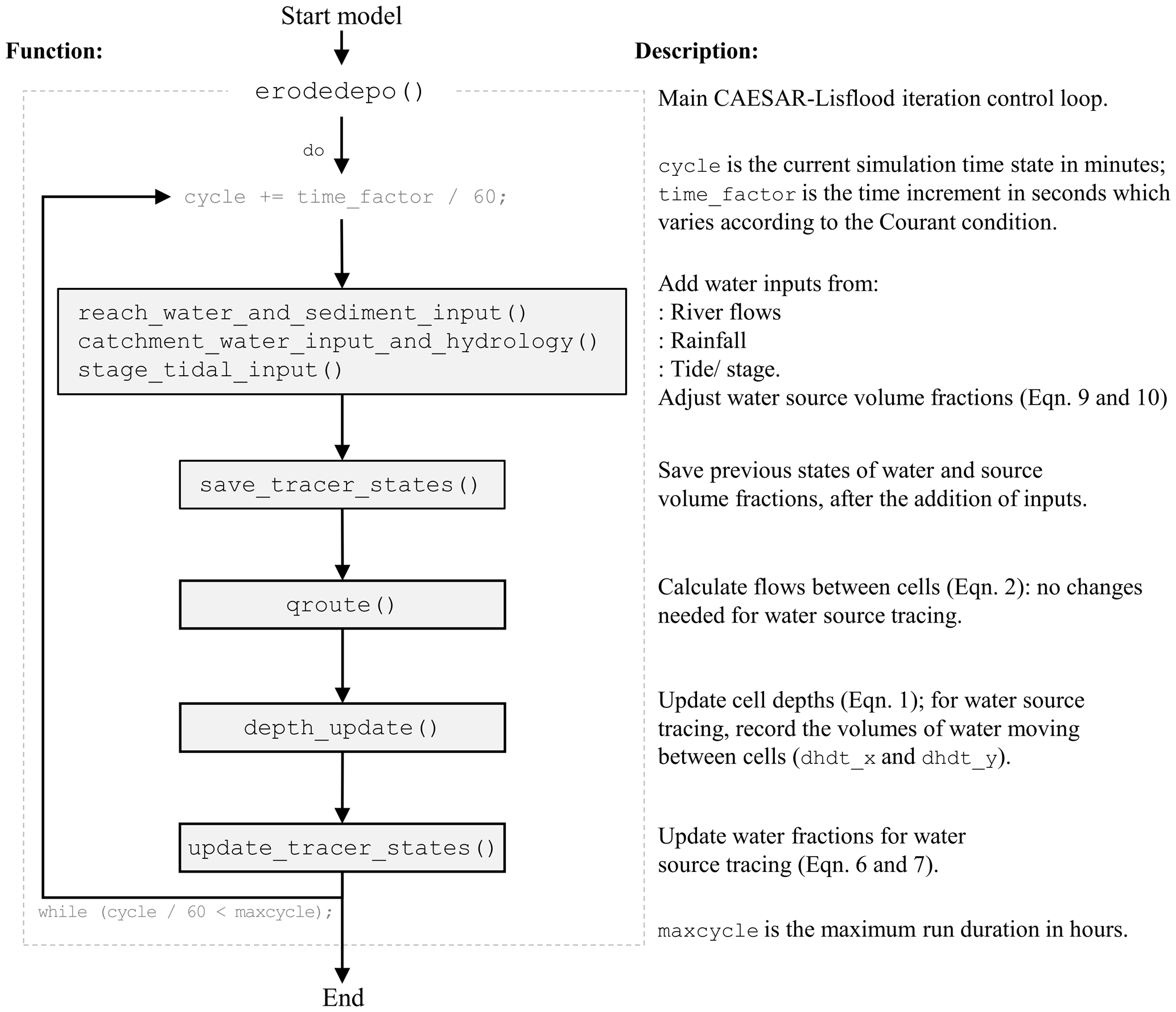
Figure 1 The main CAESAR-Lisflood control showing additions for water source tracing. Additional functions related to erosion and deposition are not shown.

2.4 Water source visualisation

Visualisations of the flood model outputs are often produced for depths in the form of animated maps. Here, we derived a simple colour scaling which permits up to three water sources to be visualised in the RGB colour space. For each cell, the RGB colour index in the range 0 to 255 is obtained for the desired water source, w, using the following:

$$\begin{array}{}\text{(14)}& {\text{RGB}}_{i,j}=\mathrm{255}\cdot {\mathit{\varphi }}_{i,j,w}^{\mathit{\beta }}.\end{array}$$

The power term, β, enables a visual enhancement of the lower water fractions in the range ∼0.1 to 1.0, where 1 would represent no enhancement. In order to allow water depth to be resolved through the use of reduced lightness for deeper water, Eq. (14) may be modified to the following:

$$\begin{array}{}\text{(15)}& {\text{RGB}}_{i,j}=\left(\right(\mathrm{1}-h_{i,j}/h_{\left[\text{range}\right]})\cdot \mathrm{127})+\mathrm{128}\cdot {\mathit{\varphi }}_{i,j,w}^{\mathit{\beta }},\end{array}$$

where h_i,j is the cell depth, and h_[range] is the range of depths to which the visualisation is scaled. Thus, the RGB value for a cell which only has one source of water in it will range from 128 for deeper water, where h=h_[range], towards 255 for shallow depths close to 0. Figure 2 provides a detailed illustration of the RGB values obtained using Eqs. (14) and (15) for different values of ϕ, β, and h and the resulting colour scales obtained when visualising multiple sources. The mixing of water sources with red and blue shading gives a pink colour scale, green and blue give cyan, red and green give yellow, and shades towards white would indicate the mixing of all three sources. Note that, while it is possible to trace an arbitrary number of water sources using the method described in Sect. 2.2, this visualisation method is limited to a maximum of three water sources. However, using Eq. (15), if a cell only contains water from sources different to those selected for visualisation, then the depths can still be resolved in greyscale in the RGB value range from 0 to 127. This also means that it is possible to visualise only one water source at a time in a selected primary colour.

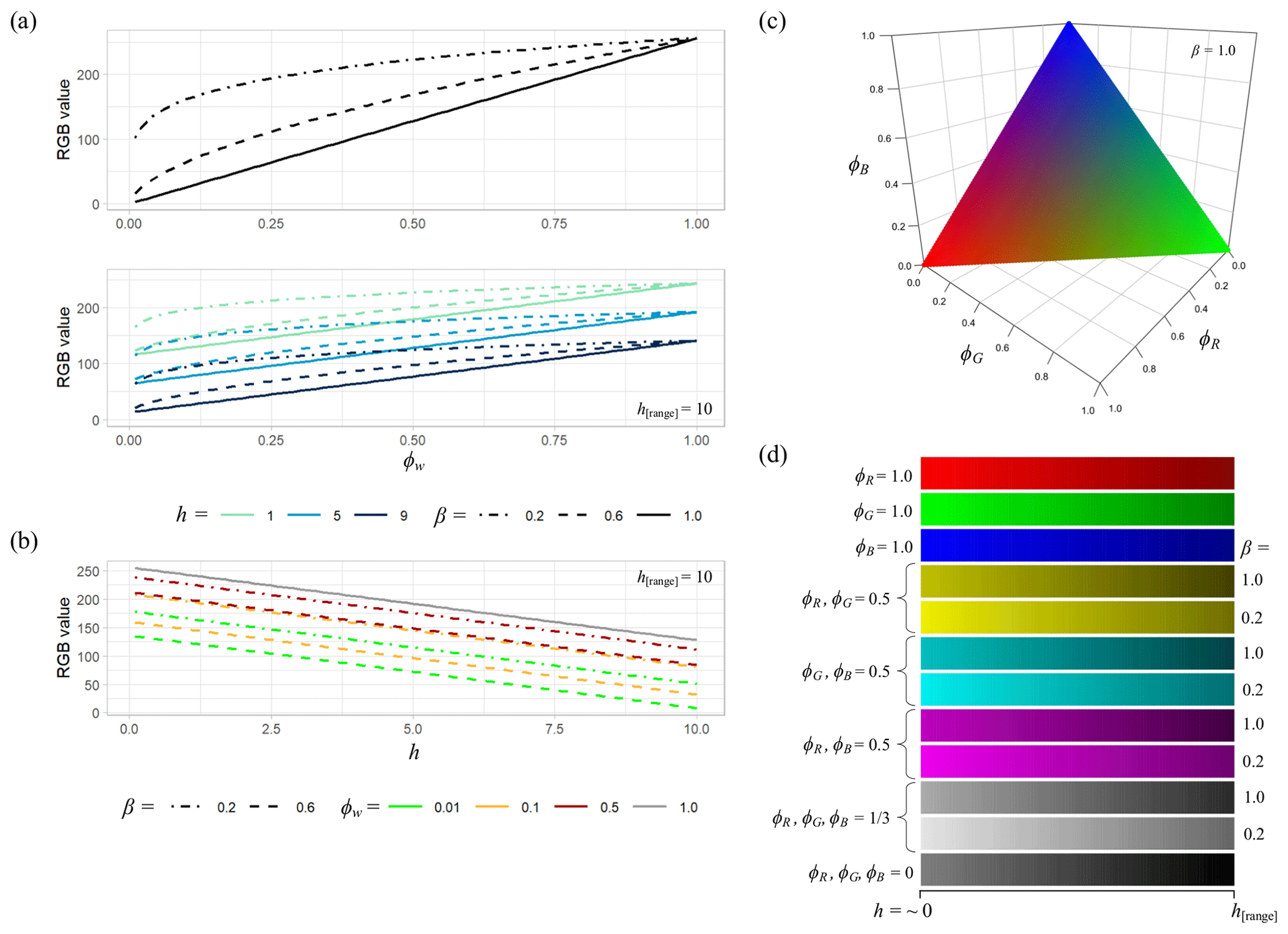
Figure 2 Illustration of the RGB colour scaling used for the visualisation of water source fractions. (a) RGB values for water fractions ϕ from source w, obtained using Eq. (14) (upper plot; no depth visualisation) and Eq. (15) (lower plot, with depth visualisation, where h_[range]=10) and a visual enhancement of lower water fractions using β. (b) RGB values with changing depth, h, for different values of ϕ_w and β. (c) Colour rendering resulting from Eq. (14) for three water sources, R, G, and B (note that ${\mathit{\varphi }}_R+{\mathit{\varphi }}_G+{\mathit{\varphi }}_B=\mathrm{1.0}$). (d) Colour scales obtained for various combinations of water sources using Eq. (15), with and without enhancement of lower water fractions, showing reduced lightness as the water depth approaches h_[range]. Note that the bottom colour scale is used for rendering in the absence of any water from the sources selected for visualisation (i.e. where more than three sources are present in the simulation).

2.5 Evaluating performance overhead

In order to test the computational performance of the water tracing code, a simple planar test case was developed, consisting of a constant 0.001 m m⁻¹ slope of length 2000 m and width 1000 m on a grid with a spatial resolution of 5 m, giving a total of 80 000 cells (Fig. 3a). Manning's roughness, n, was set at 0.05. At 250 m intervals downslope, 1 m “walls” were added across the slope, each with between four and eight gaps of 5 m width added to allow water to flow through. This was done to ensure that water mixed as it flowed downslope. Simulations were conducted for a period of 24 h, with constant inflow of 10 m³ s⁻¹ to eight locations at the top of the slope. Eight simulations were conducted in total, including one with no tracing and seven with between two and eight water sources being traced. To ensure that each of these simulations had identical total inflow, the sources were grouped for tracing purposes, allowing the variation in computation requirements to be assessed. The simulations conducted are summarised in Table 1. Furthermore, to benchmark the model performance in a real-world scenario, the effect of the number of tracers on model performance was tested on the Carlisle example described below.

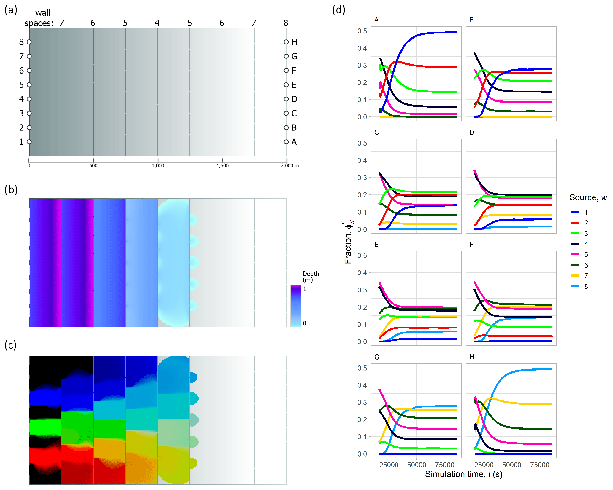
Figure 3 Planar test case set-up and results. (a) The 2000×1000 m planar slope (0.001 m m⁻¹) elevation model (5 m grid spacing; 400×200 cells), with 1 m “walls” added across the slope at 250 m intervals (each wall had between four and eight evenly spaced gaps of 5 m, as indicated by the numbering along the top of the grid). Injection points for each of the eight water sources are indicated by the numbering on the left. (b) Water depth prediction at t=8400 s (140 min), with a constant inflow of 10 m³ s⁻¹ and n=0.05. (c) Visualisation of water sources numbered 2 (red), 4 (green), and 6 (blue) at t=8400 s, using Eq. (14), with β=0.2. (d) Water source fractions throughout the 24 h simulation for each of 1–8 sources at locations A–H, as indicated in panel (a). For an animated version, please see https://youtu.be/DTw8ysJtx8o (last access: 25 April 2023) or the video supplement provided.

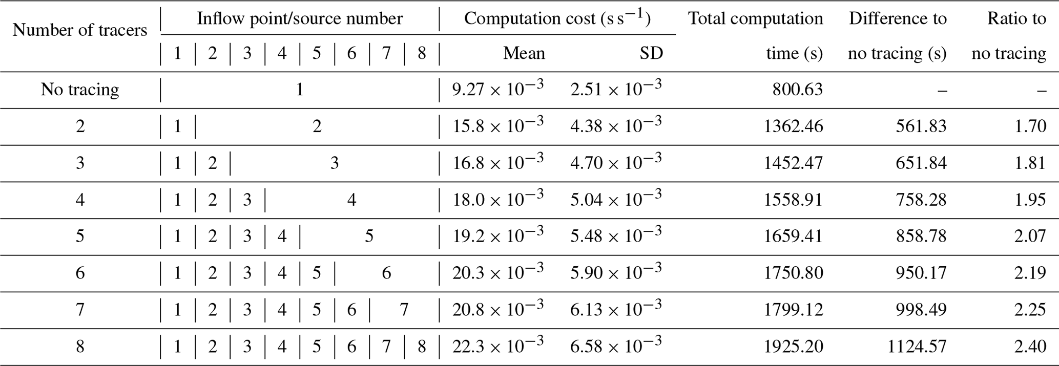
Table 1 Planar slope test case simulations. In each of the eight simulations, the total volume of inflow was identical, and each of the eight sources was a constant 10 m³ s⁻¹ (where a source was used for multiple inflow points, its total volume was added to all). Inflow points are shown in Fig. 3a. Note that SD is the standard deviation.

3 Results

First, we demonstrate water source tracing and visualisation for three flood inundation case studies that are examples of flooding at three different spatial scales in three contrasting contexts, namely (1) a major flood event in 2005 at Carlisle, United Kingdom, which entailed fluvial flooding in an urban area that is situated at the confluence of three rivers, (2) a shallow estuary in Christchurch, New Zealand, combining tides with inflow from two small rivers, and (3) flooding at the tributary junction of two large rivers on the Amazon floodplain, Brazil. Second, we present the computational performance of the method for the planar test case and Carlisle example.

3.1 Carlisle, United Kingdom

The city of Carlisle in northern England experienced significant flooding in 2005 (estimated annual exceedance probability from 0.5 % to 0.57 %) that resulted from heavy rains in the headwater catchments of rivers running through the city and affecting more than 2500 properties (Environment Agency, 2006). With the benefit of an extensive set of observational data obtained from field collection, the 2005 flood event at Carlisle has been used extensively as a test case for hydraulic model development (Horritt et al., 2010; Neal et al., 2009). Here, the site is of particular interest as it is at the confluence of three separate rivers; the main River Eden, which runs from east to west through the city, is joined by the rivers Petteril and Caldew, which flow into the city from the south (Fig. 4).

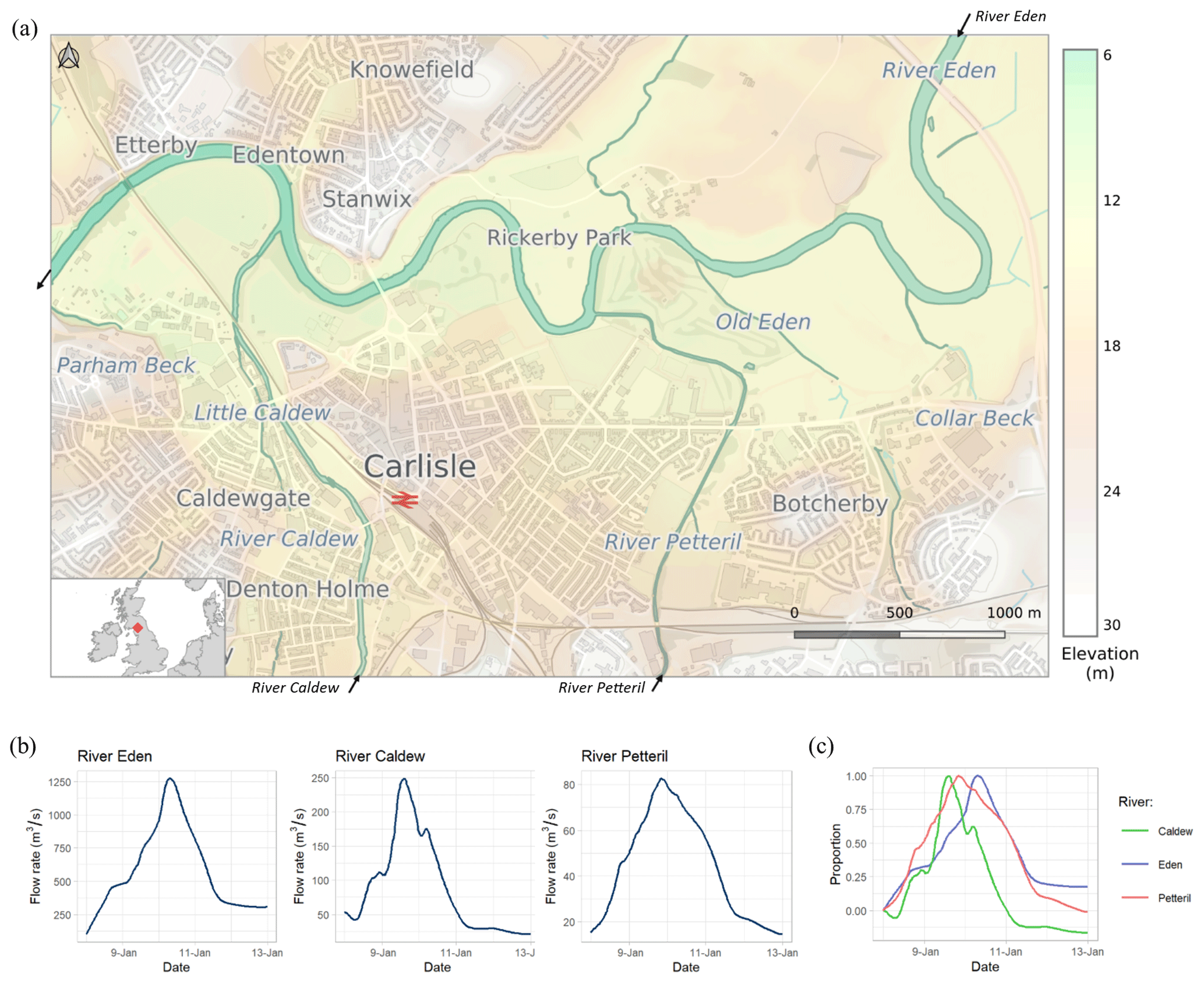
Figure 4 (a) Study site 1 at Carlisle, UK, at the confluence of the rivers Caldew, Petteril, and Eden, showing elevation from lidar. The plots in panel (b) show river flows for the January 2005 flood event simulated. The plot in panel (c) shows the relative level of the three rivers (calculated as a proportion of the difference between the flow on 8 January and the flood peak) and indicates that the River Caldew reached the flood peak ∼5.5 h ahead of the River Petteril and ∼17 h ahead of the River Eden. This figure contains OS data © Crown copyright and database right (2020).

A simulation was run using a model grid of 5 m (domain size of 951×612 cells; 14.6 km²), topography from lidar (Environment Agency, 2020), and inflows from gauging station records (Environment Agency, 2021). The simulation began on 8 January 2005, 00:00 UTC for 120 h (5 d). Visualisations of the model output are shown in Fig. 5. Flood water mixing is shown in the RGB colour space, using Eq. (15) to enable darker shades to indicate deeper water. The mixing of Eden (blue) and Petteril (red) gives pink shades, which, as it moves downstream, transitions towards purple due to the larger volume of flow on the Eden. Water from the Caldew is shaded in green and contributes to the greyer shades in the floodplains close to the main channel as the three waters are mixed.

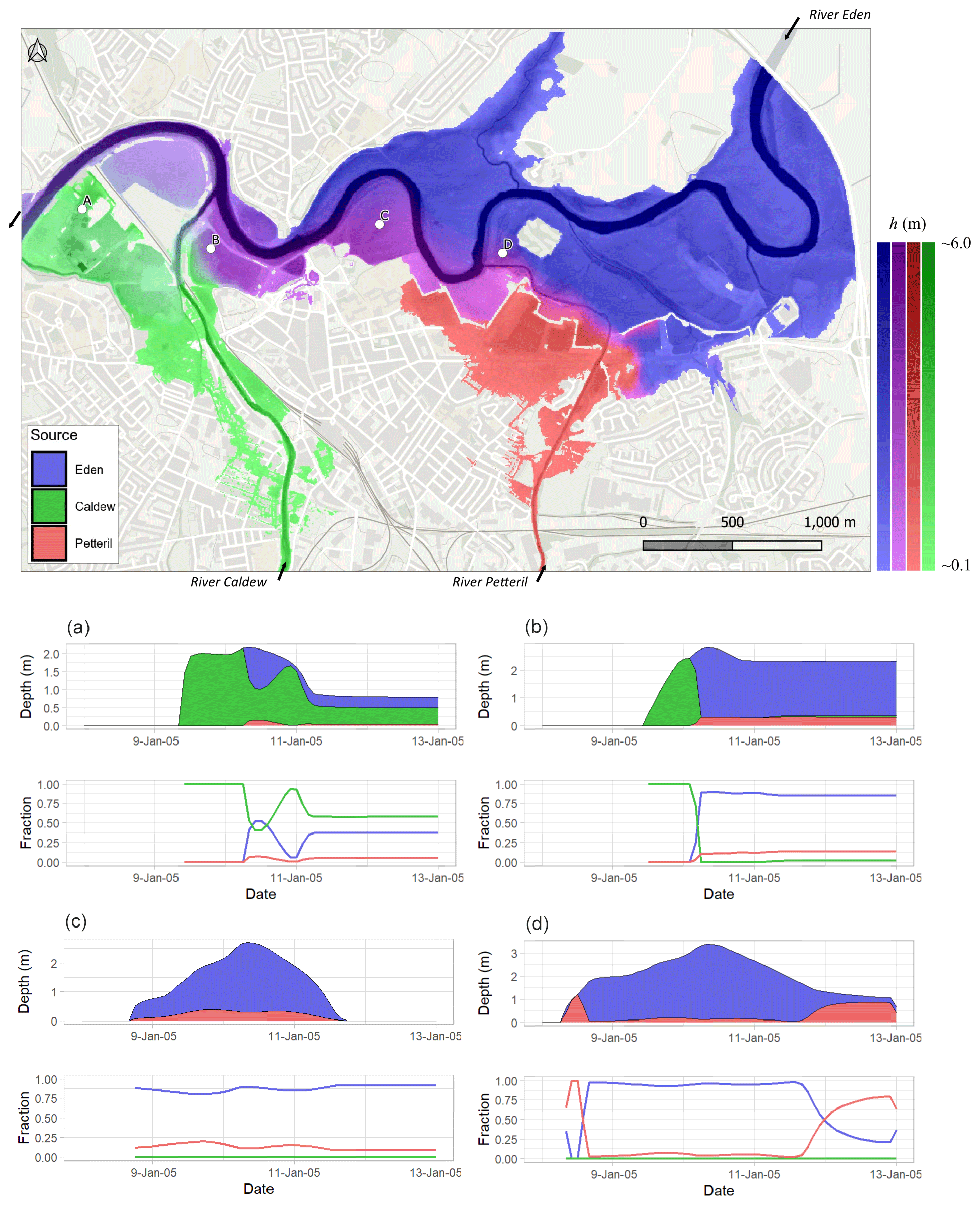
Figure 5 Model results for Carlisle, showing the flood extent on 10 January 2005, 06:00, close to the flood peak. Map colours indicate the mixing of water from different sources, with darker shades indicating increased depth. Colour scales show depths with selected source combinations (left to right), namely ϕ _[Eden]=1.0 (blues), ϕ _[Eden]=0.8, ϕ _[Petteril]=0.2 (pinks/purples), ϕ _[Petteril]=1.0 (reds), and ϕ _[Caldew]=1.0 (greens). β = 0.2 is used to emphasise lower water fractions from the Caldew and Petteril rivers. Depths and fractions for four selected locations, marked A–D, are shown. This figure contains OS data © Crown copyright and database right (2020). For an animated version, please see https://youtu.be/xOtOi06cXvA (last access: 25 April 2023) or the video supplement provided.

The ability to trace inputs from discrete tributaries allows us to determine how differently sourced flood waters contributed to the flooding. This is especially pertinent to the Carlisle 2005 flood events, where the most flood damage was considered to have come from the two tributary inputs, namely the Caldew and Petteril (Environment Agency, 2006). For example, the time series plots in Fig. 5 illustrate the locations where water is mixed from multiple sources. The larger volume of water from the River Eden dominates, but at point A, a railway embankment prevents flooding from the Eden, but the area is flooded by the Caldew. Points B and D are initially flooded by the Caldew and Petteril, respectively, until flooding from the Eden arrives. This is likely due to the timing of the flood peaks (∼11.5 h earlier on the Petteril than the Eden; ∼17 h earlier on the Caldew).

3.2 Avon–Heathcote estuary, Christchurch, New Zealand

On the eastern edge of the city of Christchurch, New Zealand, the estuary of the Avon and Heathcote rivers (Fig. 6) is a large (∼8 km²), shallow (mean depth ∼1.4 m at spring high tide and a tidal range of ∼1.7–2.2 m) intertidal area, with about 85 % of its elevation above the spring low tide level (Findlay and Kirk, 1988). The estuary is semi-enclosed and separated from the Pacific Ocean by a ∼4.5 km long spit (the Christchurch suburbs of New Brighton and/or Southshore. It has been designated as a site of ecological significance in the Christchurch District Plan (Christchurch City Council, 2016) and is internationally recognised for its importance as a habitat for migratory bird species (Woodley, 2018). The estuary acts as a sediment trap for inflows from the Avon and Heathcote rivers, the catchments of which cover a combined area of 188 km², which is largely urbanised, meaning that urban pollution is a considerable issue (Vopel et al., 2012).

Here, we demonstrate water source tracing and visualisation for the Avon–Heathcote estuary for the month of July 2017, using a model grid of 10 m (domain size of 483×675 cells; 32.6 km²), derived from lidar (Land Information New Zealand, 2015). The sources of water included were the two rivers, with inflow from the Avon River from the north and inflow from the Heathcote from the southwest (Environment Canterbury, 2023) and a downstream tide boundary condition at the estuary outlet at the southeast (Fig. 6b). The simulated period of July 2017 included both the neap and spring tides and a high-flow event on 22 July on both rivers, where the Avon River peaked at 13:00 with 14.7 m³ s⁻¹ of flow, close to the mean annual flood level (Environment Canterbury, 2023), and Heathcote River peaked at 14:00 with 28.1 m³ s⁻¹ of flow, which is an annual exceedance probability of less than 0.1 (Environment Canterbury, 2023).

As noted in Sect. 2.3, as a depth-averaged model, CAESAR-Lisflood does not account for the higher density of the saline tidal water compared to fresh riverine water, meaning that variations of any kind in the vertical salinity profile of estuarine water are not accounted for. However, given that the Avon–Heathcote estuary receives only small volumes of riverine inflow, with mean inflow from the Avon and Heathcote rivers of 1.87 and 1.04 m³ s⁻¹, respectively (LAWA, 2023), compared with tidal inflow rates of up to 500–800 m³ s⁻¹ during an incoming tide (van der Peet and Measures, 2015), it is likely that it is well mixed, with little vertical salinity difference (Hansen and Rattray, 1966).

The results of the model application are shown in Fig. 7. During low-flow conditions during at low tide on 8 July 2017 (image A), the estuary is mostly drained, with the water remaining in the estuary containing a greater proportion of water from the Avon River as a result of its higher baseflow. Shortly after the spring high tide on 16 July (image B), it can be seen that water from both the Avon and Heathcote is pushed back by the tide, particularly along the eastern shoreline. If accurate, this situation may play a significant role in determining where pollutants, such as those from storm water runoff, which are then discharged from the Avon and Heathcote rivers (e.g. see Vopel et al., 2012), are deposited. This would affect human health through various activities in the estuary, such as the gathering of food sources such as fish and shellfish which accumulate heavy metals contained in riverine discharge (e.g. McMurtrie, 2015).

During the high-flow conditions on 22 July, shortly after the high tide and inflow peak (image C) and low tide (image D), the results indicate a substantially greater riverine contribution to the estuary, such that, after the fall of the tide, the estuary remained substantially inundated but with almost all water being from riverine sources. After high tide, the Avon and Heathcote waters are largely confined by the tide to the western shore, with a clear boundary between the two river sources being visible. After low tide, this boundary is sharper, due to the absence of tidal mixing, and gradually dissipates as water mixes towards the estuary outlet.

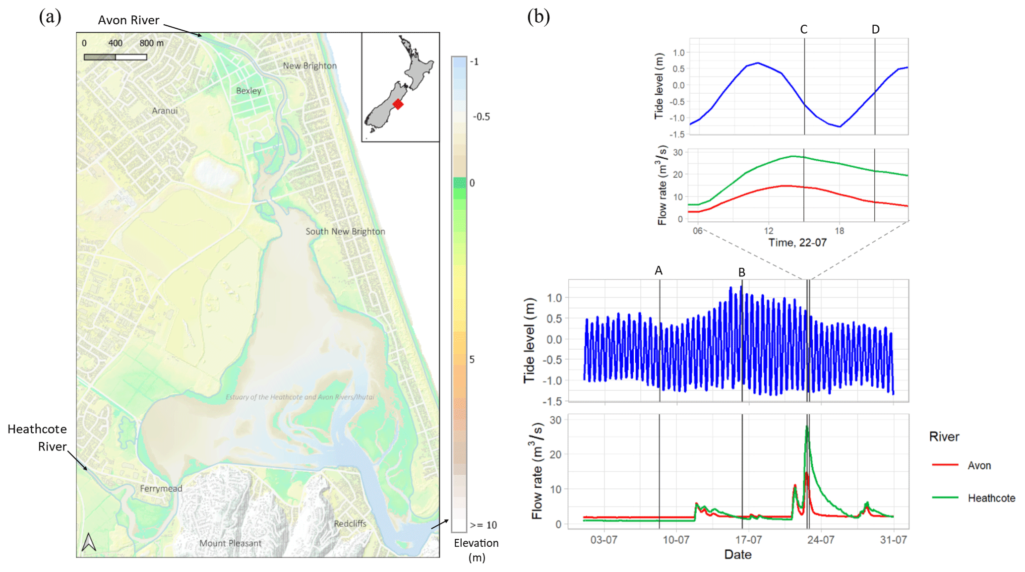
Figure 6 (a) Study site 2 at the Avon–Heathcote estuary in Christchurch, New Zealand, showing elevation from lidar. (b) Inflow and downstream tide levels for the period simulated in July 2017, which includes a high-flow event on 22 July. The four vertical lines labelled A–D represent the timing of the images shown in Fig. 7. Tide data are from the National Institute for Water and Atmospheric Research (NIWA) Sumner Head gauge, which is around 1 km from the estuary outlet. Flow data are from the Environment Canterbury gauges at Gloucester Street (Avon) and Buxton Terrace (Heathcote). This figure contains data sourced from the Land Information New Zealand (LINZ) Data Service and is licensed for reuse under CC BY 4.0.

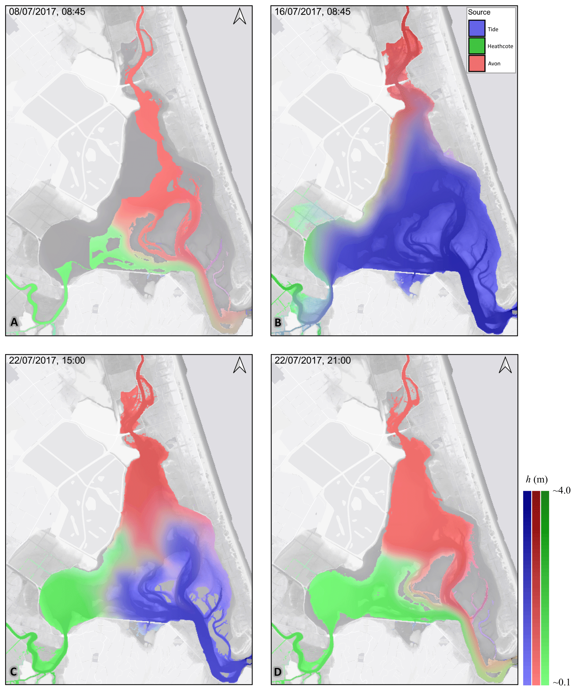
Figure 7 Model results for the Avon–Heathcote estuary. Low-flow conditions are shown during (a) low tide on 8 July 2017 and (b) after the spring high tide on 16 July. High-flow conditions are shown on 22 July shortly after high tide (c) and low tide (d). The images were produced with β=0.2. Their timing and flow and/or tide levels are shown in Fig. 6. Map colours indicate the mixing of water from different sources, with darker shades reflecting increased depth. The colour scales show depths for individual sources (left to right), namely ϕ _[Tide]=1.0 (blues), ϕ _[Avon]=1.0 (reds), and ϕ _[Heathcote]=1.0 (greens). The background images contain NationalMap Basemaps (CC-BY-ND license) and lidar data shaded in grey. For an animated version, please see https://youtu.be/Fczr5tczzXU (last access: 25 April 2023) or the video supplement provided.

3.3 Amazon River, Brazil

The flow of the central Amazon River is characterised by a large annual flood wave of around 10 m amplitude, resulting primarily from the distinctive wet and dry seasons (Trigg et al., 2009). Each year, during the wet season, the Amazon rises and inundates its low-lying floodplain forests, creating an internationally significant wetland ecosystem which reaches its maximum extent in around June or July (Mitsch and Gosselink, 2015), with the extensive surface water flow recognised as being a key factor in the functioning of the habitats created and exerting a strong control on biological and biogeochemical processes (Richey et al., 2002; Wittmann et al., 2004). The inter-annual variability in the flood level and flood wave timings creates spatial and temporal complexities on the floodplain (Melack and Hess, 2011), with the source of the water being recognised as a key determinant for sediment transport (Vauchel et al., 2017) and trace element concentration (Baronas et al., 2017) dynamics across the basin.

We applied the model of Wilson et al. (2007) to a ∼ 300 km reach of the Solimões River (Amazon River mainstem) at its confluence with the Purus River (Fig. 8), using a model grid of ∼278 m (domain size of 966×479 cells; ∼ 35 650 km²) for the period of October 2013 through December 2014. Operating at a far larger spatial scale compared to examples 1 and 2, here water source tracing results show that, downstream (west) of the river confluence, the southern floodplain is primarily inundated with water from the River Purus (indicated by green), while the floodplain to the north contains a mix of water from the rivers Solimões and Purus (indicated by orange; Fig. 9). The shared floodplain upstream of the confluence displays a clear gradient transition between the two water sources, passing from red (Solimões), through yellow (equal mix), and to green (Purus). The cross-sectional profile plots in Fig. 9 show that, after flowing into the Solimões, water from the Purus remains largely on the right (southern) bank but mixes with the water from the Solimões as the river progresses downstream. As the Purus peaks sooner than the Solimões, the proportion of water from the Purus close to the right bank decreases through the Solimões flood peak (C) and mid-falling water (D). These demonstrate the ability of the LISFLOOD-FP and the new tracing functions to simulate the convergence and mixing of water from these two major river systems. The proposed water source tracing method therefore provides the means to assess the complex dynamics of variable contributions in river–floodplain systems, such as those on the Amazon, enabling the estimation of important variables which are associated with each water source through time, such as nutrient availability. Furthermore, it may enable a rapid assessment of issues of importance for human health, such as identifying areas which may be susceptible to mercury contamination from gold mining activities in the Amazon basin, for which the dynamics of fluvial and pluvial waters are key factors (Maurice-Bourgoin et al., 2003; Maia et al., 2009). However, for a robust analysis, it is likely that additional tracing of sediment erosion, transportation, and deposition is required (e.g. Haddadchi et al., 2019).

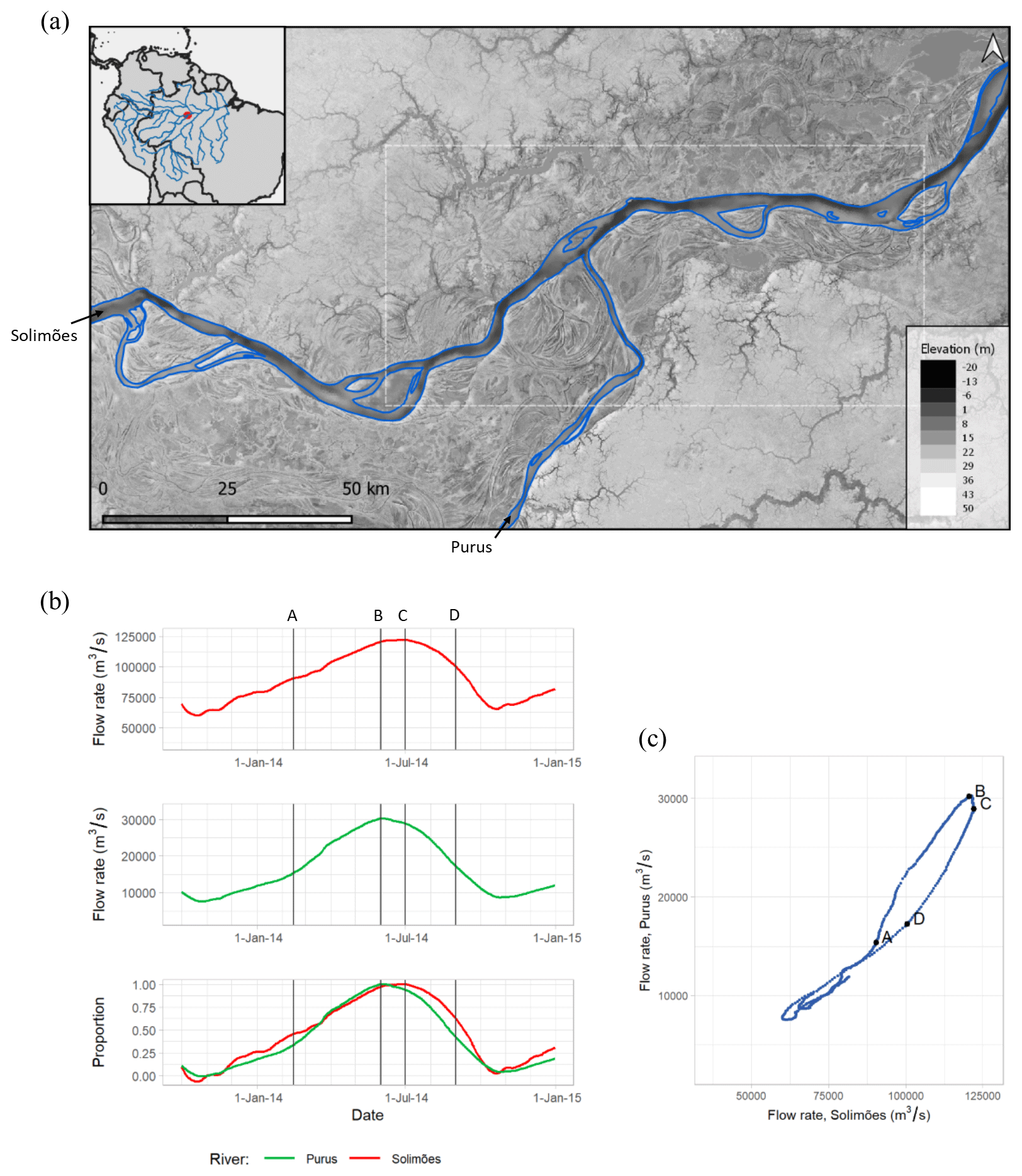
Figure 8 (a) Study site 3 at the confluence of the Solimões (Amazon River mainstem ) and Purus rivers in the central Amazon, Brazil, showing elevation derived from SRTM (Shuttle Radar Topography Mission; O'Loughlin et al., 2016) and bathymetry (Wilson et al., 2007). The plots in panels (b) and (c) show river flows for the period simulated from October 2013 through December 2014 (Agência Nacional de Águas e Saneamento Básico, 2023). The lower plot of panel (b), which shows the relative level of Solimões and Purus flow (calculated as a proportion of the difference between the flow on 1 November 2013 and the 2014 peak flow), indicates that the Solimões rises more steadily and before Purus, which has a later, steep rise from around mid-February onwards. Peak flow levels on Purus (indicated by letter B) occurred around 1 month earlier than the peak flow on Solimões. The dotted box in panel (a) and letters A–D in panels (b) and (c) indicate the location and timing of the model results shown in Fig. 9. This figure contains Natural Earth data in the public domain.

Figure 9 Model results for the Amazon, with colours on the map at Purus flood peak (top) indicating the mixing of the waters along the channel and across the floodplain. Map colours indicate the mixing of water from each source, with darker shades reflecting increased depth. Colour scales show depths with selected source combinations (left to right), namely ϕ _[Solimões]=1.0 (reds), ϕ _[Purus]=1.0 (greens), and ϕ _[Solimões]=0.75, ϕ _[Purus]=0.25 (yellows). Channel cross-sectional plots (bottom) at locations indicated by a–a^′ and b–b^′ show the water source fractions (upper plots) for each channel (A = mid-rising; B = Purus flood peak; C = Solimões flood peak; D = mid-falling) and depth/source profiles (lower plots) for image B (Purus flood peak). For an animated version, please see https://youtu.be/PknAL_8fd1I (last access: 25 April 2023) or the video supplement provided.

3.4 Computational performance

The results of the planar test case are shown in Fig. 3b–d. Flow depth at t=8400 s is shown in Fig. 3b, and a water source visualisation at the same time for the simulation with all eight sources is shown in Fig. 3c. Here, flood water mixing is shown in the RGB colour space, as per Eq. (14) (i.e. in which the mixing of sources 2 (red) and 4 (green) gives yellow and the mixing of sources 4 and 6 (blue) gives cyan). Other water sources are shown in black. As the water flows down the slope, it becomes increasingly mixed within each section and is helped by water being forced to flow through the gaps left in the walls placed across the slope. Once the water flow reaches the bottom of the slope, a high proportion of the domain contains water (77 901 out of 80 000 cells). The flow is constrained to flow out of the domain through eight gaps in the downstream boundary wall (marked A–H in Fig. 3a). The fractions of water sources 1–8, at locations A–H, throughout the simulation are shown in Fig. 3d. As the domain has mirror symmetry along the west–east axis at y=500 m, the fractions at each of the locations are also symmetrical with respect to water sources. For example, at location A, water from source 1 increases to a fraction of around 0.5 of the water flowing through this location at steady state, while water from source 8 does not reach it at all; the reverse is true for these water sources at location H. For the two central locations, D and E, all water sources are present, with steady-state fractions ranging from around 0.02 (for source 8 at location D or source 1 at location E) to 0.2 (for sources 4 and 5).

Code profiling, using the diagnostic tools of the Microsoft^® Visual Studio 2019 compiler software (version 16.11.2), based on this test application with three sources, indicates that update_tracer_states() uses around 17.9 % of the CPU resources allocated to CAESAR-Lisflood during a simulation, with 3.0 % used for save_tracer_states(). This compares to 39.6 % for qroute() and 11.5 % for depth_update(). This profiling was completed on a Microsoft^® Windows^® 10 (build 18363) computer system with an Intel^® Xeon^® E-2278G CPU running at 3.4 GHz base (5.0 GHz maximum turbo) frequency with 8 cores or 16 threads, with 128 Gb of system memory (4×32 Gb Samsung M391A4G43MB1-CTD ECC RAM UDIMM running at 2666 Mbps), writing outputs to a Samsung NVMe™ Solid State Disk (SSD; MZVLB1T0). All simulations presented in this paper were completed on this computer system.

Table 2 Summary of the simulations completed for each of the three study sites presented and their computational costs.

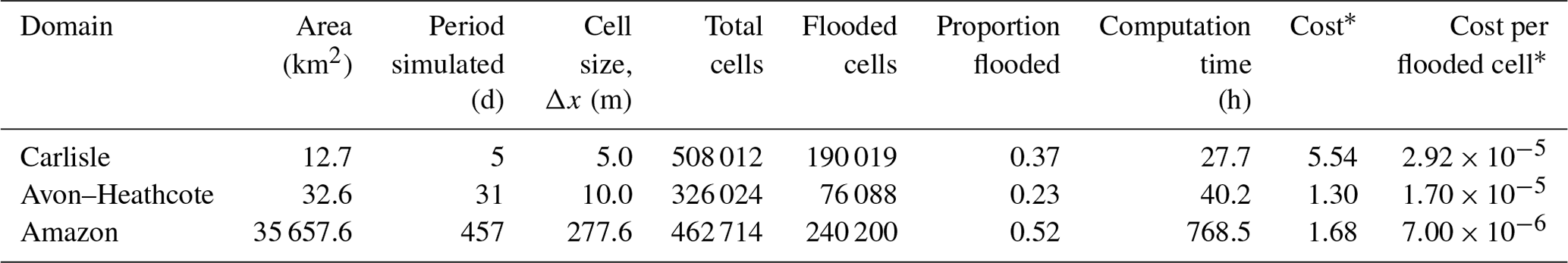
^* Number of computation hours needed per day of the period simulated.

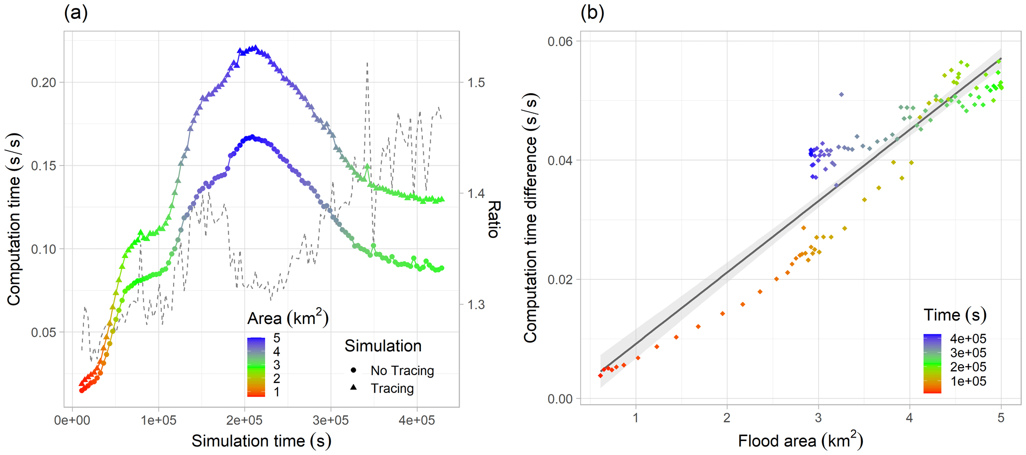
Figure 10 Computational efficiency of water source tracing for the Carlisle simulations with and without water source tracing. (a) Computation time required per second of the 5 d (432 000 s) simulation, with colours indicating the area of inundation; the dashed line shows the ratio between the two (secondary y axis). (b) Computation time difference (i.e. cost of tracing) against flood area, with a linear model fitted for reference; colours indicate the simulation time.

The total time of each of the eight simulations is presented in Table 1, ranging from 1362.5 s with two tracers up to 1925.2 s with eight tracers, as compared to 800.6 s without water source tracing. The ratio of the computation time for the full simulations with tracing, against computation time without tracing, ranges from 1.7 for two sources to 2.4 for eight. The mean computational requirement time ranged from 0.016 s s⁻¹ for two tracers to 0.022 s s⁻¹ with eight tracers, compared to 0.009 s s⁻¹ without water source tracing. In addition, the variability in the computational costs increases with the number of sources being traced, likely due to the complexity of the mixing introduced by constraining flow through gaps within this test case.

Table 2 summarises each of the domains and simulations completed for the Carlisle, Avon–Heathcote, and Amazon study sites. Although the computational cost for the Amazon simulation was highest (∼32 d of computation time), when normalising for the larger number of flooded cells and the longer simulation period, it had the lowest computational cost. This higher computational efficiency likely results from the longer model time step used, due to the larger cell size (Δx=277.6 m). For the Avon–Heathcote domain (Δx=10 m), the computational cost per flooded cell per day of period simulated was 2.4 times the cost for Amazon; for the Carlisle domain (Δx=5 m), this ratio increased to 4.2.

Figure 10 illustrates the computational efficiency of our scheme for the Carlisle flood model, with and without water source tracing. Computational requirements for the simulation with water source tracing were found to be between 1.2× and 1.5× the simulation without tracing, which is less than the 1.8 ratio found for the planar test case with three water sources. As with the planar test case, the computational requirements of water source tracing were found to increase with the area of inundation. Early in the simulation, when the flood area was around 1 km² (40 000 cells), the computational overhead of water source tracing was approximately 0.01 s s⁻¹. This increased nearly linearly to ∼0.05 s s⁻¹, as the flood extent reached its peak extent of around 5 km² (200 000 cells).

4 Discussion

Our method for water tracing is simple, effective, and has a low additional computational overhead of 1.2–1.5 for our real-world test cases. The three case studies above show that the approach is flexible and applicable in urban, coastal, and fluvial environments over a wide range of spatial scales. An important advantage of the method is that the number of water sources which may be traced is limited only by computational constraints. Furthermore, as the formulation records the proportion of different tracers or water sources per cell, it is fully independent of the hydraulic calculations, meaning it is straightforward to add to existing finite-volume codes and similar 2D flow models to LISFLOOD-FP. This also means that the predicted water levels with or without the tracers are identical.

However, it is important to remember that the speed and simplicity of the method is at the expense of treating cell water volumes as being fully mixed. This means that it is possible for small fractions of a tracer or water from different sources to propagate quickly downstream, since fluxes into a cell would be included for all of the fractions assigned as an inflow to a downstream neighbouring cell. In effect, this represents a tiny amount of the numerical diffusion, and the volumes moved are very small, but as a result, caution should be applied to the interpretation of very small water source fractions. This is also an issue for tracing functions in other codes such as TELEMAC (e.g. chap. 9.5 Ata et al., 2014). Additionally, as each cell is treated as fully mixed, we cannot yet incorporate the effects of different water densities, such as saline water.

These issues notwithstanding, this method provides excellent opportunities for the simplified simulation of water, solute, and waterborne fluxes across river catchments and in estuaries. In particular, with the CAESAR-Lisflood implementation combining a hydrological and hydraulic model, the contributing effects of subbasins on flooding can easily be simulated. Furthermore, the ability to combine both point source (e.g. from combined sewer outflows) and diffuse source (e.g. fields) contaminants within a computationally fast model opens up many opportunities to simulate water quality and pathogen and/or contaminant issues. Assessments of water sources may be especially useful for other fluvial or estuarine sites with similar human health considerations to the examples presented here. For example, Robins et al. (2019) assessed water quality risks from viral dispersal from the Conwy catchment, north Wales, and highlighted the importance of river flow contributions to exposure risk. Therefore, this simple and efficient water tracing algorithm within the open-source CAESAR-Lisflood model provides a powerful tool for studying the effect of water quality and contaminant issues on environmental and human health.

5 Conclusions

We developed a simple method for tracing water sources through a flood inundation model and demonstrated its application for a simple test case and three example case studies at different spatial and temporal scales. A key advantage of the approach lies in its independence from the hydraulic methodology used, meaning that it is relatively straightforward to add to existing in finite-volume codes. The method enables an effective and informative visualisation of flood inundation, providing additional insight into flood dynamics. In addition, it may potentially provide the ability to simulate the movement of solute contaminants and pathogens within a computationally efficient model, although additional testing is required to verify the reliability of the method, given the assumption of full mixing within cells.

Appendix A: Code description

The tracing component requires a series of additional variables representing the water state prior to the routing (Fig. A1). The variable water_depth_prev is an array of X×Y grid cells containing the depth from the previous time step. dhdt_x and dhdt_y are arrays containing the change in cell depth in the last time step in for columns and rows, respectively. The fraction of each cell from each source (i.e. the water tracers) are recorded in a series of three-dimensional ($W\times X\times Y$ grid cells) or stacked arrays containing the tracer fractions per cell for present and previous iterations (watertracer, watertracer_prev) the rain zonations (watertracerRainZone, watertracerRainZone_prev), and a series of flags to enable or disable tracing. Note that the rainfall source as a whole (i.e. from any zone) is contained within the main watertracer arrays, while the fraction of rainfall from each zone is recorded in the watertracerRainZone arrays.

The addition to the reach inputs is shown in Fig. A2, from the function reach_water_and_sediment_input() (rainfall inputs and tidal or stage inputs are added similarly, but the code is omitted for brevity). In this function, the updated water source fractions for the water source being added to the cell (Eq. 9) and other sources already in the cell (Eq. 10) are implemented on lines 33 and 40, respectively.

After the addition of boundary condition inputs from each source, the new tracer states (prior to surface water routing) are saved within the function save_tracer_states(), in which the waterdepth, watertracer, and watertracerRainZone arrays are copied into the waterdepth_prev, watertracer_prev, and watertracerRainZone_prev arrays, respectively (Fig. A3).

Flow rates between all cells are then calculated as normal in the function qroute() (i.e. solving Eq. 2 between all cells), with no modifications needed to the code for water source tracing. Once flows are calculated, depths are updated according to Eq. (1) in the function depth_update(). Here, the only modification required for water source tracing is that the volumes of water moving between cells is recorded in the dhdt_x and dhdt_y arrays (Fig. A4). Here, the dhdt_x and dhdt_y arrays are updated on lines 18–24, before the water_depth array is updated according to Eq. (1) on line 27. For brevity, the code presented in Fig. A4 omits some additional processing for updates to suspended sediment and error checking.

Finally, the main addition to the CAESAR Lisflood code for water source tracing is within the function update_tracer_states() that deals with the mixing component and updates the different source tracer fractions as water is moved between cells during each iteration (Fig. A5). In the update_tracer_states() code, the cell depth after the removal of outflows, $h_{Q_{\left[\text{out}\right]}}^t$ (Eq. 7), is first calculated (lines 31–43). Then, the updated volume fractions (Eq. 6) obtained for each source are calculated (lines 45–81), with the total volume contributed from each source first calculated (lines 47–58), and then the updated cell volume fractions are obtained (lines 77–79). Finally, the function will update the volume fractions for each rainfall zone source in a similar way (code omitted for brevity).

Figure A1 Additional variables required for water source tracing.

Figure A2 Updating cell water fractions according to Eqs. (9) and (10) from the function reach_water_and_sediment_input().

Figure A3 The function save_tracer_states().

Figure A4 Modified depth_update() function.

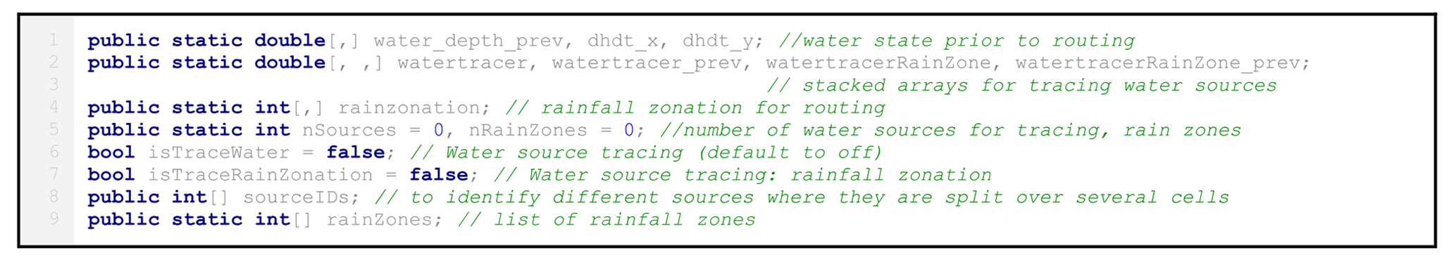
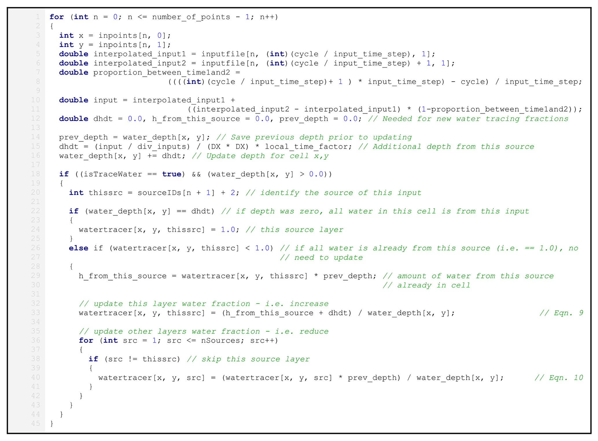
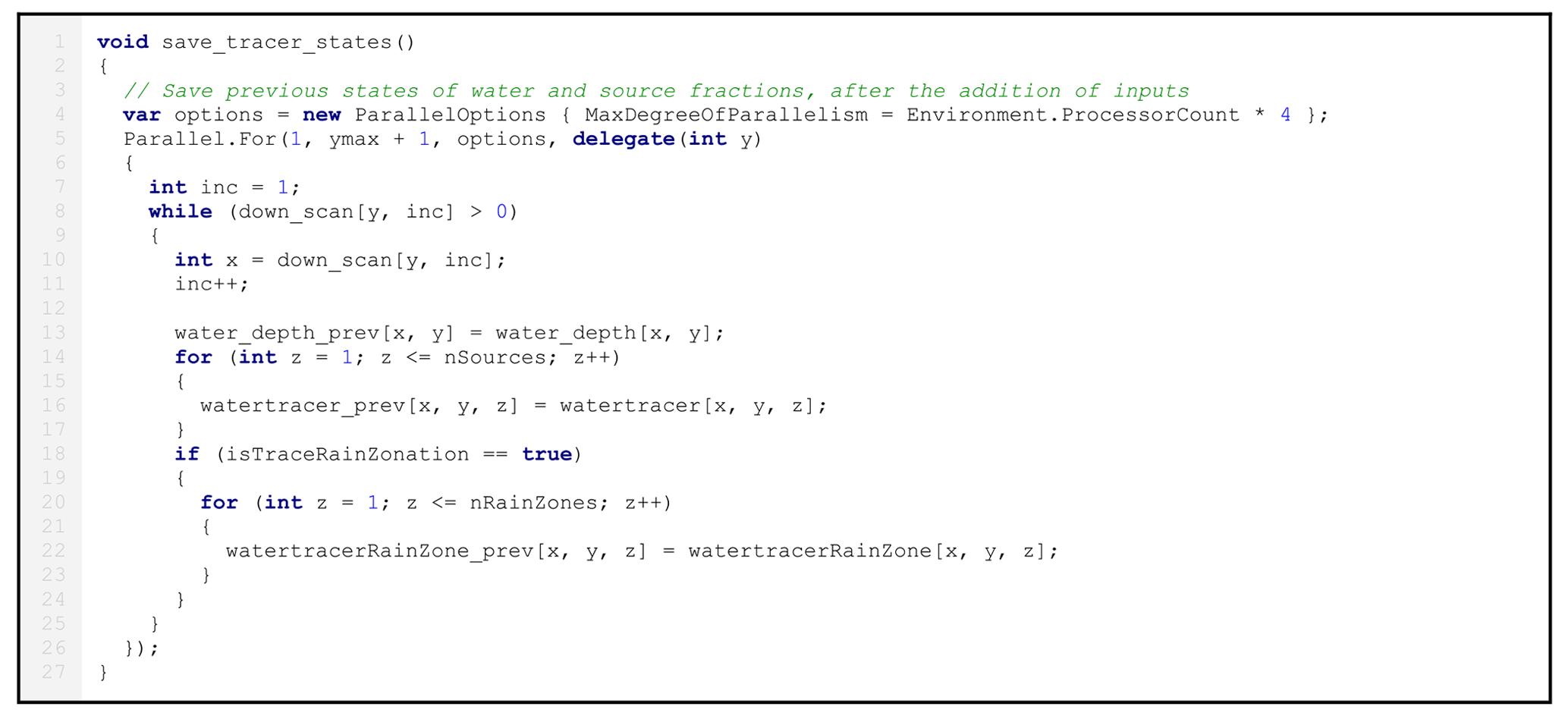
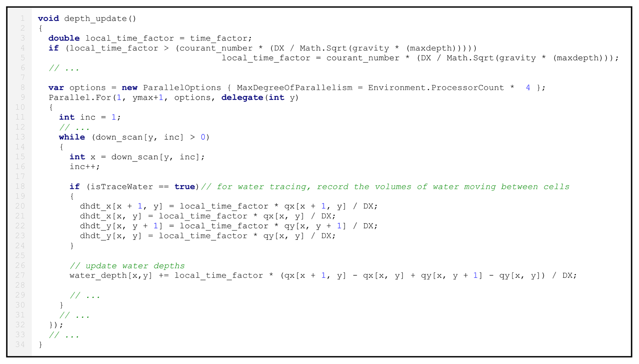
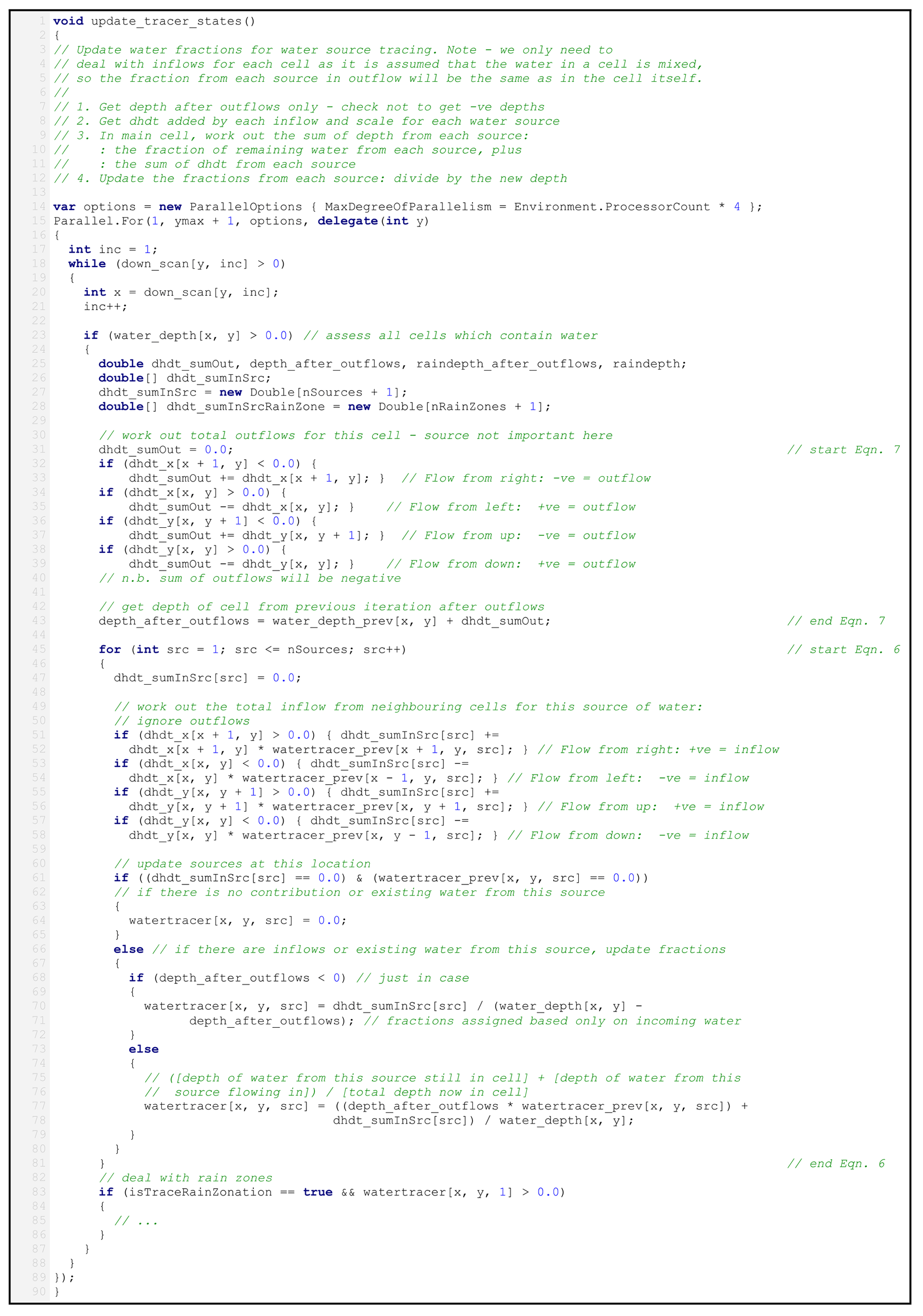
Figure A5 The main water source tracing calculations within the update_tracer_states() function.