Accelerating models for multiphase chemical kinetics through machine learning with polynomial chaos expansion and neural networks

The heterogeneous chemistry of atmospheric aerosols involves multiphase chemical kinetics that can be described by kinetic multi-layer models (KMs) that explicitly resolve mass transport and chemical reactions. However, KMs are computationally too expensive to be used as sub-modules in large-scale atmospheric models, and the computational costs also limit their utility in inverse-modeling approaches commonly used to infer aerosol kinetic parameters from laboratory studies. In this study, we show how machine learning methods can generate inexpensive surrogate models for the kinetic multi-layer model of aerosol surface and bulk chemistry (KM-SUB) to predict reaction times in multiphase chemical systems. We apply and compare two common and openly available methods for the generation of surrogate models, polynomial chaos expansion (PCE) with UQLab and neural networks (NNs) through the Python package Keras. We show that the PCE method is well suited to determining global sensitivity indices of the KMs, and we demonstrate how inverse-modeling applications can be enabled or accelerated with NN-suggested sampling. These qualities make them suitable supporting tools for laboratory work in the interpretation of data and the design of future experiments. Overall, the KM surrogate models investigated in this study are fast, accurate, and robust, which suggests their applicability as sub-modules in large-scale atmospheric models.

1 Introduction

An accurate description of the heterogeneous chemistry of atmospheric particles requires explicit coupling of mass transport with chemical reactions (Pöschl et al., 2007; Kolb et al., 2010; Shiraiwa et al., 2014). Especially for particles containing secondary organic matter, field and laboratory experiments during the last decade showed severe transport limitations that affect chemical reactivity (Shiraiwa et al., 2011; Kuwata and Martin, 2012; Berkemeier et al., 2016). While the elementary processes are well understood, kinetic multi-layer models (KMs) describing mass transport and chemical reactions at the gas–particle interface and throughout the particle bulk are computationally expensive due to the need for spatial resolution within the particles (Pöschl et al., 2007; Shiraiwa et al., 2012; Roldin et al., 2014; Berkemeier et al., 2017; Semeniuk and Dastoor, 2020; Dou et al., 2021). For use in global or regional models, the KMs would have to be evaluated for every grid cell, time step, and particle class (size and composition). This computational volume makes the application of KM extremely costly, if not outright impossible.

A second complicating factor for KMs is the multitude of chemical and physical input parameters, such as transport parameters or chemical reaction rate coefficients, which are often poorly constrained or unknown. Thus, in a laboratory setting, KMs are often used in an inverse-modeling approach, in which model parameters are deduced or constrained with experimental data using global optimization (Berkemeier et al., 2017; Tikkanen et al., 2019; Berkemeier et al., 2021; Wei et al., 2021; Milsom et al., 2022). However, due to the inherently coupled nature of the underlying physical and chemical processes, input parameters are often ill constrained; i.e., their numerical value cannot be uniquely determined (Berkemeier et al., 2017). This is particularly problematic when extrapolating the KMs to conditions outside the calibration range, where the calculation outcome can depend strongly on previously insensitive and thus unconstrained parameters (or combinations of parameters). Fit ensembles, i.e., arrays of multiple solutions from repeated execution of a global optimization algorithm, can be utilized to propagate the uncertainty of the global fit to conditions outside the calibration range (Berkemeier et al., 2021). Solving the inverse problem is a complex task that becomes computationally more expensive with an increasing number of uncertain model input parameters, often requiring >10⁵ model simulations (Xu et al., 2018). In some cases, this can be prohibitively expensive to do with a full model, and the problem is exacerbated when acquiring or evaluating fit ensembles.

Computationally inexpensive surrogate models can replace KMs in specialized tasks and help solve the issue of computational cost. These surrogate models are trained on a dataset consisting of a wide range of kinetic input parameters and the associated calculated outputs until they reproduce the KM output with the desired accuracy. Surrogate-based optimization methods are an active field of research (Booker et al., 1999; Vu et al., 2017; Xu et al., 2018). Some studies use an iterative approach, wherein the surrogate model is used to constrain the likely parameter space, and the full model is run within this likely parameter space to refine the surrogate model. Here, we illustrate the generation of surrogate models by introducing two suitable machine learning methods, namely artificial neural networks (NNs) through the Python package Keras (Gulli and Pal, 2017) and polynomial chaos expansion (PCE) with UQLab (Marelli and Sudret, 2014).

Artificial NNs represent a group of common machine learning algorithms. Their functionality is inspired by biological brains, where complex computational processes are based on comparably simple interactions of large numbers of interconnected nodes or neurons (Kröse and van der Smagt, 1996). Neural networks are commonly organized in layers, where an individual neuron obtains signals from neurons in the previous layer and maps them to a single new signal that is passed to neurons of the following layer (Almeida, 2001; Popescu et al., 2009). By systematic variation of the numerical weights of individual neuron operations, the so-called training, an NN can increase its predictive accuracy. The exact mathematical operations that are performed by neurons in specific layers and the arrangement of such layers (architecture of the NN) are determined by so-called hyperparameters. Hyperparameters can be adapted to obtain an NN that is specialized for a specific task, input data structure, or output type (Bishop, 1994; Sadeeq and Abdulazeez, 2020).

In the atmospheric sciences, NNs are used for air quality prediction, function approximation, and pattern recognition tasks (Gardner and Dorling, 1998), but their application as surrogate models for computationally expensive KMs is less well researched. Recently, popular applications of machine learning in atmospheric chemistry and physics include quantitative structure–activity relationship (QSAR) models that map molecular structures to compound properties as an alternative to time-consuming laboratory experiments or quantum mechanical calculations (Lu et al., 2021; Lumiaro et al., 2021; Galeazzo and Shiraiwa, 2022; Krüger et al., 2022; Xia et al., 2022). Holeňa et al. (2010) used surrogate models in computationally costly evolutionary optimization and successfully enhanced this approach with the application of NNs. Tripathy and Bilionis (2018) used an NN to create surrogate models for expensive high-dimensional uncertainty quantification. Other recent applications of NNs as surrogate models address chemical and process engineering (Cavalcanti et al., 2021; Esche et al., 2022) or materials science (Allotey et al., 2021). Machine-learning-based surrogate models have also found application as modules in geoscientific models, including large-scale atmospheric chemistry, transport, and climate models, to reduce computational cost in very demanding tasks such as atmospheric convection (O'Gorman and Dwyer, 2018), gas-phase and heterogeneous chemistry (Keller and Evans, 2019; Kelp et al., 2020; Sturm and Wexler, 2022), or aerosol and cloud microphysics (Rasp et al., 2018; Harder et al., 2022). These surrogate models function either as parameterizations for subgrid processes or replace the chemical integrator.

The second method applied in this work is polynomial chaos expansion (PCE), a method commonly used for uncertainty quantification (Sudret, 2008). In the PCE approach, the full model is represented as a series of suitably built, multivariate, and orthonormal polynomial functions (Marelli and Sudret, 2014). Surrogate models using PCE methods have been developed mainly within engineering fields (Ghanem and Spanos, 2003; Sudret, 2008). Several recent environmental chemistry investigations have applied PCE surrogate modeling, particularly because of its suitability for global sensitivity analysis problems (Thackray et al., 2015; Feinberg et al., 2020). The goal of global sensitivity analysis is to apportion the uncertainty in model output into contributions from the uncertainties of different model input variables, additionally considering interacting effects between input parameter uncertainties (Saltelli et al., 2008). The results from the sensitivity analysis indicate which are the most influential input parameters that should be further constrained and may therefore be a useful tool in designing or prioritizing laboratory experiments.

2 Methods

The surrogate-modeling workflow employed in this study is shown in Fig. 1. To acquire a fast-computing surrogate model for the computationally expensive KMs, training data are first acquired by sampling outputs of the full model from the possible model parameter space. The surrogate models are trained with Keras and UQLab on this data and are validated by comparison with a test dataset of full model output.

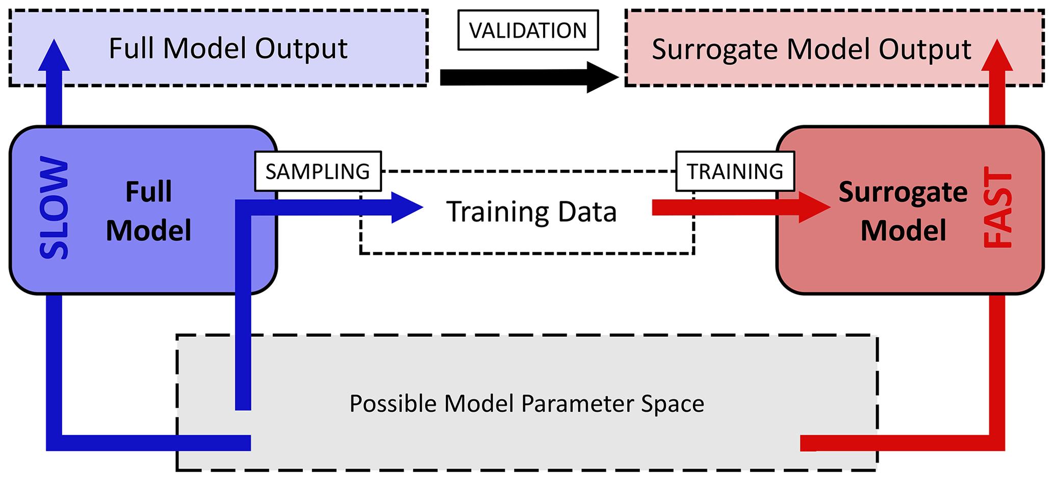
Figure 1 Workflow chart for the surrogate-modeling process employed in this study. The possible or desired model parameter space (gray) is sampled with the slow-computing full model (blue) to acquire training data consisting of model input–output pairs. Training data are used for training of a fast-computing surrogate model (red). Surrogate models are validated by comparison of full-model output and surrogate-model output.

2.1 Kinetic multi-layer model KM-SUB

In this study, we employ the kinetic multi-layer model of aerosol surface and bulk chemistry (KM-SUB; Shiraiwa et al., 2010), but the statistical methods could be used with any process model. KM-SUB describes mass transport and chemical reaction at the surface and in the bulk of aerosol particles by solving a set of ordinary differential equations. The model explicitly treats gas diffusion, surface and bulk accommodation of gas molecules, surface–bulk exchange, and bulk diffusion, as well as chemical reaction at the surface and in the bulk of aerosol particles. For a schematic depiction of the processes and compartments of KM-SUB, see Fig. B1.

For the model calculations in this study, we chose a general model scenario of a single volatile reactant X (e.g., OH, O₃, NO₃) reacting with a single non-volatile reactant Y at the surface and in the bulk of the aerosol particle. The input parameters of KM-SUB resulting from this scenario include initial concentrations, reaction rate coefficients, and diffusion coefficients (Table 1). The outputs of KM-SUB are concentration profiles over space and time, but in this study, we summarized KM-SUB output as the total number of Y in a single aerosol particle at time t (N_Y,t). To minimize data storage requirements, we reduce the full KM-SUB time series to three output values, the time required to reach 90 %, 50 % (i.e., the chemical half-life), and 10 % of N_Y,0 by interpolation of the primary model output. The inputs and outputs of KM-SUB are then log-transformed. For the NN application, all input parameters and model outputs are additionally normalized to the interval [0:1]. Outputs are normalized by dividing by the longest time recorded to reach 10 % of N_Y,0.

Table 1 KM-SUB input parameters with lower and upper boundaries and fit parameters to the laboratory dataset.

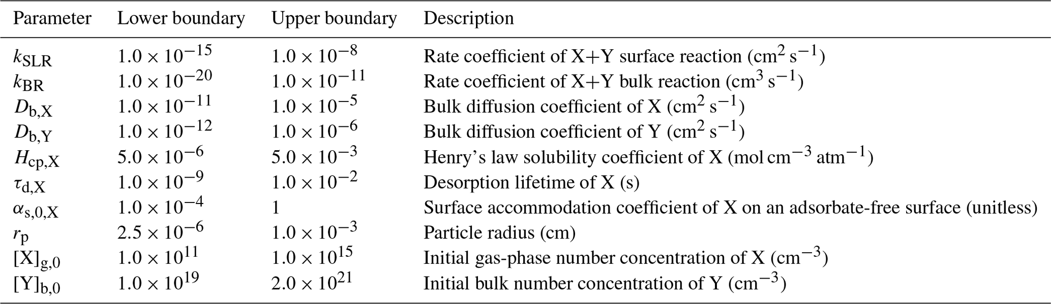
For each input parameter of KM-SUB, individual parameter boundaries are defined, representing a wide array of reactants and scenarios that can be found in either the atmosphere or in laboratory experiments (Table 1). As these ranges cover orders of magnitude, they are assumed to follow log-uniform probability distributions. The parameter space includes liquid to semisolid particles (as expressed by the reactant diffusivities) from 50 nm to 100 µm in size. Reaction rate coefficients range from reactivity close to the diffusion limit, typical for the OH radical (1×10¹¹ cm³ s⁻¹), down to reactions that are 9 orders of magnitude slower, and they may be associated with reactions involving ozone. The volatile reactant X is given a large variability in terms of partitioning properties (as expressed by surface accommodation coefficient α_s,0 and desorption lifetime τ_d) and solubility properties (as expressed by the Henry’s law coefficient), each varying over several orders of magnitude. The initial concentration of non-volatile reactant Y ranges from 10¹⁹ to 2×10²¹ cm⁻³, which, for an organic substance with a molar mass of 250 g mol⁻¹, corresponds roughly to a molar fraction from 0.5 % in relation to pure particles. The concentration of X in the gas phase is held constant over a simulation and is varied between simulations from a few parts per billion (10¹¹ molec. cm⁻³) to about 200 parts per million (5×10¹⁵ molec. cm⁻³). For the explicit treatment of gas diffusion, we assume a temperature of 298 K and a fixed diffusion coefficient of 0.14 cm² s⁻¹.

2.2 Acquisition of training data

The KM is used to generate a training dataset for the surrogate models by randomly sampling parameters in log-uniform space within their associated boundaries. The number of KM samples obtained in this study is about 4.3×10⁶ and required supercomputing. A random set of 1000 samples is removed from the dataset and withheld from model training for the visualization and validation of fully trained surrogate models. We refer to this set of data as test data.

As not only the computational effort of sampling training data but also the time required for surrogate-model creation increases with the size of the training dataset, the surrogate-model performance is tested on different fractions of the total training dataset in order to find an optimal or sufficient computational expense for a given application (Table 2). Note that the PCE method is only applied to the first nine fractions (50–20 000) due to the computational expense of the method at higher training-set sizes.

2.3 Neural network (NN)

The neural network architecture employed in this study is a multi-layer perceptron (MLP), in which nodes are organized in consecutive layers. MLPs are characterized by a chosen number of so-called hidden layers that connect the visible input and output layers. Each node in a layer is connected with each node in the previous and following layers (fully connected layers). We test MLPs consisting of up to five hidden layers with variable numbers of neurons to determine a network architecture that suits the specified task. A detailed mathematical description of MLP functionality and architecture is given in Appendix A1. The processes of hyperparameter tuning, tested ranges, and suggested values for individual hyperparameters are described in Appendix A2. We apply 5-fold cross-validation to avoid over-fitting of the trained models during hyperparameter tuning (Stone, 1974; Wong and Yeh, 2020).

2.4 Polynomial chaos expansion (PCE)

The PCE surrogate-modeling approach will be briefly summarized here. For more technical descriptions, the reader can refer to Sudret (2008) and Le Gratiet et al. (2017). The principle behind PCE is that the model output Z is decomposed into an infinite series as follows (Ghanem and Spanos, 2003):

$$\begin{array}{}\text{(1)}& Z=\sum _{\mathit{\alpha }\in {\mathbb{N}}^M}{y}_{\mathit{\alpha }}{\mathit{\psi }}_{\mathit{\alpha }}\left(X\right),\end{array}$$

where M is the number of model input variables, α is a multi-index that defines the variable components of the polynomials, y_α refers to coefficients, and ψ_α refers to orthonormal polynomials of either one input variable (representing first-order effects) or multiple input variables (representing interacting effects). The type of orthonormal polynomial in Eq. (1) depends on the probability distribution of the input parameters, with uniform probability distributions being represented by Legendre polynomials and Gaussian probability distributions being represented by Hermite polynomials (Xiu and Karniadakis, 2002). In practice, Eq. (1) is truncated by restricting the maximum degree of the polynomials. We calculate PCE coefficients (y_α) using the implementation of least-angle regression (Blatman and Sudret, 2010) from the open-source MATLAB-based software UQLab (Marelli and Sudret, 2014). This software allows degree-adaptive calculation of the PCE, meaning that PCE models can be constructed from degree 1 to a maximum selected degree, which we set to 14. If the cross-validation error of the model does not decrease over two steps in degree, the algorithm stops, and the PCE with the lowest cross-validation error is selected. All PCEs calculated for this study are equal to or below degree 7 (Table A1).

2.5 Global sensitivity analysis

In global sensitivity analysis, Sobol’ indices describe the contribution of uncertainty from each input parameter and interactions between input parameters (Sobol', 2001). The variance D of the model output Z is decomposed into partial variances as follows:

$$\begin{array}{}\text{(2)}& \begin{array}{rl}D& =\text{Var}\left(Z\right)=\sum _{i=\mathrm{1}}^M{D}_i+\sum _{\mathrm{1}\le i<j\le M}{D}_{ij}\\ & +\text{higher order terms},\end{array}\end{array}$$

i.e., the sum of first-order partial variances (D_i), second order partial variances (D_ij), and higher order terms. Sobol’ indices (S) are calculated by normalizing the partial variances by the total variances, e.g., $S_i=\frac{D_i}{D}$ for the first-order contribution of ith input parameter and $S_{ij}=\frac{D_{ij}}{D}$ for the contribution of the interaction between the ith and jth input parameters to the model uncertainty. In order to summarize the overall influence of a specific input parameter, including interactions, a total Sobol’ index ($S_i^T$) can be calculated:

$$\begin{array}{}\text{(3)}& S_i^T=S_i+\sum _{j\ne i}^M{S}_{ij}+\sum _{j\ne i}\sum _{\begin{array}{c}k\ne i\\ k\ne j\end{array}}{S}_{ijk}+\mathrm{\dots }+S_{ij\mathrm{\dots }M}.\end{array}$$

Given the similarities between the PCE and Sobol’ decompositions, the Sobol’ sensitivity indices can be calculated analytically from the PCE coefficients rather than with Monte Carlo sampling (Sudret, 2008). This eliminates a potentially computationally expensive step of the sensitivity analysis process using other surrogate models.

2.6 Acquisition of fit ensembles

With the trained NN model, we illustrate and test the application of surrogate models in inverse-modeling approaches with KM-SUB. Six sets of experimental data of the well-studied oleic acid ozonolysis heterogeneous reaction system (Hearn and Smith, 2004; Ziemann, 2005; Gallimore et al., 2017; Berkemeier et al., 2021) are used to determine kinetic parameter sets that minimize the mean squared (absolute) logarithmic error (MSLE) between model and experiments. More details about the specific optimization problem can be found in Appendix B.

$$\begin{array}{}\text{(4)}& \text{MSLE}={\displaystyle \frac{\mathrm{1}}{N}}\sum _{i=\mathrm{1}}^N{\displaystyle \frac{\mathrm{1}}{n}}\sum _{j=\mathrm{1}}^n\left({\log }_{\mathrm{10}}\right(z_{ij})-{\log }_{\mathrm{10}}(y_{ij}){)}^{\mathrm{2}},\end{array}$$

where N is the number of experimental datasets, n is the number of data points in each set, z_ij is the model output, and y_ij is the value for experiment i and data point j. As this optimization problem does not offer a unique solution (Berkemeier et al., 2021), the aim is not to find a best-fitting parameter set but rather to find a fit ensemble, i.e., an array of parameter sets that all yield a sufficient agreement of the associated KM-SUB outputs with the experimental data. The fit ensemble then not only represents the ranges to which kinetic input parameters could be constrained but is also a means of assessing the uncertainty associated with the KM-SUB model fit when extrapolating the model to environmental conditions outside the calibration range (Berkemeier et al., 2021). For both purposes, the number of model fits in the ensemble must be sufficiently large to fully grasp the remaining model flexibility. The process of determining such a large set of fits can be computationally expensive. A surrogate model can either fully replace the KM or assist in the fitting process by suggesting sampling points.

In this study, we evaluate the benefits of surrogate-model-supported sampling by comparing the distribution of KM-SUB output MSLE for three different sampling approaches within the parameter boundaries presented in Table 1. These approaches are

• random log-uniform sampling,

• Metropolis–Hastings algorithm (MHA)-directed sampling,

• NN-suggested sampling.

We choose an MSLE of 0.016 as representing sufficient agreement between model and experiment. For NN-suggested sampling, we perform a random log-uniform screening of the NN surrogate model in batches of 10 000 samples until we find 5000 NN-suggested fits with MSLE <0.016; we then feed these pre-sampled parameter sets into KM-SUB. We refer to KM-SUB outputs with an MSLE below 0.016 as fits.

As a directed-sampling approach, we apply the Metropolis–Hastings algorithm (MHA), a common Markov chain Monte Carlo method to sample multivariate distributions with high numbers of dimensions (Chib and Greenberg, 1995; Robert and Casella, 1999). We determine the maximum step size of the MHA by basic testing on smaller subsets, and we find that a step size of 0.1 is a good compromise between a high acceptance ratio and sufficient exploration of the entire parameter space. Here, step size is defined as the maximal parameter variation as a fraction of the total logarithmic parameter space. For comparability of the aggregate computational effort, each sampling is performed on an 11th Generation Intel(R) Core(TM) i5-1145G7 CPU with 2.6 GHz.

2.7 Hardware and software tools

Training-data acquisition with KM-SUB was performed in MATLAB on the high-performance computing system Cobra at the Max Planck Computing and Data Facility (MPCDF). Model training of the NN was performed in Python 3.6 using the packages Keras 2.3.0 (Chollet et al., 2015), TensorFlow 1.14.0 (Abadi et al., 2015), scikit-learn 0.22.1 (Pedregosa et al., 2011), NumPy 1.18.1 (Harris et al., 2020), and pandas 0.25.3 (McKinney et al., 2010). Each model training was conducted on one NVIDIA GeForce GTX 1080 Ti on the high-performance computing cluster Mogon of the Johannes Gutenberg University Mainz. For the PCE and sensitivity analysis, we use the MATLAB-based software UQLab 1.3 (Marelli and Sudret, 2014), which provides a framework for surrogate modeling and uncertainty quantification. We performed PCE calculations on ETH Zurich's high-performance computing cluster Euler, using four CPUs per PCE calculation and up to 45 GB of memory for the largest sample size (20 000).

To determine training times of the NN and PCE models, the required time for sample loading and file writing is disregarded, and only the true training time is reported. For the PCE method, the time to reach 90 %, 50 %, and 10 % of the initial amount of Y, N_Y,0, is calculated by three separate models, and training times are added to yield a combined training time for each training sample size. For the NN method, one model can be set to return multiple values as output; thus, a single model is used for each dataset to predict all three output values collectively.

Table 2 Training times of surrogate models with the NN and PCE method.

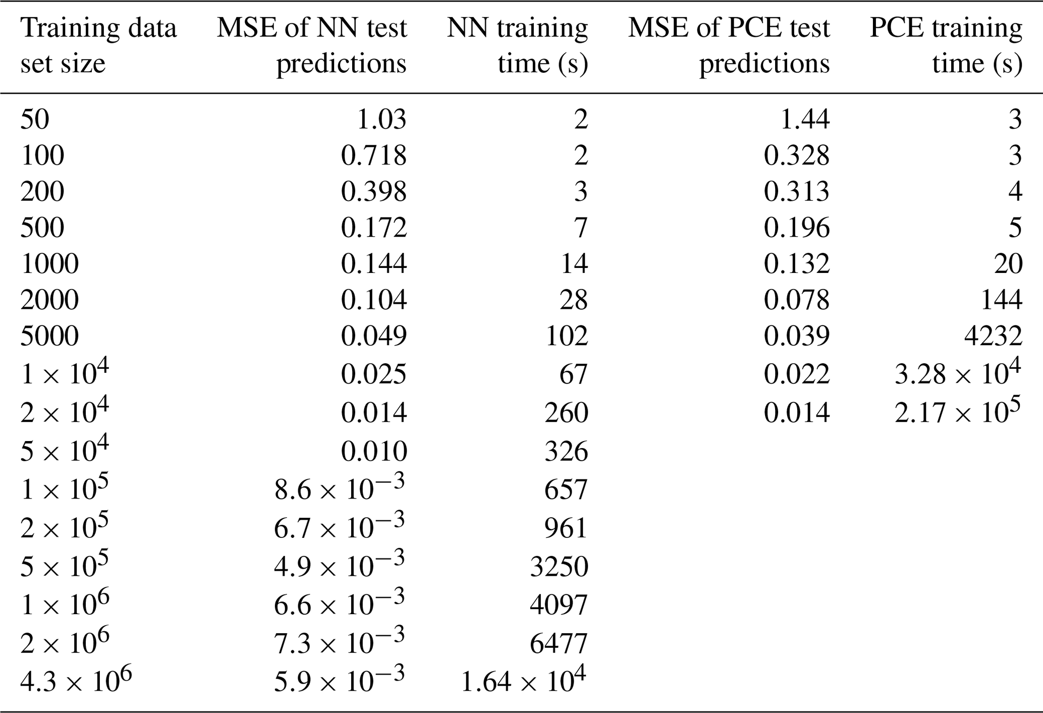
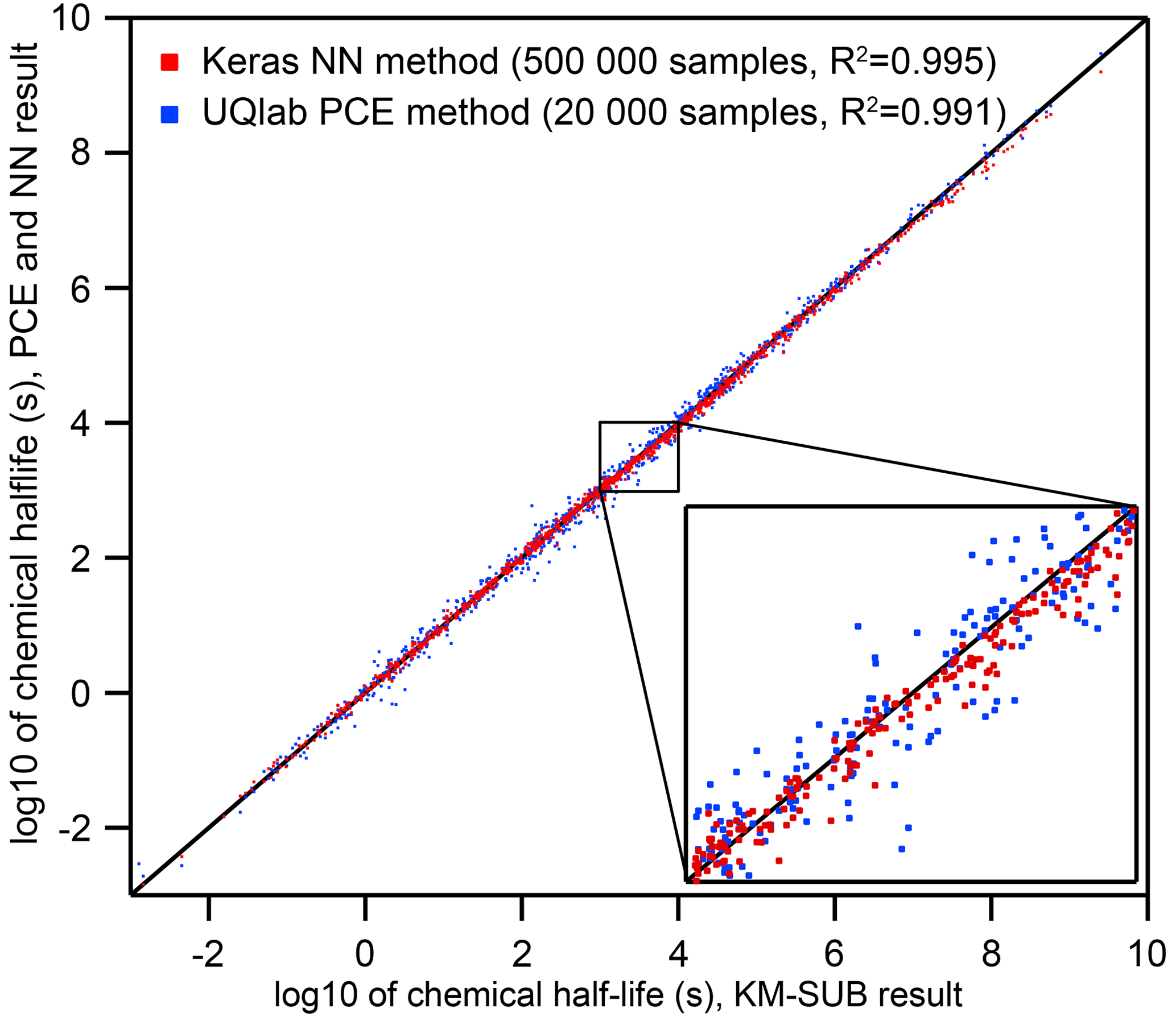
Figure 2 Comparison of the two surrogate models predicting the chemical half-life for heterogeneous chemistry on aerosol particles for a wide range of KM-SUB output (N=1000 – test dataset not part of the training dataset). The surrogate models were trained on 20 000 (PCE) and 500 000 (NN) KM-SUB data samples, respectively. Training times of models with this complexity fall below an upper feasibility range on a personal computer within a few days of time. The inset shows a magnified section and spans from chemical half-lives of 10³ s (≈15 min) to 10⁴ s (≈3 h), a common range for laboratory experiments.

3 Results and discussion

3.1 Surrogate-model training, accuracy, and speed

Neural networks (NNs) and polynomial chaos expansion (PCE) are used to emulate the reaction time of a multiphase chemical system in KM-SUB. Table 2 displays the test set errors and training times of surrogate models with the NN and PCE methods as a function of training-dataset size. The best surrogate models achieve mean square errors (MSEs) for logarithmic reaction times of 0.0049 for the NN method and 0.0137 for the PCE method. This corresponds to correlation coefficients R² of 0.995 and 0.991, respectively. Figure 2 shows that these optimal versions for both surrogate models track the chemical half-life in the test dataset remarkably well. The MSE of test predictions is very similar between both approaches for the same training-dataset size. Error variance of the five cross-validation NN models for the unseen test data is very low at $\mathrm{2.98}\times {\mathrm{10}}^{-\mathrm{6}}$, indicating little to no over-fitting. We found no significant correlations between surrogate-model error and the values of the 10 model input parameters (Fig. S1 in the Supplement).

For dataset sizes above 2000, the PCE model requires much more training time than the NN model. However, note that these training times of individual NN models disregard the necessity of hyperparameter tuning. While hyperparameter tuning is not required in an already established application, the total computation times of NN surrogate-model training and hyperparameter tuning can be 2 orders of magnitude larger, depending on the extent of the hyperparameter tuning that is performed. Hence, the use of an NN method is advisable when a large amount of training data are easily available and when model accuracy is of high importance.

The PCE method, on the other hand, is limited in terms of training-dataset size (≤20 000) as a result of the calculation time and memory requirements in MATLAB. The PCE method is thus a good choice if the training dataset is small or if its acquisition is time limiting and when time-consuming hyperparameter tuning is not desired.

Both surrogate models calculate new output data orders of magnitude faster than the full model, KM-SUB. The computation time of KM-SUB lies on the order of a few seconds per model run, while both the PCE and NN methods can generate large arrays of 10 000 individual surrogate-model solutions in under 1 s.

3.2 Prediction of chemical loss and half-life

Figure 3 visualizes the accuracy of the surrogate models (training-set sizes 20 000 for PCE method and 500 000 for NN method) by generating five concentration–time curves from various input parameter combinations and comparing them to the full KM-SUB model. Input parameter sets were arbitrarily selected from the test set so that the results were spaced out homogeneously across KM-SUB chemical half-lives. We see that, over the wide range, both surrogate models closely represent the KM output, with the NN method slightly outperforming the PCE method as result of the larger training-set size.

Note that both methods are able to produce relatively good surrogate models (MSE ≈0.1) from only 1000 training-data samples (Table 2), which, depending on the user's application, may already be accurate enough. We conclude that KM-SUB is a rather well-behaved model and that it is suitable for these surrogate-modeling techniques.

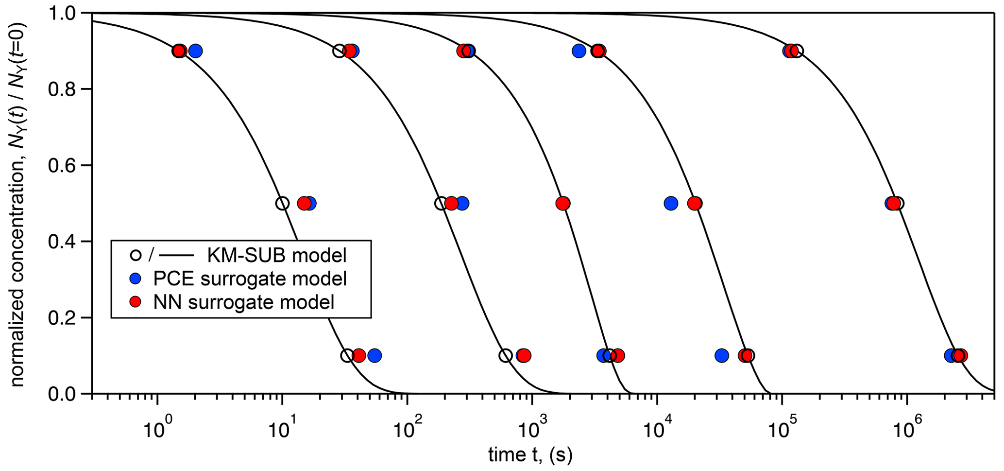
Figure 3 Comparison of time-dependent output of the surrogate models (PCE method – blue markers; NN method – red markers) with KM-SUB model output (solid black lines) for five arbitrarily chosen KM-SUB runs spanning seconds to weeks of reaction time. The surrogate models' predicted time for depletion of 10 %, 50 %, and 90 % of reactant Y in the aerosol phase. KM-SUB output at these three stages is highlighted with open black markers.

3.3 Global sensitivity analysis with surrogate models

An advantage of using a PCE surrogate model is that the Sobol' sensitivity indices can be extracted analytically (Sudret, 2008). We present the global sensitivity analysis for the 50 % lifetime (i.e., the chemical half-life) PCE model in Fig. 4. We can differentiate between first-order effects of a model input parameter, wherein the parameter alone influences the output, and interaction effects, wherein combinations of parameter values influence the output. In Fig. 4, first-order effects dominate the total effect, accounting for 88 % of the model variance. Using the total Sobol' indices (S^T) as a metric, we can assess the overall influence of individual model parameters on the uncertainty of the model output. The input parameters with the largest influence on the chemical half-life of Y are the initial gas-phase concentration of X ([X]_g,0, S^T=0.36) and the radius of the particle (r_p, S^T=0.22). Certain parameters have a very low influence (S^T≤0.05) on the chemical half-life, including the accommodation coefficient (α_s,0,X), the initial concentration of Y ([Y]_b,0), and the bulk diffusion coefficient of Y (D_b,Y). This means that variations in these parameters will, in many cases, not have a large effect on the chemical half-life, indicating that it will be difficult to constrain these parameters with measurements. Sensitivity analysis is thus a useful tool to understand model behavior and to identify parameters which have the largest influence on model output.

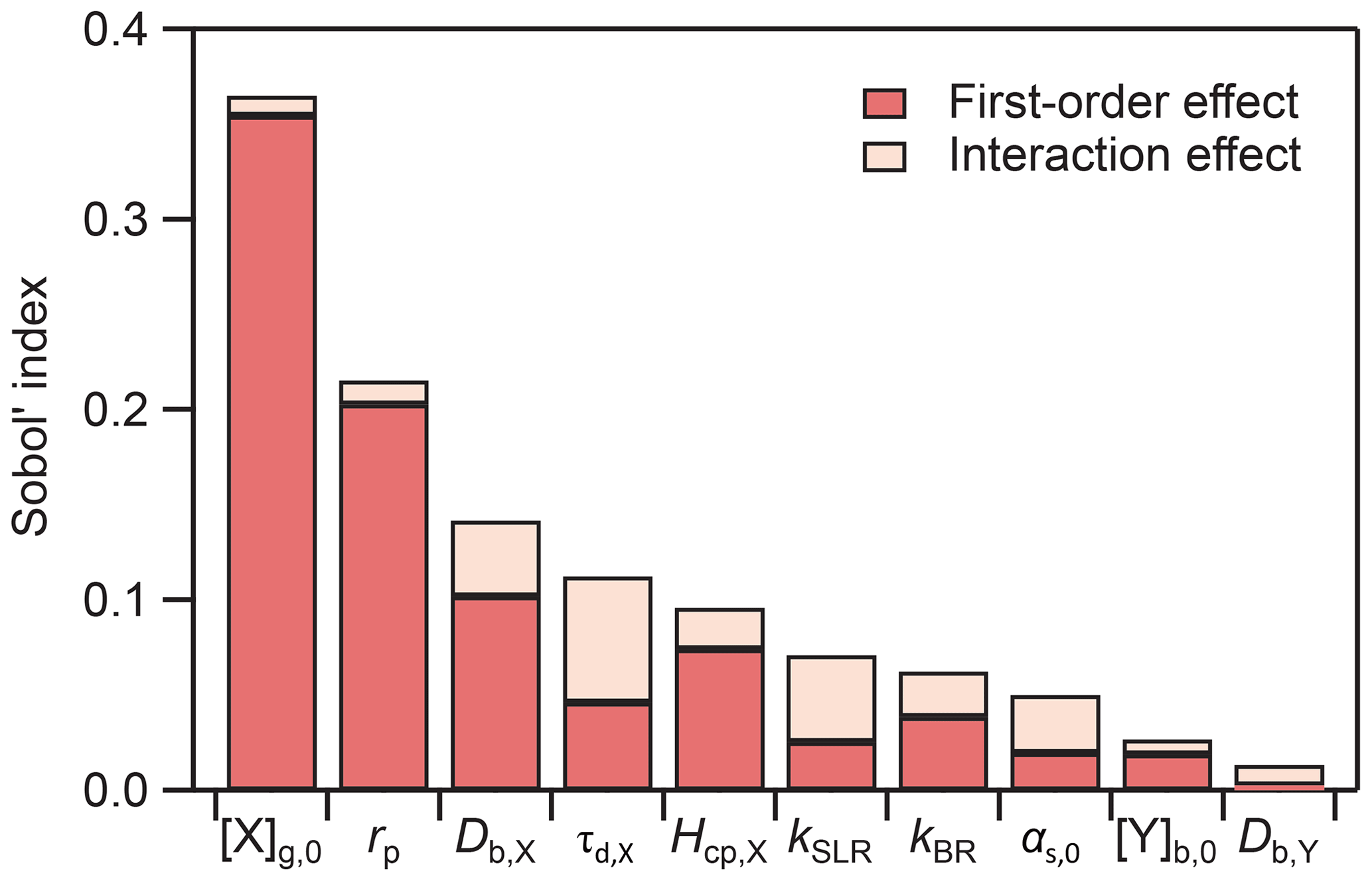
Figure 4 Results of global sensitivity analysis showing Sobol' sensitivity indices for the chemical half-life PCE model.

It has to be noted that a low global sensitivity across the entire input parameter space does exclude the possibility that pockets in the parameter space exist where either of these parameters are very influential. Constraining the input parameter space to smaller subsets can constrain the model to special kinetic regimes or limiting cases that exhibit characteristic profiles of parameter sensitivity (Berkemeier et al., 2013).

In most laboratory experiments, the particle radius and the initial concentration of X are known values. By fixing these parameters in the sensitivity analysis, a substantial fraction of the model variance is eliminated, and other unknown parameters account for a more significant fraction of the overall model variance. To demonstrate how the importance of parameters varies over different experimental conditions, we conducted sensitivity analyses by sampling the PCE surrogate model for specified values of [X]_g,0 and r_p (Fig. 5a). Certain input parameters are consistently important across the range of experimental conditions, e.g., oxidant diffusivity (D_b,X) and solubility (H_cp,X). Other parameters, including k_BR and τ_d,X, have varying influences depending on the experimental conditions. For example, at a high [X]_g,0 and for large r_p, the total Sobol' index of τ_d,X is 0.14. Accordingly, the upper panel of Fig. 5b shows that the chemical half-life of Y only decreases slightly with increasing τ_d,X. In contrast, at low [X]_g,0 and for small r_p, the total Sobol' index increases to 0.31. In the lower panel of Fig. 5b, the chemical half-life of Y shows a stronger dependence on τ_d,X. This can be understood because, for small particles, surface processes are more important, and the surface concentration of X depends on its lifetime for desorption, especially at low gas-phase concentrations. This information could be potentially useful for an experimental researcher, as it shows that experiments at low [X]_g,0 and small r_p could be more helpful for constraining τ_d,X than experiments under other experimental conditions.

These calculations would have been very time consuming when carried out with the full KM. Hence, the combination of surrogate modeling and sensitivity analysis is a helpful yet underutilized tool for designing experiments that are best suited to constraining certain model parameters.

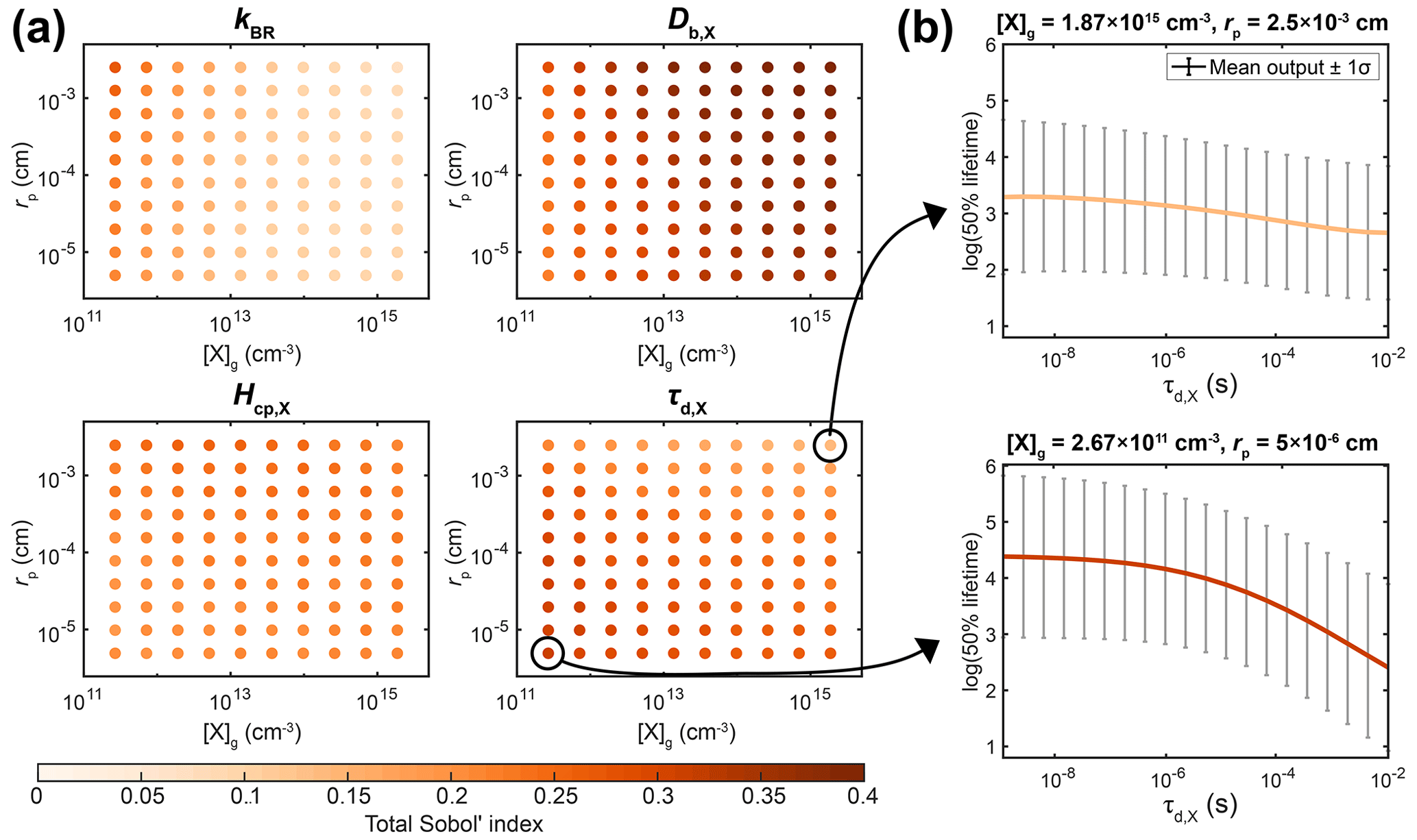
Figure 5 Detailed sensitivity analysis with the PCE method as a function of experimental conditions, i.e., the gas-phase concentration of X ([X]_g,0) and particle radius (r_p). (a) Total Sobol' indices of four KM input parameters: bulk reaction rate coefficient of X and Y (k_BR), bulk diffusion coefficient of X (D_b,X), solubility coefficient of X (H_cp,X), and desorption lifetime of X (τ_d,X). (b) Relationship between the value of τ_d,X and the chemical half-life of Y for two selected experimental conditions.

3.4 NN-supported global optimization

Utilizing the NN surrogate model, we illustrate the accelerated acquisition of parameter sets associated with KM-SUB outputs in good agreement with experimental data, which is the key step in inverse-modeling and optimization approaches. While uncertainty is introduced by surrogate models, their predictions can be obtained orders of magnitude faster than regular KM-SUB calculations. The uncertainty introduced by the NN method can be minimized by additional sampling of a much smaller number of parameter sets with the KM. Re-sampling of NN-suggested solutions with the KM can avoid collection of false-positive fits (i.e., meeting the conditions for a fit in the NN model but not in KM-SUB), and sampling in close vicinity of NN-suggested solutions might avoid false-negative fits (i.e., not meeting the conditions for a fit in the NN model but in KM-SUB).

We perform random parameter sampling in log-uniform space using the boundaries presented in Table 1, and we find about 5000 NN-suggested fits in 1.84×10⁷ parameter sets (0.027 % acceptance), requiring a total of 13 847 s (<4 h). A comparable calculation with KM-SUB would take years on a desktop computer or days on a supercomputer. In contrast, re-sampling of the NN-suggested fits with KM-SUB to avoid false-positive fits is time-consuming but feasible. The time required for sampling 5000 kinetic parameter sets (i.e., 5000×6 runs in KM-SUB) on a desktop computer ranges from 51 646 s (≈14 h) for NN-suggested sampling to 103 530 s (≈29 h) for random log-uniform sampling. The differences may be a result of the fraction of parameter sets where differential equation calculations of the KM require a very long time to terminate. They are often associated with very long reaction times and thus with large MSLEs.

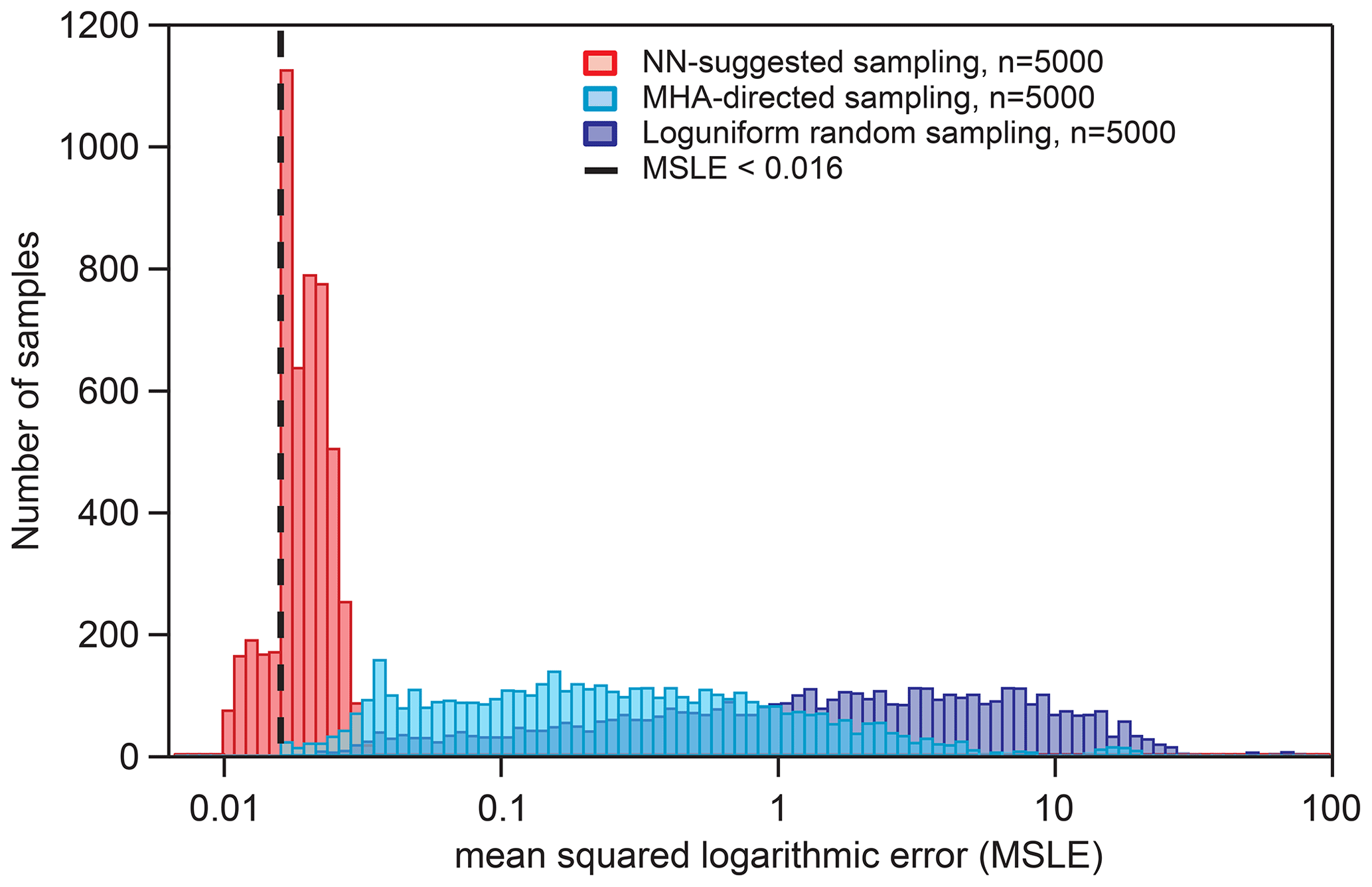
Figure 6 Distribution of KM-SUB output MSLEs for three different sampling methods in comparison with six sets of experimental data, as described in Sect. 2.6. The dashed vertical line represents the threshold used for the acquisition of NN-suggested fits (MSLE <0.016). The maximum step size for the MHA-directed sampling is 0.1.

Figure 6 shows the distributions of KM-SUB output MSLE for three different sampling methods: log-uniform random sampling, MHA-directed sampling, and NN-suggested sampling (Sect. 2.6). The NN-suggested sampling method greatly outperforms both random and MHA-directed sampling. The number (fraction) of KM-SUB outputs with an MSLE <0.016 is 1602 (32.04 %) for NN-suggested sampling, 21 (0.42 %) for directed KM-SUB sampling, and 3 (0.06 %) for random sampling.

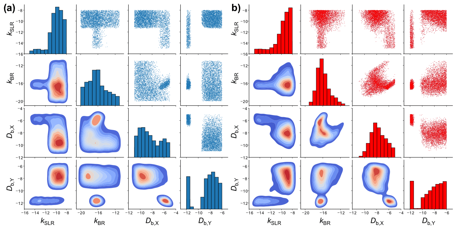
Figure 7 Scatter plot matrices of the fitting parameter space of 5000 fits to six experimental datasets of the ozonolysis of oleic acid aerosols (Appendix B) obtained with (a) KM-SUB and (b) the NN surrogate model. Shown are four out of seven optimized kinetic parameters. The diagonal elements are histograms showing the distributions of the individual fit parameter densities. The off-diagonal elements are scatter plots (top right) or densities (bottom left) of solutions for all possible combinations of two kinetic parameters. The KM-SUB fit ensemble originates from the application of the MHA with a step size of 0.1 and the NN fit ensemble from log-uniform random sampling.

Figure 7 compares the fitting parameter space of 5000 fits obtained with KM-SUB (panel a) and the NN surrogate model (panel b), exemplary for four kinetic parameters in a so-called scatter plot matrix. The off-diagonal elements in each matrix show bivariate scatter plots (top right) or density plots (bottom left) depicting the relationship of two kinetic parameters within the fit ensemble. The diagonal elements are histograms showing frequency distributions of the individual parameters. The two scatter plot matrices show a clear resemblance in terms of the fit parameter spaces between the surrogate model and the original KM. Much like the scatter plots of the original-model fits, the scatter plots of the surrogate-model fits can be used to identify areas that will not produce a fit to experimental data. For example, there are no fits with a slow surface reaction rate coefficient (k_SLR) and a high oxidant solubility (H_cp,X). However, some features in the scatter plots of the surrogate model deviate from those in the scatter plots of the original KM. We can visually identify areas in the scatter plots that indicate false-positive fits, i.e., areas that are only occupied in the plots for the surrogate model. An absence of density in other areas, compared to the plots for the original model, suggests the existence of false-negative fits.

Whether it is worthwhile to train a surrogate model for a given optimization task depends strongly on the complexity of the KM and the difficulty of the optimization problem. For every application, there is a break-even point where the computational expense of training a surrogate model is compensated for by the acceleration of the optimization task(s). In this study, the computational effort required to obtain the training data for the best-performing surrogate model (500 000 KM-SUB sample runs) would only find ∼350 fits if we had directed this initial sampling effort into fit acquisition using only KM-SUB. This is due to the very low fraction of fits (0.42 %) without the aid of surrogate models and because KM-SUB has to be evaluated six times, once for each laboratory dataset. Thus, if the uniqueness of an optimization result must be determined, large amounts of laboratory data are available, or simply, if global optimization of the same model is required on a regular basis, training of a surrogate model for this task quickly becomes worthwhile.

4 Conclusions

In this study, we illustrate the application of artificial neural networks (NNs) and polynomial chaos expansion (PCE) to generate fast surrogate models for computationally expensive kinetic models (KMs). As a template KM, we use the kinetic multi-layer model of aerosol surface and bulk chemistry (KM-SUB; Shiraiwa et al., 2010), but the presented methods can equally be applied to other process models. To reduce data storage requirements in sampling and to simplify emulation, the complex model output of KM-SUB, i.e., the concentration profiles of all reactants over space and time, is reduced to the reaction time of the system to reach a certain reaction progress, as this is a typical observable in laboratory experiments. We note that other derivatives of KM-SUB model output, such as the uptake coefficient of the reactant gas to the aerosol surface, could be chosen depending on the target application of the surrogate model. Emulation of the entire KM-SUB output may be feasible and could be facilitated by data compression methods such as auto-encoders, singular-value decomposition, or principal component analysis.

Our findings suggest that, after an initial investment of computational effort for training-data sampling and model training, both methods yield models with very good correlations to KM-SUB outputs (R²>0.99). Furthermore, we provide examples for the application of such surrogate models for inverse modeling and kinetic parameter optimization: global sensitivity analysis with the PCE method and acceleration of global optimization with the NN method. The results indicate that surrogate models can aid in costly optimization tasks or help to select environmental system parameters for experiments that significantly constrain KM solution space and thus global fit uncertainty.

It is important to note that errors of surrogate models are not simply based on a random deviation of surrogate-model predictions from the values of the original KM but on a divergence of the predicted parameter hyper-surface in specific areas, for instance where training data are sparse. False-positive fits, i.e., parameter sets with associated surrogate-model predictions in better agreement with experimental data as the delineated KM output, can simply be eliminated by re-sampling the parameter sets in question with the KM (Fig. 6). On the other hand, false-negative fits and their implications for inverse-modeling approaches are much more difficult to address. While optimization hyper-surfaces can be scanned relatively quickly with a surrogate model, this is not the case for the much slower KM. Scatter plot matrices of the fitting parameter space are a valid means of identifying areas that are occupied by false-negative fits, but a proper comparison (Fig. 7) requires computationally costly sampling with the KM.

Another potential application of surrogate models for KM is their utilization as modules in large-scale chemical transport models. As such models often require many calls of the respective module, direct use of models such as KM-SUB, where calculation time is on the order of seconds, is not feasible. Trained, predictive surrogate models, however, can easily be integrated into existing modeling programs. This potentially allows the coupling of small-scale kinetic process models with large-scale chemical transport models for the simulation of weather, pollution, and climate. Kelp et al. (2022) recently demonstrated acceleration of a global model with an online-learned NN as a chemistry module. The machine learning models presented in this study could be embedded in existing FORTRAN code in a similar fashion.

Appendix A: Neural networks

A1 Neural network architecture

A multi-layer perceptron (MLP) represents a complex, non-linear function that maps an input to an output vector. Each individual node in an MLP represents a non-linear function, mapping from the sum of its inputs to an output, which is passed to the following interconnected nodes. Connections between nodes are associated with weights that are optimized during training in order to reduce model output error in comparison with the dataset values. For this purpose, an optimization algorithm is used to minimize a previously defined loss function based on the final model output. In their entirety, these weights determine the output of the MLP based on a specific input, and their adaptation, based on the training data, represents the learning process. The following equations show the principal mathematical functionality of neurons in an MLP, as elaborated upon in Kröse and van der Smagt (1996):

$$\begin{array}{}\text{(A1)}& s_k\left(t\right)=\sum _j{w}_{jk}\left(t\right)y_j\left(t\right)+{\mathit{\Theta }}_k\left(t\right),\end{array}$$

where s_k(t) is the effective input of a neuron k at time t, w_jk is the weight between neuron j and k, and y_j(t) is the activation of the previous neuron j. This equation represents the input of a single computational node in the NN, which is based on the activation of connected previous nodes and the associated (trained or initialized) weights. Θ_k(t) represents an offset term. Of this so-called propagation rule, different adaptations have been proposed (Feldman and Ballard, 1982).

$$\begin{array}{}\text{(A2)}& y_k(t+\mathrm{1})=F_k\left(y_k\right(t),s_k(t\left)\right))\end{array}$$

This equation introduces the activation function of neuron k (F_k) that maps the neuron input s_k(t) and the current activation y_k(t) of the neuron to a new activation value. A common type of the activation function is a sigmoid-like function, as shown in the following equation:

$$\begin{array}{}\text{(A3)}& y_k=F\left(s_k\right)={\displaystyle \frac{\mathrm{1}}{\mathrm{1}+e^{-s_k}}}.\end{array}$$

The definition of the input and activation functions of neurons determines the output of any NN given a specific input and a set of weights. NN model training or learning describes the process of iterative modification of weights in order to shift the output in a desired way. In most cases, this desired shift is a reduction of error towards the associated predictable values in the underlying population associated with the training data. If the model is well fitted to the training data but predicts further data of the same population with much larger error, it is referred to as over-fitted. Over-fitting describes overall ill generalization of an NN model. A common learning rule for nodes, the so-called perceptron learning rule, is shown in the following equation:

$$\begin{array}{}\text{(A4)}& w_i(t+\mathrm{1})=w_i\left(t\right)+\mathit{\Delta }{w}_i\left(t\right).\end{array}$$

Table A1 Employed polynomial degree of the three PCE models (90 %, 50 %, and 10 % lifetime) as function of training-dataset size.

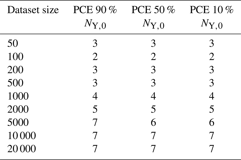
Table A2 Descriptions and tested ranges for neural network hyperparameters used in the Python package Keras, as well as the recommendation based on our best-performing model.

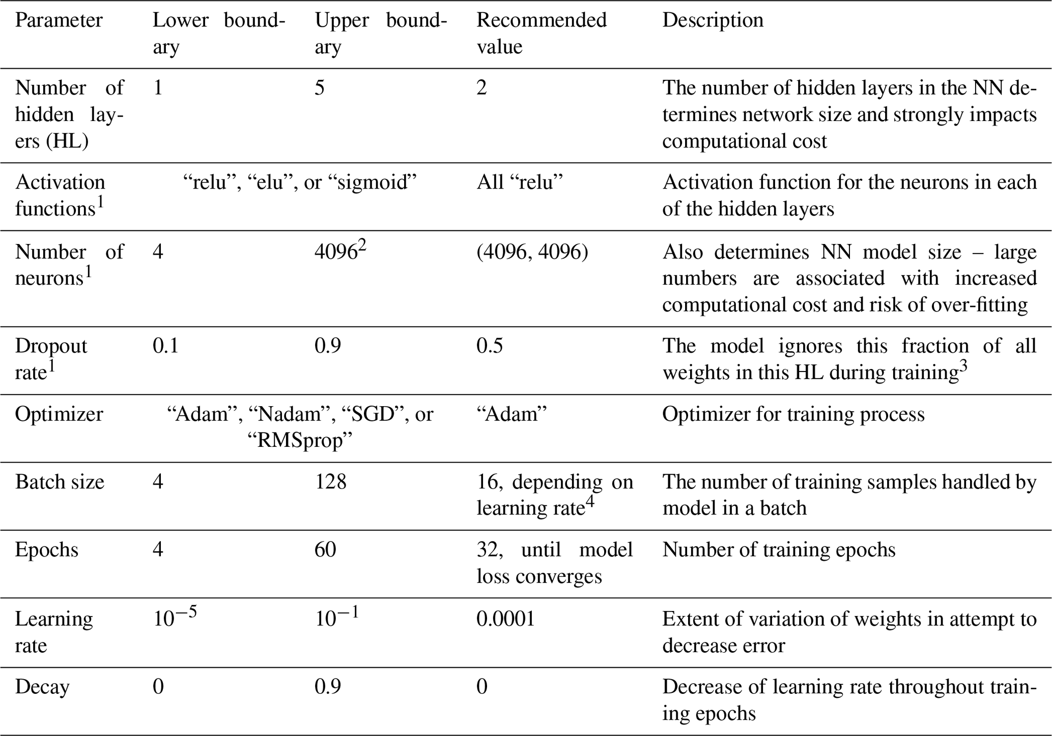
¹ Must be set for each individual HL. ² Larger numbers of neurons per layer lead to over-fitting and, with the hardware setup in this study, memory limitations on the computational cluster. ³ A random fraction of weights obtained in previous training, determined in size by this parameter, is not considered during the current training. This handicap or restriction ensures that the model is not capable of just saving or learning all the inputs and associated outputs in the training dataset throughout multiple training epochs (as this would be over-fitting). ⁴ A larger batch size decreases training time and requires higher learning rates.

In order to adjust the weights, the output of the NN is compared with the associated training-data values. If the prediction is inaccurate, the modification Δw_i is applied. For this iterative adjustment to be target-oriented, an optimizer is necessary to reduce the prediction error of the NN during training. Different optimizers are commonly used in machine learning applications, such as simple gradient methods like stochastic gradient descent (SGD), where an estimate of the gradient (the direction of the steepest descent) along with a selected step size determines the variation of input parameters in the current step. As information in a feed-forward NN, like an MLP, is only passed in one direction, a method called back propagation is used to determine the direction and amount of weight adjustment in previous NN layers based on the error of the final prediction. More in-depth explanations, definitions, and examples for back propagation and optimization throughout the learning process can be found in Rumelhart et al. (1995) and Hecht-Nielsen (1992); for further information regarding MLPs and NNs in general, see Almeida (2001) or Popescu et al. (2009).

A2 Hyperparameter tuning

Comprehensive hyperparameter tuning is conducted every time a surrogate model is trained on different training data. In this study, we focus on the investigation of dataset sizes and training times. For this reason and because our application of NN is not very common and only a small amount of information regarding successful model architectures and hyperparameters is available, only basic, plain network architectures are tested (i.e., MLPs with up to five fully connected hidden layers and up to 4096 neurons in each of the layers). We perform hyperparameter tuning in three steps, aiming for an optimization of number of layers, layer activation functions, learning rate, and batch size in the first step; number of neurons in each layer in the second step; and dropout rate in the third step. For each step, we apply an adapted grid search where multiple well-performing hyperparameter sets from the previous step are extended by variation of the additionally optimized hyperparameter of the current step.

We performed relatively comprehensive hyperparameter tuning with 60 to 120 hyperparameter sets for each data subset, with each tested set resulting in five models for the individual cross-validation folds. Sets of hyperparameters that lead to well-performing models can, to some extent, be adopted for approaches with similar preconditions regarding the number of inputs and outputs or training-dataset size. For a similar approach, we recommend a basic hyperparameter tuning with at least 10 hyperparameter sets and 5-fold cross-validation. The best models are selected by the average test set error of the five models for each of the cross-validation folds using the mean squared error. The ranges of hyperparameters tested in this study are listed in Table A2 along with the hyperparameter values of the best-performing models for large datasets.

Besides NNs from the Keras package, other deep-learning algorithms tested for this study are the random forest regressor, the decision tree regressor, the SGD regressor, the ridge regressor, least absolute shrinkage and selection operator (LASSO), logistic regression, and the MLP regressor, provided by the Python library scikit-learn (Pedregosa et al., 2011). As most of the tested algorithms did not perform very well in basic tests, we focus on Keras as a common and versatile tool for neural network application.

Appendix B: Oleic acid ozonolysis datasets

In Sect. 3.4, KM-SUB and the NN surrogate model are applied to six experimental datasets of the ozonolysis of oleic acid aerosols – these are available in the literature (Hearn and Smith, 2004; Ziemann, 2005; Gallimore et al., 2017; Berkemeier et al., 2021). These datasets comprise flow tube, environmental chamber, and single-particle levitation techniques and are a subset of data investigated earlier by Berkemeier et al. (2021), omitting the studies that investigated particles with a sodium chloride core or in which the particle size was not measured. The experimental datasets are converted to normalized concentrations (N_Y,t and N_Y,0) and are further simplified by fitting a mono-exponential decay ($A+B\cdot \exp (-{\mathit{\tau }}_{\text{e}}\cdot t)$) and evaluating the reaction time at which 10 %, 50 %, and 90 % of oleic acids are consumed. Table B1 shows the environmental parameters (particle radius r_p, ozone concentration [X]_g,0, and initial oleic acid concentration [Y]_b,0), the derived reaction times, and the mono-exponential fit parameters. The remaining seven KM-SUB input parameters listed in Table 1 are optimized. Figure B2 shows all datasets alongside a fit ensemble of 50 KM-SUB fits with a fit correlation MSLE of less than 0.016.

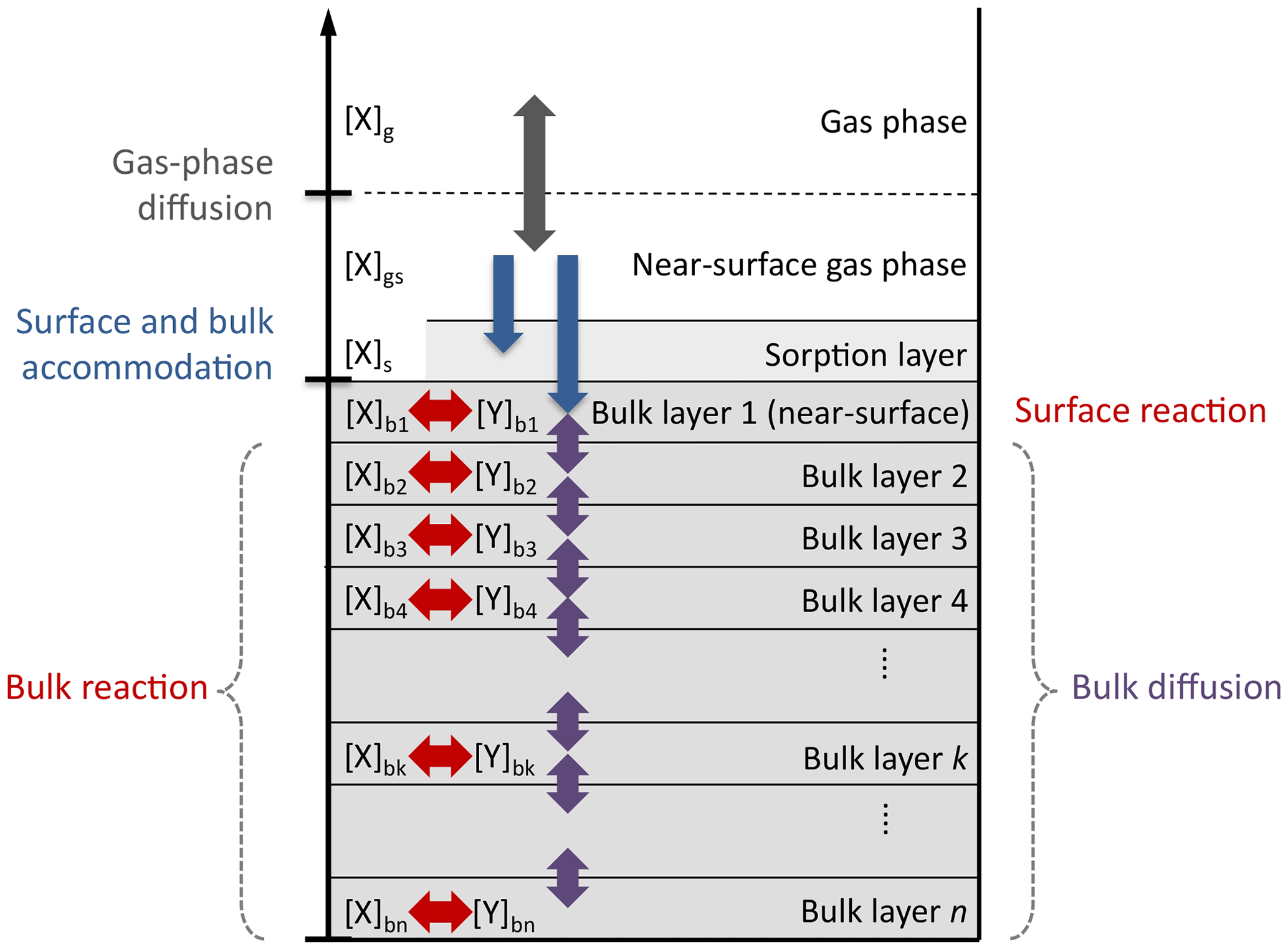
Figure B1 Compartments and processes of the kinetic multi-layer model of aerosol surface and bulk chemistry (KM-SUB).

Berkemeier et al. (2021)Ziemann (2005)Hearn and Smith (2004)Gallimore et al. (2017)Gallimore et al. (2017)Gallimore et al. (2017)

Table B1 Model parameters for the global optimization of six oleic acid ozonolysis datasets.

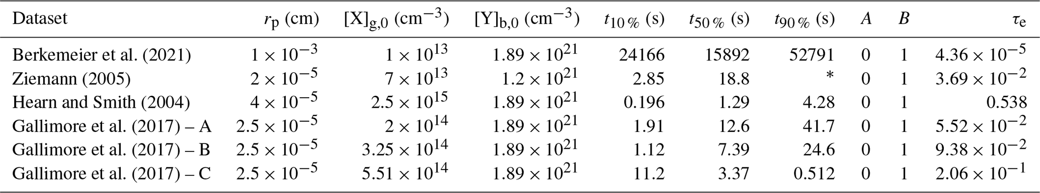
^* Too far outside data range.

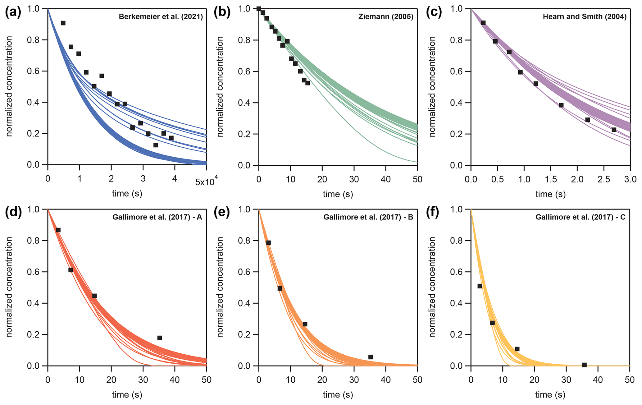
Figure B2 Fit ensembles of KM-SUB (N=50, colored lines) with MSLE <0.016 to six literature datasets (black square markers) of oleic acid aerosol ozonolysis displayed as normalized oleic acid concentrations ($N_{\text{Y},t}/N_{\text{Y},\mathrm{0}}$).

Appendix C: Abbreviations

KM	Kinetic multi-layer model
KM-SUB	Kinetic multi-layer model of aerosol
	surface and bulk chemistry
MHA	Metropolis–Hastings algorithm
MLP	Multi-layer perceptron
MSE	Mean square error
MSLE	Mean squared (absolute) logarithmic error
NN	Neural network
PCE	Polynomial chaos expansion