the Creative Commons Attribution 4.0 License.
the Creative Commons Attribution 4.0 License.
 | 31 Mar 2023
Accelerated estimation of sea-spray-mediated heat flux using Gaussian quadrature: case studies with a coupled CFSv2.0-WW3 system
Ruizi Shi
Fanghua Xu
Sea-spray-mediated heat flux plays an important role in air–sea heat transfer. Heat flux integrated over the droplet size spectrum can simulate well the total heat flux induced by sea spray droplets. Previously, a fast algorithm of spray flux assuming single-radius droplets (A15) was widely used, as the full-size spectrum integral is computationally expensive. Based on the Gaussian quadrature (GQ) method, a new fast algorithm (SPRAY-GQ) of sea-spray-mediated heat flux is derived. The performance of SPRAY-GQ is evaluated by comparing heat fluxes with those estimated from the widely used A15. The new algorithm shows a better agreement with the original spectrum integral. To further evaluate the numerical errors of A15 and SPRAY-GQ, the two algorithms are implemented into the coupled Climate Forecast System model version 2.0 (CFSv2.0) and WAVEWATCH III (WW3) system, and a series of 56 d simulations in summer and winter are conducted and compared. The comparisons with satellite measurements and reanalysis data show that the SPRAY-GQ algorithm could lead to more reasonable simulation than the A15 algorithm by modifying air–sea heat flux. For experiments based on SPRAY-GQ, the sea surface temperature at middle to high latitudes of both hemispheres, particularly in summer, is significantly improved compared with the experiments based on A15. The simulation of 10 m wind speed and significant wave height at middle to low latitudes of the Northern Hemisphere after the first 2 weeks is improved as well. These improvements are due to the reduced numerical errors. The computational time of SPRAY-GQ is about the same as that of A15. Therefore, the newly developed SPRAY-GQ algorithm has potential to be used for the calculation of spray-mediated heat flux in coupled models.
- Article
(13967 KB) - Full-text XML
-
Supplement
(28184 KB) - BibTeX
- EndNote


Sea spray droplets, ejected from oceans, include film drops, jet drops and spume drops (Veron, 2015). The first two types of droplets are generated from bubble bursting caused by ocean surface wave breaking, with radius ranging from 0.5 to 50 µm (Resch and Afeti, 1991; Thorpe, 1992; Melville, 1996; Spiel, 1997; Andreas, 1998; Lhuissier and Villermaux, 2012). Spume drops are generated by strong winds (> 7–11 m s−1) which directly tear the wave crests, with larger radius ranging from tens to hundreds of micrometers (Koga, 1981; Andreas et al., 1995; Andreas, 1998). Sea spray droplets play an important role in weather and climate processes (Fox-Kemper et al., 2022). On one hand, sea spray droplets contribute to local marine aerosols and subsequently modify the local radiation balance (Fairall et al., 1983; Burk, 1984; Fairall and Larsen, 1984). On the other hand, sea spray droplets affect the fluxes of heat, momentum, salt, and freshwater between the atmosphere and ocean (Andreas, 1992; Andreas et al., 2008; Andreas, 2010; Andreas et al., 2015; Ling and Kao, 1976; Fairall et al., 1994; Andreas and Decosmo, 2002).
The sea-spray-mediated heat transfer mainly occurs within the droplet evaporation layer (DEL) near the sea surface (Andreas and Decosmo, 1999, 2002; Fairall et al., 1994). Sea spray droplets with the same temperature as the ocean surface can lead to sensible heat flux in DEL, while water evaporated from these droplets can further release latent heat to the atmosphere (Andreas, 1992; Borisenkov, 1974; Bortkovskii, 1973; Wu, 1974; Monahan and Van Patten, 1988; Ling and Kao, 1976). Part of the sea-spray-mediated sensible heat is absorbed by droplet evaporation, which further increases the air–sea temperature difference and thus increases the sea-spray-mediated sensible heat flux (Fairall et al., 1994; Andreas and Decosmo, 2002). Since strong winds produce more sea spray droplets with a larger radius, sea-spray-mediated heat fluxes increase with wind speed (Fairall et al., 1994) and contribute to more than 10 % of the total surface heat flux after reaching the threshold speed (> 11 m s−1 for sensible heat flux and > 13 m s−1 for latent heat flux) (Andreas et al., 2008). In addition, when a droplet is released into the air, it is accelerated due to surface winds (Edson and Andreas, 1997; Fairall et al., 1994; Van Eijk et al., 2011; Wu et al., 2017). If the droplet could fall back into the ocean, additional momentum would be injected into the ocean from the atmosphere (Andreas, 1992, 2004).
The usual bulk parameterizations in numerical models for surface fluxes only include the interfacial (turbulent) fluxes (e.g., Fairall et al., 1996) while neglecting the significant contributions of sea spray droplets in DEL (Andreas et al., 2008; Fairall et al., 1994; Smith, 1997; Emanuel, 1995). Andreas and Emanuel (2001) implemented sea-spray-mediated heat flux and momentum flux parameterizations into a simple tropical cyclone model and found that the sea-spray-mediated heat flux can significantly enhance tropical cyclone intensity. The similar enhancement of tropical cyclone intensity was also noticed in recent regional coupling systems by including sea-spray-mediated heat flux (Xu et al., 2021a; Liu et al., 2012; Garg et al., 2018; Zhao et al., 2017). In the First Institute of Oceanography Earth System Model, Bao et al. (2020) first incorporated the sea-spray-mediated heat flux in global climate simulation. Following Bao et al. (2020), Song et al. (2022) found that the sea-spray-mediated heat flux can lead to cooling at the air–sea interface and westerlies strengthening in the Southern Ocean, and it thus improves estimates of sea surface temperature (SST).
Since the parameterization of sea-spray-mediated heat flux derived from observations requires full-size spectral integral and thus is computationally expensive for large-scale models (Table 1, details in Sect. 4.2; Andreas, 1989, 1990, 1992; Andreas et al., 2015), a simplified algorithm based on a single radius of sea spray droplets (Andreas et al., 2015, 2008) is widely used in atmosphere–ocean coupling systems (Xu et al., 2021a; Liu et al., 2012; Garg et al., 2018; Zhao et al., 2017; Song et al., 2022; Bao et al., 2020) and is apt to produce numerical errors. To reduce these numerical errors induced by the single radius of sea spray droplets, we develop a new fast algorithm of sea-spray-mediated heat flux based on the Gaussian quadrature (GQ) method, a fast and accurate way to calculate spectral integral. The GQ method has been successfully used for the estimation of domain-averaged radiative flux profiles (Li and Barker, 2018). The performance of the GQ-based fast algorithm of the sea-spray-mediated heat flux is evaluated and compared with the simplified algorithm for single radius of Andreas et al. (2015), referred to as A15 hereafter. The results are first compared with the original parameterization using full-size spectral integral (A92, hereafter). Then, the parameterizations with different algorithms are implemented in a global coupled atmosphere–ocean–wave system (Shi et al., 2022), and the results are compared with global satellite measurements and reanalysis data.
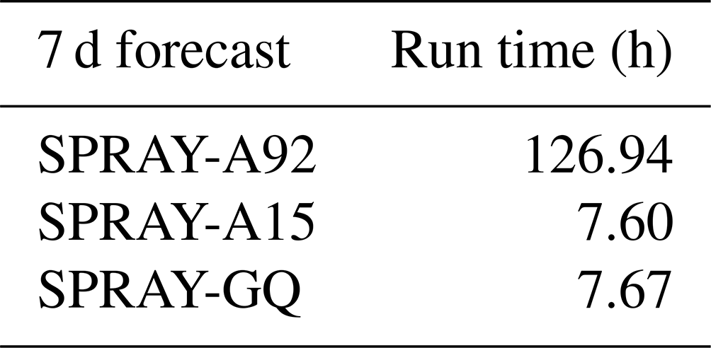
Table 1The run time of the coupled Climate Forecast System model version 2.0 (CFSv2.0) and WAVEWATCH III (WW3) system's global experiments for 7 d forecast with different parameterizations.
The rest of the paper is structured as follows: observation and reanalysis data for comparisons are introduced in Sect. 2, the derivation of the GQ-based fast algorithm and the global coupling system are described in Sect. 3, the performance of the new fast algorithm is evaluated in Sect. 4, and finally, a summary and discussion are given in Sect. 5.
The fifth-generation European Centre for Medium-range Weather Forecasts (ECMWF) Reanalysis (ERA5; Hersbach et al., 2020) 10 m wind speed (WSP10), 2 m air temperature (T02), 2 m dew point temperature, surface pressure, and significant wave height (SWH) with a spatial resolution of 0.5∘ are used. Additionally, WSP10, T02 and 2 m specific humidity (SPH) data from the Objectively Analyzed air–sea Fluxes (OAFlux) products (Yu et al., 2008) are also applied for comparison with 1∘ × 1∘ resolution. The daily average satellite Optimum Interpolation SST (OISST) data are obtained from the National Oceanic and Atmospheric Administration (NOAA) with a spatial resolution of 0.25∘ (Reynolds et al., 2007). The global monthly mean salinity observations from the European Space Agency (ESA; https://climate.esa.int/sites/default/files/SSS_cci-D1.1-URD-v1r4_signed-accepted.pdf, last access: 18 March 2023) are applied. Besides these, we also use the monthly global ocean Remote Sensing Systems (RSS) satellite data products for WSP10 (https://data.remss.com/wind/monthly_1deg/, last access: 18 March 2023) and the reprocessed L4 satellite measurements for SWH (https://doi.org/10.48670/moi-00177, Collecte Localisation Satellites, 2021), to validate the simulation results and ERA5 data.
3.1 Development of a fast algorithm based on GQ
The effects of sea spray droplets on sensible and latent heat fluxes (HS,SP, HL,SP) contribute to the total turbulent sensible and latent heat fluxes (HS,T, HL,T) at the air–sea interface. That is,
where HS and HL are the sensible and latent heat fluxes at the air–sea interface due to the air–sea differences of temperature and humidity. Based on observations of total turbulent heat fluxes and the Coupled Ocean–Atmosphere Response Experiment (COARE) algorithm (Andreas et al., 2015; Fairall et al., 1996), A92 integrates the sea-spray-mediated sensible and latent heat flux spectrums over initial droplet radius (QS(r0) and QL(r0)) to estimate HS,SP and HL,SP (details in Appendix A; Andreas, 1989, 1990, 1992; Andreas and Decosmo, 2002). The distributions of QS(r0) and QL(r0) spectrums as functions of initial droplet radius r0 under various atmosphere and ocean states are shown in Fig. 1, indicating that QS and QL spectrums are more sensitive to the change of WSP10 and less sensitive to other variables, including T02, 2 m relative humidity, SST, surface air pressure and sea surface salinity.
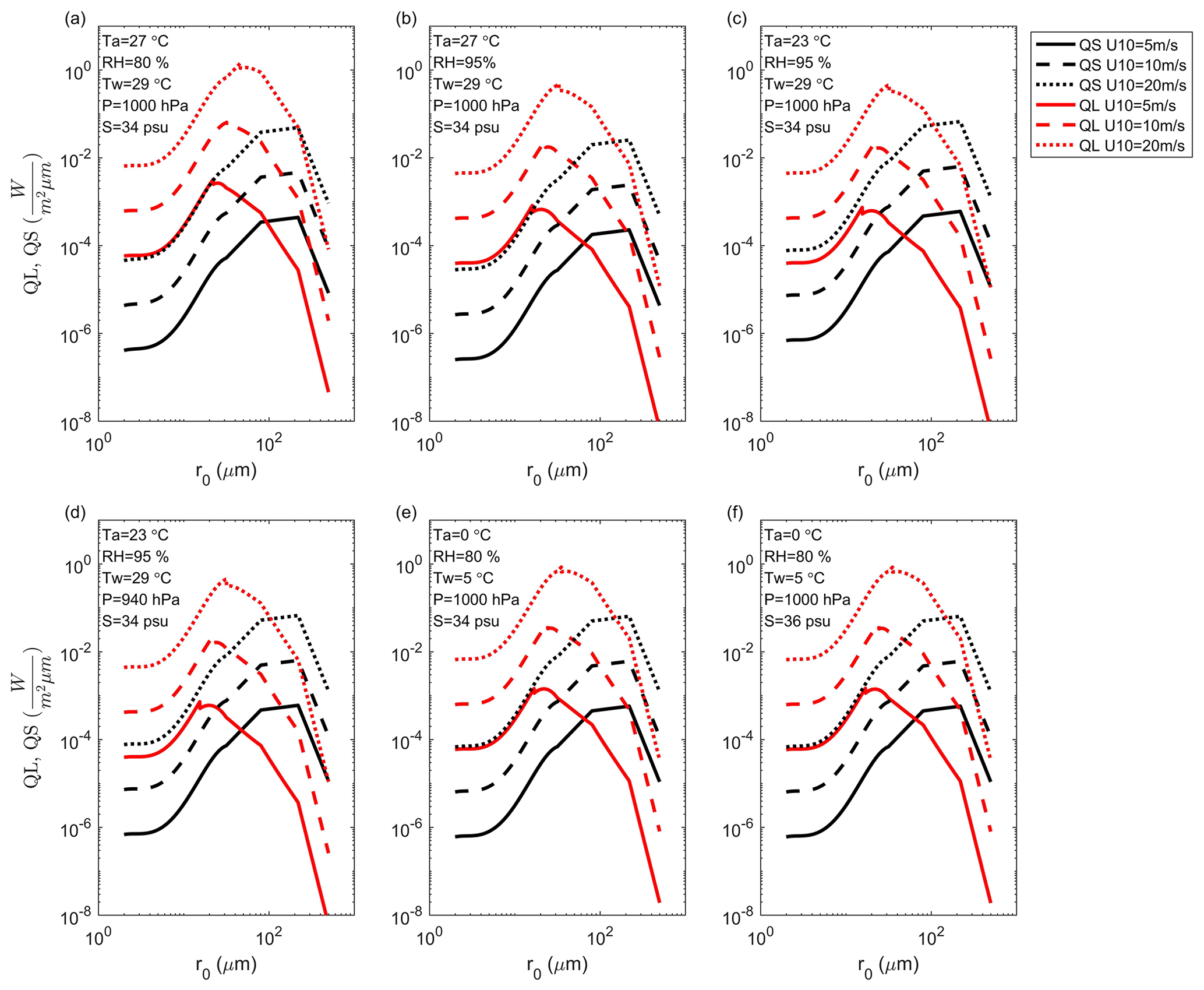
Figure 1The radius-specific sea-spray-mediated sensible (QS: black) and latent (QL: red) heat fluxes as functions of initial radius r0: U10, Ta, RH, Tw, P and S are 10 m wind speed, 2 m air temperature, 2 m relative humidity, sea surface temperature, surface air pressure and surface salinity, respectively.
Since the calculation of HS,SP and HL,SP in A92 is computationally expensive due to full-size spectral integral (Eqs. A5–A6 of Appendix A), it is difficult to apply A92 directly in coupled modeling systems. A15 (Andreas et al., 2015) developed a fast algorithm by using a single representative droplet radius (details in Appendix B), which was widely adopted in recent regional and global coupling systems (Xu et al., 2021a; Liu et al., 2012; Garg et al., 2018; Zhao et al., 2017; Song et al., 2022; Bao et al., 2020). In this study, we apply a three-node GQ method (details in Appendix C) to develop a new fast algorithm to approximate the full-size spectral integral of A92. Notably, GQ can converge exponentially to the actual integral only for a smooth function, which is a prerequisite for GQ (McClarren, 2018). As functions of r0, QS(r0) and QL(r0) are not smooth (Fig. 1), so data sorting from largest to smallest is required. After sorting, local QS(r0) and QL(r0) become QS_sort(m) and QL_sort(m), and then GQ can be used to estimate the integral of QS_sort(m) and QL_sort(m). Note that the independent variable m is not equivalent to the original r0 but only indicates the position. In this way, according to Appendix C, m1=443, m2=251 and m3=58 are three GQ nodes of QS_sort(m) and QL_sort(m), and we can get the corresponding r0 for local QS(QL), denoted as rS1(rL1), rS2(rL2) and rS3(rL3). However, the sorting leads to high complexity of GQ comparable to A92, and the values of rS1(rL1), rS2(rL2) and rS3(rL3) vary under various atmosphere and ocean states in the globe. Therefore, it is necessary to find the general approximate values of rS1(rL1), rS2(rL2) and rS3(rL3) via global statistical analyses, to avoid the sorting during application.
To derive the general approximate values of rS1(rL1), rS2(rL2) and rS3(rL3), we calculate the distribution of the sea-spray-mediated heat flux spectral following A92, based on the global daily WSP10, T02, 2 m dew point temperature, surface pressure and SWH of ERA5 and OISST from 1 to 31 August 2018. Since the sea-spray-mediated heat flux is not sensitive to salinity (Fig. 1e and f) and only monthly observational data are available, the ESA monthly salinity is applied. From the global spectrums, we sort QS and QL from largest to smallest to obtain local rS1, rS2 and rS3 (rL1, rL2 and rL3) for every grid point, whose global distribution of occurrence frequency in percentage is shown in Fig. 2. It is noted that except for rL3, all other five nodes have frequency roughly concentrated at a constant (peak frequency > 65 % in Fig. 2a, b, d–f; Eqs. 3 and 4), while for rL3, there is a 92.53 % concentration between 55 and 90 µm (Fig. 2c). Then we found that rL3 (55–90 µm) is related to WSP10 (Fig. S1 in the Supplement): thereby, we set the approximate values as
where the unit of the radius is in micrometers. Afterwards, we directly use Eqs. (3)–(5) to approximate the full-size spectral integral of A92 without sorting as
Here, a and b are the lower and upper limits of r0, which are set to 2 and 500 µm based on Andreas (1990), and ωi is the corresponding weight (, ω2=0.889), obtained from McClarren (2018). The new fast algorithm for approximations of HS,SP and HL,SP is referred to as SPRAY-GQ hereafter.

Figure 2The distribution of occurrence frequency in percentage for GQ radius nodes: (a) the first node of latent heat flux, (b) the second node of latent heat flux, (c) the third node of latent heat flux, (d) the first node of sensible heat flux, (e) the second node of sensible heat flux, (f) and the third node of sensible heat flux. The peak frequencies are marked.
3.2 CFSv2.0-WW3 coupling system
A coupled system based on Climate Forecast System model version 2.0 (CFSv2.0) and WAVEWATCH III (WW3) is employed to evaluate and compare the effects of sea-spray-mediated heat flux parameterized by A15 and SPRAY-GQ. The CFSv2.0-WW3 has three components, the Global Forecast System (GFS; http://www.emc.ncep.noaa.gov/GFS/doc.php, last access: 18 March 2023) as the atmosphere component of CFSv2.0, the Modular Ocean Model version 4 (MOM4; Griffies et al., 2004) as the ocean component of CFSv2.0, and the WW3 (WAVEWATCH III Development Group, 2016) as the ocean surface wave component. The variables between CFSv2.0 and WW3 are interpolated and passed using the Chinese Community Coupler version 2.0 (C-Coupler2; Liu et al., 2018).
The CFSv2.0 is mainly applied for intraseasonal and seasonal prediction (e.g., Saha et al., 2014). The atmosphere component GFS uses a spectral triangular truncation of 382 waves (T382) in the horizontal, equivalent to a grid resolution of nearly 35 km, and 64 sigma–pressure hybrid layers in the vertical. The MOM4 is integrated on a nominal 0.5∘ horizontal grid with enhanced horizontal resolution to 0.25∘ in the tropics, and there are 40 levels in the vertical. The CFSv2.0 initial fields at 00:00 UTC of the first day for experiments were generated by the real-time operational Climate Data Assimilation System (Kalnay et al., 1996), downloaded from the CFSv2.0 official website (http://nomads.ncep.noaa.gov/pub/data/nccf/com/cfs/prod, last access: 18 March 2023) The latitude range of WW3 is 78∘ S–78∘ N with a spatial resolution of ∘. The initial wave fields were generated from 10 d simulations starting from rest in a standalone WW3 model, forced by ERA5 10 m winds and ice concentration. The open boundary conditions of WW3 were also obtained by the global simulation of the standalone WW3 model.
In the coupling system, the WW3 obtains 10 m wind and ocean surface current from CFSv2.0 and then provides wave parameters to CFSv2.0. Several wave-mediated processes, including upper ocean mixing modified by Stokes drift-related processes, air–sea fluxes modified by surface current and Stokes drift, and momentum roughness length, are considered. Details of this system are referred to in Shi et al. (2022).
A series of numerical experiments is conducted to evaluate the effects of the two fast algorithms (A15 and SPRAY-GQ) of sea-spray-mediated heat flux on ocean, atmosphere and waves in two 56 d periods, from 3 January to 28 February 2017 and from 3 August to 28 September 2018 for boreal winter and boreal summer, respectively. For each period, two sensitivity experiments are carried out. The first is the SPRAY-A15 experiment in which A15 is used with two-way full coupling. The second is the SPRAY-GQ experiment in which SPRAY-GQ fast algorithm is used instead of A15. In addition, we also carry out another 7 d experiment using A92 (SPRAY-A92) to test the run time.
4.1 Comparison with A92
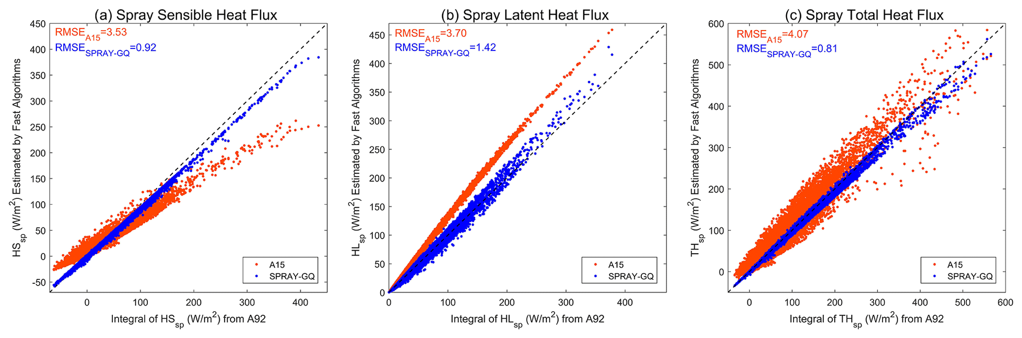
Based on the daily global WSP10, T02, 2 m dew point temperature, surface pressure and SWH of ERA5, the daily global OISST, and the ESA monthly global salinity, HS,SP and HL,SP from A15, SPRAY-GQ and A92 are calculated (Fig. 3). The computational time for SPRAY-GQ is about the same as that for A15 and about 36 times less than the time for A92. Compared with A92 (the dotted black line), A15 (red) overestimates HS,SP for low HS,SP (< 50 W m−2) and underestimates HS,SP for high HS,SP (> 50 W m−2) with a root mean square error (RMSE , is A15 value, yi is A92 value and n is the total number of grid points) of 3.40 W m−2 (Fig. 3a), while A15 shows consistent overestimations with a RMSE of 2.98 W m−2 for HL,SP (Fig. 3b). Overall, the RMSE of A15 is about 2.69 W m−2 for sea-spray-mediated total heat flux (; Fig. 3c). Andreas et al. (2015) derived A15 from A92 using single-radius droplets as bellwethers and wind functions, and extrapolated the wind functions at high wind speeds > 25 m s−1. Since the wind speeds in the study are less than 25 m s−1 (Fig. S1), the large difference between A15 and A92 is mainly due to the use of single-radius droplets. Compared with A15, SPRAY-GQ (blue) has less deviation from A92 for both HS,SP and HL,SP (Fig. 3a and b). The corresponding RMSEs of SPRAY-GQ for HS,SP, HL,SP and THSP are 0.83, 0.92 and 0.62 W m−2, all significantly lower (P<0.05 in Student's t test) than those of A15.
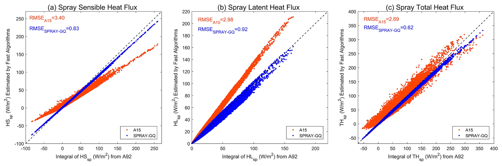
Figure 3Scatterplots of HS,SP (a), HL,SP (b) and total heat flux (c) estimated by fast algorithms (y axis) vs. those estimated by spectral integral in microphysical parameterization (x axis). The dotted black line is y=x. The corresponding RMSEs are marked in the upper left corner.
To test the robustness of the results, we also use WSP10, T02 and SPH of the OAFlux dataset to estimate HS,SP and HL,SP. As shown in Fig. 4, SPRAY-GQ has significantly (P<0.05 in Student's t test) lower deviations and RMSEs than A15, consistent with Fig. 3. Note that the values of HS,SP and HL,SP in Fig. 4 are larger than those in Fig. 3. This is because OAFlux only provides neutral wind speeds, calculated from wind stress and the corresponding roughness by assuming air is neutrally stratified. The neutral winds from OAFlux are larger than winds in ERA5, as indicated by previous studies (Lindemann et al., 2021; Seethala et al., 2021).
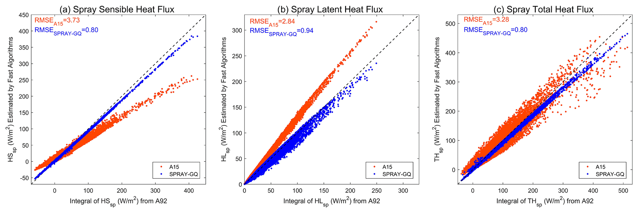
Figure 4The same as Fig. 3, but WSP10, 2 m air temperature and 2 m specific humidity of OAFlux are used.
In addition, since it is common to derive SWH from empirical equations (e.g., Andreas et al., 2008, 2015; Andreas and Decosmo, 2002; Andreas, 1992), we also use SWH generated by empirical equations of WSP10 (Andreas, 1992) instead of ERA5 SWH to estimate HS,SP and HL,SP (Fig. 5). Again, the RMSEs decrease significantly (P<0.05 in Student's t test) in SPRAY-GQ compared to A15, though the RMSEs become higher for all estimates due to the enhanced biases of SWH. The difference between SPRAY-GQ and A92 is always smaller than that between A15 and A92. Next, we will evaluate and compare the two fast algorithms in an atmosphere–ocean–wave coupled system (CFSv2.0-WW3).
4.2 Comparison in the CFSv2.0-WW3 coupling system
To compare the computational time of different parameterizations in the large-scale modeling system, the run time of the fully coupled experiments for 7 d forecast is given in Table 1 as an example. It is shown that the run time is about the same for SPRAY-GQ and SPRAY-A15. Both experiments run about 17 times faster than SPRAY-A92.
To illustrate the numerical errors of the two fast algorithms discussed in the context of the coupled system, comparisons are made for simulated SSTs, WSP10s and SWHs against OISST and ERA5 reanalysis. The results in the first 3 d are excluded in the comparison, since the wave influences are weak at the beginning of the simulations. Overall, the WSP10s of simulations are generally in the range of 0–25 m s−1 globally. At middle to high latitudes, the WSP10s generally exceed 10 m s−1 (Figs. S2 and S3 of the Supplement), at which the effects of sea spray can become significant (Andreas et al., 2015, 2008).
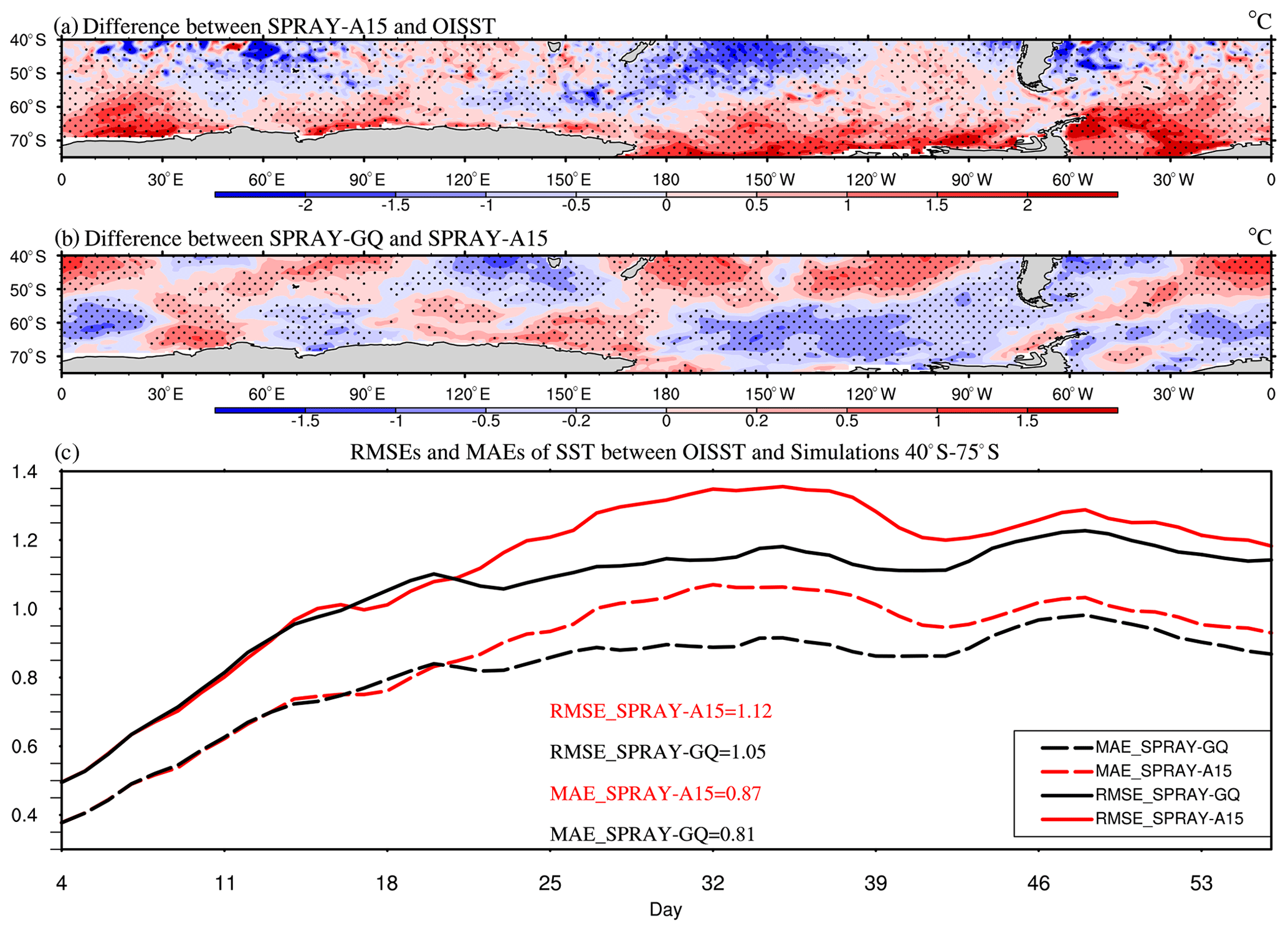
Figure 6The 53 d average SST (∘C) differences between SPRAY-A15 and OISST (a; SPRAY-A15 minus OISST), the differences between SPRAY-GQ and SPRAY-A15 (b; SPRAY-GQ minus SPRAY-A15), and the time series of domain-averaged RMSE and MAE (c; 0–360∘ E, 40–75∘ S) in January–February 2017. The first 3 d simulation is discarded. The dotted areas are statistically significant at 95 % confidence level.
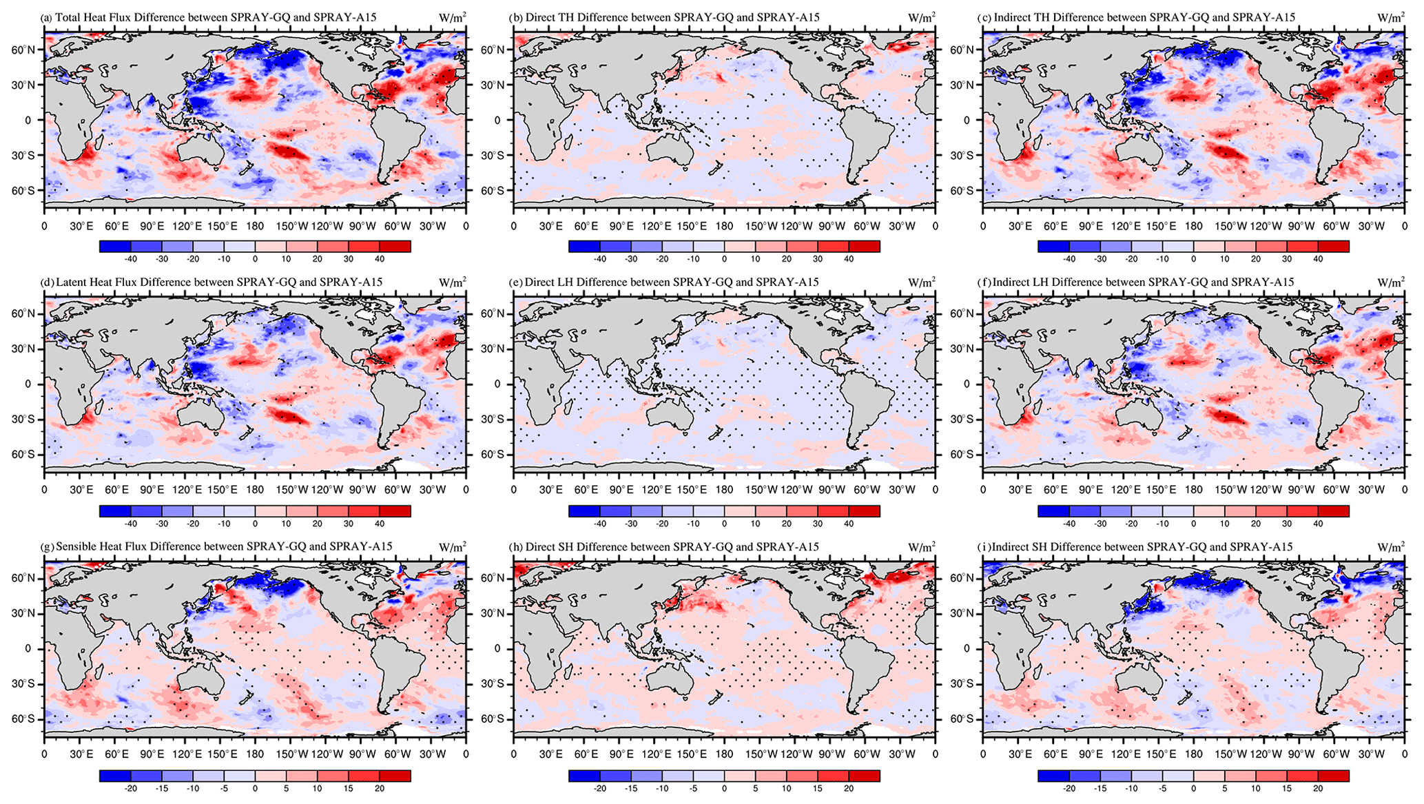
Figure 7The 53 d average differences of total heat flux (a–c), latent heat flux (d–f), and sensible heat flux (g–i) between SPRAY-GQ and SPRAY-A15 (SPRAY-GQ minus SPRAY-A15) in January–February 2017. The direct differences indicate sea-spray-mediated heat flux differences (b, e, h), and the indirect differences indicate interfacial (bulk) heat flux differences resulting from sea spray (c, f, i). The dotted areas are statistically significant at 95 % confidence level. A positive value of flux indicates an upward direction.
4.2.1 Sea surface temperature (SST)
In the austral summer, compared with OISST, large SST biases (> 1 ∘C or ∘C) of SPRAY-A15 occur in the Southern Hemisphere (SH; Fig. S4a in the Supplement), especially in the Southern Ocean. It is always a challenge to reduce the large SST biases in the Southern Ocean for climate models (e.g., Alessandro et al., 2019; Wang et al., 2014; Li et al., 2013; Bodas-Salcedo et al., 2012; Ceppi et al., 2012). In Fig. 6a, SSTs north (south) of 50∘ S in experiment SPRAY-A15 are mainly underestimated (overestimated). The domain-averaged RMSE (0–360∘ E, 40–75∘ S) in experiment SPRAY-A15 increases in the first month and then levels off (solid red line in Fig. 6c), while the domain-averaged RMSE in experiment SPRAY-GQ levels off about a week earlier (solid black line in Fig. 6c). The mean RMSE in SPRAY-GQ is significantly lower than that in SPRAY-A15 (P<0.05 in Student's t test). The increased (decreased) SSTs north (south) of 50∘ S in SPRAY-GQ compared to those in SPRAY-A15 (Fig. 6b) reduce the RMSE of SST in SPRAY-GQ. We also calculate the mean absolute error, MAE , where is simulated value, yi is OISST data and n is the total number of grid points. The MAEs are consistent with RMSEs (dotted line in Fig. 6c). Furthermore, the mean errors, ME (Fig. S5a in the Supplement), are smaller in SPRAY-GQ than SPRAY-A15.
To understand the effects of sea spray droplets on SST, we calculate the total heat flux (TH differences between SPRAY-GQ and SPRAY-A15 (Fig. 7a). The TH differences are significantly correlated with SST differences (Fig. S4b in the Supplement), with the spatial correlation coefficient of −0.41 (P<0.05 in Student's t test). We further decompose direct and indirect effects of sea spray droplets on heat fluxes following Song et al. (2022). The direct effect (HS,SP and HL,SP) is induced directly by sea spray droplets, calculated from A15 (Eqs. B1–B4 of Appendix B) and SPRAY-GQ (Sect. 3.1). The indirect effect (HS and HL) is the heat flux variation induced by changes of atmosphere and ocean variables (including wind, pressure, humidity and temperature) caused by direct effect, estimated by subtracting HS,SP and HL,SP from the output heat fluxes (HS,T and HL,T) of experiment SPRAY-A15 and SPRAY-GQ.
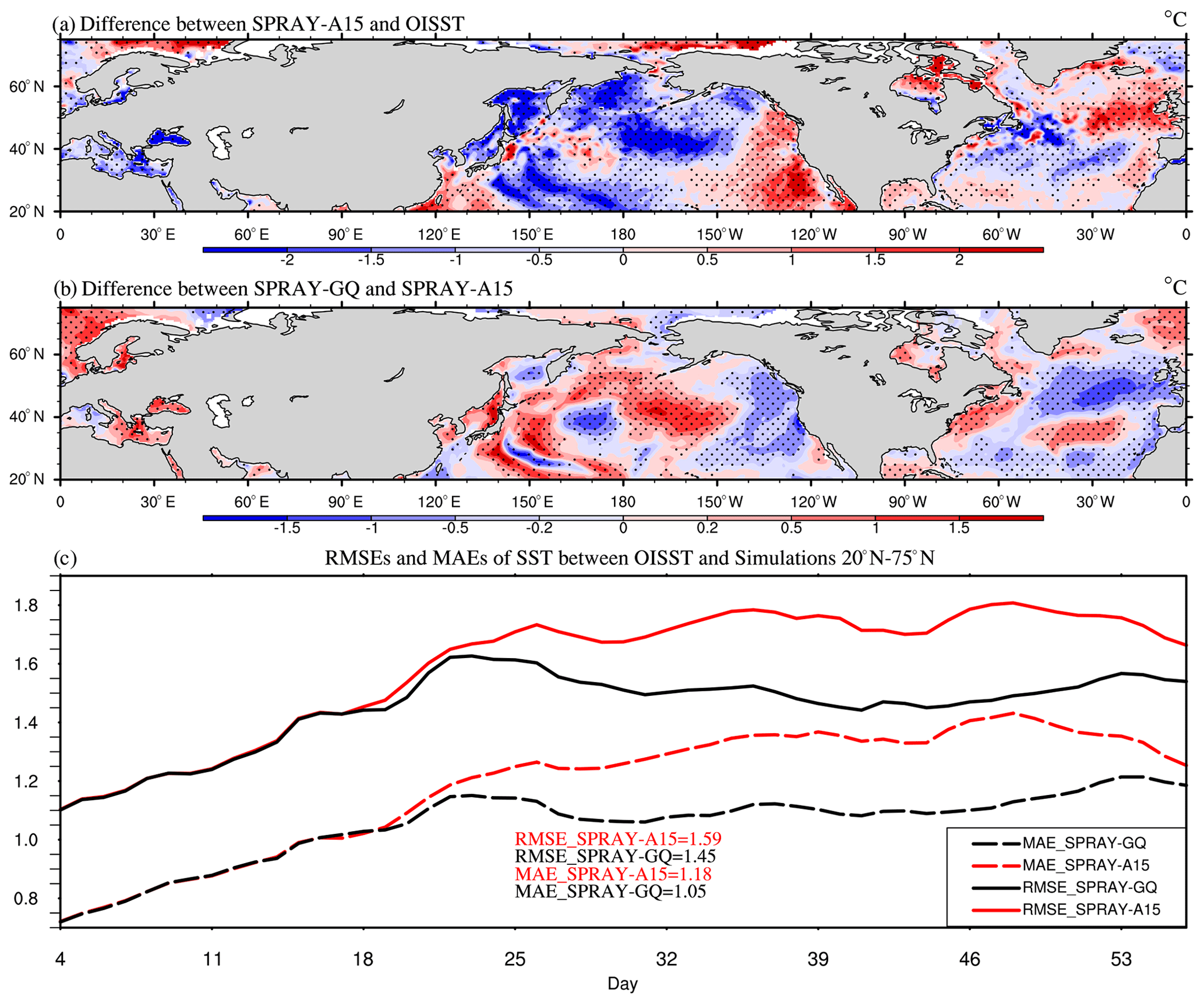
Figure 8The same as Fig. 6, but for August–September 2018 in 0–360∘ E, 20–75∘ N.
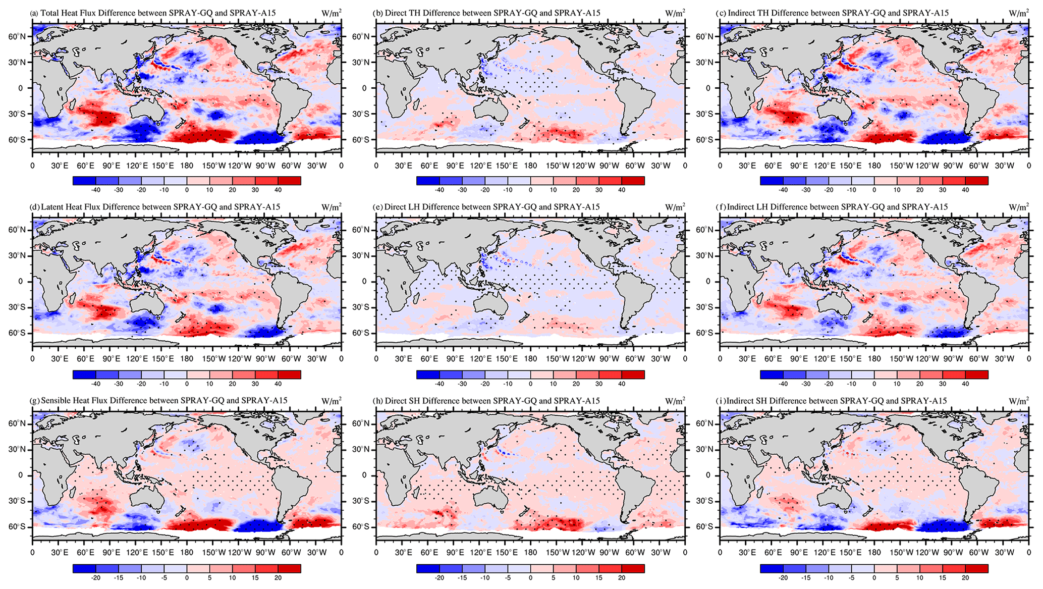
Figure 9The same as Fig. 7, but for August–September 2018.
In the Southern Ocean, although direct differences of HS,SP and HL,SP are relatively small (< 10 W m−2, Fig. 7b, e and h), the resulting changes of temperature and humidity lead to relatively large differences in indirect effects of HS and HL (Fig. 7c, f and i). Enhanced (reduced) THSP from ocean to atmosphere in the summer leads to increased (decreased) air–sea temperature difference and thus enhances (weakens) HS. Meanwhile the warmer (cooler) air also causes more (less) evaporation and thus more (less) HL. Finally, the enhanced (reduced) TH cools (warms) SST.

Figure 10The 53 d average WSP10 (m s−1) differences between SPRAY-A15 and ERA5 (a; SPRAY-A15 minus ERA5), the differences between SPRAY-GQ and SPRAY-A15 (b; SPRAY-GQ minus SPRAY-A15), and the time series of domain-averaged RMSE and MAE (c; 0–360∘ E, 0–60∘ N) in January–February 2017. The first 3 d simulation is discarded. The dotted areas are statistically significant at 95 % confidence level.
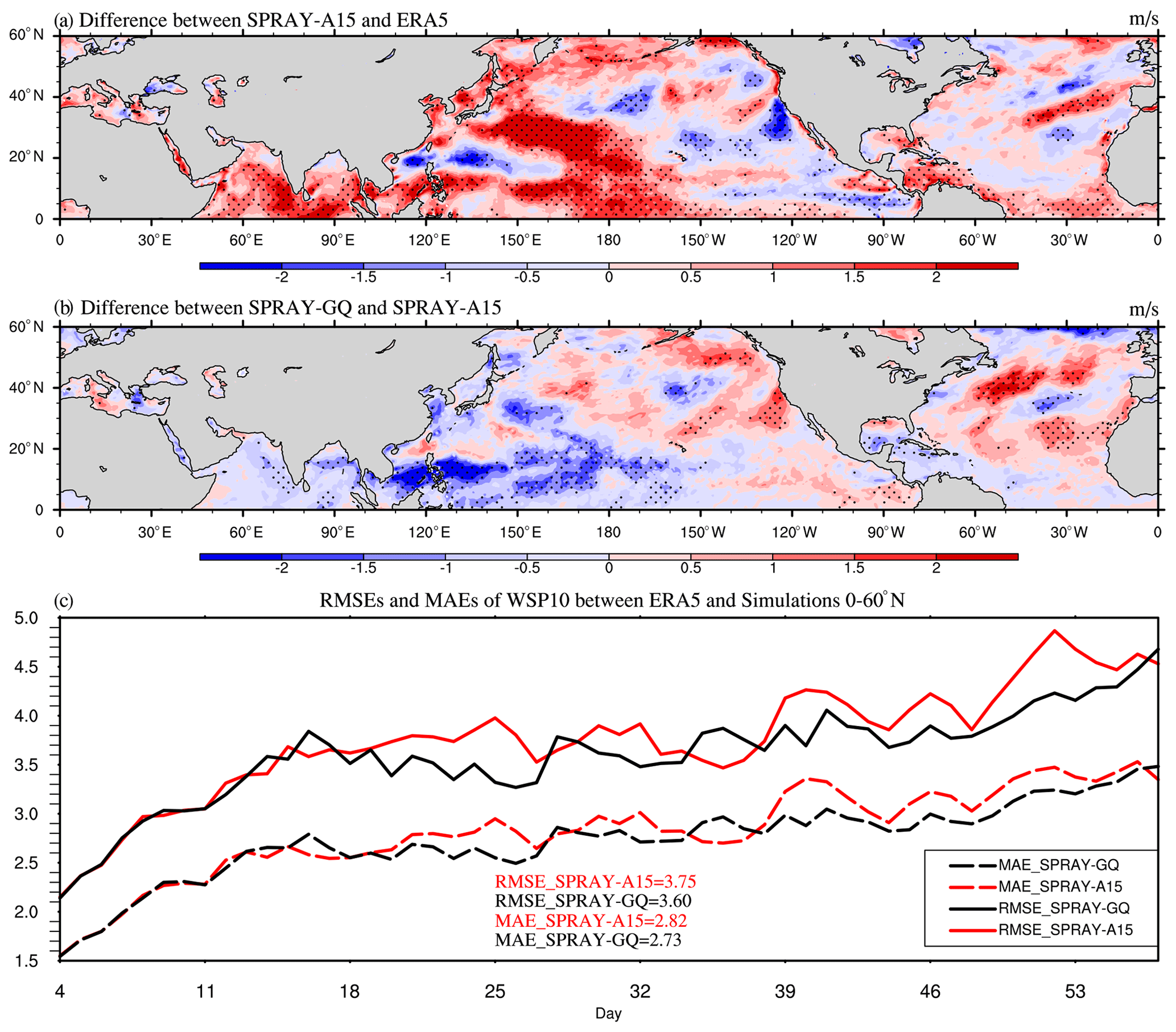
Figure 11The same as Fig. 10, but for August–September 2018.
In the boreal summer, large SST biases (> 1 ∘C or ∘C) of SPRAY-A15 mainly occur at middle to high latitudes of the Northern Hemisphere (NH; Fig. S6a in Supplement). Significant underestimations occur in the western and northern part of the North Pacific and at mid-latitudes of the North Atlantic, while large positive SST biases mainly occur in the eastern part of the North Pacific and at high latitudes of the North Atlantic (Fig. 8a). In experiment SPRAY-GQ, SSTs are warmer (cooler) in the previously underestimated (overestimated) regions (Fig. 8b). Therefore, the domain-averaged RMSE and MAE (0–360∘ E, 20–75∘ N) in SPRAY-GQ are significantly lower (P<0.01 in Student's t test) than in SPRAY-A15 after the first 3 weeks (Fig. 8c). Compared to SPRAY-A15, the overall underestimation is reduced in SPRAY-GQ (Fig. S5b). The spatial correlation coefficient between TH differences and SST differences (Figs. 9a, S6b) is −0.32 (P<0.05 in Student's t test). Consistent with the austral summer, the SST changes are related to the changes of heat flux (Fig. 9). The indirect effects of latent heat flux (Fig. 9f) play a major role in TH differences, which are modified by the direct effects (Fig. 9b, e and h). In addition, the changes of surface winds also contribute to the changes of SST. The reduced winds weaken the upper ocean mixing, the water becomes more stratified, and then the SST tends to be warmer and vice versa (Figs. S7 and S8).
4.2.2 Significant wave height (SWH) and 10 m wind speed (WSP10)
Compared with experiment SPRAY-A15, significant differences of WSP10 in SPRAY-GQ occur at middle to low latitudes of the NH (0–360∘ E, 0–60∘ N) in both winter and summer (Figs. S7b and S8b). As we know, satellite scatterometer and altimeter data are usually used to validate WSP10 and SWH for short-term weather forecast (e.g., Accadia et al., 2007; Djurdjevic and Rajkovic, 2008; Myslenkov et al., 2021). However, due to the spatial and temporal coverage of satellite data, we can only obtain the monthly averaged satellite data for the globe. Therefore, we compare the monthly averaged WSP10 and SWH from simulations with the corresponding satellite data (Figs. S9–S12). The comparison results (Figs. S9a and c–S12a and c) are consistent with those compared with ERA5 (Figs. S9b and d–S12b and d). From Figs. S9e–S12e, the differences of WSP10s between ERA5 and the satellite data are always less than 1 m s−1, and the differences of SWHs are always less than 0.3 m. Since ERA5 provides daily data for comparison, we will use ERA5 for validation in the following.
The ME of WSP10 (SPRAY-A15 minus ERA5) is 0.28 and 0.47 m s−1 in winter and summer (red in Fig. S5c and d), respectively, mainly due to the overestimations over the Pacific and the Atlantic Ocean (red in Figs. 10a and 11a), whereas in SPRAY-GQ the ME (SPRAY-GQ minus ERA5) is 0.15 and 0.33 m s−1 in winter and summer, respectively (black in Fig. S5c and d). The domain-averaged RMSEs and MAEs of WSP10s increase with time in the first 2 weeks and then gradually level off (Figs. 10c and 11c). The differences of WSP10 RMSEs and MAEs between SPRAY-GQ (black) and SPRAY-A15 (red) are very small in the first 2 weeks. Afterwards, the mean values of RMSE and MAE in SPRAY-GQ are significantly lower than those in SPRAY-A15, at 95 % confidence level in both boreal winter (Fig. 10c) and boreal summer (Fig. 11c).
The simulated SWHs changes are closely related to the changes of WSP10s (Shi et al., 2022). Therefore, the differences of SWHs (Figs. 12 and 13) are consistent with those of WSP10s (Figs. 10 and 11), with overestimated (underestimated) WSP10s corresponding to overestimated (underestimated) SWHs compared with ERA5. The SWHs in SPRAY-GQ are significantly different from those in SPRAY-A15 (Figs. 12b and 13b). In winter (summer), the SWH RMSE averages for SPRAY-A15 and SPRAY-GQ are 1.31 m (0.98 m) and 1.23 m (0.87 m), and after the first 2 weeks the RMSE and MAE in SPRAY-GQ are significantly lower than those in SPRAY-A15 at 95 % confidence level in both winter (Fig. 12c) and summer (Fig. 13c).

Figure 12The 53 d average SWH (m) differences between SPRAY-A15 and ERA5 (a; SPRAY-A15 minus ERA5), the differences between SPRAY-GQ and SPRAY-A15 (b; SPRAY-GQ minus SPRAY-A15), and the time series of domain-averaged RMSE and MAE (c; 0–360∘ E, 0–60∘ N) in January–February 2017. The first 3 d simulation is discarded. The dotted areas are statistically significant at 95 % confidence level.
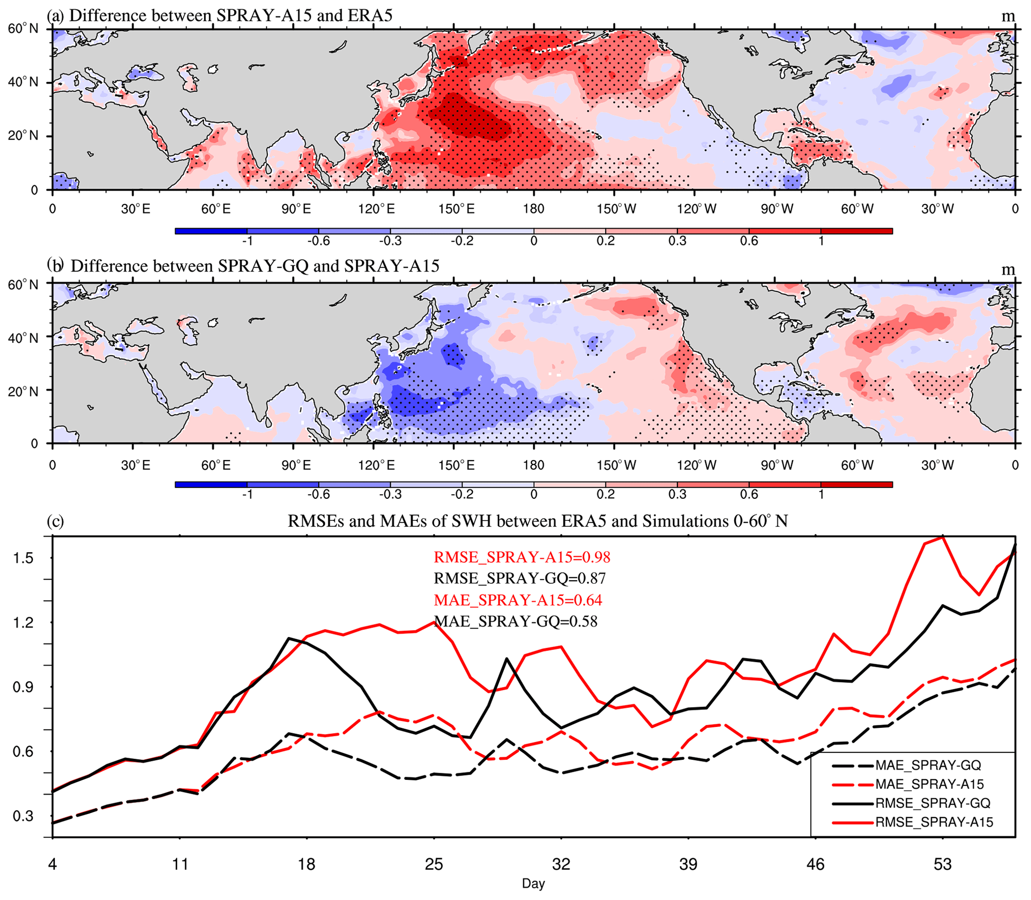
Figure 13The same as Fig. 12, but for August–September 2018.
The direct and indirect effects of sea spray droplets on heat fluxes can influence estimates of WSP10 and then SWH. The changes of WSP10s are related to the direct effects (HS,SP and HL,SP; Fig. 7b, e and h; Fig. 9b, e and h). The spatial correlation coefficients between WSP10 differences (Figs. S7b and S8b) and THSP differences (Figs. 7b and 9b) are 0.51 and 0.69 (P<0.01 in Student's t test) in winter and summer, respectively, because THSP differences can influence the sea level pressure (SLP) distribution (Figs. S15 and S16) and subsequently surface winds. For example, compared with SPRAY-A15, the decreased THSP of SPRAY-GQ in the Northwest Pacific in summer (Fig. 9b) leads to higher SLP and a smaller pressure gradient (Fig. S16) and thus decreased WSP10 (Fig. 11b), while the increased THSP in the Gulf of Alaska (Fig. 9b) leads to lower SLP and larger pressure gradient (Fig. S16) and thus enhanced WSP10 (Fig. 11b). The accelerated (decelerated) WSP10s further result in increased (decreased) interfacial heat transport (HS, HL) and increased (decreased) SWHs.
Based on a GQ method, we develop a new fast algorithm based on Andreas's (1989, 1990, 1992) full-size microphysical parameterization (A92) for sea-spray-mediated heat fluxes. Using global satellite measurements and reanalysis data, we found that the difference between SPRAY-GQ and A92 is significantly smaller than that between A15 and A92 (Andreas et al., 2015). To evaluate the numerical error of the SPRAY-GQ/A15 fast algorithm, we implement them in the two-way coupled CFSv2.0-WW3 system. A series of 56 d simulations from 3 January to 28 February 2017 and from 3 August to 28 September 2018 are conducted. The results are compared against satellite measurements and ERA5 reanalysis. The comparison shows that the sea-spray-mediated heat flux in SPRAY-GQ can reasonably modulate total heat flux compared with SPRAY-A15 and significantly reduce the SST biases in the Southern Ocean (middle to high latitudes of the NH) for the austral (boreal) summer and WSP10 and SWH after the first 2 weeks at middle to low latitudes of the NH for both boreal winter and summer. Overall, our fast algorithm based on GQ is applicable to sea-spray-mediated heat flux parameterization in coupled models.
To investigate the effects of spray-mediated heat flux on simulations, two 56 d experiments without sea spray effect (CTRL) in boreal winter and summer are conducted, respectively, and the differences of simulated SST, WSP10, SWH, T02 and SPH between SPRAY-GQ and CTRL are compared in Figs. S17–S21 in the Supplement. The introduction of sea spray cannot significantly reduce the global overall errors of simulations, but it leads to regional improvements (blue in Figs. S17e and f–S21e and f). For example, compared with CTRL in January–February 2017, SST MAE of SPRAY-GQ in the southeast of Australia decreases (Fig. S17e) because of warmer SST (Fig. S17c) related to reduced wind (Fig. S18c). The reduced wind here also leads to lower SWH (Fig. S19c) and thus reduced SWH overestimation (Fig. S19e). Meanwhile, SPRAY-GQ reduces MAE of T02 and SPH (Figs. S20e and S21e) by increasing temperature and moisture (Figs. S20c and S21c). The reduced errors are related to the relatively large WSP10s over the areas (Figs. S2 and S3), since the effects of sea spray become important at wind speeds larger than 10 m s−1.
In addition to the variables aforementioned, the changes of simulated cloud fraction were also compared. However, the effects of sea-spray-mediated heat flux on cloud fraction are non-significant for the 2-month simulation, so the results are not shown. Besides this, the lack of other processes related to sea spray may be one of the reasons why the global overall error cannot be reduced effectively. For example, for simulated WSP10 and SWH in SPRAY-GQ, the significant overestimations in the SH still exist especially in August–September 2018 (Figs. S18 and S19 in the Supplement). As Andreas (2004) indicated, sea spray droplets also influence the surface momentum flux by injecting more momentum into the ocean from the atmosphere, which might further decrease the surface wind speed. We will consider this process in a future study.
Sea-spray-mediated heat fluxes are related to the sea spray generation function (SSGF). Based on a number of laboratory and field observations, varieties of SSGF were derived (e.g., Koga, 1981; Monahan et al., 1982; Troitskaya et al., 2018; Andreas, 1992, 1998, 2002; Fairall et al., 1994; Veron, 2015), whereas their differences can reach six orders of magnitude (Andreas, 1998). There is currently no consensus on the most suitable choice. In this study, we use SSGF of Fairall et al. (1994), recommended by Andreas (2002), to get a mean bias of 3.70 and 0.095 W m−2 for latent and sensible heat flux, respectively (Andreas et al., 2015), consistent with recent observations of Xu et al. (2021b). However, the improved SST and other variables cannot be reliably assigned to the usage of the GQ method, due to the uncertainties of the coupled model itself and SSGF.
When wind speed is larger than 10 m s−1, spray-mediated heat flux can become as important as the interfacial heat flux (Andreas and Decosmo, 1999, 2002). Particularly, even in the absence of air–sea temperature difference, the spray-mediated sensible heat flux is still present (Andreas et al., 2008). As indicated by previous studies (e.g., Garg et al., 2018; Song et al. 2022), it is necessary to superimpose the spray-mediated heat flux on the bulk formula to complete the physics of turbulent heat transfer for coupled simulation. Since the full microphysical parameterization (A92) is computationally expensive, an efficient algorithm that captures the main features of A92 can be beneficial to large-scale climate systems or operational storm models. The GQ method proposed in the study can efficiently calculate the spray-mediated heat flux and agrees better with A92 than A15. Therefore, the GQ-based spray-mediated heat flux is promising for wide applications in large-scale climate systems and operational storm models.
Based on the cloud microphysical parameterization of Pruppacher and Klett (1978), Andreas (1989, 1990, 1992) proposed a parameterization of sea-spray-related heat fluxes for droplets with different radius, from formation at sea surface to equilibrium with environment; that is,
Here, QS and QL are sensible heat flux and latent heat flux resulting from sea spray droplets with initial radius r0, ρw is the sea water density, Cps is the specific heat, Lv is the latent heat of vaporization of water, Tw is the water temperature, Teq is the temperature of droplet when it reaches thermal equilibrium with ambient condition, req is the radius of droplet when it reaches moisture equilibrium with ambient condition, τf is the residence time for droplets in the atmosphere, r(τf) is the corresponding radius, τT is the characteristic e folding time of droplet temperature, and τr is the characteristic e folding time of droplet radius. The detailed calculation of these microphysical quantities can be found in Andreas (1989, 1990, 1992). is the sea spray generation function, which represents the produced number of droplets with initial radius r0 (Andreas, 1992). For this term, the function of Fairall et al. (1994) was recommended by Andreas (2002). According to the review in Andreas (2002), the of Fairall et al. (1994) is related on that of Andreas (1992) as
Here, U10 is the 10 m wind and .
The total sea spray fluxes are obtained by integrating QS and QL corresponding to all r0. Based on Andreas (1990), the lower and upper limits of r0 are 2 and 500 µm, respectively; that is,
Note that and are nominal sea spray fluxes but not the actual HS,SP and HL,SP (Andreas and Decosmo, 1999, 2002), because there are interactions between these two terms and the microphysical functions also lead to uncertainties (Fairall et al., 1994). Therefore, and are tuned by non-negative constants α, β and γ (Andreas and Decosmo, 2002; Andreas et al., 2008, 2015; Andreas, 2003) as
In Eq. (A8), the α term indicates the sea-spray-mediated latent heat flux from the top of DEL to atmosphere. Because the evaporation of droplets absorbs heat, which is provided by sea-spray-mediated sensible heat (Fairall et al., 1994), the negative α term appears in Eq. (A7). The evaporation also cools DEL and thus increases the air–sea temperature difference: therefore it contributes to a positive γ term in Eq. (A7). Different values of α, β and γ were given in Andreas and Decosmo (2002), Andreas (2003), and Andreas et al. (2008, 2015) to minimize the bias between estimations and observations of turbulent heat fluxes measured by eddy correlation. And Andreas et al. (2015) validated the most observation data, which are 4000 sets, to derive .
Andreas (2003) and Andreas et al. (2008, 2015) developed a fast algorithm to approximate HS,SP and HL,SP by a characteristic radius; that is,
Here, Teq,100 is Teq of droplets with r0=100 µm, τf,50 is τf of droplets with r0=50 µm, and Vs and VL are functions of the bulk friction velocity u∗. As indicated by Andreas et al. (2008, 2015), the characteristic radiuses of 100 µm and 50 µm for sensible and latent heat fluxes are chosen, respectively, because QS and QL show a large peak in the vicinity of these values (Fig. 1). Vs and VL are calculated in Andreas et al. (2015) as
GQ is a method to approximate the definite integral of a function f(x) via the function values at a small number of specified nodes (Gauss, 1815; Jacobi, 1826). In this study we use the form of n-node Gauss–Legendre quadrature on as
Here, xi is the specified node, and ωi is the corresponding weight. For n=3, , x2=0, x3=0.775, , ω2=0.889.
For a function g(ξ) on [a, b], Eq. (C1) can be transformed to
The sea spray code can be found at https://doi.org/10.5281/zenodo.7100345 or https://zenodo.org/record/7100345#.Y66vRtVByHt (Shi and Xu, 2022). The code for the CFSv2.0-WW3 system can be found at https://doi.org/10.5281/zenodo.5811002 (Shi et al., 2021) including the coupling, preprocessing, run control and postprocessing scripts. The initial fields for CFSv2.0 are generated by the real-time operational Climate Data Assimilation System, downloaded from the CFSv2.0 official website (http://nomads.ncep.noaa.gov/pub/data/nccf/com/cfs/prod, NOAA, 2023). The daily average satellite Optimum Interpolation SST (OISST) data are obtained from NOAA (https://www.ncdc.noaa.gov/oisst, National Centers for Environmental Information, 2023). The fifth-generation European Centre for Medium-range Weather Forecasts (ECMWF) Reanalysis (ERA5) are available at the Copernicus Climate Change Service (C3S) Climate Date Store (https://doi.org/10.24381/cds.adbb2d47, Hersbach et al., 2018). The daily Objectively Analyzed air–sea Fluxes (OAFlux) products are available at https://oaflux.whoi.edu/heat-flux (Woods Hole Oceanographic Institution, 2023). The global monthly mean salinity observations of the European Space Agency (ESA) are from https://doi.org/10.5285/5920a2c77e3c45339477acd31ce62c3c (Boutin et al., 2020). The monthly global ocean RSS Satellite Data Products for 10 m wind speed are from https://data.remss.com/wind/monthly_1deg/ (Remote Sensing Systems, 2023), and the Reprocessed L4 Satellite Measurements for significant wave height are from https://doi.org/10.48670/moi-00177 (Collecte Localisation Satellites, 2021).
The supplement related to this article is available online at: https://doi.org/10.5194/gmd-16-1839-2023-supplement.
FX and RS designed the experiments and RS carried them out. RS developed the code of coupling parametrizations and produced the figures. RS prepared the paper with contributions from all co-authors. FX contributed to review and editing.
The contact author has declared that neither of the authors has any competing interests.
Publisher's note: Copernicus Publications remains neutral with regard to jurisdictional claims in published maps and institutional affiliations.
The authors are grateful to Jiangnan Li for help with the GQ codes. We also thank the two anonymous reviewers and the handling editor for their constructive comments.
This research has been supported by the National Key Research and Development Program of China (grant nos. 2020YFA0607900 and 2021YFC3101601) and the National Natural Science Foundation of China (grant no. 42176019).
This paper was edited by Qiang Wang and reviewed by two anonymous referees.
Accadia, C., Zecchetto, S., Lavagnini, A., and Speranza, A.: Comparison of 10-m wind forecasts from a regional area model and QuikSCAT scatterometer wind observations over the Mediterranean Sea, Mon. Weather Rev., 135, 1945–1960, 2007.
Alessandro, J. D., Diao, M., Wu, C., Liu, X., Jensen, J. B., and Stephens, B. B.: Cloud phase and relative humidity distributions over the Southern Ocean in austral summer based on in situ observations and CAM5 simulations, J. Climate, 32, 2781–2805, 2019.
Andreas, E. L.: Thermal and size evolution of sea spray droplets, Cold Regions Research and Engineering Laboratory (U.S.), Engineer Research and Development Center (U.S.), CRREL report 89-11, http://hdl.handle.net/11681/9057, 1989.
Andreas, E. L.: Time constants for the evolution of sea spray droplets, Tellus B., 42, 481–497, 1990.
Andreas, E. L.: Sea spray and the turbulent air-sea heat fluxes, J. Geophys. Res.-Oceans., 97, 11429–11441, 1992.
Andreas, E. L.: A new sea spray generation function for wind speeds up to 32 ms- 1, J. Phys. Oceanogr., 28, 2175–2184, 1998.
Andreas, E. L.: A review of the sea spray generation function for the open ocean, Adv. Fluid. Mech. Ser., 33, 1–46, 2002.
Andreas, E. L.: 3.4 An Algorithm to Predict the Turbulent Air-Sea Fluxes in High-Wind, Spray Conditions, Environmental Science, https://ams.confex.com/ams/pdfpapers/52221.pdf (last access: 18 March 2023), 2003.
Andreas, E. L.: Spray stress revisited, J. Phys. Oceanogr., 34, 1429–1440, 2004.
Andreas, E. L.: Spray-mediated enthalpy flux to the atmosphere and salt flux to the ocean in high winds, J. Phys. Oceanogr., 40, 608–619, 2010.
Andreas, E. L. and Decosmo, J.: Sea spray production and influence on air-sea heat and moisture fluxes over the open ocean, in: Air-sea exchange: physics, chemistry and dynamics, Springer, 327–362, https://doi.org/10.1007/978-94-015-9291-8_13, 1999.
Andreas, E. L. and Decosmo, J.: The signature of sea spray in the HEXOS turbulent heat flux data, Bound-Lay. Meteorol., 103, 303–333, 2002.
Andreas, E. L. and Emanuel, K. A.: Effects of sea spray on tropical cyclone intensity, J. Atmos. Sci., 58, 3741–3751, 2001.
Andreas, E. L., Mahrt, L., and Vickers, D.: An improved bulk air–sea surface flux algorithm, including spray-mediated transfer, Q. J. Roy. Meteor. Soc., 141, 642–654, 2015.
Andreas, E. L., Persson, P. O. G., and Hare, J. E.: A bulk turbulent air–sea flux algorithm for high-wind, spray conditions, J. Phys. Oceanogr., 38, 1581–1596, 2008.
Andreas, E. L., Edson, J. B., Monahan, E. C., Rouault, M. P., and Smith, S. D.: The spray contribution to net evaporation from the sea: A review of recent progress, Bound-Lay. Meteorol., 72, 3–52, 1995.
Bao, Y., Song, Z., and Qiao, F.: FIO-ESM version 2.0: Model description and evaluation, J. Geophys. Res.-Oceans., 125, e2019JC016036, https://doi.org/10.1029/2019JC016036, 2020.
Bodas-Salcedo, A., Williams, K., Field, P., and Lock, A.: The surface downwelling solar radiation surplus over the Southern Ocean in the Met Office model: The role of midlatitude cyclone clouds, J. Climate., 25, 7467–7486, 2012.
Borisenkov, E.: Some mechanisms of atmosphere-ocean interaction under stormy weather conditions, Probl. Arct. Antarct., 43, 73–83, 1974.
Bortkovskii, R.: On the mechanism of interaction between the ocean and the atmosphere during a storm, Fluid. Mech. Sov. Res., 2, 87–94, 1973.
Boutin, J., Vergely, J.-L., Reul, N., Catany, R., Koehler, J., Martin, A., Rouffi, F., Arias, M., Chakroun, M., Corato, G., Estella-Perez, V., Guimbard, S., Hasson, A., Josey, S., Khvorostyanov, D., Kolodziejczyk, N., Mignot, J., Olivier, L., Reverdin, G., Stammer, D., Supply, A., Thouvenin-Masson, C., Turiel, A., Vialard, J., Cipollini, P., and Donlon, C.: ESA Sea Surface Salinity Climate Change Initiative (Sea_Surface_Salinity_cci): Weekly sea surface salinity product, v03.21, for 2010 to 2020, NERC EDS Centre for Environmental Data Analysis, [data set], https://doi.org/10.5285/5920a2c77e3c45339477acd31ce62c3c, 2021.
Burk, S. D.: The generation, turbulent transfer and deposition of the sea-salt aerosol, J. Atmos. Sci., 41, 3040–3051, 1984.
Ceppi, P., Hwang, Y. T., Frierson, D. M., and Hartmann, D. L.: Southern Hemisphere jet latitude biases in CMIP5 models linked to shortwave cloud forcing, Geophys. Res. Lett., 39, L19708, https://doi.org/10.1029/2012GL053115, 2012.
Collecte Localisation Satellites: Global Ocean L4 Significant Wave Height From Reprocessed Satellite Measurements, Collecte Localisation Satellites [data set], https://doi.org/10.48670/moi-00177, 2021.
Djurdjevic, V. and Rajkovic, B.: Verification of a coupled atmosphere-ocean model using satellite observations over the Adriatic Sea, Ann. Geophys., 26, 1935–1954, https://doi.org/10.5194/angeo-26-1935-2008, 2008.
Edson, J. B. and Andreas, E. L.: Modeling the role of sea spray on air-sea heat and moisture exchange, Final Rep., 6, 18, https://citeseerx.ist.psu.edu/document?repid=rep1&type=pdf&doi=9dd59325684a16bf0d222200f806958ff0e35dd8#page=20 (last access: 18 March 2023), 1997.
Emanuel, K. A.: Sensitivity of tropical cyclones to surface exchange coefficients and a revised steady-state model incorporating eye dynamics, J. Atmos. Sci., 52, 3969–3976, 1995.
Fairall, C. and Larsen, S. E.: Dry deposition, surface production and dynamics of aerosols in the marine boundary layer, Atmos. Environ., 18, 69–77, 1984.
Fairall, C., Davidson, K., and Schacher, G.: An analysis of the surface production of sea-salt aerosols, Tellus B., 35, 31–39, 1983.
Fairall, C., Kepert, J., and Holland, G.: The effect of sea spray on surface energy transports over the ocean, Global Atmos. Ocean Syst., 2, 121–142, 1994.
Fairall, C., Bradley, E. F., Rogers, D. P., Edson, J. B., and Young, G. S.: Bulk parameterization of air-sea fluxes for tropical ocean-global atmosphere coupled-ocean atmosphere response experiment, J. Geophys. Res.-Oceans., 101, 3747–3764, 1996.
Fox-Kemper, B., Johnson, L., and Qiao, F.: Ocean near-surface layers, in: Ocean Mixing, Elsevier, 65–94, https://doi.org/10.1016/B978-0-12-821512-8.00011-6, 2022.
Garg, N., Ng, E. Y. K., and Narasimalu, S.: The effects of sea spray and atmosphere–wave coupling on air–sea exchange during a tropical cyclone, Atmos. Chem. Phys., 18, 6001–6021, https://doi.org/10.5194/acp-18-6001-2018, 2018.
Gauss, C. F.: Methodvs nova integralivm valores per approximationem inveniendi, apvd Henricvm Dieterich, https://books.google.de/books?id=OitfAAAAcAAJ&pg=PA1&hl=de&source=gbs_selected_pages&redir_esc=y#v=onepage&q&f=false (last access: 18 March 2023), 1815.
Griffies, S. M., Harrison, M. J., Pacanowski, R. C., and Rosati, A.: A technical guide to MOM4, GFDL Ocean Group Tech. Rep, 5, 342 pp., https://www.gfdl.noaa.gov/bibliography/related_files/smg0301.pdf (last access: 20 January 2022), 2004.
Hersbach, H., Bell, B., Berrisford, P., Biavati, G., Horányi, A., Muñoz Sabater, J., Nicolas, J., Peubey, C., Radu, R., Rozum, I., Schepers, D., Simmons, A., Soci, C., Dee, D., and Thépaut, J.-N.: ERA5 hourly data on single levels from 1979 to present, Copernicus Climate Change Service (C3S) Climate Data Store (CDS) [data set], https://doi.org/10.24381/cds.adbb2d47, 2018.
Hersbach, H., Bell, B., Berrisford, P., Hirahara, S., Horányi, A., Muñoz-Sabater, J., Nicolas, J., Peubey, C., Radu, R., and Schepers, D.: The ERA5 global reanalysis, Q. J. Roy. Meteor. Soc., 146, 1999–2049, 2020.
Jacobi, C. G. J.: Ueber Gauss neue Methode, die Werthe der Integrale näherungsweise zu finden, 301–308, https://doi.org/10.1515/crll.1826.1.301, 1826.
Kalnay, E., Kanamitsu, M., Kistler, R., Collins, W. D., Deaven, D. G., Gandin, L. S., Iredell, M. D., Saha, S., White, G. H., and Woollen, J.: The NCEP/NCAR 40-Year Reanalysis Project, B. Am. Meteorol. Soc., 77, 437–471, https://doi.org/10.1175/1520-0477(1996)077<0437:TNYRP>2.0.CO;2, 1996.
Koga, M.: Direct production of droplets from breaking wind-waves – its observation by a multi-colored overlapping exposure photographing technique, Tellus, 33, 552–563, 1981.
Lhuissier, H. and Villermaux, E.: Bursting bubble aerosols, J. Fluid. Mech., 696, 5–44, 2012.
Li, J., Waliser, D., Stephens, G., Lee, S., L'Ecuyer, T., Kato, S., Loeb, N., and Ma, H. Y.: Characterizing and understanding radiation budget biases in CMIP3/CMIP5 GCMs, contemporary GCM, and reanalysis, J. Geophys. Res.-Atmos., 118, 8166–8184, 2013.
Li, J. N. and Barker, H. W.: Computation of domain-average radiative flux profiles using Gaussian quadrature, Q. J. Roy. Meteor. Soc., 144, 720–734, 2018.
Lindemann, D., Avila-Diaz, A., Pezzi, L., Rodrigues, J., Freitas, R. A., Coelho, L., Alonso, M., and Cerón, W. L.: The Surface Wind Influence on the Heat Fluxes Variability on the South Atlantic, Research Square [preprint], https://doi.org/10.21203/rs.3.rs-235260/v1, 2021.
Ling, S. and Kao, T.: Parameterization of the moisture and heat transfer process over the ocean under whitecap sea states, J. Phys. Oceanogr., 6, 306–315, 1976.
Liu, B., Guan, C., Xie, L. a., and Zhao, D.: An investigation of the effects of wave state and sea spray on an idealized typhoon using an air-sea coupled modeling system, Adv. Atmos. Sci., 29, 391–406, 2012.
Liu, L., Zhang, C., Li, R., Wang, B., and Yang, G.: C-Coupler2: a flexible and user-friendly community coupler for model coupling and nesting, Geosci. Model Dev., 11, 3557–3586, https://doi.org/10.5194/gmd-11-3557-2018, 2018.
McClarren, R.: Gauss Quadrature and Multi-dimensional Integrals, Computational Nuclear Engineering and Radiological Science Using Python, Academic Press: Cambridge, MA, USA, 287–299, https://doi.org/10.1016/B978-0-12-812253-2.00018-2, 2018.
Melville, W. K.: The role of surface-wave breaking in air-sea interaction, Annu. Rev. Fluid Mech., 28, 279–321, https://doi.org/10.1146/annurev.fl.28.010196.001431, 1996.
Monahan, E. and Van Patten, M. A.: The climate and health implications of bubble-mediated sea-air exchange, https://repository.library.noaa.gov/view/noaa/39512 (last access: 18 March 2023), 1988.
Monahan, E., Davidson, K., and Spiel, D.: Whitecap aerosol productivity deduced from simulation tank measurements, J. Geophys. Res.-Oceans., 87, 8898–8904, 1982.
Myslenkov, S., Zelenko, A., Resnyanskii, Y., Arkhipkin, V., and Silvestrova, K.: Quality of the Wind Wave Forecast in the Black Sea Including Storm Wave Analysis, Sustainability-Basel, 13, 13099, https://doi.org/10.3390/su132313099, 2021.
National Centers for Environmental Information: Optimum Interpolation SST, National Centers for Environmental Information [data set], https://www.ncdc.noaa.gov/oisst, last access: 18 March 2023.
NOAA: CFSv2.0 Initial Fields, NOAA [data set], https://nomads.ncep.noaa.gov/pub/data/nccf/com/cfs/prod, last access: 18 March 2023.
Pruppacher, H. R. and Klett, J. D.: Microstructure of atmospheric clouds and precipitation, in: Microphysics of Clouds and Precipitation, Springer, 9–55, https://doi.org/10.1007/978-94-009-9905-3_2, 1978.
Remote Sensing Systems: Monthly merged global wind product, Remote Sensing Systems [data set], https://data.remss.com/wind/monthly_1deg/, last access: 18 March 2023.
Resch, F. and Afeti, G.: Film drop distributions from bubbles bursting in seawater, J. Geophys. Res.-Oceans., 96, 10681–10688, 1991.
Reynolds, R. W., Smith, T. M., Liu, C., Chelton, D. B., Casey, K. S., and Schlax, M. G.: Daily High-Resolution-Blended Analyses for Sea Surface Temperature, J. Climate., 20, 5473–5496, https://doi.org/10.1175/2007JCLI1824.1, 2007.
Saha, S., Moorthi, S., Wu, X., Wang, J., Nadiga, S., Tripp, P., Behringer, D., Hou, Y., Chuang, H., and Iredell, M. D.: The NCEP Climate Forecast System Version 2, J. Climate, 27, 2185–2208, https://doi.org/10.1175/JCLI-D-12-00823.1, 2014.
Seethala, C., Zuidema, P., Edson, J., Brunke, M., Chen, G., Li, X. Y., Painemal, D., Robinson, C., Shingler, T., and Shook, M.: On assessing ERA5 and MERRA2 representations of cold-air outbreaks across the Gulf Stream, Geophys. Res. Lett., 48, e2021GL094364, https://doi.org/10.1029/2021GL094364, 2021.
Shi, R. and Xu, F.: Codes for Sea Spray, Zenodo [code], https://doi.org/10.5281/zenodo.7100345, 2022.
Shi, R., Xu, F., Liu, L., Fan, Z., and Yu, H.: The Effects of Ocean Surface Waves on Global Forecast in CFS Modeling System v2.0, Zenodo [code], https://doi.org/10.5281/zenodo.5811002, 2021.
Shi, R., Xu, F., Liu, L., Fan, Z., Yu, H., Li, H., Li, X., and Zhang, Y.: The effects of ocean surface waves on global intraseasonal prediction: case studies with a coupled CFSv2.0–WW3 system, Geosci. Model Dev., 15, 2345–2363, https://doi.org/10.5194/gmd-15-2345-2022, 2022.
Smith, R. K.: On the theory of CISK, Q. J. Roy. Meteor. Soc., 123, 407–418, 1997.
Song, Y., Qiao, F., Liu, J., Shu, Q., Bao, Y., Wei, M., and Song, Z.: Effects of sea spray on large-scale climatic features over the Southern Ocean, J. Climate, 35, 4645–4663, https://doi.org/10.1175/JCLI-D-21-0608.1, 2022.
Spiel, D. E.: More on the births of jet drops from bubbles bursting on seawater surfaces, J. Geophys. Res.-Oceans., 102, 5815–5821, 1997.
Thorpe, S.: Bubble clouds and the dynamics of the upper ocean, Q. J. Roy. Meteor. Soc., 118, 1–22, 1992.
Troitskaya, Y., Kandaurov, A., Ermakova, O., Kozlov, D., Sergeev, D., and Zilitinkevich, S.: The “bag breakup” spume droplet generation mechanism at high winds. Part I: Spray generation function, J. Phys. Oceanogr., 48, 2167–2188, 2018.
Van Eijk, A., Kusmierczyk-Michulec, J., Francius, M., Tedeschi, G., Piazzola, J., Merritt, D., and Fontana, J.: Sea-spray aerosol particles generated in the surf zone, J. Geophys. Res.-Atmos., 116, D19210, https://doi.org/10.1029/2011JD015602, 2011.
Veron, F.: Ocean spray, Annu. Rev. Fluid. Mech., 47, 507–538, 2015.
Wang, C., Zhang, L., Lee, S.-K., Wu, L., and Mechoso, C. R.: A global perspective on CMIP5 climate model biases, Nat. Clim. Change, 4, 201–205, 2014.
WAVEWATCH III Development Group: User manual and system documentation of WAVEWATCH III version 5.16, NOAA/NWS/NCEP/MMAB Technical Note 329, 326, https://polar.ncep.noaa.gov/waves/wavewatch/manual.v5.16.pdf (last access: 20 January 2022), 2016.
Woods Hole Oceanographic Institution: Objectively Analyzed air-sea Fluxes (OAFlux) for the Global Oceans, Woods Hole Oceanographic Institution [data set], ftp://ftp.whoi.edu/pub/science/oaflux/data_v3, last access: 8 January 2023.
Wu, J.: Evaporation due to spray, J. Geophys. Res., 79, 4107–4109, 1974.
Wu, L., Cheng, X., Zeng, Q., Jin, J., Huang, J., and Feng, Y.: On the upward flux of sea-spray spume droplets in high-wind conditions, J. Geophys. Res.-Atmos., 122, 5976–5987, 2017.
Xu, X., Voermans, J., Ma, H., Guan, C., and Babanin, A. V.: A Wind–Wave-Dependent Sea Spray Volume Flux Model Based on Field Experiments, Journal of Marine Science and Engineering, 9, 1168, https://doi.org/10.3390/jmse9111168, 2021a.
Xu, X., Voermans, J., Liu, Q., Moon, I.-J., Guan, C., and Babanin, A.: Impacts of the Wave-Dependent Sea Spray Parameterizations on Air–Sea–Wave Coupled Modeling under an Idealized Tropical Cyclone, Journal of Marine Science and Engineering, 9, 1390, https://doi.org/10.3390/jmse9121390, 2021b.
Yu, L., Jin, X., and Weller, R. A.: Multidecade global flux datasets from the Objectively Analyzed Air-Sea Fluxes (OAFlux) Project: Latent and sensible heat fluxes, ocean evaporation, and related surface meteorological variables, Woods Hole Oceanographic Institution OAFlux Project Tec. [data set], Rep., ftp://ftp.whoi.edu/pub/science/oaflux/data_v3/OAFlux_TechReport_3rd_release.pdf (last access: 2 January 2023), 2008.
Zhao, B., Qiao, F., Cavaleri, L., Wang, G., Bertotti, L., and Liu, L.: Sensitivity of typhoon modeling to surface waves and rainfall, J. Geophys. Res.-Oceans., 122, 1702–1723, 2017.
- Abstract
- Introduction
- Data
- Methods
- Results
- Conclusions and discussion
- Appendix A: Microphysical parameterization of A92
- Appendix B: Fast algorithm of A15
- Appendix C: Gaussian quadrature (GQ)
- Code and data availability
- Author contributions
- Competing interests
- Disclaimer
- Acknowledgements
- Financial support
- Review statement
- References
- Supplement