the Creative Commons Attribution 4.0 License.
the Creative Commons Attribution 4.0 License.
 | 24 Feb 2023
Analysis of systematic biases in tropospheric hydrostatic delay models and construction of a correction model
Siran Li
Zhongmiao Sun
Guorui Xiao
Xinxing Li
Xiaogang Liu
In the field of space geodetic techniques, such as global navigation satellite systems (GNSSs), tropospheric zenith hydrostatic delay (ZHD) is chosen as the a priori value of tropospheric total delay. Therefore, the inaccuracy of ZHD will definitely affect parameters like the wet delay and the horizontal gradient of tropospheric delay, accompanied by an indirect influence on the accuracy of geodetic parameters, if not dealt with well at low elevation angles. In fact, however, the most widely used ZHD model currently seems to contain millimeter-level biases from the precise integral method. We explored the bias of traditional ZHD models and analyzed the characteristics in different aspects on a global annual scale. It was found that biases differ significantly with season and geographical location, and the difference between the maximum and minimum values exceeds 30 mm, which should be fully considered in the field of high-precision measurement. Then, we constructed a global grid correction model, which is named ZHD_crct, based on the meteorological data of the year 2020 from the ECMWF (European Centre for Medium-Range Weather Forecasts), and it turned out that the bias of traditional models in the current year could be reduced by ∼ 50 % when the ZHD_crct was added. When we verified the effect of ZHD_crct on the biases in the next year, it worked almost the same as the former year. The mean absolute biases (MABs) of ZHD will be narrowed within ∼ 0.5 mm for most regions, and the SDs (standard deviations) will be within ∼ 0.7 mm. This improvement will be helpful for research on meteorological phenomena as well.
- Article
(14342 KB) - Full-text XML
- BibTeX
- EndNote


Propagation delay caused by the troposphere is inevitable in space-observing technologies which employ electromagnetic waves as the primary means of detection, such as global navigation satellite systems (GNSSs), very-long-baseline interferometry (VLBI), satellite laser ranging (SLR), interferometric synthetic aperture radar (InSAR), and other technologies (Bevis et al., 1994; Boehm et al., 2006; Tang et al., 2017; Drożdżewski and Sośnica, 2021; Xiao et al., 2021). Affected by weather conditions, such as air temperature, pressure, and water vapor content, this kind of delay varies strongly over time, geographical location, and transmission path and cannot be eliminated by multi-frequency combined observing, which has become one of the main bottlenecks restricting the accuracy of space geodetic surveying (Mendes, 1999; Alizadeh et al., 2013; Younes and Afify, 2014; Yao et al., 2018; Ma et al., 2022).
To be facilitated, the tropospheric delay is usually divided into hydrostatic and non-hydrostatic (wet) components (Davis et al., 1985). As the main influence, the hydrostatic component accounts for ∼ 90 % of the total delay, which reaches 20 m or even larger at a low range of elevation angle and still remains ∼ 2 m in the zenith direction (Niell, 1996; Chen and Herring, 1997; Penna et al., 2001). In data processing of technologies such as GNSSs and VLBI, zenith hydrostatic delay (ZHD) is usually taken as the a priori value of the total zenith delay and the estimated term as the zenith wet delay (ZWD); finally, both of them are respectively multiplied by the corresponding mapping function and then summed up to obtain a slant-path one (Mendes et al., 2002). Therefore, if the ZHD contains bias, this error will probably be transmitted to the ZWD, which further exerts an influence on the total delay and the final solutions. To this extent, ZHD seems to be the key at the beginning of the processing.
Fortunately, ZHD models, such as those from Hopfield (1971) and Saastamoinen (1972), are capable of approximating the actual situation well. Moreover, with the help of subsequent researchers, uncertainties in model ZHDs have been limited to the sub-millimeter level, especially using closed formulae induced from the precise integral method based on hydrostatic equilibrium condition (Davis et al., 1985; Zhang et al., 2016). Thus, in fields including GNSSs and VLBI, calculated figures from the ZHD models are widely used even as true values (Wang et al., 2005; Tuka and El-Mowafy, 2013; Liu et al., 2017; Feng et al., 2020), which facilitate quite a few advanced models, such as Global Pressure and Temperature (GPT) model series, Vienna Mapping Function (VMF) model series (Boehm et al., 2006, 2007; Böhm et al., 2015; Landskron and Böhm, 2018), and extrapolation models (Li et al., 2018; Hu and Yao, 2019; Li et al., 2020; Wang et al., 2022).
However, hydrostatic equilibrium will be broken if vertical wind acceleration occurs, which is probably influential on the accuracy of traditional ZHD models depicted by closed formulae. In fact, it has been noticed that these models show some certain systematic biases when compared with the precise integral method, which vary with location and time yet are easily neglected (Liu et al., 2000; Chen et al., 2009; Yan et al., 2011; Dai and Zhao, 2013; Zhang et al., 2016; Feng et al., 2020). In the direction of zenith or at a high altitude angle, the estimates of technologies like GNSSs can hardly be affected by this kind of bias. That is because the hydrostatic mapping function is nearly equal to the wet one, and the ZHD and ZWD biases rightly offset each other. Nevertheless, when it comes to low elevation angles, the difference between mapping functions of the two components will lead to slant-path delay errors up to ∼ 10 mm (Fan et al., 2019) and coordinate errors of ∼ 2 mm when mapped onto the vertical direction according to the empirical criterion by Boehm et al. (2006), which further affects the accuracy of geodetic solutions.
In addition, biases of ZHD will be transferred to ZWD, which is often pursued by zenith tropospheric delay (ZTD) minus ZHD. Since ZWD is closely related to precipitable water vapor (PWV), roughly 0.15–0.25 times ZWD (Yao et al., 2016), ZHD biases will cause PWV errors indirectly, which is undoubtedly unfavorable for meteorological-phenomenon studies like the atmospheric water cycle, and forecasting disastrous weather, including rainstorms and typhoons.
From the point of view of situations above, we analyzed the characteristics of model ZHD biases from different aspects and constructed a grid correction model to provide a reliable reference for improving various solutions to space geodetic surveying data and obtain precise meteorological parameters such as PWV.
2.1 Profile meteorological data
The profile meteorological data were needed to calculate ZHD reference values based on the integral method, i.e., ray tracing. Data observed by radiosondes or meteorological products provided by international authorities are all suitable to achieve reference values. Our ZHD reference values were obtained mainly based on the multilayer grid meteorological data provided by the fifth-generation ECMWF reanalysis (ERA5) dataset; have been validated well in tropospheric delay calculations; and cover the whole world, even the middle of oceans (Abdelfatah et al., 2015; Bekaert et al., 2015; Graham et al., 2019; Sun et al., 2019; Dogan and Erdogan, 2022).
The ERA5 profile data are mostly valid at about 30–40 km high. As there still exists a small amount of air above, when the valid height of data was exceeded during experiments, they were complemented until 86 km using the American standard atmospheric model COESA 1976 (Minzner, 1977).
Given the low vertical resolution of ERA5 and COESA 1976, Eqs. (1)–(3) were used to interpolate air pressure, temperature, and humidity between adjacent layers (Nafisi et al., 2012), where the interpolating step follows the criterion described by Rocken et al. (2001).
The subscript i in Eqs. (1)–(3) refers to the meteorological elements (temperature T, total air pressure p, and water vapor pressure pw); pint, Tint, and pw,int represent the air pressure, temperature, and water vapor pressure, respectively, at the interpolation height hint, which is located between the ith and (i+1)th layer; Tv,i means the virtual temperature, and its calculation follows Eq. (4) (Hofmeister, 2016).
2.2 Calculation of ZHD reference data
According to the principle of ray tracing (Thayer, 1967; Nafisi et al., 2012; Eriksson et al., 2014), ZHD can be accurately achieved by taking the integrals of refractive parameters in the sky above the study site, specifically as seen in Eq. (5).
where nH(h), h0, H, and k represent hydrostatic delay, the refractive index of hydrostatic delay at height h, geodetic height of the site, maximum tropospheric thickness, and the total number of divided tropospheric layers, respectively; and are the hydrostatic refractivity and refractive index, respectively; and Δhi denotes the thickness between subdivided layers. Therein, can be calculated through Eq. (6) (Davis et al., 1985).
where k1 is a constant (77.6890 K hPa−1) selected from the “best average” parameters of Rüeger (2002), while pi and Ti represent the air pressure and air temperature between the corresponding height layers, respectively. Given accurate meteorological parameters, the integral results shall naturally be of high reliability, thus serving as reference or actual values in atmospheric-delay-effect analysis (Hobiger et al., 2008; Hofmeister and Böhm, 2017; Osah et al., 2021). Since the ECMWF possesses high-quality meteorological parameter values of profile grids at both global and yearly scales, ZHD values calculated using these data were treated as the reference value in subsequent statistical analysis and modeling.
2.3 Traditional ZHD model
According to findings of pioneers (Saastamoinen, 1972; Davis et al., 1985; Penna et al., 2001; Tregoning and Herring, 2006; Leandro et al., 2008), ZHD values can be determined by closed formula as Eq. (7)
where p0, h0, and φ denote the air pressure (mbar), height (m), and geodetic latitude (∘) of the study site, while the constant C in most cases is set as 0.0022768, refined by Davis et al. (1985), or it could be set as 0.0022794, modified by Zhang et al. (2016), which is claimed to be able to cut bias down to within 1 mm. Two values of C are both studied in the following part.
Obviously, traditional models are simpler and more practical than the integral method since only the pressure and position parameters of the site are required. In the experiments, we exploited the ECMWF surface data for meteorological inputs of traditional models.
3.1 Location-specific analysis
Based on the data prepared in Sect. 2, we obtained the ZHD model biases by subtracting model ZHDs from reference ZHDs. Twelve sites, divided into four groups, were chosen to learn the time-varying characteristics, whose locations and climate types are depicted in Fig. 1 and Table 1. Three-year (2019–2021) time series of biases of study sites were drawn according to Eqs. (5) and (7), and two types of constant C were used (Fig. 2). Here we note Eq. (7) as the model SAASD for C=0.0022768 and the model SAASZ for C=0.0022794. Additionally, the ZHD mean absolute biases (MABs) and standard deviations (SDs) of biases for the two traditional models at each study site are displayed in Table 2. The MAB is calculated as , where Biasi means the bias of the ith grid point, and N means the total number of grid points.

Figure 1The 10 arcmin global land topography. White circles are the locations of 12 sites, and the color bar represents global surface fluctuations. Topography data were abstracted from the ETOPO1 Ice Surface grid model (Amante and Eakins, 2009).
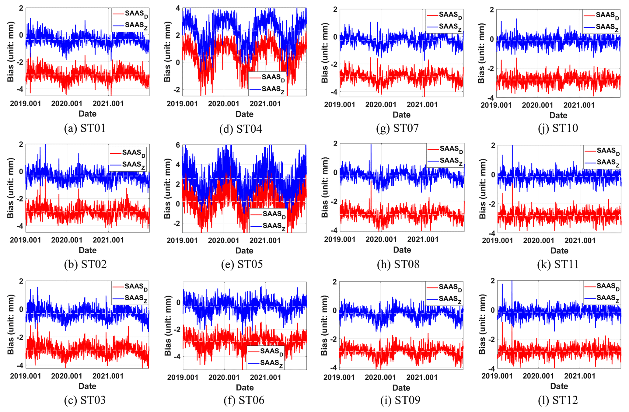
Figure 2Bias time series of the model SAASD and SAASZ. Panels (a)–(l) represent the situations of the 12 sites, respectively. The light-red dotted line and light-blue dotted line show the mean value of bias series from SAASD and SAASZ, respectively.
Table 1Geodetic coordinates of study areas and corresponding climate types.
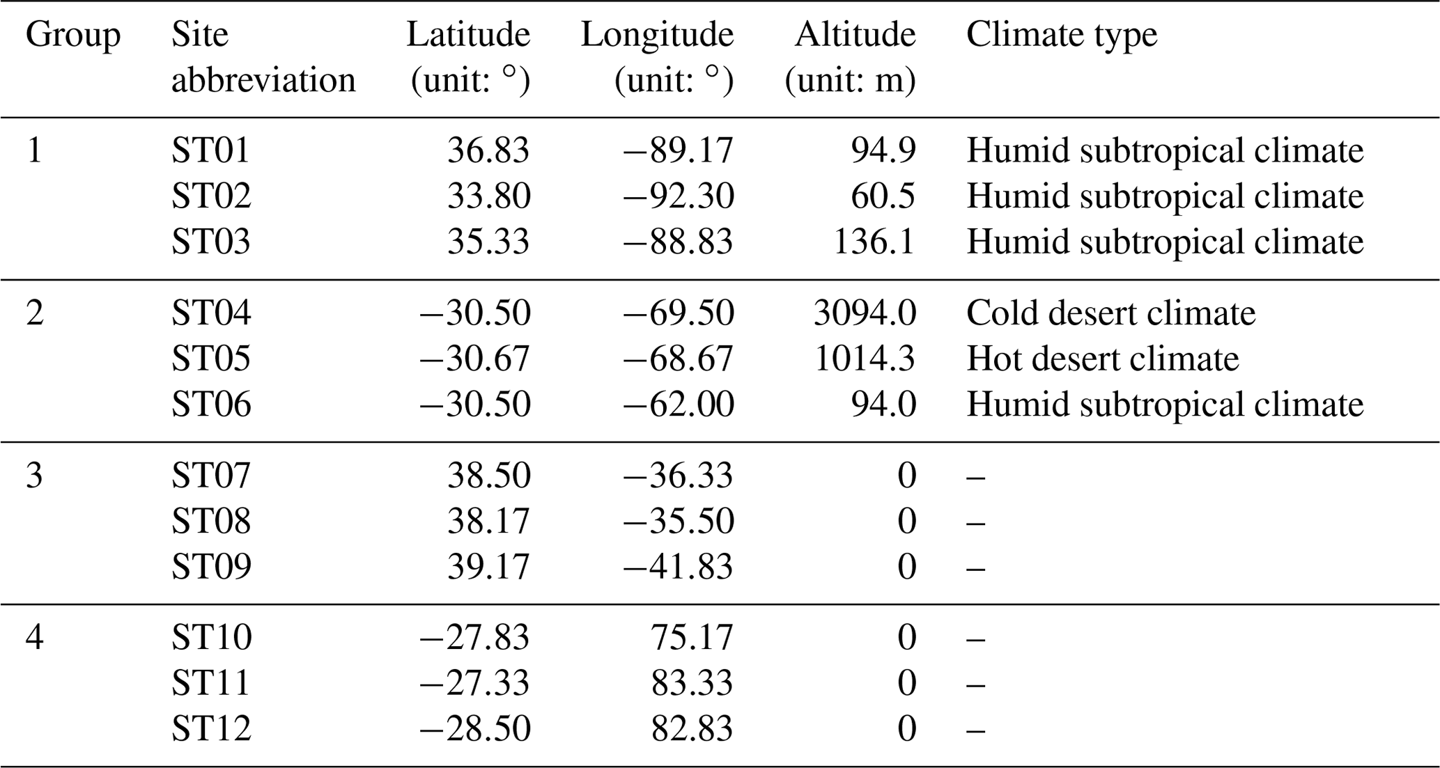
Note: climate type determines the general weather conditions in this area; thus, it probably keeps close relation with ZHD. Because of this, the climate type of each site is displayed here for further analysis, which complies with Köppen–Geiger climate classification. For more details please refer to Peel et al. (2007) and Beck et al. (2018). ST07 to ST12 are located in the middle of the ocean and have no type attribution in the Köppen–Geiger classification, so a “–” was left in the table above.
Table 2Mean absolute bias (MAB)/standard deviation (SD) of SAASD and SAASZ biases (unit: mm).
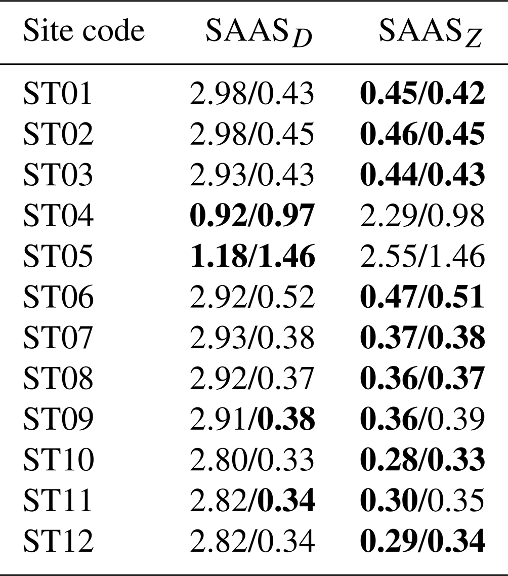
Note: bold numbers represent minimum absolute values in row comparisons.
It can be seen from Fig. 2 that if no correction is applied, the SAASD model would generate about 2.5 mm biases; by contrast, those from SAASZ seem to be restricted to within 0.5 mm mostly (10 sites of 12 in Table 2). Yet, in fact, there exists unknown high-frequency residual information in both ZHD models, and it might be speculated that it should be related to the vertical pressure gradient in each region. Also, it turns out that SAASZ only increases by ∼ 2 mm overall, with the periodic trend still reserved, and the biases' SD of SAASZ keeps almost the same as that of SAASD (Table 2). Besides, from Fig. 2, the SDs in marine areas are generally smaller than those on land, and the value of SD seems to be related to the complexity of climatic condition; for example, the sites in Group 1 show little variety in SDs, while those in Group 2 experience a quite different thing.
Since the difference between the two models is not statistically significant, and SAASD has been used for much longer, we took SAASD for an example in the following part to analyze the characteristics further. The correlation coefficient matrix of biases of 12 sites was shown in Fig. 3, as well as their spectrum analysis diagram (Fig. 4) and proportion of annual and semi-annual periodic terms in the total energy spectrum (Fig. 5).
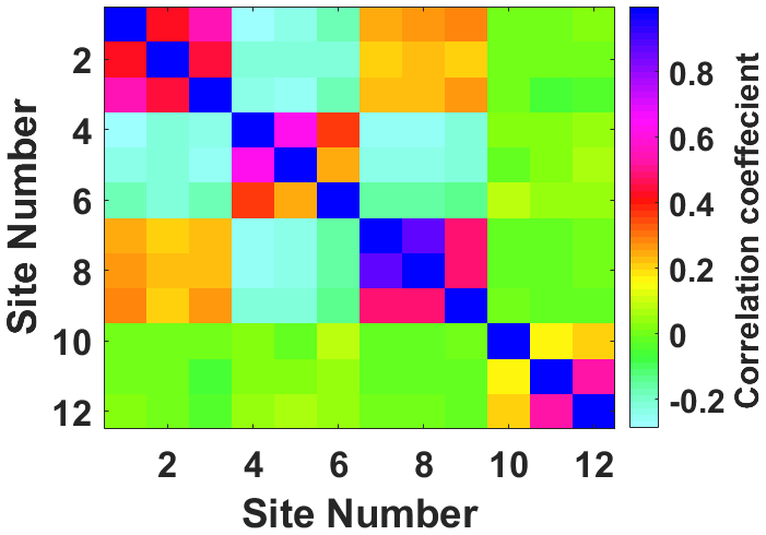
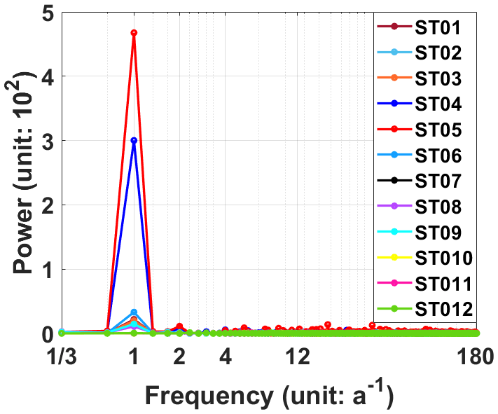
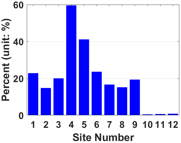
Figure 5Percentage of annual and semi-annual items in total energy for ZHD biases of the model SAASD.
It can be inferred from Fig. 3 that the correlation coefficient becomes larger if the two sites are closer. For instance, the coefficients of the sites within the group are apparently larger than those between groups; also, as ST02 is away from the other two in Group 1, the correlation appears weaker. The same phenomenon can be observed from the relationship between ST06 and the other two in Group 2. When we compare the correlation between Group 1 and Group 2, it can be seen that the correlation is also generally larger in areas with the same climate category or at similar elevation. When it comes to the sites in Group 3 and Group 4, it turns out that the biases in marine areas also vary with the location, and the correlation between them seems stronger than those between the sites with the same distance spacing on land. Combined with the spectrum diagram (Fig. 4), it can be seen that the biases for most sites are generally influenced by annual and semi-annual signals, and the energy intensity varies significantly with the site's location: regions with high altitude appear more sensitive to season, such as ST04 and ST05, while situations for those in the ocean in the Southern Hemisphere are opposite, such as ST10–ST12 (Fig. 5).
3.2 Global analysis
To further analyze the global distribution characteristics of ZHD systematic biases, we calculated the 1 arcdeg grid values of ZHD biases during January–December 2020 and depicted their monthly averaged distributions (Fig. 6) with statistics listed in Table 3. Herein, we have some conclusions.
-
It confirms the seasonal characteristics, which is reflected in varying degrees throughout the world. For instance, the bias values in Northern Hemisphere winter are on average negative, while those in the Southern Hemisphere, especially in high-altitude areas, are positive. Then, with season shifting, the values in the Northern Hemisphere gradually become positive, and those in the Southern Hemisphere winter go the opposite way. This annual regression phenomenon can also be found by combining the MABs and SDs of the global monthly averaged biases in Table 3.
-
Combining with Fig. 1, we find that the biases have a different sign in regions with different altitude. In the Northern Hemisphere in winter, there are more positive values in high-altitude areas (such as the Qinghai Tibet Plateau in Asia and the Andes Mountains in South America), yet more negative ones in marine areas (such as the North Atlantic and the eastern Pacific) or low-altitude land (such as the northwest of the Eurasian continent and northeast of North America). However, this pattern is opposite in Antarctica and areas with high altitude in Greenland. The preliminary judgment may be subjected to the fact that those regions are in the polar high-pressure zone all year round, and the vertical pressure gradient force is usually less than the atmospheric gravity; at this time, the hydrostatic equilibrium is broken, and the closed formula deduced from this condition deviates. Looking back at SAASZ, if this model is used, biases in areas with high altitude will probably become worse.
-
By and large, biases in the Southern Hemisphere (except Antarctica) vary with latitude even in different seasons. Considering that the ocean area in the Southern Hemisphere is much larger than the land, and the meteorological condition is dominated by oceans, whose physical characteristics are affected by solar energy and closely related to latitude, this probably leads to the latitudinal distribution. As a counterexample, that pattern is weak in the Northern Hemisphere.
-
Overall, the MAB of SAASD over the whole year is ∼ 0.77 mm, not that large, but it changes significantly with season and geographical location, and the difference between the maximum and minimum values exceeds 30 mm, especially in the Northern Hemisphere in summer (Table 3). Hence, such kinds of biases should be fully considered in the field of high-precision measurement.
-
Looking back at the SAASZ model, it is only modified in terms of the coefficient of C, which is equivalent to an overall enlargement of ∼ 0.11 % on the basis of the SAASD. Therefore, the SAASZ model will also experience biases similar to the SAASD, yet their variation with geographical location may differ from that of the latter model. For this reason, a correction is necessary for SAASZ as well.
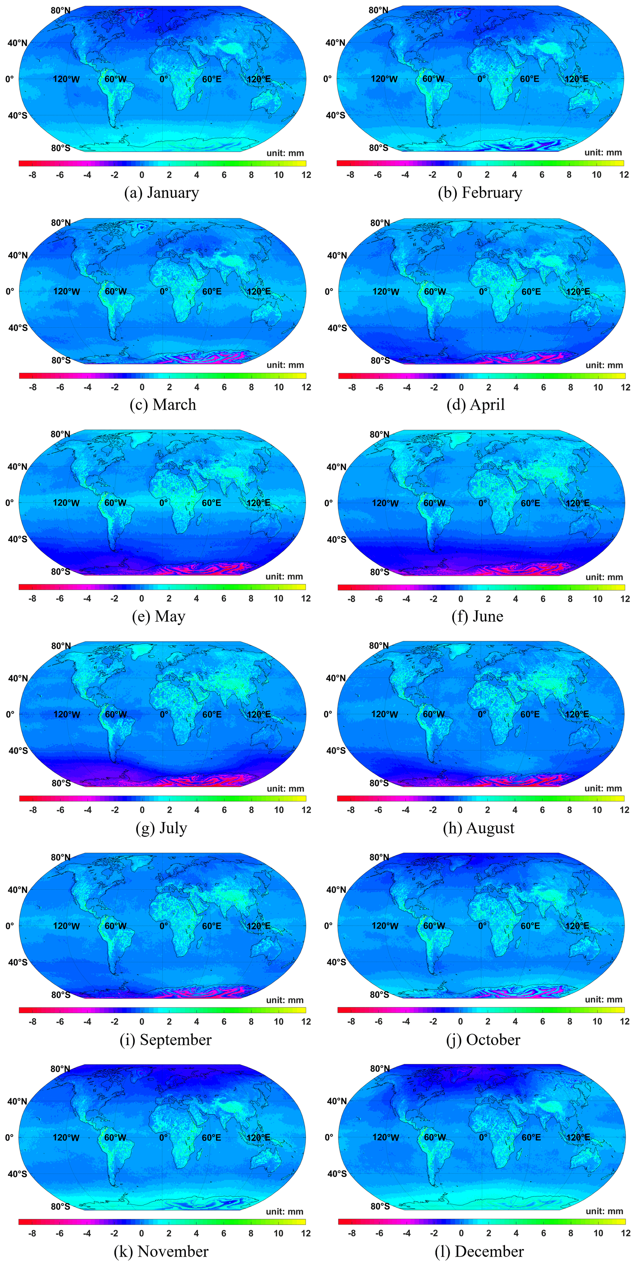
Figure 6Global distribution maps of monthly averaged ZHD systematic biases between SAASD ZHD and integral ZHD. Panels (a)–(l) represent the monthly averaged biases from January to December 2020. In order to distinguish the variations between different months, we use the same scale color bars in the 12 panels above.
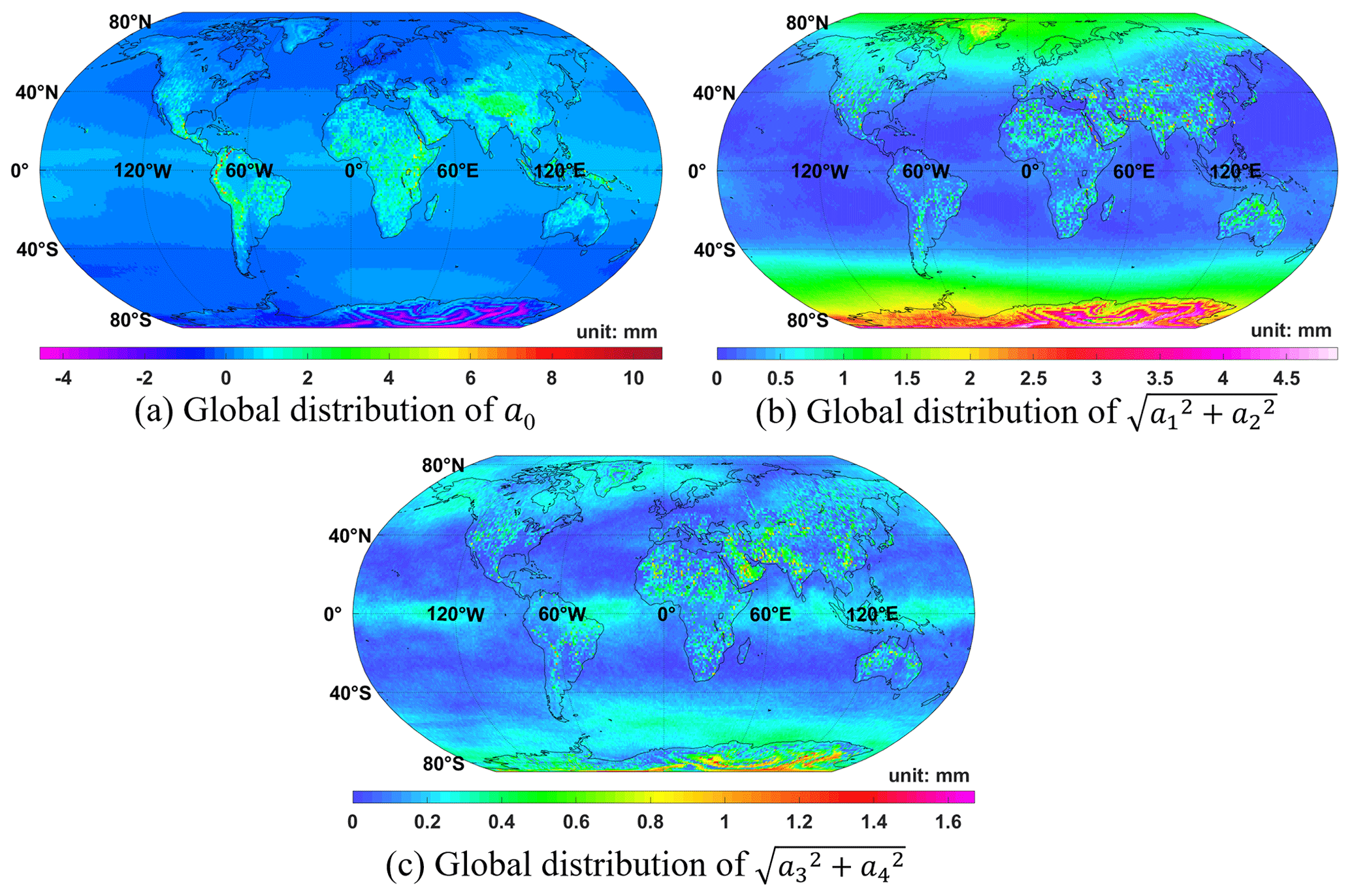
Figure 7Global distribution of coefficients as a periodic function. Changes in the constant term and annual and semi-annual amplitudes are described in (a)–(c), respectively.
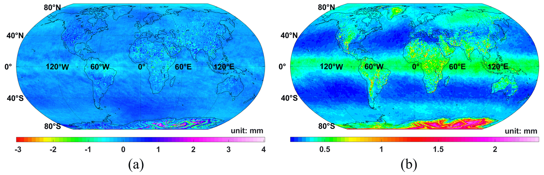
Figure 8MABs over July (a) and the whole year (b) of 2020 after correction by the grid model.
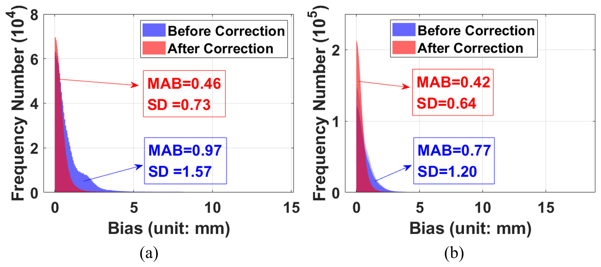
Figure 9Frequency distribution of MABs over July (a) and the whole year (b) of 2020 before and after correction.
Table 3Statistics of systematic biases in different months and the whole year (unit: mm).
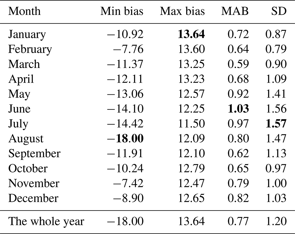
Note: bold numbers represent minimum absolute values in column comparisons.
3.3 Grid correction model
Based on the periodic characteristics that the biases perform in the above experiments, we approximated them using a trigonometric function as Eq. (8), which contains annual and semi-annual periodic terms.
where δZHD is the approximated ZHD bias; a0–a4 represent annual average and annual and semi-annual periodic term coefficients, respectively; and t stands for the day of year (DOY) (Böhm et al., 2015; Landskron and Böhm, 2018). The parameters were estimated using the biases of each grid point on a global scale in 2020, and the distributions of a0, , and are depicted in Fig. 7, where and denote the amplifications of annual and semi-annual periodic terms, respectively. Because of the location-related feature (based on Sect. 3.1), a grid correction model plus space interpolation are applicable to recover the bias at any position at any time during the year 2020. Five model parameters (a0–a4) will be needed for each grid point. Once the δZHD is calculated, it will just serve as the correction of the ZHD model. We call it ZHD_crct.
From Fig. 7 we have the following conclusions:
-
In mid- and low-latitude areas, the annual average of ZHD biases clearly varies with terrain (or air pressure, since pressure generally decreases with increasing height), which is maintained between −0.2–0.4 mm in ocean and plain areas and ranges from 1.0 to 10.0 mm in high-altitude areas like plateaus and mountains. Results seem to be reversed in cold high-latitude areas, such as Greenland (Arctic) and some of Antarctica, for annual average decreases to −4 mm or even lower.
-
The annual amplitudes in the mid- and low-latitude marine areas are significantly smaller than those in high-latitude land areas. Therefore, if we do not ask for high accuracy, the annual variation in these areas can be directly neglected. However, on the land and in high-latitude areas, especially in Antarctica, Greenland, southern and western Asia, northeastern and northwestern Africa, and other regions, this variation should be well considered since the annual impact reaches ±4 mm or more.
-
The amplitudes of the semi-annual periodic term are insignificant, by and large, yet in areas with a strong annual signal, the semi-annual effect is still obvious enough, even reaching ∼ 1.6 mm. In addition, in the ocean areas near the Equator, the semi-annual signal sticks out from its surroundings, which requires further study.
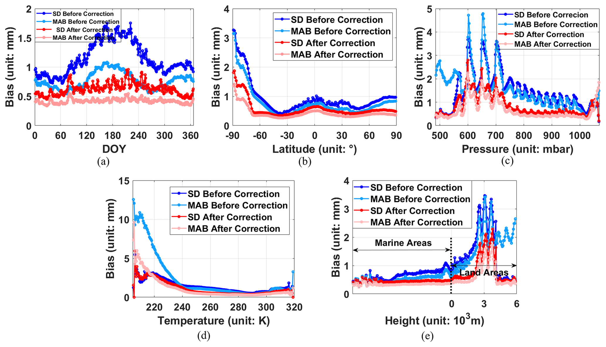
Figure 10The MAB and SD of biases in different dimensions before and after correction over 2020. Panel (a) represents the global MABs and SDs on different DOYs, (b) represents the MABs and SDs at different latitudes, (c) represents the MABs and SDs in regions with different air pressures, (d) represents the MABs and SDs in regions with different temperatures, and (e) represents the MABs and SDs in regions with different heights.
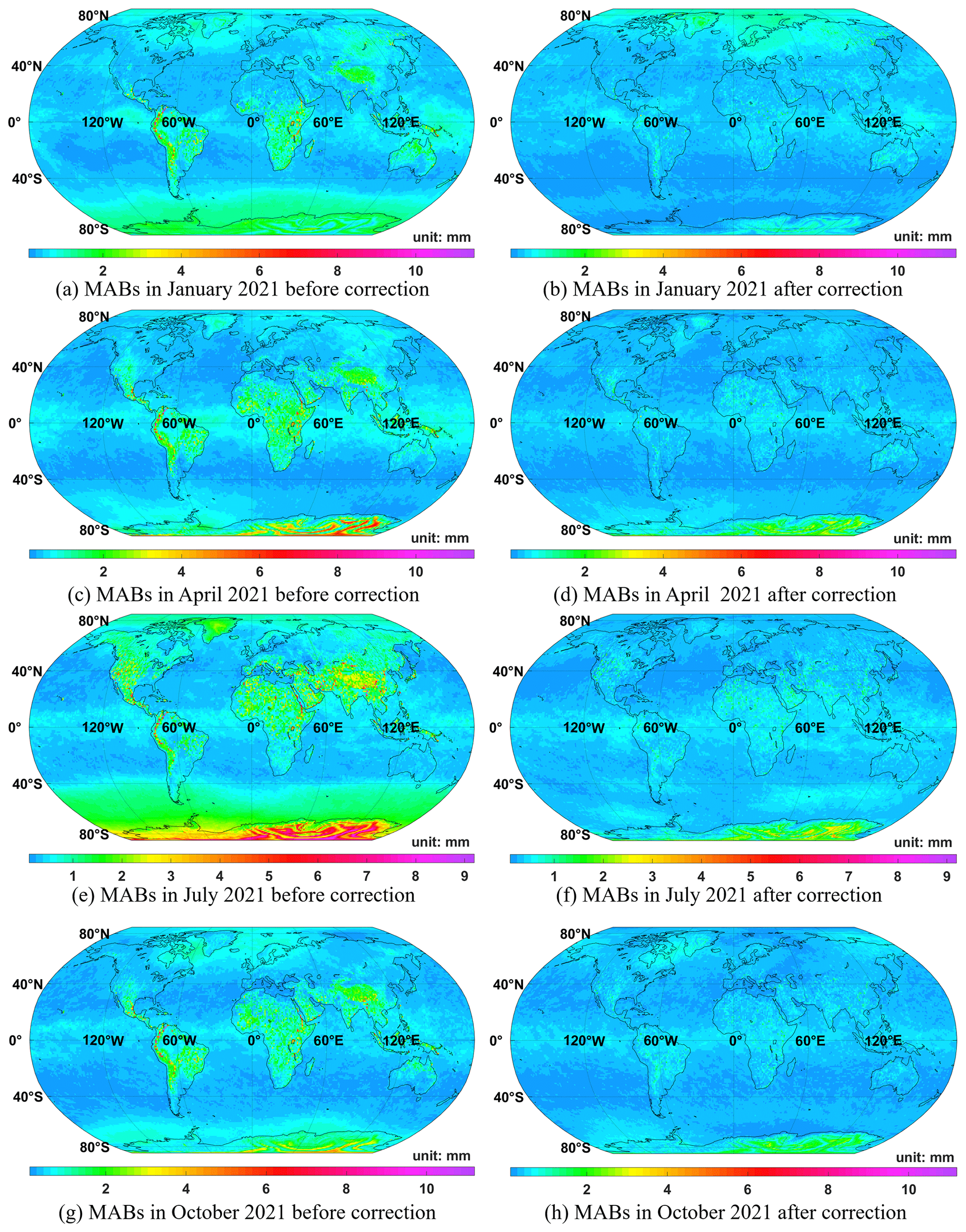
Figure 11Global MABs before (left ones) and after (right ones) correction by the grid model over January (a–b), April (c–d), July (e–f), and October (g–h) in 2021. Please note that the color bar of each month is different.
4.1 Internal coincidence examination
We collected the residual biases of ZHD during 2020 after ZHD_crct being added to check the model's internal coincidence. As the global SD in summer in the Northern Hemisphere reaches the maximum, here the monthly averaged biases of July are depicted for instance in Fig. 8a, as well as the distribution chart of their frequency number before and after correction in Fig. 9a. Also, the annually averaged MABs and their statistical feature can be referred to in Fig. 8b and Fig. 9b. Comparing Fig. 8 and Fig. 6g, it can be seen that the corrected biases are less than ±0.5 mm in most regions of the world, even in mountainous and plateau regions; positive and negative values are nearly evenly distributed in the Northern Hemisphere and Southern Hemisphere, and from Fig. 9, the MABs and SDs are sharply reduced by ∼ 50 % over both July and the whole year. However, biases larger than ±2 mm still exist in Antarctica, the Andes Mountains, and parts of the continents of Asia and Africa, and the improvement near the Equator appears to be not that good compared with other mid- and low-latitude places, similar to the situation of semi-annual amplitudes (Fig. 8b).
Figure 10 shows the MAB and SD of biases in different dimensions before and after correction, in which (a) represents the global MABs and SDs on different DOYs, (b) represents the MABs and SDs at different latitudes, (c) represents the MABs and SDs in regions with different air pressures, (d) represents the MABs and SDs in regions with different temperatures, and (e) represents the MABs and SDs in regions with different heights.
As can be seen from Fig. 10, the corrected biases have been significantly cut down in different dimensions. Figure 10a shows that the annual and semi-annual trends of biases are basically removed. The biases are weakened the most in winter and summer, and the SDs decrease by about 50 % in all periods of the year. Figure 10b shows that the improvement in high-latitude regions and in the Southern Hemisphere at mid-latitudes and low latitudes is superior; by contrast, the reduction in SDs of biases in the Antarctic region was not significant enough compared with that in other regions. Figure 10c shows that the reduction in the low-pressure (600–750 mbar) areas is weaker than that in other areas; these areas are mainly near the south pole, which is basically consistent with the previous conclusion. At the same time, the improvement in the high-pressure (above 1000 mbar) areas is also insignificant, which needs to be further studied. Figure 10d shows that in low-temperature (below 240 K) areas (also mainly near the south pole), the improvement does not stick out from the others; although the MABs are reduced by half, the SDs are not significantly improved compared with those before correction. Figure 10e shows that the improvement is more obvious in land areas with an altitude below 3000 m or over 5000 m.
In terms of the views above, it can be summarized that if no correction is made near the south pole, the error in ZHD by SAASD can be as large as 10 mm or worse; in the Northern Hemisphere in summer, in the regions with pressure lower than 750 mbar, with the temperature lower than 260 K, or most land areas, if no correction is applied, the biases of the ZHD model will be larger than 1 mm generally.
4.2 External coincidence examination
In order to learn the external coincidence of this grid model, we collected the global biases over the year 2021 before and after correction using ZHD_crct, which was fed with coefficients solved according to 2020 bias series. Results of 4 months' MABs are depicted for comparison (Fig. 11), and the statistics of biases (Table 4) and the MAB and SD of biases in different dimensions (Fig. 12) are also exhibited.

Figure 12The MABs and SDs of biases in different dimensions before and after correction over 2021. Panel (a) represents the global MABs and SDs on different DOYs, (b) represents the MABs and SDs at different latitudes, (c) represents the MABs and SDs in regions with different air pressures, (d) represents the MABs and SDs in regions with different temperatures, and (e) represents the MABs and SDs in regions with different heights.
Table 4Statistics of systematic biases before/after correction in different months and the whole year of 2021 (unit: mm).
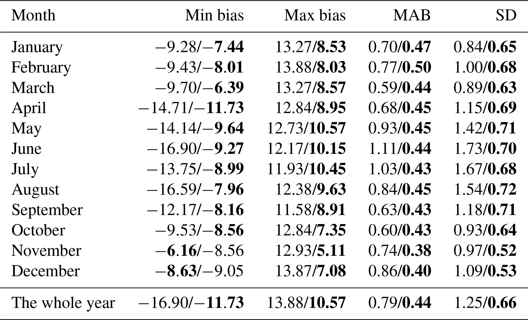
Note: bold numbers represent minimum absolute values in row comparisons.
From the charts above, it is clear that the correction made according to the biases of 2020 still works in 2021, and the improvement over the 2 years seems alike, which means that it is feasible to use historical meteorological data to predict the future bias corrections.
We made a detailed analysis of the biases from the traditional ZHD model. If no correction is applied, SAASD, one of the most widely used models, would generate biases at the millimeter level. Although the MAB over the whole year is ∼ 0.77 mm, biases differ significantly with season and geographical location and reach ±10 mm or even larger, and the difference between the maximum and minimum values exceeds 30 mm. Therefore, it should be fully considered in the field of high-precision measurement, especially for the regions near the south pole and those with pressure less than 750 mbar, temperature less than 260 K, and most land areas.
In order to cut down the biases, a grid model, ZHD_crct, was constructed exploiting a periodic function based on the meteorological data of the current year from ECMWF. Generally, ZHD biases were reduced by ∼ 50 % after correction, with annual and semi-annual terms thoroughly removed, and the model still works when used to rectify the biases in the next year. It can be inferred that this model may be able to forecast corrections in quite a few years. Yet, unfortunately, our model only shows skill in detrending the seasonal impacts, with unknown high-frequency residuals still requiring further study, and this problem is likely to be conquered when we start our study of the vertical velocity of air.
In addition, nowadays profile meteorological parameters can be provided from various organizations, such as MERRA2 data products from the NASA Global Modeling and Assimilation Office, NCEP reanalysis data products, the Integrated Global Radiosonde Archive (IGRA) from the National Climatic Data Center of America (NCDC), and the University of Wyoming Atmospheric Science Radiosonde Archive. Hence, ZHD bias correction models could be further developed based on different datasets in follow-up studies.
The current version of the ZHD_crct model and its corresponding documents are available at https://doi.org/10.6084/m9.figshare.22056884.v1 (Fan et al., 2023). ERA5 data can be obtained from the Copernicus Climate Data Store (https://cds.climate.copernicus.eu/cdsapp#!/dataset/reanalysis-era5-pressure-levels?tab=form, last access: 26 May 2022, https://doi.org/10.24381/cds.bd0915c6, Hersbach et al., 2018). The US Standard Atmosphere 1976 model can be referred to at https://ntrs.nasa.gov/api/citations/19770009539/downloads/19770009539.pdf (Sissenwine et al., 1976). The ETOPO elevation dataset can be downloaded at https://doi.org/10.7289/V5C8276M (Amante and Eakins, 2009).
HF designed the research framework, wrote the paper, and conducted most of the code implementation and data analysis. SL was involved in data collation and revision of the paper. ZS was responsible for supervision. The work in this paper was funded by the programs of GX and XiaL. XinL revised the paper.
The contact author has declared that none of the authors has any competing interests.
Publisher’s note: Copernicus Publications remains neutral with regard to jurisdictional claims in published maps and institutional affiliations.
We thank the Copernicus Climate Change Service (C3S) and Climate Data Store (CDS) for the open data sets, and the helpful work by Norman Sissenwine, Maurice Dubin, and Sidney Teweles is appreciated as well for their efforts in the US Standard Atmosphere 1976. We also thank Christopher Amante and Barry W. Eakins for their elaborate global elevation model ETOPO1.
This research has been supported by the National Natural Science Foundation of China (NSFC) (grant no. 41904039 and grant no. 42174001) and the Young Elite Scientists Sponsorship Program by CAST (2021).
This paper was edited by Thomas Poulet and reviewed by two anonymous referees.
Abdelfatah, M. A., Mousa, A. E., and El-Fiky, G. S.: Precise troposphere delay model for Egypt, as derived from radiosonde data, NRIAG J. Astron. Geophys., 4, 16–24, https://doi.org/10.1016/j.nrjag.2015.01.002, 2015.
Alizadeh, M., Wijaya, D., Hobiger, T., Weber, R., and Schuh, H.: Atmospheric Effects in Space Geodesy, Edition 2013, edited by: Böhm, J. and Schuh, H., Springer, 35–71, ISBN 978-3-642-36931-5, https://doi.org/10.1007/978-3-642-36932-2_2, 2013.
Amante, C. and Eakins, B. W.: ETOPO1 1 Arc-Minute Global Relief Model: Procedures, Data Sources and Analysis, National Geophysical Data Center, NOAA [data set], https://doi.org/10.7289/V5C8276M, 2009.
Beck, H. E., Zimmermann, N. E., McVicar, T. R., Vergopolan, N., Berg, A., and Wood, E. F.: Present and future Köppen-Geiger climate classification maps at 1-km resolution, Sci. Data, 5, 180214, https://doi.org/10.1038/sdata.2018.214, 2018.
Bekaert, D. P. S., Hooper, A., and Wright, T. J.: A spatially variable power law tropospheric correction technique for InSAR data, J. Geophys. Res.-Sol. Ea., 120, 1345–1356, https://doi.org/10.1002/2014JB011558, 2015.
Bevis, M., Businger, S., Chiswell, S., Herring, T. A., Anthes, R. A., Rocken, C., and Ware, R. H.: GPS Meteorology: Mapping Zenith Wet Delays onto Precipitable Water, J. Appl. Meteorol. Climatol., 33, 379–386, https://doi.org/10.1175/1520-0450(1994)033<0379:Gmmzwd>2.0.Co;2, 1994.
Boehm, J., Werl, B., and Schuh, H.: Troposphere mapping functions for GPS and very long baseline interferometry from European Centre for Medium-Range Weather Forecasts operational analysis data, J. Geophys. Res.-Sol. Ea., 111, B02406, https://doi.org/10.1029/2005JB003629, 2006.
Boehm, J., Heinkelmann, R., and Schuh, H.: Short Note: A global model of pressure and temperature for geodetic applications, J. Geod., 81, 679–683, 2007.
Böhm, J., Möller, G., Schindelegger, M., Pain, G., and Weber, R.: Development of an improved empirical model for slant delays in the troposphere (GPT2w), GPS Solutions, 19, 433–441, https://doi.org/10.1007/s10291-014-0403-7, 2015.
Chen, G. and Herring, T. A.: Effects of atmospheric azimuthal asymmetry on the analysis of space geodetic data, J. Geophys. Res.-Sol. Ea., 102, 20489–20502, https://doi.org/10.1029/97JB01739, 1997.
Chen, Z., Zhang, S., and Feng, H.: Research on the correction of troposphere dry delay in GPS positioning and inversing the water vapor in atmosphere, Sci. Meteorol. Sin., 29, 4527–4530, 2009.
Dai, W. and Zhao, Y.: Modeling The Dry And Wet Component Of Regional Tropospheric Delay, J. Geod. Geodyn., 33, 72–76 + 81, https://doi.org/10.14075/j.jgg.2013.02.010, 2013.
Davis, J. L., Herring, T. A., Shapiro, I. I., Rogers, A. E. E., and Elgered, G.: Geodesy by radio interferometry: Effects of atmospheric modeling errors on estimates of baseline length, Radio Sci., 20, 1593–1607, https://doi.org/10.1029/RS020i006p01593, 1985.
Dogan, A. H. and Erdogan, B.: A new empirical troposphere model using ERA5's monthly averaged hourly dataset, J. Atmos. Sol.-Terr. Phys., 232, 105865, https://doi.org/10.1016/j.jastp.2022.105865, 2022.
Drożdżewski, M. and Sośnica, K.: Tropospheric and range biases in Satellite Laser Ranging, J. Geod., 95, 100, https://doi.org/10.1007/s00190-021-01554-0, 2021.
Eriksson, D., MacMillan, D. S., and Gipson, J. M.: Tropospheric delay ray tracing applied in VLBI analysis, J. Geophys. Res.-Sol. Ea., 119, 9156–9170, https://doi.org/10.1002/2014JB011552, 2014.
Fan, H., Sun, Z., Zhang, L., and Liu, X.: A two-step estimation method of troposphere delay with consideration of mapping function errors, Acta Geod. Cartog. Sin., 48, 286–294, 2019.
Fan, H., Li, S., Sun, Z., Xiao, G., Li, X., Liu, X.: Codes and Example data.zip, figshare [data set], https://doi.org/10.6084/m9.figshare.22056884.v1, 2023.
Feng, P., Li, F., Yan, J., Zhang, F., and Barriot, J.-P.: Assessment of the Accuracy of the Saastamoinen Model and VMF1/VMF3 Mapping Functions with Respect to Ray-Tracing from Radiosonde Data in the Framework of GNSS Meteorology, Remote Sens., 12, 3337, https://doi.org/10.3390/rs12203337, 2020.
Graham, R. M., Hudson, S. R., and Maturilli, M.: Improved Performance of ERA5 in Arctic Gateway Relative to Four Global Atmospheric Reanalyses, Geophys. Res. Lett., 46, 6138–6147, https://doi.org/10.1029/2019GL082781, 2019.
Hersbach, H., Bell, B., Berrisford, P., Biavati, G., Horányi, A., Muñoz Sabater, J., Nicolas, J., Peubey, C., Radu, R., Rozum, I., Schepers, D., Simmons, A., Soci, C., Dee, D., and Thépaut, J.-N.: ERA5 hourly data on pressure levels from 1959 to present, Copernicus Climate Change Service (C3S) Climate Data Store (CDS) [data set], https://doi.org/10.24381/cds.bd0915c6, 2018.
Hobiger, T., Ichikawa, R., Takasu, T., Koyama, Y., and Kondo, T.: Ray-traced troposphere slant delays for precise point positioning, Earth, Planets Space, 60, e1–e4, https://doi.org/10.1186/BF03352809, 2008.
Hofmeister, A.: Determination of path delays in the atmosphere for geodetic VLBI by means of ray-tracing, Technische Universität Wien, reposiTUm, 68–69, https://doi.org/0.34726/hss.2016.21899, 2016.
Hofmeister, A. and Böhm, J.: Application of ray-traced tropospheric slant delays to geodetic VLBI analysis, J. Geod., 91, 945–964, https://doi.org/10.1007/s00190-017-1000-7, 2017.
Hopfield, H. S.: Tropospheric Effect on Electromagnetically Measured Range: Prediction from Surface Weather Data, Radio Sci., 6, 357–367, https://doi.org/10.1029/RS006i003p00357, 1971.
Hu, Y. and Yao, Y.: A new method for vertical stratification of zenith tropospheric delay, Adv. Space Res., 63, 2857–2866, https://doi.org/10.1016/j.asr.2018.10.035, 2019.
Landskron, D. and Böhm, J.: VMF3/GPT3: refined discrete and empirical troposphere mapping functions, J. Geod., 92, 349–360, https://doi.org/10.1007/s00190-017-1066-2, 2018.
Leandro, R. F., Langley, R. B., and Santos, M. C.: UNB3m_pack: a neutral atmosphere delay package for radiometric space techniques, GPS Solutions, 12, 65–70, 2008.
Li, W., Yuan, Y., Ou, J., and He, Y.: IGGtrop_SH and IGGtrop_rH: Two Improved Empirical Tropospheric Delay Models Based on Vertical Reduction Functions, IEEE Trans. Geosci. Electron., 56, 5276–5288, https://doi.org/10.1109/TGRS.2018.2812850, 2018.
Li, Y., Zou, X., Tang, W., Deng, C., Cui, J., and Wang, Y.: Regional modeling of tropospheric delay considering vertically and horizontally separation of station for regional augmented PPP, Adv. Space Res., 66, 2338–2348, https://doi.org/10.1016/j.asr.2020.08.003, 2020.
Liu, J., Chen, X., Sun, J., and Liu, Q.: An analysis of GPT2/GPT2w+Saastamoinen models for estimating zenith tropospheric delay over Asian area, Adv. Space Res., 59, 824–832, https://doi.org/10.1016/j.asr.2016.09.019, 2017.
Liu, Y., HBIZ, and Chen, Y.: Precise Determination of Dry Zenith Delay for GPS Meteorology Applications, Acta Geod. Cartog. Sin., 29, 172–180, 2000.
Ma, Y., Liu, T., Chen, P., Zheng, N., Zhang, B., Xu, G., and Lu, Z.: Global tropospheric delay grid modeling based on Anti-Leakage Least-Squares Spectral Analysis and its validation, J. Atmos. Sol.-Terr. Phys., 229, 105829, https://doi.org/10.1016/j.jastp.2022.105829, 2022.
Mendes, V.: Modeling the neutral-atmosphere propagation delay in radiometric space techniques, PhD dissertation, Department of Geodesy and Geomatics Engineering Technical Report No. 199, University of New Brunswick, Fredericton, New Brunswick, Canada, 353 pp., 1999.
Mendes, V. B., Prates, G., Pavlis, E. C., Pavlis, D. E., and Langley, R. B.: Improved mapping functions for atmospheric refraction correction in SLR, Geophys. Res. Lett., 29, 1414, https://doi.org/10.1029/2001GL014394, 2002.
Minzner, R. A.: The 1976 Standard Atmosphere and its relationship to earlier standards, Rev. Geophys., 15, 375–384, 1977.
Nafisi, V., Madzak, M., Böhm, J., Ardalan, A. A., and Schuh, H.: Ray-traced tropospheric delays in VLBI analysis, Radio Sci., 47, RS2020, https://doi.org/10.1029/2011RS004918, 2012.
Niell, A. E.: Global mapping functions for the atmosphere delay at radio wavelengths, J. Geophys. Res.-Sol. Ea., 101, 3227–3246, https://doi.org/10.1029/95JB03048, 1996.
Osah, S., Acheampong, A. A., Fosu, C., and Dadzie, I.: Evaluation of Zenith Tropospheric Delay Derived from Ray-Traced VMF3 Product over the West African Region Using GNSS Observations, Adv. Meteor., 2021, 8836806, https://doi.org/10.1155/2021/8836806, 2021.
Peel, M. C., Finlayson, B. L., and McMahon, T. A.: Updated world map of the Köppen-Geiger climate classification, Hydrol. Earth Syst. Sci., 11, 1633–1644, https://doi.org/10.5194/hess-11-1633-2007, 2007.
Penna, N., Dodson, A., and Chen, W.: Assessment of EGNOS Tropospheric Correction Model, J. Navig., 54, 37–55, 2001.
Rocken, C., Sokolovskiy, S., Johnson, J. M., and Hunt, D.: Improved Mapping of Tropospheric Delays, J. Atmos. Oceanic. Technol., 18, 1205–1213, https://doi.org/10.1175/1520-0426(2001)018<1205:IMOTD>2.0.CO;2, 2001.
Rüeger, J. M.: Refractive Index Formulae for Radio Waves, FIG XXII International Congress, Washington, D.C., 19–26 April, https://www.fig.net/resources/proceedings/fig_proceedings/fig_2002/Js28/JS28_rueger.pdf (last access: 8 February 2023), 2002.
Saastamoinen, J.: Contributions to the theory of atmospheric refraction, Bull. Geod., 105, 279–298, 1972.
Sissenwine, N., Dubin, M., and Teweles, S.: COESA CoChairmen, U.S. Standard Atmosphere, 1976. Stock No. 003-017-00323-0, U.S. Government Printing Office, Washington, D. C. USA [data set], https://ntrs.nasa.gov/api/citations/19770009539/downloads/19770009539.pdf (last access: 8 February 2023), 1976.
Sun, Z., Zhang, B., and Yao, Y.: An ERA5-Based Model for Estimating Tropospheric Delay and Weighted Mean Temperature Over China With Improved Spatiotemporal Resolutions, Earth Space Sci., 6, 1926–1941, https://doi.org/10.1029/2019EA000701, 2019.
Tang, W., Liao, M., Zhang, L., and Zhang, L.: Study on InSAR tropospheric correction using global atmospheric reanalysis products, Chin. J. Geophys., 60, 527–540, 2017.
Thayer, G. D.: A Rapid and Accurate Ray Tracing Algorithm for a Horizontally Stratified Atmosphere, Radio Sci., 2, 249–252, https://doi.org/10.1002/rds196722249, 1967.
Tregoning, P. and Herring, T. A.: Impact of a priori zenith hydrostatic delay errors on GPS estimates of station heights and zenith total delays, Geophys. Res. Lett., 33, L23303, https://doi.org/10.1029/2006GL027706, 2006.
Tuka, A. and El-Mowafy, A.: Performance evaluation of different troposphere delay models and mapping functions, Measurement, 46, 928–937, https://doi.org/10.1016/j.measurement.2012.10.015, 2013.
Wang, J., Balidakis, K., Zus, F., Chang, X., Ge, M., Heinkelmann, R., and Schuh, H.: Improving the Vertical Modeling of Tropospheric Delay, Geophys. Res. Lett., 49, e2021GL096732, https://doi.org/10.1029/2021GL096732, 2022.
Wang, J. J., Wang, J., Sinclair, D., and Lee, H. K.: Tropospheric Delay Estimation for Pseudolite Positioning, Positioning, 1, 106–112, https://doi.org/10.5081/jgps.4.1.106, 2005.
Xiao, R., Yu, C., Li, Z., and He, X.: Statistical assessment metrics for InSAR atmospheric correction: Applications to generic atmospheric correction online service for InSAR (GACOS) in Eastern China, Int. J. Appl. Earth Obs. Geoinf., 96, 102289, https://doi.org/10.1016/j.jag.2020.102289, 2021.
Yan, Y., Wang, J., and Liu, X.: The Model Correction of Dry Zenith Delay of Troposphere Atmosphere in Local Region, GNSS World Chin., 36, 44–46+50, https://doi.org/10.13442/j.gnss.2011.04.007, 2011.
Yao, Y., Guo, J., Zhang, B., and Hu, Y.: A Global Empirical Model of the Conversion Factor Between Zenith Wet Delay and Precipitable Water Vapor, Geomatics Inf. Sci. Wuhan Univ., 41, 45–51, https://doi.org/10.13203/j.whugis20140585, 2016.
Yao, Y., Xu, X., Xu, C., Peng, W., and Wan, Y.: GGOS tropospheric delay forecast product performance evaluation and its application in real-time PPP, J. Atmos. Sol.-Terr. Phys., 175, 1–17, https://doi.org/10.1016/j.jastp.2018.05.002, 2018.
Younes, S. A. M. and Afify, H. A.: Accuracy improvement of tropospheric delay correction models in space geodetic data. Case study: Egypt, Geod. Cartog., 40, 148–155, https://doi.org/10.3846/20296991.2014.987465, 2014.
Zhang, D., Guo, J., Chen, M., Shi, J., and Zhou, L.: Quantitative assessment of meteorological and tropospheric Zenith Hydrostatic Delay models, Adv. Space Res., 58, 1033–1043, https://doi.org/10.1016/j.asr.2016.05.055, 2016.