the Creative Commons Attribution 4.0 License.
the Creative Commons Attribution 4.0 License.
 | 09 Feb 2023
Application of a satellite-retrieved sheltering parameterization (v1.0) for dust event simulation with WRF-Chem v4.1
Sandra L. LeGrand
Theodore W. Letcher
Gregory S. Okin
Nicholas P. Webb
Alex R. Gallagher
Saroj Dhital
Taylor S. Hodgdon
Nancy P. Ziegler
Michelle L. Michaels
Roughness features (e.g., rocks, vegetation, furrows) that shelter or attenuate wind flow over the soil surface can considerably affect the magnitude and spatial distribution of sediment transport in active aeolian environments. Existing dust and sediment transport models often rely on vegetation attributes derived from static land use datasets or remotely sensed greenness indicators to incorporate sheltering effects on simulated particle mobilization. However, these overly simplistic approaches do not represent the three-dimensional nature or spatiotemporal changes of roughness element sheltering. They also ignore the sheltering contribution of non-vegetation roughness features and photosynthetically inactive (i.e., brown) vegetation common to dryland environments. Here, we explore the use of a novel albedo-based sheltering parameterization in a dust transport modeling application of the Weather Research and Forecasting model with Chemistry (WRF-Chem). The albedo method estimates sheltering effects on surface wind friction speeds and dust entrainment from the shadows cast by subgrid-scale roughness elements. For this study, we applied the albedo-derived drag partition to the Air Force Weather Agency (AFWA) dust emission module and conducted a sensitivity study on simulated PM10 concentrations using the Georgia Institute of Technology–Goddard Global Ozone Chemistry Aerosol Radiation and Transport (GOCART) model as implemented in WRF-Chem v4.1. Our analysis focused on a convective dust event case study from 3–4 July 2014 for the southwestern United States desert region discussed by other published works. Previous studies have found that WRF-Chem simulations grossly overestimated the dust transport associated with this event. Our results show that removing the default erodibility map and adding the drag parameterization to the AFWA dust module markedly improved the overall magnitude and spatial pattern of simulated dust conditions for this event. Simulated PM10 values near the leading edge of the storm substantially decreased in magnitude (e.g., maximum PM10 values were reduced from 17 151 to 8539 µg m−3), bringing the simulated results into alignment with the observed PM10 measurements. Furthermore, the addition of the drag partition restricted the erroneous widespread dust emission of the original model configuration. We also show that similar model improvements can be achieved by replacing the wind friction speed parameter in the original dust emission module with globally scaled surface wind speeds, suggesting that a well-tuned constant could be used as a substitute for the albedo-based product for short-duration simulations in which surface roughness is not expected to change and for landscapes wherein roughness is constant over years to months. Though this alternative scaling method requires less processing, knowing how to best tune the model winds a priori could be a considerable challenge. Overall, our results demonstrate how dust transport simulation and forecasting with the AFWA dust module can be improved in vegetated drylands by calculating the dust emission flux with surface wind friction speed from a drag partition treatment.
- Article
(22200 KB) - Full-text XML
-
Supplement
(14706 KB) - BibTeX
- EndNote


Surface roughness features such as rocks, vegetation, and soil ridges created by tillage attenuate wind flow over the soil surface, considerably affecting aeolian sediment transport and dust emission patterns (see reviews by Mayaud and Webb, 2017; Shao et al., 2015). Representing aerodynamic roughness effects and their spatiotemporal dynamics effectively in numerical dust models is therefore critical for estimating and forecasting the spatial patterns, timing, magnitude, and frequency of mineral dust emission accurately (Evans et al., 2016; Fu, 2019; Ito and Kok, 2017; Li et al., 2013; Tegen et al., 2002; Webb et al., 2014a, b). Several methods are available for characterizing vegetation effects in dust emission models (e.g., Evans et al., 2016; Ginoux et al., 2001; Ito and Kok, 2017; Kim et al., 2013; King et al., 2005; Koven and Fung, 2008; Marticorena and Bergametti, 1995; Okin, 2008; Raupach et al., 1993; Tegen et al., 2002). However, many of these techniques require in situ data that are challenging to obtain over large spatial footprints or incorporate parameterizations with dependencies on land use or vegetation datasets that are often out of date or fail to represent the complex three-dimensional heterogeneity of landscape roughness elements (e.g., Pierre et al., 2014; Raupach and Lu, 2004).
Tuning dust models to satellite- and ground-based observations of dust concentrations and dust optical depth has generally been a sufficient approach for making dust models useful for large-scale climate and air quality applications (e.g., Cakmur et al., 2006). These particular applications tend to focus on total atmospheric dust aerosol loading trends instead of individual dust events. If the goal is to capture the general magnitude and frequency of large-scale dust aerosol patterns, tuning practices are often a viable solution to simulated dust emission errors. However, the relatively poor representation of surface roughness effects on wind erosivity in current dust models has limited our capacity to forecast individual dust events accurately in desert regions with vegetation. Furthermore, poor roughness effect representation limits our ability to accurately simulate the influence of land management practices and desertification on spatial and temporal patterns of dust emission (Webb and Pierre, 2018).
Sediment mobilization schemes are often represented in terms of wind friction speed, u*, a scalar parameter commonly used to describe processes related to wind shear stress (τ; note that , and ρ is air density). Near the land surface, u* represents the total wind shear stress (τ) acting on both the horizontal soil surface (τs) and roughness elements (τr) (i.e., ; see Raupach, 1992; Raupach et al., 1993). This process is typically termed drag partitioning and is often expressed in terms of u* rather than τ. Since τ is proportional to u*, we can similarly divide u* into soil surface (us*) and roughness (ur*) components (i.e., ). The wind shear stress that reaches the immediate soil surface (i.e., τs) governs particle mobilization, so dust emission models driven by us* (or wind erosivity) instead of u* may produce better outcomes (e.g., Darmenova et al., 2009; Okin, 2008; Webb et al., 2020). However, this assumption is worth testing for individual modeling applications since more physically sophisticated methods do not always lead to better simulation outcomes, especially when the more advanced modeling approaches are limited by uncertainties in their required input parameters (e.g., LeGrand et al., 2019).
Though roughness elements affecting us* could comprise any ground feature obstructing airflow over the land surface, traditional aeolian transport models generally equate roughness to vegetation cover, with varying degrees of sophistication in their approach. For example, some models restrict or reduce dust fluxes based on static prescribed vegetation or land use attributes (e.g., Ginoux et al., 2001; LeGrand et al., 2019; Woodward, 2001). Others implement dynamic masks or spatially varying dust flux scaling factors based on real-time or climatological datasets derived from greenness fraction, leaf area index, or normalized difference vegetation index satellite data (Asadov and Kerimov, 2019; Collins et al., 2011; Evans et al., 2016; Ito and Kok, 2017; Kim et al., 2013; Kok et al., 2014; Solomos et al., 2019; Spyrou et al., 2022; Tegen et al., 2002; Vukovic et al., 2014). While some of these techniques have proven useful in certain modeling applications, they depend on datasets that primarily highlight plant productivity phases (e.g., Yu et al., 2016), which may not translate well to soil surface sheltering (Okin, 2010).
Chappell and Webb (2016) proposed a method for parameterizing us* in aeolian transport models using remotely sensed surface albedo (ω). Their technique infers the drag partition from shadows (1−ω) cast by roughness elements based on the assumption that shadows can serve as a proxy for the sheltered surface area extent (Chappell et al., 2010). As described in Ziegler et al. (2020), a generalizable form of the Chappell and Webb (2016) approach equates to
where U10 m is the wind speed 10 m a.g.l. (above ground level), and uns* is a normalized us* parameter (unitless) derived from albedo. By using an albedo-based calculation for each pixel area, the Chappell and Webb (2016) method provides an areal estimate of us* for both the sheltered and non-sheltered zones of the soil surface within each grid pixel.
Here, we explore the use of the Chappell and Webb (2016) albedo-based drag partition within the Weather Research and Forecasting model with Chemistry (WRF-Chem). WRF-Chem is a physically based Earth system model that simulates atmospheric motion on a non-hydrostatic, Eulerian grid in addition to the emission, transport, and mixing of gases and aerosols simultaneously with the meteorology (Fast et al., 2006; Grell et al., 2005; Peckham et al., 2017; Skamarock et al., 2019). The WRF-Chem framework is configurable and can be run with a variety of aerosol and atmospheric chemistry parameterizations, depending on a user's specific interests and computational resources. For this effort, we chose to use the AFWA dust emission module (LeGrand et al., 2019) with the Georgia Institute of Technology–Goddard Global Ozone Chemistry Aerosol Radiation and Transport (GOCART) model (Chin et al., 2000; Ginoux et al., 2001) as implemented in WRF-Chem v4.1.
The AFWA dust emission equations assume that wind-driven dust entrainment primarily occurs through a process called saltation bombardment, in which wind-lofted sand-sized particles (∼ 50–2000 µm diameter) too heavy to remain suspended in the air collide with the land surface and eject smaller dust-sized particles (generally <20 µm diameter) upon impact (e.g., Gillette, 1977; Kok et al., 2012). Several studies have investigated the use of the AFWA dust emission module for a variety of dust modeling applications (e.g., Aragnou et al., 2021; Francis et al., 2022; Hamzeh et al., 2021; Karumuri et al., 2022; Kuchera et al., 2021; Mesbahzadeh et al., 2020; Miller et al., 2021; Mohebbi et al., 2019; Péré et al., 2018; Saidou Chaibou et al., 2020; Solomos et al., 2018; Teixeira et al., 2016; Tsarpalis et al., 2018, 2020; Uzan et al., 2016; Xu et al., 2017; Zhang et al., 2022; Zhou et al., 2019). In general, these studies highlight useful applications of the model. However, several authors noted the need for improved dust source and land surface characterizations in regions with heterogeneous terrain (Cremades et al., 2017; Fountoukis et al., 2016; Hyde et al., 2018; Kim et al., 2021; Ma et al., 2019; Mohebbi et al., 2020; Nabavi et al., 2017; Nguyen et al., 2019; Nikfal et al., 2018; Parajuli et al., 2019, 2020; Parajuli and Zender, 2018; Rizza et al., 2016, 2021; Spyrou et al., 2022; Su and Fung, 2015; Yuan et al., 2019; Zhao et al., 2020).
Here, we aim to evaluate the sensitivity of dust transport simulated by WRF-Chem to the Chappell and Webb (2016) albedo-based drag partition. Our analysis focused on a convective dust event case study from 3–4 July 2014 for the southwestern US desert region previously discussed in other published works (e.g., Hyde et al., 2018; Yu and Yang, 2016). The results from Hyde et al. (2018), in particular, motivated our case study choice. They found that the AFWA dust emission scheme used in WRF-Chem grossly overestimated dust transport for this event. We hypothesized that better geographic sheltering-effect representation from the Chappell and Webb (2016) drag partition would improve the overall magnitude and spatial pattern of the emitted dust and ultimately result in an improved simulation of transported dust. This hypothesis is further strengthened by recent findings from Bukowski and van den Heever (2022), who found that accurate roughness effect characterizations are critical for predicting dust patterns associated with cold pool events similar to our chosen case study.
2.1 Dust emission flux calculation
The AFWA dust emission module (LeGrand et al., 2019) is an adaptation of the dust emission scheme originally described by Marticorena and Bergametti (1995). Equations comprising the AFWA code are in terms of u* and primarily include the threshold friction speed required for particle entrainment over an idealized smooth surface (u*ts), the horizontal saltation flux (Q), the bulk vertical dust flux (FB), and the size-resolved emitted dust flux. For a detailed overview of the dust emission module equations, see LeGrand et al. (2019). The following two subsections summarize the main components of the AFWA dust emission model and the modifications required to incorporate the Chappell and Webb (2016) drag partition.
2.1.1 The original AFWA module configuration
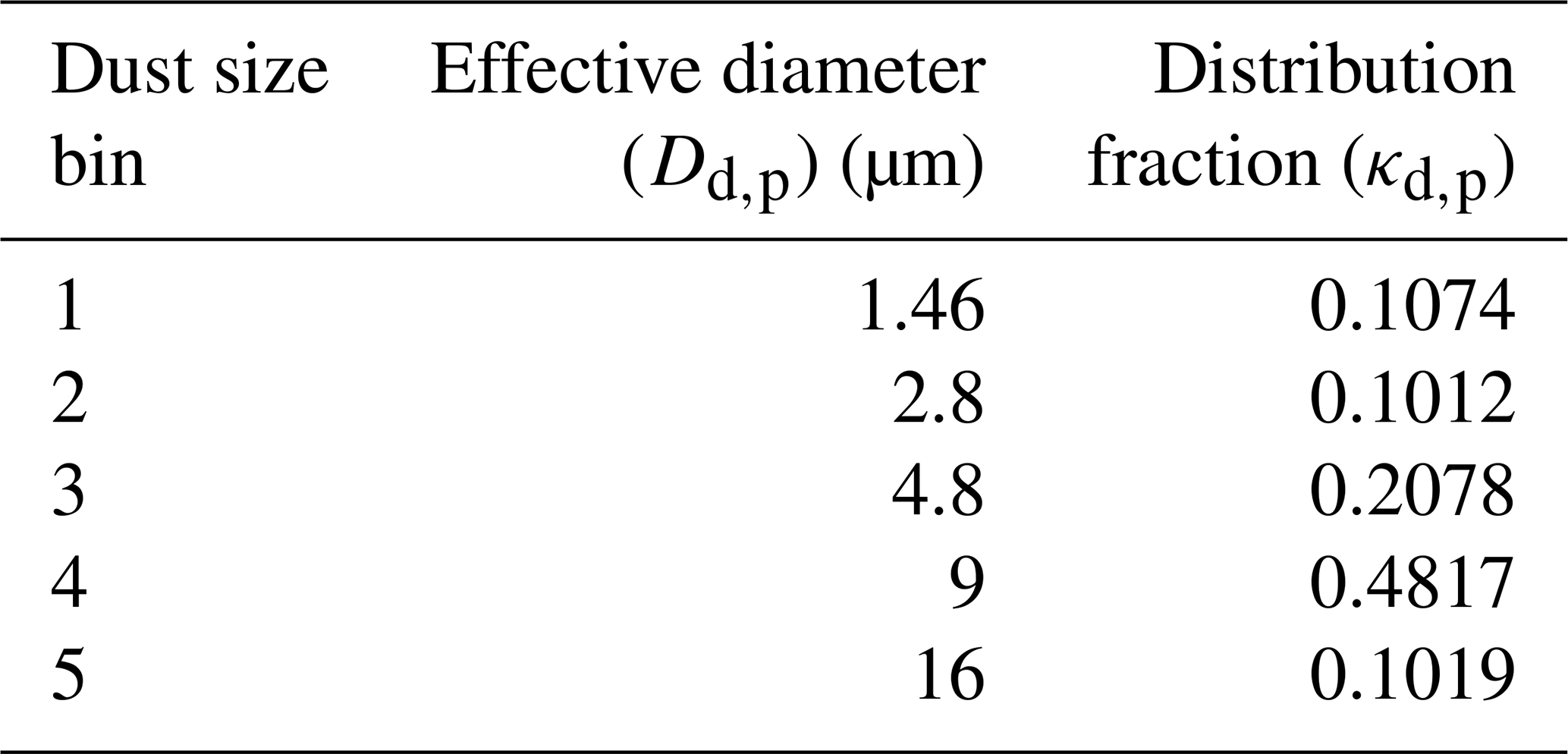
In the AFWA dust emission calculation, soil particles are divided into a predetermined number of bins based on their effective particle size (referred to as size bins). Tables 1–2 provide attributes associated with the nine size bins used for saltation-based processes and the five size bins used for emitted dust. Here, we denote effective diameters for saltation and dust particles by Ds,p and Dd,p, respectively.
Table 1Saltation particle size bins and their associated effective diameters (adapted from LeGrand et al., 2019, Table 1). Particle diameters are presented here in micrometers but handled in units of centimeters within the model.
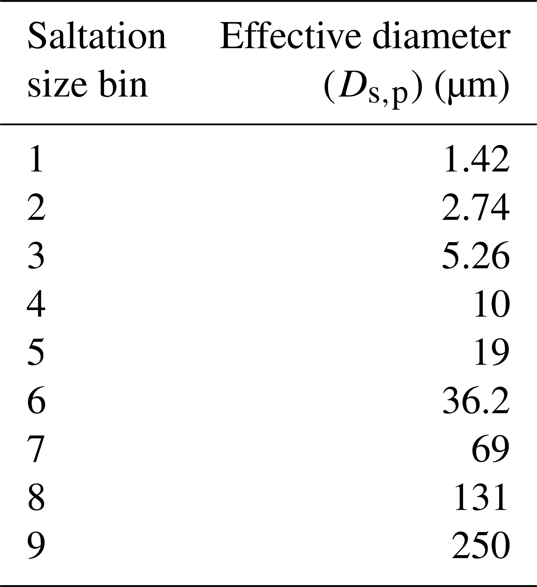
Table 2Dust particle size bins and their associated attributes (adapted from LeGrand et al., 2019, Table 2). Particle diameters are presented here in micrometers but handled in units of centimeters within the model.
As the simulation evolves, saltation for a given size bin initiates and ceases as u* exceeds or falls below size-resolved values of u*ts, respectively. First, the module generates a semi-empirical u*ts estimate (in units of centimeters per second) for each saltation size bin, , assuming air-dry soil conditions:
where g=981 cm s−2 is the gravitational constant, ρa is the spatiotemporally varying air density from the lowest model atmospheric layer, ρs,p is the particle density of saltation bin p, x=1.56, amb=1331 cm−x, and bmb=0.38. The code then applies a correction function, f(θ), that incorporates soil water content and clay composition to account for the effects of soil moisture on particle cohesion based on the approach of Fécan et al. (1999):
Next, the module diagnoses size-resolved saltation flux (Q(Ds,p): in units of grams per centimeter per second) values for each saltation size bin following
where C is an empirical proportionality constant set to 1.0. The module then multiplies Q(Ds,p) by bin-specific weighting factors (dSrel) determined from prescribed mass distribution assumptions and spatially varying sand, silt, and clay mass fractions. The integrated sum of the weighted Q(Ds,p) values determines the total streamwise saltation flux, Q, associated with each model grid cell:
After determining Q, the module generates the bulk vertical dust emission flux (FB; in units of grams per centimeter squared per second) triggered by saltation by multiplying the Q field by a topographic-based dust source strength parameter (S) and a sandblasting efficiency factor (β; in units of value per centimeter) derived from the soil clay fraction. The FB calculation also includes an aerodynamic roughness length (z0) conditional to limit dust emission to non-urban regions with relatively sparse vegetation coverage:
where
and mclay is the soil clay mass fraction. Here, z0 represents the theoretical height at which the mean wind speed near the surface falls to zero due to surface-induced drag (e.g., Stull, 1988; Zobeck et al., 2003). Importantly, this z0 parameter is not part of the new drag partition treatment, but rather a value from the parent WRF model used for a variety of land surface and airflow processes and diagnostics.
Effectively, the mclay conditional in Eq. (7) limits the sandblasting efficiency parameter to 1.06 × 10⁻⁶ cm−1 when the soil composition exceeds 20 % clay content. However, as noted by LeGrand et al. (2019), the β function primarily serves as a dimensional scaling factor. The overall effects of soil clay content variability on FB are relatively small.
The S parameter (originally described by Ginoux et al., 2001) represents the availability of loose erodible soil material at a given location based on the degree of topographic relief of the surrounding area. This approach assumes that soil composition remains consistent over time, and the simulated land surface will neither run out of dust material nor acquire new dust material through fluvial or atmospheric deposition as the simulation evolves. Some papers refer to this spatially varying S field as an erodibility or dust source map. However, both labels provide an inaccurate description of how S functions in the AFWA module. Accordingly, we will not use that terminology here. Essentially, S is a spatially varying tuning parameter ranging from 0 to 1 that assumes that erodible material accumulates in low points in the terrain, determined by
where zi is the elevation of the cell, and zmax and zmin are the maximum and minimum terrain elevation in the surrounding 10∘ × 10∘ area, respectively.
Of note is that the AFWA module uses interpolated values of S initially derived from a elevation dataset. In addition, the S field incorporates a static vegetation mask that blocks dust emission (i.e., S=0) from vegetated areas derived from a 1∘ × 1∘ resolution land cover dataset. While these settings may be appropriate for some modeling applications, the coarse nature of these input datasets likely limits the spatial viability of S at mesoscale and convective-permitting model resolutions (e.g., Saleeby et al., 2019; Vukovic et al., 2014; Walker et al., 2009).
Next, the module applies a prescribed particle size distribution derived using the Kok (2011) brittle fragmentation theory to obtain size-resolved dust emission fluxes:
where F(Dd,p) is the size-resolved emitted dust flux (in units of grams per centimeter squared per second) and κd,p is the distribution fraction of the suspended dust size bin (see Table 2). Lastly, the AFWA module uses F(Dd,p) values to determine the size-resolved dust concentrations injected into the first model atmospheric level for transport during each model time step. From this point forward, functions from other modules in the GOCART suite take over processing the fate and transport of the airborne dust aerosols.
2.1.2 Incorporation of drag partitioning
To obtain gridded values of uns* for use in WRF-Chem, we estimated surface shadowing using data from the snow-masked 500 m Moderate bidirectional reflectance distribution function (BRDF) albedo daily product (Hall and Riggs, 2016; Schaaf and Wang, 2021a). Following Chappell and Webb (2016) and Ziegler et al. (2020), we derived the normalized proportion of shadow (represented using a normalized albedo, ωn) by
where ωdir(0∘) is the daily nadir “black-sky” albedo for MODIS band 1 (620–670 nm wavelength; Schaaf and Wang, 2021b) and fiso is the band 1 BRDF isotropic weighting parameter. In essence, Eq. (10) integrates the albedo across viewing angles for a single illumination angle (solar noon), producing an areal shadow estimate that, in theory, represents non-erodible roughness element conditions for an integrated (500 m pixel) area (e.g., Fig. 1 from Ziegler et al., 2020). We then determined daily uns* by
where ωns represents an empirically scaled proportion of shadow obtained via
using the scaling factors a=0.0001 and b=0.1 to align ωns with the ray casting performed on the reconstructed roughness element configurations in the wind tunnel study by Marshall (1971).

Figure 1A summary overview of the atmospheric forcing conditions associated with a convective dust storm that occurred 3–4 July 2014. The event was characterized by persistent broad high pressure (blue H), clockwise upper-air circulation (black streamlines and arrows), mid- to low-level moisture transport (blue arrows) from the Gulf of California and the Gulf of Mexico, and surface wind vectors (purple arrows) converging downslope of the Mogollon Rim. These conditions initiated and sustained several convective systems that merged near and around Phoenix, Arizona (denoted with a black ×). The shaded overlay shows the national radar reflectivity composite imagery at the storm's peak intensity on 4 July 2014 at 01:00 UTC. Shortly after, the gust front at the leading edge of the convective cell south of Phoenix (dashed black line) moved northwest (storm motion denoted by thin black arrows) over the greater Phoenix area. A wall of thick dust associated with the storm lofted and transported along the gust front.
To incorporate us* into the AFWA dust emission module, we configured WRF-Chem to ingest daily MODIS-derived uns* fields (Eq. 11) that had been interpolated to the model grid domain into the WRF-Chem framework through an auxiliary channel at model runtime and modified the dust emission equations to use us* in place of u*. We then converted daily uns* values to instantaneous us* estimates following Eq. (1) using the WRF-Chem simulated wind speed at 10 m a.g.l. that updates each model time step as U10 m. Finally, we replaced u* in the saltation function from Eq. (4) with us*:
Note that estimated dust emissions are particularly sensitive to small changes in wind friction speed due to the cubed component of the saltation equation (e.g., Tegen et al., 2002). This replacement of u* with us* in Eq. (13) makes the saltation equation consistent with the physics of aeolian transport in the presence of roughness, where excess wind friction speed at the soil surface (i.e., friction speed above the threshold required for particle mobilization) governs the saltation mass flux (Webb et al., 2020). In addition, we added model runtime configuration options to disable the z0 conditional and remove the S factor from the FB function (Eq. 6) since both of these features incorporate broad-scale vegetation masks. Readers are encouraged to review the report by Michaels et al. (2022) for a detailed overview of the code implementation process and model runtime instructions.
The use of the snow-masked version of the MODIS product is essential for this particular modeling application. Although the AFWA module restricts dust emissions from snow-covered areas, the snow-covered grid spaces in the model may not align with snow-covered pixels in the MODIS product. Accordingly, our model implementation process assumes m s−1 for grid spaces with missing data in the MODIS product. This assumption effectively blocks dust emissions from MODIS-detected snow-covered regions and water bodies. We note the potential for missing data problems if the MODIS retrievals have poor spatial coverage. If this scenario occurs, we recommend that users consider filling the gaps through interpolation techniques (assuming the missing data gaps are minimal), using seasonal or monthly climatological uns* values, or using a uns* input dataset from a previous period.
2.2 Description of case study event
As described in detail by Gallagher et al. (2022), our case study dust event was driven by a convective outflow boundary associated with a thunderstorm cluster that developed and evolved over central and southern Arizona following convective weather patterns characteristic of the North American monsoon's summer phase (e.g., Adams and Comrie, 1997). The event began at 18:00 UTC on 3 July 2014, peaked at around 00:00 UTC on 4 July 2014, and concluded mainly by 12:00 UTC on 4 July 2014. At the peak of the event, convective cells organized into an extensive north–south line, pivoting clockwise about its northern end. By 4 July 2014 at 02:00 UTC, the convective line collapsed into three components, with each portion progressing in different directions as they diverged. The gust front associated with the central cell just south of Phoenix, Arizona, generated a thick wall of dust that preceded the storm as it continued west-northwest over the metropolitan area. Figure 1 provides a conceptual overview of the general environmental forcing conditions associated with the dust event. For a more in-depth review of the storm evolution, including synoptic, mesoscale, and local condition assessments using a broad collection of analysis fields, radar composites, and observations for support, we encourage readers to review the Gallagher et al. (2022) report.
Our simulation analysis primarily focused on dust produced by the cell that affected Phoenix. However, we also chose this particular case study because dust concentrations outside the immediate Phoenix area were relatively low in magnitude or negligible. The model's ability to simulate minimal dust loading and dust-free (i.e., clear sky) conditions accurately is also important for it to be a reliable prediction tool. For the simulated results to be considered successful for this case study, the model should be able to both capture the progression of the dust wall over Phoenix and limit dust production from the rest of the broader model domain.
2.3 Model configuration
WRF-Chem is a version of the Weather Research and Forecasting (WRF) model by Skamarock et al. (2019) with additional modules for atmospheric chemistry processes and feedbacks (Fast et al., 2006; Grell et al., 2005). Like WRF, WRF-Chem is a fully compressible finite-difference model that simulates atmospheric motion on the Arakawa C-grid and incorporates a variety of parameterizations for simulating subgrid atmospheric motion, cloud microphysics, radiation, and terrain processes. We used WRF-Chem v4.1 for our test case simulation with WRF parent model configuration settings suggested by Gallagher et al. (2022) and chemistry settings from LeGrand et al. (2019) and Letcher and LeGrand (2018). The study by Gallagher et al. investigated the sensitivity of WRF-simulated atmospheric forcing conditions for the dust event studied here. In particular, they focused on the effects of model initialization (spin-up) time, initial atmospheric conditions, horizontal and vertical model resolutions, and several WRF physics package settings to determine the optimal model configuration that minimized environmental forcing condition errors in the dust simulation.
Table 3 provides a brief overview of the model chemistry and physics configuration. However, complete pre-processor and runtime configuration files (referred to as the namelist.wps and namelist.input files, respectively) for this effort are available from the code repository by Letcher et al. (2022) and in the report by Michaels et al. (2022). The model vertical grid used the default spacing distribution with 40 levels following a stretched hybrid sigma–pressure vertical coordinate that favors higher resolution near the ground. We note that the text and Table 2 from Gallagher et al. (2022) erroneously list their model configuration as having 42 vertical levels instead of 40. However, we confirmed that their study simulations were generated with the same vertical level configuration used for our assessment. Figure 2 displays the three telescoping model domains (D01, D02, and D03, hereafter) with grid resolutions of 18, 6, and 2 km, respectively. In Figs. 3–4, we show key terrain attributes associated with the AFWA dust emission functions for D02 and D03, which primarily encompass the southwestern US desert region.
(Han and Pan, 2011)(Ek et al., 2003)(Nakanishi and Niino, 2004)(Nakanishi and Niino, 2004)(Iacono et al., 2008)(Thompson et al., 2008)(LeGrand et al., 2019)Table 3WRF-Chem physics and chemistry parameterizations. Note that the option numbers may be different in later model versions.
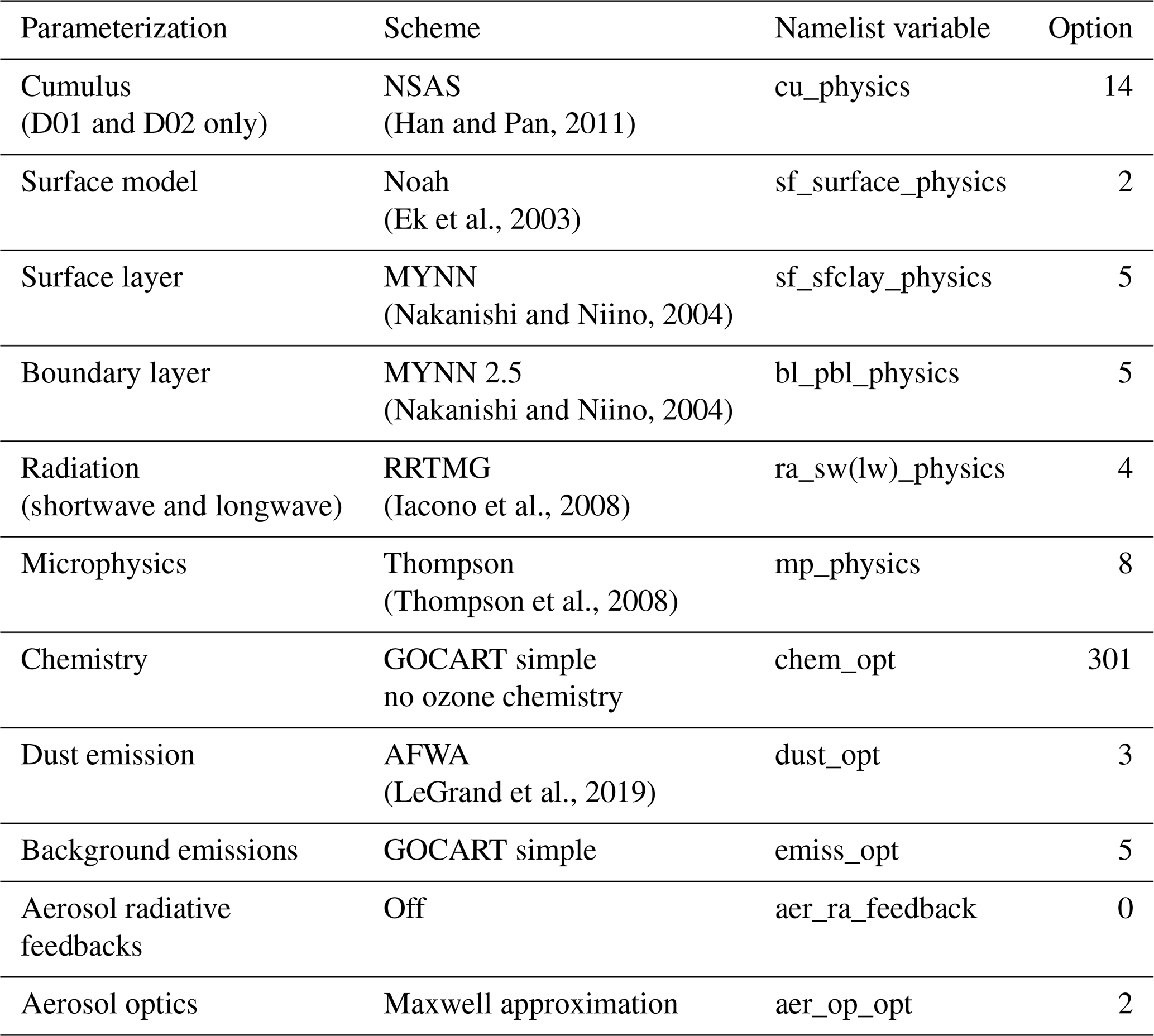
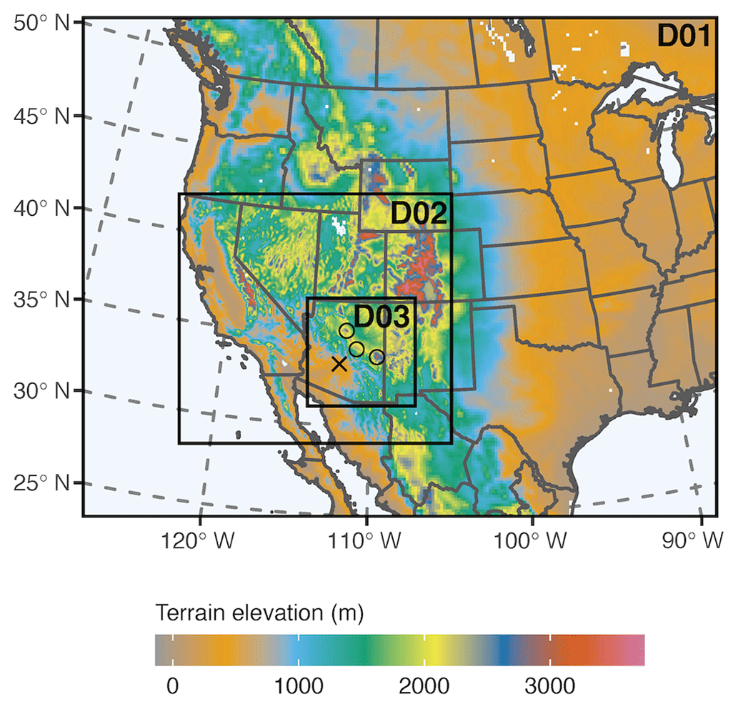
Figure 2Telescoping model domains with shading showing terrain elevation in meters. The black × marks the location of Phoenix, Arizona. The elevated terrain feature northeast of Phoenix marked by a line of hollow circles is the Mogollon Rim.

Figure 3Prescribed land use categories assumed for the model domain. The black × marks the location of Phoenix, Arizona.
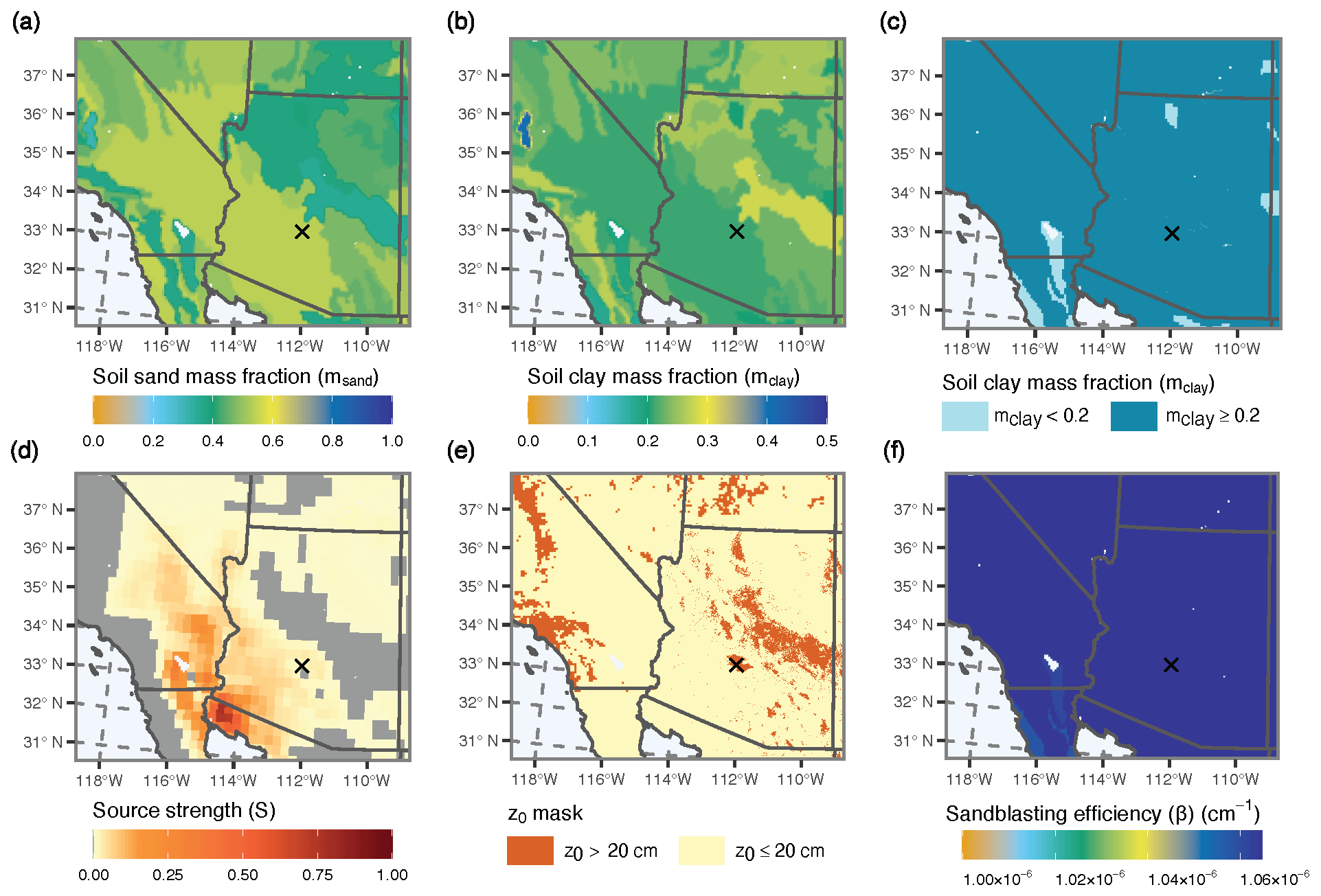
Figure 4Important terrain attribute features considered in the AFWA dust emission flux calculation, including (a) soil sand mass fraction, (b) soil clay mass fraction (mclay), (c) the clay mass fraction threshold affecting dust emission, (d) dust source strength (S; gray areas are masked), (e) the threshold aerodynamic roughness length (z0) required for dust emission, and (f) sandblasting efficiency (β). Note that β (panel f) is relatively homogenous due to the clay-rich soil content of the domain and is capped at 1.06 × 10⁻⁶ cm−1, where the soil composition exceeds 20 % clay content. The black × marks the location of Phoenix, Arizona.
We set the WRF-Chem initial and lateral boundary forcing conditions using 3-hourly analysis fields from the Rapid Refresh Model (Benjamin et al., 2016) supplemented with 6-hourly soil moisture information from the National Centers for Environmental Prediction North American Model analysis product. Though these data are obtainable from multiple resources, we acquired all of our forcing datasets from the National Centers for Environmental Information data portal: https://www.ncei.noaa.gov/products/weather-climate-models/numerical-weather-prediction (last access: 2 February 2023).
We performed our simulations for a 2 d period from 3 July 2014 at 00:00 UTC to 5 July 2014 at 00:00 UTC (2 July 2014 at 17:00 LT to 4 July 2014 at 17:00 LT for Arizona). The first 12 h of the simulation (00:00–12:00 UTC on 3 July 2014) were disregarded as spin-up to allow the model to adjust to the initial and lateral boundary conditions. Atmospheric dust was initialized using a “cold start” approach, which assumes an initial atmospheric dust concentration of zero. Settings engaged by the GOCART simple option in WRF-Chem generated atmospheric fields for other non-dust aerosols, including sea salt, black carbon, organic carbon, and dimethyl sulfide. This particular configuration assumes background sea salt emissions based on the lowest model level wind speeds over the oceans (Gong, 2003) and emissions for the other three aerosol species using climatological emission datasets and the WRF-Chem PREP-CHEM-SRC preprocessing software (Freitas et al., 2011). All dust aerosols originated from the local model domain, meaning that no additional dust aerosols entered the D01 lateral boundaries as the simulations evolved. We consider this a reasonable assumption given the relatively short duration of the case study and because the dust event was generated from localized, convection-induced conditions well within the D01 boundaries.
To better understand the sensitivity of the model to the drag partition treatment, we assessed five test configurations, including a simulation produced using the original AFWA code configuration without a drag partition as a control (CTRL) and four alternative versions using the modified size-resolved saltation treatment from Eq. (13) (see Table 4). The first alternative configuration (ALT1) applied the us*-based Q(Ds,p) estimates and the original FB calculation (Eq. 6), which restricts dust emission from grid cells classified by the model as areas with z0 greater than 20 cm. Because we used the model default 21-class MODIS International Geosphere–Biosphere Programme (IGBP) dataset to characterize land use, this conditional effectively limits dust production to areas classified by the model as barren, grassland, shrubland, savanna, or cropland. The second alternative configuration (ALT2) is identical to ALT1 but with the z0 conditional removed. Our third alternative configuration (ALT3) further simplifies ALT2 by removing the preferential source strength term from the FB calculation (i.e., S=1). Lastly, the fourth alternative configuration (ALT4) estimates us* by applying a global scaling factor (Cs) to U10 m:
with Cs set to a value within the general range of uns* values estimated for the model domain by Eq. (11). Similar to ALT3, the ALT4 configuration also ignores the z0 conditional and assumes S=1.
Table 4Size-resolved saltation and bulk vertical dust flux treatments associated with each test case.
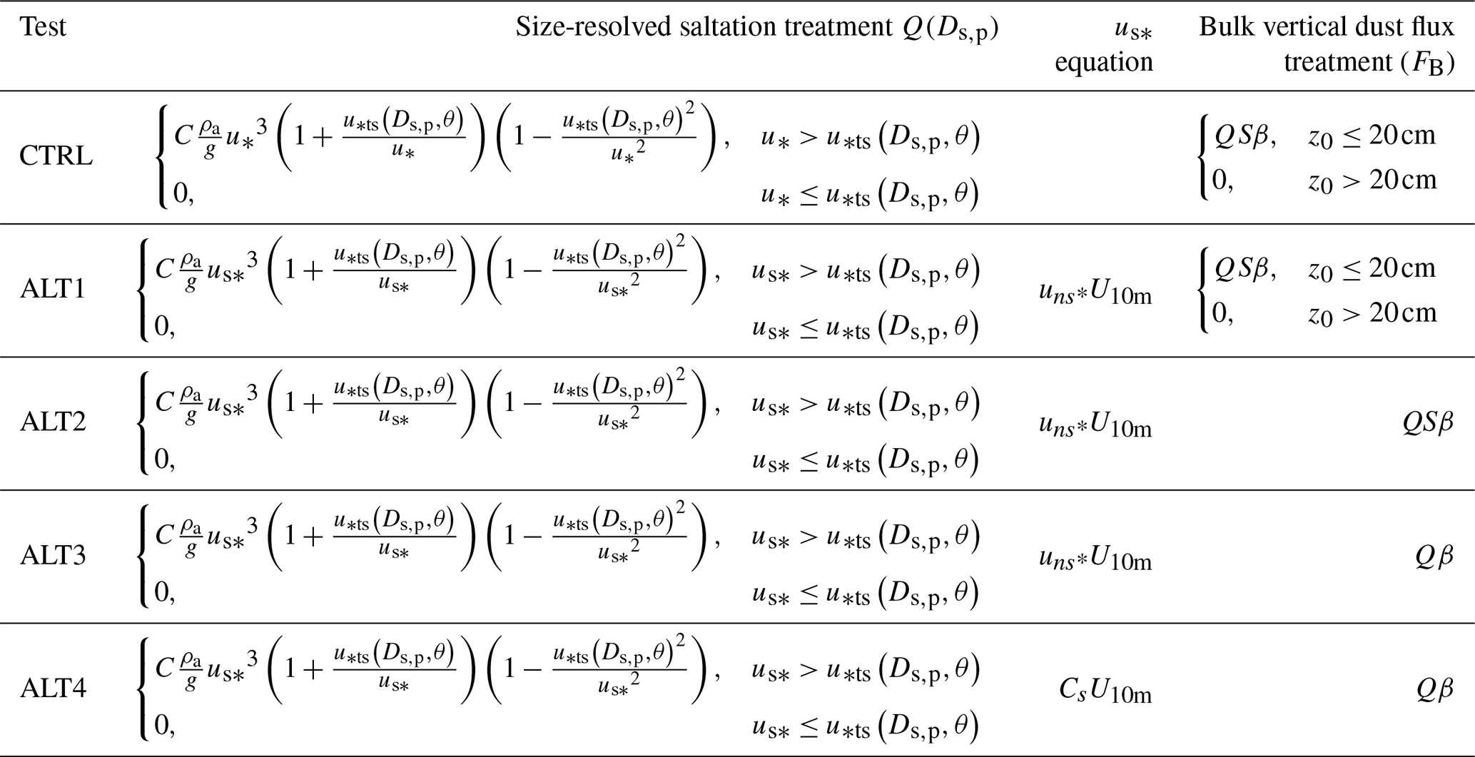
The ALT3 configuration tested the ability of the albedo-based approach to accurately represent the spatially varying surface aerodynamic sheltering afforded by non-erodible roughness elements on the land surface. However, we specifically included the ALT4 configuration to test if the model is able to achieve similar results for this case study event by using globally scaled surface winds without the additional input data acquisition and preprocessing requirements inherent to the Chappell and Webb (2016) method. In other words, ALT4 explores if a model user could achieve the same outcome as the Chappell and Webb (2016) drag partition scheme by simply tuning down the winds if the dust source areas in their domain of interest were generally prone to coverage by vegetation or other roughness elements. Effectively, ALT3 and ALT4 are the only model configurations without some form of vegetation mask built into the dust emission code (see Fig. 5).
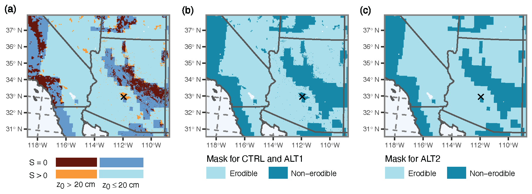
Figure 5Erodible and non-erodible areas associated with the prescribed roughness and S parameter masks. Erodible area masks in the plot on the left (a) largely overlap; maroon indicates regions masked by both the z0 conditional and S parameter, the darker blue represents the area masked by only the S parameter, and orange implies the masking is isolated to the z0 conditional. Light blue regions in (a) have no masking. The middle panel (b) shows the combined z0 and S parameter masks applied in the CTRL and ALT1 configurations, and panel (c) shows the S parameter mask applied in ALT2. No masks are applied in the ALT3 or ALT4 configurations. The black × marks the location of Phoenix, Arizona.
Figure 6 provides a comprehensive schematic summary of the five test configurations and their required input parameters. This multi-tiered testing approach enabled us to explore the drag partition's influence on simulation outcomes systematically. The z0 dependency removal is relatively straightforward since it primarily serves as a vegetation mask. However, omitting the S parameter also removes the spatially varying available sediment supply tuning parameter from Eq. (6). Since the drag partition provides no direct information about sediment supply, it is not clear if removing S is a universally valid approach. We note, however, that previous studies have found that the default WRF-Chem S parameter provides a poor representation of dust source strength in our case study area (e.g., Vukovic et al., 2014; Parajuli and Zender, 2018). Setting S to 1 forces the model to assume that all areas are functionally equally erodible and that dust emissions are solely a result of saltation and sandblasting efficiency. Replacing the built-in WRF-Chem S field without the static vegetation mask, though, is beyond the scope of this effort.
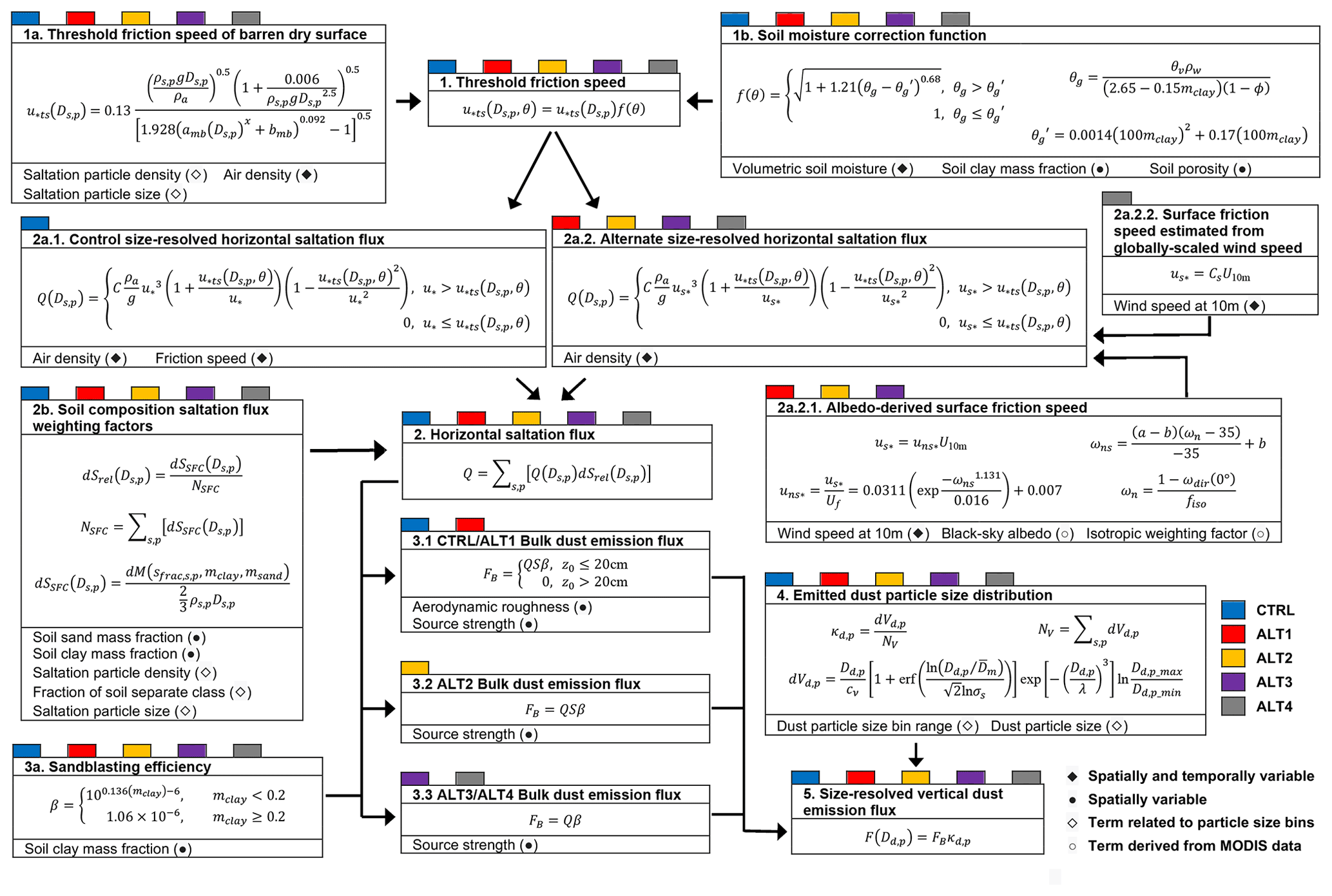
Figure 6Schematic of the original and modified components of the dust emission module and their required inputs. A black diamond indicates that the parameter varies spatially and temporally. A black circle indicates that the parameter varies spatially but not temporarily, and a hollow diamond means the term is related to a particle size bin attribute table. The hollow circle indicates that the field is derived from MODIS data. These input parameters are provided to the AFWA dust emission module by the WRF-Chem model. Color boxes imply which module components are used in the five different test configurations. See the comprehensive variable list in Table A1 for variable definitions.
Note that β, in this case, is homogenous in the study area (e.g., Fig. 4f) due to the relatively clay-rich soil content of the region (e.g., Fig. 4b) and is capped at 1.06 × 10⁻⁶ cm−1 everywhere the soil composition exceeds 20 % clay content (e.g., Fig. 4c). Accordingly, we can assume that the resultant simulated dust emission patterns produced by our test configurations are a function of Q, S, the z0 mask, or some combination of these parameters.
2.4 Observation data
We evaluated model performance using in situ observations from Automated Surface Observing Stations (ASOS). ASOS observations are available in standard Meteorological Aerodrome Report (METAR) format (e.g., WMO, 2019) every hour and in the less conventional 1 min or 5 min format, depending on the station. Gallagher et al. (2022) previously assessed model wind speed for our simulation configuration in the vicinity of the main event convection using 1 min frequency ASOS data. Thus, our analysis primarily focused on comparing simulated data against ASOS present weather and visibility observations as well as wind speed measurements for ambient conditions away from the main convective dust event using ASOS data accessed through the Meteorological Assimilation Data Ingest System (MADIS) portal (https://madis.ncep.noaa.gov, last access: 12 November 2021). We also compared simulated results against observed concentrations of particulate matter up to 10 µm in diameter (PM10) using hourly PM10 in situ measurements obtained from the US Environmental Protection Agency's Air Quality System database (retrieved via an application programming interface at https://www.epa.gov/outdoor-air-quality-data, last access: 1 July 2020). We did not consult additional satellite-retrieved products like false color dust-enhanced imagery and aerosol optical depth to supplement our assessment due to cloud obscuration over the area of interest.
To evaluate simulated storm structure, location, and timing, we analyzed observed Next Generation Weather Radar (NEXRAD) composite imagery (available at https://mesonet.agron.iastate.edu/docs/nexrad_mosaic/, last access: 2 February 2023) to qualitatively compare and verify the location, structure, and intensity of the simulated convective storms. The radar composite images comprise a blend of radar reflectivity from individual locations with overlapping coverage to generate a cohesive radar map across the continental United States. This mosaic approach has the advantage of filling in blockages from individual radar sites with neighboring ones, providing a more complete snapshot of convective activity across the radar network coverage area.
Experimental results are reviewed as follows. We begin with an overview of the uns* field, then review the environmental forcing conditions and dynamic components of the dust emission scheme simulated by the model. Lastly, we assess the resultant dust-related parameters produced by each test configuration outlined in Table 4. This holistic component-based approach helps to break down how the many factors affecting modeled dust conditions contributed to each test simulation outcome.
3.1 Albedo-derived normalized surface friction speed
Figure 7 shows the normalized surface wind friction speed for the case study period diagnosed from MODIS BRDF data and Eq. (11) interpolated to the model domain. Although we consider uns* to be a dynamic parameter, uns* here is a static field (i.e., uns* only varies spatially, not temporally) due to the relatively short duration of our case study simulation (48 h). Note that the uns* values in the areas characterized by the model as shrubland range from 0.0225 to 0.0325, barren areas are around 0.03 to 0.035, croplands are 0.0125 to 0.02, and forested and urban areas generally range from 0.005 to 0.0225. The upper limits of uns* associated with forested and urban areas are likely higher than those of croplands due to roughness element height consistency and density. For example, plants in individual crop fields generally grow at relatively uniform rates and spacing, giving the crop canopy a “smoother” aerodynamic roughness than urban centers and forested regions with more heterogeneity in roughness element height, shape, and density.
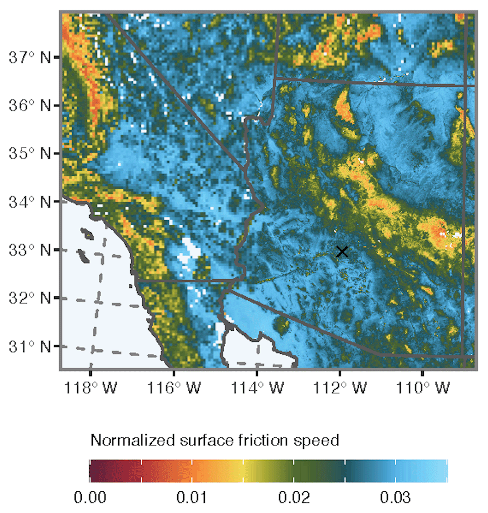
Figure 7Normalized surface friction speed (uns*) diagnosed from MODIS data. Due to the relatively short duration of our case study event, the uns* field remains fixed throughout the simulation. The black × marks the location of Phoenix, Arizona.
3.2 Environmental forcing conditions
We conducted a rigorous evaluation of the simulated environmental forcing conditions so we could account for any wind flow errors in our assessment of simulated PM10 against hourly station-based PM10 measurements. The model was able to reproduce the storm's general structure and timing, including the formation of the initial quasi-linear convective system and the collapse of the convective line into individual cells (results consistent with findings by Gallagher et al., 2022). Furthermore, the simulated near-surface wind speeds were in good agreement with wind speeds observed at ASOS. However, simulated wind speeds peaked 1 to 2 h early in some locations with slightly higher (about +1 m s−1) intensity. According to Gallagher et al. (2022), these minor wind speed errors may be partly due to erroneous land use characterization, particularly in the higher terrain elevation areas where the storm initiated. Gallagher et al. (2022) also performed a full statistical analysis of simulated surface wind speeds against all available ASOS wind speed data from the innermost domain (D03). The average wind speed bias for the entire forecast period was +0.59 m s−1. However, a large portion of this overestimation occurred during non-convective nocturnal periods (3 July at 05:00–15:00 UTC and 4 July at 08:00–16:00 UTC).
To better assess the potential influence of these minor errors in wind flow on simulated dust concentrations, we conducted a more in-depth review of the location and timing of the primary cell that produced the main dust event. Specifically, we examined locational differences between a central point along the storm's leading edge in both the observed and modeled radar reflectivity over the dust-producing cell's lifetime (Fig. 8). Overall, the simulated convective activity developed and propagated more northwest than the patterns we observed in the composite radar images. This divergence began with a slight difference in where the cells initiated, followed by a more prevalent westward motion in the simulated conditions than the storm's actual southwestern track. As the storm's evolution continued, the simulated event maintained its path and velocity, while the observed event pivoted and accelerated. Though variation between the simulated and actual storm tracks occurred, this distance became smaller over time (Fig. 8c).
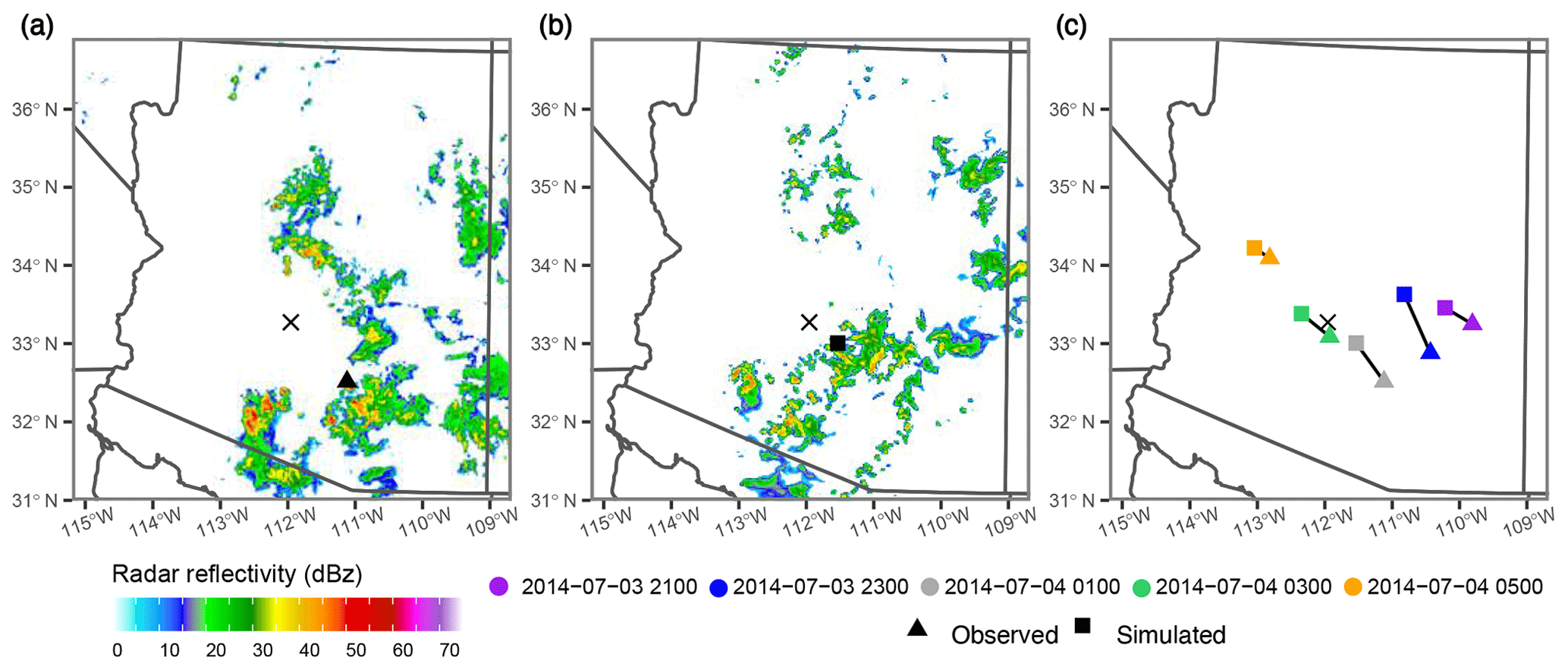
Figure 8Observed and simulated radar reflectivity for 4 July 2014 at 01:00 UTC, including an (a) observed composite radar image and (b) the model-simulated radar image. The black × marks the location of Phoenix, Arizona. Triangle and square markers indicate the location of a central point along the leading edge of the convective cell that affected Phoenix in the observed and simulated storms, respectively. The plot on the right (c) shows how these leading-edge central point locations evolved over time. Marker colors denote time in UTC.
Due to these discrepancies, we must limit our simulated dust assessment to a qualitative evaluation of the overall storm system rather than comparing hourly simulated time series of PM10 to observed values associated with an exact geospatial point. This approach, however, is not inconsistent with convective weather analyses since simulating the precise placement and timing of individual convective cells is generally considered more luck than skill due to irreducible limitations in nonlinear model physics, numerical processing, and initialization accuracy. Capturing the general spatial pattern and timing of the dust event is the higher priority as model users can often correct persistent magnitude errors through global model tuning parameters.
Simulated time series of U10 m, u*, and albedo-derived us* values associated with the peak of the dust event (4 July 2014, 00:00–03:00 UTC) are provided in Fig. 9. Overall, the U10 m patterns align well with the ASOS observations and areas of convective activity seen in the radar composite imagery (see Fig. S1 in the Supplement). We note that the simulated u* values are generally an order of magnitude stronger than their associated us* partition. This outcome is likely due to the drag partitioning scheme interpreting the relatively “dark” terrain surfaces of the domain landscape (presumably caused by the prevalence of shrubs and grasses or trees) as areas with substantial roughness element coverage.
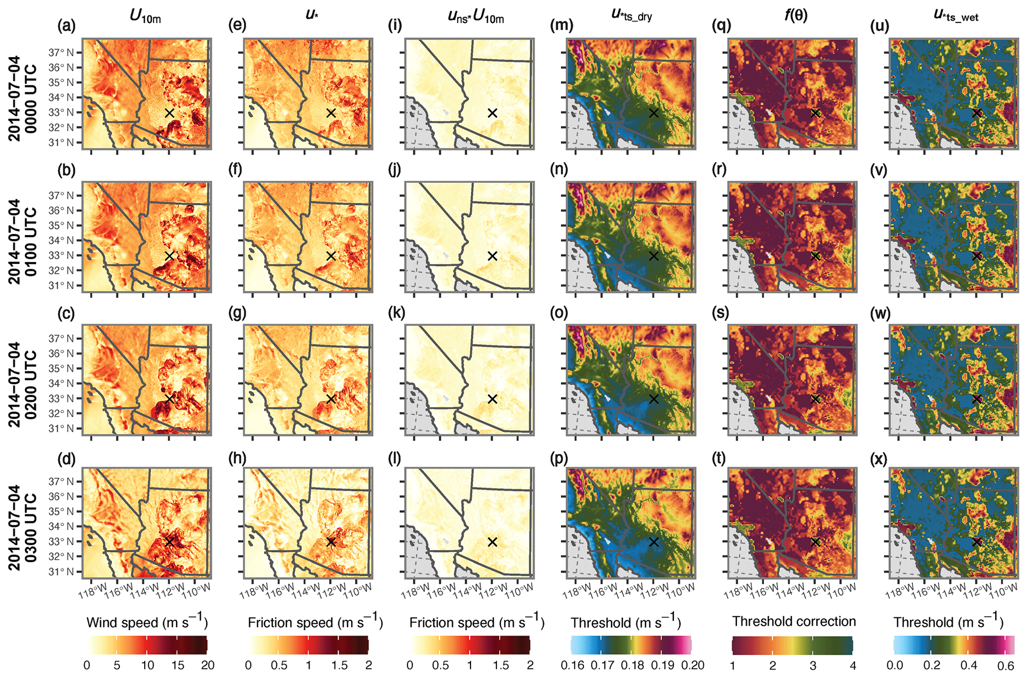
Figure 9Times series of simulated (a–d) 10 m wind speed (U10 m; m s−1), (e–h) total wind friction speed (u*; m s−1), (i–l) surface friction speed determined from the albedo-based drag parameterization (us*; m s−1), (m–p) threshold friction speed for a 69 µm diameter particle for an idealized smooth, dry, and barren soil surface ( µm); m s−1), (q–t) the soil-moisture-based correction function (f(θ); dimensionless), (u–x) and soil-wetness-corrected threshold friction speed for a 69 µm diameter particle ( µm, θ); m s−1) from 00:00 to 03:00 UTC on 4 July 2014. The u*ts_dry and u*ts_wet symbols used in the figure labeling represent µm) and ( µm, θ), respectively. The wetness-corrected threshold is the product of the threshold friction speed and the soil-moisture-based correction function. Note the differences in color bar scaling. The black × marks the location of Phoenix, Arizona.
Figure 9 also shows time series of the threshold friction speed for air-dry soil conditions, the soil-moisture-based correction function, and the soil-wetness-corrected threshold friction speed for a particle with a diameter of 69 µm ( µm), f(θ), and µm, θ), respectively). This particular particle size is the effective diameter for saltation size bin 7 (see Table 1). As described in a review paper by Kok et al. (2012, and references within), the u*ts parameter represents the minimum surface wind shear stress needed to overcome the inertial, cohesive, and adhesive forces holding the particle to the soil bed. Interparticle forces (e.g., capillary, Van der Waals, electrostatic, chemical binding, and Coulomb forces) keeping the particles fixed to the ground have a stronger effect on smaller particles due to their high ratio of surface area to volume. However, larger particles require more energy from the wind to mobilize because inertial force effects become stronger with increasing particle mass. The curve produced by Eq. (2) has a minimum of about 74 µm (assuming standard atmospheric pressure with 1.225 kg m−3 air density) because fine sand grains are less subject to interparticle forces than smaller clay- and silt-sized particles but are still relatively lightweight. Hence, fine sand-sized particles tend to be the first particles to mobilize from direct wind shear stress. Accordingly, particles associated with saltation size bin 7 ( µm) in the AFWA module will be the first to mobilize. Thus, we consider spatial patterns related to saltation size bin 7 to be good diagnostic indicators of overall dust emission model behavior.
Air density is the only spatiotemporally varying parameter in the calculation of . Though we can discern a slight reduction in µm) over time immediately under the convective line (Fig. 9m–p), the overall effect of air density on for this case is relatively negligible. Under air-dry soil conditions, µm) ranges between 0.17 and 0.19 m s−1 across most of the domain. These results also align with findings by Darmenova et al. (2009) in their assessment of the sensitivity of the Marticorena and Bergametti (1995) dust emission scheme to uncertainties in its required input parameters.
We also see relatively little change in the f(θ) field during the dust event, except for the area associated with a line of precipitation that occurred within the convective cell behind the main wall of dust (Fig. 9q–t). The µm, θ) maxima over the Mogollon Rim align with isolated areas of convective precipitation that occurred earlier in the simulation (Fig. 9u–x). Note, however, that the µm, θ) values along the Mogollon Rim adjacent to these maxima are around 0.2 to 0.3 m s−1, comparable to µm, θ) values in the southwestern Arizona region where the dust event occurred and, for the most part, well below the simulated values of u*. This particular aspect of the model behavior is important because the only component of the AFWA module preventing dust emissions from these drier forested areas in the ALT3 and ALT4 simulations is the drag partition treatment.
Figure 10 shows time series of the excess friction speed, u*ex, for saltation size bin 7 associated with different treatments for particle mobilization during the peak of the event, where u*ex is the model simulated friction speed driving the saltation and dust emission equations (i.e., u* or us*) minus µm, θ). The six examples provided in Fig. 10 include u*ex calculated using the model-generated u* values, us* values derived using the Chappell and Webb (2016) method (Eq. 1), and four instances of us* values estimated from 10 m wind speeds scaled by a global tuning constant (Cs; Eq. 14) as the wind forcing parameter. We considered values of Cs=0.02, 0.025, 0.03, and 0.035 based on the general range of uns* values diagnosed for the area where the dust event occurred (e.g., Fig. 7; note that uns* has a theoretical maximum of 0.0381). Effectively, positive u*ex values indicate that wind friction speeds are strong enough in the model to initiate particle mobilization, while negative u*ex values imply that the wind friction speeds are too weak. Immediately, we see that practically the entire domain is capable of lofting dust in the u*-driven simulations if sufficient dust and saltator material are present (Fig. 10a–d). Conversely, dust production in the us*-driven simulations is restricted to isolated areas, including areas near the leading edges of individual storm cells (e.g., Fig. 10e–x). The u*ex results generated with globally scaled U10 m and Cs=0.025 (Fig. 10e–h) are markedly similar to the u*ex values calculated with U10 m scaled by uns* (Fig. 10q–t). In particular, the excess friction speeds for these two instances match rather closely over Arizona, with minor spatial extent differences for positive u*ex values in California and southern Nevada. Thus, we chose Cs=0.025 as the U10 m global scaling constant for our ALT4 test configuration. Interestingly, areas in the uns* field equal to 0.025 (Fig. 7) tend to align with grid cells characterized as closed shrubland (Fig. 3) in the model domain where there were strong winds, though this may be a coincidence.
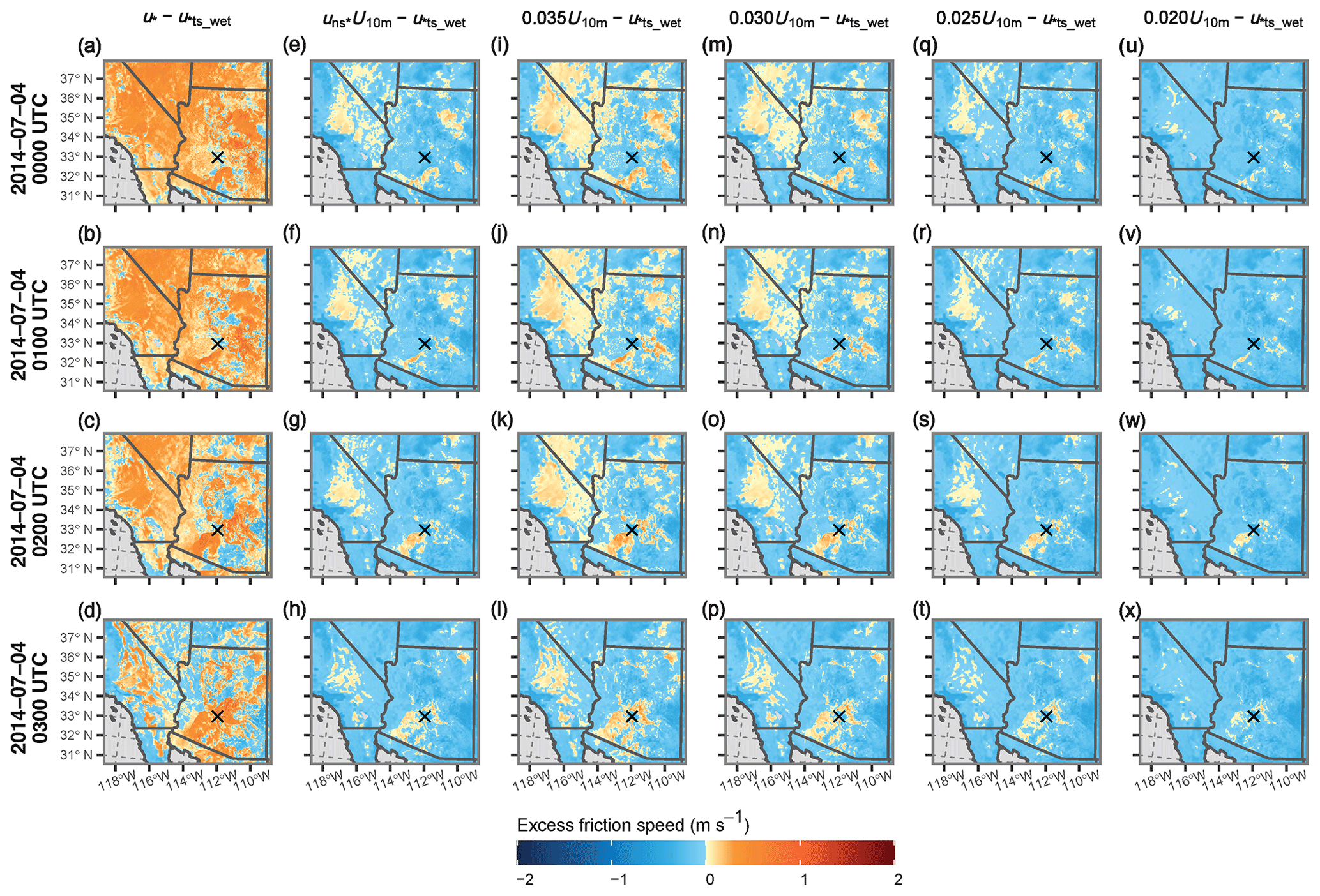
Figure 10Times series of excess friction speed (u*ex; (u*ex; m s−1) calculated by subtracting the friction speed for a 69 µm diameter particle, µm, θ), from the wind forcing parameter driving dust production from 00:00 to 03:00 UTC on 4 July 2014. The u*ts_wet symbol used in the figure labeling represents µm, θ). Plots provided include (a–d) u*ex calculated using total friction speed, (e–h) surface friction speed determined from the albedo-based drag parameterization, and (i–x) four instances of 10 m wind speeds scaled using a global tuning constant as the wind forcing parameter. The black × marks the location of Phoenix, Arizona.
To further explore how our code modifications influenced simulated outcomes, we diagnosed time series of the horizontal saltation flux for the peak of the dust event associated with each test configuration (Fig. 11). Though the non-erodible area masking components of the AFWA dust emission code are not applied in the AFWA module until the FB calculation (Eq. 6), we included the appropriate non-erodible area masks for the CTRL, ALT1, and ALT2 configurations (see Fig. 5) in the Fig. 11 Q diagnostics. Strong saltation occurred everywhere in the CTRL configuration plots unless the grid spaces were masked out (e.g., Fig. 11a–d). The four alternative model configurations showed Q patterns similar to each other, suggesting that the masking had little influence on the resultant Q flux in AFWA module configurations that accounted for drag partition. The ALT1 and ALT2 Q outcomes were practically identical because the z0>20 cm mask largely coincides with the areas where S=0 for this domain (e.g., Fig. 5). With the exception of a small area of saltation to the east of Phoenix, the ALT3 Q results are also similar to ALT1 and ALT2, which makes sense as developed and urban areas as well as higher-elevation forested regions generally yield low values of uns*. Lastly, the ALT4 Q spatial patterns mimic ALT3. However, the magnitude of the ALT4 Q flux in the areas outside where the main dust event occurred is lower than the ALT1, ALT2, and ALT3 results.
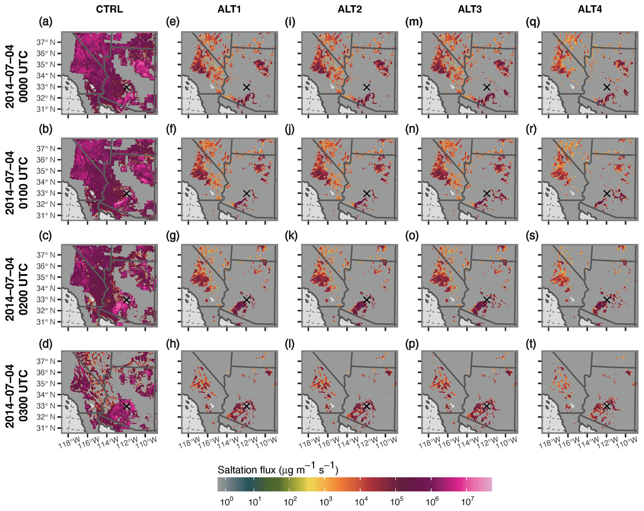
Figure 11Times series of horizontal saltation flux (Q; µg m−1 s−1) for each test configuration (CTRL, ALT1, ALT2, ALT3, and ALT4) with non-erodible area masking applied from 00:00 to 03:00 UTC on 4 July 2014. The black × marks the location of Phoenix, Arizona.
3.3 Simulated dust conditions
We compared our simulation results against observed PM10 concentrations (Figs. 12–14). To ensure our simulated PM10 conditions could primarily be attributed to dust transport, we also reviewed the general contribution of each aerosol species to the overall simulated PM10 patterns (not pictured). For this case, most of the simulated PM10 came from either dust or sea salt transport. Sea salt and dimethyl sulfide distributions were relatively isolated to areas over the ocean and the immediate coastlines, while dust was the primary source of PM10 over land. Contributions from black carbon, organic carbon, and dimethyl sulfide to simulated PM10 totals were negligible, except in dense urban areas along the southern California coastline.
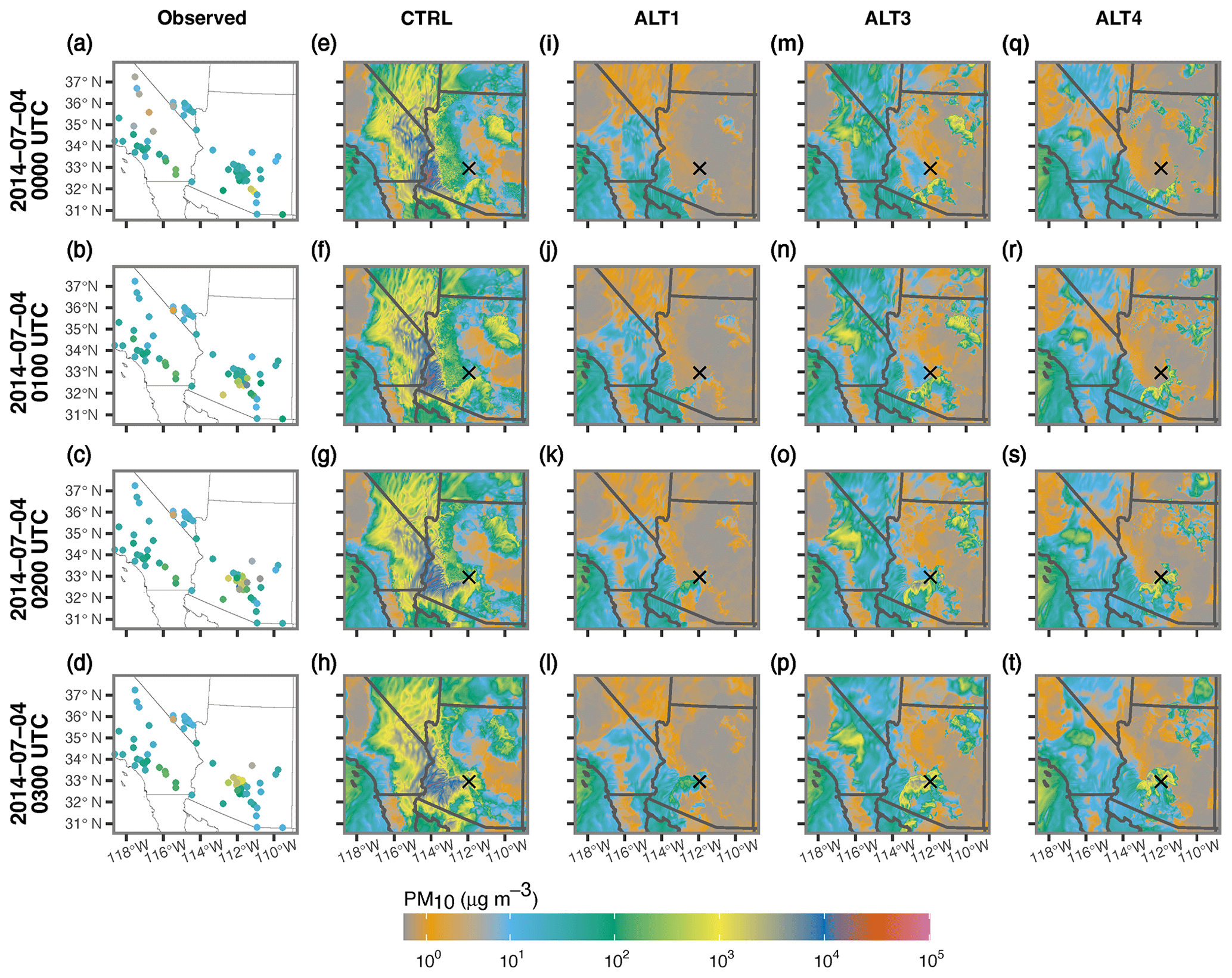
Figure 12Times series of observed and simulated PM10 concentration for each test configuration (CTRL, ALT1, ALT3, and ALT4) (µg m−3) from 00:00 to 03:00 UTC on 4 July 2014. The black × marks the location of Phoenix, Arizona. The ALT2 configuration results are not included in this figure since they are nearly identical to results from the ALT1 configuration.
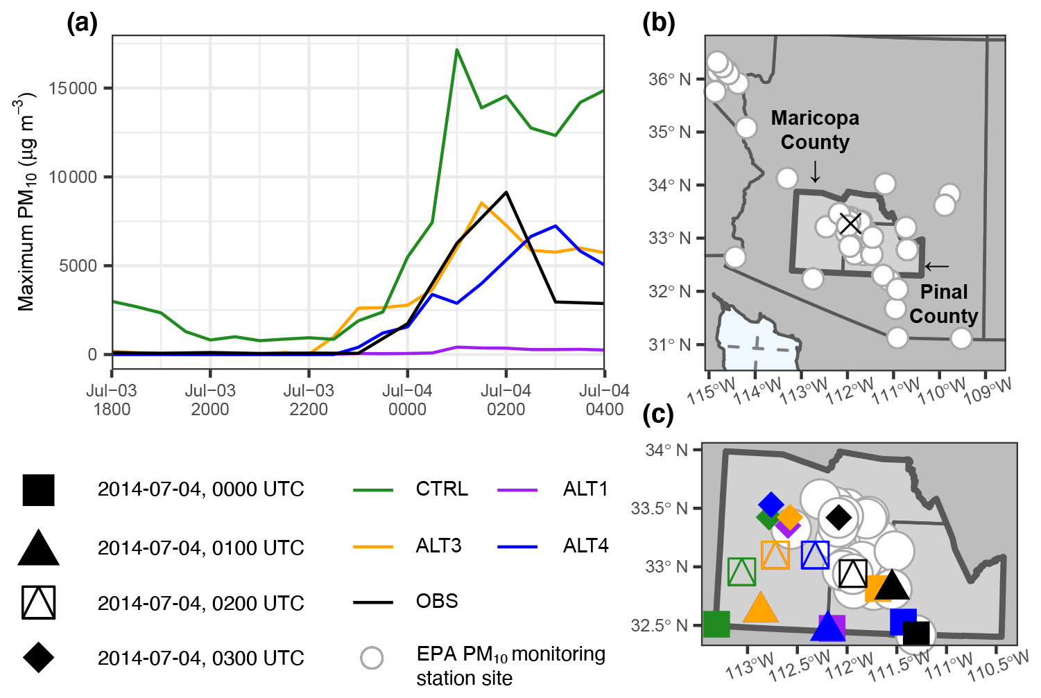
Figure 13(a) Time series of observed (OBS) and simulated (CTRL, ALT1, ALT3, and ALT4) maximum PM10 concentration (µg m−3) for the combined Maricopa and Pinal counties in Arizona. Panel (b) highlights how most EPA monitoring stations in Arizona are in Maricopa county and Pinal county, clustered around the Phoenix metropolitan area (marked by the black ×). We used the hourly maximum PM10 concentrations from the combined Maricopa and Pinal county areas for our assessment due to the shifted nature of the main dust-producing outflow boundary recorded by the EPA stations situated around Phoenix, Arizona, in the simulations. The map zoom in (c) of the Maricopa county and Pinal county boundaries shows the EPA station locations relative to the hourly PM10 maximum values sampled for each test configuration and the observations on 4 July 2014 from 00:00–03:00 UTC. The ALT2 configuration results are not included in this figure since they are nearly identical to results from the ALT1 configuration. Note that the CTRL, ALT1, and ALT3 PM10 maximum value sites overlap on 4 July 2014 at 01:00 UTC, and the ALT1 and ALT3 sites are co-located on 4 July 2014 at 02:00 UTC.
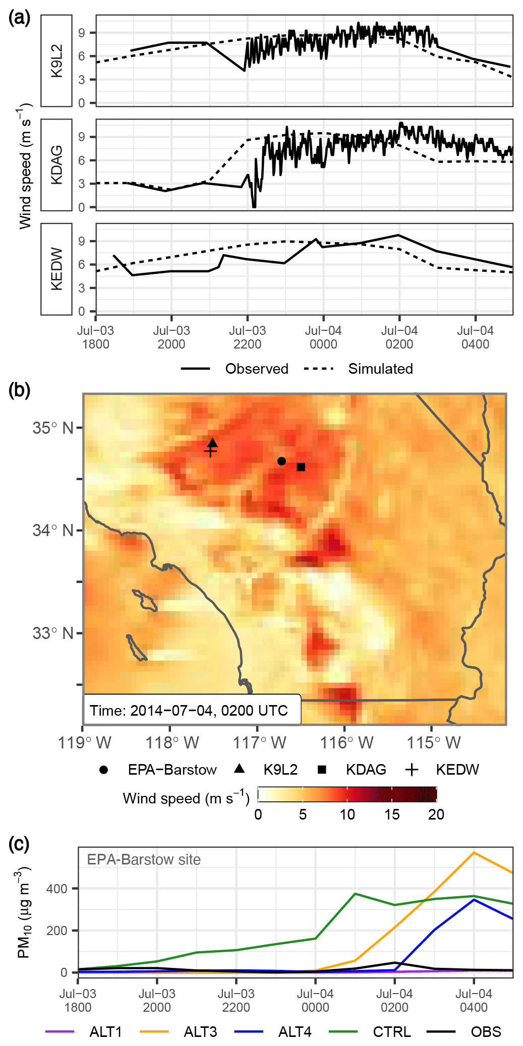
Figure 14Simulated and observed (a) surface wind speed and (c) PM10 values for ASOS and EPA station locations in the Mojave Desert area associated with the erroneously simulated PM10 plume. The spatial plot (b) shows the station locations relative to the area of maximum wind speed simulated by the model over the Mojave Desert on 4 July 2014 at 02:00 UTC, when observed PM10 values for the general location peaked.
Note that PM10 monitoring stations in the United States are generally situated around populated areas, so most of the PM10 sites associated with our model domain were tightly clustered around Phoenix (e.g., Fig. 13b). The dust wall crossed over the Phoenix metropolitan area between 00:00 and 04:00 UTC on 4 July 2014. Importantly, the air quality conditions rapidly recovered once the main dust wall passed, and the areas outside the immediate dust event were relatively clear. According to surface weather station visibility, present weather records, and observer remarks for Arizona and southern California (not pictured), it is unlikely the strong dust obscurations extended much beyond the immediate convective cell outflow boundary area.
The original CTRL configuration produced a strong dust signal along the convective outflow boundary, but it also generated widespread dust concentrations in areas that in reality were clear (e.g., Fig. 12). Similar to the Q flux patterns, simulated PM10 concentrations produced by the ALT1 and ALT2 configurations were nearly identical because dust in the us*-driven simulations did not originate near a masked area (see Fig. 5). Due to this artifact, we opted to limit our PM10 assessment to the CTRL, ALT1, ALT3, and ALT4 simulations. The ALT1 configuration produced much lower PM10 concentrations than the other test settings, with some dust emerging near the gust front. The ALT1 “dust wall”, however, was an order of magnitude lower than the observed conditions. In contrast, the magnitude and spatial pattern of the simulated PM10 values associated with ALT3 and ALT4 aligned better with reported observations.
Though the general PM10 patterns of the main dust event are similar between ALT3 and ALT4, the areas of maximum PM10 extend further south along the gust front in the ALT3 simulation than in the ALT4 version (Fig. 12). We also note higher PM10 values for ALT3 in southern California over the Mojave Desert and near the northeastern corner of Arizona compared to ALT4. However, the maximum PM10 values associated with these two areas occurred in observation-limited regions. PM10 observations from an EPA station in Barstow, California (site ID: 06-071-0001; 34.8939080∘ N 117.024804∘ W), near the simulated area of maximum PM10 over the Mojave Desert suggest that simulated PM10 values in both ALT3 and ALT4 were higher than observed at this location (Fig. 14c). For example, simulated PM10 values for ALT3 and ALT4 at the Barstow site peaked at 570 and 346 µg m−3, respectively, at 00:00 UTC on 4 July 2014, while observed PM10 values ranged between 5 and 47 µg m−3 during the 4 July 2014 00:00–04:00 UTC period. However, the PM10 concentrations in the simulations changed rapidly over short distances near the Barstow EPA station as the simulations evolved. Thus, small shifts in the simulated dust position could greatly affect the apparent skill of the simulated output.
Surface wind speed observations from Edwards Air Force Base (KEDW, K9L2), which is primarily upstream and west of the simulated Mojave Desert PM10 plume, and Barstow (KDAG) suggest that there were strong wind speeds over the area in question (Fig. 14). Observed wind speeds at the Barstow ASOS station closest to the simulated PM10 plume ranged from ∼ 5 to 10 m s−1 between 00:00 and 03:00 UTC on 4 July 2014, which aligns relatively well with the modeled 10 m wind speeds. Though the simulated wind speed ramp-up for the Barstow location was slightly early on 3 July 2014, the observed strong winds persisted longer over a similar time span before decaying. Accordingly, we can conclude that the model reproduced a realistic wind evolution pattern over the Mojave Desert. While the actual dust conditions for the area are less clear, the lack of commentary about dust in the recorded ASOS observer remarks leads us to believe that the simulated PM10 values for both the ALT3 and ALT4 configurations in the Mojave Desert region were higher than what occurred. However, the cause of this discrepancy is unclear. The erroneous PM10 feature could be due to issues with the drag partition treatment, unresolved sediment supply influences, a combination of the two factors, or some other source of error within the model.
Though we are unable to do point-specific quantitative evaluations for the Phoenix metropolitan area due to the shifted location of the main dust-producing outflow boundary in the simulations, we can see from our spatial PM10 time series analysis (e.g., Fig. 12) that the maximum PM10 value during the peak of the dust event was generally co-located with the storm outflow boundary. Thus, we compared the simulated maximum PM10 values for the area surrounding Phoenix with the maximum PM10 values observed by the EPA stations as the dust wall passed over the city. Figure 13 shows time series of observed and simulated maximum PM10 concentration for the combined Maricopa and Pinal counties in Arizona. This combined county area generally encompasses the footprint of both the simulated and observed track of the storm. Note that the gust front in the simulation advanced into the combined county area earlier than the recorded event (see Fig. 8), and the main dust wall moved away from the EPA stations around Phoenix after 03:00 UTC. Therefore, we expect the simulated combined county maximum PM10 values to be higher than the observed PM10 conditions before and after the observed PM10 peak at 02:00 UTC on 4 July 2014. During the 00:00 to 03:00 UTC period, the observed maximum PM10 was 9132 µg m−3, while the CTRL, ALT1, ALT3, and ALT4 configurations produced maximum PM10 values for the combined county area of 17 151, 419, 8539, and 7240 µg m−3, respectively. If we emphasize the order of magnitude over the exact value of PM10 from these results to account for observed and simulated gust front location differences, both ALT3 and ALT4 produced reasonable results.
Findings from this case study show that incorporating a drag partition treatment into the AFWA dust emission module can improve simulated dust transport for vegetated dryland regions. The CTRL simulation results with no drag partitioning align with previous findings that the default AFWA module settings produce excessive dust conditions in the southwestern United States. While the albedo-based drag partition method improved the results with respect to PM10 spatial patterns and concentration magnitudes, we also achieved similar outcomes with a global wind scaling parameter.
We argue that the ALT4 globally scaled wind speed approach, at least how it is applied in our case study, should also be considered a crude form of drag partitioning. However, unlike the Chappell and Webb (2016) method, this global drag partitioning approach assumes that the effects of the variability in vegetation cover over the dust-producing areas within the model domain are relatively negligible for the dust entrainment process. Our case study results imply that the spatial variability of uns* was not a key factor in the evolution of the dust storm simulation, but this outcome may simply be an artifact of the conditions associated with our chosen case study. This particular dust event occurred in a confined, localized area due to its convective nature over a shrub-dominated landscape with relatively homogenous topography (e.g., Figs. 2–3). The spatial variability of uns* in the broader region may have more influence on dust events generated by synoptically driven wind forcing conditions (i.e., horizontal length scales on the order of several hundred kilometers to 1000+ km). Furthermore, the ALT4 configuration does not provide a viable modeling solution for users interested in exploring the effects of land management or land cover change on sediment transport and air quality and may be limited in its use to short-term atmospheric forecasting applications.
It appears that drag partition treatments effectively suppressed the broad-scale erroneous dust emissions in southern California and southwestern Arizona inherent to the CTRL configuration without restricting the dust emissions that generated the Phoenix haboob. However, the relatively low PM10 concentrations produced by the ALT1 simulation suggest that the S parameter was masking the absence of drag representation in the original AFWA code. Although the model performance for this case study is arguably better with the drag partition when S=1, this may not be the case for all regions. Further investigation of the role of the S parameter in areas with more heterogeneous sediment supply is necessary to resolve this issue.
In order to better isolate the role of the uns* spatial heterogeneity in our results from the effects of soil moisture on the dust emission process, we reproduced the diagnostic excess friction speed time series from Fig. 10 but used the threshold friction speed for air-dry soil conditions for saltation size bin 7 instead of the moisture-corrected threshold value (u*ex_dry; Fig. 15). The resultant u*ex_dry values for all wind forcing treatments are, at least to some degree, largely higher in magnitude than their moisture-corrected counterparts in Fig. 10. However, both the u*ex and u*ex_dry values for the forested areas along the Mogollon Rim are generally low, even when using values for Cs that align with the albedo-derived uns* estimates associated with the barren and shrubland areas. For example, the uns* values for the forested Mogollon Rim region in Fig. 7 are primarily less than 0.02 throughout the peak of the dust event. This suggests that model sensitivity for this domain to the albedo-based drag partition may vary for alternate wind flow conditions and that the albedo-based drag partition scheme could potentially benefit from additional validation studies.
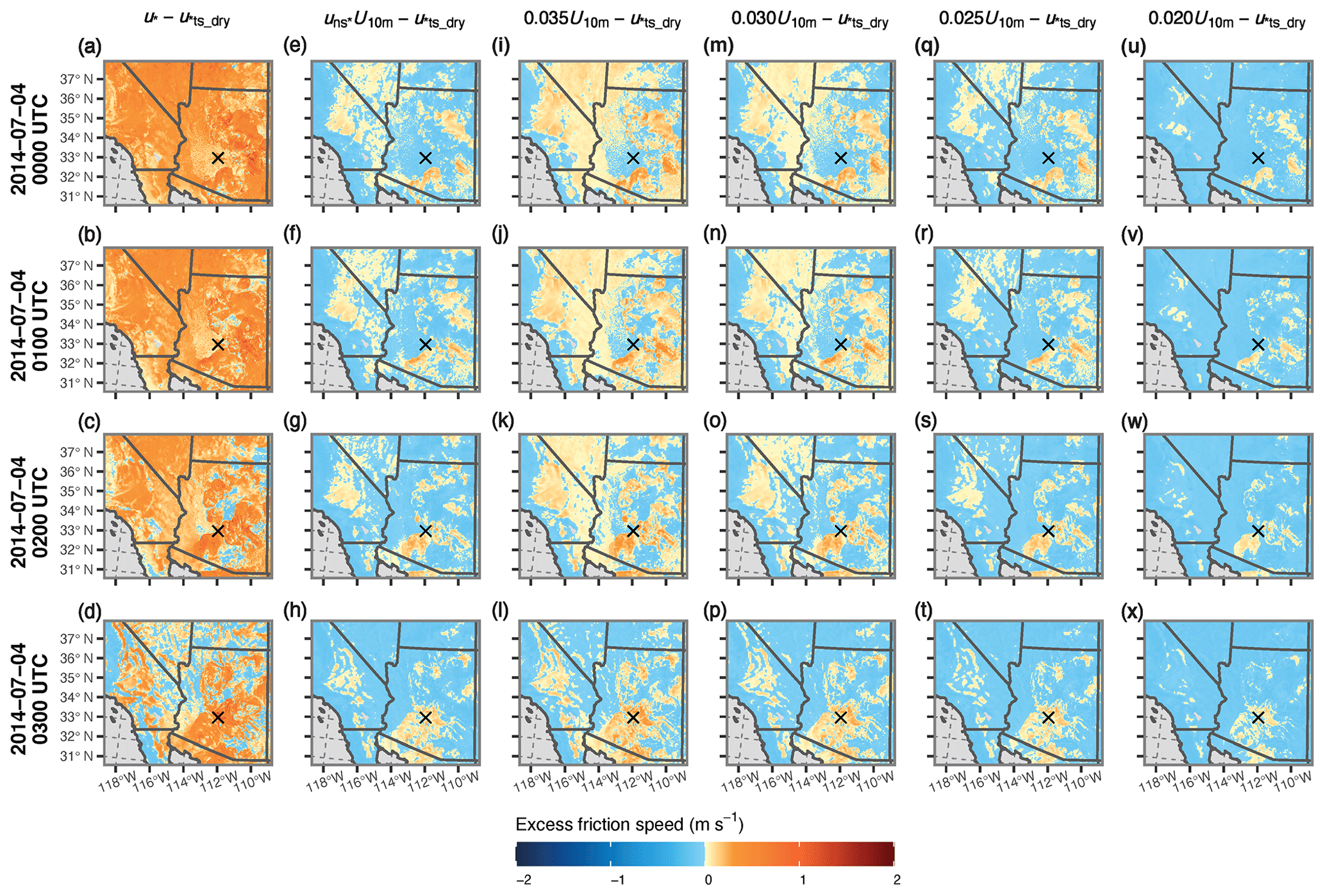
Figure 15Times series of excess friction speed (u*ex; m s−1) calculated by subtracting the friction speed for a 69 µm diameter particle, µm, θ), from the wind forcing parameter driving dust production from 00:00 to 03:00 UTC on 4 July 2014. The u*ts_wet symbol used in the figure labeling represents µm, θ). Plots provided include (a–d) u*ex calculated using total friction speed, (e–h) surface friction speed determined from the albedo-based drag parameterization, and (i–x) four instances of 10 m wind speeds scaled using a global tuning constant as the wind forcing parameter. The black × marks the location of Phoenix, Arizona. Excess friction speed (u*ex_dry; m s−1) calculated by subtracting the dry threshold friction speed for a 69 µm diameter particle, µm), from the wind forcing parameter driving dust production from 00:00 to 03:00 UTC on 4 July 2014. The u*ex_dry symbol used in the figure labeling represents µm). Plots provided include (a–d) excess friction speed calculated using total friction speed, (e–h) surface friction speed determined from the albedo-based drag parameterization, and (i–x) four instances of 10 m wind speeds scaled using a global tuning constant as the wind forcing parameter. The black × marks the location of Phoenix, Arizona.
We note, however, that modeled 10 m wind speeds will be reduced over forested areas due to the aerodynamic drag from the trees on simulated wind speeds and that these particular aerodynamic roughness effects vary as a function of the z0 settings in the parent WRF model. The drag partition treatment, at least with respect to how it is configured in our modeling setup, has no influence on simulated winds outside the dust emission calculation. Even if the uns* values were high for a model grid cell with forest cover, the simulated winds would likely be reduced by the internal WRF model physics, potentially mitigating (or masking) a shortfall in the drag partition correction.
These peculiar results over the forested area also highlight the need for consistency of aerodynamic roughness treatments between the dust emission module and other components of the parent weather model, including the land surface and planetary boundary layer schemes, so that u* and us* diagnosed for the dust emission treatment are consistent with the other model elements governing simulated wind flow. Findings by Webb et al. (2014b) demonstrate how these kinds of inconsistencies can lead to erroneously modeled increases in sediment transport with increasing vegetation coverage. As dust emission models like the AFWA module are further refined, careful consideration should be taken when configuring model components that incorporate land surface conditions on aerodynamic processes.
Even though we were able to largely replicate the PM10 case study simulations produced with the albedo-based drag partition by using a global scaling factor, it is important to remember that our Cs value selection was informed by the albedo-derived uns* values and that the relatively short duration of our case study event meant that the uns* values associated with our study were static throughout the event life cycle. In any event, choosing an appropriate Cs value a priori could be challenging when using the globally scaled surface wind speed approach for operational forecasting, climatological applications, or a larger domain with more variability in vegetation coverage over dust-producing areas.
Spatial uns* patterns derived from MODIS data will likely evolve over longer time spans from processes like annual vegetation growth cycles, drought conditions, anomalous wet periods, and land cover change. To investigate, we reviewed the temporal coefficient of variation (CV) of 500 m gridded monthly mean snow-masked uns* values in our case study area over the 2001–2021 MODIS record (Fig. 16) and found that CV values generally ranged between 1 % and 12 % for grid pixels in the dust-producing regions of southwestern Arizona, with a few clusters of pixels ranging between 15 % and 20 % over active agricultural areas. By comparison, with the global Cs drag partitioning (ALT4), we saw markedly different spatial patterns in areas of the model domain capable of initiating saltation simply by varying the Cs parameter by increments of 0.005 (e.g., Figs. 10 and 15), or %. Given that uns* and Cs are mathematically equivalent with respect to the model implementation (i.e., in terms of being multiplied by U10 m to generate us* in Eqs. 1 and 14, respectively), our MODIS-derived uns* CV analysis suggests that Cs=0.025 may be a reasonable setting for this domain in general. Nonetheless, though these CV values may appear to indicate a relatively low amount of variability in MODIS-derived uns* over the majority of the dust-producing region, even modest changes in uns* may result in simulated us* values exceeding or falling below u*ts.

Figure 16The spatiotemporal variability of uns* for the 2001–2021 MODIS record shown as the coefficient of variation of monthly uns* as a percentage. The black × marks the location of Phoenix, Arizona. Note that the color bar tick marks increase in increments of 5 % after the 30 % mark.
Thus, the degree to which the observed variability in uns* matters from a mesoscale dust modeling context is still unclear. Okin (2005) explored the influence of surface heterogeneity on saltation flux following the original method of Raupach et al. (1993), whereby the drag partition adjusts u*ts directly rather than modifying the u* value driving the saltation flux equation. When reviewing the daily saltation flux as a function of the CV of u*ts, Okin (2005) found that CV values of 10 % or less produced minimal differences in saltation flux. Additional modeling case studies focused on seasonal and interannual land cover changes are needed to determine the sensitivity of the AFWA dust emission module to uns* variability.
Based on these findings, we argue that the Chappell and Webb (2016) drag partition approach may have the potential to improve dust transport model performance in vegetated dryland regions. Still, it is worth discussing the nuances associated with its use. On the one hand, the technique removes the dependence on greenness-related remote sensing indicators. By using albedo in a way that is interpreted as shadow to discern roughness elements and their associated aerodynamic properties, the Chappell and Webb (2016) technique may capture the drag induced by plants as well as drag generated by engineered and natural structures like fences, tillage furrows, and subgrid-scale topographic relief. In theory, this method incorporates subgrid-scale heterogeneity and temporal variability in its calculation.
Another aspect to consider is the use of 10 m wind speed in Eq. (1), which is not physically based. The original derivation for us* multiplied uns* by a parameter Chappell and Webb (2016) referred to as “the free-stream wind speed” or Uf (also referred to by some studies as Uh). Yet this Uf parameter is not associated with wind speed in the free atmosphere (i.e., wind speed above the atmospheric boundary layer). Instead, the value stems from the free-stream flow associated with the wind tunnel data collected by Marshall (1971) that Chappell and Webb (2016) used to develop their equations, which has no direct replacement. Additional research is needed to assess the degree of error introduced by the Uf=U10 m assumption.
The Chappell and Webb (2016) scheme also assumes that all observed shadows emanate from solid subgrid-scale roughness objects within the flow field. This assumption could be obviated if shadows cast by tall objects extend into neighboring grid cells, creating a sensitivity to wind direction. While this is not likely to be an issue at the mesoscale or coarser modeling scales with uns* values derived from 500 m MODIS data, additional lower-bound grid-resolution limitation studies may be necessary before applying the Chappell and Webb (2016) drag partition method to finer-scale dust transport models (e.g., large eddy simulation and field-scale models) with uns* initialized from high-fidelity data sources.
Like many other parameterizations, the Chappell and Webb (2016) drag partition is empirical. It incorporates multiple rounds of normalization and draws conclusions about nature from idealized “black-sky” (i.e., 100 % direct illumination) scenarios that do not exist in real-world settings. Furthermore, the Marshall (1971) wind tunnel experiments that Chappell and Webb (2016) used to establish their drag partition equations used non-porous, rigid cylinders to imitate natural roughness elements. Multiple studies have since demonstrated that the cylinder method is often a poor representation the aerodynamic behavior of live vegetation (e.g., Walter et al., 2012). Arguably, the effects of uncertainties in the rescaling parameters associated with the albedo approach on simulated dust entrainment outcomes may be comparable to errors created by uncertainties in inputs and configuration parameters required for other drag partition methods. Additional studies comparing the many available drag partitioning approaches in mesoscale and global-scale dust transport models over extended periods of vegetation green-up and senescence are needed to fully resolve this issue.
Given the relative simplicity of implementing the Chappell and Webb (2016) drag partition into dust emission modeling code, it would be worthwhile to continue investigating use of the scheme in convection-permitting and regional-scale dust transport models. At these scales, many of the aforementioned issues would likely be small or negligible compared to errors introduced by other parts of the modeling framework that govern u* and erodible sediment supply. In fact, some US agencies have already begun to incorporate the Chappell and Webb (2016) drag partition into their operational air quality models (e.g., Tong et al., 2020).
Finally, though the MODIS data preprocessing steps required by the Chappell and Webb (2016) drag partition are comparable to the processing requirements of other air quality and weather model input datasets, operational environmental prediction agencies may find the additional processing burden prohibitive. The computational resource allocations of production systems often operate near capacity in order to meet a multitude of simulation parameter output requirements and data dissemination schedules, making it challenging to justify added data ingest and preprocessing steps for a single model parameter. Accordingly, future efforts could explore the feasibility of using monthly or seasonal climatologies of uns* for weather forecasting applications.
This study explored the use of an albedo-based drag partitioning scheme introduced by Chappell and Webb (2016) to incorporate roughness effects into a widely used dust emission and transport model within WRF-Chem. Our results for a convective dust event case study for the desert region around Phoenix, Arizona, support previous findings that the original WRF-Chem/GOCART/AFWA model configuration is prone to producing widespread erroneous dust emissions in the southwestern United States. Furthermore, our findings suggest that incorporating a drag partition treatment into the AFWA dust emission module may improve dust transport simulation and forecasting in vegetated dryland regions through better sheltering-effect representation on dust emissions. This code adaptation could take the form of a formal drag partition treatment or a wind speed tuning approach if the roughness element coverage of the dust-producing areas associated with the model domain is somewhat homogenous and the simulation is run over a short enough period that the surface roughness configuration does not change. We note, however, that we cannot generalize model performance from a single case study event. Instead, we view this study as a preliminary demonstration of capability and motivation to further explore the use of drag partitioning in dust transport models to account for roughness effects on the dust entrainment process. Additional case studies and seasonal analyses are necessary to determine if the Chappell and Webb (2016) drag partition method can reliably improve dust simulations used for various weather prediction, land management, and climate change modeling applications.
The benefits of using a drag partition methodology in the AFWA module are manifest in the vast improvements we see with ALT3 and ALT4 over the initial CTRL configuration. Follow-on studies are still necessary to explore if these benefits persist over longer simulation periods. However, we anticipate that satellite-derived roughness information could markedly improve investigations of the role of short- and long-term changes in vegetation in dust emission patterns. This, in turn, could be of benefit to model users interested in drought hazard, climate change, land management, land use and land cover change, and post-wildfire condition modeling applications.
Table A1 provides the symbol, name, units, and value or description of variables referred to throughout this paper. Values of prescribed constants are listed. Variable arrays are described as “variable” for size-bin-related settings, “spatially varying parameter” for static fields, and “spatiotemporally varying parameter” for temporally dynamic fields. See Fig. 6 for a schematic overview of how these parameters are used in the AFWA module calculations.
Table A1Variable list. Units are provided in terms of mass [M], length [L], and time [T]. In the Type column, “C” implies the parameter is a prescribed constant or global scaling factor, “V” indicates the parameter is a prescribed one-dimensional array of size-bin-related settings, “SV” parameters are spatially varying static fields, and “STV” parameters are spatiotemporally varying dynamic fields.
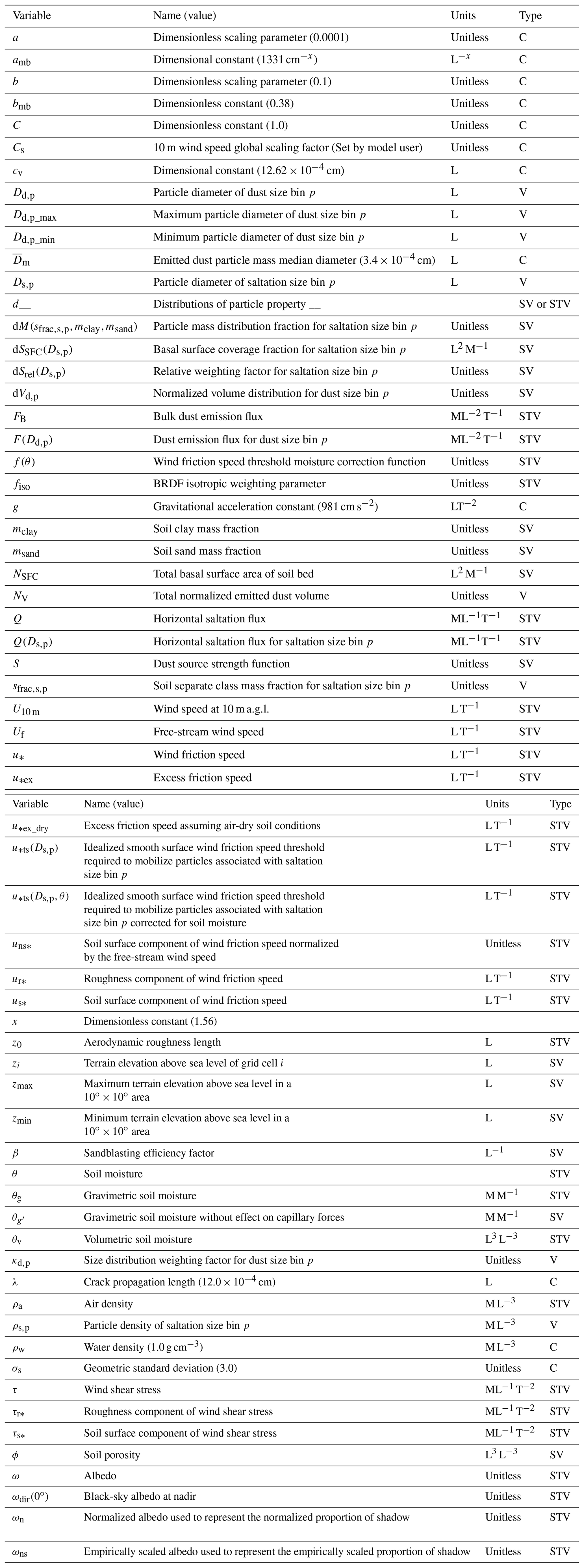
WRF-Chem v4.1 baseline source code and run instructions are available for download at https://github.com/wrf-model/WRF/releases/tag/v4.1 (NCAR, 2019, last access: 1 June 2020). The modified version of WRF-Chem v4.1 used to produce the results described in this paper is available for download via Zenodo (https://doi.org/10.5281/zenodo.7447886, Letcher et al., 2022). This modified source code includes additional runtime-activated functions that allow users to easily switch between the original AFWA dust emission module settings (i.e., CTRL) and the alternate configurations with drag partition included (i.e., ALT1, ALT2, ALT3, and ALT4). The Zenodo repository also includes a copy of the WRF Pre-processing System v4.2 code used to prepare the terrain and forcing data for our case study simulations. Detailed modified code descriptions, guidance for preparing the MODIS uns* input data, and model runtime instructions are thoroughly documented in the report by Michaels et al. (2022).
The MODIS albedo datasets required for calculating the drag partition are available from the NASA EOSDIS Land Processes DAAC portal, including the daily BRDF isometric weighting parameter (https://doi.org/10.5067/MODIS/MCD43A1.061, Schaaf and Wang, 2021a) and the daily black sky albedo (https://doi.org/10.5067/MODIS/MCD43A3.061, Schaaf and Wang, 2021b) for MODIS band 1. Data for creating the MODIS snow mask can be obtained from the NASA National Snow and Ice Data Center (https://doi.org/10.5067/MODIS/MOD10A1.006, Hall and Riggs, 2016). All model-forcing data used in this study can be obtained from the National Centers for Environmental Information Archive Information Request System (AIRS). Rapid Refresh analysis data can be downloaded via https://www.ncei.noaa.gov/products/weather-climate-models/rapid-refresh-update (NOAA National Centers for Environmental Information, 2023a), and North American Model Analysis fields are available at https://www.ncei.noaa.gov/products/weather-climate-models/north-american-mesoscale (NOAA National Centers for Environmental Information, 2023b). The minute frequency ASOS data considered for this study are available at https://www.ncei.noaa.gov/data/automated-surface-observing-system-one-minute-pg1/access/2014/07/ (NOAA National Weather Service, 2005). Archived global hourly ASOS data for 2014 can be downloaded at https://www.ncei.noaa.gov/data/global-hourly/archive/csv/2014.tar.gz (NOAA National Centers for Environmental Information, 2001). However, we recommend readers procure the July 2014 hourly ASOS data from the Meteorological Assimilation Data Ingest System (MADIS) portal at https://madis.ncep.noaa.gov (last access: 12 November 2021) to avoid having to download the entire 2014 global record.. Archived hourly PM10 data can be retrieved via an application programming interface at https://www.epa.gov/outdoor-air-quality-data (US Environmental Protection Agency, 2022). Archived Next Generation Weather Radar (NEXRAD) composite imagery data sets in raster format are available for download at https://mesonet.agron.iastate.edu/docs/nexrad_mosaic/ (Iowa Environmental Mesonet, 2023).
The supplement related to this article is available online at: https://doi.org/10.5194/gmd-16-1009-2023-supplement.
SLL developed the project concept and experimental design, performed the majority of the data analysis and interpretation with in collaboration with GSO and NPW, served as the primary paper author, and led project efforts. SD provided the MODIS-derived uns* input datasets. TWL and MLM modified the WRF-Chem code to implement the albedo drag partition into the AFWA module and produced the WRF-Chem case study simulation data. ARG, SLL, TSH, and TWL conducted the gust front location offset assessment. SD performed the uns* CV analysis. NPZ assisted with writing and concept development. All co-authors critically reviewed the paper.
The contact author has declared that none of the authors has any competing interests.
Publisher's note: Copernicus Publications remains neutral with regard to jurisdictional claims in published maps and institutional affiliations. Any use of trade, product, or firm names is for descriptive purposes only and does not imply endorsement by the US Government. Permission to publish was granted by the ERDC Geospatial Research Laboratory. The USDA is an equal opportunity provider and employer.
The authors thank Yongkang Xue and Yongwei Sheng for their insightful comments and technical discussions. The authors also wish to thank their pets for being loyal writing companions.
This research has been supported by the US Army Engineer Research and Development Center (project no. 479378, Extreme Terrain Research: “Forecasting EO/IR Extinction Characteristics for Active and Passive Optical Systems”), NASA ROSES (grant no. 80NSSC20K1673), and NIH (grant no. R01AI48336).
This paper was edited by Havala Pye and reviewed by two anonymous referees.
Adams, D. K. and Comrie, A. C.: The North American Monsoon, B. Am. Meteorol. Soc., 78, 2197–2213, https://doi.org/10.1175/1520-0477(1997)078<2197:TNAM>2.0.CO;2, 1997. a
Aragnou, E., Watt, S., Duc, H. N., Cheeseman, C., Riley, M., Leys, J., White, S., Salter, D., Azzi, M., Chang, L. T.-C., Morgan, G., and Hannigan, I.: Dust transport from inland Australia and its impact on air quality and health on the eastern coast of Australia during the February 2019 dust storm, Atmosphere, 12, 141, https://doi.org/10.3390/atmos12020141, 2021. a
Asadov, Kh. G. and Kerimov, N. I.: On the necessity of correction of the methodology for calculating aerosol flux from the Earth’s surface to the atmosphere using the NDVI index, Fundamental and Applied Climatology, 3, 92–101, https://doi.org/10.21513/2410-8758-2019-3-92-101, 2019 (in Russian). a
Benjamin, S. G., Weygandt, S. S., Brown, J. M., Hu, M., Alexander, C. R., Smirnova, T. G., Olson, J. B., James, E. P., Dowell, D. C., Grell, G. A., Lin, H., Peckham, S. E., Smith, T. L., Moninger, W. R., Kenyon, J. S., and Manikin, G. S.: A North American hourly assimilation and model forecast cycle: The Rapid Refresh, Mon. Weather Rev., 144, 1669–1694, https://doi.org/10.1175/MWR-D-15-0242.1, 2016. a
Bukowski, J. and van den Heever, S. C.: The impact of land surface properties on haboobs and dust lofting, J. Atmos. Sci., 79, 3195–3218, https://doi.org/10.1175/JAS-D-22-0001.1, 2022. a
Cakmur, R. V., Miller, R. L., Perlwitz, J., Geogdzhayev, I. V., Ginoux, P., Koch, D., Kohfeld, K. E., Tegen, I., and Zender, C. S.: Constraining the magnitude of the global dust cycle by minimizing the difference between a model and observations, J. Geophys. Res., 111, D06207, https://doi.org/10.1029/2005JD005791, 2006. a
Chappell, A. and Webb, N. P.: Using albedo to reform wind erosion modelling, mapping and monitoring, Aeolian Res., 23, 63–78, https://doi.org/10.1016/j.aeolia.2016.09.006, 2016. a, b, c, d, e, f, g, h, i, j, k, l, m, n, o, p, q, r, s, t, u, v, w, x, y
Chappell, A., Van Pelt, S., Zobeck, T., and Dong, Z.: Estimating aerodynamic resistance of rough surfaces using angular reflectance, Remote Sens. Environ., 114, 1462–1470, https://doi.org/10.1016/j.rse.2010.01.025, 2010. a
Chin, M., Rood, R. B., Lin, S.-J., Müller, J.-F., and Thompson, A. M.: Atmospheric sulfur cycle simulated in the global model GOCART: Model description and global properties, J. Geophys. Res.-Atmos., 105, 24671–24687, https://doi.org/10.1029/2000JD900384, 2000. a
Collins, W. J., Bellouin, N., Doutriaux-Boucher, M., Gedney, N., Halloran, P., Hinton, T., Hughes, J., Jones, C. D., Joshi, M., Liddicoat, S., Martin, G., O'Connor, F., Rae, J., Senior, C., Sitch, S., Totterdell, I., Wiltshire, A., and Woodward, S.: Development and evaluation of an Earth-System model – HadGEM2, Geosci. Model Dev., 4, 1051–1075, https://doi.org/10.5194/gmd-4-1051-2011, 2011. a
Cremades, P. G., Fernández, R. P., Allende, D. G., Mulena, G. C., and Puliafito, S. E.: High resolution satellite derived erodibility factors for WRF/Chem windblown dust simulations in Argentina, Atmósfera, 30, 11–25, https://doi.org/10.20937/ATM.2017.30.01.02, 2017. a
Darmenova, K., Sokolik, I. N., Shao, Y., Marticorena, B., and Bergametti, G.: Development of a physically based dust emission module within the Weather Research and Forecasting (WRF) model: Assessment of dust emission parameterizations and input parameters for source regions in Central and East Asia, J. Geophys. Res., 114, D14201, https://doi.org/10.1029/2008JD011236, 2009. a, b
Ek, M. B., Mitchell, K. E., Lin, Y., Rogers, E., Grunmann, P., Koren, V., Gayno, G., and Tarpley, J. D.: Implementation of Noah land surface model advances in the National Centers for Environmental Prediction operational mesoscale Eta model, J. Geophys. Res.-Atmos., 108, 8851, https://doi.org/10.1029/2002JD003296, 2003. a
Evans, S., Ginoux, P., Malyshev, S., and Shevliakova, E.: Climate‐vegetation interaction and amplification of Australian dust variability, Geophys. Res. Lett., 43, 11823–11830, https://doi.org/10.1002/2016GL071016, 2016. a, b, c
Fast, J. D., Gustafson, W. I., Easter, R. C., Zaveri, R. A., Barnard, J. C., Chapman, E. G., Grell, G. A., and Peckham, S. E.: Evolution of ozone, particulates, and aerosol direct radiative forcing in the vicinity of Houston using a fully coupled meteorology-chemistry-aerosol model, J. Geophys. Res., 111, D21305, https://doi.org/10.1029/2005JD006721, 2006. a, b
Fécan, F., Marticorena, B., and Bergametti, G.: Parametrization of the increase of the aeolian erosion threshold wind friction velocity due to soil moisture for arid and semi-arid areas, Ann. Geophys., 17, 149–157, https://doi.org/10.1007/s00585-999-0149-7, 1999. a
Fountoukis, C., Ackermann, L., Ayoub, M. A., Gladich, I., Hoehn, R. D., and Skillern, A.: Impact of atmospheric dust emission schemes on dust production and concentration over the Arabian Peninsula, Model. Earth Syst. Environ., 2, 115, https://doi.org/10.1007/s40808-016-0181-z, 2016. a
Francis, D., Nelli, N., Fonseca, R., Weston, M., Flamant, C., and Cherif, C.: The dust load and radiative impact associated with the June 2020 historical Saharan dust storm, Atmos. Environ., 268, 118808, https://doi.org/10.1016/j.atmosenv.2021.118808, 2022. a
Freitas, S. R., Longo, K. M., Alonso, M. F., Pirre, M., Marecal, V., Grell, G., Stockler, R., Mello, R. F., and Sánchez Gácita, M.: PREP-CHEM-SRC – 1.0: a preprocessor of trace gas and aerosol emission fields for regional and global atmospheric chemistry models, Geosci. Model Dev., 4, 419–433, https://doi.org/10.5194/gmd-4-419-2011, 2011. a
Fu, L.-T.: Comparisons suggest more efforts are required to parameterize wind flow around shrub vegetation elements for predicting aeolian flux, Sci. Rep., 9, 3841, https://doi.org/10.1038/s41598-019-40491-z, 2019. a
Gallagher, A. R., LeGrand, S. L., Hodgdon, T. S., and Letcher, T. W.: Simulating environmental conditions for southwest United States convective dust storms using the Weather Research and Forecasting model v4.1, ERDC TR-22-11, U.S. Army Engineer Research and Development Center, Hanover, New Hampshire, USA, https://doi.org/10.21079/11681/44963, 2022. a, b, c, d, e, f, g, h, i
Gillette, D. A.: Fine particulate emissions due to wind erosion, Trans. Am. Soc. Agric. Eng., 20, 890–897, https://doi.org/10.13031/2013.35670, 1977. a
Ginoux, P., Chin, M., Tegen, I., Prospero, J. M., Holben, B., Dubovik, O., and Lin, S.-J.: Sources and distributions of dust aerosols simulated with the GOCART model, J. Geophys. Res., 106, 20255–20273, https://doi.org/10.1029/2000JD000053, 2001. a, b, c, d
Gong, S. L.: A parameterization of sea-salt aerosol source function for sub- and super-micron particles, Global Biogeochem. Cy., 17, 1097, https://doi.org/10.1029/2003GB002079, 2003. a
Grell, G. A., Peckham, S. E., Schmitz, R., McKeen, S. A., Frost, G., Skamarock, W. C., and Eder, B.: Fully coupled “online” chemistry within the WRF model, Atmos. Environ., 39, 6957–6975, https://doi.org/10.1016/j.atmosenv.2005.04.027, 2005. a, b
Hall, D. K. and Riggs, G. A.: MODIS/Terra Snow Cover Daily L3 Global 500 m Grid, Version 6, NASA National Snow and Ice Data Center Distributed Active Archive Center Boulder, Colorado USA [data set], https://doi.org/10.5067/MODIS/MOD10A1.006, 2016. a, b
Hamzeh, N. H., Karami, S., Kaskaoutis, D. G., Tegen, I., Moradi, M., and Opp, C.: Atmospheric dynamics and numerical simulations of six frontal dust storms in the Middle East region, Atmosphere, 12, 125, https://doi.org/10.3390/atmos12010125, 2021. a
Han, J. and Pan, H.-L.: Revision of convection and vertical diffusion schemes in the NCEP Global Forecast System, Weather Forecast., 26, 520–533, https://doi.org/10.1175/WAF-D-10-05038.1, 2011. a
Hyde, P., Mahalov, A., and Li, J.: Simulating the meteorology and PM10 concentrations in Arizona dust storms using the Weather Research and Forecasting model with Chemistry (Wrf-Chem), J. Air Waste Manage., 68, 177–195, https://doi.org/10.1080/10962247.2017.1357662, 2018. a, b, c
Iacono, M. J., Delamere, J. S., Mlawer, E. J., Shephard, M. W., Clough, S. A., and Collins, W. D.: Radiative forcing by long-lived greenhouse gases: Calculations with the AER radiative transfer models, J. Geophys. Res., 113, D13103, https://doi.org/10.1029/2008JD009944, 2008. a
Ito, A. and Kok, J. F.: Do dust emissions from sparsely vegetated regions dominate atmospheric iron supply to the Southern Ocean?, J. Geophys. Res.-Atmos., 122, 3987–4002, https://doi.org/10.1002/2016JD025939, 2017. a, b, c
Iowa Environmental Mesonet: Documentation on IEM generated NEXRAD Mosaics, N0R (4bit) Reflectivity, https://mesonet.agron.iastate.edu/docs/nexrad_mosaic/, last access: 2 February 2023.
Karumuri, R. K., Kunchala, R. K., Attada, R., Dasari, H. P., and Hoteit, I.: Seasonal simulations of summer aerosol optical depth over the Arabian Peninsula using WRF‐Chem: Validation, climatology, and variability, Int. J. Climatol., 42, 2901–2922, https://doi.org/10.1002/joc.7396, 2022. a
Kim, D., Chin, M., Bian, H., Tan, Q., Brown, M. E., Zheng, T., You, R., Diehl, T., Ginoux, P., and Kucsera, T.: The effect of the dynamic surface bareness on dust source function, emission, and distribution, J. Geophys. Res.-Atmos., 118, 871–886, https://doi.org/10.1029/2012JD017907, 2013. a, b
Kim, K., Kim, S., Choi, M., Kim, M., Kim, J., Shin, I., Kim, J., Chung, C., Yeo, H., Kim, S., Joo, S. J., McKeen, S. A., and Zhang, L.: Modeling Asian dust storms using WRF‐Chem during the DRAGON‐Asia Field Campaign in April 2012, J. Geophys. Res.-Atmos., 126, e2021JD034793, https://doi.org/10.1029/2021JD034793, 2021. a
King, J., Nickling, W. G., and Gillies, J. A.: Representation of vegetation and other nonerodible elements in aeolian shear stress partitioning models for predicting transport threshold, J. Geophys. Res.-Earth, 110, F04015, https://doi.org/10.1029/2004JF000281, 2005. a
Kok, J. F.: A scaling theory for the size distribution of emitted dust aerosols suggests climate models underestimate the size of the global dust cycle, P. Natl. Acad. Sci. USA, 108, 1016–1021, https://doi.org/10.1073/pnas.1014798108, 2011. a
Kok, J. F., Parteli, E. J. R., Michaels, T. I., and Karam, D. B.: The physics of wind-blown sand and dust, Rep. Prog. Phys., 75, 106901, https://doi.org/10.1088/0034-4885/75/10/106901, 2012. a, b
Kok, J. F., Albani, S., Mahowald, N. M., and Ward, D. S.: An improved dust emission model – Part 2: Evaluation in the Community Earth System Model, with implications for the use of dust source functions, Atmos. Chem. Phys., 14, 13043–13061, https://doi.org/10.5194/acp-14-13043-2014, 2014. a
Koven, C. D. and Fung, I.: Identifying global dust source areas using high-resolution land surface form, J. Geophys. Res., 113, D22204, https://doi.org/10.1029/2008JD010195, 2008. a
Kuchera, E. L., Rentschler, S. A., Creighton, G. A., and Rugg, S. A.: A review of operational ensemble forecasting efforts in the United States Air Force, Atmosphere, 12, 677, https://doi.org/10.3390/atmos12060677, 2021. a
LeGrand, S. L., Polashenski, C., Letcher, T. W., Creighton, G. A., Peckham, S. E., and Cetola, J. D.: The AFWA dust emission scheme for the GOCART aerosol model in WRF-Chem v3.8.1, Geosci. Model Dev., 12, 131–166, https://doi.org/10.5194/gmd-12-131-2019, 2019. a, b, c, d, e, f, g, h, i, j
Letcher, T. W. and LeGrand, S. L.: A comparison of simulated dust produced by three dust-emission schemes in WRF-Chem: Case study assessment, ERDC/CRREL TR-18-13, U.S. Army Engineer Research and Development Center, Hanover, New Hampshire, USA, https://doi.org/10.21079/11681/28868, 2018. a
Letcher, T. W., LeGrand, S. L., and Michaels, M. L.: WRF-Chem-v4.1-AFWA-Drag-Partition-Modifications: Full model code release (bug-fix release) (v1.1.1), Zenodo [code], https://doi.org/10.5281/zenodo.7447886, 2022. a, b
Li, J., Okin, G. S., Herrick, J. E., Belnap, J., Miller, M. E., Vest, K., and Draut, A. E.: Evaluation of a new model of aeolian transport in the presence of vegetation, J. Geophys. Res.-Earth, 118, 288–306, https://doi.org/10.1002/jgrf.20040, 2013. a
Ma, S., Zhang, X., Gao, C., Tong, D. Q., Xiu, A., Wu, G., Cao, X., Huang, L., Zhao, H., Zhang, S., Ibarra-Espinosa, S., Wang, X., Li, X., and Dan, M.: Multimodel simulations of a springtime dust storm over northeastern China: implications of an evaluation of four commonly used air quality models (CMAQ v5.2.1, CAMx v6.50, CHIMERE v2017r4, and WRF-Chem v3.9.1), Geosci. Model Dev., 12, 4603–4625, https://doi.org/10.5194/gmd-12-4603-2019, 2019. a
Marshall, J. K.: Drag measurements in roughness arrays of varying density and distribution, Agric. Meteorol., 8, 269–292, https://doi.org/10.1016/0002-1571(71)90116-6, 1971. a, b, c
Marticorena, B. and Bergametti, G.: Modeling the atmospheric dust cycle: 1. Design of a soil-derived dust emission scheme, J. Geophys. Res., 100, 16415, https://doi.org/10.1029/95JD00690, 1995. a, b, c
Mayaud, J. and Webb, N.: Vegetation in drylands: Effects on wind flow and aeolian sediment transport, Land, 6, 64, https://doi.org/10.3390/land6030064, 2017. a
Mesbahzadeh, T., Salajeghe, A., Sardoo, F. S., Zehtabian, G., Ranjbar, A., Marcello Miglietta, M., Karami, S., and Krakauer, N. Y.: Spatial-temporal variation characteristics of vertical dust flux simulated by WRF-Chem model with GOCART and AFWA dust emission schemes (Case study: Central Plateau of Iran), Appl. Sci., 10, 4536, https://doi.org/10.3390/app10134536, 2020. a
Michaels, M. L., Letcher, T. W., LeGrand, S. L., Webb, N. P., and Putnam, J. B.: Implementation of an albedo-based drag partition into the WRF-Chem v4.1 AFWA dust emission module, ERDC/CRREL TR-22-2, U.S. Army Engineer Research and Development Center, Hanover, New Hampshire, USA, https://doi.org/10.21079/11681/42782, 2022. a, b, c
Miller, P. W., Williams, M., and Mote, T.: Modeled atmospheric optical and thermodynamic responses to an exceptional Trans‐Atlantic dust outbreak, J. Geophys. Res.-Atmos., 126, e2020JD032909, https://doi.org/10.1029/2020JD032909, 2021. a
Mohebbi, A., Green, G. T., Akbariyeh, S., Yu, F., Russo, B. J., and Smaglik, E. J.: Development of dust storm modeling for use in freeway safety and operations management: An Arizona case study, Transp. Res. Rec. J. Transp. Res. Board, 2673, 175–187, https://doi.org/10.1177/0361198119839978, 2019. a
Mohebbi, A., Yu, F., Cai, S., Akbariyeh, S., and Smaglik, E. J.: Spatial study of particulate matter distribution, based on climatic indicators during major dust storms in the State of Arizona, Front. Earth Sci., 15, 133–150, https://doi.org/10.1007/s11707-020-0814-4, 2020. a
Nabavi, S. O., Haimberger, L., and Samimi, C.: Sensitivity of WRF-chem predictions to dust source function specification in West Asia, Aeolian Res., 24, 115–131, https://doi.org/10.1016/j.aeolia.2016.12.005, 2017. a
Nakanishi, M. and Niino, H.: An improved Mellor–Yamada Level-3 Model with condensation physics: Its design and verification, Boundary Layer Meteorol., 112, 1–31, https://doi.org/10.1023/B:BOUN.0000020164.04146.98, 2004. a, b
National Center for Atmospheric Research (NCAR): WRF Version 4.1, Github [code], https://github.com/wrf-model/WRF/releases/tag/v4.1 (last access: 1 June 2020), 2019. a
Nguyen, H. D., Riley, M., Leys, J., and Salter, D.: Dust storm event of February 2019 in Central and East Coast of Australia and evidence of long-range transport to New Zealand and Antarctica, Atmosphere, 10, 653, https://doi.org/10.3390/atmos10110653, 2019. a
Nikfal, A., Raadatabadi, A., and Sehatkashani, S.: Investigation of dust schemes in the model WRF/Chem, J. Air Pollut. Health, 3, 1–8, 2018. a
NOAA National Centers for Environmental Information: Global Surface Hourly [ASOS Hourly Data: 2014] [data set], NOAA National Centers for Environmental Information, https://www.ncei.noaa.gov/data/global-hourly/archive/csv/2014.tar.gz (last access: 2 February 2023), 2001.
NOAA National Centers for Environmental Information: Rapid Refresh/Rapid Update Cycle, https://www.ncei.noaa.gov/products/weather-climate-models/rapid-refresh-update, last access: 1 February 2023a.
NOAA National Centers for Environmental Information: North American Mesoscale Forecast System, https://www.ncei.noaa.gov/products/weather-climate-models/north-american-mesoscale, last access: 1 February 2023b.
NOAA National Weather Service U.S. Federal Aviation Administration, U.S. Department of Defense, and NOAA National Centers for Environmental Information: 1-Minute Page 1 Surface Weather Observations from the Automated Surface Observing Systems (ASOS) Network, [July 2014] [data set], NOAA National Centers for Environmental Information, NCEI DSI 6405_02, https://www.ncei.noaa.gov/data/automated-surface-observing-system-one-minute-pg1/access/2014/07/ (last access: 12 November 2021), 2005.
Okin, G. S.: Dependence of wind erosion and dust emission on surface heterogeneity: Stochastic modeling, J. Geophys. Res., 110, D11208, https://doi.org/10.1029/2004JD005288, 2005. a, b
Okin, G. S.: A new model of wind erosion in the presence of vegetation, J. Geophys. Res., 113, F02S10, https://doi.org/10.1029/2007JF000758, 2008. a, b
Okin, G. S.: The contribution of brown vegetation to vegetation dynamics, 91, 743–755, https://doi.org/10.1890/09-0302.1, 2010. a
Parajuli, S. P. and Zender, C. S.: Projected changes in dust emissions and regional air quality due to the shrinking Salton Sea, Aeolian Res., 33, 82–92, https://doi.org/10.1016/j.aeolia.2018.05.004, 2018. a, b
Parajuli, S. P., Stenchikov, G. L., Ukhov, A., and Kim, H.: Dust emission modeling using a new high‐resolution dust source function in WRF‐Chem with implications for air quality, J. Geophys. Res.-Atmos., 124, 10109–10133, https://doi.org/10.1029/2019JD030248, 2019. a
Parajuli, S. P., Stenchikov, G. L., Ukhov, A., Shevchenko, I., Dubovik, O., and Lopatin, A.: Aerosol vertical distribution and interactions with land/sea breezes over the eastern coast of the Red Sea from lidar data and high-resolution WRF-Chem simulations, Atmos. Chem. Phys., 20, 16089–16116, https://doi.org/10.5194/acp-20-16089-2020, 2020. a
Peckham, S. E., Grell, G., McKeen, S. A., Ahmadov, R., Wong, K. Y., Barth, M., Pfister, G., Wiedinmyer, C., Fast, J. D., Gustafson, W. I., Ghan, S. J., Zaveri, R., Easter, R. C., Barnard, J., Chapman, E., Hewson, M., Schmitz, R., Salzmann, M., Beck, V., and Freitas, S. R.: WRF-Chem version 3.8.1 user’s guide, NOAA Technical Memorandum OAR GSD-48, 83 pp., https://doi.org/10.7289/V5/TM-OAR-GSD-48, 2017. a
Péré, J.-C., Rivellini, L., Crumeyrolle, S., Chiapello, I., Minvielle, F., Thieuleux, F., Choël, M., and Popovici, I.: Simulation of African dust properties and radiative effects during the 2015 SHADOW campaign in Senegal, Atmos. Res., 199, 14–28, https://doi.org/10.1016/j.atmosres.2017.07.027, 2018. a
Pierre, C., Bergametti, G., Marticorena, B., Kergoat, L., Mougin, E., and Hiernaux, P.: Comparing drag partition schemes over a herbaceous Sahelian rangeland: Drag partitions comparison in Sahel, J. Geophys. Res.-Earth, 119, 2291–2313, https://doi.org/10.1002/2014JF003177, 2014. a
Raupach, M. and Lu, H.: Representation of land-surface processes in aeolian transport models, Environ. Modell. Softw., 19, 93–112, https://doi.org/10.1016/S1364-8152(03)00113-0, 2004. a
Raupach, M. R.: Drag and drag partition on rough surfaces, Bound.-Lay. Meteorol., 60, 375–395, https://doi.org/10.1007/BF00155203, 1992. a
Raupach, M. R., Gillette, D. A., and Leys, J. F.: The effect of roughness elements on wind erosion threshold, J. Geophys. Res.-Atmos., 98, 3023–3029, https://doi.org/10.1029/92JD01922, 1993. a, b, c
Rizza, U., Anabor, V., Mangia, C., Miglietta, M. M., Degrazia, G. A., and Passerini, G.: WRF-Chem simulation of a Saharan dust outbreakover the Mediterranean regions, Ciência e Natura, 38, 330–336, https://doi.org/10.5902/2179460X20249, 2016. a
Rizza, U., Kandler, K., Eknayan, M., Passerini, G., Mancinelli, E., Virgili, S., Morichetti, M., Nolle, M., Eleftheriadis, K., Vasilatou, V., and Ielpo, P.: Investigation of an intense dust outbreak in the Mediterranean using XMed-Dry Network, multiplatform observations, and numerical modeling, Appl. Sci., 11, 1566, https://doi.org/10.3390/app11041566, 2021. a
Saidou Chaibou, A. A., Ma, X., Kumar, K. R., Jia, H., Tang, Y., and Sha, T.: Evaluation of dust extinction and vertical profiles simulated by WRF-Chem with CALIPSO and AERONET over North Africa, J. Atmos. Sol.-Terr. Phy., 199, 105213, https://doi.org/10.1016/j.jastp.2020.105213, 2020. a
Saleeby, S. M., van den Heever, S. C., Bukowski, J., Walker, A. L., Solbrig, J. E., Atwood, S. A., Bian, Q., Kreidenweis, S. M., Wang, Y., Wang, J., and Miller, S. D.: The influence of simulated surface dust lofting and atmospheric loading on radiative forcing, Atmos. Chem. Phys., 19, 10279–10301, https://doi.org/10.5194/acp-19-10279-2019, 2019. a
Schaaf, C. and Wang, Z.: MODIS/Terra+Aqua BRDF/Albedo Model Parameters Daily L3 Global – 500 m V061, NASA EOSDIS Land Processes DAAC [data set], https://doi.org/10.5067/MODIS/MCD43A1.061, 2021a. a, b
Schaaf, C. and Wang, Z.: MODIS/Terra+Aqua BRDF/Albedo Daily L3 Global – 500 m V061, NASA EOSDIS Land Processes DAAC [data set], https://doi.org/10.5067/MODIS/MCD43A3.061, 2021b. a, b
Shao, Y., Nickling, W., Bergametti, G., Butler, H., Chappell, A., Findlater, P., Gillies, J., Ishizuka, M., Klose, M., Kok, J. F., Leys, J., Lu, H., Marticorena, B., McTainsh, G., McKenna-Neuman, C., Okin, G. S., Strong, C., and Webb, N.: A tribute to Michael R. Raupach for contributions to aeolian fluid dynamics, Aeolian Res., 19, 37–54, https://doi.org/10.1016/j.aeolia.2015.09.004, 2015. a
Skamarock, W. C., Klemp, J. B., Dudhia, J., Gill, D. O., Liu, Z., Berner, J., Wang, W., Powers, J. G., Duda, M. G., Barker, D. M., and Huang, X.-Y.: A description of the Advanced Research WRF Model version 4, NCAR Technical Notes; NCAR/TN-556+STR, UCAR/NCAR, https://doi.org/10.5065/1DFH-6P97, 2019. a, b
Solomos, S., Kalivitis, N., Mihalopoulos, N., Amiridis, V., Kouvarakis, G., Gkikas, A., Binietoglou, I., Tsekeri, A., Kazadzis, S., Kottas, M., Pradhan, Y., Proestakis, E., Nastos, P., and Marenco, F.: From tropospheric folding to Khamsin and Foehn winds: How atmospheric dynamics advanced a record-breaking dust episode in Crete, Atmosphere, 9, 240, https://doi.org/10.3390/atmos9070240, 2018. a
Solomos, S., Abuelgasim, A., Spyrou, C., Binietoglou, I., and Nickovic, S.: Development of a dynamic dust source map for NMME-DREAM v1.0 model based on MODIS Normalized Difference Vegetation Index (NDVI) over the Arabian Peninsula, Geosci. Model Dev., 12, 979–988, https://doi.org/10.5194/gmd-12-979-2019, 2019. a
Spyrou, C., Solomos, S., Bartsotas, N. S., Douvis, K. C., and Nickovic, S.: Development of a dust source map for WRF-Chem model based on MODIS NDVI, Atmosphere, 13, 868, https://doi.org/10.3390/atmos13060868, 2022. a, b
Stull, R. B. (Ed.): An Introduction to Boundary Layer Meteorology, Springer Netherlands, Dordrecht, https://doi.org/10.1007/978-94-009-3027-8, 1988. a
Su, L. and Fung, J. C. H.: Sensitivities of WRF-Chem to dust emission schemes and land surface properties in simulating dust cycles during springtime over East Asia, J. Geophys. Res.-Atmos., 120, 11215–11230, https://doi.org/10.1002/2015JD023446, 2015. a
Tegen, I., Harrison, S. P., Kohfeld, K., Prentice, I. C., Coe, M., and Heimann, M.: Impact of vegetation and preferential source areas on global dust aerosol: Results from a model study, J. Geophys. Res.-Atmos., 107, 4576, https://doi.org/10.1029/2001JD000963, 2002. a, b, c, d
Teixeira, J. C., Carvalho, A. C., Tuccella, P., Curci, G., and Rocha, A.: WRF-chem sensitivity to vertical resolution during a saharan dust event, Phys. Chem. Earth Parts ABC, 94, 188–195, https://doi.org/10.1016/j.pce.2015.04.002, 2016. a
Thompson, G., Field, P. R., Rasmussen, R. M., and Hall, W. D.: Explicit forecasts of winter precipitation using an improved bulk microphysics scheme. Part II: Implementation of a new snow parameterization, Mon. Weather Rev., 136, 5095–5115, https://doi.org/10.1175/2008MWR2387.1, 2008. a
Tong, D., Lee, P., Tang, Y., Baker, B., Campbell, P. C., Saylor, R., Chai, T., Lamsal, L. N., Krotkov, N. A., Li, C., and Kondragunta, S.: Advancing National Air Quality Forecasts through Emission Data Assimilation, 100th American Meteorological Society Annual Meeting, Boston, Massachusetts, USA, 15 January 2020, AMS, https://ams.confex.com/ams/2020Annual/meetingapp.cgi/Paper/366256 (last access: 1 March 2022), 2020. a
Tsarpalis, K., Papadopoulos, A., Mihalopoulos, N., Spyrou, C., Michaelides, S., and Katsafados, P.: The implementation of a mineral dust wet deposition scheme in the GOCART-AFWA module of the WRF model, Remote Sens., 10, 1595, https://doi.org/10.3390/rs10101595, 2018. a
Tsarpalis, K., Katsafados, P., Papadopoulos, A., and Mihalopoulos, N.: Assessing desert dust indirect effects on cloud microphysics through a cloud nucleation scheme: A case study over the Western Mediterranean, Remote Sens., 12, 3473, https://doi.org/10.3390/rs12213473, 2020. a
US Environmental Protection Agency: Pre-Generated Data File: Particulates, PM10 Mass (81102), 2014 [data set] https://aqs.epa.gov/aqsweb/airdata/hourly_81102_2014.zip (last access: 30 January 2023), 2022.
Uzan, L., Egert, S., and Alpert, P.: Ceilometer evaluation of the eastern Mediterranean summer boundary layer height – first study of two Israeli sites, Atmos. Meas. Tech., 9, 4387–4398, https://doi.org/10.5194/amt-9-4387-2016, 2016. a
Vukovic, A., Vujadinovic, M., Pejanovic, G., Andric, J., Kumjian, M. R., Djurdjevic, V., Dacic, M., Prasad, A. K., El-Askary, H. M., Paris, B. C., Petkovic, S., Nickovic, S., and Sprigg, W. A.: Numerical simulation of “an American haboob”, Atmos. Chem. Phys., 14, 3211–3230, https://doi.org/10.5194/acp-14-3211-2014, 2014. a, b, c
Walker, A. L., Liu, M., Miller, S. D., Richardson, K. A., and Westphal, D. L.: Development of a dust source database for mesoscale forecasting in southwest Asia, J. Geophys. Res., 114, D18207, https://doi.org/10.1029/2008JD011541, 2009. a
Walter, B., Gromke, C., and Lehning, M.: Shear-stress partitioning in live plant canopies and modifications to Raupach’s model, Bound.-Lay. Meteorol., 144, 217–241, https://doi.org/10.1007/s10546-012-9719-4, 2012. a
Webb, N. P. and Pierre, C.: Quantifying anthropogenic dust emissions, Earth's Future, 6, 286–295, https://doi.org/10.1002/2017EF000766, 2018. a
Webb, N. P., Herrick, J. E., and Duniway, M. C.: Ecological site-based assessments of wind and water erosion: informing accelerated soil erosion management in rangelands, Ecol. Appl, 24, 1405–1420, https://doi.org/10.1890/13-1175.1, 2014a. a
Webb, N. P., Okin, G. S., and Brown, S.: The effect of roughness elements on wind erosion: The importance of surface shear stress distribution, J. Geophys. Res.-Atmos., 119, 6066–6084, https://doi.org/10.1002/2014JD021491, 2014b. a, b
Webb, N. P., Chappell, A., LeGrand, S. L., Ziegler, N. P., and Edwards, B. L.: A note on the use of drag partition in aeolian transport models, Aeolian Res., 42, 100560, https://doi.org/10.1016/j.aeolia.2019.100560, 2020. a, b
Woodward, S.: Modeling the atmospheric life cycle and radiative impact of mineral dust in the Hadley Centre climate model, J. Geophys. Res.-Atmos., 106, 18155–18166, https://doi.org/10.1029/2000JD900795, 2001. a
World Meteorological Organization (WMO): Manual on Codes Volume I.1 Annex II to the WMO Technical Regulations Part A – Alphanumeric Codes, (WMO No.306, Part I.1 Part A), 2011 edition, updated in 2019, 480 pp., ISBN 978-92-63-10306-2, Geneva, Switzerland, https://library.wmo.int/doc_num.php?explnum_id=10235 (last access: 25 January 2021), 2019. a
Xu, X., Wang, J., Wang, Y., Henze, D. K., Zhang, L., Grell, G. A., McKeen, S. A., and Wielicki, B. A.: Sense size-dependent dust loading and emission from space using reflected solar and infrared spectral measurements: An observation system simulation experiment, J. Geophys. Res.-Atmos., 122, 8233–8254, https://doi.org/10.1002/2017JD026677, 2017. a
Yu, M. and Yang, C.: Improving the non-hydrostatic numerical dust model by integrating soil moisture and greenness vegetation fraction data with different spatiotemporal resolutions, PLOS One, 11, e0165616, https://doi.org/10.1371/journal.pone.0165616, 2016. a
Yu, M., Wu, B., Yan, N., Xing, Q., and Zhu, W.: A method for estimating the aerodynamic roughness length with NDVI and BRDF signatures using multi-temporal Proba-V data, Remote Sens., 9, 6, https://doi.org/10.3390/rs9010006, 2016. a
Yuan, T., Chen, S., Huang, J., Zhang, X., Luo, Y., Ma, X., and Zhang, G.: Sensitivity of simulating a dust storm over Central Asia to different dust schemes using the WRF-Chem model, Atmos. Environ., 207, 16–29, https://doi.org/10.1016/j.atmosenv.2019.03.014, 2019. a
Zhang, L., Grell, G. A., McKeen, S. A., Ahmadov, R., Froyd, K. D., and Murphy, D.: Inline coupling of simple and complex chemistry modules within the global weather forecast model FIM (FIM-Chem v1), Geosci. Model Dev., 15, 467–491, https://doi.org/10.5194/gmd-15-467-2022, 2022. a
Zhao, J., Ma, X., Wu, S., and Sha, T.: Dust emission and transport in Northwest China: WRF-Chem simulation and comparisons with multi-sensor observations, Atmos. Res., 241, 104978, https://doi.org/10.1016/j.atmosres.2020.104978, 2020. a
Zhou, M., Zhang, L., Chen, D., Gu, Y., Fu, T.-M., Gao, M., Zhao, Y., Lu, X., and Zhao, B.: The impact of aerosol–radiation interactions on the effectiveness of emission control measures, Environ. Res. Lett., 14, 024002, https://doi.org/10.1088/1748-9326/aaf27d, 2019. a
Ziegler, N. P., Webb, N. P., Chappell, A., and LeGrand, S. L.: Scale invariance of albedo‐based wind friction velocity, J. Geophys. Res.-Atmos., 125, e2019JD031978, https://doi.org/10.1029/2019JD031978, 2020. a, b, c
Zobeck, T. M., Sterk, G., Funk, R., Rajot, J. L., Stout, J. E., and Van Pelt, R. S.: Measurement and data analysis methods for field-scale wind erosion studies and model validation, Earth Surf. Proc. Land., 28, 1163–1188, https://doi.org/10.1002/esp.1033, 2003. a