Improvements in the regional South China Sea Operational Oceanography Forecasting System (SCSOFSv2)

The South China Sea Operational Oceanography Forecasting System (SCSOFS), constructed and operated by the National Marine Environmental Forecasting Center of China, has been providing daily updated hydrodynamic forecasting in the South China Sea (SCS) for the next 5 d since 2013. This paper presents recent comprehensive updates to the configurations of the physical model and data assimilation scheme in order to improve the forecasting skill of the SCSOFS. This paper highlights three of the most sensitive updates: the sea surface atmospheric forcing method, the discrete tracer advection scheme, and a modification of the data assimilation scheme. Intercomparison and accuracy assessment among the five sub-versions were performed during the entire upgrading process using the OceanPredict Intercomparison and Validation Task Team Class 4 metrics. The results indicate that remarkable improvements have been made to the SCSOFSv2 with respect to the original version (known as SCSOFSv1). The domain-averaged monthly mean root-mean-square errors of the sea surface temperature and sea level anomaly have decreased from 1.21 to 0.52 ^∘C and from 21.6 to 8.5 cm, respectively.

1 Introduction

The South China Sea (SCS) is located between $\mathrm{2}{}^{\circ }{\mathrm{30}}^{\prime }$ S–$\mathrm{23}{}^{\circ }{\mathrm{30}}^{\prime }$ N and $\mathrm{99}{}^{\circ }{\mathrm{10}}^{\prime }$–$\mathrm{121}{}^{\circ }{\mathrm{50}}^{\prime }$ E. It is a semi-closed marginal sea and has the largest area and deepest depths in the western Pacific. Its area is about 3.5 million km², and its maximum depth is about 5300 m in the central region. It is connected to the East China Sea by the Taiwan Strait to the northeast, to the northern Pacific Ocean by the Luzon Strait to the east, and to the Java Sea by the Karimata Strait to the south. Numerous islands, irregular and complex coastal boundaries, and drastic changes in bottom topography all contribute to the extremely complex distribution of the topography in the SCS.

The basin-scale ocean circulations in the upper layer of the SCS are mainly controlled by the East Asian Monsoon (Hellerman and Rosenstein, 1983), resulting in a cyclonic gyre in winter and an anti-cyclonic gyre in summer (Mao et al., 1999; Chu and Li, 2000). The dynamic multi-scale oceanic circulation processes in the SCS are affected by various factors, i.e., the Kuroshio intrusion through the Luzon Strait (Nan et al., 2015; Farris and Wimbush, 1996; Liu et al., 2019), the internal waves (Li et al., 2011, 2015) and internal solitary waves (Zhang et al., 2018; Zhao and Alford, 2006; Cai et al., 2014) generated in the Luzon Strait and propagated westward in the northern SCS, the SCS throughflow as a branch from the Pacific Ocean to the Indian Ocean throughflow (Wei et al., 2019; Wang et al., 2011), and energetic mesoscale eddy activities (Zu et al., 2019; Xu et al., 2019; Zhang et al., 2016; Zheng et al., 2017; Hwang and Chen, 2000; Wang et al., 2020). The multi-scale dynamic mechanisms in the SCS are too complex to understand clearly. It has always been a challenge to simulate or reproduce the ocean circulations and to forecast the future oceanic status using the Operational Oceanography Forecasting System (OOFS).

Within the coordination and leadership of the Global Ocean Data Assimilation Experiment OceanView (GOV, https://www.godae-oceanview.org, last access: 28 January 2022; Tonani et al., 2015; Dombrowsky et al., 2009), several regional OOFSs have been developed and operated based on the state-of-the-art community numerical ocean models for different regions of the ocean over the last 2 decades. Tonani et al. (2015) reported that a total of 19 regional systems were running operationally until 2015.

For instance, the Canadian Operational Network of Coupled Environmental Prediction Systems was built based on the Nucleus for European Modelling of the Ocean (NEMO) 3.1, and its domain covered the Arctic and northern Atlantic oceans with a $\mathrm{1}/\mathrm{12}{}^{\circ }$ horizontal resolution. The Real-Time Ocean Forecast System of the US National Oceanic and Atmospheric Administration National Centres for Environmental Prediction (NCEP) was designed based on the HYbrid Coordinate Ocean Model and was implemented in the northern Atlantic on a curvilinear coordinate system with a horizontal resolution ranging from 4 to 18 km. The Meteorological Research Institute (MRI) of the Japan Meteorological Agency developed the Multivariate Ocean Variational Estimation System/MRI Community Ocean Model (MOVE/MRI.COM) coastal monitoring and forecasting system based on the MRI.COM (Tsujino et al., 2006). This model consists of a fine-resolution (2 km) coastal model around Japan and an eddy-resolving (10 km) northwestern Pacific model with one-way nesting. The Chinese Global operational Oceanography Forecasting System was developed and operated based on the Regional Ocean Modelling System (ROMS, Shchepetkin and McWilliams, 2005) and NEMO by the National Marine Environmental Forecasting Center, covering six subdomains from global to polar regions, the Indian Ocean, the northwestern Pacific, the Yellow Sea and the East China Sea (Kourafalou et al., 2015), and the SCS (Zhu et al., 2016), with horizontal resolutions ranging from $\mathrm{1}/\mathrm{12}$ to $\mathrm{1}/\mathrm{30}{}^{\circ }$. It should be noted that there are considerable differences among these systems in many aspects, such as the model codes, area coverage, horizontal and vertical resolutions, and data assimilation schemes, which are based on the user needs and regional ocean characteristics.

In order to better satisfy the end users' needs, these OOFSs have been upgraded and improved constantly since they began operation. In general, most improvements to the OOFSs were implemented by increasing the horizontal or vertical grid resolution, changing the data assimilation schemes to a more sophisticated level, assimilating more diverse sources of observation data, and benefiting from the growth of high-performance computing power and global or regional observation networks. Initially, the MOVE/MRI.COM was developed based on a three-dimensional variational analysis scheme and was implemented in 2008 (Usui et al., 2006). Following this, it was updated to a four-dimensional variational analysis scheme to provide better representation of mesoscale processes (Usui et al., 2017). The Mercator Ocean International global monitoring and forecasting system had been routinely operated in real time with an intermediate resolution of $\mathrm{1}/\mathrm{4}{}^{\circ }$ and 50 vertical levels since early 2001. Upgrading by increasing the horizontal resolution was implemented in December 2010, consisting of a $\mathrm{1}/\mathrm{12}{}^{\circ }$ nested model over the Atlantic and Mediterranean. Real-time daily services with global $\mathrm{1}/{\mathrm{12}}^{\circ }$ high-resolution eddy-resolving analysis and forecasting have been delivered by an updated system since 19 October 2016. Moreover, Mercator Ocean International also continues to implement regular updates by increasing the system's complexity, such as expanding the geographical coverage, improving the models, assimilating schemes, and developing several versions for the various milestones of the MyOcean project and the Copernicus Marine Environment Monitoring Service (Lellouche et al., 2013, 2018).

As mentioned in the literature of Zhu et al. (2016), the regional SCS Operational Oceanography Forecasting System (SCSOFS, hereafter referred to as SCSOFSv1) has been developed and routinely operated in real time since the beginning of 2013. It has continued to be upgraded by modifying the model settings in many aspects, such as the mesh distributions, surface atmospheric field forcing, and open boundary inputs, and by improving the data assimilation scheme according to the results of comparisons and validations conducted by Zhu et al. (2016) in order to provide better services. The primary purpose of this study was to introduce the updates applied to SCSOFS and to determine which update had the greatest impact on the system. The results of routine system updates and improvements were not determined or analyzed in detail.

This paper is organized as follows. A detailed description of some general or basic updates applied to the SCSOFS is provided in Sect. 2. Some highlights and sensitive updates and their impacts on the performance of the system are described in Sect. 3. The results of the intercomparison and assessment of the different SCSOFS versions during the upgrading processes based on the Class 4 metrics verification framework (Hernandez et al., 2009) are presented in Sect. 4. Section 5 contains a summary of the scientific improvements and future plans for the next step.

2 Physical model description, updates, and input datasets

This section describes several general updates applied to the SCSOFSv1 in the last few years. The newly updated system is referred to SCSOFSv2 in this paper. In order to isolate the contributions of each modification, different simulations were performed for the respective updates. However, some of the updates were implemented directly according to model experiences or theoretical knowledge, i.e., without standalone evaluation. The performances of a few integrated updates will be shown in Sect. 4 in the different upgrading stages.

SCSOFSv2 is still built based on ROMS, which has been updated from v3.5 (svn trunk revision 648 in 2013) to v3.7 (svn trunk revision 874 in 2017). In addition to a major overhaul of the nonlinear, tangent linear, representor, multiple-grid nesting, and adjoint numerical kernels, ROMS v3.7 incorporates several changes to the model settings, which facilitate the operational running.

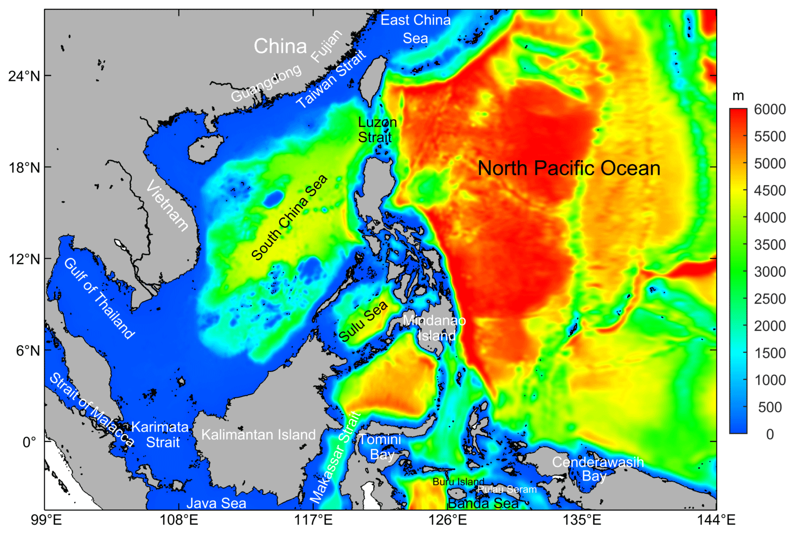
Figure 1 The model domain and bathymetry of SCSOFSv2.

First, we redistributed the land–sea grid mask layout to enable the systems mesh land boundary to fit the actual coastline better (Fig. 1). Based on a comparison with Fig. 1 in Zhu et al. (2016), a few areas have been changed from land to sea or vice versa, e.g., along the coast of the Chinese mainland, around Vietnam and the Gulf of Thailand, and around the coasts of Kalimantan Island and Mindanao Island. In addition, the Strait of Malacca had been opened to connect with the Karimata Strait, and the western lateral boundary was treated as an open boundary across the Strait of Malacca along 99^∘ E, instead of as a closed boundary in SCSOFSv1. Along the south lateral open boundary, the Java Sea was connected to the Makassar Strait to the southeast of Kalimantan Island and the Banda Sea was connected across the southern part of Buru Island and Pulau Seram, including Tomini Bay and the Cenderawasih Bay. It is obvious that the changes in the land–sea masks generated significant effects on the volume of sea water transportation in the model domain, and thus it contributes to the better simulation of the ocean circulations.

The bathymetry ETOPO1 dataset used in SCSOFSv1, which has a 1 arcmin grid resolution and is from the U.S. National Geophysical Data Center, was replaced by the General Bathymetric Chart of the Oceans (GEBCO_2014 Grid) global continuous terrain model for ocean and land, which has a 30 arcsec spatial resolution in SCSOFSv2. It was also merged with the measured topographic data in the coastal areas along the Chinese mainland and was adjusted with the tidal range. Following this, it was smoothed by applying a selective filter eight times to reduce the isolated seamounts on the deep ocean, and thus the “slope parameter” $r=\mathrm{\Delta }h/\mathrm{2}$ h is lower than the maximum value r₀=0.2 for each grid (Beckmann and Haidvogel, 1993; Marchesiello et al., 2009) in order to suppress the computational errors of the pressure gradient (Shchepetkin and McWilliams, 2003). Following this, the two grid stiffness ratios parameters, i.e., the slope parameter (r) and the Haney number, were changed from 0.22 and 9.78 in SCSOFSv1 to 0.17 and 13.80 in SCSOFSv2, respectively. The maximum depth was still set to 6000 m, but the minimum depth was changed from 10 m in SCSOFSv1 to 5 m in SCSOFSv2 (Wang, 1996). The final smoothed bathymetry is shown in Fig. 1.

For the vertical terrain-following coordinate, it was increased from 36 s-coordinate layers in SCSOFSv1 to 50 layers in SCSOFSv2. The transformation equation of the original formulation was also changed to an improved solution (Shchepetkin and McWilliams, 2005). The original vertical stretching function (Song and Haidvogel, 1994) was replaced with an improved double stretching function (Shchepetkin and McWilliams, 2005) to make it preserve a sufficient resolution in the upper 300 m in order to resolve the thermocline well. In this case, the thinnest layer was changed from 0.16 m in SCSOFSv1 to 0.09 m in SCSOFSv2 near the surface.

The new initial temperature and salinity fields in SCSOFSv2 were extracted from the Generalized Digital Environmental Model version 3.0 (GDEMv3, Carnes, 2009) global climatology monthly mean in January, which replaced version 2.2.4 of the Simple Ocean Data Assimilation (SODA, Carton and Giese, 2008) datasets. All four lateral boundaries are open, and the temperature, salinity, velocity, and elevation are obtained via spatial interpolation of the new SODA 3.3.1 datasets for the running 2005–2015 and SODA 3.3.2 datasets for the running 2016–2018 (Carton et al., 2018), instead of the original SODA 2.2.4. In the current version, the SODA 3.3.1 and 3.3.2 monthly mean ocean state variables are used, which are mapped onto the regular $\mathrm{1}/\mathrm{2}\times \mathrm{1}/\mathrm{2}{}^{\circ }$ Mercator horizontal grid from the original approximately $\mathrm{1}/\mathrm{4}\times \mathrm{1}/\mathrm{4}{}^{\circ }$ displaced pole non-Mercator horizontal grid at 50 vertical levels (z).

For the surface atmospheric forcing, we replaced the dataset from the NCEP Reanalysis 2 provided by the NOAA/OAR/ESRL PSL, Boulder, Colorado, USA, which is accessible from their website at https://psl.noaa.gov/data/gridded/data.ncep.reanalysis2.html (last access: 28 January 2022) (Kanamitsu et al., 2002), with the 6-hourly Climate Forecast System Reanalysis (CFSR, Saha et al., 2010a) for 2005–2011 and the Climate Forecast System version 2 (CFSv2, Saha et al., 2014) for 2011–2018. Both are archived at the National Centre for Atmospheric Research, Computational and Information Systems Laboratory, Boulder, Colorado. Its 0.2–0.3^∘ horizontal grid is significantly higher than the $\mathrm{2.5}\times \mathrm{2.5}{}^{\circ }$ resolution of the NCEP Reanalysis 2.

The net surface heat flux correction still follows the method of Barnier et al. (1995) in SCSOFSv2, but the parameter d$Q/$dSST, i.e., the kinematic surface net heat flux sensitivity to sea surface temperature (SST), is calculated using the SST, sea surface atmospheric temperature, atmospheric density, wind speed, and sea level specific humidity, instead of setting a constant number of −30 W m² K⁻¹ for the entire domain as in SCSOFSv1. Therefore, the parameter d$Q/$dSST varies temporally and spatially. In addition, infrared Advanced Very High Resolution Radiometer (AVHRR) satellite data are used in SCSOFSv2, which is an analysis constructed by combining observations from different platforms on a regular grid via optimum interpolation and is provided by the National Centres for Environmental Information, instead of the merged satellite's infrared and microwave sensor and the in situ (buoy and ship) global daily SST (MGDSST) data obtained from the Office of Marine Prediction of the Japan Meteorological Agency used in the SCSOFSv1.

The North Equatorial Current (NEC) is an interior Sverdrup steady current in the subtropical North Pacific and is located at 10–20^∘ N. It usually bifurcates into two branches after encountering the western boundary along the Philippine coast to the west of 130^∘ E (Qiu and Chen, 2010). However, the NEC is separated into two branches in the SCSOFSv1 due to the model's eastern lateral boundary setting. Its main branch is located at 9.5–13^∘ N, and the other branch is located at 14.5–17^∘ N (Fig. 2a), which is clearly not in line with the actual locations. The cause of the above result is that Guam (red circle in Fig. 2, located at about $\mathrm{13}{}^{\circ }{\mathrm{26}}^{\prime }$ N, $\mathrm{144}{}^{\circ }{\mathrm{43}}^{\prime }$ E) is included in SCSOFSv1, and its location is too close to the eastern lateral boundary. There is a sudden change in the bathymetry from over 3500 to below 500 m, serving as a large blockade to the NEC that once flowed into the model domain from the eastern lateral boundary. To resolve this problem in SCSOFSv2, the eastern lateral boundary was moved westward from 145 to 144^∘ E to narrow the model domain and exclude Guam. It was found that in SCSOFSv2, the simulated NEC remains as a single main current until 130^∘ E and then bifurcates into the southward-flowing Mindanao Current and the northward-flowing Kuroshio (Fig. 2b). In addition, it has been shown that the Kuroshio current of the eastern Philippines and the ocean circulations in the northeastern SCS grew stronger when Guam was removed. This indicates that the location of the lateral open boundary is very important to the results of the model simulation and that the results are better when it is set far enough away from the island, especially for islands located in the major ocean circulations.

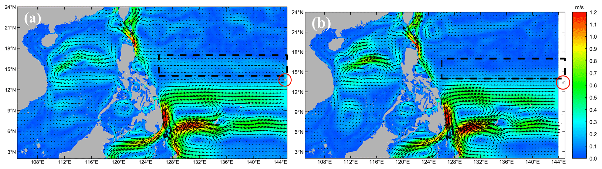
Figure 2 The multi-year monthly mean sea surface currents (the color shading indicates the current speed (m s⁻¹), and the arrows denote the current direction) with vertical averages of >100 m in May. Panel (a) is from SCSOFSv1, with the model domain including Guam, and panel (b) is from SCSOFSv2, with the eastern lateral boundary moved 1^∘ westward.

For the advection schemes of the momentum, third-order upstream and fourth-order centered schemes were used in both the horizontal and vertical directions. A harmonic mixing scheme was used for both the viscosity for momentum and the diffusion for tracers in the horizontal. The Mellor–Yamada Level 2.5 vertical turbulent mixing closure scheme was used for both the momentum and tracers. In SCSOFSv2, they are all set the same as in SCSOFSv1. Table 1 summarizes the main differences between SCSOFSv1 and SCSOFSv2 after upgrading.

Table 1 The main differences between SCSOFSv1 and SCSOFSv2.

The SCSOFSv2 is run using a 5 s time step for the external mode and a 150 s time step for the internal mode under all of the new configurations described above and those that will be introduced in Sect. 3. The reason for the modification of the time step is related to the change in the discrete schemes, which will be illustrated further in Sect. 3. First, a 26-year climatology run is conducted for spinning up the model, followed by a hindcast run from 2005 to 2018. The daily mean of the model results is archived and used for the subsequent evaluation.

3 Highlights, sensitive updates, and their impacts

Most of the bias and errors in the operational systems are mainly induced by several some major recurring problems, for example, external forcing, the intrinsic deficiencies of the numerical model (e.g., discrete schemes and sub-grid scale parameterization schemes), initial errors, and the assimilation schemes. In this section, we elaborate upon the solutions to such problems that are applied in SCSOFSv2 that were not discussed in Sect. 2. All of these solutions have significantly improved the model skill of the SCSOFS from different aspects, such as the SST, the three-dimensional temperature and salinity structures, and the comprehensive simulation skill, especially for the mesoscale processes.

3.1 Sea surface atmospheric forcing

Air–sea interactions are one of the most essential physical processes that affect the vertical mixing and thermal structure of the upper ocean. The air–sea fluxes mainly include the momentum flux, freshwater flux, and heat flux. The SST is an important indicator of the ocean circulation, ocean front, upwelling, and seawater mixing, and its variations mainly depend on the air–sea interactions and the ocean's thermal and dynamic factors (Bao et al., 2002). Thus, for the OOFS and ocean numerical modeling, the SST simulation and forecasting accuracy is an important metric for evaluating the modeling and forecasting performance.

The accurate input of the sea surface atmospheric forcing plays a key role in the performance of the model simulation of the SST. The ROMS provides two methods of introducing the sea surface atmospheric forcing: one is directly forcing the ocean model by providing momentum fluxes (wind stress), net freshwater fluxes, net heat fluxes, and shortwave radiation fluxes from the atmospheric datasets, and the other is employing the COARE3.0 bulk algorithm (Fairall et al., 2003) to calculate the air–sea momentum, freshwater, and heat turbulent fluxes using the set of atmospheric variables from the atmospheric datasets, including the wind speed at 10 m above the sea surface, the mean sea level air pressure, the air temperature at 2 m above the sea surface, the air relative humidity at 2 m above the sea surface, the downward longwave radiation flux, the precipitation rate, and the shortwave radiation fluxes (Large and Yeager, 2009). The calculations of the air–sea fluxes, sensible heat flux, latent heat flux, and longwave radiation can be referenced to Li et al. (2021). Since the SST used in the calculation of these three air–sea fluxes is extracted from the ocean model, an increase in the SST induces their variations in these fluxes, which then leads to increased loss of ocean heat and inhibits further increases in the SST and vice versa. Thus, an implicit SST-restoring effect can be formed between the SST and the SST-related air–sea heat fluxes. In this case, it is much easier to maintain the simulated SST at a reasonable level. The first method is employed in SCSOFSv1, and the second method, i.e., the bulk algorithm, is employed in SCSOFSv2.

In order to evaluate the performances of the different sea surface atmospheric forcing methods, we conducted a special experiment by changing the method based on SCSOFSv1, which is referred to as BulkFormula experiment in this paper. In this experiment, we used the merged satellite SST analysis with a multi-scale optimal interpolation, called the Operational SST and Sea Ice Analysis (OSTIA) system, with global coverage on a daily basis and a horizontal grid resolution of $\mathrm{1}/\mathrm{20}{}^{\circ }$ (∼6 km), which is produced by the Met Office (Donlon et al., 2012), to verify the results of the SCSOFS.

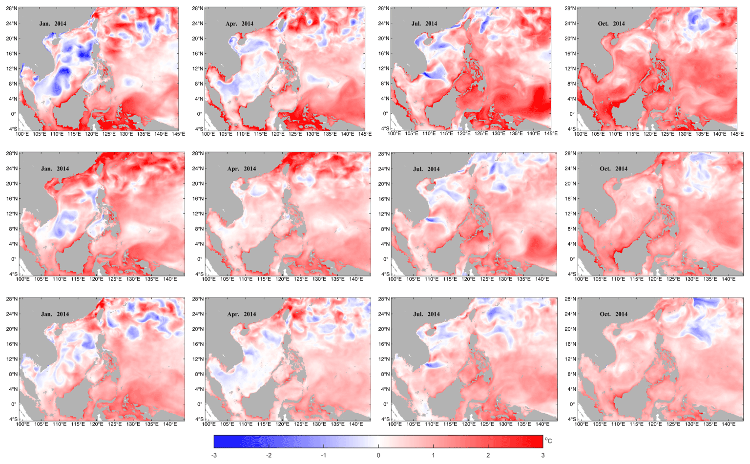
Figure 3 The monthly mean SST differences in January, April, July, and October of 2014: SCSOFSv1 minus OSTIA (upper row), BulkFormula minus OSTIA (middle row), and SCSOFSv2 minus OSTIA (lower row).

Figure 3 shows the distributions of the monthly mean SST differences in January, April, July, and October of 2014, which represent winter, spring, summer, and autumn, respectively. The SST differences were calculated using SCSOFSv1, BulkFormula, and SCSOFSv2 minus the OSTIA. It was found that the simulated SST were higher than the OSTIA in all three sets of results. The difference from SCSOFSv1 is significantly higher than the differences from the BulkFormula and SCSOFSv2. The maximum differences mainly occur near the coast (upper row of Fig. 3), especially for a few bays embedded in the mainland, which are nearly impossible to resolve well using two to three horizontal grids with a $\mathrm{1}/\mathrm{30}{}^{\circ }$ resolution and with very shallow water depth in SCSOFSv1. This is because the sea surface atmospheric forcing data are not accurate enough near the coast, and they provide an abnormally high amount of heat to the ocean, resulting in continuous heating of the coastal water. Thus, the simulated SST is beyond the normal level in SCSOFSv1. This phenomenon can be significantly alleviated by introducing the implicit SST-restoring effect using the COARE3.0 bulk algorithm, which is employed in both the BulkFormula and SCSOFSv2 (middle and lower rows of Fig. 3).

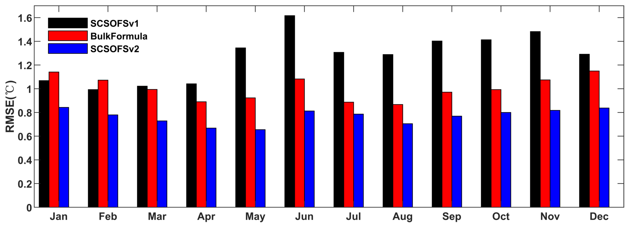
Figure 4 Domain-averaged monthly mean SST RMSE comparison of the SCSOFSv1 (black), BulkFormula (red), and SCSOFSv2 (blue) with the OSTIA SST in January, April, July, and October of 2014.

Figure 4 shows the bars of the domain-averaged root-mean-square error (RMSE) of the monthly mean SST differences between SCSOFSv1, BulkFormula, and SCSOFSv2 with respect to the OSTIA datasets for each month in 2014. It was found that the domain-averaged RMSE of the monthly mean SST differences for SCSOFSv1 is 0.99–1.62 ^∘C and that the annual mean value is about 1.27 ^∘C. The highest value (1.62 ^∘C) is in June, and the lowest value (0.99 ^∘C) is in February. The monthly mean RMSE for the BulkFormula run is 0.87–1.15 ^∘C, and the annual mean value is about 1.00 ^∘C. The maximum value (1.15 ^∘C) is in January and December, and the minimum value (0.87 ^∘C) is in August. The performance of the model's skill for the annual mean SST RMSE is improved by about 21 % by changing the sea surface atmospheric forcing method from direct forcing to the COARE3.0 bulk algorithm due to the implicit SST-restoring effect.

However, the domain-averaged RMSE of the monthly mean SST differences for the SCSOFSv1 is lower than that for the BulkFormula in January and February, especially in the shallow region around Taiwan. This indicates that the COARE3.0 bulk algorithm is not necessarily a panacea, even with an implicit SST-restoring effect. This may be dependent on the surface forcing data, and the use of an accurate dataset for the sea surface atmospheric forcing is more important than the selection of the forcing method (Li et al., 2019). It also may suffer from the complicated air–sea interactions and tidal mixing missing in the model.

3.2 Discrete tracer advection term schemes

Spurious diapycnal mixing is one of the traditional errors in state-of-the-art atmospheric and oceanic models, especially for regional terrain-following coordinate models, including those for both the continental slope and deep ocean (Marchesiello et al., 2009; Naughten et al., 2017; Barnier et al., 1998). Marchesiello et al. (2009) identified the problem as the erosion of the salinity from the southwestern Pacific model with steep reef slopes and distinct intermediate water masses based on the ROMS. They found that the ROMS cannot preserve the large-scale water masses while using the third-order upstream advection scheme during the spin-up phase of the model, and they proposed a rotated split upstream third-order scheme to decrease the dispersion and diffusion by splitting the diffusion from the advection. They implemented the rotated split upstream third-order scheme by employing a rotated biharmonic diffusion scheme with flow-dependent hyper diffusivity, satisfying the Péclet constraint.

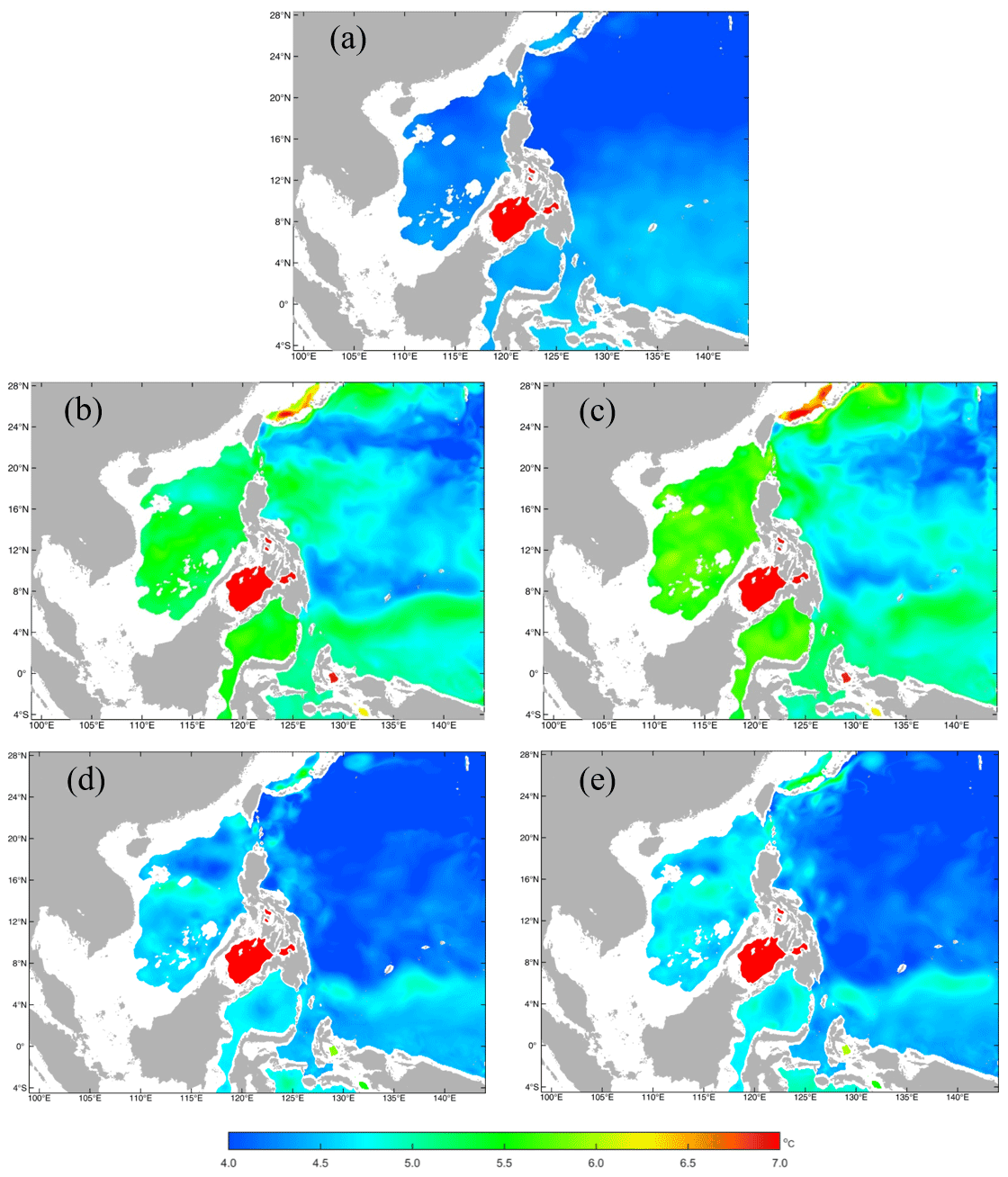
Figure 5 The distributions of the monthly mean temperature in the 1000 m layer in January from the (a) GDEMv3 climatology, (b) the 5th and (c) the 11th model year using the scheme combination of the UCI based on SCSOFSv1 for other model settings, and (d) the 5th and (e) the 11th model year using the scheme combination of the AAG based on SCSOFSv2 for other model settings.

For SCSOFSv1, a third-order upstream horizontal advection scheme, a fourth-order centered vertical advection scheme, and a scheme of horizontal mixing on EPI neutral (constant density) surfaces for tracers were selected (Shchepetkin and McWilliams, 2005). We encountered the same problem with the method of Marchesiello et al. (2009) regarding the temperature (Fig. 5b and c) and salinity (Fig. 6b and c) in the deep layer. Figure 5 and 6 show the distributions of the monthly mean temperature and salinity in the 1000 m layer in January from the GDEMv3 climatological initial fields, as well as the simulated results from the 5th and the 11th model years by using (i) the scheme combinations of the third-order upstream horizontal advection, fourth-order centered vertical advection, and horizontal mixing on EPI neutral surfaces (hereafter referred to as UCI) and (ii) the combination of the fourth-order Akima scheme (Shchepetkin and McWilliams, 2005) for both the horizontal and vertical advection terms and the scheme of horizontal mixing along geopotential surfaces (constant z) for tracers (hereafter referred to as AAG), respectively. The other settings are identical to those of SCSOFSv2. Figure 7 shows the comparisons of the time series of the domain-averaged monthly mean temperature and the salinity in the 1000 m layer simulated using the scheme combinations of the UCI in SCSOFSv1 and the AAG in SCSOFSv2. In order to lower computation costs, we only ran the model with the scheme combination of the UCI over 16 years until it reached a stable state.

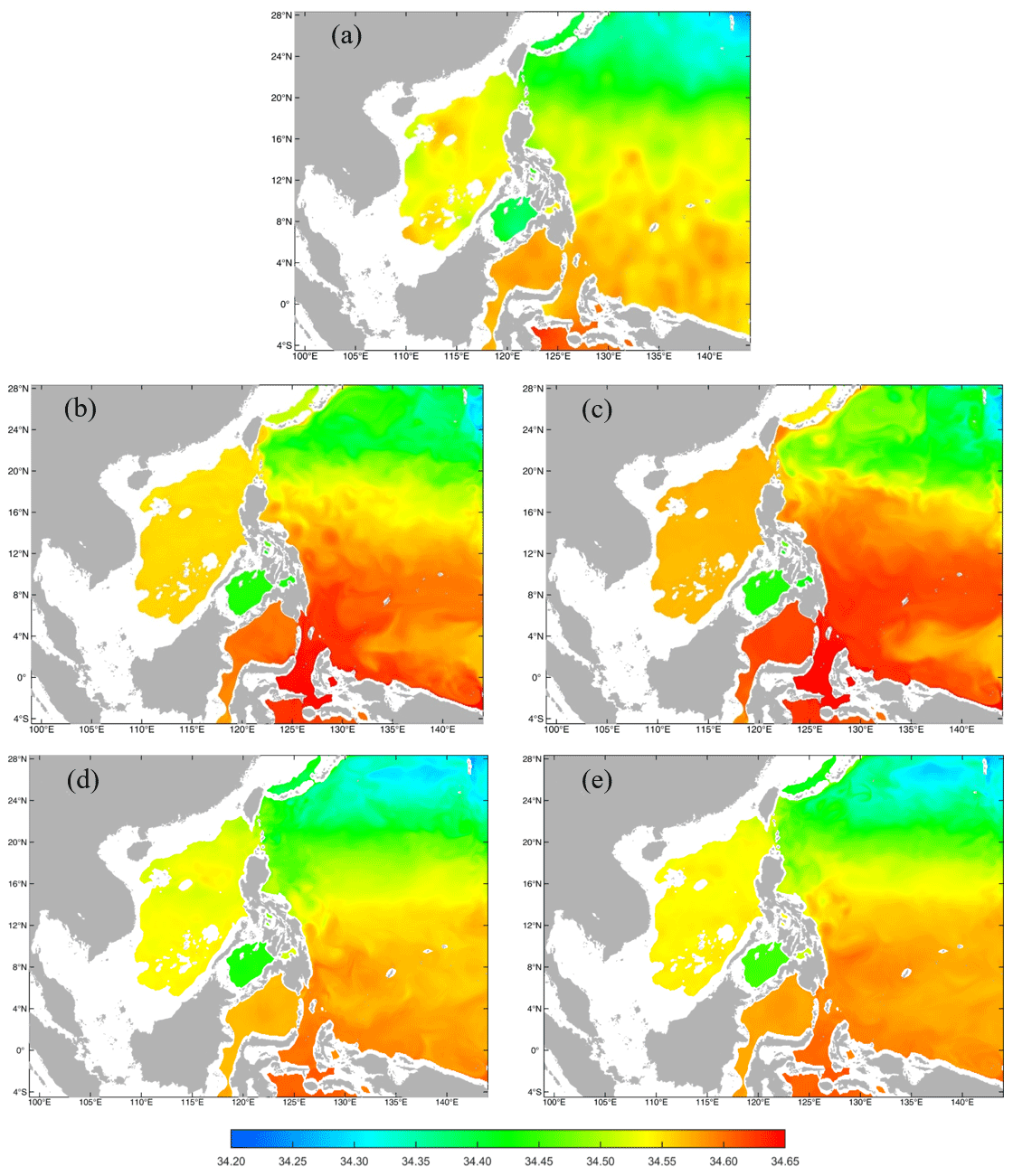
Figure 6 The same as Fig. 5 but for salinity.

The fourth-order Akima scheme is a little different from the fourth-order centered scheme because it replaces the simple mid-point average with harmonic averaging in the calculation of the curvature term. Since the time stepping is done independently of the spatial discretization in the ROMS, the Akima scheme has the advantage of reducing the spurious oscillations that arise from the non-smoothed advected fields with respect to the fourth-order centered scheme (Shchepetkin and McWilliams, 2003, 2005).

During the spin-up phase of the model from the initial conditions derived from GDEMv3, the temperature at 1000 m increases from the initial settings of 3.0–12.0 ^∘C (Fig. 5a) to 3.0–17.2 ^∘C (Fig. 5b), and the domain-averaged monthly mean value quickly increases from 4.4 to 5.1 ^∘C (Fig. 7a) in January of the fifth model year. The salinity at 1000 m increases from the initial settings of 34.26–34.62 (Fig. 6a) to 34.27–34.68 (Fig. 6b), and the domain-averaged monthly mean value increases rapidly from 34.50 to 34.54 (Fig. 7b) in January of the fifth model year. In particular, the increase in the domain-averaged monthly mean value is almost linear for both the temperature and salinity in the first 50 months, indicating a fast rate of increase and strong spurious diapycnal mixing (Fig. 7). These values are even higher in January in the 11th model year, the ranges (minimum and maximum values) reach 3.0–17.3 ^∘C and 34.26–34.73 for temperature (Fig. 5c) and salinity (Fig. 6c), respectively. The domain-averaged values are 5.3 ^∘C for temperature and 34.56 for salinity (Fig. 7). The areas with increasing temperature and salinity are mainly located on the steep slopes and nearby regions, e.g., the central basin of the SCS, the Sulawesi Sea, and the equatorial Pacific Ocean.

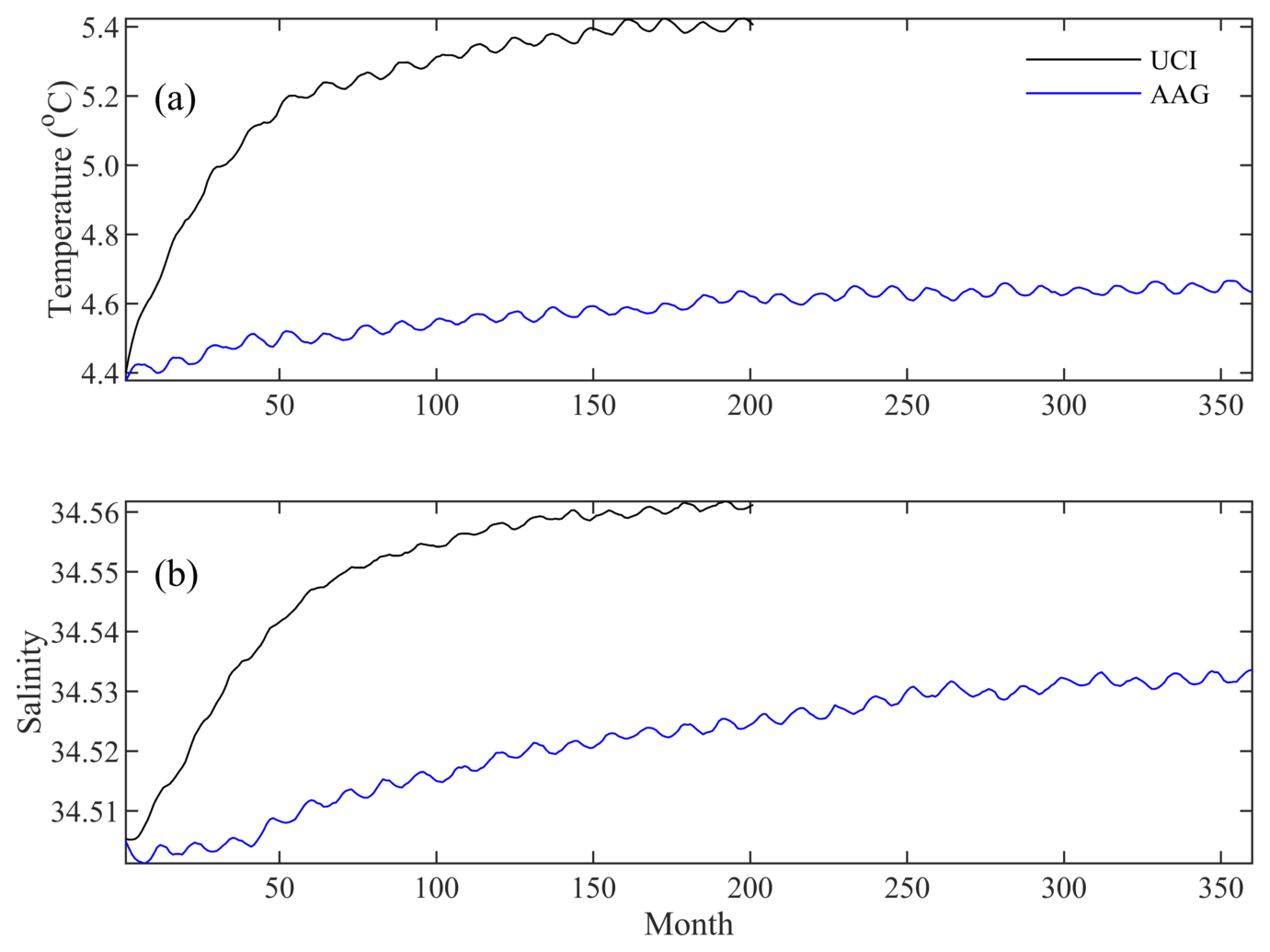
Figure 7 The time series of the domain-averaged monthly mean (a) temperature and (b) salinity in the 1000 m layer simulated using the scheme combinations of UCI (black line) and AAG (blue line).

To fix this problem, we tested various model settings and compiling options available in ROMS, such as increasing the number of vertical levels, changing the advection and diffusion schemes, horizontal mixing surfaces for tracers, and horizontal mixing schemes. The details of how the tested model settings effect on the spurious diapycnal mixing are beyond the scope of this paper, and they will be discussed in a separate paper.

The monthly mean temperature in the 1000 m layer from for SCSOFSv2 varies from the initial conditions of 3.0–12.0 ^∘C to 3.0–11.5 ^∘C (Fig. 5d), and the domain-averaged monthly mean value increases slightly from the initial value of 4.4 to 4.5 ^∘C in January in the fifth model year (Fig. 7a). The salinity at 1000 m varies from the initial conditions of 34.26–34.62 to 34.24–34.63 (Fig. 6d), and the domain-averaged monthly mean value only varies slightly from the initial value of 34.505 to 34.509 in January in the fifth model year (Fig. 7b). These values exhibit little variation until January of the 11th model year, the ranges are 3.0–11.3 ^∘C for temperature (Fig. 5e) and 34.25–34.63 for salinity (Fig. 6e), and the domain-averaged values are 4.6 ^∘C for temperature and 34.52 for salinity (Fig. 7). The increment of the domain-averaged value for temperature is about 0.2 ^∘C and that for salinity is about 0.03, but they remain stable after 20 model years (Fig. 7). This suggests that the spurious diapycnal mixing is significantly suppressed by the AAG scheme combination, which can preserve the characteristics of the water masses in the deep ocean well. In addition, the temperature and salinity biases in the subsurface layer are significantly improved, which will be shown in the latter part of this paper.

In addition, it was found that the model skill for the SST is also significantly improved using the new AAG scheme in SCSOFSv2 (Figs. 3 and 4). The maximum of the monthly mean differences between the SST simulated by SCSOFSv2 and OSTIA is about 3–4 ^∘C, which is obviously smaller than the results of the BulkFormula. Comparing with the results of SCSOFSv1 and BulkFormula, the results of SCSOFSv2 have a lower SST hot bias in the central Pacific Ocean relative to OSTIA, which is attributed to the new combination scheme. The domain-averaged RMSE of the monthly mean SST of SCSOFSv2 is 0.65–0.84 ^∘C, with an annual mean value of 0.77 ^∘C. The maximum value (0.84 ^∘C) is in January and December, and the minimum value (0.65 ^∘C) is in May. Compared with the results of the BulkFormula, the performance of the model skill based on the annual mean SST RMSE is improved by about 23 % due to the usage of the new combination scheme in SCSOFSv2. This indicates that the subsurface or deep-layer processes can affect the surface layer significantly due to vertical heat transport, which is induced by the barotropic and baroclinic instabilities that increase the eddy kinetic energy (Ding et al., 2021).

3.3 Data assimilation scheme

As was reported by Zhu et al. (2016), the original SCSOFSv1 used the multivariate Ensemble Optimal Interpolation (EnOI, Evensen, 2003; Oke et al., 2008) method to assimilate the along-track altimeter Sea Level Anomaly (SLA) data produced by SSALTO/DUACS and distributed by AVISO with support from the Centre National D'études Spatiales. During this upgrading process, we also improved several of the functions of the EnOI scheme and developed a new “Multi-source Ocean data Online Assimilation System” (MOOAS).

First, SCSOFSv1 only assimilated the along-track SLA data, while SCSOFSv2 is also able to simultaneously assimilate satellite AVHRR SST and in situ temperature and salinity vertical profile data from the Argo arrays. This is accomplished by combining the four variables' innovations (difference between the assimilated observation and the model forecast), background error covariances, and observation errors into each array. It is worth pointing out that the SLA data assimilated into the SCSOFS is a nearly real-time along-track L3 product for special assimilation, which is filtered but not subsampled, and that the dynamic atmospheric correction, ocean tide, long wavelength error correction are applied (CMEMS-SL-QUID-008-032-051, https://catalogue.marine.copernicus.eu/documents/QUID/CMEMS-SL-QUID-008-032-051.pdf, last access: 28 January 2022). The filtering processing consists of low-pass filtering with a cut-off wavelength of 65 km and a 20 d period using a Lanczos filter. The residual noise and small-scale signals are then removed via filtering. For the measurement errors of the SCSOFSv2, we set those of the SLA as constants of 3 cm according to the method of Taburet et al. (2018) and directly used the estimated error standard deviation of the analyzed AVHRR SST. For those of the Argo profiles, assuming they are a function of water depth (D) following Xie and Zhu (2010), ERR${}_T\left(D\right)=\mathrm{0.05}+\mathrm{0.45}\exp (-\mathrm{0.002}D)$ and ERR${}_S\left(D\right)=\mathrm{0.02}+\mathrm{0.10}\exp (-\mathrm{0.008}D)$.

Second, we introduced the method of computing the anomalies of the ensemble numbers used for constructing the background error covariance following Lellouche et al. (2013). In SCSOFSv1, the anomalies are computed by subtracting a 10-year average from long-term (typically 10 years) model free-run snapshots with a 5 d interval for the ocean state, i.e., the sea surface height and three-dimensional temperature, salinity, zonal velocity, and meridional velocity. In addition, the ensemble is selected within a 60 d window around the target assimilation date from each year, resulting in a total of about 130 members (Ji et al., 2015; Zhu et al., 2016). However, in SCSOFSv2, a Hanning low-pass filter is employed to create the running mean according to Lellouche et al. (2013) in order to obtain the intra-seasonal variability of the ocean state. Thus, the anomalies are computed by subtracting the running mean with a 20 d time window from the 10-year (2008–2017) free-run daily averaged results. In particular, it should be noted that the daily averaged free-run results are selected within a 60 d window, i.e., 30 d before and after the target assimilation date from each year in 2008–2017, and are used to compose the ensemble members, resulting in a total of about 590 members in SCSOFSv2. This means that the background error covariances rely on a fixed basis and an intra-seasonally variable ensemble of anomalies, which improves the dynamic dependency.

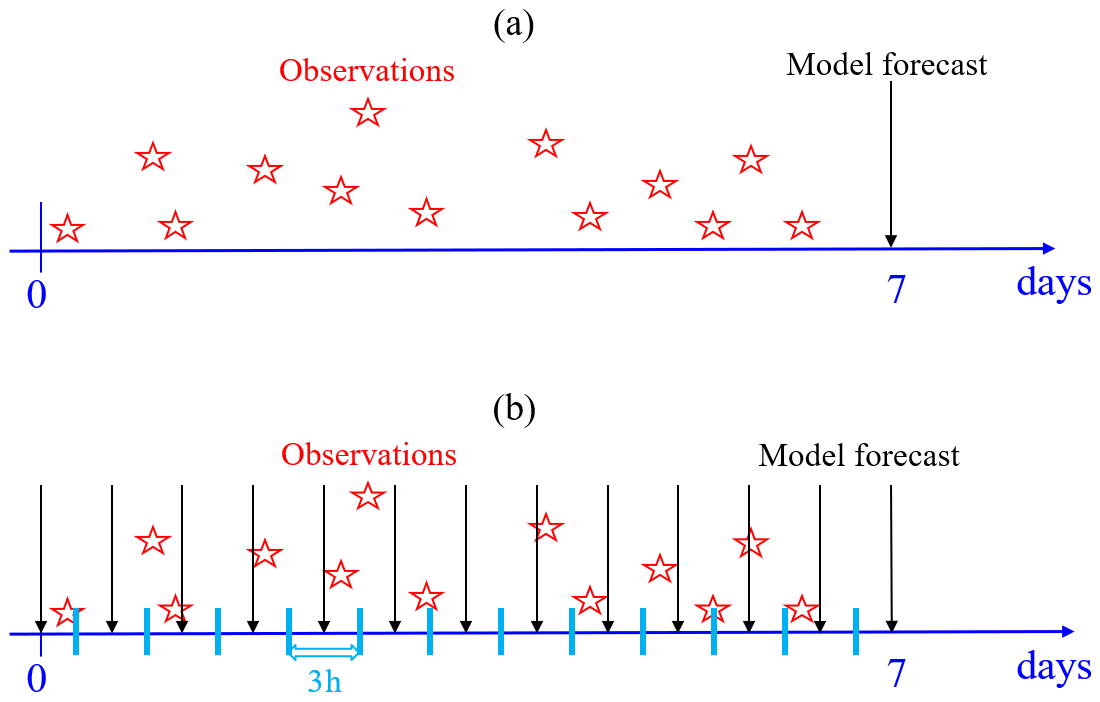
Figure 8 Schematic representation of the FGAT method: (a) not used in SCSOFSv1 and (b) used in SCSOFSv2. Red stars denote the observations, and the black arrows denote the archived snapshots of model forecast.

Third, for each analysis step with a 7 d assimilation cycle, all of the observations of the SLA within the 7 d time window before the analysis time are treated as being observed at the analysis time in SCSOFSv1, with the assumption that all of the observations are still valid at the analysis time. The time misfit between the observation and the model forecast causes non-negligible biases when calculating innovations. Actually, it is inconvenient to calculate all of the synchronous innovations between the observation and model forecast since the spatial and temporal distributions of the along-track SLA and Argo data are irregular and variable in each analysis step. In order to alleviate this deficiency, the First Guess at Appropriate Time (FGAT) method (Lee and Barker, 2005; Cummings, 2005; Lee et al., 2004; Sandery, 2018) was used in SCSOFSv2. Considering the intense computing and storage costs, we divided the 7 d time window into 56 total 3 h time slots (Fig. 8) and archived 57 snapshots with a 3 h interval, while the model forecast was run following the previous analysis run. Following this, the innovations were calculated within each 3 h time slot using the observations minus the nearest model forecast. This means that the maximum temporal misfit of the innovations between the observation and the model forecast were decreased from 7 d to 1.5 h by using FGAT. In addition, as in SCSOFSv1, the localization was still used with the radius set to 150 km.

In SCSOFSv1, the analysis increments of the sea surface height and three-dimensional temperature, the salinity, and the zonal and meridional velocities produced by each analysis of the data assimilation were applied to the model's initial fields at one time step. This inevitably induced a significant initial shock and spurious high-frequency oscillation in the model due to the imbalance between the increments and the model physics (Lellouche et al., 2013; Ourmières et al., 2006), and it usually resulted in rapid growth of the forecast error and even led to the model blowing-up after a few assimilation cycles or 1 or 2 years after the intermittent assimilation run. This was a threat to the stability and robustness of the OOFS. Therefore, we introduced the incremental analysis update (IAU) method (Bloom et al., 1996; Ourmières et al., 2006) to apply each analysis increment to the model integration as a forcing term in a gradual manner in SCSOFSv2 to diminish the negative impact. In this case, we obtained the tendency term by dividing the increments by the total number of time steps within an assimilation cycle, as in most IAU methodologies, in order to make sure the time integral of the tendency term equalled the analysis increment calculated by the EnOI.

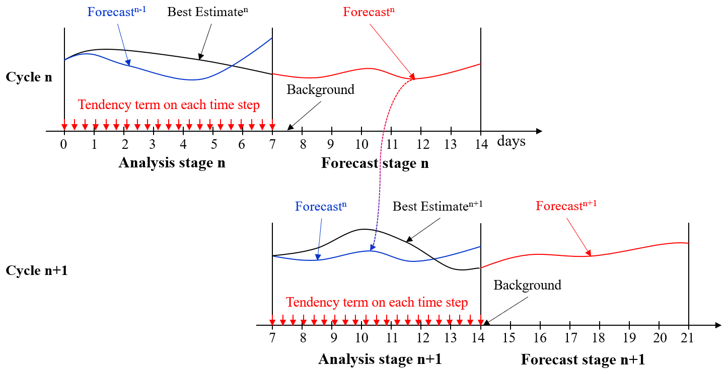
Figure 9 Schematic representation of the data assimilation procedure for two consecutive cycles, n and n+1, in SCSOFSv2 while considering the FGAT and IAU methods.

Once the FGAT and IAU methods were included in the EnOI scheme, the entire system's integral strategy had to be adjusted by adding one more model integration over the assimilation time window (Lellouche et al., 2013). In SCSOFSv1, only one time model integration is needed. This means that once the physical ocean model finishes a 7 d run (which does not need to archive snapshot fields) it outputs a restart field. The EnOI data assimilation module starts to calculate the analysis increments at the restart field time and adds it to the restart field. Following this, the physical ocean model implements a hot start from the updated restart field to run the 7 d of the next cycle.

However, in SCSOFSv2 model integration needs to be done two times due to the use of the FGAT and IAU methods (Fig. 8). This means that the physical ocean model needs to be integrated over 14 d in each assimilation cycle to add the tendency term to the model prognostic equations, due to the IAU method used during the first 7 d run (referred to as the analysis stage), to output a restart field at the end of seventh day for hot starting the ocean model in the next cycle and to output 3-hourly snapshot forecast fields during the second 7 d run (referred to as the forecast stage) to be used in the next cycle by the FGAT method. The model outputs from the analysis stage are referred to as the best estimate, and those from the forecast stage are referred as the forecast. The analysis increments are defined at halfway through the third day but not at the end of the seventh day as in SCSOFSv1. The observed SLA and Argo vertical profile data are within the 7 d time window, and the AVHRR SST data on the fourth day are used by the FGAT method.

4 Intercomparison and accuracy assessment

In order to demonstrate the improvements of the different SCSOFS sub-versions during the upgrading process, the results of the intercomparison and assessment are presented and discussed in this section using the GOV Intercomparison and Validation Task Team (IV-TT) Class 4 verification framework (Hernandez et al., 2009). Class 4 metrics were originally used for intercomparison and validation among different global or regional OOFSs or assimilation systems (Ryan et al., 2015; Hernandez et al., 2015; Divakaran et al., 2015). They include four metrics: the bias for assessing the consistency, the RMSE for assessing the quality or accuracy, the anomaly correlation for assessing the pattern of the variability, and the skill scores for assessing the utility of a forecast. They are calculated according to differences between the model values and the reference measurements in observations space for each variable over a given period and spatial domain. The physical variables used in the Class 4 metrics are the SST, SLA, Argo profiles, surface currents, and sea ice. The reference measurements, providing the ocean “truth”, are selected as follows: the SST data from the in situ drifting BUOY, the SLA data from the AVISO along-track data, and the temperature and salinity data from the Argo profiles. They are assembled by GOV IV-TT participating partners on a daily basis (Ryan et al., 2015).

Table 2 The major upgrades with respect to the previous version.

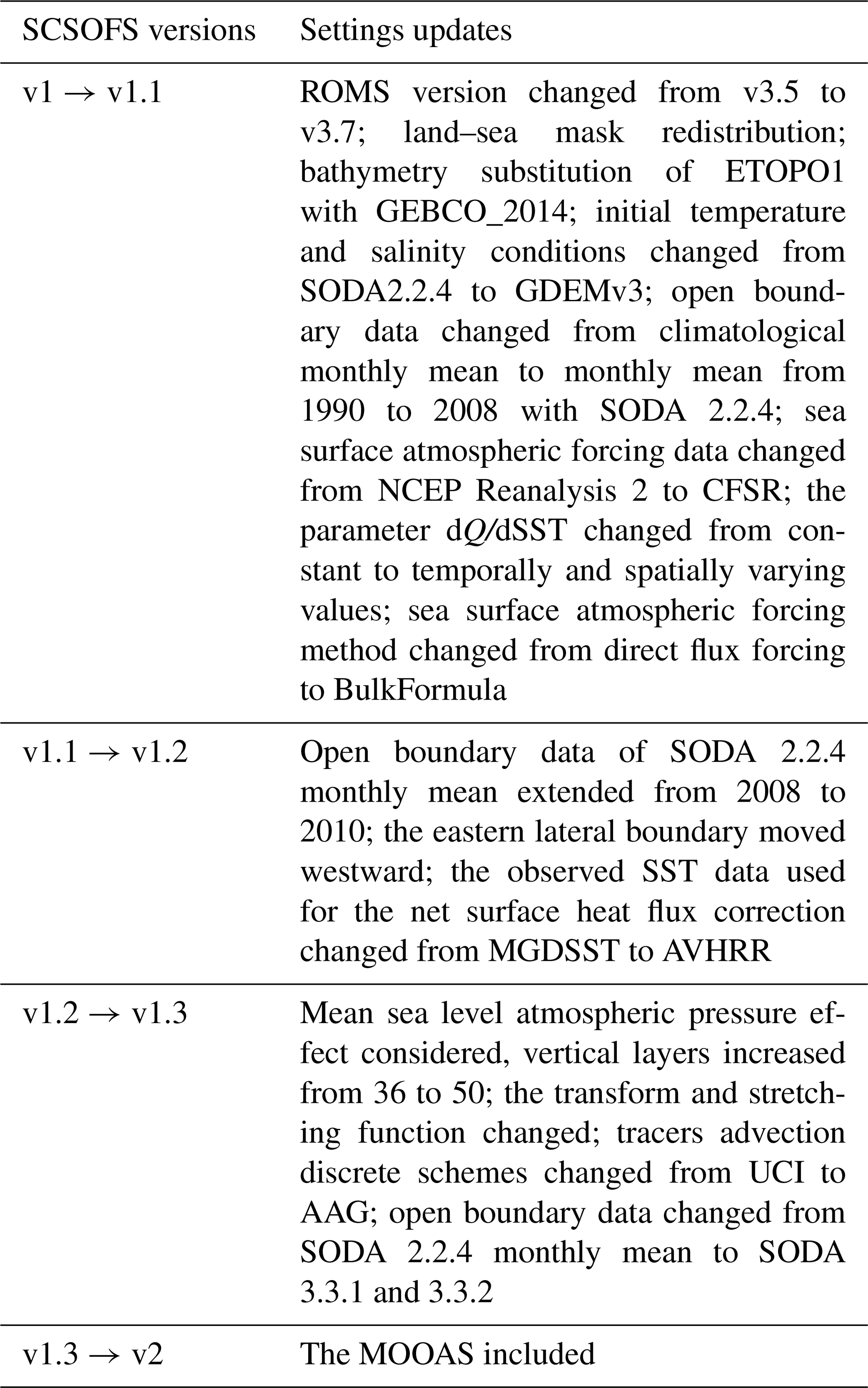
It is virtually impossible to exhaustively test and validate the performances of all of the upgrades described in Sects. 2 and 3. Here, we separate the entire upgrade procedure from SCSOFSv1 to SCSOFSv2 into four stages with three sub-versions (v1.1, v1.2, and v1.3) according to the reality. The major upgrades to each new version with respect to the previous version are listed in Table 2.

In this study, we used the Class 4 metrics and selected the first four physical variables (SST, SLA, and Argo profiles) to intercompare and assess the accuracies of the different sub-versions of the SCSOFS (Table 3). Since none of the reference measurement data described above have been used in these sub-versions of SCSOFS (except for SCSOFSv2) without data assimilation, they are reference observations that are independent from SCSOFS. The intercomparison and validation of the sub-versions without data assimilation were conducted for the model free-run results in 2013, and the intercomparison and validation between v1.3 and v2 were both conducted in 2018 to validate the performance of the MOOAS.

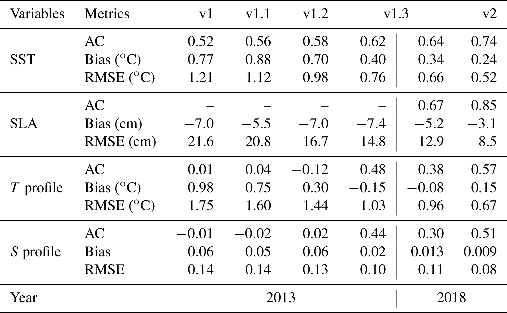
Table 3 Mean values of each metric of the four physical variables for the best estimates of each sub-version (T denotes temperature, S denotes salinity, AC denotes anomaly correlation).

4.1 SST

The accuracy of the SST continuously increased from version v1 to v2, and the anomaly correlation increased from 0.52 in v1 to 0.74 in v2, i.e., a 29.7 % improvement. The RMSE decreased from 1.21 ^∘C in v1 to 0.52 ^∘C in v2, i.e., a 57.0 % improvement, for the annual mean of the entire model domain-averaged in 2013 (or v1.3 and v2 in 2018) (Table 3). For versions v1, v1.1, v1.2, and v1.3, their anomaly correlation exhibited significant seasonal variations, with high anomaly correlations in summer and low anomaly correlations in winter. It was also found that the accuracy of the SST benefited from the sea surface atmospheric forcing method, as well as the usage of more accurate observed SST data for the sea surface heat flux correction, temperature advection discrete scheme, and SST data assimilation.

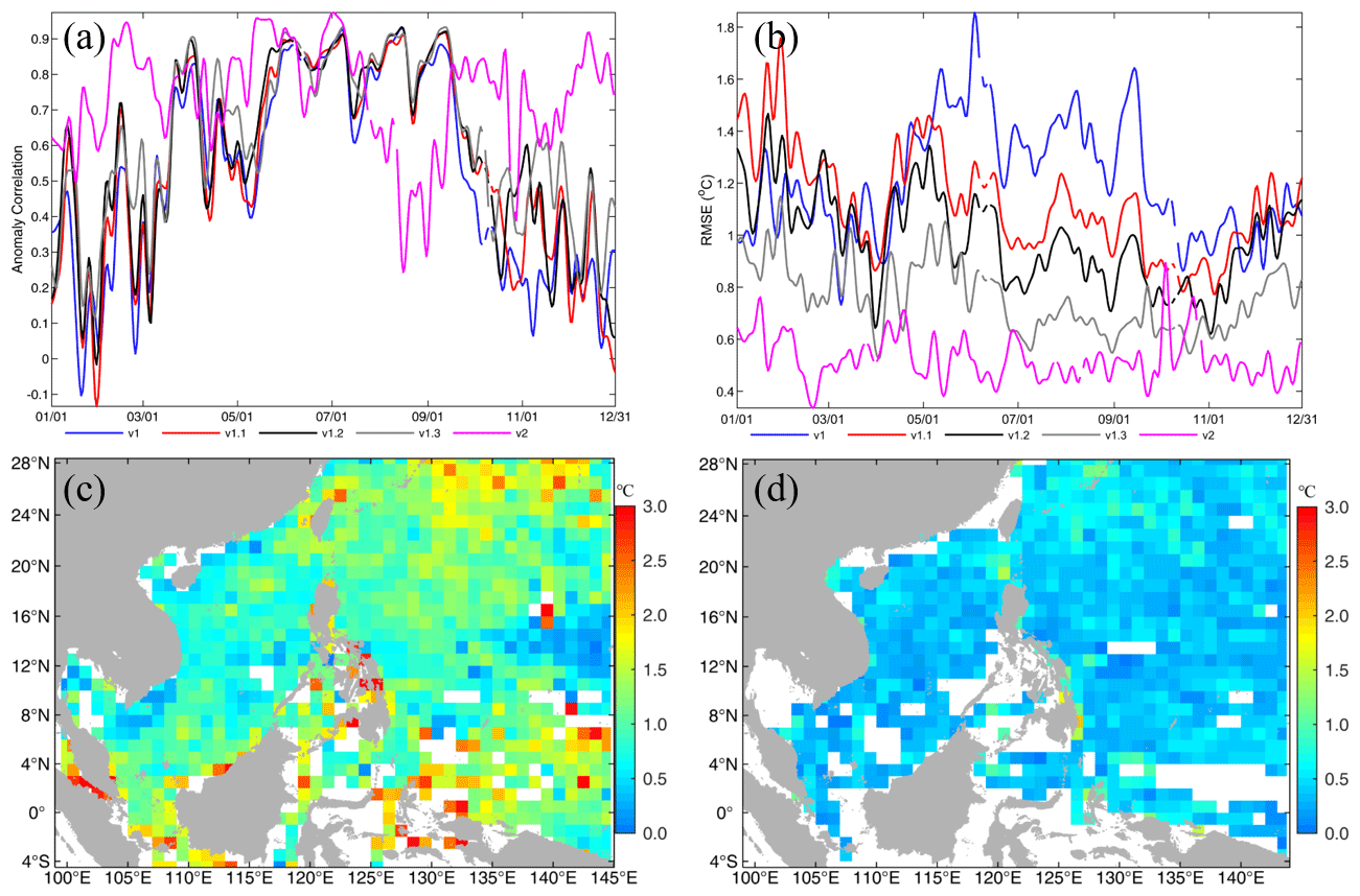
Figure 10 (a) Anomaly correlation and (b) RMSE time series of the SST best estimates for each version against observations as a function of time (7 d low-pass filter applied), i.e., v1, v1.1, v1.2, and v1.3 without data assimilation in 2013 and v2 with data assimilation in 2018. Horizontal distribution of the SST RMSE in a $\mathrm{1}\times {\mathrm{1}}^{\circ }$ bin for (c) v1 and (d) v2. The calculations were performed year-round in 2013 and 2018, respectively.

The improvement of the SST due to the sea surface atmospheric forcing method being changed mainly occurred in summer, exhibiting the same pattern as the results for 2014 in Figs. 3 and 4. However, using more accurate observed SST data for the sea surface heat flux correction improved accuracy of the SST simulation year-round (v1.2 in Fig. 10b). We also found that the OISST data were closer to the OSTIA than the MGDSST (figure not shown). Due to the benefits obtained from these changes, the maximum and minimum values of the SST RMSE have decreased from 1.92 and 0.71 ^∘C for v1 to 1.52 and 0.60 ^∘C for v1.2 for the entire year of 2013, respectively. It is worth mentioning that the AAG scheme combination not only improved the deep-layer temperature, but it also contributed to the improvement of the SST due to the internal baroclinic vertical heat transport. The maximum and minimum values of the SST RMSE were 1.21 and 0.52 ^∘C for v1.3. For the results with data assimilation in v2, the maximum and minimum values of the SST RMSE were only 1.13 and 0.32 ^∘C, respectively, which are better than the results for v1.3 year-round.

For the horizontal distribution of the SST RMSE, the large values were mainly located in the areas near the Equator, coastal areas, and the northern lateral boundary, with most of the values being larger than 1.5 ^∘C and a maximum value of about 6.67 ^∘C for v1 (Fig. 10c). For v1.3, due to the contributions of all of the above-described model updates, the pattern of the RMSE was similar to that of v1, i.e., basically without significant variations, but the maximum value decreased to 3.91 ^∘C, and most of the values were less than 1.2 ^∘C. After applying MOOAS in v2 (Fig. 10d), only a few large RMSE values were located on the eastern coast of the Philippines, with a maximum value of 2.09 ^∘C, and most of the values were lower than 0.8 ^∘C. This indicates that the performance of the SST in SCSOFSv2 was significantly improved by all of the updates described above.

4.2 SLA

For the entire upgrading process, the accuracy of the SLA also continuously increased from version v1 to v2, with the RMSE decreased from 21.6 cm for v1 to 8.5 cm for v2, i.e., a 60.6 % improvement, for the annual mean of the entire model domain-averaged in 2013 (or in 2018 for v1.3 and v2) (Table 3). Since there was an ongoing problem with the SLA climatology variable provided by GOV IV-TT during 2013–2015, we could not calculate the anomaly correlation for the SLA in 2013 and had to provide feedback on this issue to GOV IV-TT. However, based on the result of the SLA anomaly correlation in 2018, we found that it increased from 0.67 for v1.3 to 0.85 for v2, showing significant improvement in the correlation of the pattern of the variability between the model results and the climatology.

As can be seen from Fig. 11a, there was a slight decrease in RMSE for v1.1 with respect to v1, which mainly occurs in winter and rarely occurs in summer. This may be because there was no direct or intrinsic relationship between the model updates from v1 to v1.1 and the SLA in physics, and these updates mainly focused on the horizontal and temporal resolutions of the datasets. However, the improvement of the accuracy of the SLA in v1.2 with respect to v1.1 was significant, with the minimum and maximum of daily mean RMSE values decreasing from 0.12 and 0.31 cm for v1.1 to 0.11 and 0.23 cm for v1.2, respectively. Their annual mean value decreased from 20.8 cm for v1.1 to 16.7 cm for v1.2, i.e., a 19.7 % improvement. This may be the result of the well-represented NEC pattern due to the change in the model's eastern lateral boundary. With respect to v1.2, the accuracy of the SLA in v1.3 increased slightly, with an annual mean value of 14.8 cm and a 11.4 % improvement. This may be the result of the mean sea level air pressure correction and the modification of the temperature and salinity baroclinic structures due to the usage of the AAG. In addition, the most significant improvement in the SLA was introduced by the MOOAS, with minimum and maximum daily mean RMSE values of 6.1 and 12.1 cm for v2, respectively. The annual mean RMSE decreased to 8.5 cm, and the percentage increase reached 34.1 % with respect to v1.3 and to 60.6 % with respect to v1. This significant improvement was undoubtedly the result of the along-track SLA being assimilated into the system by the MOOAS.

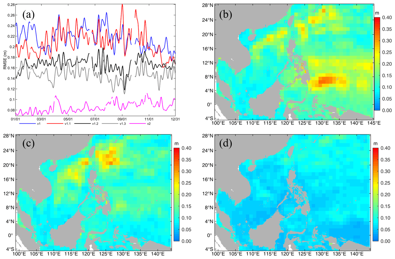
Figure 11 Panel (a) is similar to Fig. 10b but for the SLA. Panels (b–d) are similar to Fig. 10c and d but for the SLA of v1, v1.3 (in 2013), and v2, respectively.

For the horizontal distribution of the SLA RMSE, the large values of >20 cm were mainly located in the area of the NEC pathway, the continental shelf of the northeastern SCS, and to the northeast of the Luzon Strait, with a maximum value of 32.7 cm for v1 (Fig. 11b). For v1.3 (Fig. 11c), the large values in the area of the NEC pathway almost disappeared, the maximum RMSE was 30.3 cm, and most of the values were less than 20 cm, which can be interpreted as a better representation of the NEC pattern due to amendment of the model's eastern lateral boundary. In comparison to v1.3 or even v1, for v2, the SLA RMSE decreased dramatically for the entire model domain and did not contain areas with obvious large values. Its maximum value was only 18.2 cm, and most of the values were less than 10 cm. It is well known that abundant mesoscale eddies occur on both sides of the Luzon Strait, in the northeastern SCS, and in the western Pacific Ocean (Fig. 12a). The large SLA RMSEs in Fig. 11b and c indicate that a pure physical ocean model cannot capture these mesoscale processes well without assimilating SLA data (Fig. 12b). However, Fig. 11d shows a significant reduction in the SLA RMSE, indicating that the mesoscale eddies can be represented by SCSOFSv2 due to assimilation of the along-track SLA data, and the results are in good agreement with the satellite observations (Fig. 12c).

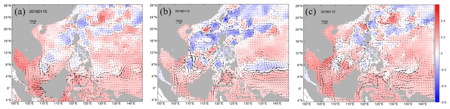
Figure 12 Daily averaged SLA (color shading) and surface velocity anomaly (vectors) on 15 January 2018 from AVISO, SCSOFSv1.3, and SCSOFSv2.

4.3 Temperature and salinity profiles

For the three-dimensional temperature and salinity distribution, by comparing the model results with the climatology temperature and salinity profiles, the results of first three versions exhibit poor correlations with the observations (Figs. 13a and 14a) and have large RMSEs (Figs. 13b and 14b), i.e., 1.44–1.75 ^∘C for temperature and 0.13–0.14 for salinity (Table 3), even though they decrease due to the model updates. In particular, for the vertical distribution, the RMSE can reach 3 ^∘C for temperature and 0.3 for salinity in the thermocline and halocline, respectively, and it remains larger than 1 ^∘C for temperature in the deep layer and 0.1 for salinity above a depth of 700 m (Figs. 13d and 14d). This may result from the spurious diapycnal mixing caused by the UCI combination scheme. The updates to v1.1 and v1.2 only slightly improved the three-dimensional temperature and salinity, and they did not contribute to their intrinsic improvement for either surface forcing or the lateral boundary conditions, with the exception of the surface layer with depths of less than 100 m.

However, once the AAG combination scheme was implemented in v1.3, the improvements to the three-dimensional temperature and salinity were significant with respect to the first three versions (Figs. 13a, b and 14a, b). The anomaly correlation increased to 0.38–0.48 for temperature and 0.30–0.44 for salinity, and the RMSE decreased to 0.96–1.03 ^∘C for temperature and 0.10–0.11 for salinity (Table 3). For the vertical distribution, the anomaly correlation remained at around 0.4 for both temperature and salinity in the entire water column, and it was greater than 0.6 for temperature in the surface layer (Figs. 13c and 14c). The RMSEs significantly decreased to less than 2 ^∘C for temperature in the thermocline, 0.25 for salinity in the halocline, and less than 1 ^∘C for temperature and 0.1 for salinity in the deep layer (Figs. 13d and 14d).

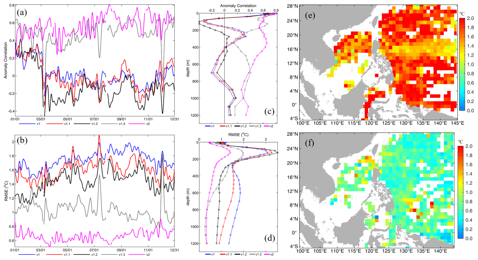
Figure 13 Panels (a) and (b) are similar to Fig. 10a and b but for the temperature profile. Panels (c) and (d) are vertical distributions of best estimates for each sub-version against observations as a function of depth, v1, v1.1, v1.2, and v1.3 without data assimilation in 2013 and v2 with data assimilation in 2018. Panels (e) and (f) are similar to Fig. 10c and d but for the temperature profile in v1 and v2, respectively.

For the horizontal distribution of the three-dimensional temperature and salinity RMSEs, the RMSE of the temperature was more likely to be >1.5 ^∘C with maximum and minimum values of 4.45 and 0.49 ^∘C (Fig. 13e), respectively, while the RMSE of salinity was greater than 0.1, with maximum and minimum values of 0.81 and 0.06 (Fig. 14e), respectively, for v1. The large values for salinity were mainly located in the SCS and near the Equator in the Pacific Ocean. The trend was the same as the time series of the RMSE. The horizontal distributions of the temperature and salinity RMSEs decreased slightly from version v1 to v1.2, but they dramatically decreased in v1.3 (figures not shown). Since it benefited from the usage of the AAG combination scheme in v1.3, most of the temperature RMSEs were lower than 1.0 ^∘C, with maximum and minimum values of 1.72 and 0.11 ^∘C, respectively, and most of the salinity RMSEs were less than 0.1, with maximum and minimum values of 0.62 and 0.03 in 2013, respectively.

By employing the MOOAS, the accuracies of the three-dimensional temperature and salinity were continuously improved in v2 compared to v1.3 for all of the metrics in 2018 (Figs. 13 and 14). The mean anomaly correlations increased from 0.38 to 0.57 for temperature and from 0.30 to 0.51 for salinity. The mean RMSEs decreased from 0.96 to 0.67 ^∘C for temperature, and from 0.11 to 0.08 for salinity (Table 3). For the vertical distributions of the anomaly correlation for temperature, it was >0.6 in the surface layer, was >0.4 above 600 m, and was >0.3 in the deep layer (Fig. 13c). The RMSE of the temperature was less than 1.5 ^∘C for the entire vertical profile, and similar to other versions the maximum value was located in the thermocline, but the error decreased dramatically (Fig. 13d). In contrast to temperature, the vertical anomaly correlation of the salinity did not significantly improve below 200 m in v2 with respect to v1.3, and it was only slightly higher than that of v1.3 (Fig. 14c) above 200 m. The salinity RMSE was less than 0.25 for the entire vertical profile, with the maximum value located at the surface and decreasing with depth and decreasing to less than 0.05 below 600 m (Fig. 14d).

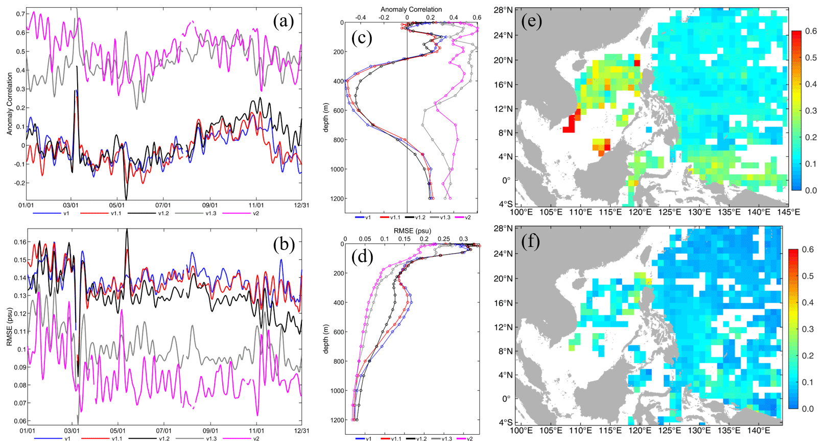
Figure 14 Similar to Fig. 13 but for salinity profile.

For the horizontal RMSE distribution of v2, most of the temperature RMSEs were greater than 0.8 ^∘C, with maximum and minimum values of 1.96 and 0.03 ^∘C (Fig. 13f), respectively, and most of the salinity RMSEs were greater than 0.1, with maximum and minimum values of 0.35 and 0.01, respectively, in 2018 (Fig. 14f).

5 Conclusions

The results of this study illustrate the major updates made to SCSOFSv1 in terms of physical model settings, inputs, and EnOI data assimilation scheme in the last few years, following the recommendations of Zhu et al. (2016), such as redistributions of the land–water grid mask; changes in the data sources of the bathymetry, the initial conditions, and the sea surface forcing method; changing the open boundary conditions to higher spatial and temporal resolutions; shifting the eastern lateral boundary westward; and increasing the vertical layers of the model.

The three most significant updates were highlighted in this paper. First, the sea surface atmospheric forcing method was changed from direct forcing to the BulkFormula to acquire an implicit SST-restoring effect for the air–sea interactions using the COARE3.0 bulk algorithm. The upgrades led to more reasonable SST simulations by eliminating abnormal values, significantly decreasing the maximum value of the monthly mean differences between the simulated SST and OSTIA and decreasing the domain-averaged RMSE of the monthly mean SST from 0.99–1.62 ^∘C in SCSOFSv1 to 0.87–1.15 ^∘C in the BulkFormula run. The annual mean value decreased from 1.27 to 1.00 ^∘C, indicating that the performance of model's skill improved by about 21 %.

Second, the AAG scheme was substituted for the tracers advection term discrete scheme UCI in order to suppress the spurious diapycnal mixing problem. After this substitution, the domain-averaged monthly mean temperature in the 1000 m layer decreased from 5.1 to 4.5 ^∘C, and the domain-averaged monthly mean salinity decreased from 34.54 to 34.509, in January of the fifth model year. Even after 20 model years, the domain-averaged values of the temperature and salinity increments were only about 0.2 ^∘C and 0.03, respectively, suggesting that the AAG combination scheme can preserve the characteristics of the water masses in the deep ocean well. In addition, the model skill for the SST also benefited from the AAG combination scheme, and the annual mean domain-averaged RMSE decreased from 1.00 to 0.77 ^∘C, i.e., a 23 % improvement in the performance.

Third, the original EnOI method in SCSOFSv1 was upgraded to the MOOAS by adding four new functions. The multi-source observation data (SST, SLA, and Argo profiles) were simultaneously assimilated. The Hanning high-pass filter was applied to the ensemble members from 10 years of free run while calculating the background error covariances to improve the dynamic dependency. The FGAT method with a 3 h time slot was used to calculate the innovations, and the IAU technique with a 7 d time window was used to analyze the increment in the model integration in a gradual manner.

Moreover, intercomparison and accuracy assessment of the five versions were conducted based on the GOV IV-TT Class 4 metrics for four physical variables, i.e., the SST, SLA, and Argo profiles. The improvement in the accuracy of the simulated SST was mainly due to the use of more accurate observed SST data for the sea surface heat flux correction, the use of the BulkFormula method for the sea surface atmospheric forcing, and the use of the AAG discrete temperature advection scheme. The improvement of the accuracy of the SLA as mainly due to the good representations of the NEC pattern obtained by modifying the model's eastern lateral boundary, the mean sea level air pressure correction, and the improvement of the three-dimensional temperature and salinity baroclinic structures by using the AAG scheme. The improvement of the three-dimensional temperature and salinity mainly benefited from the use of the AAG non-spurious diapycnal mixing combination scheme.

Finally, the remarkable improvements in all of the above four variables also benefited from use of the MOOAS. With respect to v1.3, for the v2 using the MOOAS, the domain-averaged annual mean SST RMSE decreased from 0.66 to 0.52 ^∘C, i.e., a 21.2 % improvement. The SLA RMSE decreased from 12.9 to 8.5 cm, i.e., a 34.1 % improvement. The temperature profile's RMSE decreased from 0.96 to 0.67 ^∘C, i.e., a 30.2 % improvement. The salinity profile's RMSE decreased from 0.11 to 0.08, i.e., a 27.3 % improvement.

Although SCSOFSv2 is greatly improved compared to the previous versions, some biases still exist, such as the structures of the temperature and salinity profiles in the subsurface, especially in the thermocline and halocline. We plan to continue to improve the system in terms of both the physical model settings and the data assimilation scheme in the next step, including a sub-grid parameterization scheme for the unresolved physical processes, a vertical turbulent mixing scheme to consider wave mixing, a more accurate input and forcing data source, and assimilation of more or new types of observations (glider or mooring three-dimensional temperature and salinity profiles, drifting buoys, in situ velocity data from moorings) into the system.