The E3SM Diagnostics Package (E3SM Diags v2.7): a Python-based diagnostics package for Earth system model evaluation

The E3SM Diagnostics Package (E3SM Diags) is a modern, Python-based Earth system model (ESM) evaluation tool (with Python module name e3sm_diags), developed to support the Department of Energy (DOE) Energy Exascale Earth System Model (E3SM). E3SM Diags provides a wide suite of tools for evaluating native E3SM output, as well as ESM data on regular latitude–longitude grids, including output from Coupled Model Intercomparison Project (CMIP) class models.

E3SM Diags is modeled after the National Center for Atmospheric Research (NCAR) Atmosphere Model Working Group (AMWG, 2022) diagnostics package. In its version 1 release, E3SM Diags included a set of core essential diagnostics to evaluate the mean physical climate from model simulations. As of version 2.7, more process-oriented and phenomenon-based evaluation diagnostics have been implemented, such as analysis of the quasi-biennial oscillation (QBO), the El Niño–Southern Oscillation (ENSO), streamflow, the diurnal cycle of precipitation, tropical cyclones, ozone and aerosol properties. An in situ dataset from DOE's Atmospheric Radiation Measurement (ARM) program has been integrated into the package for evaluating the representation of simulated cloud and precipitation processes.

This tool is designed with enough flexibility to allow for the addition of new observational datasets and new diagnostic algorithms. Additional features include customizable figures; streamlined installation, configuration and execution; and multiprocessing for fast computation. The package uses an up-to-date observational data repository maintained by its developers, where recent datasets are added to the repository as they become available. Finally, several applications for the E3SM Diags module were introduced to fit a diverse set of use cases from the scientific community.

1 Introduction

Earth system model (ESM) developers run automated analysis tools on candidate versions of models and rely on the metrics and diagnostics generated by those tools for key insights into model performance and to inform model development. Continued efforts from climate scientists and software engineers make these tools more efficient and comprehensive so that they may play an important role in providing condensed and credible information from aspects of climate systems and to support stakeholders and policymakers (Eyring et al., 2019).

Phillips et al. (2014)Eyring et al. (2016)Righi et al. (2020)Gleckler et al. (2008)Gleckler et al. (2016)Collier et al. (2018)Maloney et al. (2019)

Table 1 A summary of selected evaluation tools for components of Earth system models. The packages described are sorted roughly by first (publication) available year in ascending order. The main feature, primary programming language/installation, input requirement and references are summarized in the table. “CMIP-like” refers to netCDF input files compliant with CMIP specifications: i.e., one variable per file and mapped to regular spherical coordinates grids (CMIP6 Output Grid Guidance, https://docs.google.com/document/d/1kZw3KXvhRAJdBrXHhXo4f6PDl_NzrFre1UfWGHISPz4/edit, last access: 12 December 2022). User-facing documentation for each tool is available from the GitHub repository (repo) link for each tools.

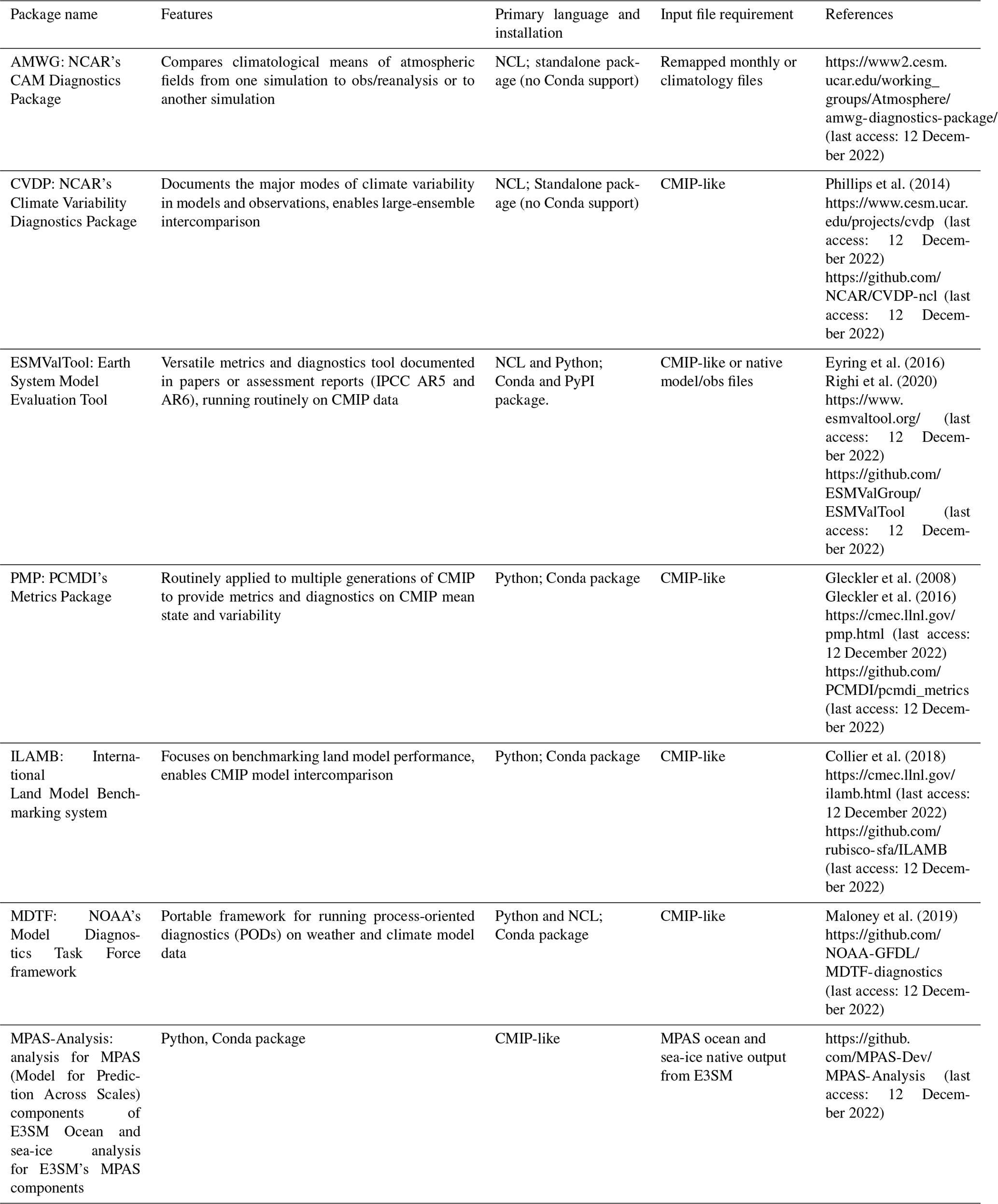
A number of established evaluation packages have been developed to facilitate analyzing ESMs and their atmosphere, land-surface, ocean and sea-ice component modules. Table 1 provides a list of some of the most widely used tools designed to evaluate different components of coupled Earth system models. Most tools listed here have started with a main focus on one ESM component but have evolved to analyze other ESM realms too, for example, the International Land Model Benchmarking (ILAMB) system, which specializes in land model components and includes functionality for evaluating ocean outputs (via International Ocean Model Benchmarking, IOMB); and the Earth System Model Evaluation Tool (ESMValTool) has a solid evaluation component for ocean model data in addition to its atmospheric component. The MPAS (Model for Prediction Across Scales)-Analysis tool has a focus on evaluation of the ocean and sea ice.

One of the most well established climate data evaluation packages, the Atmosphere Model Working Group diagnostics package (AMWG, 2022) was developed at the National Center for Atmospheric Research (NCAR) and has been used widely for the Community Atmosphere Model (CAM), the atmospheric component of the Community Earth System Model (CESM). This package was written in the NCAR Command Language (NCL), which cultivated a mature and extensive collection of libraries to support atmospheric data analysis and visualization. The same language is also used to script NCAR's Climate Variability Diagnostics Package (CVDP; Phillips et al., 2014), which focuses on evaluating modes of variability and facilitating model intercomparison. Both AMWG and early versions of CVDP were designed specifically for model output following CESM convention.

By formulating common data standards for ESM output and distributing these data broadly, the World Climate Research Programme (WCRP) Coupled Model Intercomparison Project (CMIP) initiative created a unique opportunity for generalizing and relaxing the input data requirement for evaluation packages and built a foundation for multi-model evaluation. A number of software packages, including the ESMValTool, the PCMDI Metrics Package (PMP) and ILAMB (see Table 1), were created with a goal to analyze data following CMIP conventions and evaluate data from the CMIP archive, served by the Earth System Grid Federation (ESGF). Among these tools, ESMValTool has been the primary package for production of figures for the Intergovernmental Panel on Climate Change (IPCC) assessment reports (Eyring et al., 2016; Righi et al., 2020). An outcome from these massive intercomparison efforts covering generations of CMIP models is that the community has been able to identify common biases present in ESMs, in turn motivating the development of more process-oriented metrics and diagnostics aimed at addressing those model deficiencies (Maloney et al., 2019). As more and more such analyses are being developed by individual scientists and agencies across the world, there is a growing technical challenge to synthesize analysis data and scripts generated and to make those analyses inter-operable. To address the need for consistent operation of several diagnostics from a single interface, ESMValTool has invested heavily in integrating evaluation tools directly into their software system. However, other groups have sought to avoid centralization of the development process. The National Oceanic and Atmospheric Administration (NOAA) Model Diagnostics Task Force (MDTF) framework has adopted a process-oriented diagnostics (PODs) concept where each POD aims to address several aspects of a particular Earth system process or phenomenon. POD contributors must follow common standards to be part of the MDTF. The US Department of Energy (DOE) Coordinated Model Evaluation Capabilities (CMEC) project takes a different approach, which is to bring existing established packages (PMP, ILAMB and others) into compliance with a set of common standards and provide a thin software layer (https://github.com/cmecmetrics/cmec-driver, last access: 12 December 2022) to make the packages inter-operable. MDTF and CMEC have worked in partnership to ensure compatibility of their standards and thus inter-operability of their diagnostics.

Scientifically oriented software packages are impacted by changes in programming languages and standard software development practices. Over recent decades, with growing support in Earth science, Python has become a leading programming language for analysis in the geosciences. Most recent efforts in ESM analysis packages heavily rely on Python and its open-source scientific ecosystem. Distribution of these Python packages is now mostly accomplished through Anaconda/Miniconda (https://docs.conda.io/en/latest/miniconda.html, last access: 12 December 2022). Similar library dependencies and distribution methods also increase opportunities for collaborative development of software packages, for instance by reuse of software modules and maintenance of a unified software environment.

This paper introduces a new Python package, E3SM Diags, which has been developed to support ESM development and has been used routinely in the model development of DOE's Energy Exascale Earth System Model (E3SM) (Leung et al., 2020). This effort was inspired by the AMWG diagnostics package, which is soon to be retired. Developers of E3SM Diags are committed to following modern software practices, in anticipation of a pivot within the model development community towards Python and its ecosystem of libraries for climate science research. A goal of this project is to create a central code repository to orchestrate analysis within the E3SM project and its ecosystem and to enable a pathway for community contributions to the model evaluation workflow. This paper is a comprehensive description of E3SM Diags and covers the current status of its development (as of version 2.7) and applications. A discussion on future work and outlook is also outlined.

2 Technical overview of E3SM Diags

E3SM Diags is open-source software developed and maintained on GitHub under the E3SM-Project (https://github.com/E3SM-Project/e3sm_diags, last access: 12 December 2022). It is a pure Python package and distributed through Conda via the conda-forge channel. This tool adopts Python's design and development practices, aiming to be modular, configurable and extendable. Dependencies of the package include many standard Python open-source scientific libraries: NumPy (Harris et al., 2020) for array manipulation, CDAT (including cdms2, cdtime, cdutil, genutil, cdp; Williams, 2014; Doutriaux et al., 2021) for climate data analysis, and Matplotlib with the Cartopy add-on (Met Office, 2010–2015) for visualization. Additional tools for netCDF data handling, including NCO (Zender, 2008, 2014), TempestRemap (Ullrich and Taylor, 2015; Ullrich et al., 2016) and TempestExtremes (Ullrich and Zarzycki, 2017; Ullrich et al., 2021), are used for pre-processing native E3SM and observation data.

Figure 1 A schematic overview of the E3SM Diags structure and workflow. The primary input includes the following components (blue boxes): the user configuration through setting up a Python run script or a command line, model data pre-processed from native E3SM history files, and reformatted observation data if needed to configure a model/observation comparison run. Helper scripts for data pre-processing are provided in the repo. The main E3SM Diags driver (green boxes) parses the user input and drives individual sub-drivers for specified diagnostics sets. The output (orange boxes) includes an HTML page linking to a provenance folder including run scripts and environment YAML files and each individual diagnostic set, which includes HTML pages, figures, tables, provenance and optional intermediate netCDF files.

Figure 1 depicts a schematic overview of the code structure and workflow. Running the package requires user configuration and both test and reference data as input. An E3SM Diags run performs climatology comparison between two datasets: a test model set and a reference set. The reference set could be another test model or observational dataset. In the most common use case, to compare an instance of model output to observational and reanalysis data, a copy of pre-processed observational and reanalysis data needs to be downloaded from the E3SM data server (see “Data availability” section for location). The user configuration includes basic parameters to specify input/output (I/O) paths, selected diagnostics sets, output format, and other options. These parameters can be passed either through a Python script (see examples in Appendix B and in E3SM Diags GitHub repo) or via a command line (see an example in Sect. 3.1). Between the two methods, configuring a Python script to use E3SM Diags (module name: e3sm_diags) via an API (application programming interface) is a more typical use to generate comprehensive diagnostics. The command line is useful for reproducing or refining figures when managing only a few figures or for particular parameters (e.g., variables or seasons). E3SM Diags can be run in either serial or multiprocessing mode (using Dask). Task parallelism is currently performed on one computer node. Running distributed tasks in parallel across computer nodes will be explored in future releases.

The E3SM Diags codebase is designed to be modular. Each diagnostic set is self-contained and composed of a driving script that includes the set-specific file I/O, computation, plotting, parameter set, parser set, viewer, and default configuration files that describe pre-defined default variables and plotting parameters. A script e3sm_diags_driver.py serves as a main driver to parse input parameters and drives each set. The output from each run, including figures, tables, provenance and links to optional intermediate files, is organized into HTML pages and made interactive through a browser. Shared among diagnostics sets are commonly utilized modules, including built-in functions to generate derived variables, to select diagnostics regions, to generate climatologies and so on.

The development effort follows standard software development practices. Continuous integration and continuous delivery/continuous deployment (CI/CD) workflows are managed through GitHub Actions. As of version 2.5, GitHub Actions workflows include automated quality assurance checks, unit and integration testing, and documentation generation.

Two types of test are included: unit tests are used to verify if small elements of code units give consistent results during development; integration tests allow for a systematic consistency check of all diagnostics incorporated; an image checker is built to verify changes in figures/metrics over source code and dependency version change. The documentation web page is built with Sphinx (Brandl, 2021). Source files to generate documentation are version-controlled and managed on a main branch.

In addition to the GitHub repository, E3SM Diags also includes a set of observational datasets which were processed from their original data source into time-series and/or climatology files to use as input for model validation. The Python and Shell scripts to process these data are available as part of the package provenance in the code repository.

E3SM Diags can be set up on a Linux or macOS system straightforwardly. A general guide to setting up and running E3SM Diags is provided in Appendix A. And a quick example of an experiment running this tool on a supercomputer at NERSC (the National Energy Research Scientific Computing Center) is described in Appendix B.

Figure 2 Latitude–longitude maps of annual-mean precipitation comparing a candidate version of E3SM with reference data from Global Precipitation Climatology Project (GPCP) v2.3, with test/model data in the upper plot (a), reference/observation data in the middle (b) and the difference (upper − middle) plot at the bottom (c). Metrics, including maximum, mean and minimum values, are printed in the right upper corner.

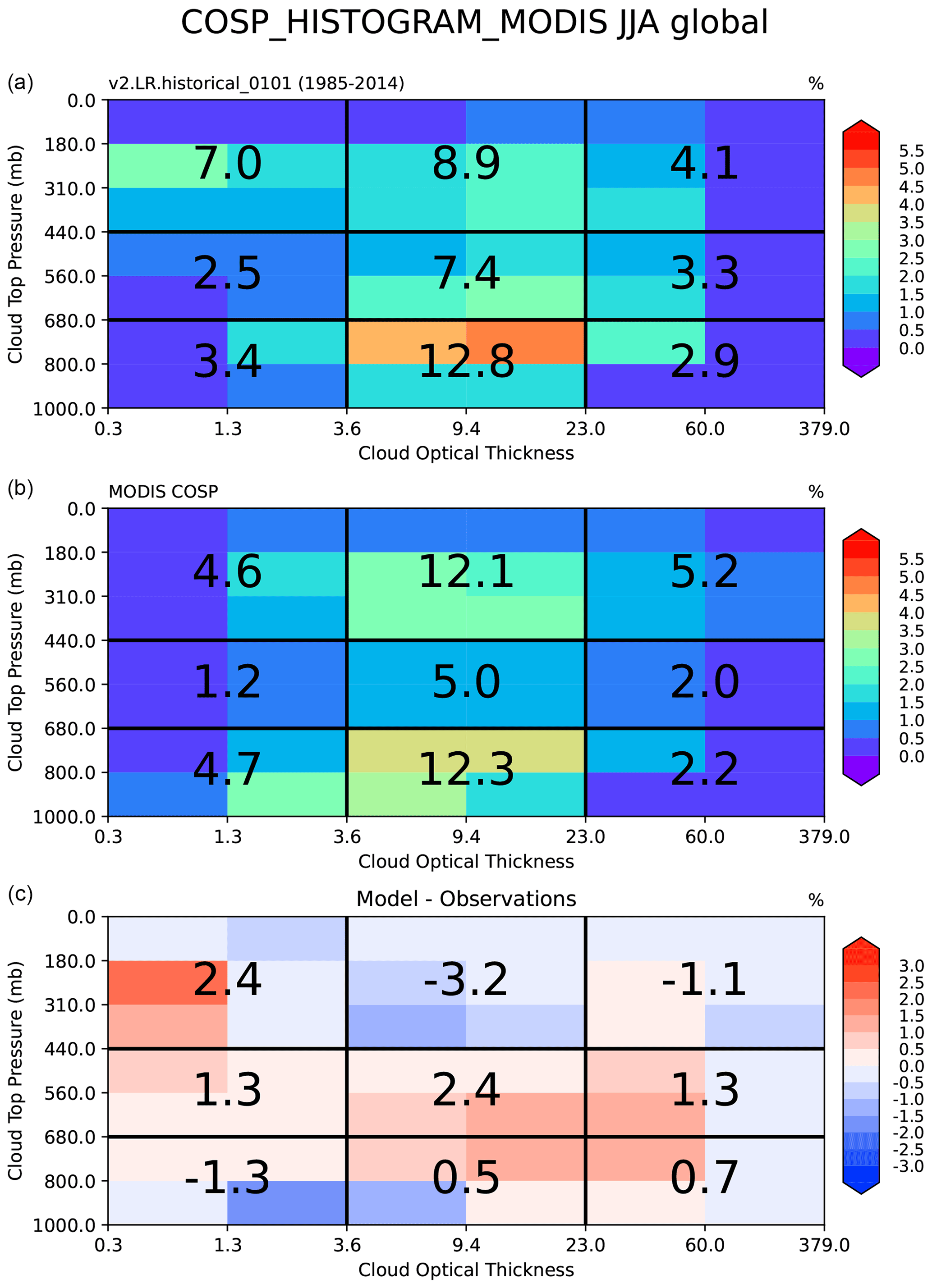
Figure 3 JJA mean distribution of the global-mean cloud fraction as a function of cloud top pressure (vertical axis) and cloud optical thickness (horizontal axis) simulated by the model using the MODIS COSP simulator (a), observed by MODIS satellite (b) and the difference (c).

(Adler et al., 2018)(Rayner et al., 2003)(Kato et al., 2018; Loeb et al., 2018)(Yu et al., 2008)(CFMIP-Observations, 2022)(Wentz and Spencer, 1998)(Kinne et al., 2013)(Large and Yeager, 2009)(Ziemke et al., 2019)(Hersbach et al., 2020)(Dee et al., 2011)(Gelaro et al., 2017)(CFMIP-Observations, 2022)

Table 2 A summary of the basic set of diagnostics in E3SM Diags to evaluate mean physical climate.

3 Overview of available diagnostics

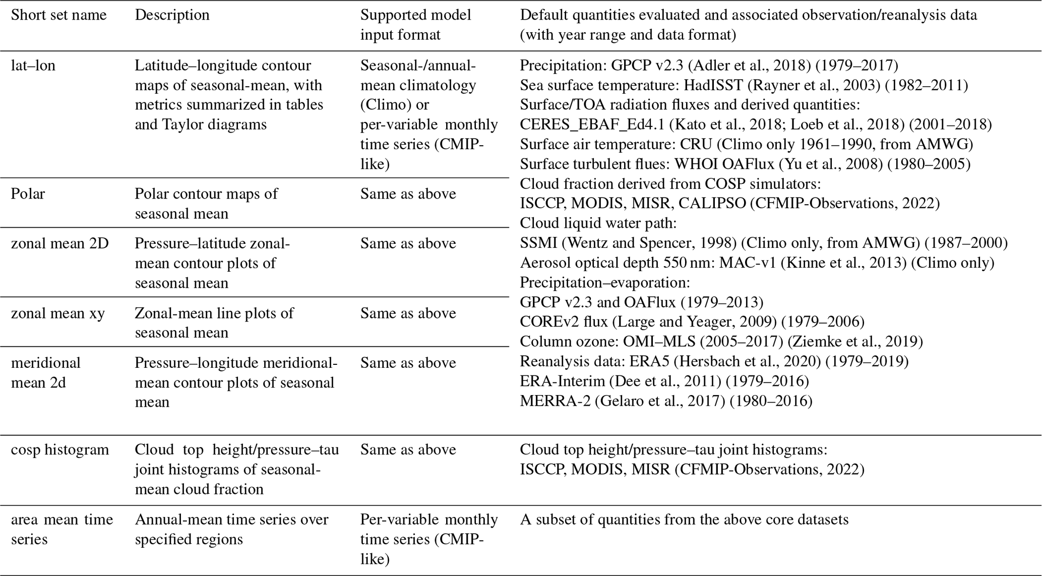
3.1 The core set: seasonal- and annual-mean physical climate

Since the creation of E3SM Diags was inspired by the NCAR's AMWG diagnostics package, the first milestone was a reproduction of key results from AMWG for evaluating model-simulated mean physical seasonal climatology (i.e., DJF: December–January–February, MAM: March–April–May, JJA: June–July–August, SON: September–October–November) and annual mean (ANN). These plot sets are considered to constitute a core set that would be evaluated routinely during model development. This set covers latitude–longitude maps, maps focusing on the north and south polar regions, pressure–latitude zonal-mean contour plots (shown in Fig. 2), pressure–longitude meridional-mean contour plots, zonal-mean line plots, and cloud top height/pressure–tau joint histograms (Fig. 3). Table 2 provides a summary describing these sets. Note that nearly all diagnostics figures included in this paper were extracted from an E3SM Diags (v2.7) run to evaluate simulation from a recently released E3SM version 2 coupled historical run (Golaz et al., 2022). The only exception is Fig. 8, which uses data from a run from one E3SM v2 release candidate where the required output is provided.

Among the core set, the latitude–longitude contour plots that illustrate the global distribution of simulated fields are always being inspected by model developers when comparing simulations with observation and reanalysis datasets. Figure 2 shows a typical three-panel plot that visualizes global latitude–longitude maps, with test/model data in the upper plot, reference/observational data in the middle and the difference plot at the bottom. Metrics including maximum, mean and minimum values are printed on the right upper corner. The test or reference data are regridded (defaulted to conservative regridding) to a lower resolution for both in order to derive the mean bias, RMSE and correlation coefficient of the two datasets as additional metrics to quantify the model fidelity. Also included in the HTML page displaying this figure is the provenance information necessary to produce this figure. In this case the single command line to reproduce the figure is as follows.

e3sm_diags lat_lon
--no_viewer
--case_id 'GPCP_v2.3'
--sets 'lat_lon'
--run_type 'model_vs_obs'
--variables 'PRECT'
--seasons 'ANN'
--main_title 'PRECT ANN global'
--contour_levels '0.5' '1' '2' '3' '4' '5' '6' '7'
 '8' '9' '10' '12' '13' '14' '15' '16'
--test_name '20210528.v2rc3e.piControl.ne30pg2_
EC30to60E2r2.chrysalis'
--test_colormap 'WhiteBlueGreenYellowRed.rgb'
--ref_name 'GPCP_v2.3' --reference_name 'GPCP_v2.3'
--reference_colormap 'WhiteBlueGreenYellowRed.rgb'
--diff_colormap 'BrBG'
--diff_levels '-5' '-4' '-3' '-2' '-1' '-0.5' '0.5'
 '1' '2' '3' '4' '5'
--reference_data_path '/path/to/ref_data/' --test_
data_path '/path/to/test_data/'
--results_dir '/results_path'

This provenance also provides flexibility to generate refined and customized post-run figures. Other than the parameters shown above, more parameters are available to customize this run, including regions, output_format and diff_title. A full list of parameters and available options for each are provided in https://e3sm-project.github.io/e3sm_diags/_build/html/main/available-parameters.html (last access: 12 December 2022).

The core function set supports either ncclimo (Zender, 2008)-processed climatology seasonal- and annual-mean climatology files or per-variable monthly time series files (see Appendix A2 for details on input data requirement), through the specification of Boolean parameters for the input data type. When test_timeseries_input or ref_timeseries_input is set to be true, the climatology computation is performed on the fly for the test or reference input data. With this capability, the standard CMIP data files (i.e., those retrieved from ESGF to local disk) can be accommodated as input data files simply by renaming the files. The built-in derived-variable module takes in CMIP variables and handles variable name and unit conversions.

(Richter et al., 2019)(Hersbach et al., 2020)(Wittenberg et al., 2006)(Bellenger et al., 2014)(Rayner et al., 2003)(Caldwell et al., 2019)(Do et al., 2018)(e.g., Dai, 2001)(Huffman et al., 2007)(Zhang et al., 2020; Schiro et al., 2016)(Zhang et al., 2020)(Balaguru et al., 2020)(Knapp et al., 2010)(e.g., Tang et al., 2021a)

Table 3 A summary of newer diagnostics sets developed since version 2 of E3SM Diags, including key reference papers for diagnostics and data sets. More detailed description is provided in Sect. 3.

Among the core set, cloud top height/pressure–tau joint histograms are special diagnostics that are particularly useful to quantitatively compare simulated properties of clouds with those retrieved by satellite observations (Bodas-Salcedo et al., 2011). Figure 3 shows the comparison of the global mean of cloud fraction distribution, between COSP-simulated model output and observations from the MODIS satellite. Note that this set requires COSP output which is only available when the COSP simulator is enabled during a model run. The implementation of the core diagnostics was completed and released with E3SM Diags version 1. Newer sets developed during version 2 are summarized in Table 3 and introduced in detail in Sect. 3.2–3.8.

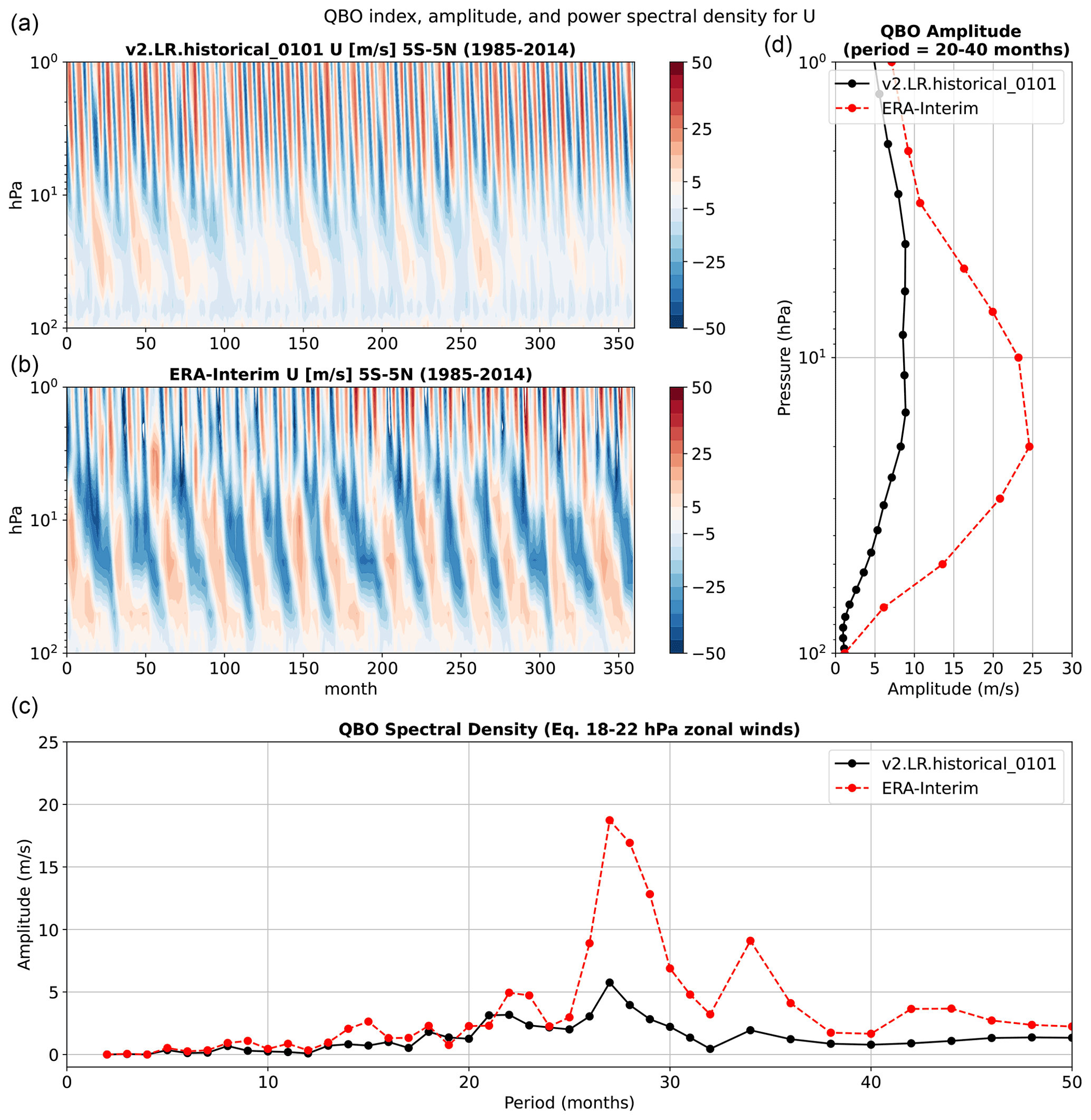
Figure 4 The top left contour plots show monthly mean stratospheric (between 100 and 1 hPa) zonal-mean zonal wind averaged between 5^∘ S and 5^∘ N as a function of pressure and time for model data (a) and ERA-Interim reanalysis data (b). The top right plot (d) shows QBO amplitude derived from the power spectra of stratospheric zonal wind calculated for periods between 20 and 40 months. The bottom plot (c) shows power spectra of stratospheric zonal-mean zonal wind at a pressure level between 18 and 22 hPa. Model data are averaged over 51–60 simulated years (black lines), and ERA-Interim reanalysis data are averaged over the years 2001 to 2010 (red lines).

3.2 Quasi-biennial oscillation (QBO)

The quasi-biennial oscillation (QBO) is an important mode of variability which refers to a roughly 28-month oscillation of easterly and westerly winds in the equatorial stratosphere that propagates downwards from 5 hPa down to 100 hPa (Baldwin and Tung, 1994). The QBO has been found to impact extratropical (Thompson et al., 2002; Marshall and Scaife, 2009; Garfinkel and Hartmann, 2011) and tropical climate and variability (Marshall et al., 2016). Furthermore, an ensemble of QBO-resolving models reveals that the QBO teleconnections potentially influence the polar vortex (Anstey et al., 2021). Despite its wide-ranging influence on tropospheric phenomena, most climate models struggle to capture key signatures of the QBO (Butchart et al., 2018). Although an ensemble of QBO-resolving models shows that more and more models are capable of simulating the QBO, the amplitude of this phenomenon is shifted upwards (Richter et al., 2020).

The QBO diagnostics, as described in Richter et al. (2019), use monthly mean output of equatorial (5^∘ S–5^∘ N) zonal winds from the model to determine how well the model captures the period and amplitude of the equatorial zonal stratospheric wind oscillations. Three plots comprise the diagnostic (Fig. 4): a time-versus-height contour plot of the zonal winds shows whether the model qualitatively captures the downward propagation of easterlies and westerlies from 1 hPa down to 100 hPa. The height-resolved amplitude of zonal wind oscillations over the typical period of the QBO allows quantitative comparisons of the modeled and observed amplitude of the QBO. Finally, the QBO spectra, which capture the amplitude of the oscillation as a function of the period for zonal winds between 18 and 22 hPa, help determine whether the QBO period is correctly simulated in the model. For the observational reference, zonal winds from ERA5 reanalysis (Hersbach et al., 2020) are used.

Figure 4 shows the time series of the equatorial zonal winds in the stratosphere simulated by the E3SMv2 model. While the model captures the downward propagation of the equatorial zonal winds in the stratosphere, the simulated easterly phase is too weak. The amplitude of the QBO, measured as the wind amplitude within periods of 20–40 months, is too weak as compared with the ERA-Interim observations. The model simulation reveals that the peak period of the simulated QBO is 28 months, which is similar to what has been observed, although the amplitude is too weak.

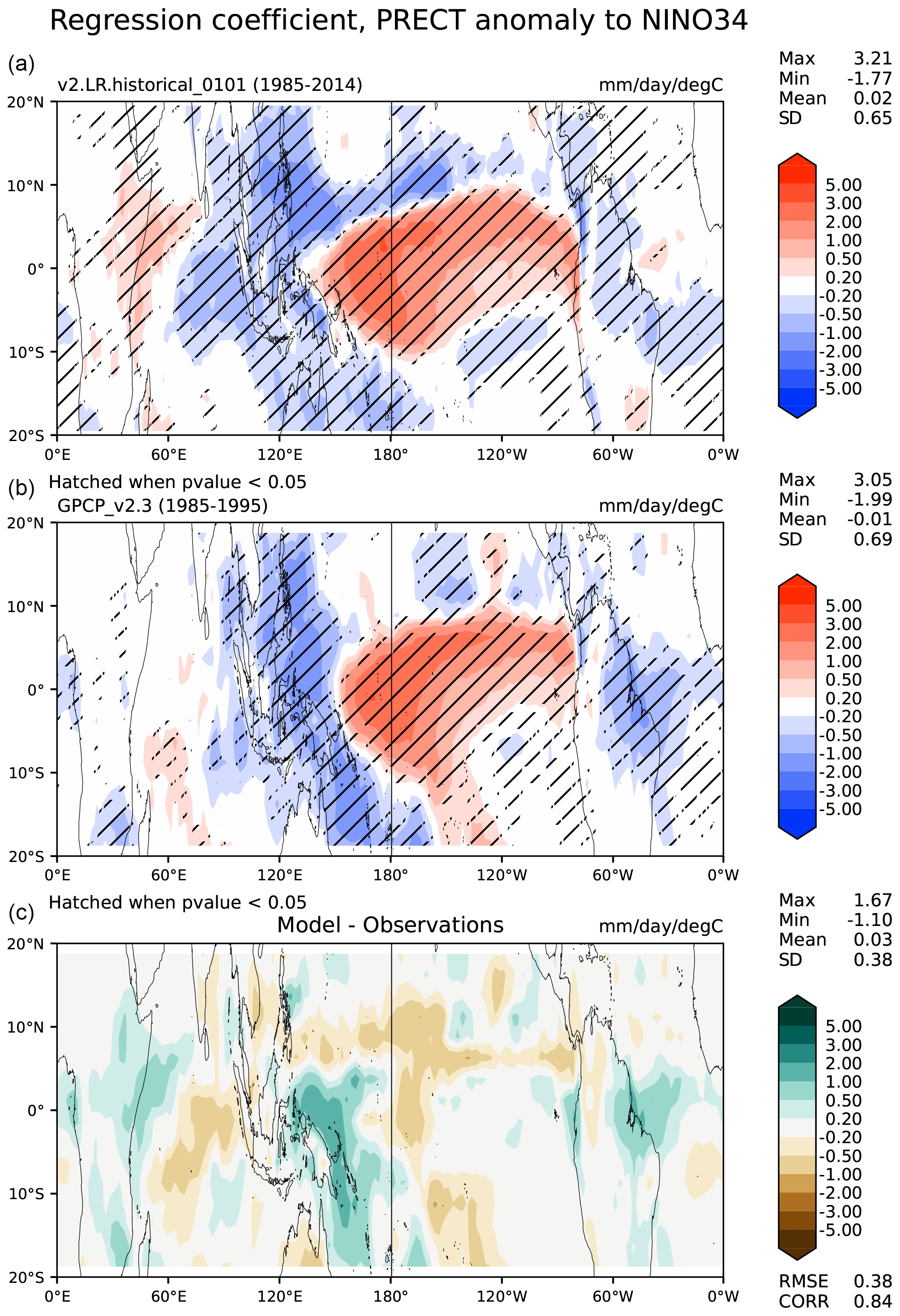
Figure 5 Plots of the linear regression coefficient of the total precipitation rate on monthly Niño sea surface temperature (SST) anomalies in the 20^∘ N and 20^∘ S latitude band. Panel (a) shows one version of E3SM data using monthly output for 51–60 simulated years. Panel (b) shows the same variable but uses the precipitation rate from the satellite-based Global Precipitation Climatology Project (GPCP) v2.3 data and monthly Nino 3.4 SST anomalies (Rayner et al., 2003) for the 2001–2010 period. Hatching in the top two plots indicates a confidence level in the regression greater than 95 %. Panel (c) shows the difference between the model and the observations.

3.3 El Niño–Southern Oscillation (ENSO) diagnostics

ENSO is the dominant mode of climate variability over seasonal to interannual timescales in the global climate system. Realistic simulation of ENSO variability is important for both climate prediction and projection. ENSO diagnostics include its teleconnections and process-based evaluations of atmosphere–ocean feedbacks. These diagnostics were first implemented within the A-PRIME package (Evans et al., 2017) and later incorporated into E3SM Diags. For evaluation of model-simulated ENSO, we compute time series of the widely used Nino 3, Nino 3.4 and Nino 4 indices and the equatorial Southern Oscillation Index. For evaluation of ENSO and its teleconnections, we provide a spatial distribution of the regression of a list of variables – namely, surface precipitation, sea-level pressure, zonal wind stress and surface heat flux and its components – over the Niño region SST anomalies (departures from the normal or average sea surface temperature conditions). This set of analyses is used to evaluate the response of the atmosphere to the SST anomalies and therefore provides insights into model tuning for better ENSO representation in coupled simulations (e.g., Wittenberg et al., 2006). If the atmospheric model generates a reasonable response (compared to the observed SST data), then the model is likely to generate a better ENSO signal in coupled runs. An example of this diagnostic is shown in Fig. 5 for precipitation, indicating that the candidate model simulates a credible local and remote precipitation response to ENSO. We use Student's t test to establish the statistical significance of the regression coefficients.

Additionally, we also include an estimate of the Bjerknes feedback simulated by the model as the slope of the linear fit to the scatterplot of SST monthly anomalies over the Niño 4 region against the zonal wind stress monthly anomalies over the Niño 3 region (e.g., Bellenger et al., 2014). This estimates the impact of remote tropical Pacific zonal winds on eastern Pacific SSTs. We use a similar metric to compute the surface heat flux–SST feedbacks, another important atmosphere–ocean mechanism modulating the ENSO development cycle (e.g., Bellenger et al., 2014), for the net surface heat flux and each of its components, namely latent heat flux, sensible heat flux, shortwave heat flux and longwave heat flux. We capture the nonlinearity of these feedbacks by computing the slope of the linear fit to the scatterplots separately for positive and negative anomalies. Data from ERA-Interim are used for the heat flux components and surface wind stress.

Finally, it would be useful to evaluate the time evolution of ENSO and its remote impacts in the models. In future development, it is planned to include a lead–lag correlation/regression analysis of several variables globally against the Nino 3.4 index, with the Nino 3.4 index leading the variables by −8, −4, 0, 4 and 8 months.

3.4 Streamflow diagnostics

Seasonal variability in the streamflow discharge is an important metric often used to characterize geographic differences and climate change impacts in streamflow (e.g., Dettinger and Diaz, 2000; Caldwell et al., 2019). Given that the streamflow combines the heterogeneity and complexity contributed from both atmosphere and land components, streamflow seasonality is also commonly used to study how climate signals are translated through land to the river discharge (e.g., Petersen et al., 2012; Berghuijs et al., 2014). In the E3SM Diags Package, we benchmark the peak month and the seasonality index of the streamflow discharge simulated by the E3SM river model (MOSART). The reference dataset selected is the Global Streamflow Indices and Metadata Archive (GSIM; Do et al., 2018), which includes daily streamflow discharge time series at more than 30 000 gauge locations worldwide.

One of the challenges commonly faced in streamflow comparisons is how to accurately georeference the gauge locations from simulated results which are based on different spatial resolutions and/or different river network delineations. In this diagnostics set, we used drainage area as the reference value to identify each gauge on the simulated streamflow discharge field. The tool allows the gauge location to move within a defined radius from the actual coordinates to better match the drainage area between the observation and the simulation. It will automatically remove the gauge from the comparison if the drainage area bias is larger than a pre-defined threshold. This scale-free approach has been successfully applied in Caldwell et al. (2019).

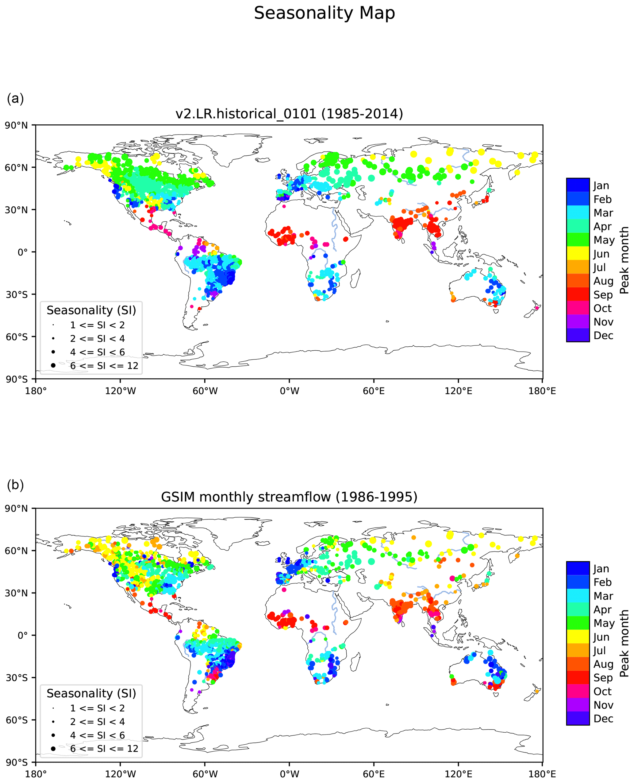
Figure 6 Seasonality of streamflow discharge over gauge locations with the peak month of the hydrograph (color of the dots) and seasonality index (SI, size of the dots) for model-simulated streamflow (a) and for GSIM gauge observations (b).

Figure 6 shows an example of the streamflow diagnostic results by comparing the seasonality between E3SMv2 and observations at globally distributed gauge locations. The color of the dots indicates the peak month of the averaged monthly streamflow time series, and the size indicates the seasonality index (SI) of the streamflow. The SI quantifies the level of seasonal variations in the hydrograph; it ranges from 1 to 12, with 1 indicating a uniformly distributed hydrograph across the year (i.e., no seasonal variation) and 12 indicating that peak streamflow occurs in a single month, while the rest of the months are equal (i.e., the strongest possible seasonal variability). The formula for SI calculations can be found in Golaz et al. (2019). The results suggest that the model reasonably captured the peak season of the streamflow in most of the areas except the northwest of North America and western Europe.

In addition to a seasonality map, the streamflow diagnostic set, by default, offers maps and scatterplots comparing annual-mean streamflow discharge over gauge locations between GSIM observations and simulated streamflow.

3.5 Diurnal cycle of precipitation

Metrics and diagnostics for the diurnal cycle of precipitation are often used to benchmark climate models (Covey et al., 2016). The representation of the diurnal cycle of precipitation is largely linked to moist convection parameterization (Xie et al., 2019). Even the most state-of-the-art climate models have shown difficulties in capturing the correct peak time and amplitude of the daily precipitation cycle (Tang et al., 2021b; Watters et al., 2021). In particular, the eastward propagation of mesoscale convective systems is poorly represented by climate models.

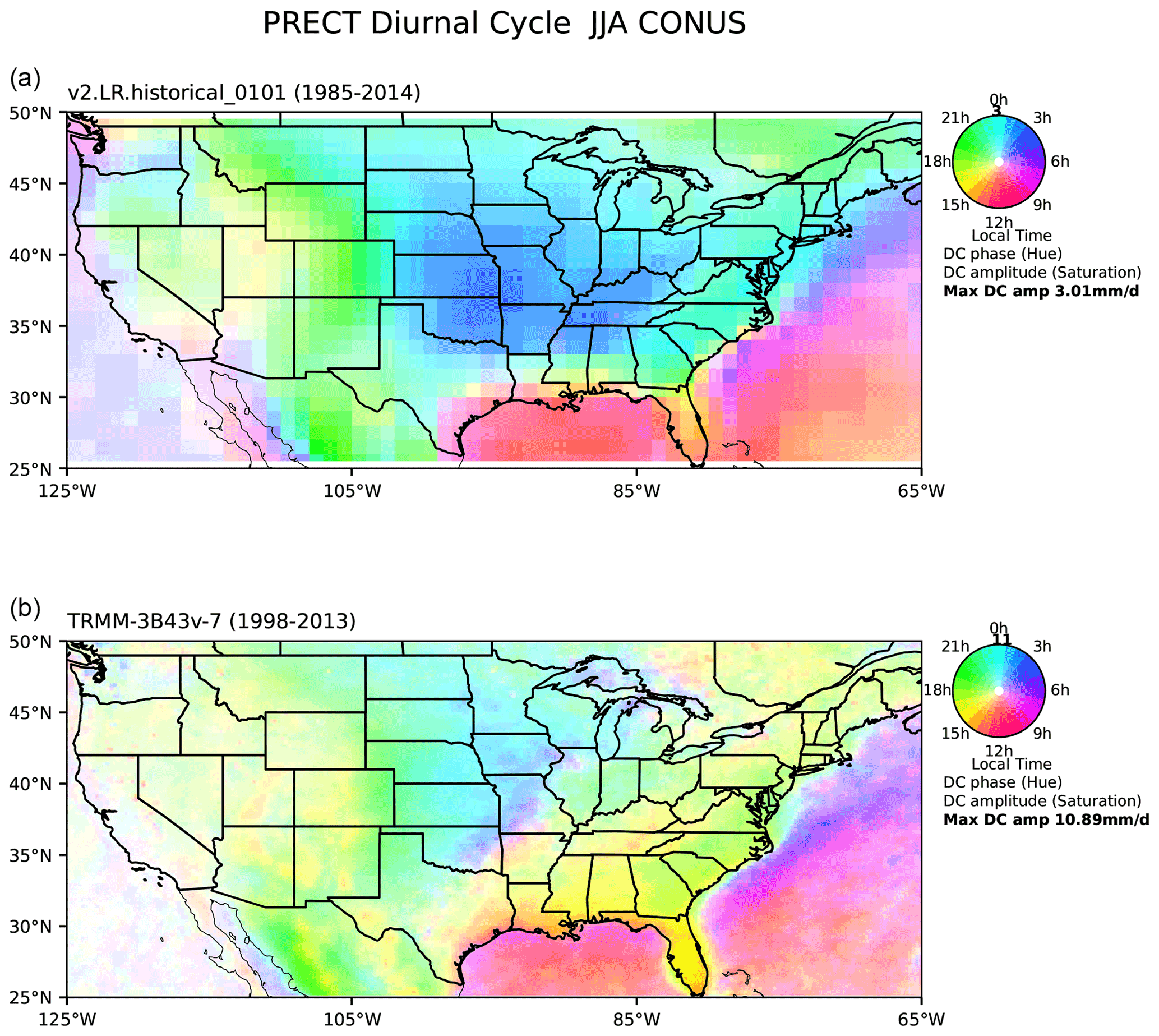
Figure 7 Phase (color) and amplitude (color saturation) of the first diurnal harmonic of precipitation over CONUS for the composite JJA mean of 3-hourly data for model data from 51–60 simulated years (a) and TRMM 3B43V7 from the years 1998–2003 (b).

Harmonic analysis is a traditional way to evaluate diurnal variability (Dai, 2001). In the E3SM Diags implementation, as a pre-processing step, ncclimo is used to first average the time series into a composite 24 h day for each month/season and annual mean, and then Fourier analysis is applied to obtain the first harmonic component, as described in Covey et al. (2016). The local times of the precipitation peak (color hue) and amplitude (color saturation) of the first harmonic are displayed on a map (Fig. 7).

As shown in the lower panel (TRMM 3B43V7) in Fig. 7, over the central United States, there is a clear signal of eastward precipitation propagation originating from the lee of the Rocky Mountains in the late afternoon to a late evening or midnight peak over the central US. Rainfall generated from these organized mesoscale convective systems accounts for the majority of the midsummer precipitation between the Rockies and the Appalachians (Carbone and Tuttle, 2008). The test model evaluated in the top panel of Fig. 7 captures the eastward propagation, but the movement appears to be too slow, thus resulting in a later (early morning) peak over the central USA. The peak time over the southeastern USA is also several hours too late. In general, the model simulated much lower diurnal amplitude than observed. A set of standard regions that covers the globe, the Amazon, the western Pacific and the contiguous USA (CONUS) are enabled in E3SM Diags for comparing diurnal cycle metrics with reference datasets.

One caveat of this analysis is that it only provides meaningful information for locations and seasons when most of the daily variability can be explained by the first harmonic. A complementary map (e.g., Fig. 10 in Xie et al., 2019, and Fig. 3 in Pritchard and Somerville, 2009) that gives explained variance will be included in future releases.

3.6 ARM diagnostics

The US Department of Energy's Atmospheric Radiation Measurement (ARM) user facility obtains long-term, high-frequency, ground-based measurements of atmospheric data at various fixed locations around the globe. These state-of-the-art observational data, which include three-dimensional measurements, provide a unique resource to understand aerosol, cloud and precipitation processes in diverse climate regimes and have led to significant improvements in their representations in climate models. To facilitate the use of the comprehensive ARM observations in climate model evaluation, the ARM data-oriented metrics and diagnostics package (ARM Diags) (Zhang et al., 2020) has been developed, which allows users to quickly compare their model results with the climatology and time-series files generated from the ARM data at multiple ARM sites.

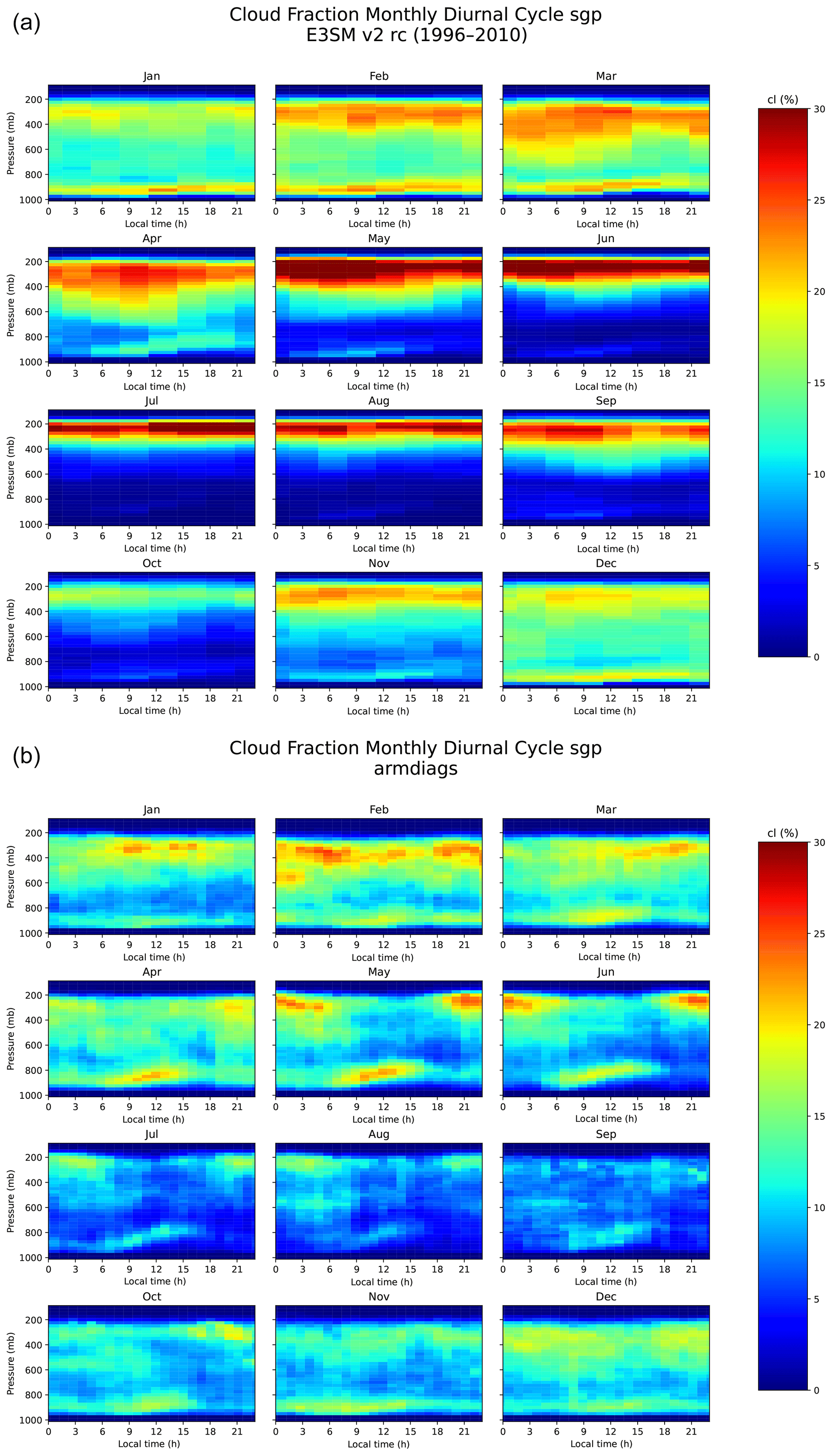
Figure 8 Monthly mean cloud fraction diurnal cycle comparing model data (a) and ARM observations (b).

The evaluation set in the current version of ARM Diags (version 2.0) includes the seasonal mean and annual cycle of several atmospheric variables (e.g., surface air temperature, precipitation, radiation fluxes and surface turbulent fluxes), the convective onset metrics showing the statistical relationship between the precipitation rate and column water vapor (Schiro et al., 2016), along with the diurnal cycle of precipitation and vertical profiles of the cloud fraction. Among these, the convection onset and diurnal cycle diagnostics are particularly useful to help understand how the parameters and related physical processes are represented in the model. For example, the common model bias in the representation of the physical processes controlling the life cycle of clouds can be clearly recognized in the metric of the diurnal cycle of the vertical cloud fraction. As shown in Fig. 8b, a shallow-to-deep-cloud transition is observed over the ARM Southern Great Plains (SGP) site during the spring to summer seasons (April–August) while the diurnal cycle of the vertical cloud fraction simulated in E3SMv2 is featured with persistent high clouds (Fig. 8a). This model bias is highly relevant to parameterization deficiencies in convection, meaning that the deep convection scheme is too easily triggered in the model.

With the ARM Diags having now been integrated into E3SM Diags, users can routinely evaluate the performance of the E3SM simulation against the ARM observations at multiple ARM sites, including the SGP site; the North Slope of Alaska (NSA) Barrow site; and the Tropical Western Pacific (TWP) Manus, Nauru and Darwin sites. Consequently, ARM Diags supports model evaluation and enhancement in continental, marine and high-latitude environments. The extension of current ARM-Diags to the Eastern North Atlantic (ENA) site and the ARM Mobile Facility (MAO) at Manaus, Amazonia, Brazil, is under development and will be available in the next version. Given that cloud and aerosol feedbacks remain the largest source of uncertainty in climate sensitivity estimates, in future versions of ARM Diags standardized analysis tools and associated ARM observational datasets for aerosol–cloud interaction (ACI) metrics will be implemented as a new process-oriented diagnostics suite.

3.7 Tropical-cyclone analysis

Tropical cyclones (TCs) are arguably the most destructive weather systems in the global tropics and sub-tropics and impact millions of people annually worldwide (Emanuel, 2003). They may also play an active role in modulating the planet's climate system (Korty et al., 2008; Fedorov et al., 2010). As climate models are pushed to the resolutions needed to resolve these features, it becomes important to evaluate their ability to accurately simulate TCs and their environment. To this end, TC metrics that quantify some of their properties have been included in E3SM Diags. In E3SM, TCs are tracked using model output at 6-hourly frequency and using TempestExtremes, scale-aware feature tracking software (Ullrich et al., 2021). TC-like vortices are initially identified using a minimum sea-level pressure condition. We then check to see if a closed contour exists around the vortex center within a great circle distance of 4^∘, where the pressure increases by at least 300 Pa from the center to any point on the contour. Next, to ensure that the vortex center has a warm core, we check to see whether the anomalous temperature, averaged over 200–500 hPa, decreases by 0.6 K in all directions within a great circle distance of 4^∘ from the center. Finally, we check to see whether there are at least six 6-hourly track locations where the maximum surface wind speed within the closed contour exceeds 17.5 m s⁻¹, which corresponds to the minimum value for “tropical-storm” strength. The threshold values used for sea-level pressure and upper-level temperature are based on an optimal parameter search to match reanalysis to observations (Zarzycki and Ullrich, 2017). For further details regarding the detection of TCs in E3SM, see Balaguru et al. (2020).

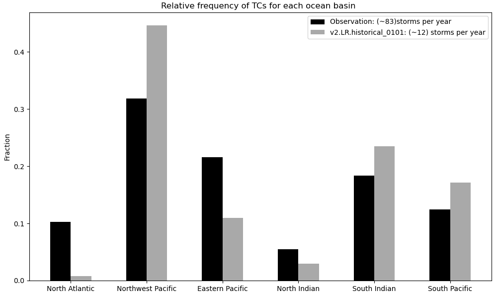
Figure 9 Climatological mean TC relative frequency for various basins, from model data (black) and observations (grey). The values for the respective global annual-mean TC frequencies are indicated in the legend. Observed TC data are from IBTrACS (Knapp et al., 2010) for the period 1979–2018.

Various TC characteristics can be examined through E3SM Diags, including their frequency, spatial distribution, seasonality, track density and total activity represented by the accumulated cyclone energy (ACE). Also included are African easterly waves, which are well-known precursors for some TCs in the Atlantic and the eastern Pacific (Thorncroft and Hodges, 2001). For instance, Fig. 9 shows the relative frequency of TCs in various basins. Overall, the model simulates around 6 TCs per year globally, which is a substantial underestimation when compared to observations (∼ 80 TCs per year). Previously, we have seen that at an approximate resolution of 1^∘, the model produced nearly 15 TCs on average (Balaguru et al., 2020). Considering this, as well as that the current model resolution is approximately 1.5^∘, the model bias in TC frequency is not surprising. A notable aspect of TC relative distribution (Fig. 9) is the significant negative bias in the North Atlantic, which is likely related to the under-representation of African easterly waves in coarse-resolution models (Camargo, 2013; Balaguru et al., 2020).

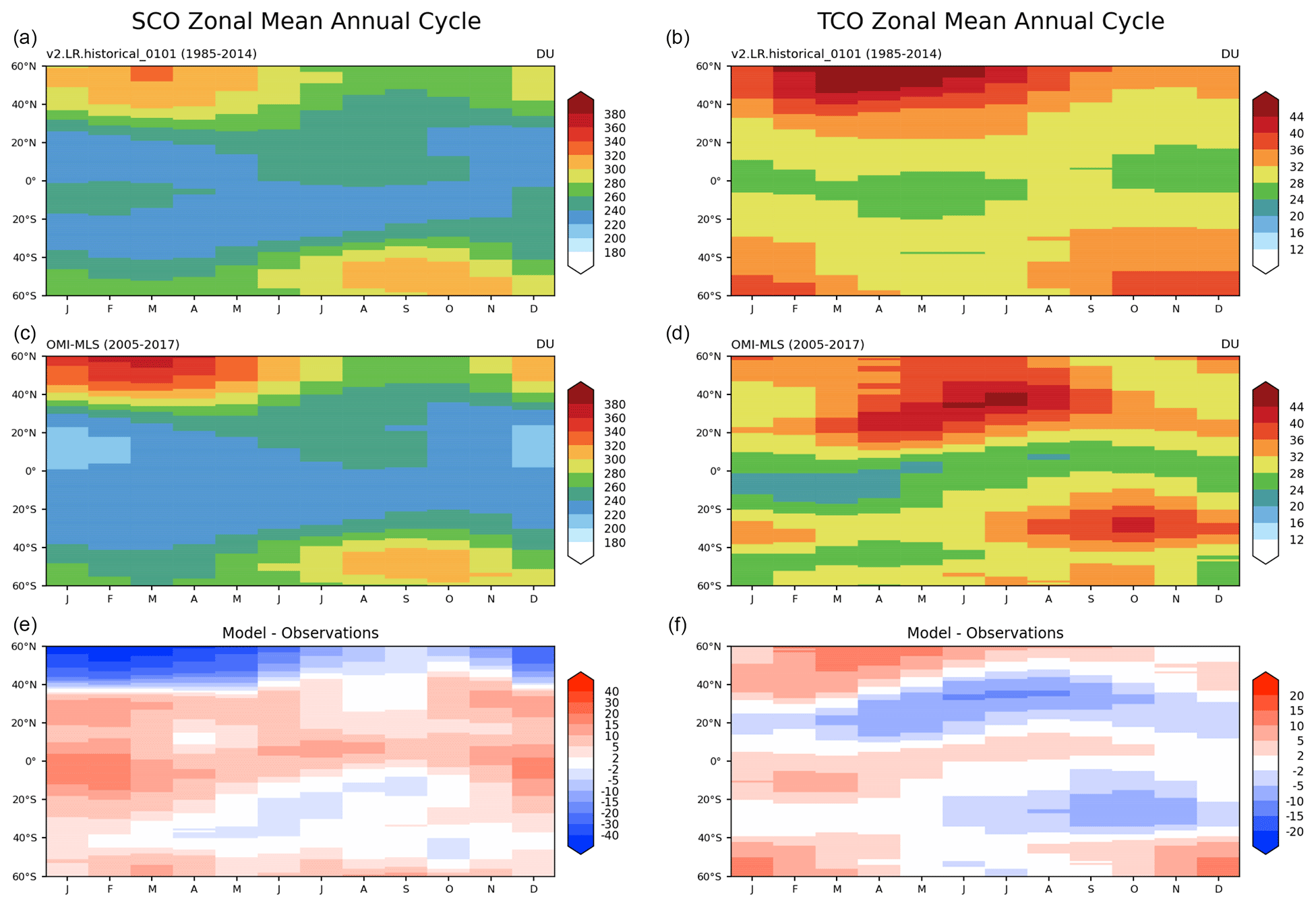
Figure 10 Multi-year mean annual cycle of the zonal-mean stratosphere column ozone (SCO; a, c, e) and troposphere column ozone (TCO; b, d, f) in Dobson units. OMI–MLS observations for the years 2005–2017 are shown in the middle row.

3.8 Annual-cycle zonal mean

Along with describing the interactive atmospheric chemistry package for E3SM, Tang et al. (2021a) aimed to establish a set of standard climate–chemistry metrics for simulation evaluation, focusing on the stratospheric ozone in E3SMv1 and E3SMv2. Previous studies have normally looked at the total column ozone, which cannot differentiate data from the stratosphere and troposphere. Here (see Fig. 10) we separate the total ozone column into stratospheric and tropospheric components as their driving mechanisms are different and hence they can have different characteristics, such as in variability and trend.

The stratospheric column ozone (SCO) observational data used in E3SM Diags are derived from ozone measurements from the Aura Ozone Monitoring Instrument–Microwave Limb Sounder (OMI–MLS) data (Ziemke et al., 2019). The model–observation comparisons are limited to 60^∘ S to 60^∘ N, where the satellite observations from OMI and MLS have good qualities all year round. The annual-cycle zonal-mean plots from multiple years of data show low SCO at the tropics and high SCO at middle to high latitudes. In the Northern Hemisphere, SCO peaks during the boreal springtime, while in the Southern Hemisphere it peaks in the austral springtime. This SCO pattern is determined by both the stratospheric photochemistry and circulation. Therefore, a good match between models and observations with this SCO metric suggests a good representation of the climatology of photochemistry and dynamics in the modeled stratosphere.

This metric is the first step towards incorporating atmospheric chemistry diagnostics into E3SM Diags. More new metrics from Tang et al. (2021a) will be incorporated into future versions to facilitate the evaluation of other chemistry aspects, such as the standard deviation of the SCO anomaly as a function of latitudes, Taylor diagrams of the zonal-mean climatology and ozone hole metrics.

4 Application of E3SM Diags

E3SM Diags was designed to provide standalone model-to-model and model-to-observation comparisons between two sets of data on regular latitude–longitude grids. Over time, several applications for the E3SM Diags module have been invented to streamline its use for different scientific purposes. This section provides a few use cases of running E3SM Diags.

4.1 zppy

As described in Appendix A2, post-processing native-format E3SM output is required before running E3SM Diags. A separate Python tool zppy (pronounced “zip-ee”/“zippy”) (https://github.com/E3SM-Project/zppy, last access: 12 December 2022) has been developed to automate these post-processing steps as well as handle E3SM Diags tasks. zppy is highly customizable, allowing users to specify settings at multiple levels (i.e., for general input and output information and for each sub-task) in the configuration file or to apply to as many or as few tasks as necessary. Because of this, users can easily run E3SM Diags on multiple different time periods and with specific diagnostic sets. For example, a user could run E3SM Diags on the last 30 years of climatology data, despite generating many more years of data in the climatology task.

zppy launches a batch job for each task. If multiple year sets are defined (e.g., 1–50, 50–100), then a single task may launch multiple jobs, one for each year set. zppy submits these jobs for execution by Slurm, taking into account any job dependencies.

Figure 11 E3SM Diags dependencies that zppy handles.

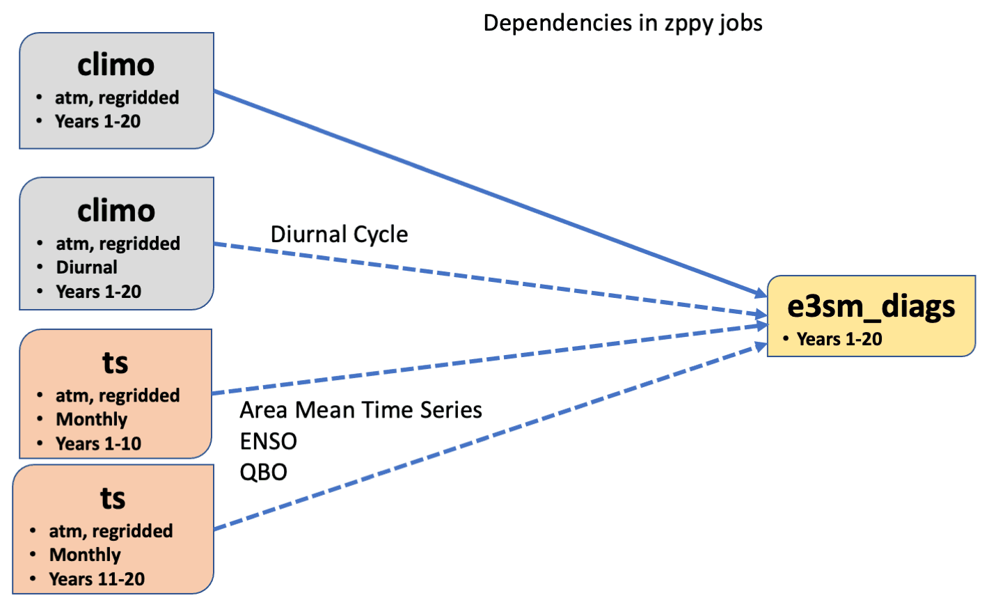
With a single user-created configuration file, zppy will determine which climatology and time series tasks need to complete first, run E3SM Diags, and finally copy over the plots to the machine's web server. This enables significant streamlining in running E3SM Diags with E3SM data. Figure 11 demonstrates an example of pre-processing dependencies that zppy handles before running e3sm_diags. The pre-processing tasks include generating regridded climatology from monthly output, mean diurnal cycle climatology from 3-hourly output and regridded monthly time-series files, as input for various E3SM Diags sets. The workflow for running E3SM Diags through zppy is provided as https://github.com/E3SM-Project/e3sm_diags/tree/main/examples (last access: 12 December 2022).

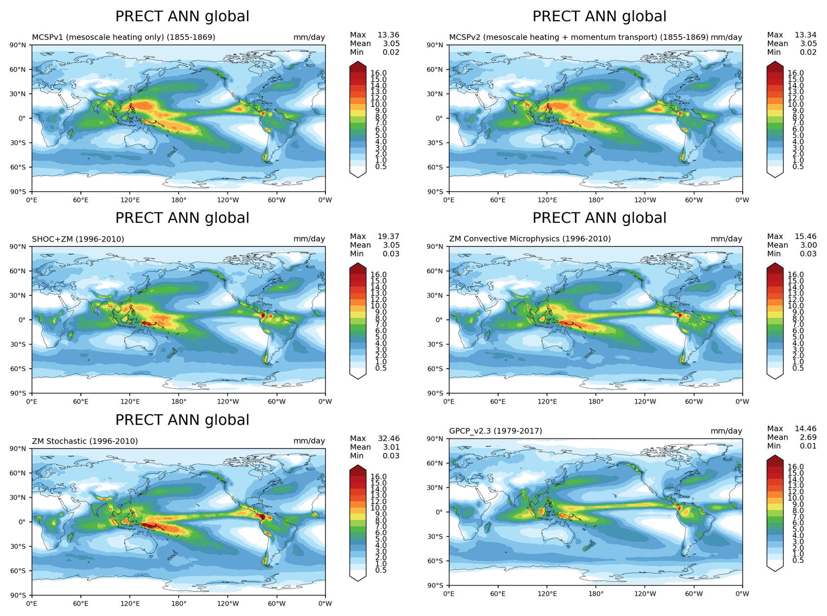
Figure 12 A multi-panel-view figure generated by IICE to compare global annual-mean precipitation maps based on five individual E3SM Diags runs on simulation data with each featuring a distinct convection scheme.

4.2 IICE (Interface for Intercomparison of E3SM Diag)

E3SM Diags leverages web browsers to pair various diagnostics of a model simulation and reference data for comparison. Frequently, during both model development and evaluation stages, we are faced with many such comparisons – with observations or control or contrasting simulations. In the same spirit of the design for E3SM Diags, the online Interface for Intercomparison of E3SM Diags (IICE) has been developed to enable simultaneous comparison of arbitrary number of diagnostics produced by E3SM Diags. The interface keeps the user side configuration to a minimum. No installation is required; no new plots are generated. Users of IICE only need to specify the URLs to the existing E3SM Diags' viewers for the simulations to be compared as well as optional corresponding labels. The plot sets are organized in the same format as the standard E3SM Diags (Fig. 12). To save the need to re-enter the URLs and labels, the links to a specific customized intercomparison – from the index pages for the plots sets to the diagnostics of individual fields – can be recorded for convenient sharing. IICE is a standalone online interface. The IICE interface is hosted at https://portal.nersc.gov/project/e3sm/iice (last access: 12 December 2022), along with a demonstration of how to use the interface for intercomparison of E3SM Diags-computed diagnostics.

4.3 CMIP data intercomparison

As mentioned in E3SM Diags' input data requirement in Appendix A2, E3SM Diags can ingest CMIP-formatted input files. Therefore, the same set of plots used to evaluate E3SM can also be generated for all available CMIP models for easy apple-to-apple comparisons. We demonstrate the use of E3SM Diags running alongside the CMIP6 data archive available locally at the Lawrence Livermore National Laboratory (LLNL) ESGF node to provide a model intercomparison. The workflow includes aggregating input CMIP data files using the Climate Data Analysis Tools (CDAT) cdscan utility, running E3SM Diags over the requested experiments and realization of specified models, and finally generating a web page with tables summarizing high-level metrics (i.e., RMSE) performance for a number of selected fields. An example can be found here: https://portal.nersc.gov/project/e3sm/e3sm_diags_for_cmip/ (last access: 12 December 2022); one can select the field and sort the columns. The numbers link directly to the actual E3SM Diags figures. The full set of figures is linked to the realization. This workflow is also documented in the E3SM GitHub repo, and it can be run routinely to evaluate candidate versions of E3SM and compare their performance with other CMIP models. We plan to regularly update this page to keep it current with newer submissions to the CMIP archive.

5 Summary and future work

E3SM Diags is an open-source Python software package that has been developed to facilitate evaluation of Earth system models. Since its first software release on GitHub in September 2017, the package has evolved rapidly and has now become a mature tool with automated CI/CD systems and consolidated testing and provenance tracking. It is being used routinely in the E3SM development cycle, and it also has the flexibility to process and analyze CMIP-compliant data. It has been extended significantly beyond the initial goal to be a Python equivalent of the NCL AMWG package. More project and community-contributed diagnostics sets were implemented through the flexible and modular framework during version 2 of the software development. Multiple applications of the E3SM Diags module were invented to fit diverse use cases from the science community.

Moving ahead, E3SM Diags will continue to evolve as one of the main evaluation packages for component models of E3SM. While expanding on the functionality of each existing set (as outlined in Sect. 3), several parallel efforts with new sets are ongoing to meet requirements from science groups. Some prioritized items include a suite of metrics focusing on precipitation and related water cycle fields, analysis of tropical sub-seasonal variability, and additional support for land and river components.

The next phase of development will also bring enhancements to observational data into focus. At present, the selection of the “best” reference observation dataset for each analysis is based on domain experts' guidance as well as recommendation from resources like NCAR's Climate Data Guide (Schneider et al., 2013). The selected datasets are being updated when data providers release extensions or new versions (e.g., CERES_EBAF_Ed4.1 in place of Ed4.0). We aim to build a more robust system that includes and documents multiple sources (when available) of expert-recommended reference data streams with quantitative uncertainty information attached to guide interpretation of results.

Regarding technical enhancements, addressing performance challenges emerging from application to large ensembles and high-resolution model data will be a focus area. Effort was spent on scoping out a cross-node parallelism approach. We also plan to move away from the soon-to-be-retired CDAT package, the current data I/O and analysis dependency and instead utilize newly emerging tools based on Xarray and Dask (e.g., xCDAT, https://github.com/XCDAT/xcdat, last access: 12 December 2022), which are also expected to make the software more performant.

Lastly, E3SM Diags has a framework that is flexible to extend. We provide a developer's guide as resource for community contributions. In the meantime, we aim to provide modules that can be straightforwardly ported or used for different evaluation capabilities (e.g., via the aforementioned Coordinated Model Evaluation Capabilities, CMEC).

Appendix A: General guide for running E3SM Diags

This section provides general guidance to set up and run the package.

A1 Installation

E3SM Diags is available as a Conda package that is distributed via the conda-forge channel. Two versions of YAML files that specify the package dependencies are maintained: one referring to the latest stable release of E3SM Diags and the other referring to the development environment. Using the later YAML file to create the development environment requires building the package from its code repository. A detailed installation guide can be found in https://e3sm-project.github.io/e3sm_diags/_build/html/main/install.html#installation (last access: 12 December 2022).

Alternatively, on all of the standard E3SM computational platforms (e.g., the National Energy Research Scientific Computing Center, NERSC), the E3SM project supports a single unified Conda environment (E3SM Unified) that includes nearly all tools for post-processing and analyzing model E3SM output. One can access E3SM Diags by activating E3SM Unified on supported machines following activation instructions (https://e3sm-project.github.io/e3sm_diags/_build/html/main/install.html, last access: 12 December 2022). The observational datasets are maintained on these machines, without the need to download them from the E3SM input data server. For users who do not have access to the E3SM-supported platforms, the setup on a Linux/macOS system would require both installation and downloading the observational datasets (see “Data availability” section for location).

A2 Input file requirement

Additional pre-processing may be needed depending on the input data being analyzed. In general, input files are expected to be on a regular grid, with some exceptions (e.g., for TCs and single-grid output from ARM sites). Two model conventions are currently supported by E3SM Diags: E3SM (potentially also CESM, from which E3SM was branched) and CMIP conventions. Originally, this package started by mimicking AMWG; therefore the input files required are monthly (12 files), seasonal (4 files) and annual-mean (1 file) climatology files with all model variables included in each of the 17 files post-processed from the native CESM Community Atmosphere Model (CAM) or E3SM Atmosphere Model (EAM). Starting from E3SM Diags version 1.5, support for monthly time series and generating climatologies on the fly has been implemented. This change additionally opened up the possibility for integrating more analyses that focus on variability and trends.

The design decision to handle data on regular latitude and longitude grids, instead of on the E3SM native grid, is to support more general use of this package and accommodate other models following CMIP conventions. However, this also means that remapping and reshaping must be performed as a pre-processing step for E3SM native model output. Examples of scripts to pre-process native EAM output are provided under e3sm_diags/model_data_preprocess. The following three scripts serve as post-processing based on specified sets:

• postprocessing_E3SM_data_for_e3sm_diags.sh, using NCO to remap and generate climatology files and time-series files for required variables;

• postprocessing_E3SM_data_for_TC_analysis.sh, using TempestRemap and TempestExtremes to generate TC tracks;

• postprocessing_E3SM_data_for_single_sites.py and postprocessing_E3SM_data_for_single_sites
.py, to generate single grid time series from ARM sites.

To evaluate one-variable-per-file netCDF files (i.e., those from the CMIP archive), one additional step is needed to bring the file name and structure into compliance with E3SM Diags requirements. Specifically, files must be renamed to the NCO style (<variable>_<start-yr>01_<end-yr>12.nc, e.g., renaming tas_Amon_CESM1-CAM5_historical_r1i1p1_
196001-201112.nc as tas_196001_201112.nc). All files must be placed into one input data directory. Symbolic links can be used to prevent data duplication. Any sets listed in Tables 2 and 3 that support CMIP-like variables can be used to evaluate CMIP files. More details on input data requirements can be found at https://e3sm-project.github.io/e3sm_diags/_build/html/main/input-data-requirement.html (last access: 12 December 2022).

A3 Configuration and execution

The most common method to configure and run E3SM Diags is to use a configured Python script that calls e3sm_diags executable. This script contains pairs of keys and values, as well as commands to run E3SM Diags. At a minimum, one must define values for reference_data_path, test_data_path, test_name and results_dir, as well as selected sets to run. One example of such a Python file is provided in Appendix B. A variety of example Python run scripts are available under the example folder in the E3SM Diags GitHub repo.

As detailed in Sect. 3.1, E3SM Diags can run through a command line for a smaller sets of plots. This method is especially useful for reproducing an evaluation from an existing full diagnostics run and generating customized figures for specific fields.

Appendix B: Quick guide for running E3SM Diags on NERSC Cori Haswell

This section provides an example set of instructions to run E3SM Diags on the Cori Haswell compute node at NERSC, which is one of the high-performance computing (HPC) platforms that supports E3SM projects. The E3SM post-processing Python meta package E3SM Unified with E3SM Diags included, as well as observational datasets and example model datasets, is accessible by any NERSC account holders. In this example, only the latitude–longitude set with annual-mean climatology is included. There are four steps to configure and conduct a run:

Step 1. Create a Python script following the example here, run_e3sm_diags.py.

import os
from e3sm_diags.parameter.core_parameter import Cor
eParameter
from e3sm_diags.run import runner

param = CoreParameter()

param.reference_data_path = ('/global/cfs/cdirs/e3s
m/e3sm_diags/
    obs_for_e3sm_diags/climatology/')
param.test_data_path = ('/global/cfs/cdirs/e3sm/e3s
m_diags/
    test_model_data_for_acme_diags/climatology/')
param.test_name = '20161118.beta0.FC5COSP.ne30_ne30
.edison'
# All seasons ["ANN","DJF", "MAM", "JJA", "SON"] wi
ll run,if comment out above

prefix = '/global/cfs/cdirs/<projectname>/www/<user
name>/doc_examples/'
param.results_dir = os.path.join(prefix, 'lat_lon_d
emo')
# Use the following if running in parallel:
param.multiprocessing = True
param.num_workers = 32

# Use below to run all core sets of diags:
#runner.sets_to_run = (['lat_lon','zonal_mean_xy',
'zonal_mean_2d', 'polar',
#     'cosp_histogram', 'meridional_mean_2d'])
# Use below to run lat_lon map only:
runner.sets_to_run = ['lat_lon']
runner.run_diags([param])

Step 2. Request an interactive session on the Haswell compute nodes.

    salloc --nodes=1 --partition=regular --ti
me=01:00:00 -C haswell

The above command requests an interactive session with a single node (32 cores with Cori Haswell) for 1 h (running this example should take much less than this). If obtaining a session takes too long, try to use the debug partition. Note that the maximum time allowed for the debug partition is 30 min.

Step 3. Once the session is available, activate the e3sm_unified environment with the following.

source /global/common/software/e3sm/anaconda_
envs/load_latest_e3sm_unified_cori-haswell.sh

Step 4. Launch E3SM Diags via the following.

    python run_e3sm_diags.py

Alternatively, step 2 to step 4 can be accomplished by creating a script and submitting it to the batch system. Copy and paste the code below into a file named diags.bash.

#!/bin/bash -l
#SBATCH --job-name=diags
#SBATCH --output=diags.o%j
#SBATCH --partition=regular
#SBATCH --account=<your project account name>
#SBATCH --nodes=1
#SBATCH --time=01:00:00
#SBATCH -C haswell

source /global/common/software/e3sm/anaconda_
envs/load_latest_e3sm_unified_cori-haswell.sh
python run_e3sm_diags.py

Then submit the script with the following.

    sbatch diags.bash

Once the run is completed, open

 http://portal.nersc.gov/cfs/e3sm/<usern
ame>/doc_examples/lat_lon_demo/viewer/in
dex.html

to view the results. You may need to set proper permissions by running the following.

chmod -R 755 /global/cfs/cdirs/<projectn
ame>/www/<username>/

Once you are on the web page for a specific plot, click on the Output Metadata drop-down menu to view the metadata for the displayed plot. Running that command allows the displayed plot to be recreated. Changing any of the options will modify just those resulting figures.

For running the full set of diagnostics, example run scripts are included in the example folder of the E3SM Diags GitHub repo.