the Creative Commons Attribution 4.0 License.
the Creative Commons Attribution 4.0 License.
 | 22 Nov 2022
Non-Redfieldian carbon model for the Baltic Sea (ERGOM version 1.2) – implementation and budget estimates
Thomas Neumann
Hagen Radtke
Bronwyn Cahill
Martin Schmidt
Gregor Rehder
Marine biogeochemical models based on Redfield stoichiometry suffer from underestimating carbon fixation by primary production. The most pronounced indication of this is the overestimation of the dissolved inorganic carbon (DIC) concentration and, consequently, the partial pressure of carbon dioxide in surface waters. The reduced production of organic carbon will impact most biogeochemical processes.
We propose a marine biogeochemical model allowing for a non-Redfieldian carbon fixation. The updated model is able to reproduce observed partial pressure of carbon dioxide and other variables of the ecosystem, like nutrients and oxygen, reasonably well. The additional carbon uptake is realized in the model by an extracellular release (ER) of dissolved organic matter (DOM) from phytoplankton. Dissolved organic matter is subject to flocculation and the sinking particles remove carbon from surface waters. This approach is mechanistically different from existing non-Redfieldian models which allow for flexible elemental ratios for the living cells of the phytoplankton itself. The performance of the model is demonstrated as an example for the Baltic Sea. We have chosen this approach because of a reduced computational effort which is beneficial for large-scale and long-term model simulations.
Budget estimates for carbon illustrate that the Baltic Sea acts as a carbon sink. For alkalinity, the Baltic Sea is a source due to internal alkalinity generation by denitrification. Owing to the underestimated model alkalinity, an unknown alkalinity source or underestimated land-based fluxes still exist.
- Article
(22519 KB) - Full-text XML
- BibTeX
- EndNote


We introduce the non-Redfieldian carbon uptake implemented in the biogeochemical Ecological ReGional Ocean Model (ERGOM) 1.2. In a previous publication (Neumann et al., 2021), the optical model of ERGOM 1.2 is described. In this paper, we focus on the non-Redfieldian carbon uptake in ERGOM 1.2. We decided to split the description of ERGOM 1.2 into two parts because we think both parts could be used separately in other models as well.
Models for the marine carbon cycle often fail if carbon fixation by autotrophs is restricted to the elemental Redfield ratio (Redfield et al., 1963). As an example, the surface CO2 partial pressure (spCO2) for the Baltic Sea can hardly be represented correctly (Omstedt et al., 2009, 2014). A prominent disagreement is the overestimated spCO2 in models based on the Redfield ratio (e.g., Kuznetsov et al., 2011). In Fig. 1, we show the climatology of spCO2 in the central Baltic Sea from observations and from a previous Redfieldian version of our ERGOM model. There is clear observational evidence that carbon fixation continues after the depletion of nitrate during the spring bloom period, which has been termed post-nitrate production (Schneider and Müller, 2018). As this production cannot be sustained in a strictly Redfield-defined parameterization, the simulated spCO2 strongly deviates from the onset of nitrate-depletion, which usually starts by mid-April in the central Gotland Basin (Fig. 1; see also Fig. 5.13 in Schneider and Müller, 2018). The spCO2 overestimation vanishes in fall when primary production subsides and deeper mixing occurs. Consequently, the model primary production fixes considerably less carbon compared to in situ conditions (Fig. 1). The missing organic carbon impacts all biogeochemical processes of the ecosystem. However, the relatively large freedom in calibration allows one to tune the models to match observed variables like nutrient concentrations.
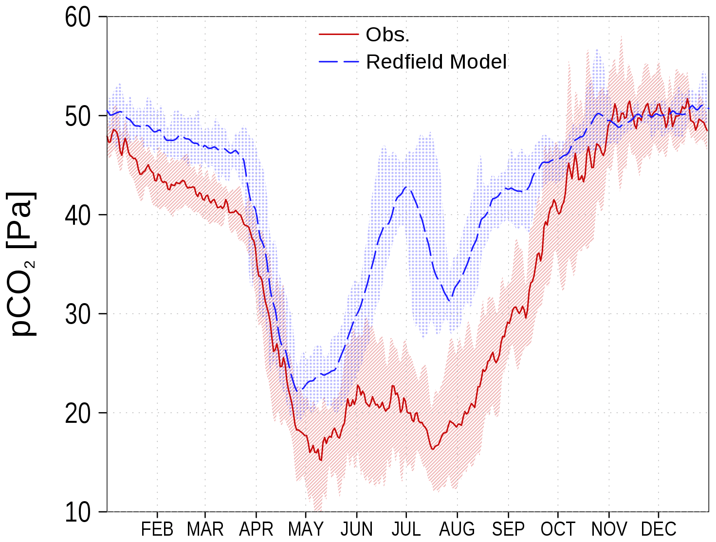
Figure 1spCO2 in the central Baltic Sea from a previous Redfield stoichiometry version of ERGOM (blue) and observations (red) as climatology (2003–2016) at station BY15 (Fig. 6). Shaded areas show the range between the 10th and 90th percentiles. Observations are available from SOCAT (see “Code and data availability”).
Fransner et al. (2018) demonstrated the considerable improvement by introducing non-Redfieldian dynamics which allow for an excess carbon uptake. Established methods for implementing a non-Redfieldian carbon fixation in ecosystem models are the cell quota model by Droop (1973) and/or additional carbon uptake due to the production of dissolved organic matter (DOM) (Fransner et al., 2018).
Several studies prove that the stoichiometry of healthy phytoplankton cells do not considerably deviate from the Redfield ratio. In an experimental setup for marine phytoplankton, Ho et al. (2003) showed that the biomass composition is generally close to the Redfield ratio. In situ data of particulate organic matter (POM) by Martiny et al. (2016) display only moderate deviations from the Redfield ratio. Considering that POM constitutes not only phytoplankton, other particles like heterotrophs or detritus may impact the observed ratios. With the aid of model experiments, Sharoni and Halevy (2020) showed that variations in POM stoichiometry are best explained by the taxonomic composition of phytoplankton compared to phenotypic plasticity, i.e., phytoplankton with a minimum flexibility of the nutrient cell quota, but a variation between adapted groups, best fits the observed elemental ratio variations on a global scale. Engel (2002) stated that “the fundamental need for N and P for biomass synthesis does not allow large deviations from Redfield”.
Dissolved organic matter in the ocean is one of Earth's major carbon reservoirs (Hansell et al., 2009). Many production, degradation, and consumption processes control its dynamics. An excellent review of DOM dynamics is given by Carlson and Hansell (2015). We will summarize some facts from this review which we think are important to guide our model development: the main producer of DOM is phytoplankton within the euphotic zone due to extracellular release (ER). Two common models exist to explain mechanisms for ER: (i) the overflow model and (ii) the passive diffusion model. The overflow model assumes an active DOM release by healthy cells. This process is directly coupled to primary production (PP) and regulates the frequently mismatching availability of irradiation and nutrients. The active ER will be used to dissipate energy from the photosynthetic machinery and protect it from damage. In the passive diffusion model, ER is controlled by different concentrations of DOM inside and outside of the cell. The concentration gradient forces an ER across the cell membrane. This process is more strongly coupled to phytoplankton biomass instead of PP. For both models, experimental evidence exists and it is possible that both are valid and, depending on environmental conditions, one or the other process is more active.
Although ER is coupled to PP in the overflow model, there is not a constant fraction of produced DOM. In fact, fractionation depends on nutrient availability and phytoplankton composition (Carlson et al., 1998). The ER of Phytoplankton consists of up to 80 % of carbohydrates which are important precursors for the formation of transparent exopolymer particles (TEPs). The TEPs are sticky and aggregate into larger particles which may sink down (Engel et al., 2004) and are methodically often counted as particulate organic carbon (POC) (Carlson and Hansell, 2015), therefore not considering TEP production results in underestimating ER (Wetz and Wheeler, 2007).
Considering the fact that biogeochemical models for the Baltic Sea with a Redfieldian carbon fixation are not able to reproduce the observed carbon cycle (see also Fig. 1) and a strong observational evidence for an ER of DOM (Hoikkala et al., 2015), we develop a model able to fix carbon beyond the classical Redfield ratio. In this study, we introduce a non-Redfieldian carbon uptake by maintaining the Redfield composition of living biomass, but allowing ER of highly carbon-enriched DOM in the model ERGOM 1.2 and show selected budgets derived from the model simulations.
2.1 Biogeochemical model
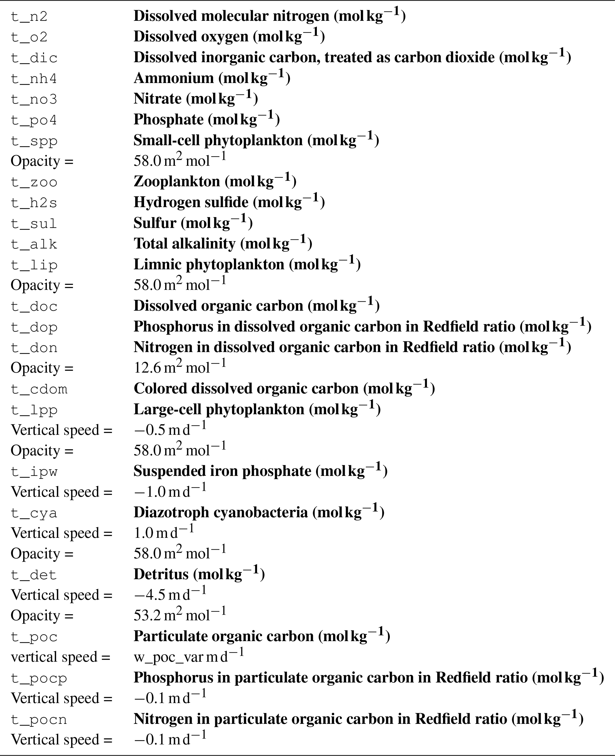
We start with explaining the biogeochemical model ERGOM (Leibniz Institute for Baltic Sea Research, 2015), which describes cycles of the elements nitrogen, phosphorus, carbon, oxygen, and partly sulfur.
Primary production (PP), forced by photosynthetically active radiation (PAR), is provided by three functional phytoplankton groups (large cells, small cells, and cyanobacteria). The chlorophyll concentration used in the optical model is estimated from the phytoplankton groups (Neumann et al., 2021). Dead particles accumulate in the detritus state variable. A bulk zooplankton grazes on phytoplankton and is the highest trophic level considered in the model. Phytoplankton and detritus can sink down in the water column and accumulate in a sediment layer. In both the water column and sediment, detritus is mineralized into dissolved inorganic nitrogen and phosphorus. Mineralization is controlled by water temperature and oxygen concentration. Oxygen is produced by primary production and consumed due to all other processes, e.g., metabolism and mineralization.
The stoichiometry in all organic carbon components of the model is confined to the classical Redfield ratio (Redfield et al., 1963). The advantage of this approach is the model's simplicity. However, observations of the carbon cycle in the Baltic Sea reveal the shortcomings of this kind of model (e.g., Fransner et al., 2018). Based on the findings presented in Sect. 1, specifically the underestimation of carbon fixation, we extended our model by introducing a non-Redfieldian stoichiometry into carbon fixation. The aim of this extension is to allow for carbon fixation beyond the part limited by the availability of nutrients.
Our basic idea is that the elemental composition in vegetative phytoplankton cells remains at the Redfield ratio and under certain circumstances, extracellular dissolved organic matter (DOM) is produced. This extracellular DOM has a fairly flexible elemental ratio. The produced DOM is subject to flocculation (TEP formation) with a certain rate and eventually sinks down as particulate organic matter (POM). In order to realize the elemental flexibility in DOM, we introduce three different DOM state variables together with the POM counterparts. We call the DOM state variables dissolved organic carbon (DOC), dissolved organic nitrogen (DON), and dissolved organic phosphorus (DOP). The model considers DOC as polysaccharides (COH2), and DON and DOP as DOC with additional nitrogen (N) and phosphorus (P), respectively. In DON and DOP, the elemental ratio is fixed to the Redfield ratio and they are counted in units of N and P: DON – and DOP – (COH2)106P. Altogether, model DOM has a flexible elemental ratio with the restriction that the carbon fraction is never below the Redfield ratio. That is, DOM is usually enriched by carbon compared to the Redfield ratio. One could also have used one DOM state variable with a completely free elemental ratio. However, we used the different DOM compartments because we may consider a different fate for DOC, DON, and DOP later.
The production of DOC, DON, and DOP by phytoplankton is controlled by light availability and nutrient concentrations. Under optimal conditions, primary production increases phytoplankton biomass. When nutrients become limiting, DOM production increases while the production of phytoplankton biomass decreases. A schematic is shown in Fig. 2. In the case of N limitation, DOP is produced and under P limitation, DON is produced. If both N and P become depleted, the fraction of produced DOC increases. We have to note that only phytoplankton is able to produce DOM. This means that if phytoplankton biomass decreases because a net growth is not possible due to e.g., nutrient limitation, the DOM production will decrease as well. In particular, the DOM production is controlled by a reversal of the phytoplankton nutrient limitation. Gross phytoplankton growth in our model is as follows:
where PY is the phytoplankton biomass, r0 the maximum uptake rate, and ln are limitation functions ranging between 0 and 1. Subscripts N, P, and L are for nitrogen, phosphorus, and light, respectively; lT is a (possible) temperature impact on uptake. For nutrient limitation (lN,lP), we use a squared Monod kinetics model (Monod, 1949; Neumann et al., 2002). Light limitation (lL) follows Steele (1962) and for temperature control (lT), a Q10 rule is applied (Eppley, 1972) meaning doubling of growth rates with a 10 K temperature increase. For the temporal development of the DOM compartments we formulate:

Figure 2Schematic of DOM production. In the case of sufficient nutrients nitrogen (N) and phosphorus (P), phytoplankton biomass is produced. If N becomes depleted, DOP is produced and if P is depleted, DON is produced. If both N and P are depleted, DOC is produced.
The dependence of nutrient uptake in relation to carbon uptake on nutrient concentrations is shown in Fig. 3. For this purpose, we divide the nutrient assimilation for nutrients N and P by the carbon assimilation. The assimilation consists of phytoplankton growth (Redfield ratio) and ER defined in Eq. (1) and Eqs. (2)–(4), respectively. The nutrient concentrations are normalized by the half saturation constant from the Monod kinetics. A value of 1 in Fig. 3 denotes a carbon uptake in the Redfield ratio, while smaller values indicate an excess carbon uptake. In the case of low N concentrations, the N:C uptake ratio declines to 0. The P:C uptake ratio in this case depends on P concentrations and asymptotically approaches 0.5 for high P concentrations, i.e., ER consists of DOC and DOP in equal shares. Figure 4 demonstrates the different carbon uptake rates with a realistic example from our model simulations for station BY15 (Fig. 6) in 2017. In spring, when nutrients are available in high concentrations, phytoplankton biomass production dominates. Later in spring, N becomes exhausted and the fraction of DOP production increases. The DOC production dominates in summer when both N and P are at low concentrations; DON production is always at a low level at this station because the winter concentration of P is in excess to the N concentration with respect to the Redfield ratio. Altogether, carbon fixation is solely mediated by phytoplankton. Depending on the nutrient concentrations, organic carbon production ends up in phytoplankton, DOC, DON, and DOP. The fractionation is controlled by the limitation functions which ensure a smooth transition and co-existence of the different carbon fixation pathways.

Figure 3Nutrient (N, P) to carbon uptake ratios as a function of nutrient concentrations. Nutrient concentrations are normalized by the half saturation constant in the limitation function and the uptake is normalized by the Redfield ratio. A ratio of 1 means uptake in the classical Redfield ratio and values less than 1 describe an excess carbon uptake.
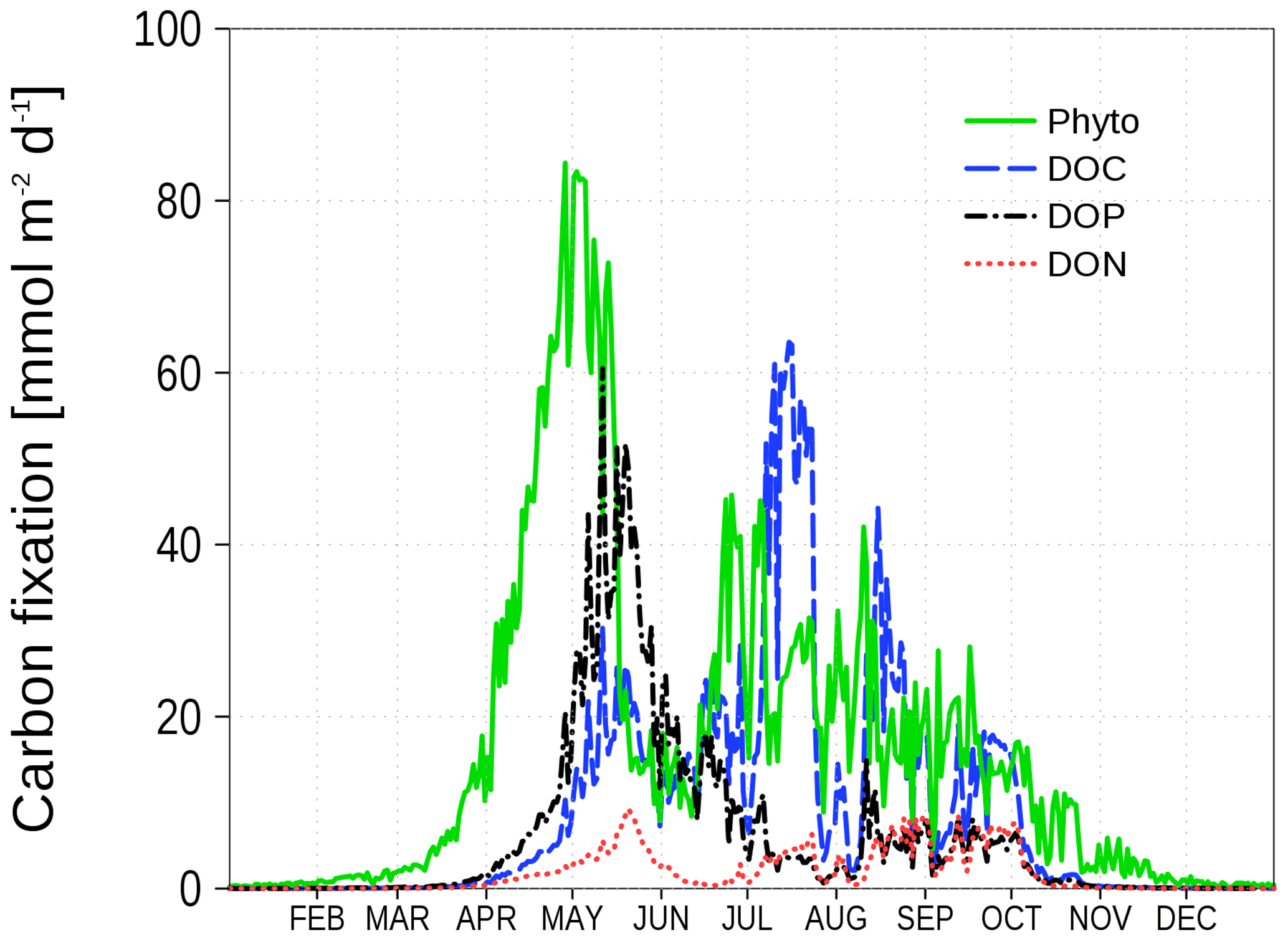
Figure 4Vertically integrated carbon uptake rates at station BY15 (Fig. 6) in 2017. Shown are production rates for different organic matter compartments: phytoplankton, DOC, DOP, and DON.
Extracellular DOM eventually forms particles (POC, PON, POP) which constitute transparent exopolymer particles (TEP). Engel (2002) shows a linear relation between dissolved inorganic carbon (DIC) uptake and TEP production, implying a direct transfer from DOM to TEP. Therefore, we chose a simple rate equation for DOC flocculation:
where rf is a constant rate for POC formation. The same equation applies for DON and DOP when forming their counterparts PON and POP.
For particle sinking, we apply a Martin curve (Martin et al., 1987) which means a linear increase of the sinking speed with depth:
where w is the sinking speed, a a constant, and z the depth. This approach is investigated by e.g., Kriest et al. (2012) and yields good results for the deep ocean. In the Baltic Sea application, we could improve the simulated oxygen concentrations by using the non-constant sinking speed.
A schematic of ERGOM is shown in Fig. 5. Ellipses denote state variables and rectangles processes. The complete set of equations is given in Appendix B.
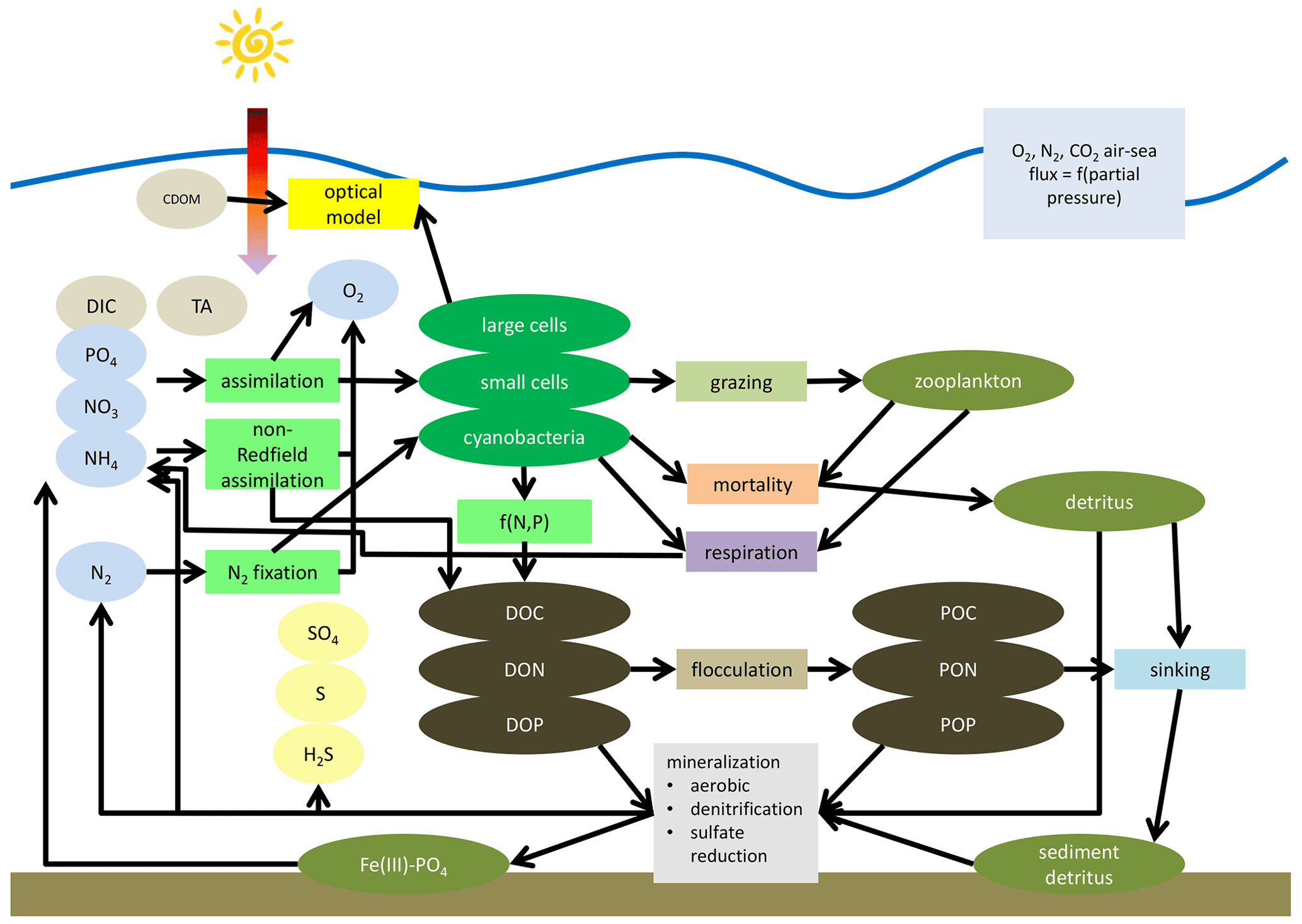
Figure 5Simplified schematic of the ERGOM model. State variables are shown as ellipses and processes as rectangles. State variables are explained in Table 1. Arrows show fluxes of elements mediated by processes. Not all arrows are shown for simplicity of the schematic, e.g., oxygen demanding processes do not show arrows from the oxygen state variable.

Figure 6Model domain and bathymetry used for this model study. Red dots denote stations to which we will refer later in the text. Bathymetry contour lines have a distance of 50 m. Boundaries of regions are in blue with Bay of Bothnia (BB), Bothnian Sea (BS), Gulf of Finland (GF), Gulf Of Riga (GF), and Baltic Proper (BP). The map was created using the software package GrADS 2.1.1.b0 (http://cola.gmu.edu/grads/, last access: 14 December 2021), using published bathymetry data (Seifert et al., 2008).
The relation between model state variables and observed dissolved organic carbon (DOCobs) in carbon units is as follows:
Taking into account that the model state variables DON and DOP are counted in nitrogen and phosphorus units (see Table 1), they correspond to the observed nitrogen and phosphorus in DOM. We have to note that our model DOM (DOC, DON, DOP) constitutes only the labile part of DOM existing in the Baltic Sea. Usually, the refractory DOM fraction, not considered in the model, is much larger than the labile fraction.
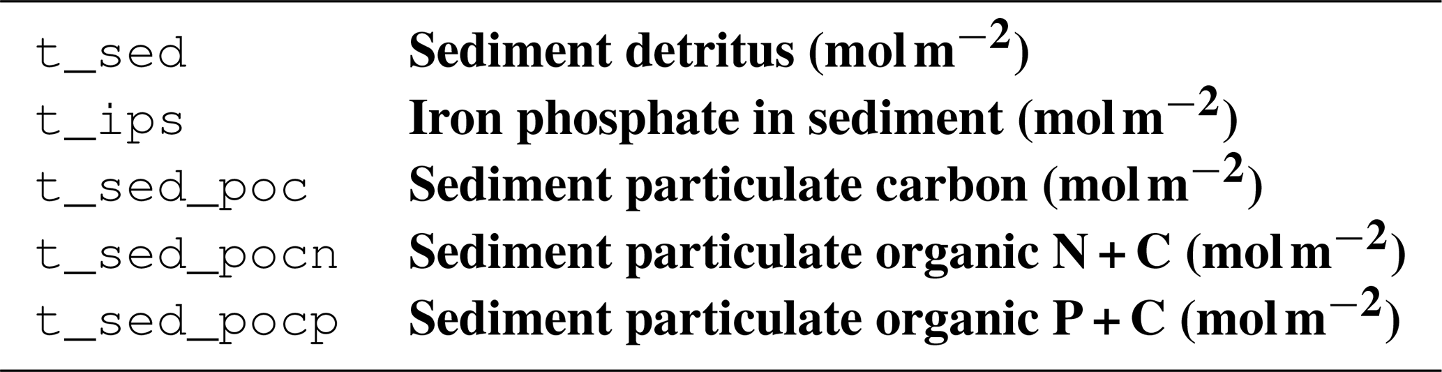
Table 1State variables of the biogeochemical model ERGOM shown in Fig. 5.
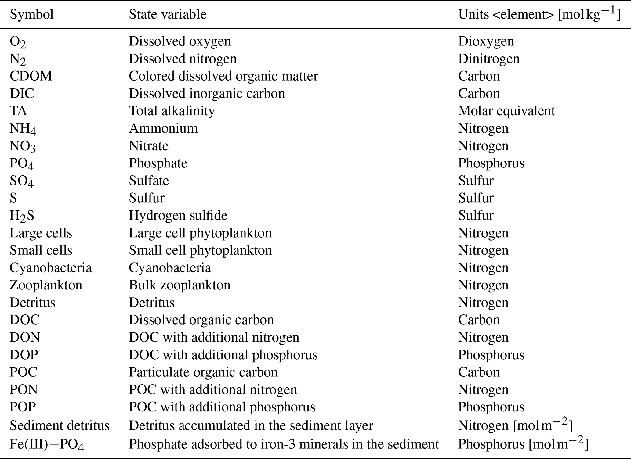
Sediment state variable units are mol m−2.
2.2 Rationale for model design
The model design was guided by the main principle of keeping the model as simple as possible. This is especially important for model applications in a 3D environment, at long timescales like climate change, and in ensemble approaches because we want to keep the computational effort at a feasible level. Therefore, we decided to implement ER which allows flexible nutrient to carbon uptake ratios. A cell quota approach was not implemented since it requires a number of additional state variables.
We do not doubt the flexibility in phytoplankton stoichiometry. However, from a modeler's point of view, we consider a fixed elemental ratio in phytoplankton as a reasonable simplification with the advantage of less model complexity. We proved this concept by the application for the Baltic Sea. Measurable state variables agree well with the model data (Appendix A). We achieved a considerable improvement, especially for spCO2. Improving the carbon cycle mass balances was the main focus of our model development since it plays a vital role in the energy cascade of the marine ecosystem.
For this reason, we decided to transfer the intracellular deviation from a fixed elemental ratio into DOM with a flexible ratio as ER. We justify this assumption by the small effect of intracellular flexibility on carbon uptake (see also Sect. 2.3) which is a focus of our model development. Furthermore, observations of ratios, which distinguish between living cells and POM, are still missing in the Baltic Sea area. In the following discussion, we review literature supporting our assumptions.
In Kuznetsov et al. (2011, 2008), we applied the Larsson et al. (2001) findings for diazotrophs. However, these elemental ratios do not explain observed spCO2, although the ratio in diazotrophs increases up to 4-fold and an additional, artificial spring-blooming species of diazotrophs was introduced. Larsson et al. (2001) did their study with filamentous cyanobacteria. Filaments consist not only of vegetative cells but also of akinetes, heterocysts, and vacuoles which together are not necessarily composed according the Redfield ratio. Vacuoles in particular develop in a later state of the bloom and may explain an increasing ratio. These mechanisms are not explicitly formulated in our model and parameterized instead by ER.
Nausch et al. (2009) showed that the elemental ratio (up to 400) is especially elevated in cyanobacteria (their Fig. 7) similar to Larsson et al. (2001). However, the ratio (100–200) in POM at the same station is much lower (same figure). Taking the high ratio of cyanobacteria into account, the ratio of the remaining POM is close to the Redfield ratio (∼100). In their Table 2, ratios in POM are given (7–9) which appear close to Redfield. The slight C enrichment in POM cannot explain the observed spCO2 (Kuznetsov et al., 2011).
Kreus et al. (2015) introduced extracellular release and cell quota into their model and run it in a 1D environment in the central Baltic Sea. Two experiments have been performed: (a) variable quotas and (b) fixed quotas. The POCPON ratios are virtually the same for both experiments while POCPOP ratios show a different seasonality. However, they conclude that fueling the summer cyanobacteria bloom controlling the carbon cycle and nitrogen dynamics is determined by DOM which is also part of our model. The shortcoming in the DIP cycle in experiment (b) of Kreus et al. (2015) has been solved with our approach. In summary, one can conclude that cell quotas do not have an impact on the nitrogen and carbon cycle (their Fig. 5).
2.3 Differences to earlier approaches
Omstedt et al. (2009) inferred that the carbon dynamics in the Baltic Sea cannot be correctly represented with a strict Redfield-based model. Since this time, several carbon cycle models have been proposed for the Baltic Sea. We will review a few of them and highlight the differences to our approach.
Kuznetsov et al. (2008, 2011) used an elevated ratio in cyanobacteria. However, they demonstrated that non-Redfieldian biomass, at least during summer since only cyanobacteria are considered, is by far not sufficient to reproduce the observed spCO2. We use also this result as an argument to focus on ER
Wan et al. (2011) changed the uptake and mineralization ratios but did not introduce a flexible elemental uptake ratio. This approach may violate the mass conservation.
Fransner et al. (2018) introduced both non-Redfieldian phytoplankton biomass and the ER of DOC. They found that for the Gulf of Bothnia, “A substantial part of the fixed carbon is directly exuded as semilabile extracellular DOC” (26 %–52 %). Their study is limited to the northern Baltic. Therefore, it has not been shown that the model works reasonably for the whole Baltic Sea. Unfortunately, the authors do not show any deep-water properties like oxygen which may be impacted by the increased downward carbon flux.
The model used in Kreus et al. (2015) was applied at a station in the central Baltic Sea. Thus, it is not shown that the model gives reasonable results in a 3D environment. It uses a similar approach as in Fransner et al. (2018) with a flexible elemental ratio in phytoplankton and ER of DOM. From our point of view, it involves the disadvantage of enhanced computational effort but does not prove that cell quotas improve the carbon cycle dynamics (Sect. 2.2).
2.4 Model setup and simulations
For model testing, we use a coupled system of circulation and biogeochemical models similar to that in Neumann et al. (2021). The circulation model is MOM5.1 (Griffies, 2004) adapted for the Baltic Sea. The horizontal resolution is 3 nautical miles. Vertically, the model is resolved into 152 layers with a layer thickness of 0.5 m at the surface and gradually increasing with depth up to 2 m. The circulation model is coupled with a sea-ice model (Winton, 2000) accounting for ice formation and drift. The biogeochemical model ERGOM, described in Sect. 2.1, is coupled with the circulation model via the tracer module which is part of the MOM5.1 code.
The code for the biogeochemical model is generated automatically. Fundamentals are a set of text files describing the biogeochemistry independent of programming language and the host system. Code templates describe physical and numerical aspects and are specific for a certain host, e.g., a circulation model. All the necessary ingredients (the code generation tool, text files, and templates for several systems) can be downloaded from Leibniz Institute for Baltic Sea Research (2015). The same technique is used e.g., in Neumann et al. (2021).
We run the model for about 70 years (1948–2019) after a spin-up of 50 years. The long simulation time allows us to assess the model performance under different forcing conditions, e.g., as the eutrophication of the Baltic Sea in the 1970s and the nutrient load reduction beginning in 1990.
2.5 Data
The model has been forced by meteorological data from the coastDat-2 dataset (Geyer and Rockel, 2013). Nutrient loads to the Baltic Sea due to riverine discharge and atmospheric deposition have been compiled based on data from HELCOM assessments (HELCOM, 2018, e.g.,). Riverine alkalinity follows data provided in Hjalmarsson et al. (2008). In Table 2, we compare riverine alkalinity concentration and loads with published data from Hjalmarsson et al. (2008) and Gustafsson et al. (2014b). The data are relatively similar with the exception of the Baltic Proper. Gustafsson et al. (2014b) use considerably lower values, which impact the total load. Our mean concentrations differ slightly from Hjalmarsson et al. (2008). We used the basin-wide and constant concentration values given in Hjalmarsson et al. (2008) and assigned the data to our model rivers which show interannual runoff variability. This results in mean concentration deviations. Loads given in Table 2 result from runoff- and river-specific concentrations.
Table 2Average alkalinity concentration and loads in runoff for different basins in the Baltic Sea and from different authors. BP: Baltic Proper, GR: Gulf of Riga, GF: Gulf of Finland, BS: Bothnian Sea, BB: Bay of Bothnia (Fig. 6). HS: Hjalmarsson et al. (2008), GS: Gustafsson et al. (2014b), NM: this study.
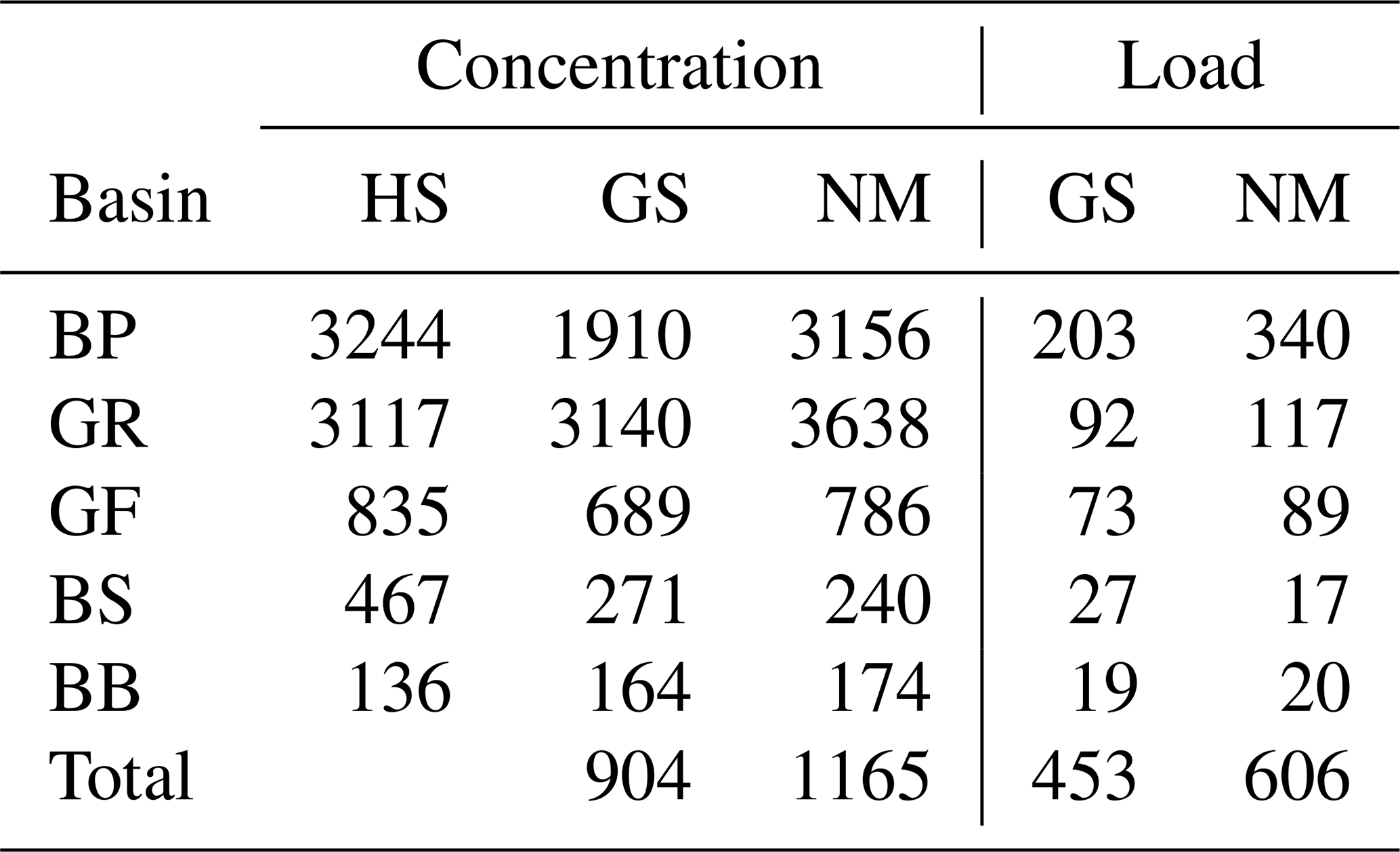
Alkalinity concentration in µmol kg−1 and loads in Gmol a−1.
The spCO2 for model validation have been extracted from the SOCAT (Surface Ocean CO2 Atlas) database (https://www.socat.info/, last access: 15 November 2022). The majority of data are from the voluntary observing ship (VOS) Finnmaid between Lübeck-Travemünde and Helsinki. The VOS Finnmaid is a component of the European ICOS (Integrated Carbon Observation System) research infrastructure. Data processing and quality control follow the SOCAT guidelines (Bakker et al., 2016; Pfeil et al., 2013). Additional observation data used for comparison with model results are available from public databases. Details are given in the “Code and data availability” section.
3.1 How the non-Redfieldian approach works
In this section, we demonstrate how a non-Redfieldian elemental ratio in organic matter (OM) develops due to the model extensions described above. Organic matter involves all forms of model DOM and POM including model phytoplankton, zooplankton, and detritus. We show data averaged over the whole simulation period and seasonal climatologies. The elemental ratios are based on molar concentrations.
In Figs. 7 and 8, the carbon (C) to nitrogen (N) and carbon to phosphorus (P) ratios in organic matter from surface water are shown. In both figures, the elemental ratios are normalized so that a ratio of 1 is for the classical Redfield ratio. The figures highlight the different nutrient-limitation provinces in the Baltic Sea. The C:N ratio is high in the central Baltic Sea where N is a limiting nutrient and consequently the C:P ratio is low. The opposite is true in the northern Baltic Sea where P is the limiting nutrient. We have to note that our model approach does not allow for C:N and C:P ratios below Redfield ratios in the DOM and POM fractions. Hence, the elemental ratios in OM are always above 1. River mouths are the exception; here almost no nutrient limitation keeps the C:N and C:P ratios close to 1.
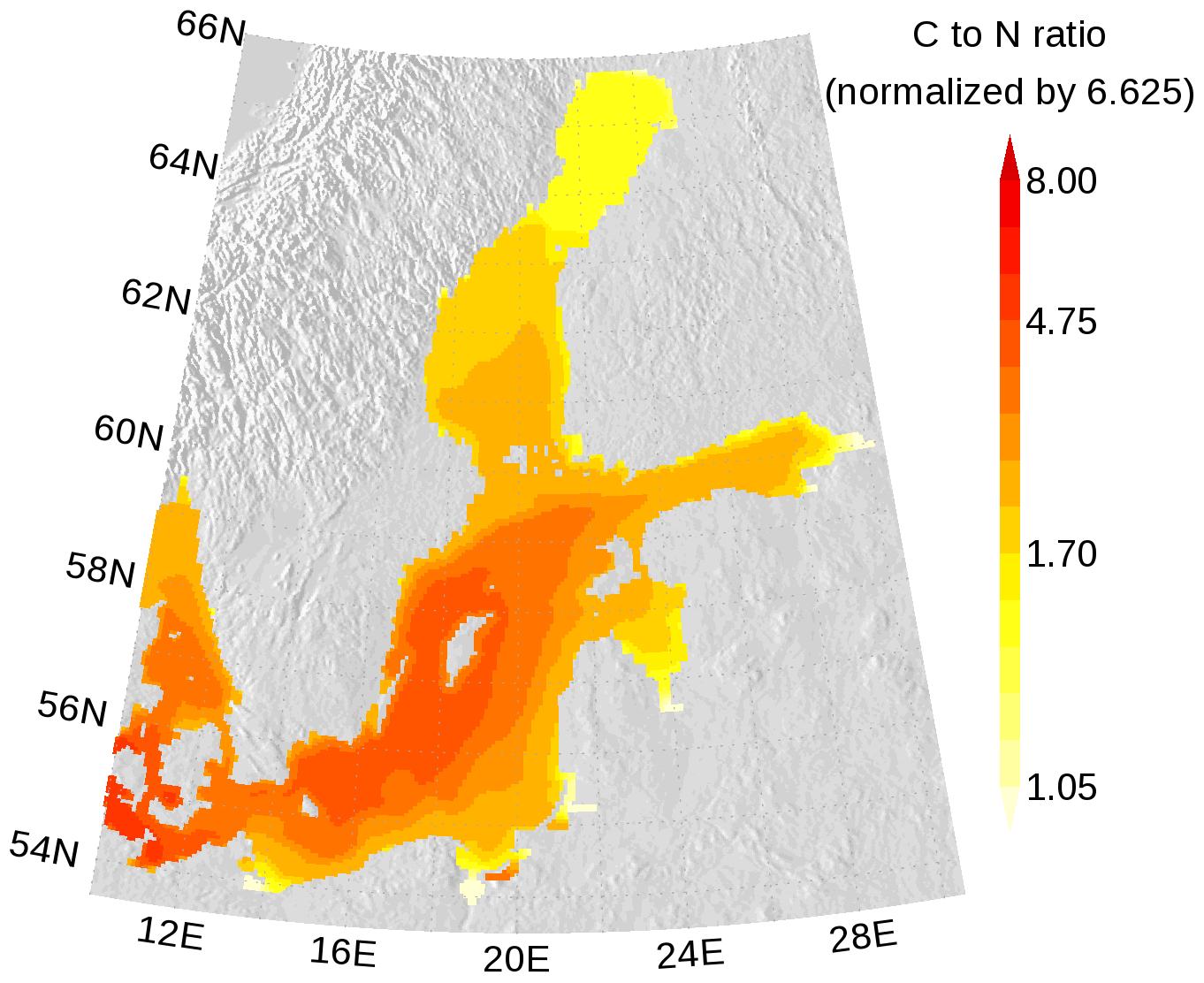
Figure 7Annual mean elemental carbon (C) to nitrogen (N) ratio in surface organic matter. The ratio is normalized and a ratio of 1 refers to the classical Redfield ratio. The map was created using the software package GrADS 2.1.1.b0 (http://cola.gmu.edu/grads/, last access: 14 December 2021), using published topography data (Seifert et al., 2008).
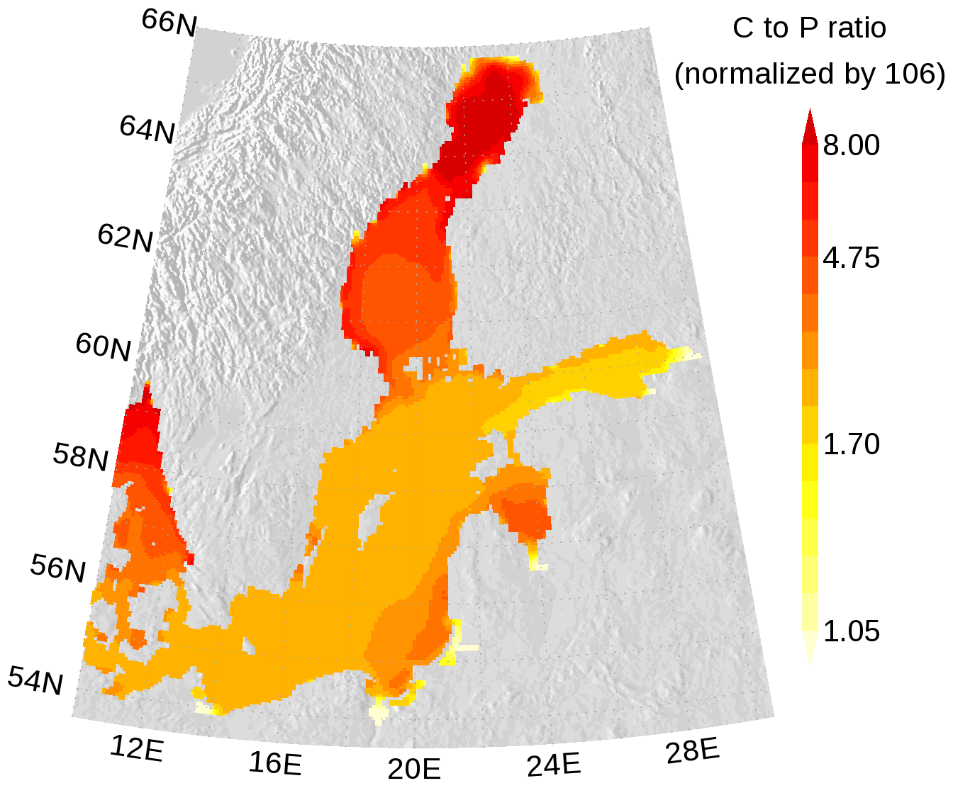
Figure 8Annual mean elemental carbon (C) to phosphorus (P) ratio in surface organic matter. The ratio is normalized and a ratio of 1 refers to the classical Redfield ratio. The map was created using the software package GrADS 2.1.1.b0 (http://cola.gmu.edu/grads/, last access: 14 December 2021), using published topography data (Seifert et al., 2008).
We show the N:P ratio in OM and its seasonality in Fig. 9. Again, the figure shows the separation between the nutrient-limitation provinces. A low N:P ratio denotes N limitation in the central Baltic Sea and a high N:P ratio shows P limitation in the northern Baltic Sea. During the course of the year, the N:P ratio in the central Baltic Sea increases due to nitrogen fixation by cyanobacteria. The temporal development of the DOM fractions can be seen in Fig. 10. In the N-limited Gotland Basin (Fig. 10a), surplus phosphate is transferred into DOP after depleted N starts limiting phytoplankton growth. With intensified nutrient limitation DON and DOC will also be produced by phytoplankton. In summer, with a higher demand of phosphorus by cyanobacteria, the DOP pool is depleted. Contrastingly, in the Bothnian Bay, the northern part of the Baltic Sea, surplus nitrogen is transferred into DON (Fig. 10b). Almost no DOP develops. In Fig. 11, we show the surface climatology of simulated DOCobs (Eq. 7) at station BY15 together with observations. Observed DOC concentrations constitute refractory fractions to a large extent. In contrast, in the model we only consider the labile, autochthonous part of DOC. Therefore, we subtracted 305 µmol kg−1 from the observations which is the mean winter concentration. The annual DOC cycle in the observed data appears less pronounced compared to the modeled DOCobs cycle.
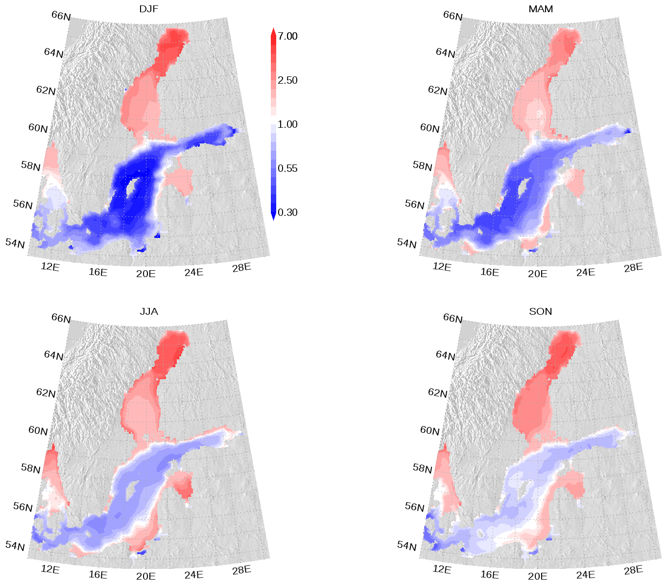
Figure 9Seasonal mean elemental nitrogen (N) to phosphorus (P) ratio climatology in surface organic matter. The ratio is normalized and a ratio of 1 refers to the classical Redfield ratio. The map was created using the software package GrADS 2.1.1.b0 (http://cola.gmu.edu/grads/, last access: 14 December 2021), using published topography data (Seifert et al., 2008).
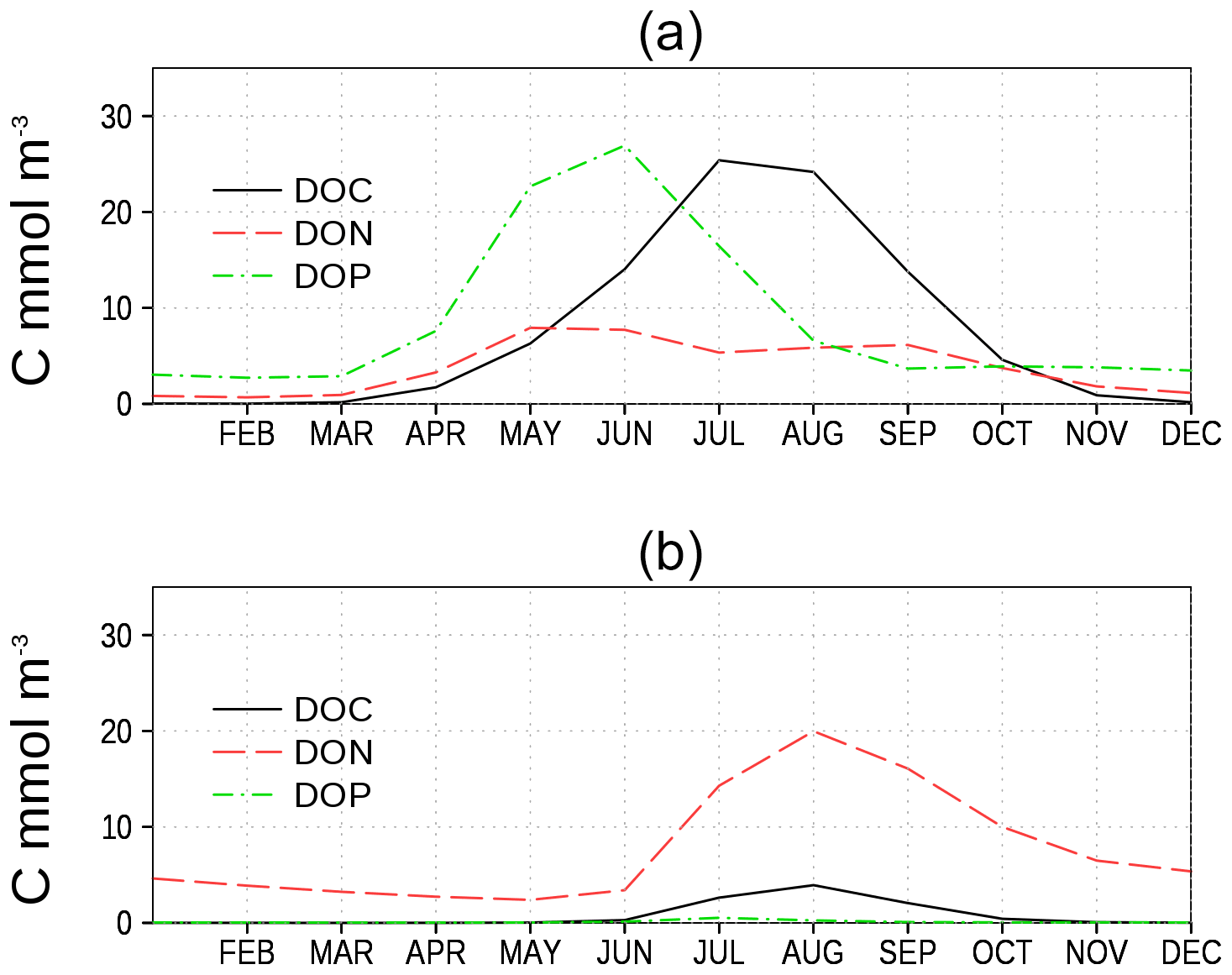
Figure 10Climatology of surface model DOC, DON, and DOP (in carbon units, Table 1 and Eq. 7) at two stations. (a) Central station in the eastern Gotland Basin (BY15), and (b) central station in the Bothnian Bay (BoB, Fig. 6). Model DON and DOP are converted into carbon units to show all variables on a comparable level.
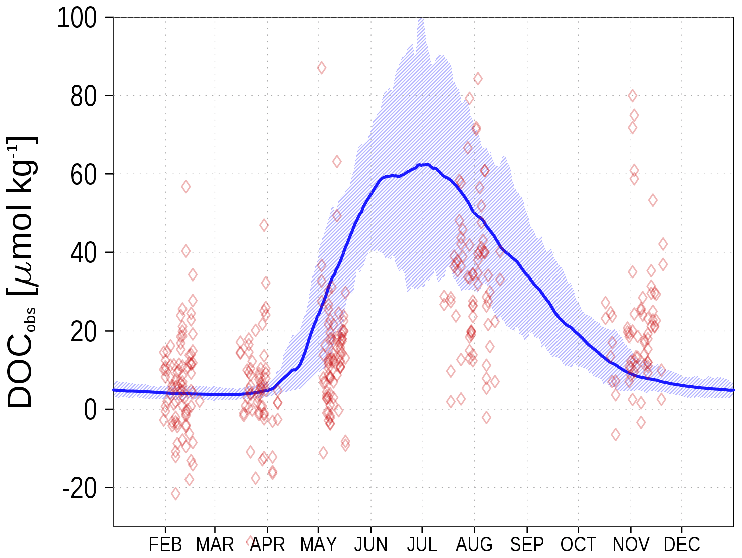
Figure 11Climatology (1995–2019) of simulated surface DOCobs (Eq. 7) at station BY15 (blue line) and observed DOC (red diamonds). The diamond's opacity reflects the frequency of observations. The shaded area shows the range between the 10th and 90th percentiles. From observations, 305 µmol kg−1 have been subtracted. Observed DOC data are available from the IOW ODIN database (see “Code and data availability” section).
3.2 Primary production and extracellular production
We consider primary production (PP) as the carbon fixation contributing to phytoplankton biomass while extracellular production (EP) is the carbon fixation resulting in DOM (DOC, DON, and DOP state variables). Figure 12 shows the time series and climatology of PP and EP as means of the whole model domain. Carbon fixation is dominated by EP. With increasing nutrient availability beginning in the 1960s, the fraction of PP increases (Fig. 12a). The PP and EP climatology in Fig. 12b shows that PP dominates in spring and fall, and EP dominates in summer. Figure 12c shows the PP of the model phytoplankton groups. Most PP occurs in spring, mediated by the large-cell phytoplankton group LPP. In contrast, most EP is mediated by the small-cell phytoplankton group SPP in summer (Fig. 12d).
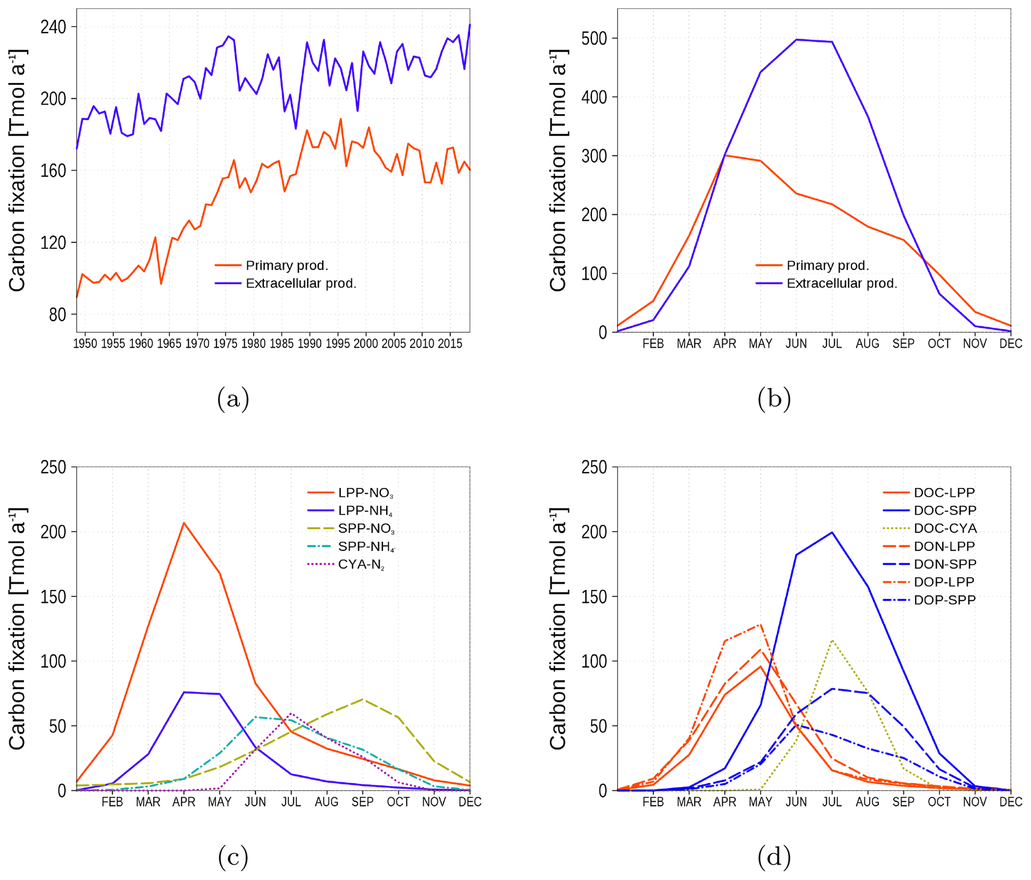
Figure 12Temporal and spatial mean primary and extracellular carbon fixation by model phytoplankton. (a) Time series of annual carbon fixation. (b) Climatology of carbon fixation. (c) Climatology of primary production related to different uptake processes. LPP-NO3 and LPP-NH4: carbon fixation by the large-cell phytoplankton group related to NO3 and NH4 uptake, respectively. SPP-NO3 and SPP-NH4: the same as for LPP, but for the small-cell phytoplankton group. CYA-N: Carbon fixation by cyanobacteria related to nitrogen fixation. (d) Climatology of extracellular production related to different phytoplankton groups: red lines are uptake by LPP, blue lines by SPP, and green line by cyanobacteria. Different line styles refer to DOC, DON, and DOP. All model variables have been converted into carbon units (Eq. 7).
3.3 Assessment of biogeochemical variables
We especially show model data and observations for sea surface carbon dioxide pressure and alkalinity. Other biogeochemical variables are shown in Appendix A.
3.3.1 Sea surface pressure of carbon dioxide (spCO2)
One motivation to introduce a non-Redfieldian carbon fixation into the ecosystem model ERGOM was the mismatch in observed and simulated spCO2 (Kuznetsov et al., 2011, see also Fig. 1). Redfield models are not able to explain the low observed spCO2 during summer. Temperature increase and ongoing mineralization in the surface layer increase the spCO2 to unrealistic values in the simulations. One conclusion was that a substantial carbon fixation still continues after nutrient limitation. Consequently, the carbon fixation is not restricted to the classical Redfield ratio.
For the spCO2 benchmark, we use data taken underway from the voluntary observing ship (VOS) Finnmaid regularly traveling between Lübeck-Travemünde and Helsinki. For more details, see Sect. 2.5 and Schneider and Müller (2018). The pathway and spCO2 observations taken by VOS Finnmaid and used in this study are shown in Fig. 13. From the regions denoted by green rectangles, we have selected data to compare with our model simulation. As can be seen from the pathway's opacity, region f was crossed less frequently than the other regions. The spCO2 climatology is shown in Fig. 14. The non-Redfieldian carbon fixation keeps the spCO2 low during summer as seen in the observations. In the northern regions c and e, the spring bloom seems to be delayed in the model. However, the general picture is a strongly improved spCO2 in the model compared to earlier model versions (e.g., Kuznetsov et al., 2011), as can be seen by comparing it to Fig. 1.

Figure 13spCO2 observations by VOS Finnmaid between 2003 and 2018 used for model analysis (red line). Opacity refers to frequency of observations. The green rectangles (a–f) denote regions selected for comparison with model data. The map was created using the software package GrADS 2.1.1.b0 (http://cola.gmu.edu/grads/, last access: 14 December 2021), using published topography data (Seifert et al., 2008).
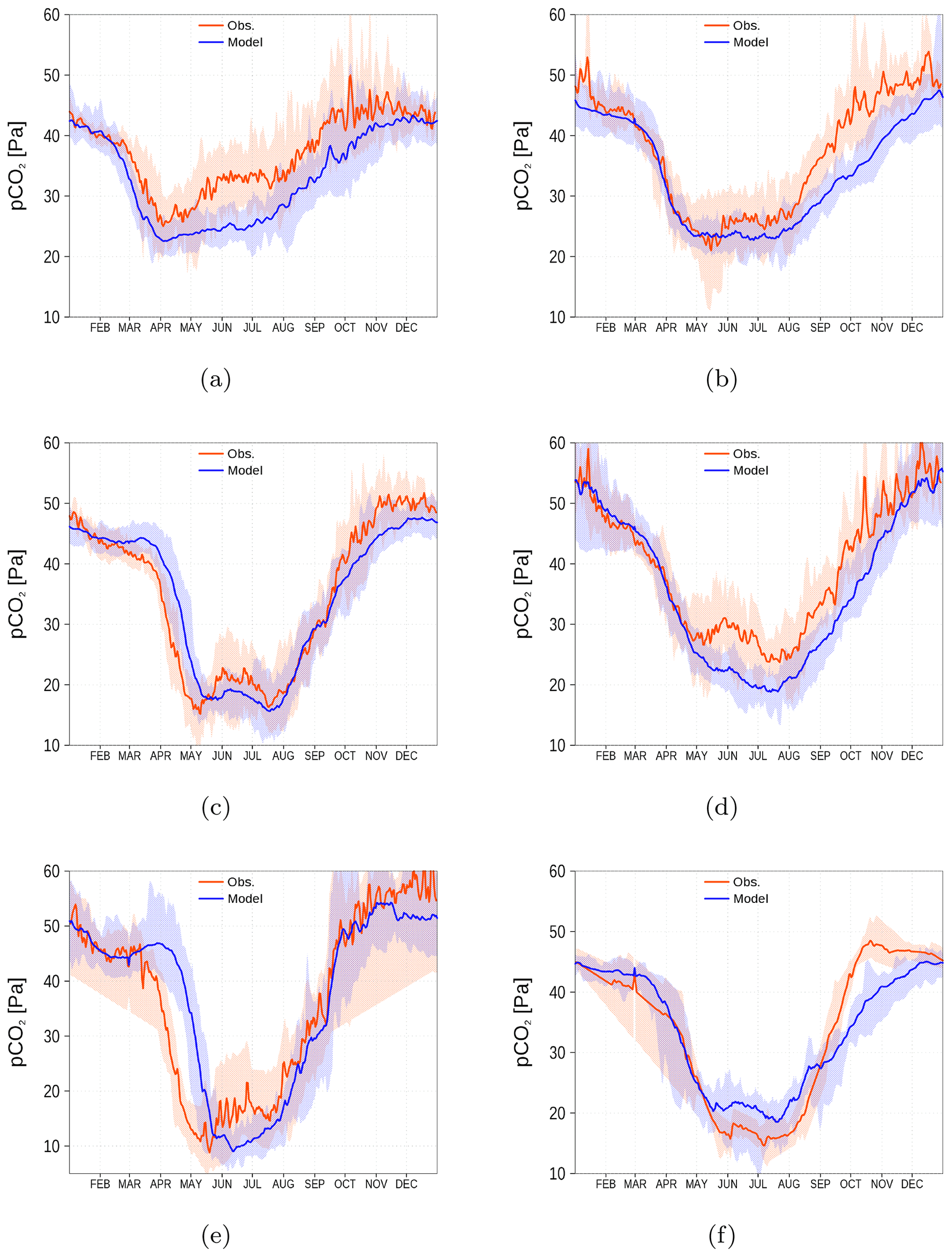
Figure 14spCO2 climatology (2003–2018) from observations (red) and model simulation (blue). Shaded areas show the range between the 10th and 90th percentiles. The subfigures (a–f) refer to the corresponding regions shown in Fig. 13 by green rectangles (a–f). Observations are available from SOCAT (see “Code and data availability” section).
3.3.2 Alkalinity
Alkalinity in the model is estimated after the equation for t_alk in Appendix B4.
Figure 15 shows the surface alkalinity climatology from observations (red diamonds) and the model simulation (blue). We show the climatology for six stations from the Kattegat (a) to the Bothnian Bay (f). While in the Kattegat, the simulated alkalinity reflects observations reasonably well, the model's underestimation amounts to roughly 20 % in the central Baltic Sea and increases further towards the northern Baltic Sea. This will also have an effect on the dissolved inorganic carbon (DIC) content. However, once in a quasi-equilibrium with the atmosphere, the air–sea fluxes will be affected only marginally.
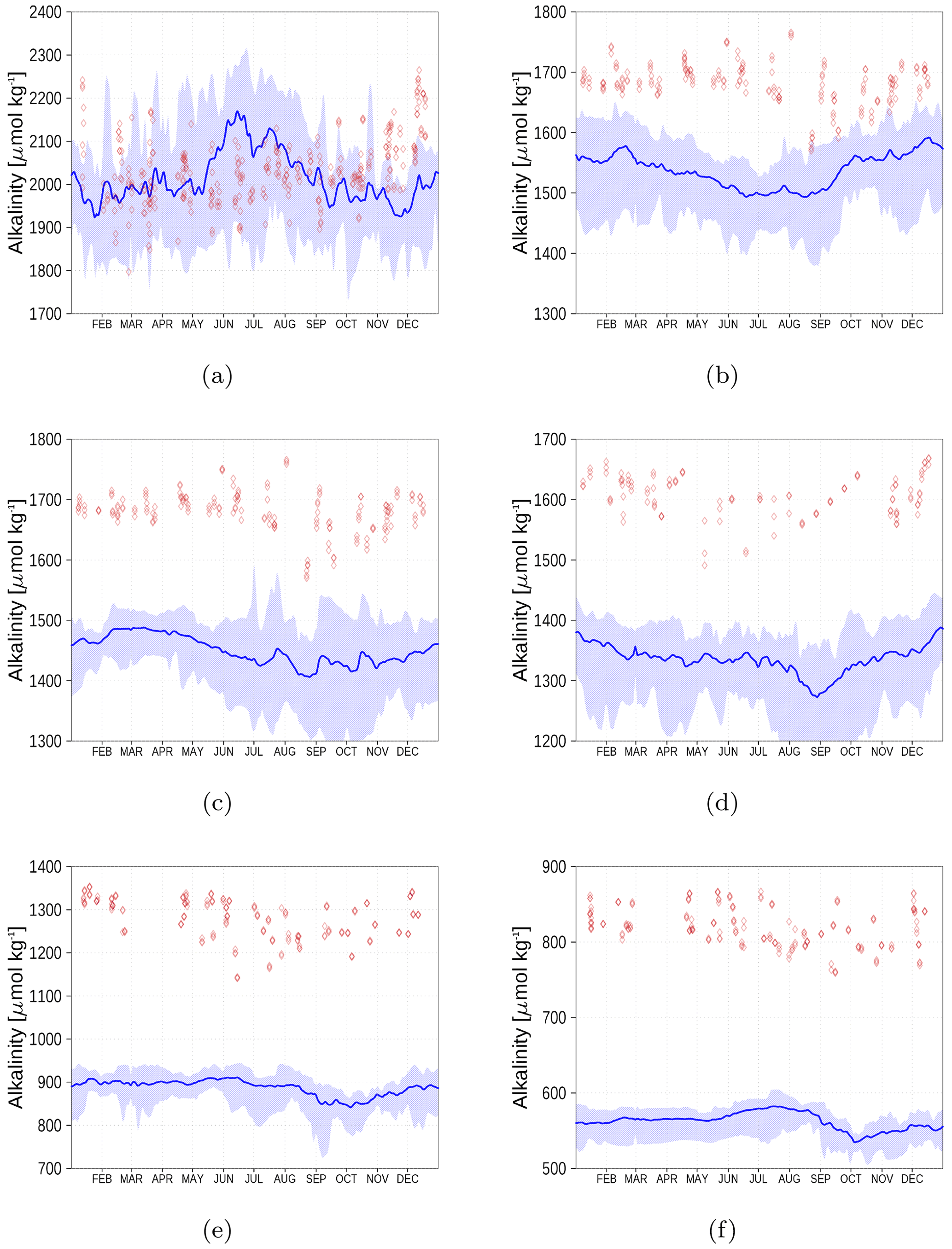
Figure 15Surface alkalinity climatology (2013–2018) from observations (red) and model simulation (blue). Shaded areas show the range between the 10th and 90th percentiles. The subfigures represent stations AH (a), BY1 (b), BY15 (c), BY31 (d), C3 (e), and F9 (f) (Fig. 6). Observed alkalinity data are available from the SHARK database (see “Code and data availability” section).
3.3.3 Nutrients
Nutrient surface concentrations are shown in Appendix A1. We have chosen six stations and regions to cover the whole Baltic Sea. Figures A1–A6 show the climatology and time series of simulated nitrate and phosphate together with observations. We find a good model performance for the western Baltic Sea, the central Baltic Sea, and the Gulf of Finland. In the northern Baltic Sea, the Gulf of Bothnia, the model slightly overestimates the nutrient concentrations. Nevertheless, the strong phosphate limitation in this region is well covered.
3.3.4 Oxygen
Oxygen concentrations of the near bottom water are shown in Appendix A2. Simulated concentrations are lower compared to observations, especially in the northern Baltic Sea.
3.4 Budgets
In this section, we show selected budgets as estimated from the model simulation and demonstrate that the model closes the budget.
3.4.1 Carbon budget
The carbon budget is shown in Fig. 16. The budget considers the inventory change in all carbon containing state variables in both the water column and sediment. Changes are the result of the boundary fluxes, riverine load, air–sea fluxes, transport from and to the North Sea, and burial of carbon in the sediment. The closed budget, which we show with the yellow line, should be 0, a deviation reflects cumulated numerical inaccuracies that are obviously small compared to the simulated signals. In Fig. 16a, annual fluxes and inventory changes are shown. Highest fluxes are the carbon export towards the North Sea and riverine carbon loads followed by air–sea fluxes and burial. Figure 16b and c show cumulated fluxes and inventory changes. Inventory changes are very small compared to the boundary fluxes. Therefore, in Fig. 16c, we show the inventory changes separately. The sediment inventory stays relatively constant. In the water column, carbon inventory increases in response to higher nutrient loads during the 1960s and 1970s (loads shown in Figs. 18 and 19).

Figure 16Model-domain integrated carbon budget. Shown are riverine loads, air–sea flux, burial, transport from the North Sea, and changes in the inventory of the ocean (water column) and the sediment. (a) Fluxes and inventory changes, (b) cumulated fluxes, and (c) a detailed view of the cumulated inventory changes in the ocean and sediment. The yellow line is the sum of all fluxes and inventory changes; it should be 0 in a closed budget. Note: We use a negative sign for sinks (burial and export towards North Sea).
3.4.2 Alkalinity budget
The alkalinity budget is shown in Fig. 17. The budget considers the inventory change in the alkalinity state variable in the water column. Changes are the result of the boundary fluxes, riverine load, and transport from and to the North Sea. In contrast to the carbon budget, the alkalinity budget is not closed (yellow line and Fig. 17c). The increasing sum of boundary fluxes and inventory changes, which should cancel each other out in a closed budget, suggests an internal alkalinity source. According to the implemented processes affecting alkalinity (Eq. for t_alk in B4), we attribute the alkalinity generation mainly to denitrification. The alkalinity generation is estimated to be roughly 7 % of the loads.
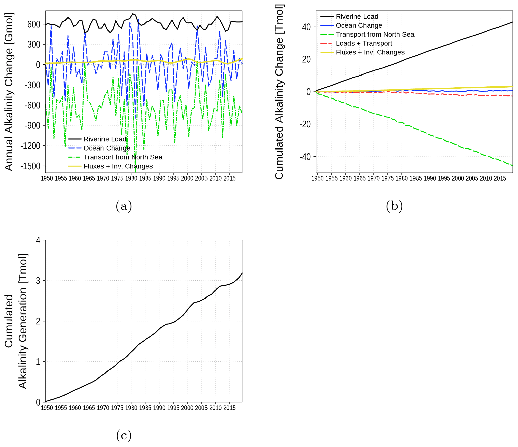
Figure 17Model-domain integrated alkalinity budget. Shown are riverine loads, transport from the North Sea, and changes in the inventory of the ocean. (a) Fluxes and inventory changes, (b) cumulated fluxes and inventory changes, and (c) residual of the budget which can be attributed to alkalinity generation. The yellow line is the sum of all fluxes and inventory changes and should be 0 in a closed budget. Note: We use a negative sign for sinks (export towards North Sea).
3.4.3 Nitrogen budget
The nitrogen budget is shown in Fig. 18 with inventory changes, boundary fluxes, loads, transport from and to the North Sea, burial in the sediment, and the internal sinks (denitrification) and sources (nitrogen fixation by cyanobacteria). The nitrogen load involves riverine, atmospheric, and point-source loads. The strongest fluxes are due to loads as a nitrogen source and sediment denitrification as a nitrogen sink. A detailed view of cumulated fluxes in Fig. 18c demonstrates that nitrogen fixation is nearly balanced by denitrification in the water column and only a small amount of nitrogen is exported towards the North Sea.
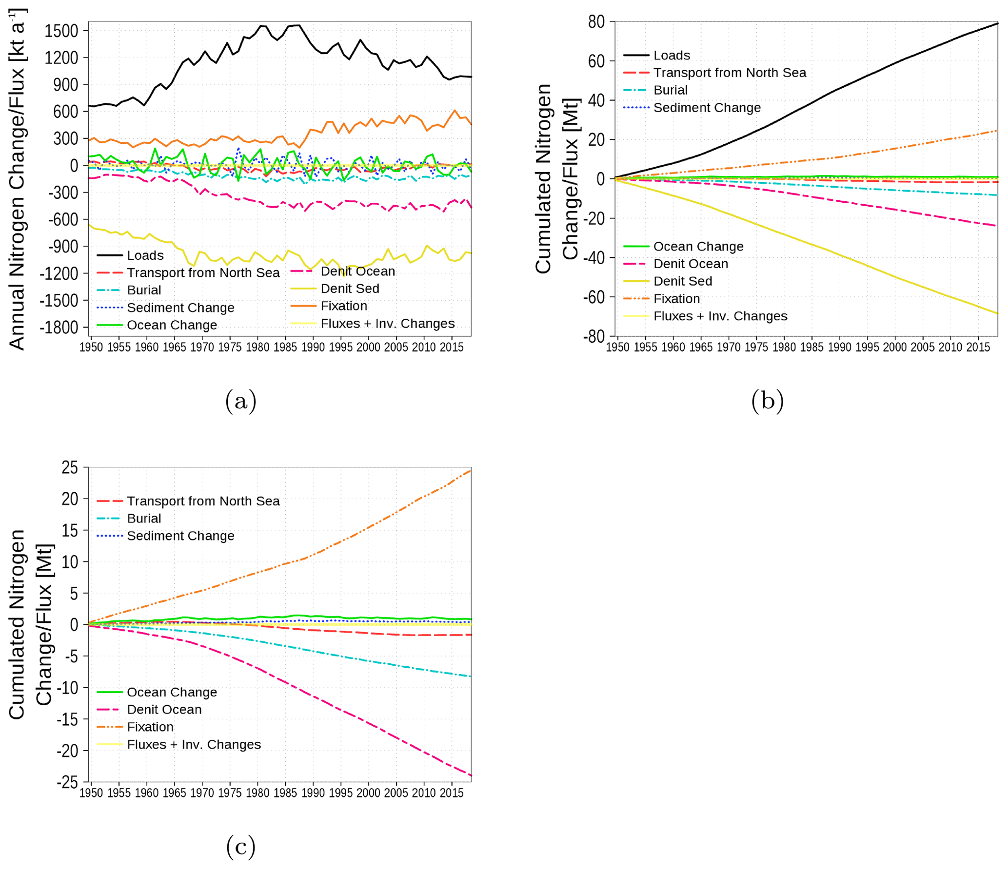
Figure 18Model-domain integrated nitrogen budget. Shown are loads (riverine, atmospheric, point sources), transport from the North Sea, burial, changes in the inventory of ocean and sediment, denitrification in sediment and ocean, and nitrogen fixation. (a) Fluxes and inventory changes, (b) cumulated fluxes and inventory changes, and (c) a detailed view without loads and sediment denitrification. The light yellow line is the sum of all fluxes and inventory changes and should be 0 in a closed budget. Note: We use a negative sign for sinks (burial, denitrification, and export towards North Sea).
3.4.4 Phosphorus budget
The phosphorus budget in Fig. 19 shows inventory changes, boundary fluxes, loads, transport from and to the North Sea, and burial. The phosphorus load involves riverine, atmospheric, and point-source loads. In contrast to nitrogen, no internal sinks and sources exist. The most important sink for phosphorus loads is the burial in the sediment. Similar to nitrogen, a small amount of phosphorus is exported towards the North Sea.
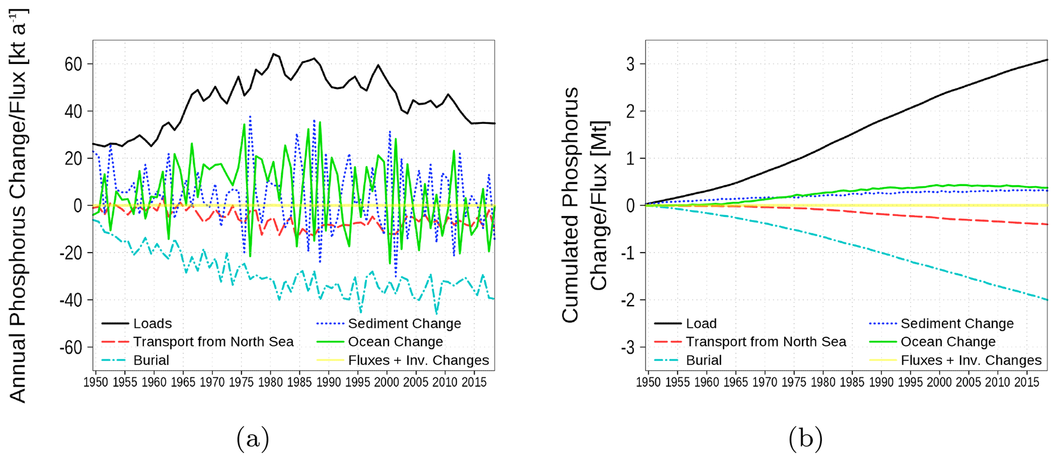
Figure 19Model-domain integrated phosphorus budget. Shown are loads (riverine, atmospheric, point sources), transport from the North Sea, burial in the sediment, and changes in the inventory of ocean and sediment. (a) Fluxes and inventory changes; (b) cumulated fluxes and inventory changes. The light yellow line is the sum of all fluxes and should be 0 in a closed budget. Note: We use a negative sign for sinks (burial and export towards North Sea).
We present a biogeochemical model for the Baltic Sea which is able to reproduce observed spCO2 data. This could be achieved solely by implementing a non-Redfieldian stoichiometry in carbon fixation. We realize this by introducing ER due to PP. Extracellular release results in DOM with a flexible elemental ratio and eventually flocculates into POM which sinks down. This approach reproduces observed spCO2, nutrients, and oxygen concentrations reasonably well for the whole Baltic Sea. A different approach is used by Fransner et al. (2018). In their model, in addition to a release of DOC, phytoplankton is formulated as a quota model, i.e., within the phytoplankton cells, a certain flexibility of the elemental ratio is allowed. This model is applied for the northern part of the Baltic Sea and reproduces spCO2 and surface nutrient concentrations well. The main difference between the models is the quota approach in Fransner et al. (2018), while in our model, uptake variations are directly transferred into ER. However, we have chosen the fixed ratio (Redfield ratio) in healthy phytoplankton cells because of some evidence from literature (Sect. 1) and less computational effort. We are also convinced that our approach is simpler to handle with respect to higher trophic levels which can rely on a fixed stoichiometry.
A similar model was introduced by Gustafsson et al. (2014a) who also uses the ER process to increase carbon fixation beyond the Redfield ratio. However, the authors do not show the model's performance with respect to spCO2 which might be due to missing or rare observations during this time. Macias et al. (2019) implemented a non-Redfieldian nutrient uptake in an ecosystem model for the Mediterranean Sea which results in a flexible elemental ratio in phytoplankton. This model gives good results for nutrients N and P but does not consider C. A cell quota model for global Earth system models is proposed by Pahlow et al. (2020) and Chien et al. (2020). This model also shows an advantage over fixed elemental ratio models with respect to nutrient concentration. However, proof against variables of the carbon cycle is unfortunately missing.
First evaluations of the simulation show an alkalinity generation of about 50 Gmol a−1 (Fig. 17). Gustafsson et al. (2014b, 2019) estimated an alkalinity generation of 84 and 120 Gmol a−1, respectively. Riverine alkalinity loads in our model are 600 Gmol a−1 and higher compared to loads in Gustafsson et al. (2014b, 2019) (470 Gmol a−1, Table 2). Altogether, both models underestimate the alkalinity concentration (Fig. 15) and consequently, sources of alkalinity are missing or underrepresented. Gustafsson et al. (2014b) investigated the contribution of a final pyrite burial in sediments to the missing alkalinity source with an advanced sediment model. However, pyrite burial can explain the missing source only partly. It still remains an open question whether riverine alkalinity loads are underestimated or an unknown source exists, e.g., groundwater discharge.
The Baltic Sea acts as a sink for carbon due to uptake of atmospheric carbon dioxide. The additional carbon is partly buried and the remaining fraction is exported towards the North Sea (Fig. 16). However, the northern Baltic Sea emits carbon dioxide into the atmosphere. Figure 20 shows the horizontal pattern of the mean atmosphere–ocean flux. Sources of carbon dioxide for the atmosphere are the northern Baltic Sea and upwelling regions. The latter are caused by prevailing westerly winds with upwelling near the Swedish coast and in the Gulf of Finland. The upwelled, CO2-rich deep water eventually comes into contact with the atmosphere and equilibrates by outgassing of carbon dioxide. For the northern Baltic Sea, we hypothesize that low PP due to low phosphate concentrations (Fig. A5) favors outgassing of carbon dioxide, which may be imported in subsurface waters from the south.
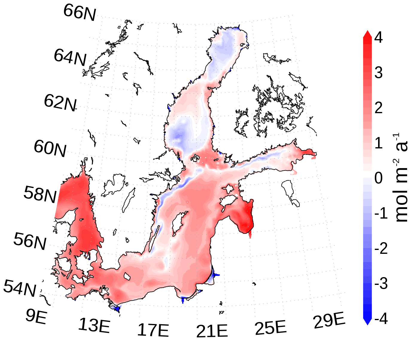
Figure 20Mean atmosphere–ocean carbon dioxide flux. A positive flux is into the Baltic Sea. The map was created using the software package GrADS 2.1.1.b0 (http://cola.gmu.edu/grads/, last access: 14 December 2021).
We compare our carbon budget with estimates from Gustafsson et al. (2017) in Table 3. The most pronounced difference is the 4-fold burial of carbon in our estimates. It corresponds to a rate of 9 . Leipe et al. (2010, Fig. 7) estimate an observation-based carbon burial rate which is similar to our rate. However, uncertainties in such rates are large, specifically due to a strong spatial heterogeneity of the carbon burial.
Table 3Total carbon budget for the whole model domain (NM) compared with estimates from Gustafsson et al. (2017, Table 6) (GS).
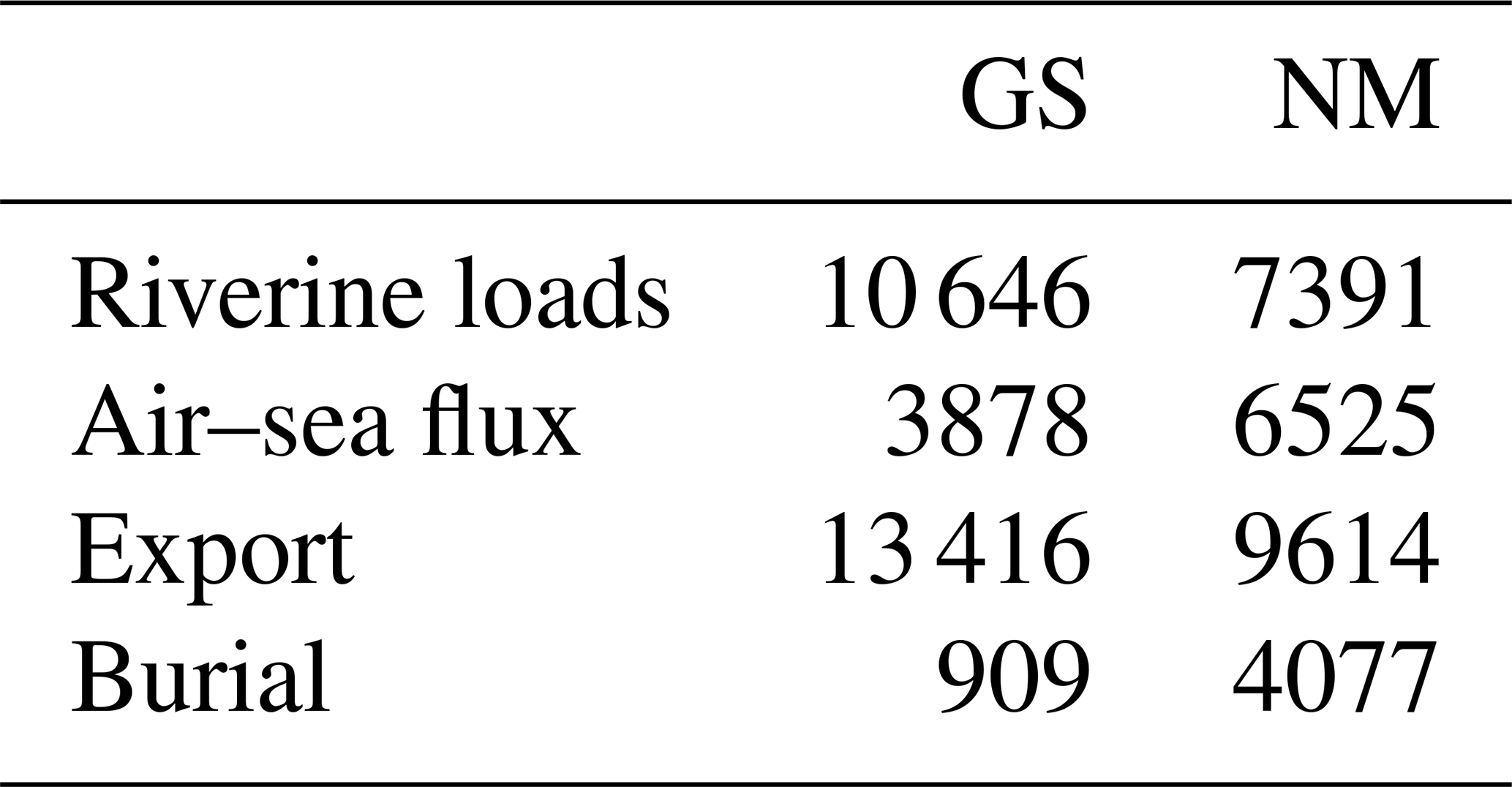
All carbon fluxes in kt a−1.
Observations of the marine carbon cycle and especially the spCO2 provide an additional, independent state variable that constrains ecosystem models. Therefore, models able to reproduce the carbon cycle in addition to e.g., nitrogen and phosphorus cycle should be more robust against changes in the forcing conditions (higher predictive capacity). This is especially important if the models will be used for projections or scenario simulations with changing forcing.
As a lot of observational effort in the past focused on nitrogen and phosphorous cycling, proper implementation of the carbon system requires additional observational and experimental data addressing the carbon cycle. For instance, the reason for the mismatch between observational and experimental alkalinity inventories needs to be addressed by re-addressing the alkalinity flux from the riverine input. Clear evidence has been provided for trends of increasing alkalinity in the major basins of the Baltic Sea (Müller et al., 2016), particularly pronounced in the northern basins, but a concerted effort to better constrain the alkalinity fluxes from the major riverine sources is currently lacking. Additional contributions from groundwater seepage can contribute to the alkalinity flux from land and have been shown to locally enhance alkalinity, but the importance on a basin-wide scale is unclear (e.g., Szymczycha et al., 2014).
The initial observational finding that carbon loss during the spring bloom continues after nitrogen depletion had originally led to the hypothesis of N fixation in late April already (Schneider et al., 2009; Kuznetsov et al., 2011), an interpretation which has been revoked by the authors due to a lack of evidence of any known N-fixing organisms during that time of the year (Schneider and Müller, 2018). However, statistical analysis of observational data clearly revealed an increase in total N in the surface waters of the central Baltic Sea during this period (Eggert and Schneider, 2015), which could not be reproduced by our model. The authors speculated about a potential vertical shuttling of nitrate by the mixotroph mesodinium rubrum, a theory later supported by observations in the Gulf of Finland (Lips and Lips, 2017). Recently, anomalously high carbon fixation in the surface layer under extreme sunny and calm spring conditions in 2018 have also been linked to potential vertical nutrient shuttling (Rehder et al., 2020). However, studies on a process level are needed to explore the mechanism and quantity of a potential nutrient shuttle.
Finally, we present a biogeochemical model for the Baltic Sea that reproduces parts of the nutrients and carbon cycle reasonably well. This progress now allows for numerical quantitative studies, especially with focus on carbon dynamics in the Baltic Sea under different forcing conditions.
In this section, we compare model results with observations in order to verify the model performance for biogeochemical variables.
A1 Surface nutrient concentrations
We demonstrate the model performance for surface nutrients at six stations and regions, respectively in Figs. A1–A6. For the climatology, we have chosen the time period 1990–2018 since observations for some stations are sparse for the period before 1990. Data for nutrients and oxygen have been extracted from the ICES database (see “Code and data availability” section).

Figure A1Surface nutrient concentrations at station BY1 (Fig. 6). The blue color represents model simulations and observations are shown as red diamonds. The blue shaded area is the range between the 10th and 90th percentiles. Opacity of the red diamonds reflects the frequency of observations. (a) Nitrate climatology. (b) Nitrate time series. (c) Phosphate climatology. (d) Phosphate time series.

Figure A2Surface nutrient concentrations at station BY5 (Fig. 6). The blue color represents model simulations and observations are shown as red diamonds. The blue shaded area is the range between the 10th and 90th percentiles. Opacity of the red diamonds reflects the frequency of observations. (a) Nitrate climatology. (b) Nitrate time series. (c) Phosphate climatology. (d) Phosphate time series.
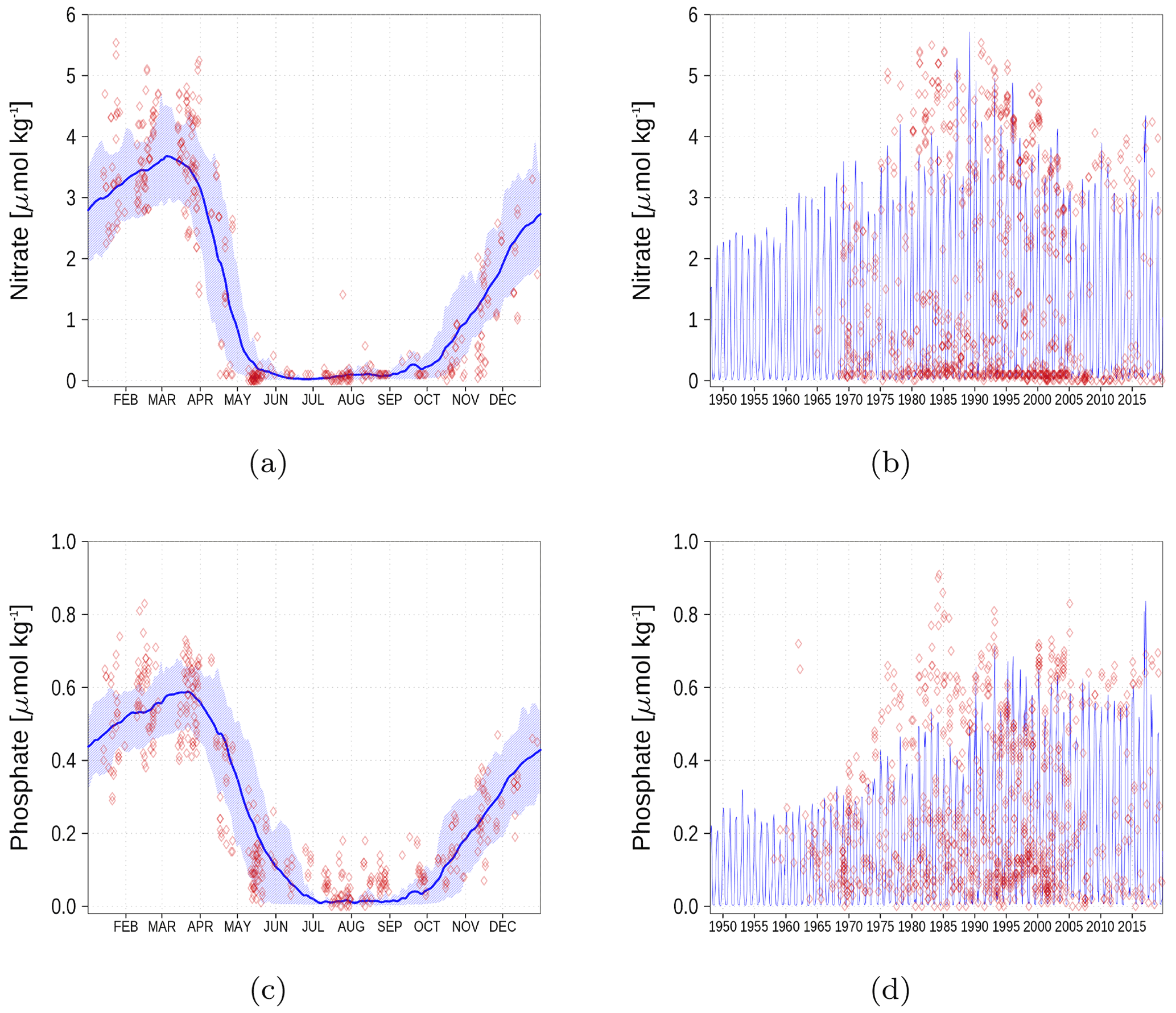
Figure A3Surface nutrient concentrations at station BY15 (Fig. 6). The blue color represents model simulations and observations are shown as red diamonds. The blue shaded area is the range between the 10th and 90th percentiles. Opacity of the red diamonds reflects the frequency of observations. (a) Nitrate climatology. (b) Nitrate time series. (c) Phosphate climatology. (d) Phosphate time series.
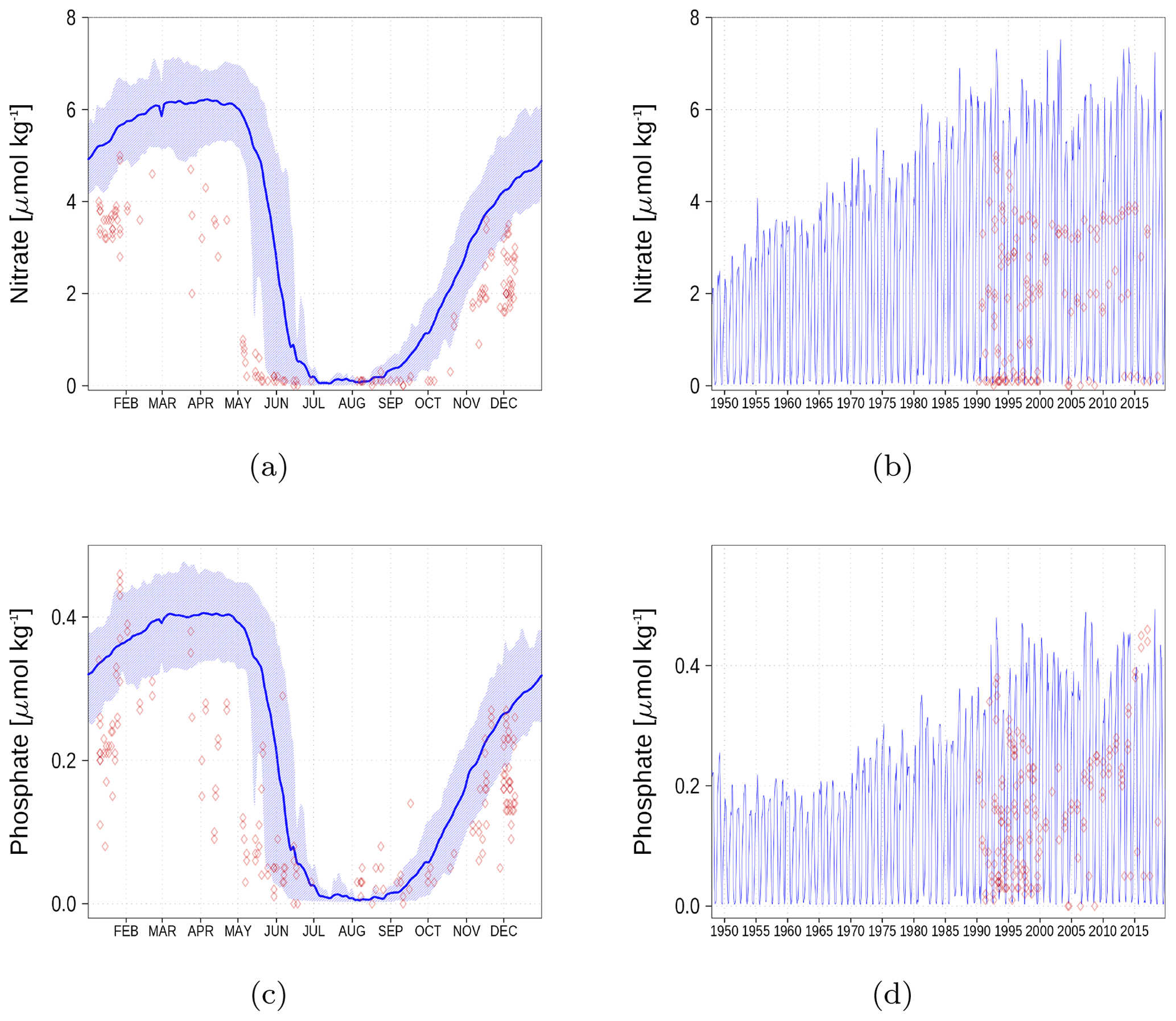
Figure A4Surface nutrient concentrations at station F26 (Fig. 6). The blue color represents model simulations and observations are shown as red diamonds. The blue shaded area is the range between the 10th and 90th percentiles. Opacity of the red diamonds reflects the frequency of observations. (a) Nitrate climatology. (b) Nitrate time series. (c) Phosphate climatology. (d) Phosphate time series.
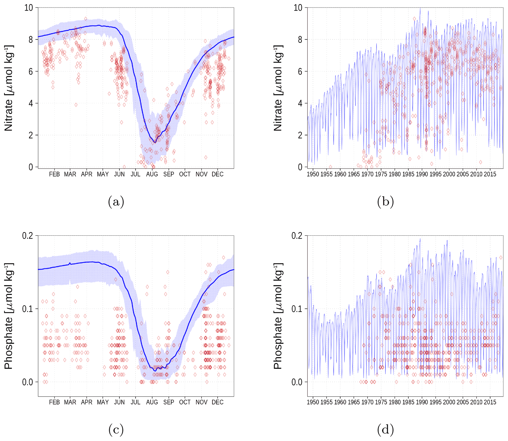
Figure A5Surface nutrient concentrations in the Bothnian Bay (BoB, Fig. 6). The blue color represents model simulations and observations are shown as red diamonds. The blue shaded area is the range between the 10th and 90th percentiles. Opacity of the red diamonds reflects the frequency of observations. (a) Nitrate climatology. (b) Nitrate time series. (c) Phosphate climatology. (d) Phosphate time series.
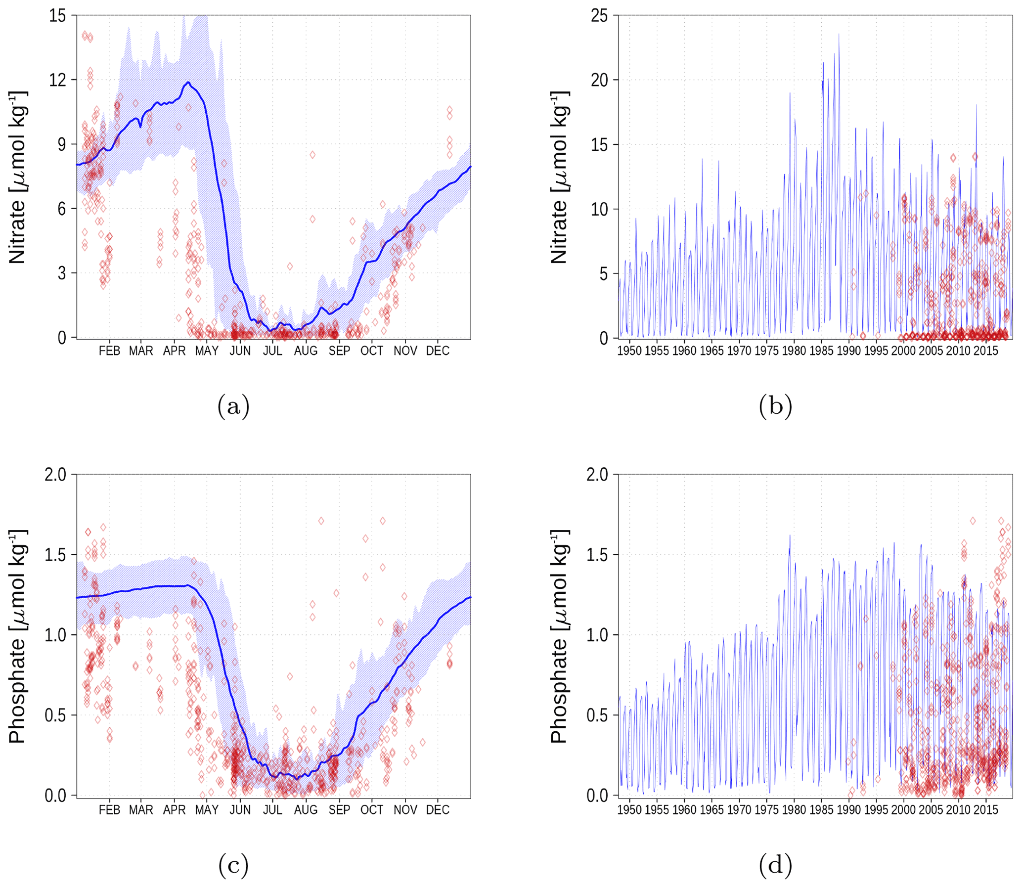
Figure A6Surface nutrient concentrations at the station in the Gulf of Finland (GoF, Fig. 6). The blue color represents model simulations and observations are shown as red diamonds. The blue shaded area is the range between the 10th and 90th percentiles. Opacity of the red diamonds reflects the frequency of observations. (a) Nitrate climatology. (b) Nitrate time series. (c) Phosphate climatology. (d) Phosphate time series.
A2 Oxygen
In Fig. A7, we show oxygen concentration close to the sea floor at six different stations together with observations. Hydrogen sulfide is represented as negative oxygen equivalents. The simulated oxygen concentration reasonably follows the observations. An exception is the underestimation in the Gulf of Bothnia (Fig. A7d and e). Beginning in 1970, the simulated values start to deviate from the field data.
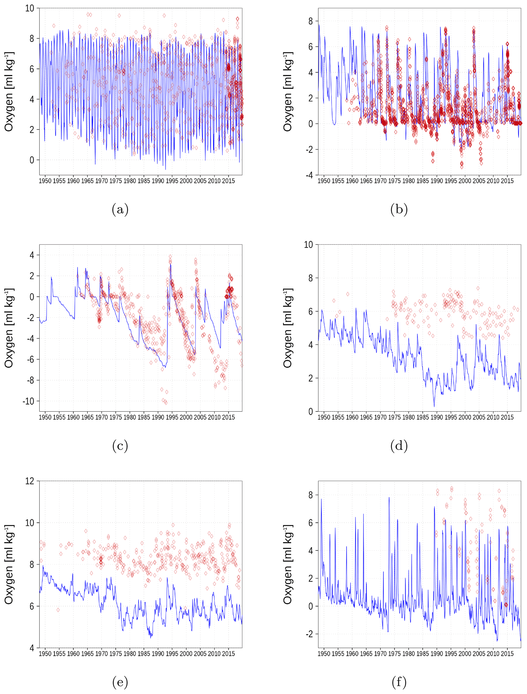
Figure A7Bottom oxygen concentration at six stations in the Baltic Sea. Negative values denote the presence of hydrogen sulfide. The blue color represents model simulations and observations are shown as red diamonds. Opacity of the red diamonds reflects the frequency of observations. (a) BY1, (b) BY5, (c) BY15, (d) F26, (e) BoB, (f) GoF (Fig. 6).
B1 Introduction
This is an automatically generated description of the ecosystem model ERGOM, version CDOM 1.2. Model formulation is provided by text files in compliance with the rules of the Code Generation Tool (CGT) by Hagen Radtke (see https://www.ergom.net, last access: 15 November 2022).
The ecosystem state variables are concentrations of several substances and are called tracers. In the host ocean model, they undergo physical advection, turbulent diffusion, or vertical motion as sinking or rising. The ecosystem model component defines their sources or sinks from elemental turnover through the ecosystem. They are defined and described in Appendix B2.
Appendix B3 is the main part of this model description document. It describes the processes changing the tracer concentrations over time. Analogously to chemical processes, two components describe a process:
-
a process equation which describes the transformation from precursors (on the left-hand side) to products (on the right-hand side), and
-
a turnover rate, describing how fast the process runs.
The time tendency of a tracer can then easily be determined by multiplying the process turnover rate with the stoichiometric ratio in which it consumes or produces the tracer according to the reaction equation.
The document structure reflects the different process types. All processes of one type (e.g., phytoplankton assimilation) are listed together with all their constants and auxiliary variables they depend on. For readability, some constants, such as stoichiometric ratios, will occur repeatedly. We take this compromise for the sake of readability, keeping all information required to understand a specific process in its own section.
For completeness, the tracer equations are given in Appendix B4. However, we consider this as a supplementary chapter and suggest studying the model details from Appendix B3 instead.
B2 Description of model state variables (tracers)
B3 Description of model processes, ordered by process type
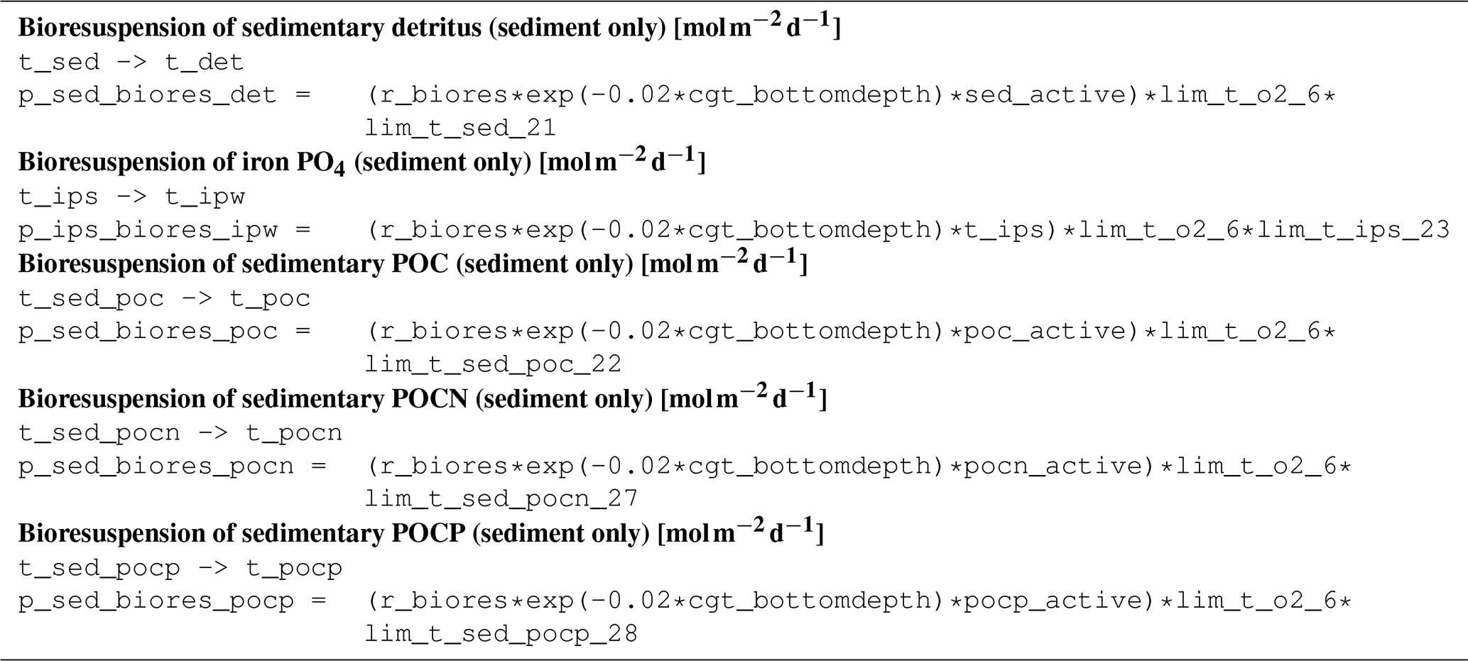
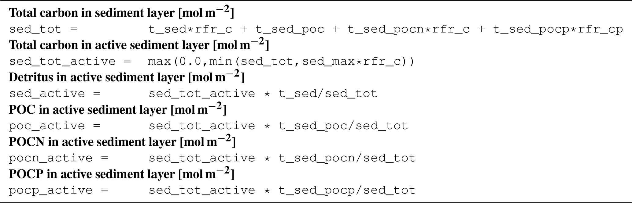
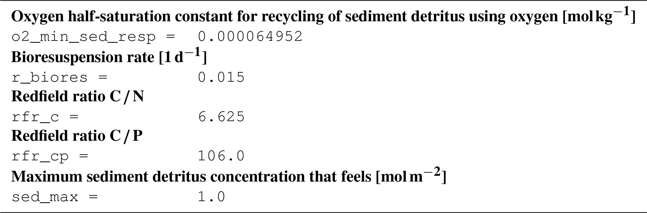
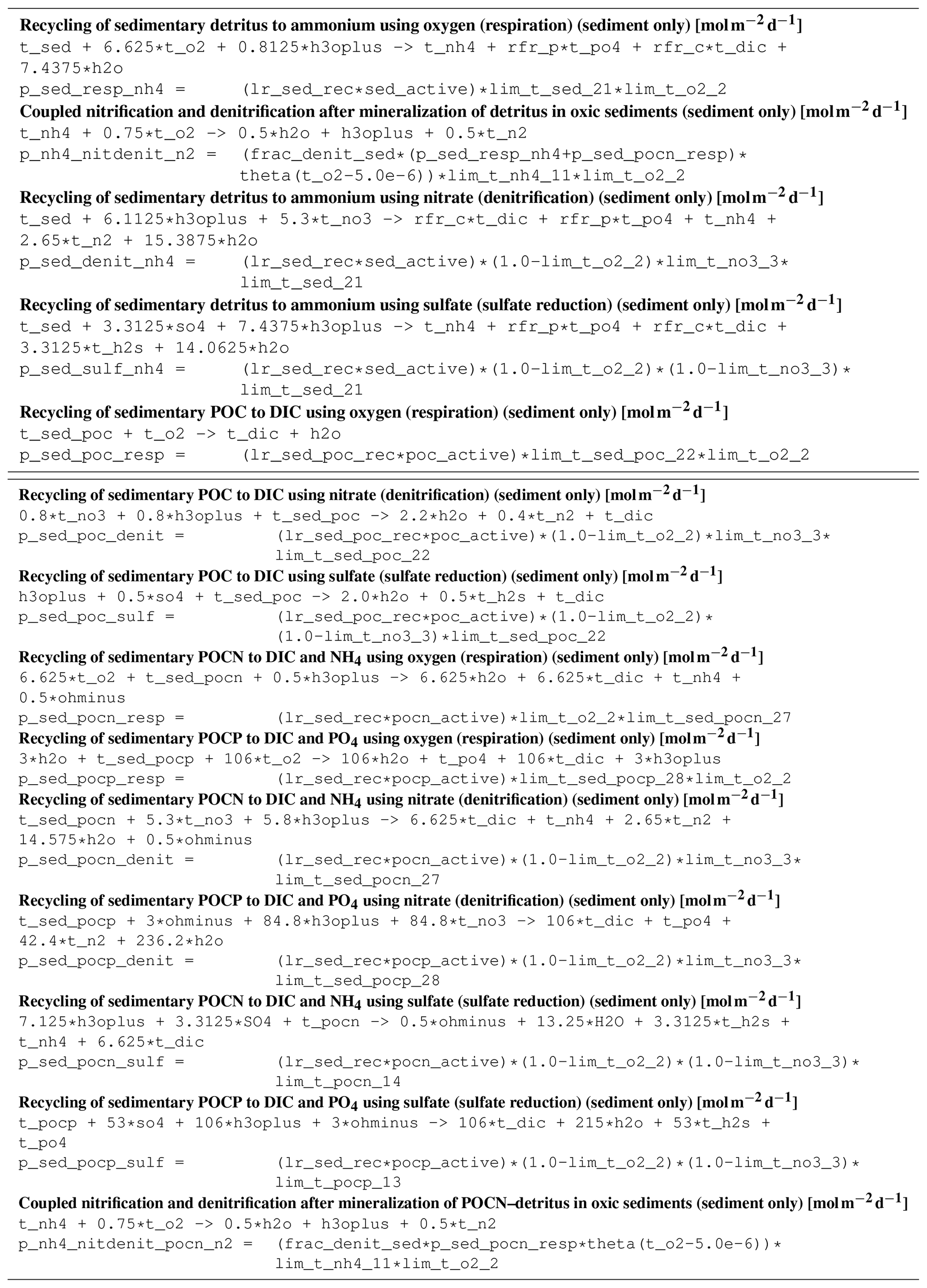
B3.1 Process type BGC/benthic/bioresuspension

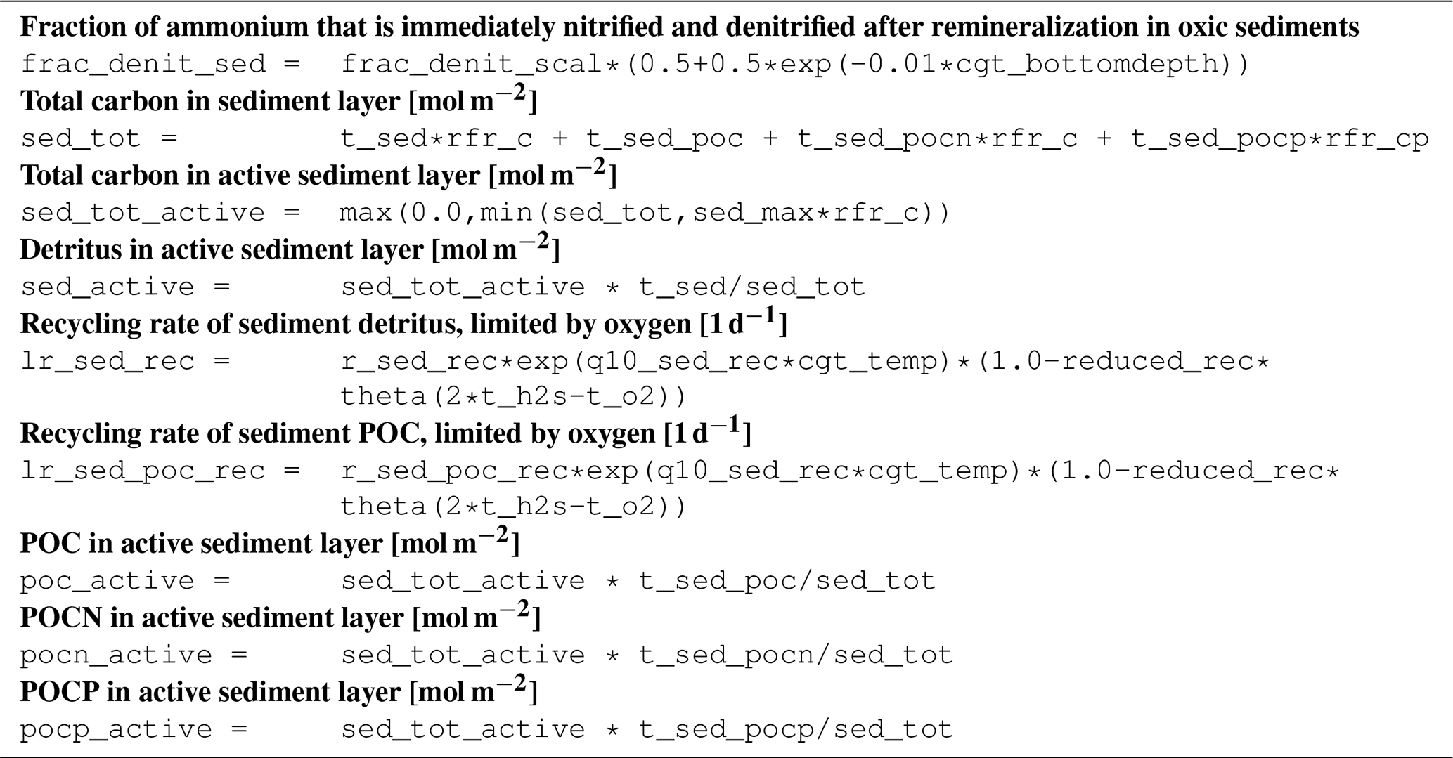
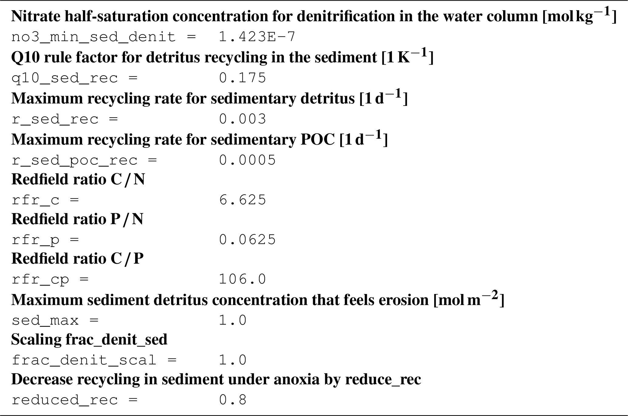
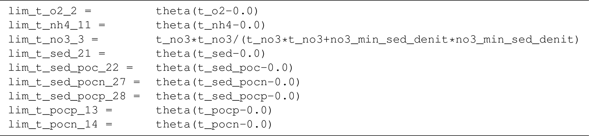
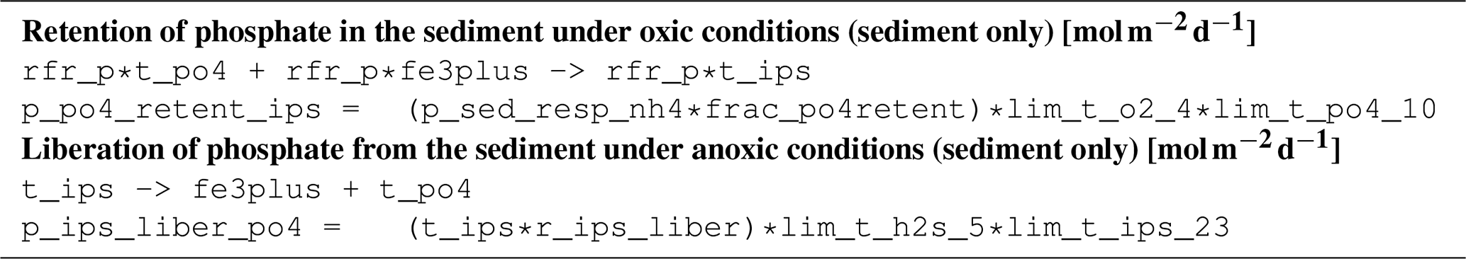
B3.2 Process type BGC/benthic/mineralisation
B3.3 Process type BGC/benthic/P_retention

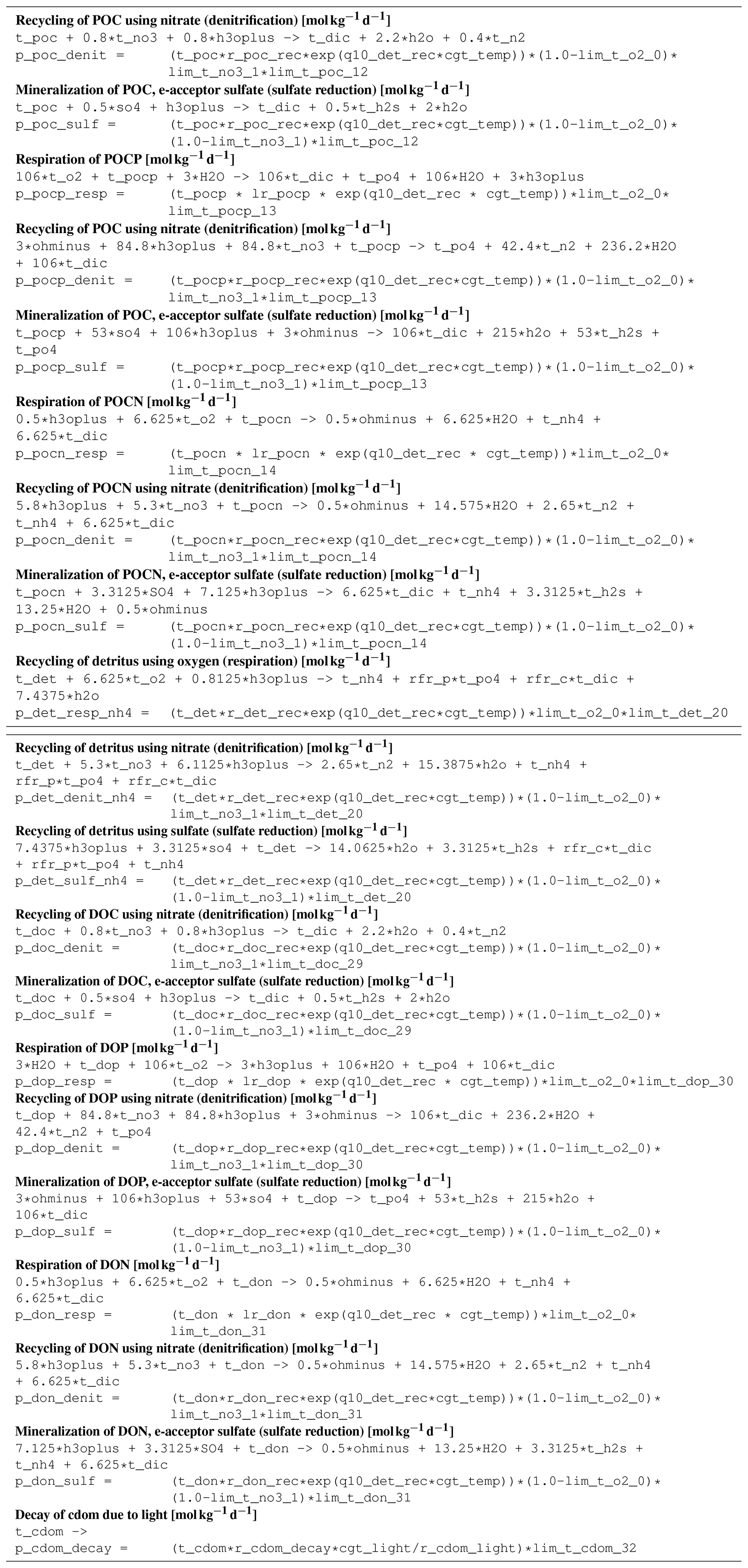
B3.4 Process type BGC/pelagic/mineralization


B3.5 Process type BGC/pelagic/phytoplankton
B3.6 Process type BGC/pelagic/reoxidation

B3.7 Process type BGC/pelagic/zooplankton
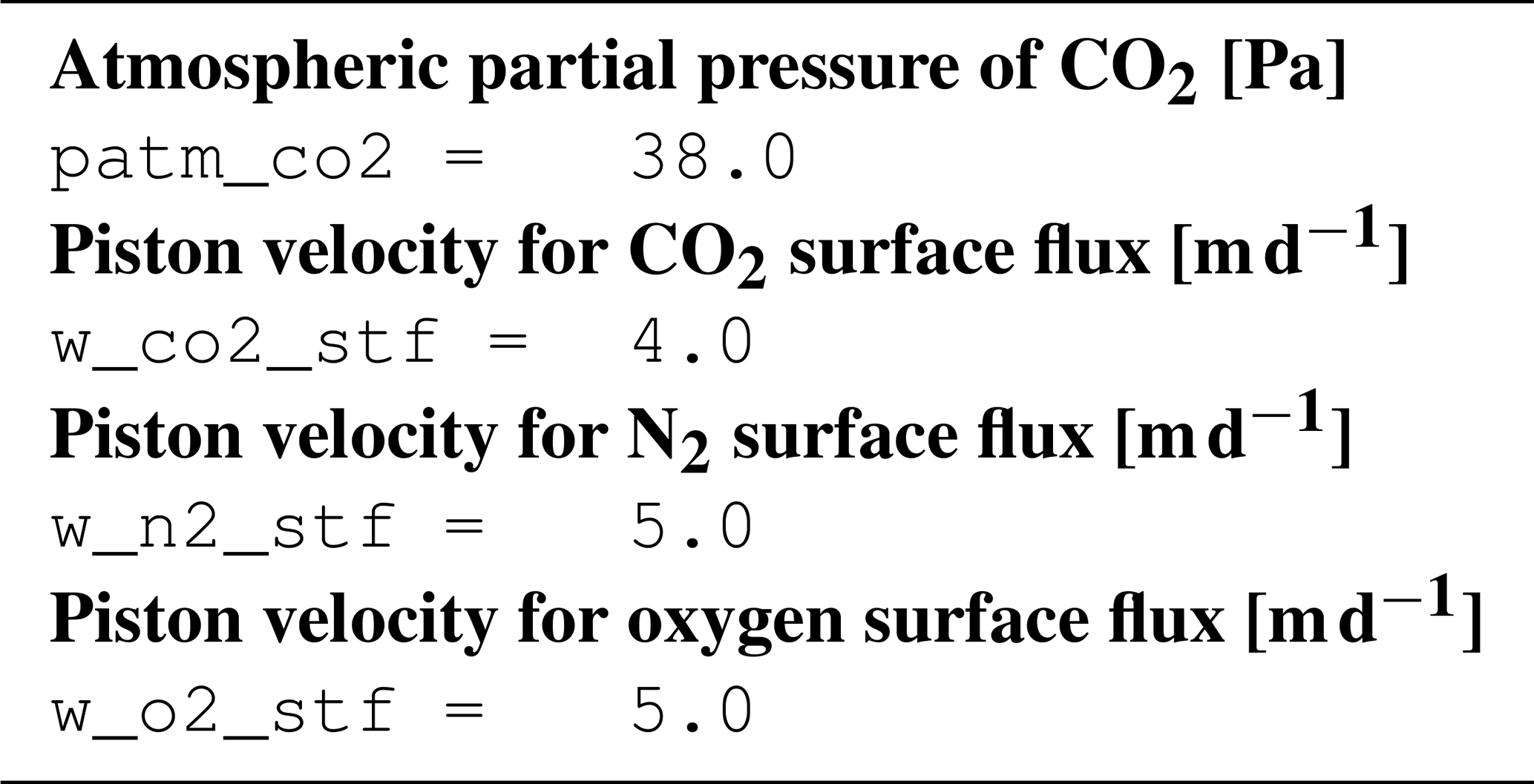
B3.8 Process type gas_exchange

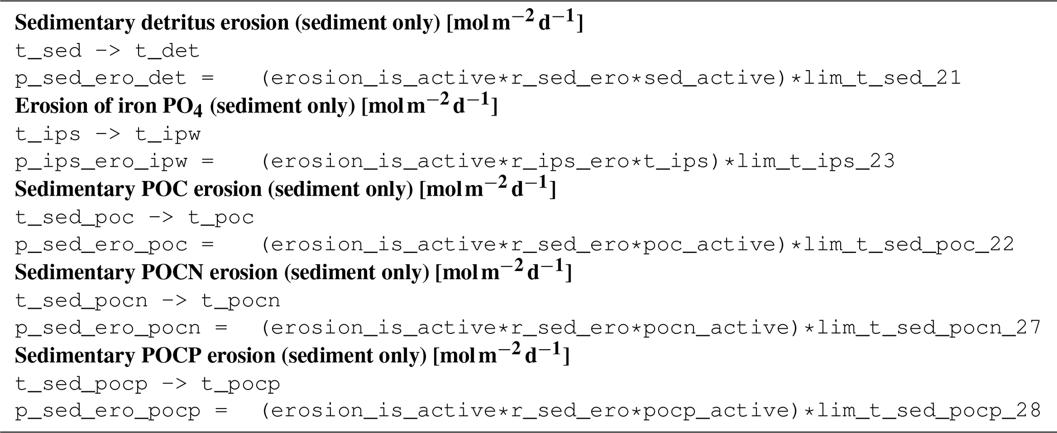
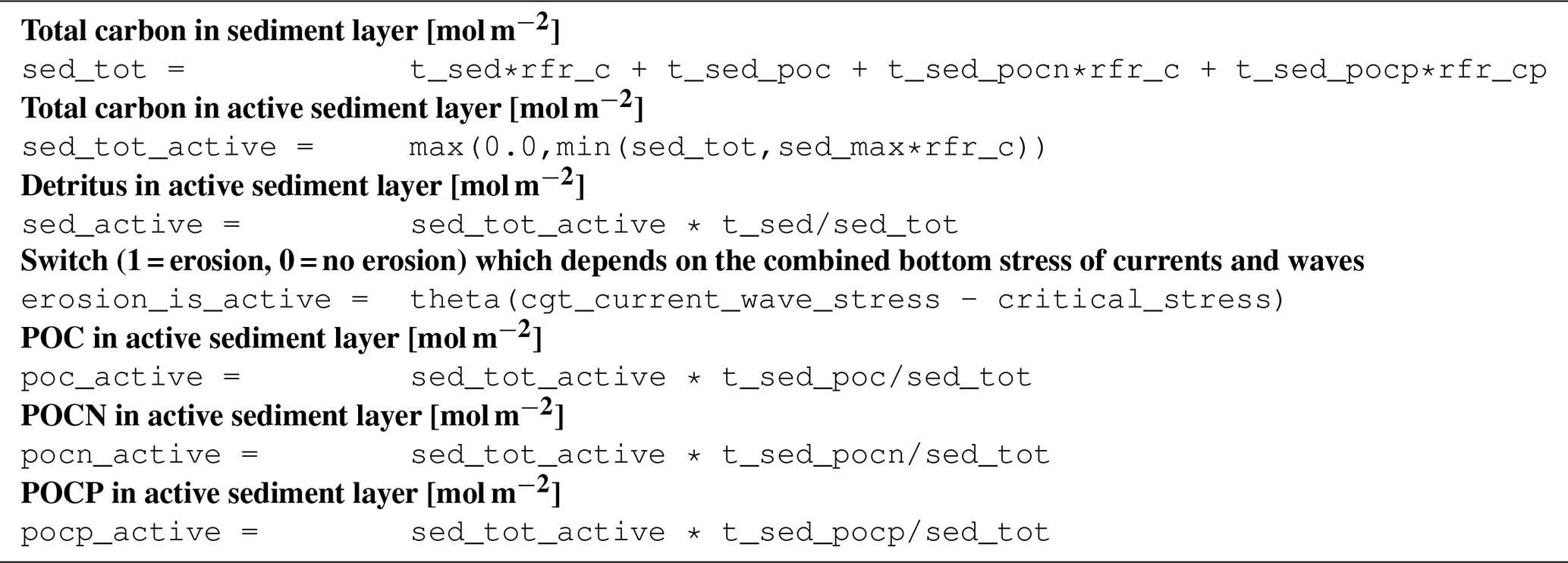
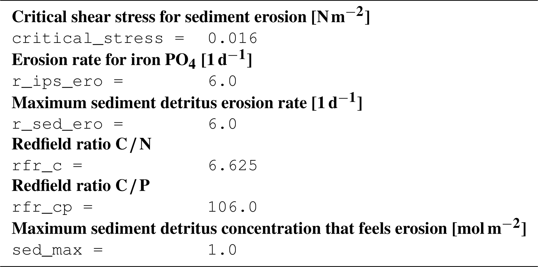
B3.9 Process type physics/erosion
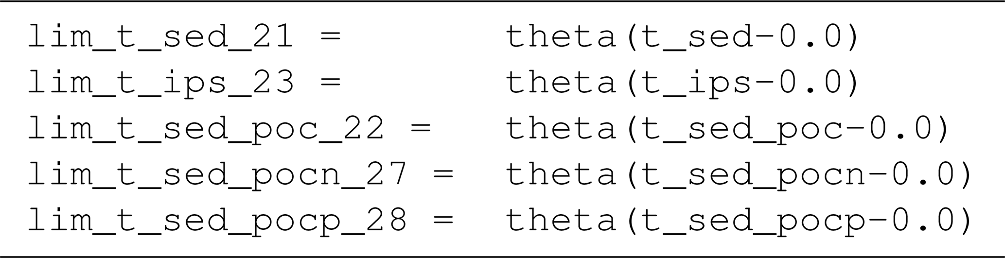
B3.10 Process type physics/parameterization_deep_burial
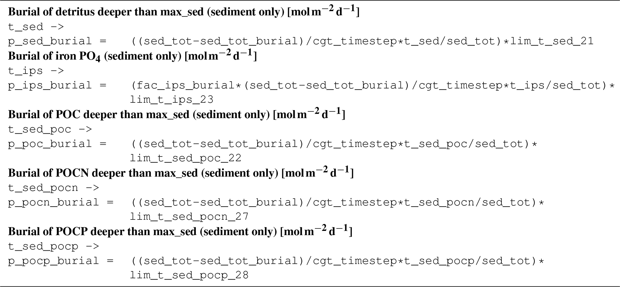

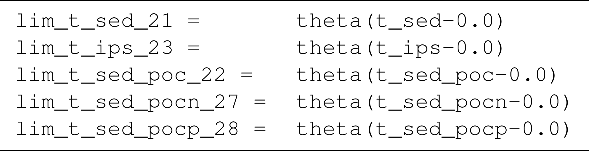
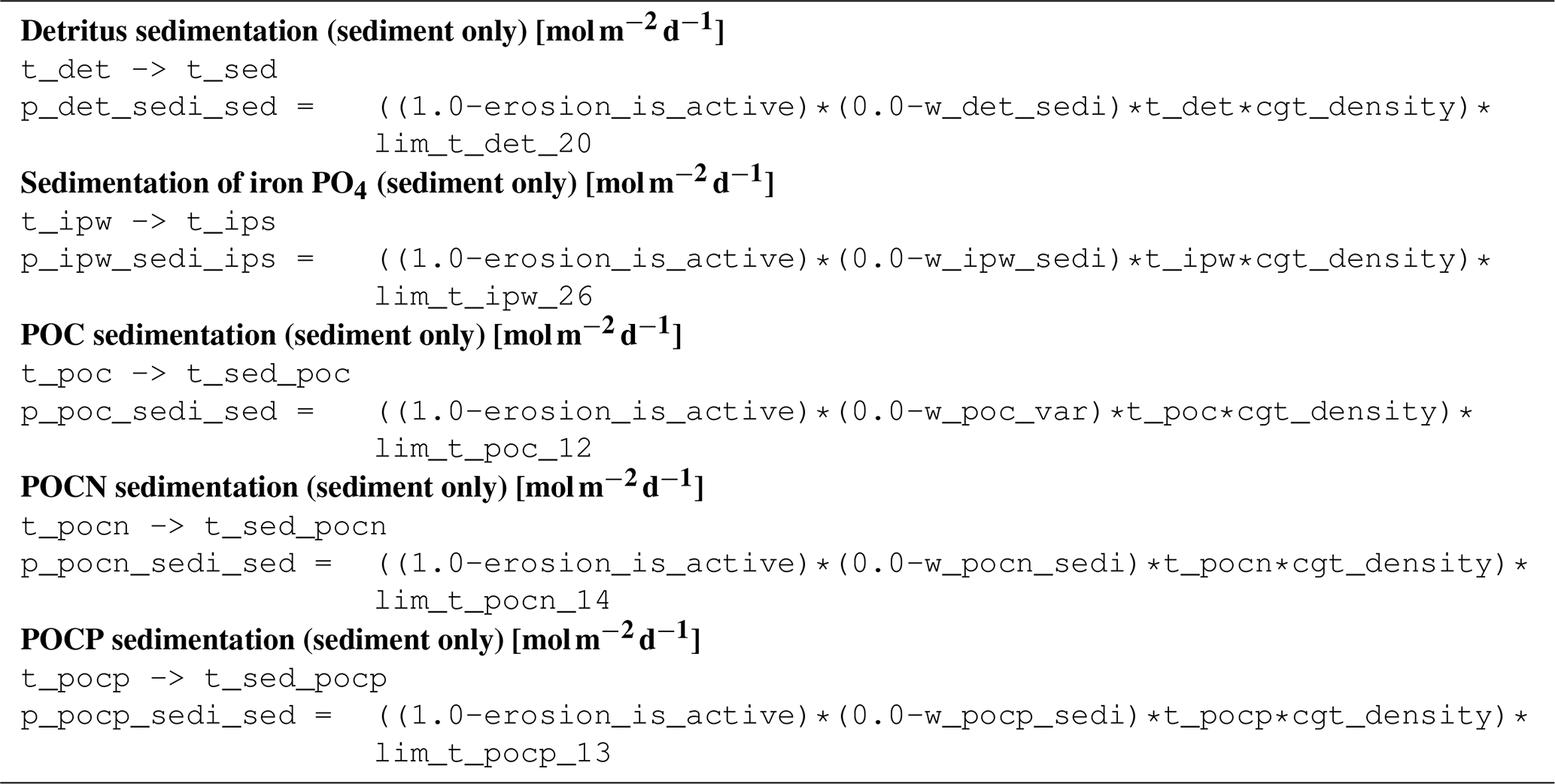
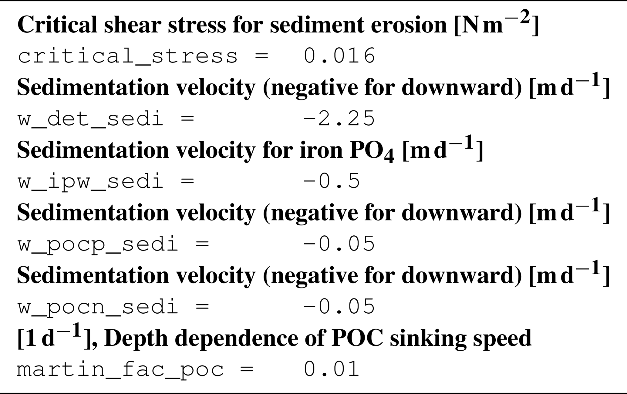
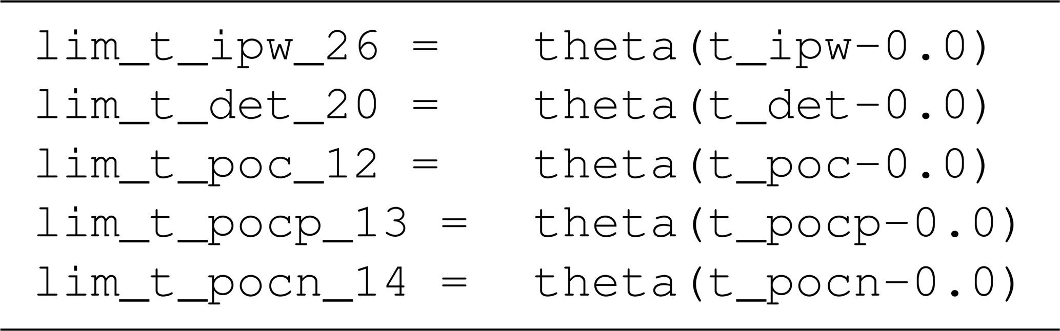
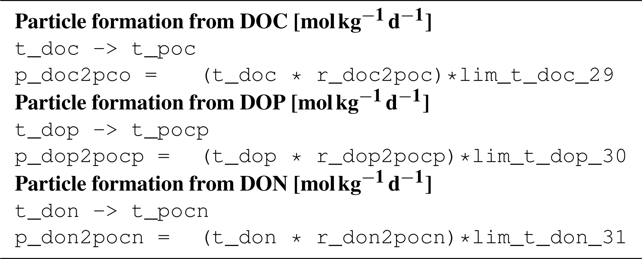
B3.11 Process type physics/sedimentation

B3.12 Process type standard
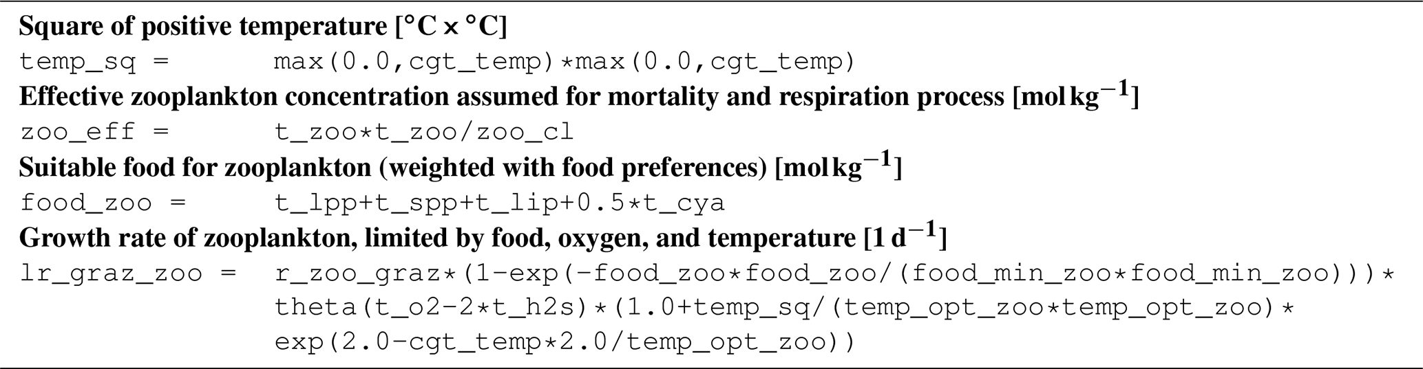
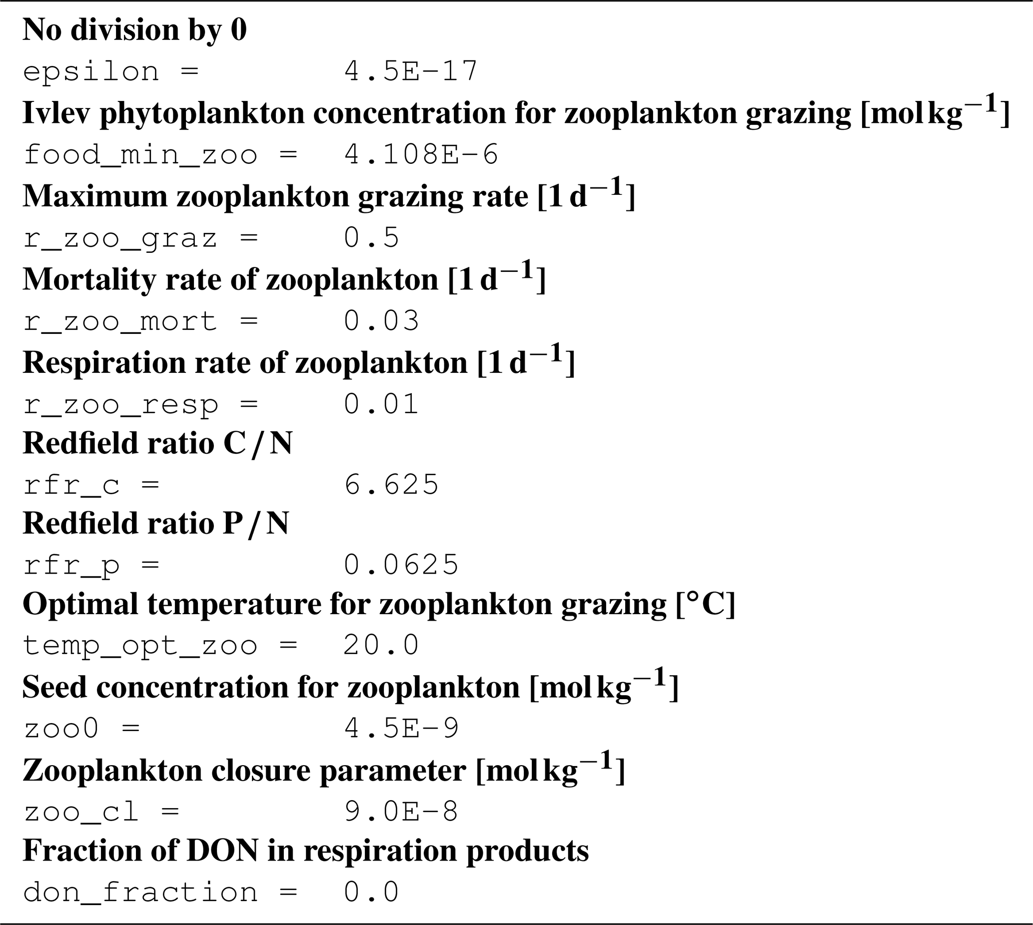
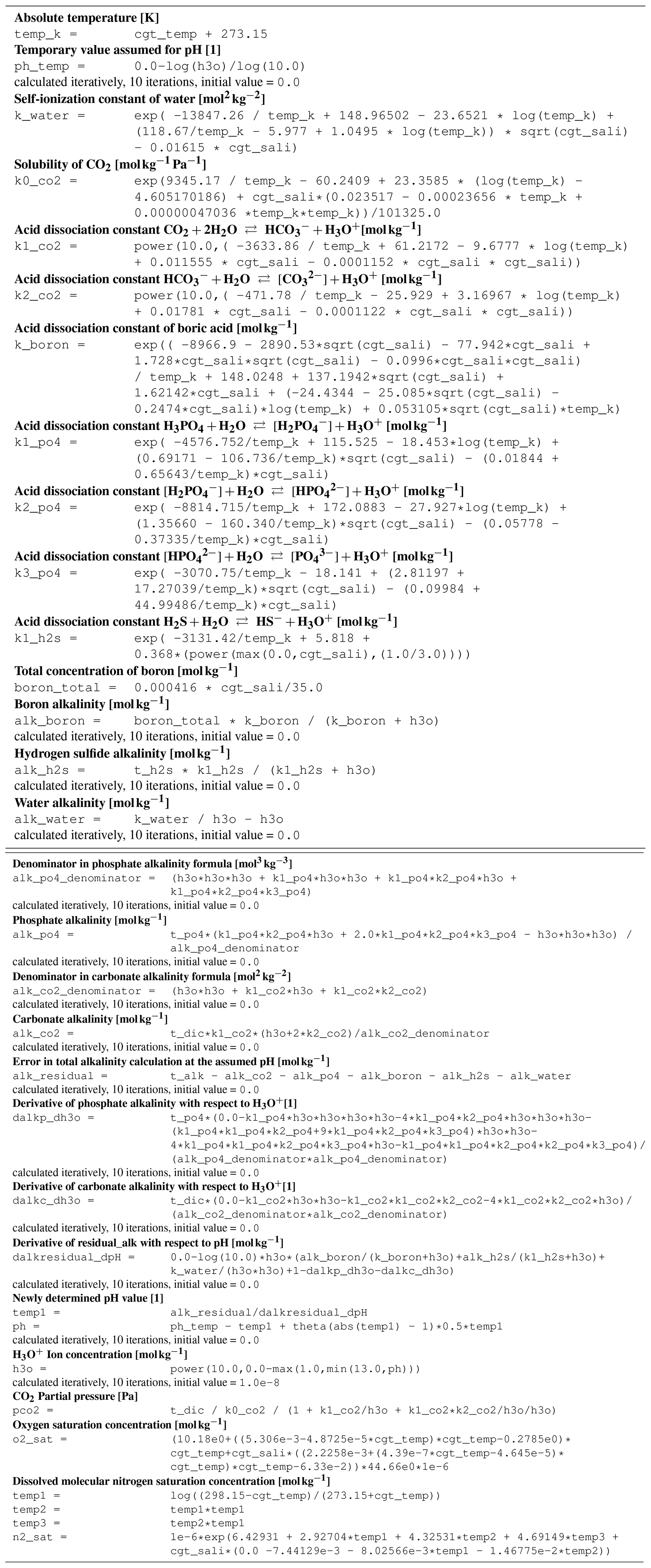
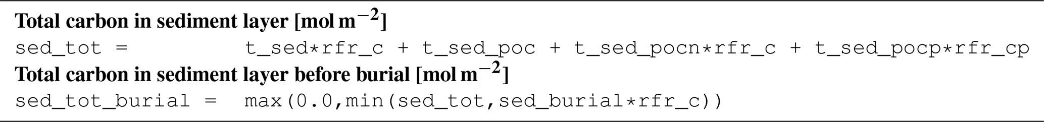
B4 Tracer equations

spCO2 data used are available from https://doi.org/10.25921/1h9f-nb73 (Bakker et al., 2022). Oceanographic nutrient and oxygen data used for model validation are available from https://www.ices.dk/data/data-portals/Pages/default.aspx (ICES, 2022). DOC data used are available from the IOW database ODIN https://odin2.io-warnemuende.de/ (Leibniz Institute for Baltic Sea Research, 2022). Alkalinity data used are available from the SHARK database https://sharkweb.smhi.se/hamta-data/ (The Swedish Agency for Marine and Water Management and the Swedish Meteorological and Hydrological Institute, 2022). The meteorological forcing is archived at https://doi.org/10.1594/WDCC/coastDat-2_COSMO-CLM (last access: 14 January 2022, Geyer and Rockel, 2013).
The code of the biogeochemical model is available at https://ergom.net/ (Leibniz Institute for Baltic Sea Research, 2015). The ocean model “Modular Ocean Model MOM 5-1”, used in this study, is available from the developers repository https://github.com/mom-ocean/MOM5 (last access: 14 January 2022).
Model data can be accessed via https://thredds-iow.io-warnemuende.de/thredds/catalogs/projects/integral/catalog_pocNP_V04R25_3nm_agg_time.html (last access: 14 January 2022, Neumann, 2021). All data used in this study for analysis and figures are archived on Zenodo at https://doi.org/10.5281/zenodo.7252134 (last access: 26 October 2022, Neumann, 2022).
The version of the model code used to produce the results in this study is archived on Zenodo at https://doi.org/10.5281/zenodo.7252134 (last access: 26 October 2022, Neumann, 2022). In addition to the source code, the archive includes initial fields and boundary conditions, except the meteorological forcing.
TN, HR, BC, and MS developed and implemented the model. TN performed the model simulations. All the authors contributed to writing the manuscript.
The contact author has declared that none of the authors has any competing interests.
Publisher's note: Copernicus Publications remains neutral with regard to jurisdictional claims in published maps and institutional affiliations.
Computational power was provided by the North-German Supercomputing Alliance (HLRN).This study was part of the BONUS INTEGRAL 363 project. We wish to thank Bernd Schneider and Henry Bitting for many pieces of advice and discussion.
This research has been supported by the Bundesministerium für Bildung und Forschung (grant no. 03F0773A).
The publication of this article was funded by the Open Access Fund of the Leibniz Association.
This paper was edited by Andrew Yool and reviewed by Tatsuro Tanioka and Feifei Liu.
Bakker, D. C. E., Pfeil, B., Landa, C. S., Metzl, N., O'Brien, K. M., Olsen, A., Smith, K., Cosca, C., Harasawa, S., Jones, S. D., Nakaoka, S., Nojiri, Y., Schuster, U., Steinhoff, T., Sweeney, C., Takahashi, T., Tilbrook, B., Wada, C., Wanninkhof, R., Alin, S. R., Balestrini, C. F., Barbero, L., Bates, N. R., Bianchi, A. A., Bonou, F., Boutin, J., Bozec, Y., Burger, E. F., Cai, W.-J., Castle, R. D., Chen, L., Chierici, M., Currie, K., Evans, W., Featherstone, C., Feely, R. A., Fransson, A., Goyet, C., Greenwood, N., Gregor, L., Hankin, S., Hardman-Mountford, N. J., Harlay, J., Hauck, J., Hoppema, M., Humphreys, M. P., Hunt, C. W., Huss, B., Ibánhez, J. S. P., Johannessen, T., Keeling, R., Kitidis, V., Körtzinger, A., Kozyr, A., Krasakopoulou, E., Kuwata, A., Landschützer, P., Lauvset, S. K., Lefèvre, N., Lo Monaco, C., Manke, A., Mathis, J. T., Merlivat, L., Millero, F. J., Monteiro, P. M. S., Munro, D. R., Murata, A., Newberger, T., Omar, A. M., Ono, T., Paterson, K., Pearce, D., Pierrot, D., Robbins, L. L., Saito, S., Salisbury, J., Schlitzer, R., Schneider, B., Schweitzer, R., Sieger, R., Skjelvan, I., Sullivan, K. F., Sutherland, S. C., Sutton, A. J., Tadokoro, K., Telszewski, M., Tuma, M., van Heuven, S. M. A. C., Vandemark, D., Ward, B., Watson, A. J., and Xu, S.: A multi-decade record of high-quality fCO2 data in version 3 of the Surface Ocean CO2 Atlas (SOCAT), Earth Syst. Sci. Data, 8, 383–413, https://doi.org/10.5194/essd-8-383-2016, 2016. a
Bakker, D. C. E., Alin, S. R., Becker, M., Bittig, H. C., Castaño-Primo, R., Feely, R. A., Gkritzalis, T., Kadono, K., Kozyr, A., Lauvset, S. K., Metzl, N., Munro, D. R., Nakaoka, S., Nojiri, Y., O'Brien, K. M., Olsen, A., Pfeil, B., Pierrot, D., Steinhoff, T., Sullivan, K. F., Sutton, A. J., Sweeney, C., Tilbrook, B., Wada, C., Wanninkhof, R., Willstrand W., Anna, A., John, A., L. B., Bates, N., Beatty, C. M., Burger, E. F., Cai, W.-J., Cosca, C. E., Corredor, J. E., Cronin, M., Cross, J. N., De Carlo, E. H., DeGrandpre, M. D., Emerson, S., Enright, M. P., Enyo, K., Evans, W., Frangoulis, C., Fransson, A., García-Ibáñez, M. I., Gehrung, M., Giannoudi, L., Glockzin, M., Hales, B., Howden, S. D., Hunt, C. W., Ibánhez, J. S. P., Jones, S. D., Kamb, L., Körtzinger, A., Landa, C. S., Landschützer, P., Lefèvre, N., Lo Monaco, C., Macovei, V. A., Maenner Jones, S., Meinig, C., Millero, F. J., Monacci, N. M., Mordy, C., Morell, J. M., Murata, A., Musielewicz, S., Neill, C., Newberger, T., Nomura, D., Ohman, M., Ono, T., Passmore, A., Petersen, W., Petihakis, G., Perivoliotis, L., Plueddemann, A. J., Rehder, G., Reynaud, T., Rodriguez, C., Ross, A. C., Rutgersson, A., Sabine, C. L., Salisbury, J. E., Schlitzer, R., Send, U., Skjelvan, I., Stamataki, N., Sutherland, S. C., Sweeney, C., Tadokoro, K., Tanhua, T., Telszewski, M., Trull, T., Vandemark, D., van Ooijen, E., Voynova, Y. G., Wang, H., Weller, R. A., Whitehead, C., and Wilson, D.: Surface Ocean CO2 Atlas Database Version 2022 (SOCATv2022) (NCEI Accession 0253659), NOAA National Centers for Environmental Information [data set], https://doi.org/10.25921/1h9f-nb73, 2022. a
Carlson, C. A. and Hansell, D. A.: Chapter 3 – DOM Sources, Sinks, Reactivity, and Budgets, in: Biogeochemistry of Marine Dissolved Organic Matter, 2nd edn., edited by: Carlson, D. A. and Hansell, C. A., Academic Press, Boston, 65–126, https://doi.org/10.1016/B978-0-12-405940-5.00003-0, 2015. a, b
Carlson, C. A., Ducklow, H. W., Hansell, D. A., and Smith Jr., W. O.: Organic carbon partitioning during spring phytoplankton blooms in the Ross Sea polynya and the Sargasso Sea, Limnol. Oceanogr., 43, 375–386, https://doi.org/10.4319/lo.1998.43.3.0375, 1998. a
Chien, C.-T., Pahlow, M., Schartau, M., and Oschlies, A.: Optimality-based non-Redfield plankton–ecosystem model (OPEM v1.1) in UVic-ESCM 2.9 – Part 2: Sensitivity analysis and model calibration, Geosci. Model Dev., 13, 4691–4712, https://doi.org/10.5194/gmd-13-4691-2020, 2020. a
Droop, M. R.: Some Thoughts on Nutrient Limitation in Algae, J. Phycol., 9, 264–272, https://doi.org/10.1111/j.1529-8817.1973.tb04092.x, 1973. a
Eggert, A. and Schneider, B.: A nitrogen source in spring in the surface mixed-layer of the Baltic Sea: Evidence from total nitrogen and total phosphorus data, J. Marine Syst., 148, 39–47, https://doi.org/10.1016/j.jmarsys.2015.01.005, 2015. a
Engel, A.: Direct relationship between CO2 uptake and transparent exopolymer particles production in natural phytoplankton, J. Plankton Res., 24, 49–53, https://doi.org/10.1093/plankt/24.1.49, 2002. a, b
Engel, A., Thoms, S., Riebesell, U., Rochelle-Newall, E., and Zondervan, I.: Polysaccharide aggregation as a potential sink of marine dissolved organic carbon, Nature, 428, 929–932, https://doi.org/10.1038/nature02453, 2004. a
Eppley, R. W.: Temperature and phytoplankton growth, Fish. Bull., 70, 1063–1085, 1972. a
Fransner, F., Gustafsson, E., Tedesco, L., Vichi, M., Hordoir, R., Roquet, F., Spilling, K., Kuznetsov, I., Eilola, K., Mörth, C.-M., Humborg, C., and Nycander, J.: Non-Redfieldian Dynamics Explain Seasonal pCO2 Drawdown in the Gulf of Bothnia, J. Geophys. Res.-Oceans, 123, 166–188, https://doi.org/10.1002/2017JC013019, 2018. a, b, c, d, e, f, g
Geyer, B. and Rockel, B.: coastDat-2 COSMO-CLM Atmospheric Reconstruction [data set], https://doi.org/10.1594/WDCC/coastDat-2_COSMO-CLM, 2013. a, b
Griffies, S. M.: Fundamentals of Ocean Climate Models, Princeton University Press, Princeton, NJ, ISBN 9780691118925, 2004. a
Gustafsson, E., Deutsch, B., Gustafsson, B., Humborg, C., and Mörth, C.-M.: Carbon cycling in the Baltic Sea? The fate of allochthonous organic carbon and its impact on air-sea CO2 exchange, J. Marine Syst., 129, 289–302, https://doi.org/10.1016/j.jmarsys.2013.07.005, 2014a. a
Gustafsson, E., Wällstedt, T., Humborg, C., Mörth, C.-M., and Gustafsson, B. G.: External total alkalinity loads versus internal generation: The influence of nonriverine alkalinity sources in the Baltic Sea, Global Biogeochem. Cy., 28, 1358–1370, https://doi.org/10.1002/2014GB004888, 2014b. a, b, c, d, e, f
Gustafsson, E., Savchuk, O. P., Gustafsson, B. G., and Müller-Karulis, B.: Key processes in the coupled carbon, nitrogen, and phosphorus cycling of the Baltic Sea, Biogeochemistry, 134, 301–317, https://doi.org/10.1007/s10533-017-0361-6, 2017. a, b
Gustafsson, E., Hagens, M., Sun, X., Reed, D. C., Humborg, C., Slomp, C. P., and Gustafsson, B. G.: Sedimentary alkalinity generation and long-term alkalinity development in the Baltic Sea, Biogeosciences, 16, 437–456, https://doi.org/10.5194/bg-16-437-2019, 2019. a, b
Hansell, D. A., Carlson, C. A., Repeta, D. J., and Schlitzer, R.: Dissolved Organic Matter in the Ocean: A Controversy Stimulates New Insights, Oceanography, 22, 202–211, https://doi.org/10.5670/oceanog.2009.109, 2009. a
HELCOM: Sources and pathways of nutrients to the Baltic Sea, Balt. Sea Environ. Proc. No. 153, HELCOM, ISSN 0357-2994, https://helcom.fi/wp-content/uploads/2019/08/BSEP153.pdf (last access: 15 November 2022), 2018. a
Hjalmarsson, S., Wesslander, K., Anderson, L. G., Omstedt, A., Perttilä, M., and Mintrop, L.: Distribution, long-term development and mass balance calculation of total alkalinity in the Baltic Sea, Cont. Shelf Res., 28, 593–601, https://doi.org/10.1016/j.csr.2007.11.010, 2008. a, b, c, d, e
Ho, T.-Y., Quigg, A., Finkel, Z. V., Milligan, A. J., Wyman, K., Falkowski, P. G., and Morel, F. M. M.: The Elemental Composition of Some Marine Phytoplankton, J. Phycol., 39, 1145–1159, https://doi.org/10.1111/j.0022-3646.2003.03-090.x, 2003. a
Hoikkala, L., Kortelainen, P., Soinne, H., and Kuosa, H.: Dissolved organic matter in the Baltic Sea, J. Marine Syst., 142, 47–61, https://doi.org/10.1016/j.jmarsys.2014.10.005, 2015. a
ICES: Database Oceanography [data set], https://www.ices.dk/data/data-portals/Pages/default.aspx, last access: 14 January 2022. a
Kreus, M., Schartau, M., Engel, A., Nausch, M., and Voss, M.: Variations in the elemental ratio of organic matter in the central Baltic Sea: Part I – Linking primary production to remineralization, Cont. Shelf Res., 100, 25–45, https://doi.org/10.1016/j.csr.2014.06.015, 2015. a, b, c
Kriest, I., Oschlies, A., and Khatiwala, S.: Sensitivity analysis of simple global marine biogeochemical models, Global Biogeochem. Cy., 26, GB2029, https://doi.org/10.1029/2011GB004072, 2012. a
Kuznetsov, I., Neumann, T., and Burchard, H.: Model study on the ecosystem impact of a variable ratio for cyanobacteria in the Baltic Proper, Ecol. Model., 219, 107–114, https://doi.org/10.1016/j.ecolmodel.2008.08.002, 2008. a, b
Kuznetsov, I., Neumann, T., Schneider, B., and Yakushev, E.: Processes regulating pCO2 in the surface waters of the central eastern Gotland Sea: a model study, Oceanologia, 53, 745–770, https://doi.org/10.5697/oc.53-3.745, 2011. a, b, c, d, e, f, g
Larsson, U., Hajdu, S., Walve, J., and Elmgren, R.: Baltic Sea nitrogen fixation estimated from the summer increase in upper mixed layer total nitrogen, Limnol. Oceanogr., 46, 811–820, https://doi.org/10.4319/lo.2001.46.4.0811, 2001. a, b, c
Leibniz Institute for Baltic Sea Research: ERGOM: Ecological ReGional Ocean Model [code], https://ergom.net/ (last access: 10 March 2022), 2015. a, b, c
Leibniz Institute for Baltic Sea Research: Oceanographic Database Search with Interactive Navigation (ODIN) [data set], https://odin2.io-warnemuende.de/, last access: 15 November 2022. a
Leipe, T., Tauber, F., Vallius, H., Virtasalo, J., Uścinowicz, S., Kowalski, N., Hille, S., Lindgren, S., and Myllyvirta, T.: Particulate organic carbon (POC) in surface sediments of the Baltic Sea, Geo-Mar. Lett., 31, 175–188, https://doi.org/10.1007/s00367-010-0223-x, 2010. a
Lips, I. and Lips, U.: The Importance of Mesodinium rubrum at Post-Spring Bloom Nutrient and Phytoplankton Dynamics in the Vertically Stratified Baltic Sea, Frontiers in Marine Science, 4, 407, https://doi.org/10.3389/fmars.2017.00407, 2017. a
Macias, D., Huertas, I. E., Garcia-Gorriz, E., and Stips, A.: Non-Redfieldian dynamics driven by phytoplankton phosphate frugality explain nutrient and chlorophyll patterns in model simulations for the Mediterranean Sea, Prog. Oceanogr., 173, 37–50, https://doi.org/10.1016/j.pocean.2019.02.005, 2019. a
Martin, J. H., Knauer, G. A., Karl, D. M., and Broenkow, W. W.: VERTEX: carbon cycling in the northeast Pacific, Deep-Sea Res., 34, 267–285, https://doi.org/10.1016/0198-0149(87)90086-0, 1987. a
Martiny, A. C., Talarmin, A., Mouginot, C., Lee, J. A., Huang, J. S., Gellene, A. G., and Caron, D. A.: Biogeochemical interactions control a temporal succession in the elemental composition of marine communities, Limnol. Oceanogr., 61, 531–542, https://doi.org/10.1002/lno.10233, 2016. a
Monod, J.: The growth of bacterial cultures, Ann. Rev. Microbiol., 3, 371–394, 1949. a
Müller, J. D., Schneider, B., and Rehder, G.: Long-term alkalinity trends in the Baltic Sea and their implications for CO2-induced acidification, Limnol. Oceanogr., 61, 1984–2002, https://doi.org/10.1002/lno.10349, 2016. a
Nausch, M., Nausch, G., Lass, H. U., Mohrholz, V., Nagel, K., Siegel, H., and Wasmund, N.: Phosphorus input by upwelling in the eastern Gotland Basin (Baltic Sea) in summer and its effects on filamentous cyanobacteria, Estuar. Coast. Shelf S., 83, 434–442, https://doi.org/10.1016/j.ecss.2009.04.031, 2009. a
Neumann, T.: ERGOM 1.2 model hindcast 1948–2019 [data set], https://thredds-iow.io-warnemuende.de/thredds/catalogs/projects/integral/catalog_pocNP_V04R25_3nm_agg_time.html (last access: 10 March 2022), 2021. a
Neumann, T.: Model code and boundary data for “Non-Redfield carbon model for the Baltic Sea (ERGOM version 1.2) – Implementation and Budget estimates” paper [code], https://doi.org/10.5281/zenodo.7252134, last access: 26 October 2022. a, b
Neumann, T., Fennel, W., and Kremp, C.: Experimental simulations with an ecosystem model of the Baltic Sea: A nutrient load reduction experiment, Global Biogeochem. Cy., 16, 7-1–7-19, https://doi.org/10.1029/2001GB001450, 2002. a
Neumann, T., Koponen, S., Attila, J., Brockmann, C., Kallio, K., Kervinen, M., Mazeran, C., Müller, D., Philipson, P., Thulin, S., Väkevä, S., and Ylöstalo, P.: Optical model for the Baltic Sea with an explicit CDOM state variable: a case study with Model ERGOM (version 1.2), Geosci. Model Dev., 14, 5049–5062, https://doi.org/10.5194/gmd-14-5049-2021, 2021. a, b, c, d
Omstedt, A., Gustafsson, E., and Wesslander, K.: Modelling the uptake and release of carbon dioxide in the Baltic Sea surface water, Cont. Shelf Res., 29, 870–885, https://doi.org/10.1016/j.csr.2009.01.006, 2009. a, b
Omstedt, A., Humborg, C., Pempkowiak, J., Perttilä, M., Rutgersson, A., Schneider, B., and Smith, B.: Biogeochemical Control of the Coupled CO2–O2 System of the Baltic Sea: A Review of the Results of Baltic-C, Ambio, 43, 49–59, https://doi.org/10.1007/s13280-013-0485-4, 2014. a
Pahlow, M., Chien, C.-T., Arteaga, L. A., and Oschlies, A.: Optimality-based non-Redfield plankton–ecosystem model (OPEM v1.1) in UVic-ESCM 2.9 – Part 1: Implementation and model behaviour, Geosci. Model Dev., 13, 4663–4690, https://doi.org/10.5194/gmd-13-4663-2020, 2020. a
Pfeil, B., Olsen, A., Bakker, D. C. E., Hankin, S., Koyuk, H., Kozyr, A., Malczyk, J., Manke, A., Metzl, N., Sabine, C. L., Akl, J., Alin, S. R., Bates, N., Bellerby, R. G. J., Borges, A., Boutin, J., Brown, P. J., Cai, W.-J., Chavez, F. P., Chen, A., Cosca, C., Fassbender, A. J., Feely, R. A., González-Dávila, M., Goyet, C., Hales, B., Hardman-Mountford, N., Heinze, C., Hood, M., Hoppema, M., Hunt, C. W., Hydes, D., Ishii, M., Johannessen, T., Jones, S. D., Key, R. M., Körtzinger, A., Landschützer, P., Lauvset, S. K., Lefèvre, N., Lenton, A., Lourantou, A., Merlivat, L., Midorikawa, T., Mintrop, L., Miyazaki, C., Murata, A., Nakadate, A., Nakano, Y., Nakaoka, S., Nojiri, Y., Omar, A. M., Padin, X. A., Park, G.-H., Paterson, K., Perez, F. F., Pierrot, D., Poisson, A., Ríos, A. F., Santana-Casiano, J. M., Salisbury, J., Sarma, V. V. S. S., Schlitzer, R., Schneider, B., Schuster, U., Sieger, R., Skjelvan, I., Steinhoff, T., Suzuki, T., Takahashi, T., Tedesco, K., Telszewski, M., Thomas, H., Tilbrook, B., Tjiputra, J., Vandemark, D., Veness, T., Wanninkhof, R., Watson, A. J., Weiss, R., Wong, C. S., and Yoshikawa-Inoue, H.: A uniform, quality controlled Surface Ocean CO2 Atlas (SOCAT), Earth Syst. Sci. Data, 5, 125–143, https://doi.org/10.5194/essd-5-125-2013, 2013. a
Redfield, A. C., Ketchum, B. H., and Richards, B. H.: The influence of organisms on the composotion of sea water, in: The Sea, vol. 2, edited by: Hill, L., Interscience, New York, 26–77, ISBN 9780674017283, 1963. a, b
Rehder, G., Müller, J., Bittig, H., Kahru, M., Kaitala, S., Schneider, B., Siiriä, S.-M., Tuomi, L., and Wasmund, N.: Extreme productivity patterns during the spring bloom 2018 in the central Baltic Sea suggest vertical nutrient shuttling: Unforeseen surprises for the fight against eutrophication in a warming world?, in: All abstracts for the ICOS Science Conference 2020, ICOS Integrated Carbon Observation System, https://www.icos-cp.eu/sc2020/abstracts#143 (last access: 15 November 2022), 2020. a
Schneider, B. and Müller, J. D.: Surface Water Biogeochemistry as Derived from pCO2 Observations, Springer International Publishing, Cham, 49–92, https://doi.org/10.1007/978-3-319-61699-5_5, 2018. a, b, c, d
Schneider, B., Kaitala, S., Raateoja, M., and Sadkowiak, B.: A nitrogen fixation estimate for the Baltic Sea based on continuous pCO2 measurements on a cargo ship and total nitrogen data, Cont. Shelf Res., 29, 1535–1540, https://doi.org/10.1016/j.csr.2009.04.001, 2009. a
Seifert, T., Tauber, F., and Kayser, B.: Digital topography of the Baltic Sea [data set], https://www.io-warnemuende.de/topography-of-the-baltic-sea.html (last access: 27 July 2020), 2008. a, b, c, d, e
Sharoni, S. and Halevy, I.: Nutrient ratios in marine particulate organic matter are predicted by the population structure of well-adapted phytoplankton, Science Advances, 6, eaaw9371, https://doi.org/10.1126/sciadv.aaw9371, 2020. a
Steele, J. H.: Environmental control of photosynthesis in the sea, Limnol. Oceanogr., 7, 137–150, https://doi.org/10.4319/lo.1962.7.2.0137, 1962. a
Szymczycha, B., Maciejewska, A., Winogradow, A., and Pempkowiak, J.: Could submarine groundwater discharge be a significant carbon source to the southern Baltic Sea?, Oceanologia, 56, 327–347, https://doi.org/10.5697/oc.56-2.327, 2014. a
The Swedish Agency for Marine and Water Management and the Swedish Meteorological and Hydrological Institute: Swedish Ocean Archive (SHARK) [data set], https://sharkweb.smhi.se/hamta-data/, last access: 28 February 2022. a
Wan, Z., Jonasson, L., and Bi, H.: ratio of nutrient uptake in the Baltic Sea, Ocean Sci., 7, 693–704, https://doi.org/10.5194/os-7-693-2011, 2011. a
Wetz, M. S. and Wheeler, P. A.: Release of dissolved organic matter by coastal diatoms, Limnol. Oceanogr., 52, 798–807, https://doi.org/10.4319/lo.2007.52.2.0798, 2007. a
Winton, M.: A Reformulated Three-Layer Sea Ice Model, J. Atmos. Ocean. Tech., 17, 525–531, https://doi.org/10.1175/1520-0426(2000)017<0525:ARTLSI>2.0.CO;2, 2000. a