the Creative Commons Attribution 4.0 License.
the Creative Commons Attribution 4.0 License.
 | 24 Oct 2022
Forest fluxes and mortality response to drought: model description (ORCHIDEE-CAN-NHA r7236) and evaluation at the Caxiuanã drought experiment
Emilie Joetzjer
Philippe Ciais
Nicolas Viovy
Fabio Cresto Aleina
Jerome Chave
Lawren Sack
Megan Bartlett
Patrick Meir
Rosie Fisher
Sebastiaan Luyssaert
Extreme drought events in Amazon forests are expected to become more frequent and more intense with climate change, threatening ecosystem function and carbon balance. Yet large uncertainties exist on the resilience of this ecosystem to drought. A better quantification of tree hydraulics and mortality processes is needed to anticipate future drought effects on Amazon forests. Most state-of-the-art dynamic global vegetation models are relatively poor in their mechanistic description of these complex processes. Here, we implement a mechanistic plant hydraulic module within the ORCHIDEE-CAN-NHA r7236 land surface model to simulate the percentage loss of conductance (PLC) and changes in water storage among organs via a representation of the water potentials and vertical water flows along the continuum from soil to roots, stems and leaves. The model was evaluated against observed seasonal variability in stand-scale sap flow, soil moisture and productivity under both control and drought setups at the Caxiuanã throughfall exclusion field experiment in eastern Amazonia between 2001 and 2008. A relationship between PLC and tree mortality is built in the model from two empirical parameters, the cumulated duration of drought exposure that triggers mortality, and the mortality fraction in each day exceeding the exposure. Our model captures the large biomass drop in the year 2005 observed 4 years after throughfall reduction, and produces comparable annual tree mortality rates with observation over the study period. Our hydraulic architecture module provides promising avenues for future research in assimilating experimental data to parameterize mortality due to drought-induced xylem dysfunction. We also highlight that species-based (isohydric or anisohydric) hydraulic traits should be further tested to generalize the model performance in predicting the drought risks.
- Article
(1502 KB) - Full-text XML
-
Supplement
(1519 KB) - BibTeX
- EndNote


Drought-induced forest mortality events are projected to become more frequent and intense under current climate trends (Allen et al., 2015) and may threaten vegetation carbon sinks, as well as biophysical climate regulation by forests (Allen et al., 2010; McDowell et al., 2018). Amazonian rainforests hold the largest forest biomass carbon stock on Earth as one of the most important components of the global carbon balance. In the last 15–20 years, Amazonia has been heavily affected by concurrent drought at intervals of 5–6 years (Lewis et al., 2011; Phillips et al., 2009; Yang et al., 2018). A persistent increase of biomass mortality and leveling-off of stand-level growth rate from forest inventory plots suggest a decrease of net biomass accumulation rate over the past 30 years (Brienen et al., 2015). The predicted intensification of droughts for future climate change scenarios may continue to cause increased tree mortality across large areas (Duffy et al., 2015) and exacerbate the likelihood of exceeding a tipping point for regional carbon stocks (Nobre and Borma, 2009). Yet, great uncertainties prevent understanding and quantification of tree mortality, given the high diversity of tree species with different resistance and resilience to drought. Ecosystem models are especially challenged to simulate climate-induced mortality at individual and stand level, given the lack of field studies providing long-term data for both biometric measurements and observations of soil and canopy physical climate variables leading to water stress and impairment of tree function. Local ecosystem models with a simulation of individual tree growth and death are computationally expensive, require a large number of parameters per species, and are generally less developed for simulating the soil water dynamics and surface energy budget. Upscaling of these models is also challenging (Maréchaux et al., 2021), and to our knowledge, few land surface models have included climate-induced mortality beyond that arising from crowding and tree-longevity-related mortality for large regions (Adams et al., 2017; Delbart et al., 2010; Powell et al., 2013). On the other hand, land surface models, part of Earth system models (ESMs), have advanced capabilities to simulate water and energy fluxes between forests and the atmosphere, but usually have rather simple representations of biomass carbon dynamics, and many of them do not explicitly resolve climate-induced mortality processes. A mechanistic representation and prediction of the Amazon forest response to drought in global land surface models is thus an important priority for research.
Early vegetation models parameterized mortality through indicators of competition-induced self-thinning and/or threshold of growth vigor (Adams et al., 2013; Zhu et al., 2015; McDowell et al., 2011), which ignored the mortality related to extreme events such as drought. Improving mortality representation requires more robust physiological processes embedded in models that couple water, carbon and energy fluxes (Gustafson and Sturtevant, 2013). Recent advances have been made for improved resolution of the mechanisms by which trees die from drought. Two non-exclusive physiological mechanisms have been proposed: hydraulic failure and carbon starvation (Choat et al., 2018; McDowell et al., 2018; Meir et al., 2015). Hydraulic failure occurs when the tension within the xylem vessels is so high that it causes air-seeded embolism, which impedes water transport. If embolism exceeds a tree-dependent survival threshold (Cochard and Delzon, 2013), individual tree dieback may occur, possibly with some lag in case of insufficient repair capabilities to restore upward water transport. Carbon starvation during drought is expected to occur from prolonged stomatal closure causing reduced photosynthetic assimilation, resulting in a drawdown and possible exhaustion of nonstructural carbohydrate reserves (NSC) (Hartmann, 2015; Signori-Müller et al., 2021). Additionally, embolized vessels may be detrimental to the carbon-assimilation processes, so that hydraulic failure and carbon starvation are coupled together (McDowell et al., 2018). Many studies have tried to discern the respective contributions of the two mechanisms in tree wilting during drought (Rowland et al., 2015; Yoshimura et al., 2016). After 15 years of experimental throughfall exclusion in a forest in the Amazon, Rowland et al. (2015) found that hydraulic failure was most closely associated with tree mortality under the drier condition, and that there was no distinct difference in NSC concentration between droughted and non-droughted trees, although seasonal differences were observed. Here, we will build on this early understanding of drought-induced impacts in the Amazon and present a model where hydraulic failure is considered to be the dominant risk factor for tree mortality, but we recognize the importance of carbon starvation and also investigate primary production and labile carbon changes in the simulations.
Efforts have been made toward accounting for physically based water transport in land surface models, implemented through regulation of stomatal behavior, and the explicit simulation of water transport across the soil, root, stem, leaves and atmosphere continuum following a gradient of water potential and organ-specific conductivity parameters (see summary in Table A1). The Ecosystem Demography model optimized the marginal increase of net carbon assimilation per unit of water loss within the soil–plant–atmosphere continuum to simulate a realistic stomatal conductance (Xu et al., 2016). Given the benefit-cost tradeoff between photosynthetic carbon gain and hydraulic uplift of water, Sperry et al. (2017) modeled stomatal behavior by maximizing the instantaneous difference between photosynthetic gain and the proximity to hydraulic failure. The target of such stomatal optimization schemes varies from carbon gains (Dewar et al., 2018), water-use efficiency (Bonan et al., 2014) to profit maximization of the difference between carbon gain and hydraulic cost (Sabot et al., 2020), or optimization was performed using a linear function of water potential (Eller et al., 2018) or xylem conductance (Eller et al., 2020). In addition to the optimization of stomatal control, key features of water potential along the soil–plant–atmosphere continuum are also introduced in some models to describe plant hydraulic responses. Papastefanou et al. (2020) modeled plant hydraulics starting from leaf water potential in consideration of isohydricity among different hydraulic strategies. De Kauwe et al. (2020) incorporated the plant hydraulic module “`Desica” into the CABLE land surface model, which simulated water flows and water potential through the soil–plant–atmosphere continuum following Xu et al. (2016). Kennedy et al. (2019) generated new configurations of prognostic vegetation water potential at the root, stem and leaf levels and based plant water stress on the metrics of leaf water potential in the Community Land Model (CLM) version 5a. Explicit representations of plant hydraulics in process-based models advance our knowledge of the plant responses to drought (Hendrik and Maxime, 2017). However, in terms of how tree mortality responds to future climate scenarios, research gaps still remain in the specific thresholds of hydraulic failure beyond which drought stress induces tree mortality (Anderegg, 2015; Choat, 2013; Hammond et al., 2019), which limits the development and testing of hydraulic failure mechanisms coupled to mortality in Amazonian rainforests.
Identifying a specific threshold for hydraulic failure associated with a given mortality likelihood remains challenging (Choat et al., 2018). Drought indices related to climate have already been tested in this context and were found to be species- and trait-dependent. Anderegg et al. (2015) found that hydraulic conductivity of aspen dropped rapidly when accumulated climatic water deficit from 2000–2013 exceeds almost 5300 mm from break-point regression analysis. Relative water content derived from vegetation optical depth (VOD) also contains the signal of such a threshold relationship with drought-driven mortality rates (Rao et al., 2019). The percentage of loss in conductance (PLC) has also been found to be an appropriate metric for assessment of hydraulic dysfunction (Adams et al., 2017), and has been linked experimentally to plant mortality (Brodribb and Cochard, 2009; Q. Liu et al., 2021; Urli et al., 2013). Q. Liu et al. (2021) fitted relationships between simulated PLC and observed mortality rate across investigated sites via multiple regression, and used this formula for the prediction of mortality. Brodribb and Cochard (2009) found that the maximum survivable water stress in conifer species was a 95 % loss in leaf conductance. For five angiosperm tree species in Europe, Urli et al. (2013) found that the embolism threshold was closer to the water potential at 88 % of conductance loss. Plant volumetric water content also shows a threshold-type response empirically related to mortality risk, with an inflection point at 47 % of volumetric content (Sapes et al., 2019). Thus, the lethal point can differ among tree species, and presumably strongly in tropical forests in which different species vary widely over hydraulic traits (Bittencourt et al., 2020; Rowland et al., 2015). This variation needs to be considered in hydraulic modeling.
Currently, only a few studies have integrated plant hydraulic failure as a process in a global land surface model and parameterized mortality as a consequence. In this study, we implement a mechanistic hydraulic architecture modeling of the water transport in the continuum from soil to atmosphere in the ORCHIDEE-CAN model. We refer to this New Hydraulic Architecture module as “NHA” that is, ORCHIDEE-CAN-NHA. We describe three developments and their evaluation against field measurements for control and experimental throughfall conditions, in aspects of soil and plant water variables, and biometric variables such as tree growth and mortality, at the Amazon tropical forest site of Caxiuanã (Fisher et al., 2006; Meir et al., 2018). Firstly, we describe the development of the new hydraulic architecture model. We then carry out site-level simulations and evaluate the model performance in aspects of seasonal variability in transpiration, soil moisture and productivity against experimental control and drought observations. Thirdly, with the simulation of dynamic water potential, water transport, and conductance, the model is extended to define a mortality risk from continuous high loss of stem conductance from cavitation. In this part, we bridge the gap between reaching a stem conductance threshold corresponding to a high loss of conductance and mortality risk. Finally, we compare the modeled mortality in different circumference classes to verify whether our improved model can capture the observed size-related mortality distribution, with trees initially being rather insensitive to drought during the first years, after which larger trees are affected by dieback.
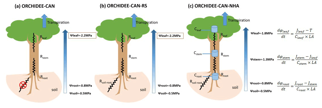
Figure 1Schematic framework for hydraulic architecture in (a) ORCHIDEE-CAN, (b) ORCHIDEE-CAN-RS and (c) ORCHIDEE-CAN-NHA. The framed rectangles represent fixed values during the simulation. In ORCHIDEE-CAN and ORCHIDEE-CAN-RS, Rleaf is related to leaf conductivity and leaf area. Rstem is related to sapwood conductivity that can vary with cavitation and sapwood area. Rroot is related to fine root conductivity and root biomass. In ORCHIDEE-CAN-NHA, transport conductance of each organ is a function of their organ-specific water potential, maximum conductance and water potential when loss of 50 % conductance occurred. Cleaf, Cstem and Croot represent water storage capacitance. Jleaf, Jstem and Jroot are vertical water transport to leaf, stem and root, respectively. LA is total leaf area.
2.1 Model description and simulation protocols
2.1.1 The starting point: ORCHIDEE-CAN r2290
The model version taken as the starting point for development in this study is ORCHIDEE-CAN (r2290), a branch of the ORCHIDEE land surface model. ORCHIDEE is a physical process-based model, which can simulate the energy, water and carbon fluxes between land surfaces and the atmosphere. The SECHIBA module corresponds to faster processes, such as the exchange of water and energy as well as photosynthesis between land and the atmosphere in time intervals of 30 min. The carbon module (STOMATE) simulates soil processes (soil decomposition, heterotrophic respiration, soil organic carbon dynamics) at the 30 min time step and vegetation carbon cycle processes at daily intervals, including carbon allocation, vegetation mortality and recruitment, phenology and litter fall. The development of this branch of the ORCHIDEE model focuses on improving the capability of the ORCHIDEE model to simulate the biogeochemical and biophysical effects of forest management and includes allometric-based allocations of carbon to different pools, a simple plant hydraulic structure (see below) as well as an albedo scheme that in part depends on canopy structure (Naudts et al., 2015). One of its new features is the way the vegetation is discretized; a dynamic canopy structure is simulated by considering a user-defined number of circumference classes (n=20 in this study) and an empirical rule reflecting intra-tree competition that downscales canopy level gross primary productivity (GPP) into the different circumference classes, providing feedback on light interception and mortality through self-thinning. Background mortality comes from the reciprocal of a constant residence time. Climate-based mortality, e.g., from drought, has not been modeled yet using this system.
2.1.2 Hydraulic architecture representation in ORCHIDEE-CAN
In ORCHIDEE-CAN r2290 (Naudts et al., 2015), the representation of water stress is realized through a constraint based on the amount of water that plants can transport from soil to their leaves. This constrained transpiration supply equals the quotient between the water potential gradient from soil to leaves, and a total hydraulic resistance of leaf, stem and root. In this framework, the leaf water potential is fixed to a constant value for each plant functional type (PFT), with a specific minimum value (−2.2 MPa for tropical evergreen forests, Hickler et al., 2006). The soil water potential in the root zone is calculated by adding a tuned scaling factor, accounting for soil–root resistance and other missing processes, to the sum of the soil water potential (calculated from soil moisture and van Genuchten parameters, Van Genuchten, 1980) weighted by a proportion of root mass in each soil layer. Such hard a modulator can sometimes lead to unrealistic soil water potential in the root zone (Joetzjer et al., 2022). The prescribed vegetation distribution is used to constrain this modulator to minimize model bias (Naudts et al., 2015). During the simulation, transpiration is co-limited by the energy budget providing a transpiration demand, and the transpiration water supply limited by transport from soil to leaves. When the potential transpiration constrained by the energy budget is higher than the transpiration supply, real transpiration is limited to the physically plausible water supply. Then the energy budget and photosynthesis-related processes are recalculated. It should be noted that the root- and leaf-resistance parameters in ORCHIDEE-CAN depend only on conductivity and biomass (root mass for root, leaf area index (LAI) for leaf) and do not respond to hydrological conditions directly. Only the stem resistance related to xylem conductivity is dynamic and changes as a function of the soil water potential in the root zone. The schematic framework of the ORCHIDEE-CAN model is illustrated in Fig. 1a. This architecture is not completely mechanistic, given the tuned factor on top of soil water potential, the fixed leaf water potential values and the conductivities affected solely by organ mass. Therefore, further developments of the hydraulic architecture scheme were performed and presented here.
2.1.3 Dynamic root scheme in ORCHIDEE-CAN-RS
To increase the reliability of soil water potential simulations in root zone (Ψsoil-root), Joetzjer et al. (2022) improved this part of the model (flowchart in Fig. 1b, ORCHIDEE-CAN-RS); Ψsoil-rootintegrated Ψsoil in the root zone vertically, i.e., Ψsoil in the root zone is now weighted by the maximum amount of water that can be absorbed by roots in each soil layer (Emax), which depends on a soil-to-root resistance and on a prescribed minimum root water potential (−3 MPa in this study) below which no more water in a given soil layer can be drawn into the plant. The soil-to-root resistance accounts for the water transport path from soil to root surface. With this scheme, the plant will dynamically use deep-layer soil moisture when the surface soil desiccates, so that this process allows the sustenance of more transpiration from deeper layers during the dry periods. Although Joetzjer et al. (2022) solved the problem of tuned modulator imposed on Ψsoil-root by adding a parameterization of the soil-to-root resistance, a more integral mechanistic structure of water transport from soil to leaf remains to be done to enable a dynamic connection between soil and leaf as well as corresponded simulations during drought events. For different cohorts, Ψsoil-root is calculated separately, since we assume taller trees have deeper roots and can reach water stored in deeper layers. For example, we assume that the largest cohort can take water from all 12 soil layers while the smallest cohort can only take water in the shallow layers.
2.1.4 Hydraulic scheme development and implementation in ORCHIDEE-CAN-NHA r7236
Figure 1c presents the schematic diagram of the new hydraulic architecture in ORCHIDEE-CAN-NHA. Besides the water transport driven by vertical water pressure difference, the water flow to/from organ-specific water storage at time t is explicitly modeled based on capacitances and water potential differences between time t and t−1. For each organ, the water supply should meet its water demand. For example, water demand at leaf level is parameterized as the transpiration supply. Water supply to leaf is composed by water transport from stem minus the water charge or plus the discharge from the leaf water storage pool. The water budget of the leaves is calculated first, in order to determine how much water has to be drawn up from the other connected upstream organs. It should be noted that the new hydraulic mechanism is imposed on 20 circumference classes, separately. The detailed description of new mechanistic hydraulic processes is given below.
Water storage calculation
The supply–demand framework is solved at leaf, stem and root, separately. We assume that during the first time step, all water potentials in different organs are the same (Eq. 1). Here, “the first time step” points to the very first 30 min of the simulation. At the first time step, the initial value of Ψl, Ψs, and Ψr are all equal to Ψsoil-root, which is the weighted sum of soil water potential:
Water storage in the different organs is calculated with organ-specific capacitance values (water storage unit: mmol):
where Cleaf is relative leaf capacitance in unit of , L is the leaf dry matter content, Bleaf is the dry leaf biomass and LA is total leaf area. Maximum water storage in leaf (Mleaf,max) is generated by leaf fresh mass minus dry mass; Mleaf,t is leaf water storage at time t.
where Cstem is sapwood capacitance (unit: ), h is tree height in m, Vstem is proportional to the volume of tree stem in m3, γ is the amount of water (mmol) per unit stem volume, which corresponds to the maximum mass of water per stem volume and Msap,max and Msap,t are maximum sapwood water storage and sapwood water storage at time t, respectively. The diameter at breast height (DBH) is D. In the model, we also did a unit transform from kg to mmol:
where ε indicates the amount of water (mmol) stored in per gram of root mass, δ is aboveground wood density, Vroot is root volume, θ is root-to-shoot ratio, Broot is root mass and ρroot is root density. The maximum root water storage and root water storage at time t are Mroot,max and Mroot,t, respectively and Croot is root capacitance (unit: ).
Hydraulic conductance calculation
Hydraulic conductance per unit of leaf area in leaf, sapwood and root at time t (kleaf,t, kstem,t, kroot,t) are calculated with sigmoidal relationships (Pammenter and Van der Willigen, 1998), based on their real-time water potential and a maximum conductance. Water potential is denoted by Ψ50,organ when 50 % conductance lost, and describes the sensitivity of conductance to changes in water potential around Ψ50,organ. An example for how these two shape parameters affect sapwood conductance is shown in Fig. S1 in the Supplement.
where kleaf,t and kleaf,max are leaf conductance at time t and maximum leaf conductance, respectively.
where kstem,t and kstem,max are stem sapwood conductance at time t and maximum stem sapwood conductance, respectively.
where kroot,t and kroot,max are root conductance at time t and maximum root conductance, respectively.
The conductance of the upper part of the tree (leaf plus upper part of stem) and lower part of the tree (lower part of stem plus root) are calculated following Eqs. (14) and (15). These two conductances will be used to calculate the water flow from stem to leaf, and root to stem later, separately. The value 2 in front of kstem,t in each equation denotes that only half of the stem is accounted for in the upper part and trunk part separately. Half of the root length is considered in the trunk part as well. The water transport process is assumed to be similar to electric current, of which the resistance (the reciprocal of hydraulic conductance) should be added up along the water transport path:
Water transport pathway simulation
We assume that for leaves, transpiration supply is based on the water input transported from the stem minus the water charge/discharge from the leaf water storage pool (Eq. 16):
where is the flux of water transported vertically to leaf from stem sapwood (unit: mmol) and is the change in leaf water storage. A positive value of means that the leaf was charged with water during hydraulic recovery, and negative means it was reduced by evapotranspiration (ET). At leaf level, the target is to solve for the leaf water potentials that minimize the difference between potential transpiration demand and supply (Eq. 17):
Similarly, at stem level, the target is to minimize the difference between water demand at stem and water supply to the stem (Eq. 18):
where is the water transported vertically from root to stem and is the change in stem water storage. After solving leaf-level target, is known, which is the water demand at stem.
At root level, the target is to minimize the difference between water demand at root and water supply to root (Eq. 19):
where is the water transported from soil in root zone to root and is the change in root water storage. After solving stem-level target, is known, which is the water demand at root. The detailed calculations of these water flow variables are explained below in the order of leaf, stem and root.
Thus, water potentials are solved to let the water supply be equal to water demand at each organ. In the model, the HYBRD1 function from Minpack package in Fortran is used, which seeks a zero of N nonlinear equations in N variables. The evaluated function is the difference between water supply and water demand at each organ level. This function iteratively minimizes the absolute value of the evaluated function. The initial estimate of the solution vector is quite important and comes from the water potential at the last time step. For example, the initial estimate for leaf water potential at time step t that will be used in the formula is the stem water potential at time step t−1.
a. Leaf transport
The water movement into the leaf through the hydraulic pathway is calculated as follows:
where a positive means an increase in leaf water storage and vice versa and indicates how much water potential gradient is needed to pull water against gravity up to the height (h) of the tree from the position of tree height (middle of stem).
We calculate and using an optimization procedure, i.e., we start by assuming and progressively decrease until the difference between leaf water supply and demand is close to zero (Eq. 22). Leaf water potential is solved using the HYBRD1 function (see above). The tolerance is 0.00001 MPa. When the relative error between two consecutive iterates is below the tolerance, the calculation routine is terminated:
where PTdemand (potential transpiration demand) is related to stomatal conductance, vapor pressure deficit (VPD) and total leaf area (Eq. 23), where stomatal conductance varies with Ψleaf (Eq. 24):
where gs, gmax and gmin are in the unit of , VPD is in the unit of kPa and LA is the total leaf area.
The standard atmospheric pressure is denoted by P (101.3 kPa). The aim of this gs model is to let gs vary, following dynamics of leaf water potential in the sigmoidal function, then gs can be coupled into the plant water transport system via the transpiration supply. Meanwhile, the gs is assured to be close to 0 in the night, mediated by the radiation-related variable () and L and Lk are parameters specifying the strength of short-wave radiation limitation on stomatal conductance. Minimum leaf water potential in this study is set to −3.0 MPa to avoid unrealistic values (Fisher et al., 2006).
We verified that our simulated gs with the parameter values from Table A2 are of similar magnitude than in the soil–plant–atmosphere (SPA) model of Fisher et al. (2007) at Caxiuanã, which was developed independently from ORCHIDEE (Fig. S2). The gs in the SPA model is obtained by maximizing the marginal carbon gain of stomatal openness (intrinsic water use efficiency). Further, in order to show that our model parameters can be used to simulate gs at other rainforest sites, we collected gs observations (at leaf scale) from two rainforests in French Guiana and Peru from Lin et al. (2015) and tested our model against these observations. Figure S3 shows that our simulated gs values fall in the range observed at these two sites.
b. Stem transport
Next, we know that the water demand at stem is the amount of water transported from stem to leaf, . We can now use the same procedure to calculate the that produces the expected , and how much of that transport is from storage and from the roots through the vertical hydraulic pathway:
where is the water supply to stem and is the water demand at stem. We then solved the to minimize the difference between and (Eqs. 27 and 28).
c. Root transport
The same procedure is also carried out for root. The total flow out of the root is equal to . We calculate root water transport according to the following equations:
where is the water demand at root and is the water supply to root. We then solved the to minimize the difference between and (Eqs. 31 and 32). The “2” in Eq. (29) means half of the root is accounted for () here since the other half of the root is considered in ktrunk,t.
We assume that water does not travel in reverse, leaving the roots and going into the soil. We also impose a limit on vertical water flow to non-negative values.
Update water storage pools
After the simulation of water transport, we use the Wt+1 values to update the water storage in each organ:
All of the above calculation processes are carried out for 20 circumference classes, separately. The parameters used in the new hydraulic architecture are summarized in Table A2. We did some sensitivity tests by attempting different value combinations of parameters within a range of records in literature, such as degree of vulnerability, Ψ50 and degree of sensitivity, a (shape parameter), as shown in Fig. S4. Parameters set that can better capture the observed variation of drought-induced tree mortality (especially the higher tree mortality rate in larger cohorts) was chosen. We do not aim for a perfect match between model output and observation to avoid the overfit issue during the generalization of the model.
2.1.5 Parameterization of tree mortality related to drought
Since trees can endure drought conditions and do not die after 1 or 2 d of low stem water potential or water shortage (Brodribb et al., 2020), we defined an exposure threshold desiccation time to trigger mortality. Continuous exposure to a high percentage loss of conductance (PLC) forebodes tree mortality, therefore a decision rule was set with two empirical parameters, a drought mortality exposure threshold (in days) and a mortality fraction of trees each time (in % of all trees that die). When the PLC > 50 % condition lasts for more than 15 continuous days, we assume that a fraction of 0.3 % of all the trees in each size cohort are killed. These two parameters are tuned according to the observed annual mortality rates. It should be noted that a cohort model represents all the trees in a grid cell as one average individual, thus an absolute mortality threshold would kill them all on the same day. Hence we impose a fractional mortality to capture the variability in mortality drivers and processes within each cohort. We also consider that a very short wetting break during a drought condition would not necessarily act to reverse embolism and thus the tree's exposure to mortality. Here, the minimum threshold for a continuous wetting break (PLC < 50 %) to reset the exposure to zero is set to 5 d. The annual mortality rate equals to the number of dead trees per year divided by the number of trees alive in the beginning of this year.
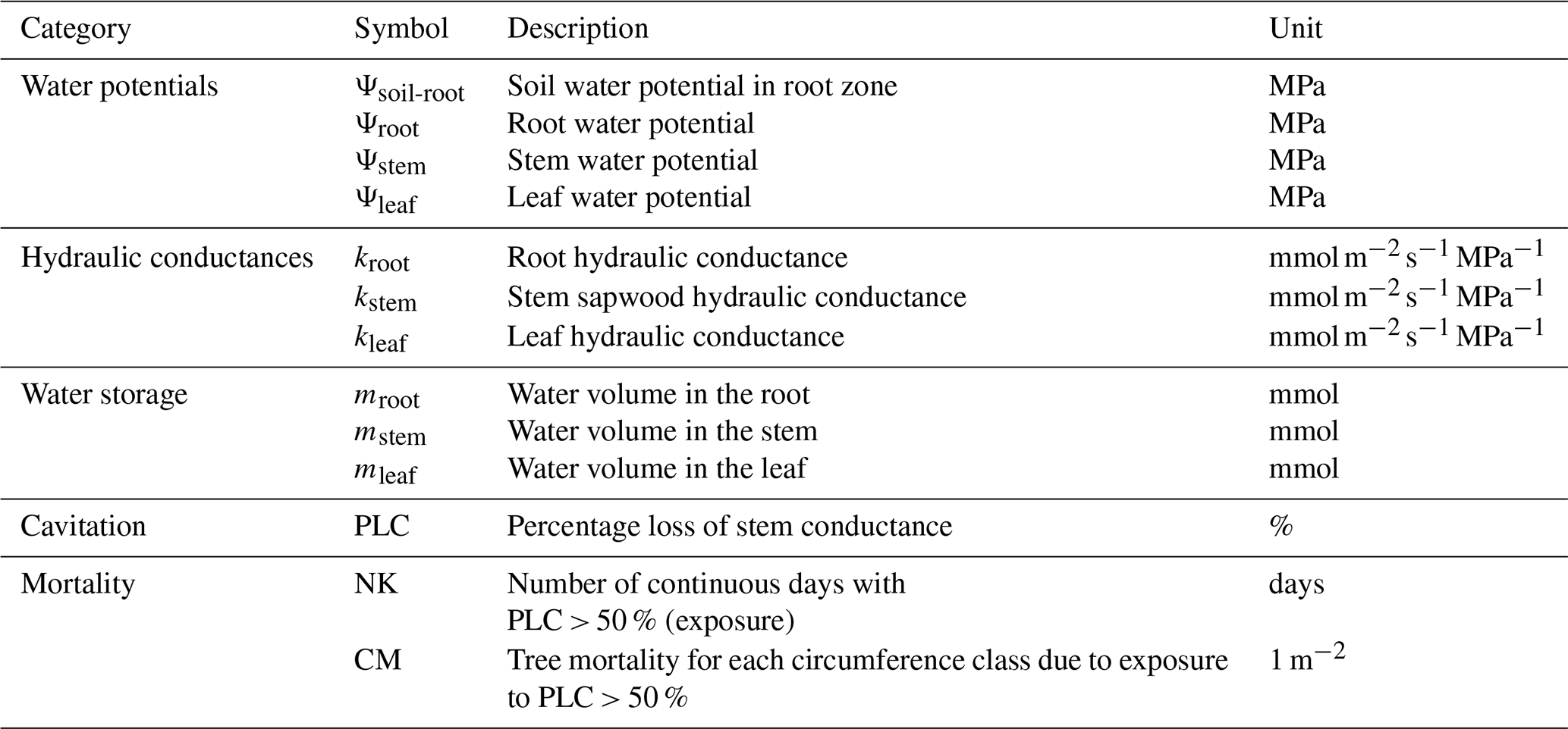
Finally, following ORCHIDEE-CAN-RS, the recruitment rate is determined by LAI (Joetzjer et al., 2022). LAI is determined by leaf mass, which is regulated by the leaf growth, leaf turnover and leaf loss due to drought-induced tree mortality. When LAI decreases during drought, the recruitment rate will increase correspondingly since recruitment is parameterized as a function of LAI. The new outputs from ORCHIDEE-CAN-NHA are listed in Table A3.
2.2 Biomass growth and loss calculation
As ORCHIDEE does not account for biogenic volatile organic compound (BVOC) emissions, root exudation and C-subsidies to mycorrhizae, biomass growth is simulated as the residual of GPP minus autotrophic respiration. Biomass loss comes from three processes in ORCHIDEE: turnover (loss of leaves and fine roots), self-thinning and climate-induced mortality, i.e., drought for this study. It should be noted that, in ORCHIDEE-CAN, when the number of individuals falls below a parameterized threshold, self-thinning does not happen and individuals grow without competing with each other. This calculation process is the same among three different model versions.
2.3 Site description
The study site is a tropical lowland rainforest located in the Caxiuanã National forest, state of Para, northeast of Brazil (1∘43′ S, 51∘27′ W). Annual rainfall in this site is 2000–2500 mm with a dry season spanning from July to November (monthly rainfall < 100 mm). There are two experiments, which were carried out since the beginning of 2001. A throughfall exclusion experiment (TFE) started at the end of the dry season in 2001, where 50 % of canopy throughfall is excluded by plastic roof at the height of 1–2 m above the ground (Fisher et al., 2007; Meir et al., 2018). It is 1 ha in size. Another 1 ha control plot is also set without any manipulation. Here, the observation data we used extend to 2008 at most due to data-access issues, but these experiments are still running.
Table 1Collected observation data used for validation of process-based model simulation.
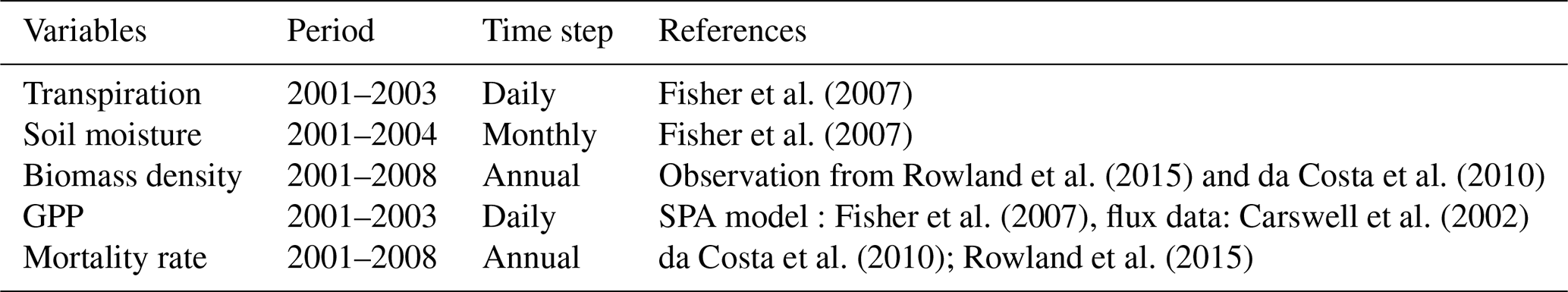
From published literature (Carswell et al., 2002; da Costa et al., 2010; Fisher et al., 2007; Rowland et al., 2015), we collected observation data as validation for model simulation, including transpiration data, soil moisture data, annual mortality rate, annual biomass density, and GPP (Table 1). We also used output from the SPA (soil–plant–atmosphere) model with parameters measured for the Caxiuanã experiment. The SPA model is a multilayer soil–plant–atmosphere transfer model, which has been parameterized upon such drought-affected ecosystems (Fisher et al., 2007). We included simulated GPP output from SPA for model comparison under TFE since eddy covariance flux measurements can only be used in model–data comparison under control (CTL).
2.4 Simulation protocols
We performed three simulations at site-level for Caxiuanã to compare the hydraulic architecture from each model version. Specifically, we tested the model performance under two setups, the control (CTL) and the throughfall exclusion experiment (TFE). In the model, TFE is reproduced by keeping only 50 % of the rainfall of CTL with all else being the same as CTL (Fisher et al., 2007). It should be noted that such a rainfall cut is a simplification, since in reality, a plastic panel is used to exclude 50 % of throughfall. We ran 250 year spin-ups by cycling climate-forcing data over 2001 to 2008 with constant CO2 concentration of 380 ppm to get the preliminary state of carbon pools and water flow at the beginning of 2001. The meteorological forcing is at 30 min time steps. The meteorological data every 30 min are measured using an automatic weather station located at the top (51.5 m) of a tower 1 km from the experimental plot. The simulation was run offline without coupling with a climate model. Two former model versions and our new developments are integrated as below. We compared ORCHIDEE-CAN-RS and ORCHIDEE-CAN-NHA to see the improvements brought by the new hydraulic architecture. It should be noted that all three of these simulations are realized through several flags to switch on/off some functionality:
-
ORCHIDEE-CAN with the original simple hydraulic module setup,
-
ORCHIDEE-CAN-RS, which adds a new dynamic soil–root scheme on top of (1),
-
ORCHIDEE-CAN-NHA, with the new mechanistic hydraulics on top of (2).
2.5 Statistical tools
We used the R programming environment and statistical packages (version 3.5.0; R Core Team, 2019) for all data processing and analysis. Package ncdf4 v1.17 (Pierce, 2019) is used to handle files in NetCDF format from model outputs. Package fields v10.3 (Nychka D, 2020) is used in water potential plotting.
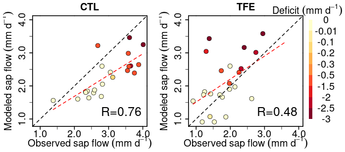
Figure 2Modeled (ORCHIDEE-CAN-NHA) vs. observed sap flow (monthly average values are displayed). The color of points indicates water deficit (negative difference between precipitation and evapotranspiration) with darker color meaning more severe water deficit. The dashed black line is the 1:1 line. The dashed red line is the best fit between modeled and observed sap flow.
3.1 Model evaluation against observation
3.1.1 Evapotranspiration and soil moisture
Under the CTL condition, the model developed here (ORCHIDEE-CAN-NHA) agreed well with the sap-flow observations from well-watered periods but underestimated sap flow in the dry season. The dry-season points in Fig. 2 are those with a water deficit of up to −3 mm d−1 (monthly precipitation below evapotranspiration). Regressing modeled transpiration with sap-flow observations, we found that the model better represents the month-to-month seasonal variability under CTL than TFE (R=0.76 in CTL v.s. R=0.48 in TFE). Under the TFE condition, the model overestimated transpiration in both the wet and dry seasons, with a positive bias increasing at water deficits typically below −2 mm d−1 (Fig. 2). Simulation by ORCHIDEE-CAN-RS also showed such a positive bias (Fig. S5). This positive model bias was mainly contributed by the simulation in 2002 when the TFE experiment was installed by the end of 2001. The transpiration supply did not show water limitation on transpiration under TFE until the end of the dry season in 2002 (Fig. S6). The simulated transpiration could be limited by water supply (water limitation) or water demand (energy limitation). Under CTL, there is almost no water limitation, even in the dry season. The underestimated sap flow can be due to the fact that the model tends to underestimate the sensitivity to VPD increase in the dry season. Under TFE, there is water supply limitation. The possible reasons for such overestimation under TFE can be that the sensitivity of water supply to drop in soil moisture is underestimated or the too-slow soil water drainage in our model setup is relative to that in reality (Kennedy et al., 2019).
In terms of comparison on transpiration (Table S1 in the Supplement), under CTL, the correlation coefficient with the observation is similar among the three model versions (0.71–0.76), although there is indeed a bit increase in other error metrics in ORCHIDEE-CAN-NHA, like the root mean square error (RMSE) and mean absolute percentage error (MAPE). The ORCHIDEE-CAN-NHA performs better in water-stress conditions (under TFE) in aspects of these error metrics, but shows a bit lower correlation with observation than the other two versions.
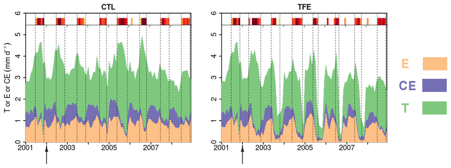
Figure 3Modeled (ORCHIDEE-CAN-NHA) daily soil evaporation (E), canopy evaporation (CE) and transpiration (T) during 2001–2008. The arrows point to the start of TFE at the beginning of 2002. The inserted shaded red bars denote the periods with water deficits during the simulation period, following the same color scale as Fig. 2.
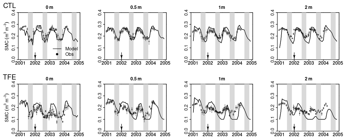
Figure 4Modeled (ORCHIDEE-CAN-NHA, black line) vs. observed (black dots) volumetric soil moisture content (SMC) at different depths. Due to the limited time duration of observation data, we only show the modeled SMC during 2001–2004. The shaded gray vertical area indicates the dry seasons from July to November.
The partitioning of evapotranspiration (ET) was compared between CTL and TFE. Under the CTL condition, the modeled partitioning of ET into transpiration (T), intercepted canopy water or dew re-evaporation (CE), and bare soil evaporation (E) is shown in Fig. S7, with the ratio () being around 0.57 in the wet season, and 0.74 in the dry season. Under TFE, the difference of between the dry and the wet seasons increased (wet: 0.58 vs. dry: 0.82). Specifically, under CTL, the daily mean transpiration can reach more than 4 mm d−1 and soil evaporation accounted for 29 % of the total ET in the wet season. The magnitude of transpiration increased by 51 % in the dry season (range: 22 %–71 %) compared to that in the wet season under CTL, which is similar to the observations (+44 % in Fisher et al., 2007), due to higher energy supply and non-water limiting conditions. This indicated that normal conditions at this site are not very strongly limited by soil moisture during the dry season, despite recurrent deficits, as shown by the red bars on the top of Fig. 3. Nevertheless, under TFE, the transpiration was lower than in CTL and encountered emerging water-supply-induced limitation in the dry season, with of 1.12 over 2002–2008 (minimum can be 0.60 in 2005) (Fig. 3). Soil evaporation also decreased a lot under TFE from the wet to the dry season, and the ratio () was halved from the wet to the dry season, especially in the years 2005, 2006 and 2007, when annual rainfall was relatively lower.
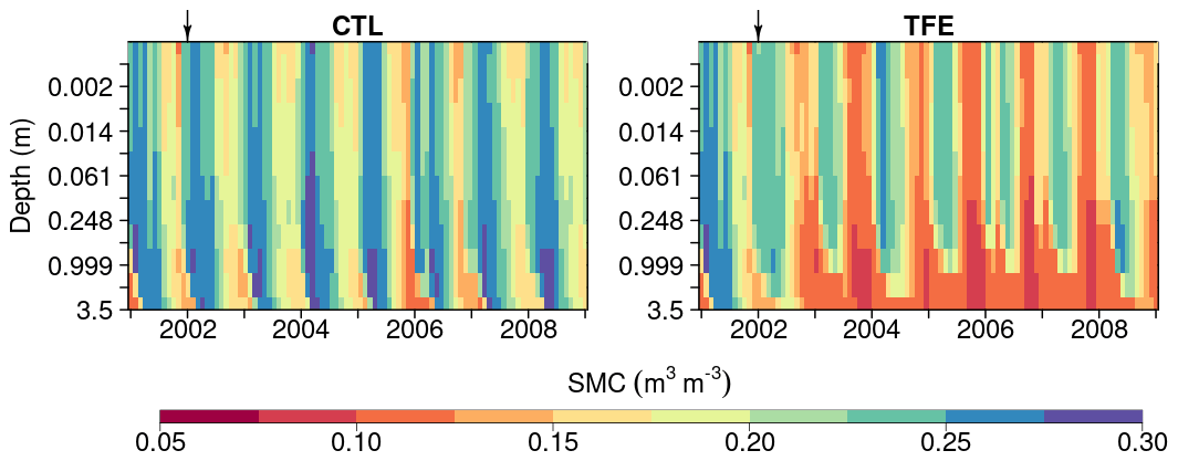
Figure 5Soil moisture content (SMC) simulated by ORCHIDEE-CAN-NHA during 2001–2008 under CTL and TFE. It should be noted that the 12 soil layers have different thicknesses and here we show the SMC in the same depth interval to present the change in SMC in top layers clearly.
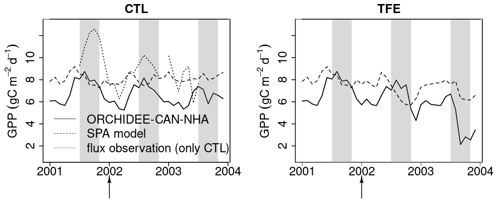
Figure 6Modeled (ORCHIDEE-CAN-NHA) vs. observed/modeled monthly mean GPP. The control model is compared to flux-tower observations (Carswell et al., 2002). In the case of TFE, as no observation is available, the locally calibrated SPA model is used. Due to GPP, flux observation is unrealistically low at the start of 2001 (< 5 ), we only keep flux data after mid-2001. The shaded gray vertical area indicates the dry season from July to November.
We next examined the model performance (ORCHIDEE-CAN-NHA) for reproducing the soil moisture dynamics during the observation period between 2001 and 2004. Soil moisture content (SMC) featured a pronounced seasonal decrease between the wet and dry periods under CTL and TFE (Fig. 4). Under CTL, in the surface soil, the model produced a small underestimation of SMC in both wet and dry seasons compared to observation. With increasing depth in the soil, this negative difference between modeled and observed SMC became more pronounced in the dry season (Fig. 4). Under TFE, a similar negative difference also appeared in the dry season only, while a positive difference appeared in the wet period. Besides, under TFE, the modeled SMC was however always lower than for CTL in the surface layer, and became even more depleted in the deeper layer with the dynamic soil–root scheme, even in the wet season (Fig. 5), because this scheme shifts root uptake from surface to deep layers when the surface dries out compared to the simulation of ORCHIDEE-CAN (Fig. S8). The SMC at each layer is influenced by infiltration, evaporation, transpiration and drainage. The amount of water that can be absorbed from each layer (η) is determined by its water potential and also soil–root resistance. Soil water potential decreases with soil depth while soil–root resistance becomes much smaller with soil depth as well. Therefore, η does not change monotonically with soil depth. For example, during the wet season in 2005 under TFE, η in the deeper soil layer is higher than that in the top layer, while in the dry season, η in the deeper soil layer can decrease to almost 0 when the water supply mainly comes from the shallower layer. In year 2004, even in the dry season, lower soil layers can contribute a lot to water uptake (Fig. S9).
3.1.2 Carbon fluxes
The GPP simulation outputs had a similar seasonality under CTL among all model versions (Fig. S10 in the Supplement). All simulations showed higher GPP in the dry season compared to the wet season under CTL (also in eddy covariance, Carswell et al., 2002) (Table S2). When we compared GPP against the SPA model results from Fisher et al. (2007) that were calibrated to best-fit site-level observations, and against flux observation, we found that modeled GPP in ORCHIDEE-CAN-NHA showed a larger seasonal amplitude than that of SPA but with a similar phase (Fig. 6). The GPP from ORCHIDEE-CAN-NHA presents a 1.1 difference between wet and dry seasons, which is similar to the two previous versions. The GPP seasonality from eddy covariance data was also in agreement with the simulation from ORCHIDEE-CAN-NHA, with a peak in the middle of the dry season. In contrast, the SPA-modeled GPP decreased right from the start of the dry season. We found that the impact of the TFE condition on modeled GPP was relatively small during the wet season, with a difference less than 10 % in comparison with CTL (see Fig. S10 for the two other versions). On the other hand, the impact of TFE during the dry season led to a pronounced decrease of GPP, like in the SPA model. In ORCHIDEE-CAN-NHA, GPP decreased only at the end of the dry season under TFE while in SPA, it decreased from the beginning (Fig. 6). Only after 2 years of drought, ORCHIDEE-CAN-NHA simulated an early decrease of GPP at the beginning of the dry season, and thus became consistent with SPA (Fig. 6). The dry season GPP increase is also found in the other two model versions, despite a bit difference in the magnitude. In the SPA model, GPP is simulated using the FvCB model regulated by optimization of intrinsic water use efficiency, in which the optimization target is (A is assimilation, gs is stomatal conductance), not accounting for VPD. So the magnitude of the GPP variation would not be too high. In ORCHIDEE-CAN-NHA that we used here, larger seasonal amplitude of the modeled GPP, especially the low GPP in the dry season under TFE, is due to higher water limitation imposed from our hydraulic architecture.
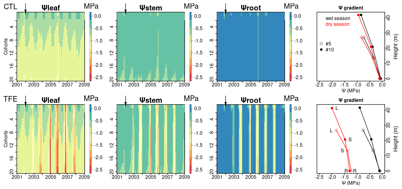
Figure 7Ψleaf, Ψstem, and Ψroot simulated by ORCHIDEE-CAN-NHA. Water potential gradients of two cohorts (#5, #10) are shown as an example (May 2005 as the wet season and November 2005 as the dry season). Here, the cohort refers to the circumference class (mean height of #5 and #10 are 19 and 35 m, respectively). The water potential gradient is composed by Ψleaf (labeled as L), Ψstem (labeled as S) and Ψroot (labeled as R). The heights of Ψleaf and Ψstem correspond to tree height and half of tree height, respectively.
3.2 Simulated water potential gradients along the soil-to-leaf continuum
With the mechanistic hydraulic architecture of ORCHIDEE-CAN-NHA, the dynamic water potential at leaf, stem and root levels were modeled and compared with observations (Fig. S11 in the Supplement). The diurnal cycle of Ψleaf was comparable between model and observations, although the modeled Ψleaf was less negative than the observation at noon (Fig. S11). The lowest water potential was simulated in the leaf, followed by the stem, as expected. There was clear seasonal variability between the wet and dry periods, especially under TFE conditions (Fig. 7). Under CTL, the water potential vertical negative gradient between leaf and root was similar between the wet and the dry seasons (−0.79 MPa in the wet season and −0.84 MPa in the dry season for tree cohort #10 that is in diameter of 1.15 m; for the cohorts description see the Methods section); the minimum monthly mean Ψleaf, Ψstem and Ψroot were −1.3, −1.0 and −0.8 MPa in the dry season, respectively. Under TFE, Ψleaf, Ψstem and Ψroot were prominently more negative during the dry season (−2.5, −1.9, −1.7 MPa, respectively) and the range of water potential gradients between stem and root in the dry season became a bit narrower than that in the wet season, which reflected the fact that the water flow from vertical transport is limited. With regard to the change of water storage, leaf water storage decreased continuously from the wet to dry seasons but did not approach depletion of water storage (Fig. S12 in the Supplement). In year 2005, Ψleaf in the dry season (dry season rainfall is minimum) reached its minimum during the entire simulation period under TFE. We can see that at leaf and stem levels, Ψleaf and Ψstem decreased slightly with the size of cohorts and they were a bit more negative in larger (taller) cohorts correspondingly (Figs. 7 and S13 in the Supplement). Taller trees have a longer water transport path, which means greater gravitational potential energy is needed to pull water upward (Eq. 20). Thus, more negative Ψ values were expected in the circumference classes with higher trees; Ψsoil-root did not show too much variation among different cohorts (Fig. S14 in the Supplement). Then the leaf water potential difference among cohorts is mainly contributed by the height effect, which is about −0.1 MPa 10 m−1.
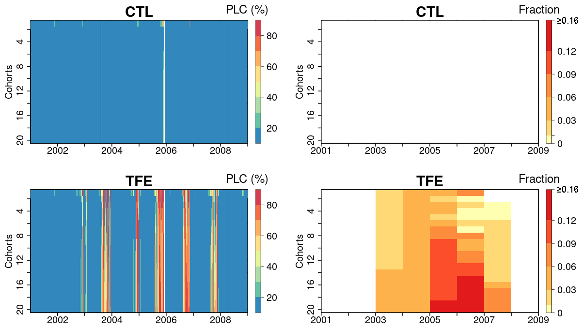
Figure 8Percentage loss of daily stem conductance (PLC) (left) and tree mortality fraction simulated by ORCHIDEE-CAN-NHA (right). The vertical axis is for the index of 20 tree cohorts represented in the model, a larger index indicating taller trees (see Table S4 for tree height and diameter in each cohort). Tree mortality fraction per year is calculated by totaling the number of dead trees in each year and dividing it by the tree density on the first day of each year.
3.3 Simulated hydraulic failure
Here, we used the simulated PLC in stem sapwood as an indicator of tree hydraulic failure. Under CTL, the PLC remained lower than 50 %, even in dry seasons, due to weak water limitation (see soil moisture deficits in Fig. 4 and water potential gradients in Fig. 7). Under TFE, the PLC did not reach above 50 % in wet seasons, but in dry seasons, it increased to more than 80 %, especially in the (abnormally dry) year 2005 (Fig. 8). Under TFE, the number of days with a PLC above 50 % were 12 d, 63 d in years 2002 and 2003, respectively, and reached up to 84 d in year 2005 (cohort #10). Besides its seasonal variability, the PLC also moderately increased with the size of cohorts, denoting more severe water stress in larger/taller cohorts (Fig. S15 in the Supplement).
Next, we looked at the two variables defined to link PLC with mortality in the model: the PLC mortality exposure threshold and the mortality fraction per day of exposure (see Methods section). The mortality exposure threshold represents a maximum tolerable drought duration for trees before a fraction of them die. In this study, this mortality threshold is set to consecutive 15 d when the PLC stays above 50 %. The mortality fraction is set to a death rate of 0.3 % during each day of the exposure period (no preferential rule is imposed for small or large trees). In the absence of any measurement, the values of these two mortality-triggering variables were calibrated to reproduce the observed mortality in the TFE experiment. We estimated the mortality fraction by totaling the dead trees in each year and dividing this number by the initial tree density in each year. With this scheme, estimated drought-induced tree mortality rates were shown in Fig. 8. The model simulated that more than 10 % of trees in larger cohorts (#12 to #20) would be killed by the dry conditions in 2005 (Fig. 8), which was a bit higher than the 7 % of mortality observed in the experiment. Figures S16 and S17 in the Supplement present that a smaller cohort (#5 here) shows somewhat larger variation in water potential dynamics and corresponding PLC, which indicates that an adequate cumulated drought exposure occurs less frequently than in larger cohorts (#20 here). Thus, the higher annual tree mortality rate is found in larger cohorts (Fig. 8).
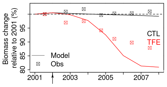
Figure 9Tree biomass change simulated by model after mortality being triggered. The squares in the plot denote the observation. Biomass change relative to 2001 is calculated by dividing biomass during 2002–2008 by biomass in 2001.
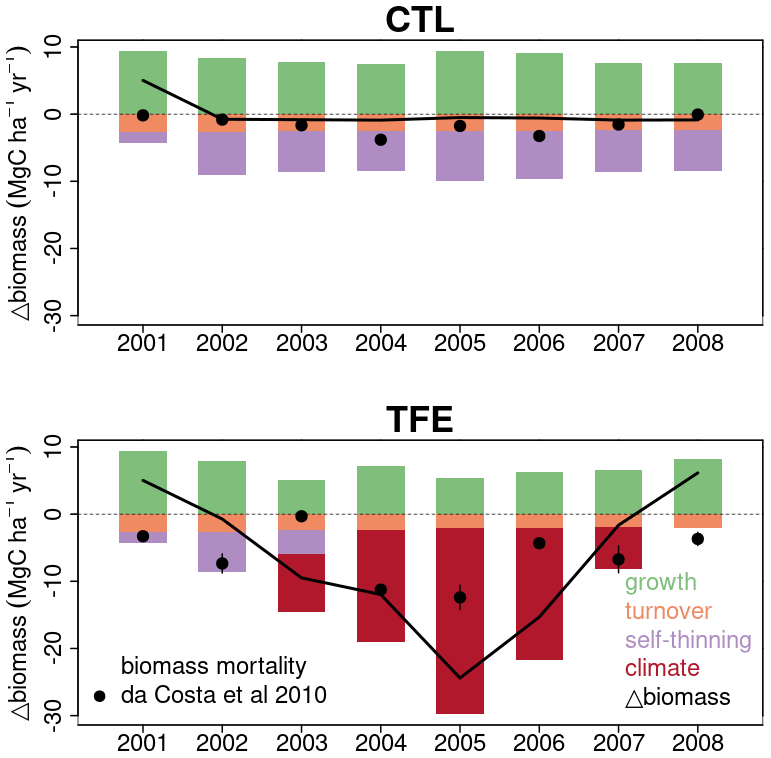
Figure 10Simulated components of biomass change and observed net biomass change during 2001–2008. The observed net biomass change data in each year from da Costa et al. (2010) are plotted as black dot. The black line shows the net change of simulated biomass by ORCHIDEE-CAN-NHA.
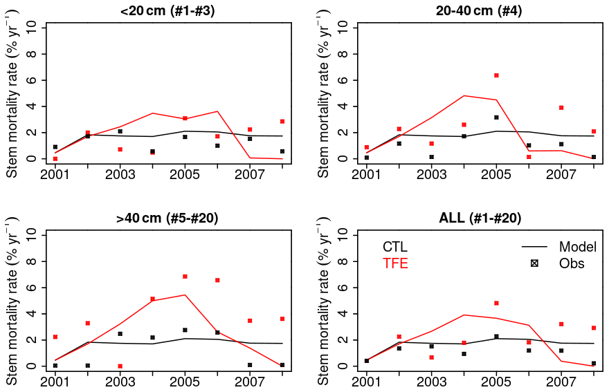
Figure 11Annual stem mortality rates during the study period (2001–2008). All 20 cohorts have been aggregated to three classes according to DBH (< 20, 20–40, > 40 cm). The value in brackets in the title of each panel corresponds to the cohort numbers falling in the class.
The model simulation (ORCHIDEE-CAN-NHA) produced a reasonable (but slightly too large) biomass mortality under TFE during 2002–2008 (Figs. 9 and S18 in the Supplement), with a modeled biomass loss (∼ 67 Mg C ha−1, ∼ 19 % of biomass in 2001) being a bit larger than the observation (∼ 30 Mg C ha−1, ∼ 12 % of biomass in 2001). The other two previous model versions cannot reproduce the comparable drought-induced biomass loss (Table S3). Figure 10 showed that under CTL, the biomass loss due to self-thinning and turnover is almost compensated by the biomass growth and recruitment. Under TFE, self-thinning only existed in the years before 2004 according to the model, because a drop of tree density was induced by preceding drought mortality in 2003, which suppressed the competition between trees in the model afterwards. The gain of biomass (labeled as “growth” in green in Fig. 10) also decreased under TFE in comparison with CTL. Moreover, when we grouped the mortality rate simulated for 20 cohorts into three classes according to their DBH (< 20, 20–40 and > 40 cm), we can further evaluate the model performance (Fig. 11). Under CTL, the model produced a higher mortality rate (1.7 %) than the observation (2001:2008 mean: 1.1 %–1.3 %) in three classes. In other words, the modeled self-thinning rate was probably higher than that in reality since the mortality rate observed was only 0.4 % in year 2001. Under TFE, the model performed differently for each size class. For the small-sized class with DBH < 20 cm, the model underestimated the mortality rate compared to observations after 2006. For the medium-sized class (DBH: 20–40 cm), the modeled mortality rate was comparable with observations in year 2001, 2002 and 2006. For the large-sized class group, the model can successfully estimate the large mortality observed in situ from 2004 to 2005. Overall, the averaged mortality rate was comparable between observation and model simulation. The model–observation gap in year 2005, 3.7 % in model simulation vs. 4.8 % in observation, may be due to modeled underestimation in a medium-sized group and large-sized group (Fig. 11).
Finally, we tested the performance of our hydraulic failure–mortality submodel at another TFE site in the Amazon, from the Tapajos site (Nepstad et al., 2007). At this site, TFE only happened in the wet season between 2000 and 2003, with an exclusion of almost 50 % rainfall. Figure S19 in the Supplement shows that our model can capture the observed phenomenon of a higher mortality rate found at Tapajos, especially in trees with a diameter > 30 cm, although the modeled mortality rate is lower than that in the field measurement. Our model also simulates the net biomass increase at Tapajos under CTL and the great biomass loss under TFE. The two parameters of our hydraulic failure–mortality model (drought exposure threshold and mortality fraction each day upon exceeding the threshold), which are not directly observable, were effectively calibrated at Caxiuanã, but the model is also successfully evaluated at Tapajos site. Given the complexity of drought–mortality relationships which lack a unified theory, this shows high performances for the new parameterization we proposed in the study.
4.1 Model improvements by new parameterizations of hydraulic transport
The original ORCHIDEE-CAN model included a limit from transpiration supply based on water transport and resistances along a water potential gradient (Naudts et al., 2015). Nonetheless, the constant value assumed for Ψleaf, the lack of a dynamic simulation of Ψstem and Ψroot and conductivities limit the mechanistic basis of the approach. To make a step forward, the new hydraulic module presented here tracks the water flow continuum from the soil to the atmosphere. The water potentials Ψleaf, Ψstem and Ψroot are updated at each 30 min time step, based upon a supply–demand framework of minimization of the difference between water demand and water supply at organ level. Besides improvements in modeling the processes of vertical water transport, our hydraulic module also considers the tissue water storage and the dynamics of water flow between different organs, both of which are bounded by the capacitance and water volume. The water storage capacity can affect the water potential and determine the tolerable duration of desiccation before severe water potentials are reached (Gleason et al., 2014). For example, in the model, stem sapwood water storage can be discharged under CTL during both the wet and dry periods, and this contribution can be larger than that from vertical water flow. In contrast, under TFE, the stem sapwood water pool is not always refilled overnight in the dry season (Fig. S20 in the Supplement). Martinez-Vilalta et al. (2019) also found that a more explicit consideration of water pools helps advance the monitoring and prediction of mortality risk, although more experimental evidence is required for verifying the relationship between relative water content and mortality probability.
Besides the capacity of each organ, stem hydraulic safety indicators like water potential, at which 50 % of stem conductance is lost (Ψ50), can be modeled directly and used as an indicator of tree responses to drought events. This variable influences the maximum drought exposure threshold proposed in our model, which varies among specific tree species, tree size and different growth conditions (Blackman et al., 2016). In a previous study at this site, Rowland et al. (2015) found that vulnerable and resistant genera have contrasting vulnerability to hydraulic deterioration. Vulnerable trees with larger DBH displayed higher conductivity loss under experimental drought and less negative Ψ50. However, in a more recent study with much more field data in Bittencourt et al. (2020), the variability of hydraulic traits among species is also evident and the importance of particular hyper-dominant species also becomes notable in affecting the overall species and size patterns. Naudts et al. (2015) related stem conductivity to Ψsoil-root with Ψ50 and another shape parameter as an adjustment. In our model, we built sigmoidal relationships between conductance and Ψstem, of which the slope parameter assesses the sensitivity of conductance loss to decline in water potential that can correspond to different plant water-regulation strategies. Through involving trait-related parameters, our model could be used to reflect isohydric or anisohydric patterns, although these two parameters are challenging to calibrate for highly diverse tropical forests (e.g., Maréchaux et al., 2015).
Recently, there has been expansion in the availability of the hydraulic parameters for tropics, but mainly for xylem and leaves. Although the sensitivity analysis of the supply–demand theory in Sperry et al. (2016) suggested that the usage of the single-stem vulnerability curve would not bring more error to transpiration than the true segmented mode (i.e., separate leaf, stem and root curves) as long as the leaf/stem Ψ50 and root/stem Ψ50 is closer to 1, our study included vulnerability segmentation of leaf, stem and root to facilitate the coherent representation of the soil–root–stem–leaf continuum. Besides, the possible context-dependent trait coordination also needs to be noticed in parameterizing models (Maréchaux et al., 2020), e.g., the relationship between leaf turgor loss point and leaf area, which will benefit the diversity in vegetation models.
With water transport from the vertical gradient of potentials and changes in water storage, ORCHIDEE-CAN-NHA produced dynamic and reasonable water potentials (Fig. S11) and conductance at leaf, stem and root levels. Based on the improved hydraulic architecture, we implemented an empirical algorithm that assumes that a fixed fraction of trees will die after 15 d of continuous sustained drought exposure with PLC > 50 %. Combinations of these two parameters of drought exposure threshold and mortality fraction each time could also be adapted to diverse plant traits to match mortality rates across different sites, coping with adverse conditions, e.g., tree size, different isohydric and anisohydric behaviors of stomatal regulation upon varying water status (McDowell et al., 2008). Therefore, these two parameters would need to be calibrated upon data suited to different conditions. For example, Esquivel-Muelbert et al. (2017) found that wet-affiliated genera tend to show higher drought-induced mortality than dry-affiliated ones. Assigning higher mortality fraction for wet-affiliated genera under such conditions can be a solution to test different levels of mortality fraction parameters.
The supply–demand framework in our model also draws on Sperry et al. (2016) that the empirical expression of each continuum component, e.g., stomatal conductance and hydraulic conductivities from the vulnerability curve, is applied. There are also similarities between our hydraulic structure and that of Xu et al. (2016) in aspects that both vertical water flow and water storage capacity in leaf and stem are accounted for in the modeling process of water supply and demand. The major differences from the model of Xu et al. (2016) are that our model uses potential water demand (rather than the real transpiration) as the leaf-level demand instead and also refines the water transport from soil–root–stem, thus the water potential of each organ in the continuum is solved.
The earlier hydraulic models like SPA and that of Xu et al. (2016) indeed proposed the simulation framework of water flow and water potential following Darcy's law; however, a full segmentation of the hydraulic system including water flow and water storage change of leaves, stem and root are still not completely solved (i.e., the root part was missing in Xu et al., 2016). Our hydraulic architecture refines the segmentation of plant hydraulics of leaves, stem and root, separately, of which the hydraulic conductance varies with water potential value following the sigmoidal relationship. Meanwhile, the water capacitance is considered as well to account for the variation in water storage. The hydraulic models like SPA and that of Xu et al. (2016), lack either the full segmentation or the consideration of contribution of each water storage pool (SPA model only used canopy capacitance). Our model also extends one step further to link the hydraulic failure measured by PLC to the tree mortality rate via an empirical model composed of two parameters: drought exposure threshold (number of continuous days under water stress), and tree mortality fraction upon each tree mortality event. This tree mortality submodel accounts for the cumulative drought effects, which can adapt to different drought strengths and drought frequencies. Therefore, our hydraulic model with tree mortality scheme improves the hydraulic segmentation simulation and also paves a new way of linking hydraulic failure to tree mortality. Admittedly, weakness does exist in our model, e.g., parameter retrieval can be further realized through data assimilation that use more benchmarking (see below). More optimization paradigms can be integrated into our model, which would benefit the parameterization process.
4.2 Possible factors affecting tree mortality
Our model simulations showed that larger trees suffer more severe water stress with higher PLC (Fig. 8) and that the mortality fraction is consequently the highest in groups with DBH > 40 cm. This uses the theory that longer, vertical water transport pathways in taller trees can intensify the height-dependent hydraulic limitation (Grote et al., 2016) and site-level experimental evidence (Rowland et al., 2015). Such size-regulated mortality has also been corroborated by Bennett et al. (2015). Hendrik and Maxime (2017) summarized that drought can be more detrimental to growth and mortality rates of larger trees. Klos et al. (2009) also found that older and denser stands are more susceptible to drought damage, but that the mortality–height relationship can also be relaxed by species diversity, e.g., the taxonomic identity also controls the trait–size relationship (Bittencourt et al., 2020). Environmental gradients of climate conditions and concurrent competition can also affect the mortality–height risk relationship (Stovall et al., 2019) and co-explain the forest mortality patterns (Young et al., 2017). Conversely, the benefits of deeper root systems may potentially allow tall trees to avoid drought stress (Trugman et al., 2021). Simulated water content in bottom soil layers did not counteract the embolism during the dry season in our study, so we captured the positive mortality–height relationship observed at this site. Nevertheless, in the Caxiuanã field measurements of Rowland et al. (2015), trees of similar size also showed different vulnerability (Ψ50), which suggests the influence of other anatomical traits, e.g., wood density, which is already prescribed as a PFT-based parameter in simulation setup. Such a kind of within-PFT variation cannot yet be accounted for in the model. Wood density with intra-individual variability is intimately linked with tree mortality, and has been found to explain variation in the tropical mortality rate across sites through a hierarchical Bayesian approach (Kraft et al., 2010). Plant functional traits like xylem, leaf specific conductivities and capacitances are inversely related to the wood density (Meinzer et al., 2008). On the one hand, taller trees with lower wood density (Rozendaal et al., 2020) would be expected to present higher sapwood conductivity although the overall effect would depend on the forest type and growth conditions (Fajardo, 2018; Meinzer et al., 2008). On the other hand, height-dependent water limitation weakens the stem hydraulic conductivity. Such tradeoffs co-determine the resistance to hydraulic failure.
Under extreme drought conditions, hydraulic traits are also highly important factors for mortality risk. Trees with high cavitation resistance and wide hydraulic safety margins can endure longer desiccation (Blackman et al., 2019). Although xylem anatomical traits directly related to conductivity better reflect the whole-tree performance (Fan et al., 2012), the relative importance of climate conditions, plant functional and hydraulic traits in determining forest mortality risk encountering drought needs further the validation with a large amount of experimental observations (Aleixo et al., 2019).
4.3 Model limitations and directions for future development
Several potentially important ecological processes related to plant hydraulics and mortality warrant further consideration. Firstly, tree mortality risk, in the simulations, is mainly triggered by drought-induced water stress, but soil water limitation can also be alleviated by enhanced tree survival through increasing nutrient uptake, to increase water use efficiency and reduce negative effects of droughts (Wang et al., 2012). Fast growth rate, however, is associated with higher mortality probability (see Rozendaal et al. (2020) for a spatial relationship between basal area growth, diameter and the possibility of mortality in the Amazonia tropical forest). Discounting the demographic association between tree growth and mortality rate could lead to underestimation of mortality in model simulations. Representations of these interactions should be further incorporated to increase model credibility under various environments. Secondly, the PFT classification used in ORCHIDEE-CAN-NHA does not capture hydraulic variation. Some researchers proposed hydraulic trait-based classifications (Anderegg, 2015) or hydraulic functional types (Y. Liu et al., 2021), which may better represent isohydric and anisohydric behaviors affecting water potential and stomatal regulation. Accounting for the variability in hydraulic traits would be important to properly model ecosystem–atmosphere feedback effects (Anderegg et al., 2018; Powell et al., 2018) in future. More specifically, some traits are also but not always found to vary with tree size, like Ψ50, conductivity and the number of days of exposure to severe drought that a tree can tolerate. Our assumption of fixed Ψ50 values for all 20 cohorts may lead to the miscalculation of mortality rates in different classes, e.g., overestimation for the PLC in smaller cohorts and underestimation for the PLC in larger cohorts. Therefore, future research should focus on discerning the empirical connection between species-specific hydraulic strategies toward mortality by distinguishing vegetation functional groups. Thirdly, legacy or memory effects are not fully accounted for here. The impacts of drought on increasing tree mortality can last for at least 2 years after an extreme climatic event (Aleixo et al., 2019). Some cumulated or memory indicators may help tackle such problems. For example, we can consider the effects of past drought events on current tree growth by multiplying the drought intensity with the inverse of time passed (Franklin et al., 1987). Finally, different threshold indicators like relative water content and turgor loss point can also be tested in the mortality triggering process (Sapes et al., 2019; Zhu et al., 2018).
Besides future developments of the hydraulic module, more calibration and understanding of the lethal threshold required for hydraulic failure is clearly necessary. We call for data of more observed hydraulic traits for tropical trees, including detailed vulnerability, to support more reasonable and appropriate parameterization schemes in mortality risk modeling, e.g., the point of no return from drought-induced xylem embolism in aspects of water potential (turgor loss point), conductivity and relative water content. Remote-sensing products of vegetation optical depth (VOD), proportional to the vegetation water content, may help benchmark the capacitance dynamics. Additionally, in this study we have only calibrated the new hydraulic architecture against observations from one drought experiment site. It should be noted that the hydrological parameters are quite sensitive in aspect of drought response and are also uncertain. Expanding this method to other drought experiment sites is required to generalize the model performance. For example, this future work could address the extent to which the drought of 2005 and 2010 affected forest dynamics in western Amazonia. Large-scale mortality observations and more comprehensive mortality benchmarking datasets are also required to evaluate the hydraulic architecture in the process-based model (Adams et al., 2013; Allen et al., 2010). Regarding the parameterization of the model at the regional and global scales, here we focus on the tree mortality submodel to clarify the issue of parameter uncertainties. In our tree mortality empirical submodel, the two parameters, drought exposure threshold and tree mortality fraction upon each stress event, are related to each other, given a target tree mortality rate. We derive a parameter space composed of these two empirical parameters in the tree mortality scheme that can produce a similar tree mortality rate for cohort #20 in the Caxiuanã TFE experiment in 2005 (cohort #20 is taken as an example here). That is to say, higher drought exposure threshold should be combined with a higher tree mortality rate in each event, and vice versa (Fig. S21 in the Supplement). Specifying a higher drought exposure threshold, such a parameterization scheme would underestimate the impact of drought with high intensity but short period since a higher drought exposure threshold would lead to the detection of less frequent tree mortality events in model perspective.
After the derivation of a parameter space, we did a regional simulation focusing on the 2005 drought in western Amazon using parameters specified in the main text (named as default simulation). To reduce the computation load, we just use the PLC output in the default simulation to calculate the number of tree mortality events with varying drought exposure threshold in order to test the range of parameters values. Figure S22 shows that the tree mortality rate (cohort #20) below 20 % can become lower if the model was fed with a higher drought exposure threshold (DT = 25 or 30). And the tree mortality rate below 20 % tends to be higher with a lower drought exposure threshold (DT = 10). Although all these parameter combinations can produce a similar tree mortality phenomenon (cohort #20) for the Caxiuanã TFE setup in 2005, they will perform differently regarding drought with different intensities and durations regionally. Therefore, more experiment data manifesting the tree tolerance should be well included to constrain the drought exposure threshold uncertainties in our model framework.
Towards the enrichment of parameters for the regional simulation, generally, three means can be resorted to for the benefit of such realizations. The first one can be embedding the plant trait database like TRY (Kattge et al., 2020) into our process-based model, although the records are still limited in aspect of hydraulic traits. The second solution can be the optimization of hydraulic parameters using e.g., Markov chain Monte Carlo methodology with measurements or remote-sensing products as constraints like the retrieval of traits in Y. Liu et al. (2021) or other data-assimilation systems like ORCHIDAS. Here, the data quality of constraint is highly important as the error can be accumulated. The third method can be to build a simple regression formula between plant traits and the climatology in which the plants reside. In a next step, these solutions will be attempted to test the generalization of process-based model performance at large scale.
Our study proposes a new mechanistic hydraulic architecture module, ORCHIDEE-CAN-NHA, which simulates a dynamic xylem cavitation indicator of percentage loss of conductance (PLC) through modeling the water flow in the soil–root–stem–leaf continuum and water charge from storage. The model was calibrated against observations from the Caxiuanã throughfall exclusion field experiment in the eastern Amazon, during 2001–2008, with regard to the seasonal variability in transpiration, soil moisture and productivity. Besides the improvement of hydraulic architecture, we also built a relationship between PLC and tree mortality rate via two empirical parameters, drought exposure duration, which determines the mortality frequency and the mortality fraction in each day once exceeding the exposure. Our model produces comparable annual tree mortality rates with observations over the study period. The introduction of mechanistic hydraulic architecture in land surface models can help to provide a window through which we can enable the prediction of mortality under future possible drought events. We also call for more available hydraulic traits and vulnerability data for testing the generalization of model performance.
Table A1Plant hydraulics in major vegetation models. The column of validation indicates how the model performance is validated against observation.
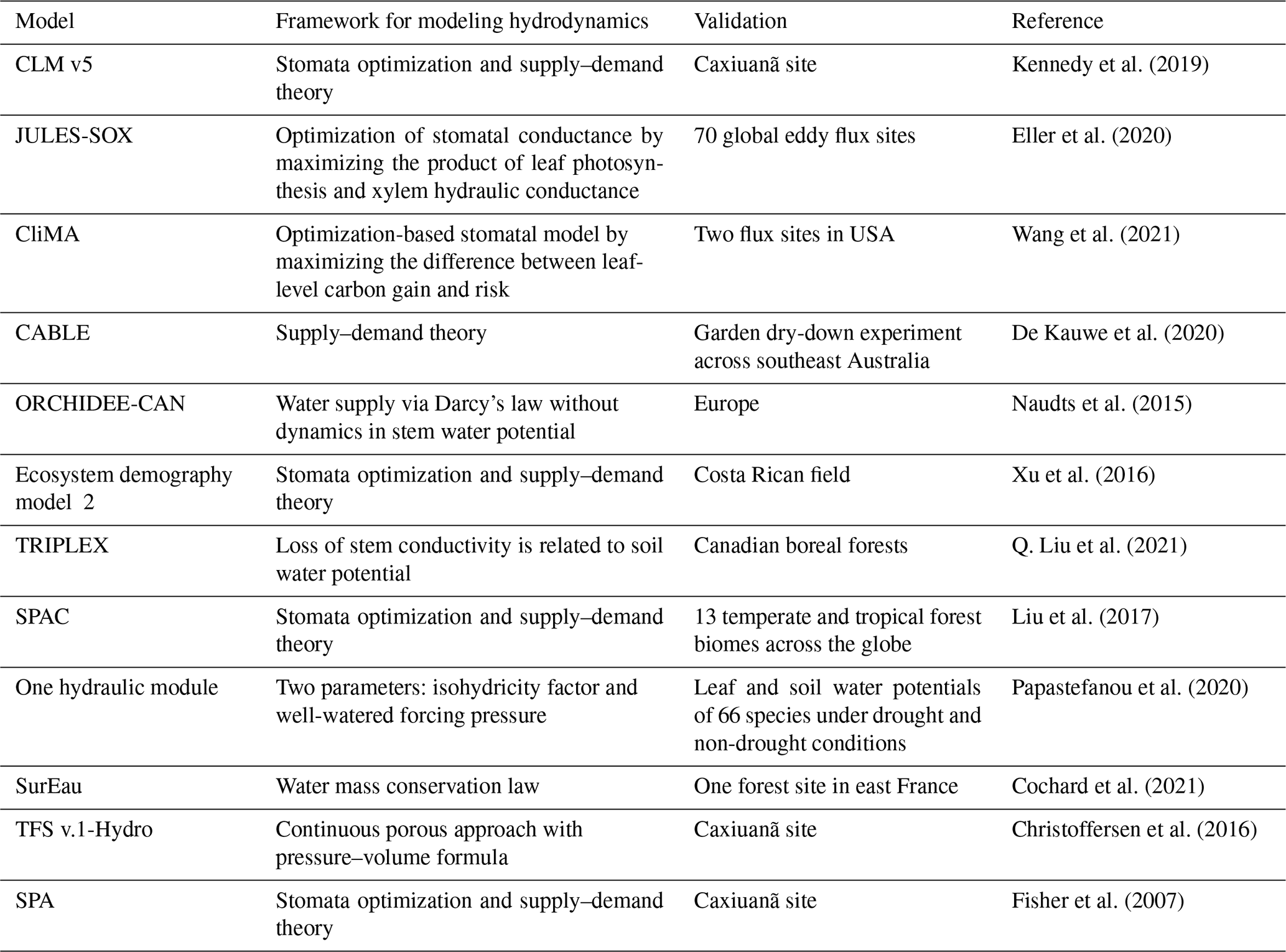
Table A2Parameters used in the new hydraulic architecture model. These parameters are selected from the range recorded by literature that we have analyzed.
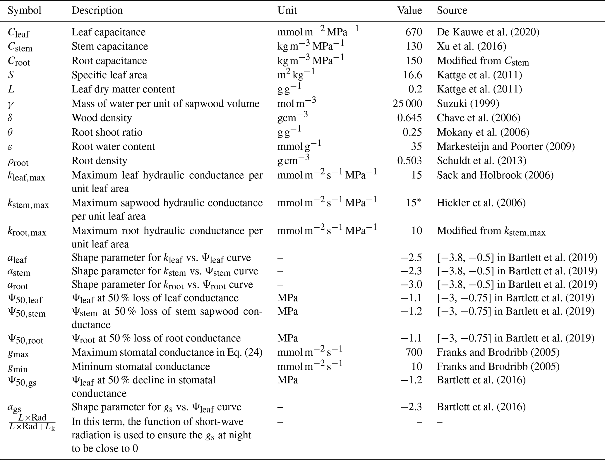
∗ In Hickler et al. (2006), the maximum sapwood conductivity of 50 × 10−4 can be converted to ∼ 15 if we assume sapwood area/leaf area of 0.0016 (value falls in Gotsch et al., 2010), and tree height of 30 m.
The ORCHIDEE-CAN-NHA model (r7236) code used in this study is deposited at https://forge.ipsl.jussieu.fr/orchidee/browser/branches/publications/ORCHIDEE_CAN_NHA (last access: 17 June 2021) and archived at https://doi.org/10.14768/8C2D06FB-0020-4BC5-A831-C876F5FBBFE9 (Yao, 2021a). The detailed code used to reproduce the analysis and figures is publicly available at https://doi.org/10.5281/zenodo.5721245 (Yao, 2021b).
The supplement related to this article is available online at: https://doi.org/10.5194/gmd-15-7809-2022-supplement.
YY, EJ, PC and NV designed the study. YY and EJ developed the code. YY conducted the analysis. YY wrote the manuscript. All authors provided comments and contributed to the final version of the paper.
The contact author has declared that none of the authors has any competing interests.
Publisher's note: Copernicus Publications remains neutral with regard to jurisdictional claims in published maps and institutional affiliations.
This research has been supported by the Centre National de la Recherche Scientifique, Institut écologie et environnement (grant no. 16-CONV-0003 and “Make Our Planet Great Again Scholarship” grant).
This paper was edited by Jinkyu Hong and reviewed by two anonymous referees.
Adams, H. D., Williams, A. P., Xu, C., Rauscher, S. A., Jiang, X., and McDowell, N. G.: Empirical and process-based approaches to climate-induced forest mortality models, Front. Plant Sci., 4, 438, https://doi.org/10.3389/fpls.2013.00438, 2013.
Adams, H. D., Zeppel, M. J., Anderegg, W. R., Hartmann, H., Landhäusser, S. M., Tissue, D. T., Huxman, T. E., Hudson, P. J., Franz, T. E., and Allen, C. D.: A multi-species synthesis of physiological mechanisms in drought-induced tree mortality, Nature Ecology & Evolution, 1, 1285–1291, 2017.
Aleixo, I., Norris, D., Hemerik, L., Barbosa, A., Prata, E., Costa, F., and Poorter, L.: Amazonian rainforest tree mortality driven by climate and functional traits, Nat. Clim. Change, 9, 384–388, 2019.
Allen, C. D., Macalady, A. K., Chenchouni, H., Bachelet, D., McDowell, N., Vennetier, M., Kitzberger, T., Rigling, A., Breshears, D. D., and Hogg, E. T.: A global overview of drought and heat-induced tree mortality reveals emerging climate change risks for forests, Forest Ecol. Manag., 259, 660–684, 2010.
Allen, C. D., Breshears, D. D., and McDowell, N. G.: On underestimation of global vulnerability to tree mortality and forest die-off from hotter drought in the Anthropocene, Ecosphere, 6, 1–55, 2015.
Anderegg, W. R.: Spatial and temporal variation in plant hydraulic traits and their relevance for climate change impacts on vegetation, New Phytol., 205, 1008–1014, 2015.
Anderegg, W. R., Flint, A., Huang, C.-y., Flint, L., Berry, J. A., Davis, F. W., Sperry, J. S., and Field, C. B.: Tree mortality predicted from drought-induced vascular damage, Nat. Geosci., 8, 367–371, 2015.
Anderegg, W. R., Konings, A. G., Trugman, A. T., Yu, K., Bowling, D. R., Gabbitas, R., Karp, D. S., Pacala, S., Sperry, J. S., and Sulman, B. N.: Hydraulic diversity of forests regulates ecosystem resilience during drought, Nature, 561, 538–541, 2018.
Bartlett, M. K., Klein, T., Jansen, S., Choat, B., and Sack, L.: The correlations and sequence of plant stomatal, hydraulic, and wilting responses to drought, P. Natl. Acad. Sci. USA, 113, 13098–13103, 2016.
Bartlett, M. K., Detto, M., and Pacala, S. W.: Predicting shifts in the functional composition of tropical forests under increased drought and CO2 from trade-offs among plant hydraulic traits, Ecol. Lett., 22, 67–77, 2019.
Bennett, A., McDowell, N., Allen, C., and Anderson-Teixeira, K. J.: Larger trees suffer most during drought in forests worldwide, Nature Plants, 1, 15139, https://doi.org/10.1038/nplants.2015.139, 2015.
Bittencourt, P. R., Oliveira, R. S., da Costa, A. C., Giles, A. L., Coughlin, I., Costa, P. B., Bartholomew, D. C., Ferreira, L. V., Vasconcelos, S. S., and Barros, F. V.: Amazonia trees have limited capacity to acclimate plant hydraulic properties in response to long-term drought, Glob. Change Biol., 26, 3569–3584, 2020.
Blackman, C. J., Pfautsch, S., Choat, B., Delzon, S., Gleason, S. M., and Duursma, R. A.: Toward an index of desiccation time to tree mortality under drought, Plant Cell Environ., 39, 2342–2345, 2016.
Blackman, C. J., Li, X., Choat, B., Rymer, P. D., De Kauwe, M. G., Duursma, R. A., Tissue, D. T., and Medlyn, B. E.: Desiccation time during drought is highly predictable across species of Eucalyptus from contrasting climates, New Phytol., 224, 632–643, 2019.
Bonan, G. B., Williams, M., Fisher, R. A., and Oleson, K. W.: Modeling stomatal conductance in the earth system: linking leaf water-use efficiency and water transport along the soil–plant–atmosphere continuum, Geosci. Model Dev., 7, 2193–2222, https://doi.org/10.5194/gmd-7-2193-2014, 2014.
Brienen, R. J., Phillips, O. L., Feldpausch, T. R., Gloor, E., Baker, T. R., Lloyd, J., Lopez-Gonzalez, G., Monteagudo-Mendoza, A., Malhi, Y., and Lewis, S. L.: Long-term decline of the Amazon carbon sink, Nature, 519, 344–348, 2015.
Brodribb, T. J., and Cochard, H.: Hydraulic failure defines the recovery and point of death in water-stressed conifers, Plant Physiol., 149, 575–584, 2009.
Brodribb, T. J., Powers, J., Cochard, H., and Choat, B.: Hanging by a thread? Forests and drought, Science, 368, 261–266, 2020.
Carswell, F., Costa, A., Palheta, M., Malhi, Y., Meir, P., de Pr Costa, J., Ruivo, M. d. L., do Sm Leal, L., Costa, J., and Clement, R.: Seasonality in CO2 and H2O flux at an eastern Amazonian rain forest, J. Geophys. Res.-Atmos., 107, LBA 43-41–LBA 43-16, 2002.
Chave, J., Muller-Landau, H. C., Baker, T. R., Easdale, T. A., Steege, H. T., and Webb, C. O.: Regional and phylogenetic variation of wood density across 2456 neotropical tree species, Ecol. Appl., 16, 2356–2367, 2006.
Choat, B.: Predicting thresholds of drought-induced mortality in woody plant species, Tree Physiol., 33, 669–671, 2013.
Choat, B., Brodribb, T. J., Brodersen, C. R., Duursma, R. A., López, R., and Medlyn, B. E.: Triggers of tree mortality under drought, Nature, 558, 531–539, 2018.
Christoffersen, B. O., Gloor, M., Fauset, S., Fyllas, N. M., Galbraith, D. R., Baker, T. R., Kruijt, B., Rowland, L., Fisher, R. A., Binks, O. J., Sevanto, S., Xu, C., Jansen, S., Choat, B., Mencuccini, M., McDowell, N. G., and Meir, P.: Linking hydraulic traits to tropical forest function in a size-structured and trait-driven model (TFS v.1-Hydro), Geosci. Model Dev., 9, 4227–4255, https://doi.org/10.5194/gmd-9-4227-2016, 2016.
Cochard, H. and Delzon, S.: Hydraulic failure and repair are not routine in trees, Ann. For. Sci., 70, 659–661, 2013.
Cochard, H., Pimont, F., Ruffault, J., and Martin-StPaul, N.: SurEau: a mechanistic model of plant water relations under extreme drought, Ann. For. Sci., 78, 1–23, 2021.
da Costa, A. C. L., Galbraith, D., Almeida, S., Portela, B. T. T., da Costa, M., Junior, J. d. A. S., Braga, A. P., de Gonçalves, P. H., de Oliveira, A. A., and Fisher, R.: Effect of 7 yr of experimental drought on vegetation dynamics and biomass storage of an eastern Amazonian rainforest, New Phytol., 187, 579–591, 2010.
De Kauwe, M. G., Medlyn, B. E., Ukkola, A. M., Mu, M., Sabot, M. E., Pitman, A. J., Meir, P., Cernusak, L., Rifai, S. W., and Choat, B.: Identifying areas at risk of drought-induced tree mortality across South-Eastern Australia, Glob. Change Biol., 26, 5716–5733, 2020.
Delbart, N., Ciais, P., Chave, J., Viovy, N., Malhi, Y., and Le Toan, T.: Mortality as a key driver of the spatial distribution of aboveground biomass in Amazonian forest: results from a dynamic vegetation model, Biogeosciences, 7, 3027–3039, https://doi.org/10.5194/bg-7-3027-2010, 2010.
Dewar, R., Mauranen, A., Mäkelä, A., Hölttä, T., Medlyn, B., and Vesala, T.: New insights into the covariation of stomatal, mesophyll and hydraulic conductances from optimization models incorporating nonstomatal limitations to photosynthesis, New Phytol., 217, 571–585, 2018.
Duffy, P. B., Brando, P., Asner, G. P., and Field, C. B.: Projections of future meteorological drought and wet periods in the Amazon, P. Natl. Acad. Sci. USA, 112, 13172–13177, 2015.
Eller, C. B., Rowland, L., Oliveira, R. S., Bittencourt, P. R., Barros, F. V., da Costa, A. C., Meir, P., Friend, A. D., Mencuccini, M., and Sitch, S.: Modelling tropical forest responses to drought and El Niño with a stomatal optimization model based on xylem hydraulics, Philos. T. R. Soc. B, 373, 20170315, https://doi.org/10.1098/rstb.2017.0315, 2018.
Eller, C. B., Rowland, L., Mencuccini, M., Rosas, T., Williams, K., Harper, A., Medlyn, B. E., Wagner, Y., Klein, T., and Teodoro, G. S.: Stomatal optimization based on xylem hydraulics (SOX) improves land surface model simulation of vegetation responses to climate, New Phytol., 226, 1622–1637, 2020.
Esquivel-Muelbert, A., Galbraith, D., Dexter, K. G., Baker, T. R., Lewis, S. L., Meir, P., Rowland, L., da Costa, A. C. L., Nepstad, D., and Phillips, O. L.: Biogeographic distributions of neotropical trees reflect their directly measured drought tolerances, Sci. Rep.-UK, 7, 1–11, 2017.
Fajardo, A.: Insights into intraspecific wood density variation and its relationship to growth, height and elevation in a treeline species, Plant Biol., 20, 456–464, 2018.
Fan, Z. X., Zhang, S. B., Hao, G. Y., Ferry Slik, J., and Cao, K. F.: Hydraulic conductivity traits predict growth rates and adult stature of 40 Asian tropical tree species better than wood density, J. Ecol., 100, 732–741, 2012.
Fisher, R., Williams, M., Da Costa, A. L., Malhi, Y., Da Costa, R., Almeida, S., and Meir, P.: The response of an Eastern Amazonian rain forest to drought stress: results and modelling analyses from a throughfall exclusion experiment, Glob. Change Biol., 13, 2361–2378, 2007.
Fisher, R. A., Williams, M., Do Vale, R. L., Da Costa, A. L., and Meir, P.: Evidence from Amazonian forests is consistent with isohydric control of leaf water potential, Plant Cell Environ., 29, 151–165, 2006.
Franklin, J. F., Shugart, H. H., and Harmon, M. E.: Tree death as an ecological process, BioScience, 37, 550–556, 1987.
Franks, P., and Brodribb, T. J.: Stomatal control and water transport in the xylem. In: Holbrook NM, Zwieniecki MA, eds, Vascular transport in plants, New York, NY, USA: Academic Press, 69–89, https://doi.org/10.1016/B978-012088457-5/50006-X, 2005.
Gleason, S. M., Blackman, C. J., Cook, A. M., Laws, C. A., and Westoby, M.: Whole-plant capacitance, embolism resistance and slow transpiration rates all contribute to longer desiccation times in woody angiosperms from arid and wet habitats, Tree Physiol., 34, 275–284, 2014.
Gotsch, S. G., Geiger, E. L., Franco, A. C., Goldstein, G., Meinzer, F. C., and Hoffmann, W. A.: Allocation to leaf area and sapwood area affects water relations of co-occurring savanna and forest trees, Oecologia, 163, 291–301, 2010.
Grote, R., Gessler, A., Hommel, R., Poschenrieder, W., and Priesack, E.: Importance of tree height and social position for drought-related stress on tree growth and mortality, Trees, 30, 1467–1482, 2016.
Gustafson, E. J. and Sturtevant, B. R.: Modeling forest mortality caused by drought stress: implications for climate change, Ecosystems, 16, 60–74, 2013.
Hammond, W. M., Yu, K., Wilson, L. A., Will, R. E., Anderegg, W. R., and Adams, H. D.: Dead or dying? Quantifying the point of no return from hydraulic failure in drought-induced tree mortality, New Phytol., 223, 1834–1843, 2019.
Hartmann, H.: Carbon starvation during drought-induced tree mortality – are we chasing a myth?, J. Plant Hydraul., 2, e005, https://doi.org/10.20870/jph.2015.e005, 2015.
Hendrik, D. and Maxime, C.: Assessing drought-driven mortality trees with physiological process-based models, Agr. Forest Meteorol., 232, 279–290, 2017.
Hickler, T., Prentice, I. C., Smith, B., Sykes, M. T., and Zaehle, S.: Implementing plant hydraulic architecture within the LPJ Dynamic Global Vegetation Model, Global Ecol. Biogeogr., 15, 567–577, 2006.
Joetzjer, E., Maignan, F., Chave, J., Goll, D., Poulter, B., Barichivich, J., Maréchaux, I., Luyssaert, S., Guimberteau, M., Naudts, K., Bonal, D., and Ciais, P.: Effect of tree demography and flexible root water uptake for modeling the carbon and water cycles of Amazonia, Ecol. Modell., 469, 109969, https://doi.org/10.1016/j.ecolmodel.2022.109969, 2022.
Kattge, J., Diaz, S., Lavorel, S., Prentice, I. C., Leadley, P., Bönisch, G., Garnier, E., Westoby, M., Reich, P. B., and Wright, I. J.: TRY–a global database of plant traits, Glob. Change Biol., 17, 2905–2935, 2011.
Kattge, J., Bönisch, G., Díaz, S., et al.: TRY plant trait database-enhanced coverage and open access, Glob. Change Biol., 26, 119–188, 2020.
Kennedy, D., Swenson, S., Oleson, K. W., Lawrence, D. M., Fisher, R., Lola da Costa, A. C., and Gentine, P.: Implementing plant hydraulics in the community land model, version 5, J. Adv. Model. Earth Sy., 11, 485–513, 2019.
Klos, R. J., Wang, G. G., Bauerle, W. L., and Rieck, J. R.: Drought impact on forest growth and mortality in the southeast USA: an analysis using Forest Health and Monitoring data, Ecol. Appl., 19, 699–708, 2009.
Kraft, N. J., Metz, M. R., Condit, R. S., and Chave, J.: The relationship between wood density and mortality in a global tropical forest data set, New Phytol., 188, 1124–1136, 2010.
Lewis, S. L., Brando, P. M., Phillips, O. L., van der Heijden, G. M., and Nepstad, D.: The 2010 amazon drought, Science, 331, 554–554, 2011.
Lin, Y. S., Medlyn, B. E., Duursma, R. A., Prentice, I. C., Wang, H., Baig, S., Eamus, D., De Dios, V. R., Mitchell, P., and Ellsworth, D. S.: Optimal stomatal behaviour around the world, Nat. Clim. Change, 5, 459–464, 2015.
Liu, Q., Peng, C., Schneider, R., Cyr, D., Liu, Z., Zhou, X., and Kneeshaw, D.: TRIPLEX-Mortality model for simulating drought-induced tree mortality in boreal forests: Model development and evaluation, Ecol. Model., 455, 109652, https://doi.org/10.1016/j.ecolmodel.2021.109652, 2021.
Liu, Y., Parolari, A. J., Kumar, M., Huang, C.-W., Katul, G. G., and Porporato, A.: Increasing atmospheric humidity and CO2 concentration alleviate forest mortality risk, P. Natl. Acad. Sci. USA, 114, 9918–9923, 2017.
Liu, Y., Holtzman, N. M., and Konings, A. G.: Global ecosystem-scale plant hydraulic traits retrieved using model–data fusion, Hydrol. Earth Syst. Sci., 25, 2399–2417, https://doi.org/10.5194/hess-25-2399-2021, 2021.
Maréchaux, I., Bartlett, M. K., Sack, L., Baraloto, C., Engel, J., Joetzjer, E., and Chave, J.: Drought tolerance as predicted by leaf water potential at turgor loss point varies strongly across species within an Amazonian forest, Funct. Ecol., 29, 1268–1277, 2015.
Maréchaux, I., Saint-André, L., Bartlett, M. K., Sack, L., and Chave, J.: Leaf drought tolerance cannot be inferred from classic leaf traits in a tropical rainforest, J. Ecol., 108, 1030–1045, 2020.
Maréchaux, I., Langerwisch, F., Huth, A., Bugmann, H., Morin, X., Reyer, C. P., Seidl, R., Collalti, A., Dantas de Paula, M., and Fischer, R.: Tackling unresolved questions in forest ecology: The past and future role of simulation models, Ecol. Evol., 11, 3746–3770, 2021.
Markesteijn, L. and Poorter, L.: Seedling root morphology and biomass allocation of 62 tropical tree species in relation to drought-and shade-tolerance, J. Ecol., 97, 311–325, 2009.
Martinez-Vilalta, J., Anderegg, W. R., Sapes, G., and Sala, A.: Greater focus on water pools may improve our ability to understand and anticipate drought-induced mortality in plants, New Phytol., 223, 22–32, 2019.
McDowell, N., Pockman, W. T., Allen, C. D., Breshears, D. D., Cobb, N., Kolb, T., Plaut, J., Sperry, J., West, A., and Williams, D. G.: Mechanisms of plant survival and mortality during drought: why do some plants survive while others succumb to drought?, New Phytol., 178, 719–739, 2008.
McDowell, N., Allen, C. D., Anderson-Teixeira, K., Brando, P., Brienen, R., Chambers, J., Christoffersen, B., Davies, S., Doughty, C., and Duque, A.: Drivers and mechanisms of tree mortality in moist tropical forests, New Phytol., 219, 851–869, 2018.
McDowell, N. G., Beerling, D. J., Breshears, D. D., Fisher, R. A., Raffa, K. F., and Stitt, M.: The interdependence of mechanisms underlying climate-driven vegetation mortality, Trends Ecol. Evol., 26, 523–532, 2011.
Meinzer, F. C., Campanello, P. I., Domec, J.-C., Gatti, M. G., Goldstein, G., Villalobos-Vega, R., and Woodruff, D. R.: Constraints on physiological function associated with branch architecture and wood density in tropical forest trees, Tree Physiol., 28, 1609–1617, 2008.
Meir, P., Mencuccini, M., and Dewar, R. C.: Drought-related tree mortality: addressing the gaps in understanding and prediction, New Phytol., 207, 28–33, 2015.
Meir, P., Mencuccini, M., Binks, O., da Costa, A. L., Ferreira, L., and Rowland, L.: Short-term effects of drought on tropical forest do not fully predict impacts of repeated or long-term drought: gas exchange versus growth, Philos. T. R. Soc. B, 373, 20170311, https://doi.org/10.1098/rstb.2017.0311, 2018.
Mokany, K., Raison, R. J., and Prokushkin, A. S.: Critical analysis of root: shoot ratios in terrestrial biomes, Glob. Change Biol., 12, 84–96, 2006.
Naudts, K., Ryder, J., McGrath, M. J., Otto, J., Chen, Y., Valade, A., Bellasen, V., Berhongaray, G., Bönisch, G., Campioli, M., Ghattas, J., De Groote, T., Haverd, V., Kattge, J., MacBean, N., Maignan, F., Merilä, P., Penuelas, J., Peylin, P., Pinty, B., Pretzsch, H., Schulze, E. D., Solyga, D., Vuichard, N., Yan, Y., and Luyssaert, S.: A vertically discretised canopy description for ORCHIDEE (SVN r2290) and the modifications to the energy, water and carbon fluxes, Geosci. Model Dev., 8, 2035–2065, https://doi.org/10.5194/gmd-8-2035-2015, 2015.
Nepstad, D. C., Tohver, I. M., Ray, D., Moutinho, P., and Cardinot, G.: Mortality of large trees and lianas following experimental drought in an Amazon forest, Ecology, 88, 2259–2269, 2007.
Nobre, C. A. and Borma, L. D. S.: `Tipping points' for the Amazon forest, Curr. Opin. Env. Sust., 1, 28–36, 2009.
Nychka D, F. R., Paige J, Sain S, Gerber F., and Iverson M.: Fields: Tools for Spatial Data, University Corporation for Atmospheric Research, Boulder, CO, USA, https://doi.org/10.5065/D6W957CT, R package version 10.3, 2020.
Pammenter, N. W. and Van der Willigen, C.: A mathematical and statistical analysis of the curves illustrating vulnerability of xylem to cavitation, Tree Physiol., 18, 589–593, 1998.
Papastefanou, P., Zang, C. S., Pugh, T. A., Liu, D., Grams, T. E., Hickler, T., and Rammig, A.: A dynamic model for strategies and dynamics of plant water-potential regulation under drought conditions, Front. Plant Sci., 11, 373, https://doi.org/10.3389/fpls.2020.00373, 2020.
Phillips, O. L., Aragão, L. E., Lewis, S. L., Fisher, J. B., Lloyd, J., López-González, G., Malhi, Y., Monteagudo, A., Peacock, J., and Quesada, C. A.: Drought sensitivity of the Amazon rainforest, Science, 323, 1344–1347, 2009.
Pierce, D.: Interface to Unidata netCDF (Version 4 or Earlier) Format Data, https://cran.r-project.org/web/packages/ncdf4/ (last access: 1 February 2019), 2019.
Powell, T. L., Galbraith, D. R., Christoffersen, B. O., Harper, A., Imbuzeiro, H. M., Rowland, L., Almeida, S., Brando, P. M., da Costa, A. C. L., and Costa, M. H.: Confronting model predictions of carbon fluxes with measurements of Amazon forests subjected to experimental drought, New Phytol., 200, 350–365, 2013.
Powell, T. L., Koven, C. D., Johnson, D. J., Faybishenko, B., Fisher, R. A., Knox, R. G., McDowell, N. G., Condit, R., Hubbell, S. P., and Wright, S. J.: Variation in hydroclimate sustains tropical forest biomass and promotes functional diversity, New Phytol., 219, 932–946, 2018.
R Development Core Team: R: A language and environment for statistical computing, R Foundation for Statistical Computing, Vienna, Austria, http://www.R-project.org/ (last access: 1 February 2019), 2019.
Rao, K., Anderegg, W. R., Sala, A., Martínez-Vilalta, J., and Konings, A. G.: Satellite-based vegetation optical depth as an indicator of drought-driven tree mortality, Remote Sens. Environ., 227, 125–136, 2019.
Rowland, L., da Costa, A. C. L., Galbraith, D. R., Oliveira, R., Binks, O. J., Oliveira, A., Pullen, A., Doughty, C., Metcalfe, D., and Vasconcelos, S.: Death from drought in tropical forests is triggered by hydraulics not carbon starvation, Nature, 528, 119–122, 2015.
Rozendaal, D. M., Phillips, O. L., Lewis, S. L., Affum-Baffoe, K., Alvarez-Davila, E., Andrade, A., Aragão, L. E., Araujo-Murakami, A., Baker, T. R., and Bánki, O.: Competition influences tree growth, but not mortality, across environmental gradients in Amazonia and tropical Africa, Ecology, 101, e03052, https://doi.org/10.1002/ecy.3052, 2020.
Sabot, M. E., De Kauwe, M. G., Pitman, A. J., Medlyn, B. E., Verhoef, A., Ukkola, A. M., and Abramowitz, G.: Plant profit maximization improves predictions of European forest responses to drought, New Phytol., 226, 1638–1655, 2020.
Sack, L. and Holbrook, N. M.: Leaf hydraulics, Annu. Rev. Plant Biol., 57, 361–381, 2006.
Sapes, G., Roskilly, B., Dobrowski, S., Maneta, M., Anderegg, W. R., Martinez-Vilalta, J., and Sala, A.: Plant water content integrates hydraulics and carbon depletion to predict drought-induced seedling mortality, Tree Physiol., 39, 1300–1312, 2019.
Schuldt, B., Leuschner, C., Brock, N., and Horna, V.: Changes in wood density, wood anatomy and hydraulic properties of the xylem along the root-to-shoot flow path in tropical rainforest trees, Tree Physiol., 33, 161–174, 2013.
Signori-Müller, C., Oliveira, R. S., de Vasconcellos Barros, F., Tavares, J. V., Gilpin, M., Diniz, F. C., Zevallos, M. J. M., Yupayccana, C. A. S., Acosta, M., and Bacca, J.: Non-structural carbohydrates mediate seasonal water stress across Amazon forests, Nat. Commun., 12, 1–9, 2021.
Sperry, J. S., Wang, Y., Wolfe, B. T., Mackay, D. S., Anderegg, W. R., McDowell, N. G., and Pockman, W. T.: Pragmatic hydraulic theory predicts stomatal responses to climatic water deficits, New Phytol., 212, 577–589, 2016.
Sperry, J. S., Venturas, M. D., Anderegg, W. R., Mencuccini, M., Mackay, D. S., Wang, Y., and Love, D. M.: Predicting stomatal responses to the environment from the optimization of photosynthetic gain and hydraulic cost, Plant Cell Environ., 40, 816–830, 2017.
Stovall, A. E., Shugart, H., and Yang, X.: Tree height explains mortality risk during an intense drought, Nat. Commun., 10, 1–6, 2019.
Suzuki, E.: Diversity in specific gravity and water content of wood among Bornean tropical rainforest trees, Ecol. Res., 14, 211–224, 1999.
Trugman, A. T., Anderegg, L. D., Anderegg, W. R., Das, A. J., and Stephenson, N. L.: Why is tree drought mortality so hard to predict?, Trends Ecol. Evol., 36, 520–532, https://doi.org/10.1016/j.tree.2021.02.001, 2021.
Urli, M., Porté, A. J., Cochard, H., Guengant, Y., Burlett, R., and Delzon, S.: Xylem embolism threshold for catastrophic hydraulic failure in angiosperm trees, Tree Physiol., 33, 672–683, 2013.
Van Genuchten, M. T.: A closed-form equation for predicting the hydraulic conductivity of unsaturated soils, Soil Sci. Soc. Am. J., 44, 892–898, 1980.
Wang, W., Peng, C., Kneeshaw, D. D., Larocque, G. R., and Luo, Z.: Drought-induced tree mortality: ecological consequences, causes, and modeling, Environ. Rev., 20, 109–121, 2012.
Wang, Y., Köhler, P., He, L., Doughty, R., Braghiere, R. K., Wood, J. D., and Frankenberg, C.: Testing stomatal models at the stand level in deciduous angiosperm and evergreen gymnosperm forests using CliMA Land (v0.1), Geosci. Model Dev., 14, 6741–6763, https://doi.org/10.5194/gmd-14-6741-2021, 2021.
Xu, X., Medvigy, D., Powers, J. S., Becknell, J. M., and Guan, K.: Diversity in plant hydraulic traits explains seasonal and inter-annual variations of vegetation dynamics in seasonally dry tropical forests, New Phytol., 212, 80–95, 2016.
Yang, Y., Saatchi, S. S., Xu, L., Yu, Y., Choi, S., Phillips, N., Kennedy, R., Keller, M., Knyazikhin, Y., and Myneni, R. B.: Post-drought decline of the Amazon carbon sink, Nat. Commun., 9, 1–9, 2018.
Yao, Y.: ORCHIDEE-CAN-NHA model (r7236), IPSL Data Catalog [code], https://doi.org/10.14768/8C2D06FB-0020-4BC5-A831-C876F5FBBFE9, 2021a.
Yao, Y.: yitongyao56/ORCHIDEE-CAN-NHA: Data analysis code, Zenodo [code], https://doi.org/10.5281/zenodo.5721245, 2021b.
Yoshimura, K., Saiki, S.-T., Yazaki, K., Ogasa, M. Y., Shirai, M., Nakano, T., Yoshimura, J., and Ishida, A.: The dynamics of carbon stored in xylem sapwood to drought-induced hydraulic stress in mature trees, Sci. Rep.-UK, 6, 24513, https://doi.org/10.1038/srep24513, 2016.
Young, D. J., Stevens, J. T., Earles, J. M., Moore, J., Ellis, A., Jirka, A. L., and Latimer, A. M.: Long-term climate and competition explain forest mortality patterns under extreme drought, Ecol. Lett., 20, 78–86, 2017.
Zhu, D., Peng, S. S., Ciais, P., Viovy, N., Druel, A., Kageyama, M., Krinner, G., Peylin, P., Ottlé, C., Piao, S. L., Poulter, B., Schepaschenko, D., and Shvidenko, A.: Improving the dynamics of Northern Hemisphere high-latitude vegetation in the ORCHIDEE ecosystem model, Geosci. Model Dev., 8, 2263–2283, https://doi.org/10.5194/gmd-8-2263-2015, 2015.
Zhu, S.-D., Chen, Y.-J., Ye, Q., He, P.-C., Liu, H., Li, R.-H., Fu, P.-L., Jiang, G.-F., and Cao, K.-F.: Leaf turgor loss point is correlated with drought tolerance and leaf carbon economics traits, Tree Physiol., 38, 658–663, 2018.