Impact of changes in climate and CO₂ on the carbon storage potential of vegetation under limited water availability using SEIB-DGVM version 3.02

Documenting year-to-year variations in carbon storage potential in terrestrial ecosystems is crucial for the determination of carbon dioxide (CO₂) emissions. However, the magnitude, pattern, and inner biomass partitioning of carbon storage potential and the effect of the changes in climate and CO₂ on inner carbon stocks remain poorly quantified. Herein, we use a spatially explicit individual-based dynamic global vegetation model to investigate the influences of the changes in climate and CO₂ on the enhanced carbon storage potential of vegetation. The modelling included a series of factorial simulations using the Climatic Research Unit (CRU) dataset from 1916 to 2015. The results show that CO₂ predominantly leads to a persistent and widespread increase in light-gathering vegetation biomass carbon stocks (LVBC) and water-gathering vegetation biomass carbon stocks (WVBC). Climate change appears to play a secondary role in carbon storage potential. Importantly, with the intensification of water stress, the magnitude of the light- and water-gathering responses in vegetation carbon stocks gradually decreases. Plants adjust carbon allocation to decrease the ratio between LVBC and WVBC for capturing more water. Changes in the pattern of vegetation carbon storage were linked to zonal limitations in water, which directly weaken and indirectly regulate the response of potential vegetation carbon stocks to a changing environment. Our findings differ from previous modelling evaluations of vegetation that ignored inner carbon dynamics and demonstrate that the long-term trend in increased vegetation biomass carbon stocks is driven by CO₂ fertilization and temperature effects that are controlled by water limitations.

1 Introduction

As a result of the changes in climate and atmospheric carbon dioxide (CO₂), the terrestrial ecosystem carbon cycle exhibits remarkable trends in interannual variations, which induce uncertainty in estimated carbon budgets (Cheng et al., 2017; Erb et al., 2018; Fan et al., 2019; Keenan et al., 2016). Recent studies assessing interannual fluctuations in terrestrial carbon sinks have shown that the land carbon cycle is the most uncertain component of the global carbon budget (Ahlstrom et al., 2015; Piao et al., 2020; Jung et al., 2017; Humphrey et al., 2018; Gentine et al., 2019; Humphrey et al., 2021). These uncertainties result from an incomplete understanding of vegetation biomass carbon production, allocation, storage, loss, and turnover time (Bloom et al., 2016). The extent and distribution of vegetation carbon storage is central to our understanding of how to maintain a balanced land carbon cycle. Changes in terrestrial vegetation carbon storage have a significant effect on atmospheric CO₂ concentrations and determine whether biomes become a source or sink of carbon (Erb et al., 2018; Humphrey et al., 2018; Terrer et al., 2021). Therefore, investigating the processes producing changes in carbon storage is key to improving the accuracy of estimated terrestrial carbon budgets and to tapping the greenhouse gas moderation potentials of vegetation (IPCC, 2007; Saugier et al., 2001).

The atmospheric CO₂ concentration is affected by the vegetation carbon stock, while the long-term trend of vegetation carbon storage capacity is also affected by the changes in climate and CO₂. Since the beginning of industrialization, there has been a noticeable enhancement in the plant capacity of storing and sequestering carbon, which is needed for stabilizing greenhouse gas concentrations and mitigating global warming (Chen et al., 2019; Pan et al., 2011; Piao et al., 2006; Le Noë et al., 2020; Magerl et al., 2019; Bayer et al., 2015; Harper et al., 2018). Due to the interaction between terrestrial vegetation and a changing environment, both photosynthesis and respiration of the vegetation also changed. To better absorb CO₂ and sunlight required for photosynthesis, vegetated zones are gradually covered by vegetation with higher plant height and wider leaf area (Erb et al., 2008). This change has coincided with a widespread change in other vegetation features, including a positive increase in annual gross primary productivity and a greening of the biosphere (Madani et al., 2020; Zhu et al., 2016). The spatiotemporal distribution and environmental drivers in total carbon storage potential have been well documented on the basis of model estimates and satellite-based assessments (Erb et al., 2007, 2018; Bazilevich et al., 1971; Saugier et al., 2001; Bartholome and Belward, 2005; Olson et al., 1983; Pan et al., 2013; Ajtay et al., 1979; Ruesch and Gibbs, 2008; Kaplan et al., 2011; Shevliakova et al., 2009; Prentice et al., 2011; West et al., 2010; Hurtt et al., 2011). In contrast, the variability in inner components of carbon storage potential has not been extensively studied. Without an accurate assessment of the dynamics of each fraction, attribution of carbon storage potential to environmental drivers is highly uncertain. Consequently, partitioning potential vegetation carbon storage and revealing its inner processes are essential to accurately comprehend the current state of carbon storage capacity and reveal the influence of various drivers on the long-term trend of carbon storage potential.

The change in carbon storages in vegetation inner components is not only affected by environmental factors but also controlled by the allocation scheme of assimilated carbon (Friedlingstein et al., 1999). Fractional dynamics of the carbon stock are widely used as a key indicator to investigate the responses of vegetation to environmental drivers, which also reflect the response strategies of vegetation in environments with different water limitations (Yang et al., 2010). In arid regions, vegetation utilizes a tolerance strategy to allocate biomass, storing more biomass carbon in roots to resist enhanced water stress (Chen et al., 2013). Conforming to the optimal partitioning hypothesis, plants store more carbon in shoots and leaves in environments where water is more available and shift more carbon to roots when water is more limited (Yang et al., 2010; McConnaughay and Coleman, 1999). Water availability controls both carbon allocation and storage and can potentially transform zones characterized by a positive response to changes in climate and CO₂ to zones exhibiting a negative response. For example, global warming positively stimulates plant productivity (Keenan et al., 2016), while Madani et al. (2020) found that productivity showed a negative response to temperature in tropical zones due to increasing water stress. With increased warming, water limitations are predicted to increasingly reduce the proportion of leaves' biomass and decrease plant photosynthesis (Ma et al., 2021). Water limitations have a strong regulating effect on the spatial pattern of change in vegetation carbon storage, demonstrating that the effects of the changes in climate and CO₂ on the dynamics of the plant organs are affected by the terrestrial water gradient. Thus, it is important to systematically investigate the distinct responses of carbon storage potential to changes in climate and CO₂ under differing conditions of water stress.

As documented above, many studies have investigated the total changes in zonal and global terrestrial storage of carbon, while few studies have examined trends in the component partitioning of vegetation carbon storage. Large gaps in our knowledge of the effects of various drivers on the partitioning of carbon stocks in vegetation biomass remain. Meanwhile, plants adjust their carbon allocation scheme to adapt to environmental change. With increased warming, an increase in the magnitude of water stress may dramatically change or even reverse the impact of these drivers on inner components of carbon storage (Ma et al., 2021). Evaluating the response pattern of carbon stocks to various drivers under conditions of limited water is elemental for clearly documenting the response mechanism of vegetation carbon storage potential.

Here, we use a spatially explicit, individual-based dynamic global vegetation model (SEIB-DGVM), along with the component partitioning method to (1) systematically determine the long-term variability in carbon storage potential and understand its response mechanisms and (2) estimate trends in partitioning of potential biomass carbon stocks of vegetation biomass. Throughout this study, the potential biomass carbon stock, biomass carbon stored in vegetation without anthropogenic disturbance, is recognized as an indicator of the potential of carbon storage by natural vegetation. Using a set of factorial simulations to isolate responses to environmental change, we analyse the contributions of multiple driving factors to the trends of two fractions of carbon stock at large scales individually. We then conceptualize the role of water availability through an aridity index (AI), in which hydrological zones are subdivided by their degree of aridity. By comparing the differences in the magnitude of response between the fractions of light- and water-gathering carbon stocks for varying degrees of water availability, we assess the effect of water limitations on the response pattern of potential carbon stocks to changes in climate and CO₂.

2 Model description, experimental design, observational data, and evaluation metrics

In this section, we provide a list of data sources (Sect. 2.1), an overview of the modelling concept (Sect. 2.2), the representation of biomass carbon stock partitioning in the SEIB-DGVM (Sect. 2.3), an overview of the experimental scheme used in the model simulations (Sect. 2.4), and an overview about data sources and pre-processing of the observation dataset for model evaluation (Sect. 2.5).

2.1 Forcing data

Long-term daily meteorological time series data are required to run model simulations, including precipitation, daily range of air temperature, mean daily air temperature, downward shortwave radiation at midday, downward longwave radiation at midday, wind velocity, and relative humidity. These data were obtained from the Climatic Research Unit (CRU) time series 4.00 gridded dataset (degree 0.5^∘) for the period 1901–2015 (Harris et al., 2020). Because the CRU dataset is a monthly based dataset, the monthly meteorological data were converted into daily climatic variables by supplementing daily climatic variability within each month using the National Centers for Environmental Prediction (NCEP) daily climate dataset. The NCEP data, displayed using the T62 Gaussian grid with 192 × 94 points, were interpolated into a 0.5^∘ grid (which corresponds to the CRU dataset) using a linear interpolation method. By combining the CRU data with the interpolated NCEP dataset, we were able to directly obtain most of the driving meteorological data (details in Sato et al., 2020). Neither the CRU nor NCEP datasets included downward shortwave and longwave radiation at midday. Thus, daily cloudiness values in the NCEP were used to calculate radiation values using empirical functions (Sato et al., 2007). These data were all aggregated to a daily timescale with 0.5^∘ resolution to run SEIB-DGVM.

Atmospheric CO₂ concentrations were collected from Sato et al. (2020), who provide reconstructed CO₂ concentrations between 1901 and 2015. The statistical reconstruction of global atmospheric CO₂ was used in this analysis. These reconstructions were based on present annual CO₂ concentrations recorded from the Mauna Loa monitoring station. These data assume atmospheric CO₂ concentration was 284 ppm in 1750 and statistically interpolate atmospheric CO₂ concentrations to fill the gap from 1750 to 2015.

The physical parameters of the soil used in the model include soil moisture at the saturation point, field capacity, matrix potential, wilting point, and albedo. These data were obtained from the Global Soil Wetness Project 2.

2.2 Overview of modelling concept in SEIB-DGVM

Model SEIB-DGVM version 3.02 (Sato et al., 2020) was employed in this study. This is a process-based dynamic global vegetation model driven by meteorological and soil data. It is an explicit and computationally efficient carbon cycle model designed to simulate transient effects of environmental change on terrestrial ecosystems and land–atmosphere interactions. It describes three groups of processes: land-based physical processes (e.g. hydrology, radiation, aridity), plant physiological processes (e.g. photosynthesis, respiration, litter), and plant dynamic processes (e.g. establishment, growth, mortality). Twelve plant functional types (PFTs) were classified. During the simulation, a sample plot was established at each grid cell, and then the growth, competition, and mortality of each of the individual PFTs within each plot were modelled by considering the specific conditions for that individual as it relates to other individuals that surround it (Sato et al., 2007).

SEIB-DGVM treats the relationships between soil, atmosphere, and terrestrial biomes in a consistent manner, including the fluxes of energy, water, and carbon. Based on specified climatic conditions and soil properties, SEIB-DGVM simulates the carbon cycle, energy balance, and hydrological processes. SEIB-DGVM utilizes three computational time steps. (1) During the growth phase, the metabolic procedures including photosynthesis, respiration, and carbon allocation are executed for each individual tree every simulation day. (2) The monthly process of tree growth including reproduction, trunk growth, and expansion of a cross-sectional area of the crown are executed. (3) On the last day of each year, the height of the lowest branch increases as a result of purging crown disks, or self-pruning of branches, at the bottom of the crown layer. The simulated unit of the model is a 30 m × 30 m spatially explicit “virtual forest”. A grass layer was placed under the woody layer and provides for a comprehensive, spatially explicit quantification of terrestrial carbon sinks and sources. The soil depth was set at 2 m and was divided into 20 layers, each with a thickness of 0.1 m. The photosynthetic rate of a single leaf was simulated following a Michaelis-type function (Ryan, 1991). Respiration was divided into two types: growth respiration and maintenance respiration. Growth respiration is defined as a construction cost for plant biosynthesis, which is quantified by the chemical composition of each organ (Poorter, 1994). Maintenance respiration of live plants occurs every day regardless of the phenological phase and is controlled by the temperature and nitrate content of each organ (Ryan, 1991). For a wide variety of plant organs, the maintenance respiration rate is linearly related to the nitrogen content of living tissue. The relative proportions of nitrogen in each organ for any PFT are linearly correlated. Nitrogen deposition is not included in SEIB-DGVM. Atmospheric CO₂ was envisioned to be absorbed by photosynthesis of woody PFTs and grass PFTs. This assimilated carbon flux was then allocated into all the plant organs (leaf, trunk, root, and stock) where maintenance respiration and growth respiration occur. The hydrology module treats precipitation, canopy interception, transpiration, evaporation, meltwater, and penetration.

2.3 Carbon stock of vegetation biomass partitioning

2.3.1 Parameterization of daily allocation

Flexible allocation schemes about resources and biomass are set up in the framework of the SEIB-DGVM biogeochemical model. Based on the updated observation data, the allocation schemes of boreal needle-leaved summer-green trees and tropical broad-leaved evergreen trees are improved in SEIB-DGVM V3.02. Allocation schemes of other PFTs are the same as the original version. Atmospheric CO₂ is assimilated by the photosynthesis of both woody and grass foliage and then is added into the non-structural carbon of the plant. This non-structural carbon of photosynthetic production is allocated to all the plant organs (foliage, trunk, root, and stock), supplying what is needed for the maintenance and growth of each organ. When the non-structural carbon is greater than 0 during the growth phase, the following dynamic carbon allocation is executed for each individual plant at the daily timescale, such that the following can be said.

1. When the fine root biomass (mass_root) of wood or grass does not satisfy minimum requirements for fulfilling functional balance (mass_leaf $/$ FR_ratio), the mass of non-structural carbon is allocated to the root biomass to supplement the deficit. Here, mass_leaf is the leaf biomass, and FR_ratio is the ratio of mass_leaf to mass_root satisfying the functional balance.

2. The stock biomass is supplemented until it is equal to leaf biomass. This scheme is active after the first 30 d of the growing phase.

3. Woody leaf biomass is constrained by three limitations of the maximum leaf biomass, which are calculated as follows:

   $$\begin{array}{ll}{\displaystyle }{\max }_{\mathrm{1}}& {\displaystyle }=\left({\mathrm{crown}}_{\mathrm{area}}+\mathit{\pi }{\mathrm{crown}}_{\mathrm{diameter}}{\mathrm{crown}}_{\mathrm{depth}}\right)\\ \text{(1)}& {\displaystyle }& {\displaystyle \frac{{\mathrm{LA}}_{\max }}{\mathrm{SLA}}}{\displaystyle }{\max }_{\mathrm{2}}& {\displaystyle }={\mathrm{ALM}}_{\mathrm{1}}\\ \text{(2)}& {\displaystyle }& {\displaystyle \frac{\begin{array}{c}\mathit{\pi }{\left({\mathrm{dbh}}_{\mathrm{heartwood}}/\mathrm{2}+{\mathrm{dbh}}_{\mathrm{sapwood}}/\mathrm{2}\right)}^{\mathrm{2}}\\ -\mathit{\pi }{\left({\mathrm{dbg}}_{\mathrm{heartwood}}/\mathrm{2}\right)}^{\mathrm{2}}\end{array}}{\mathrm{SLA}}}\text{(3)}& {\displaystyle }{\max }_{\mathrm{3}}& {\displaystyle }={\displaystyle \frac{{\mathrm{mass}}_{\mathrm{available}}}{{\mathrm{RG}}_{\mathrm{f}}}}\text{(4)}& {\displaystyle }{\mathrm{mass}}_{\mathrm{leaf}}& {\displaystyle }=\min ({\max }_{\mathrm{1}},{\max }_{\mathrm{2}},{\max }_{\mathrm{3}}),\end{array}$$

   where max₁, max₂, and max₃ are, respectively, maximum leaf biomass for a given crown surface area, cross-sectional area of sapwood, and non-structural carbon; the constant of specific leaf area (SLA) is the PFT-specific leaf area per unit biomass (m² g⁻¹); LA_max is the plant-functional-type-specific maximum leaf area per unit crown surface area excluding the bottom layer (m² m⁻²); ALM₁ represents the area of transport tissue per unit biomass and is a constant (dimensionless). If the mass_leaf is less than the minimum $({\max }_{\mathrm{1}},{\max }_{\mathrm{2}},{\max }_{\mathrm{3}}$), the mass of non-structural carbon is allocated into leaf biomass to supplement the deficit.

   When the leaf area index of grass equals the optimal leaf area index, it stops allocating non-structural carbon to grass leaf, which is calculated as

   $$\begin{array}{}\text{(5)}& \begin{array}{rl}& {\mathrm{lai}}_{\mathrm{opt}}=\\ & {\displaystyle \frac{\ln {\mathrm{par}}_{\mathrm{grass}}-\ln \left\{\frac{p_{\mathrm{sat}}}{\mathrm{lue}}\left[{\left(\mathrm{1}-\frac{\mathrm{cost}/\mathrm{SLA}}{\mathrm{0.09093}\times \mathrm{dlen}\times p_{\mathrm{sat}}}\right)}^{-\mathrm{2}}-\mathrm{1}\right]\right\}}{\mathrm{eK}}}\end{array},\end{array}$$

   where lai_opt is the optimal leaf area index (m² m⁻²), par_grass is the grass photosynthetically active radiation (µmol photon m⁻² s⁻¹), p_sat is the light-saturated photosynthetic rate (µCO₂ m⁻² s⁻¹), lue is the light use efficiency of photosynthesis (mol CO₂ mol photon⁻¹), cost is the cost of maintaining leaves per unit dry leaf mass (DM) per day (g DM g DM⁻¹ d⁻¹), dlen is day length (hour), and eK is light attenuation coefficient at midday.

4. When non-structural carbon is less than 10 g DM PFT⁻¹, or annual net primary production (NPP) is less than 10 g DM PFT⁻¹ in the previous year, the following daily simulation processes (5–6) will be skipped.

5. When total woody biomass is more than 10 kg DM, which defines the minimum tree size for reproduction, 10 % of non-structural carbon is used for every daily process of reproduction, including having flowers, pollen, nectar, fruits, and seeds. These organs are not explicitly modelled in SEIB-DGVM.

6. During the simulation of trunk growth, the remaining non-structural carbon is allocated to sapwood biomass. There is no direct allocation to heartwood, which is transformed slowly from sapwood biomass. For grass PFTs biomass, the densities of all organs comprising the biomass never decline below 0.1 g DM m⁻² even if the environment is deteriorated for grass survival. A more detailed description of SEIB-DGVM is given by Sato et al. (2007).

   To control plant phenology and the rate of photosynthesis as a function of the limitation in terrestrial water, the physiological status of the limitation of terrestrial water is calculated as

   $$\begin{array}{ll}\text{(6)}& {\displaystyle }& {\displaystyle }{p}_{\mathrm{sat}}={\mathrm{PMAXce}}_{\mathrm{tmp}}{\mathrm{ce}}_{{\mathrm{CO}}_{\mathrm{2}}}{\mathrm{ce}}_{\mathrm{water}}\text{(7)}& {\displaystyle }& {\displaystyle }{\mathrm{ce}}_{\mathrm{water}}=\sqrt{{\mathrm{stat}}_{\mathrm{water}}}{\displaystyle }& {\displaystyle }{\mathrm{stat}}_{\mathrm{water}}=\\ \text{(8)}& {\displaystyle }& {\displaystyle \frac{max\left({\mathrm{pool}}_{\mathrm{w}\left(\mathrm{1}\right)}/{\mathrm{Depth}}_{\left(\mathrm{1}\right)},{\mathrm{pool}}_{\mathrm{w}\left(\mathrm{2}\right)}/{\mathrm{Depth}}_{\left(\mathrm{2}\right)}\right)-W_{\mathrm{wilt}}}{W_{\mathrm{fi}}-W_{\mathrm{wilt}}}},\end{array}$$

   where p_sat is the single-leaf photosynthetic rate of tree PFTs and grass PFTs (µmol CO₂ m⁻² s⁻¹); PMAX is the potential maximum of photosynthetic rate (µmol mol⁻¹ CO₂ m⁻² s⁻¹); ce_tmp and ${\mathrm{ce}}_{{\mathrm{CO}}_{\mathrm{2}}}$ are the temperature and CO₂ concentration effect coefficient (dimensionless), separately; ce_water is the water effect coefficient (dimensionless); stat_water is the physiological status of the terrestrial water limitation, which ranges between 0.0–1.0 (dimensionless); pool_w(n) is the water content in soil layer n (mm); Depth_(n) is the depth of the soil layer n (mm); W_wilt is soil moisture at the wilting point (m m⁻¹); and W_fi is soil moisture at field capacity (m m⁻¹). When the temperature of all soil layers is less than 0 ^∘C, stat_water equals 0.

2.3.2 Carbon stock partitioning method

SEIB-DGVM allocates and stores the biomass carbon in four pools of woody PFT (foliage, trunk, root, and stock) and three pools of grass PFT (foliage, root, and stock). To investigate the fractional variability in carbon sequestration potential between the pools, we partitioned potential vegetation carbon stocks based on the physiological function of the plant (Fig. A1). The root–shoot ratio (R $/$ S) has been used to distinguish and investigate the ratio of belowground biomass (root biomass) and aboveground biomass (shoot biomass) (Zhang et al., 2016). In this study, we adjusted the method of calculating the R $/$ S ratio by distinguishing between the light-gathering vegetation biomass carbon stock (LVBC) and the water-gathering vegetation biomass carbon stock (WVBC). LVBC represents the biomass carbon invested by a plant that is used to gather sunlight, including biomass carbon from woody foliage, woody trunk, and grass foliage. WVBC represents biomass carbon used to gather water, including biomass carbon from woody fine roots and grass fine roots, excluding the stock pool. Stock biomass is used for foliation after the dormant phase and after fires and is a reserve resource in each individual tree. Fine root biomass is just a tiny fraction of the total biomass but has a very high turnover rate and determines the capacity of vegetation to absorb soil water. Thus,

$$\begin{array}{}\text{(9)}& {\displaystyle \frac{\mathrm{LVBC}}{\mathrm{WVBC}}}={\displaystyle \frac{{\mathrm{Tmass}}_{\mathrm{leaf}}+{\mathrm{Tmass}}_{\mathrm{trunk}}+{\mathrm{Gmass}}_{\mathrm{leaf}}}{{\mathrm{Tmass}}_{\mathrm{root}}+{\mathrm{Gmass}}_{\mathrm{root}}}}\times \mathrm{100}\mathit{\%},\end{array}$$

where LVBC is light-gathering vegetation biomass carbon stock (kg C m⁻²); WVBC is water-gathering vegetation biomass carbon stock (kg C m⁻²); Tmass_leaf is the leaf biomass carbon stock of woody vegetation (kg C m⁻²); and Tmass_trunk is the trunk biomass carbon stock of trees (kg C m⁻²), including both branch and structural roots. This biomass is simplistically attributed to light-gathering vegetation organs and is used primarily to support the plant. Gmass_leaf is the leaf biomass carbon stock of grass (kg C m⁻²), whereas Tmass_root and Gmass_root are functional root (fine roots) biomass carbon stocks of trees and grass, separately (kg C m⁻²), which absorb water and nutrition from soil.

2.4 Experimental design

2.4.1 Setup of model runs

SEIB-DGVM simulations begin with seeds of selected PFTs planted in bare ground. The establishment of PFT seeds is determined by the climatic conditions in each grid cell. We inputted the transient climate data from 1901 to 1915 to spin up the model in a repetitive loop. No obvious trend in climatic factors was observed during this period (Tei et al., 2017). A spin-up period of 1050 years was necessary to bring the terrestrial vegetation carbon cycle into a dynamic equilibrium. To reach quasi-equilibrium in the vegetation biomass, about 1000 years of simulation was required as a spin-up procedure.

2.4.2 Factorial simulation scheme

In order to further quantify the relative contributions of varying atmospheric CO₂ concentrations, precipitation, temperature, radiation, and other factors (wind velocity and relative humidity), we performed six factorial simulations. In simulation S1, atmospheric CO₂ concentration and all climate variables were varied. In simulation S2, only atmospheric CO₂ concentration was varied, and climate variables were held constant (climate variables of the transient period, 1901–1915 were repeatedly inputted). In simulation S3 (or S4 and S5), atmospheric CO₂ and precipitation (or temperature and radiation) were varied, and other climate variables were held constant. In simulation S6, atmospheric CO₂, wind velocity, and relative humidity were varied, and other climate variables were held constant. Finally, S2 was used to evaluate the effects of CO₂ fertilization on carbon stock variation. The differences in S2–S3, S2–S4, S2–S5, and S2–S6 were used to evaluate the response of carbon stock growth to precipitation, temperature, radiation, and other drivers, respectively.

Table 1 List of factorial simulations used in this study.

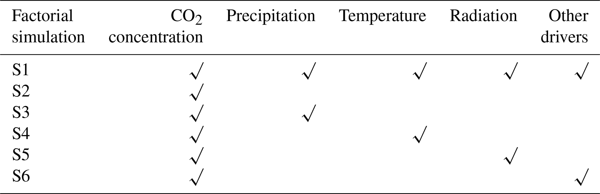
Note: in factorial simulation S1, historical atmospheric CO₂ concentration and historical climate fields from the CRU dataset were used. In simulation S2, only historical atmospheric CO₂ concentration was used, and climate variables of the transient period (1901–1915) were repeatedly input. In simulation S3 (or S4 or S5), only historical atmospheric CO₂ concentrations and precipitation (or temperature or radiation) were input, and climate variables of the transient period (1901–1915) were repeatedly input. In the last simulation, S6, only historical atmospheric CO₂ concentrations and other climate variables were input, including wind velocity and relative humidity.

2.4.3 Non-parametric test methods

Each driving factor (atmosphere CO₂, precipitation, temperature, and radiation) has a different influence on the carbon stock, so it is difficult to make a simple pre-assumption about the population distribution pattern for factorial simulations. We used the non-parametric Mann–Kendall and Sen slope estimator statistical tests (Gocic and Trajkovic, 2013) to assess the ability of SEIB-DGVM to simulate the response patterns of carbon storage potential to a change in climate and CO₂ concentrations. We regressed the simulated 100-year mean global average carbon stock time series to reveal the accumulative influences of the single variables based on the factorial simulations where only one or two drivers were varied. As shown in Figs. A2 and A3, detection trends of LVBC and WVBC for all driving factors performed statistically well (in agreement at the 95 % confidence intervals), indicating that this analytical method was suitable for trend attribution at the global scale.

2.4.4 Distinguishing hydrological regions

Locally available water strongly regulates and limits the response of carbon stocks to changes in climate and CO₂. We used aridity index (AI) to distinguish between the global hydrological regions for comparing the long-term trend in carbon stocks over different hydrological environments and for quantifying the influences of each hydrological environment on the variations in the trends. The AI was defined as

$$\begin{array}{}\text{(10)}& \mathrm{AI}={\displaystyle \frac{\stackrel{\mathrm{‾}}{P}}{\stackrel{\mathrm{‾}}{{\mathrm{ET}}_{\mathrm{p}}}}},\end{array}$$

where $\stackrel{\mathrm{‾}}{P}$ is the multiyear mean precipitation (mm yr⁻¹), and $\stackrel{\mathrm{‾}}{{\mathrm{ET}}_{\mathrm{p}}}$ is the multiyear mean potential evapotranspiration (mm yr⁻¹), which was calculated by the Penman–Monteith model (Monteith and Unsworth, 1990). As in a previous study (Chen et al., 2019), five hydrological regions were categorized based on AI value. Under the influences of climate change, the hydrological condition was changed in some grid cells (Fig. A4). For example, the grid cell classified as sub-humid zone in the period of 1916–1945 was redefined as semi-arid zone in the period of 1986–2015. In this study, grid cells with consistent hydrological condition between the period of 1916–1945 and the period of 1986–2015 were selected and classified (Fig. 1).

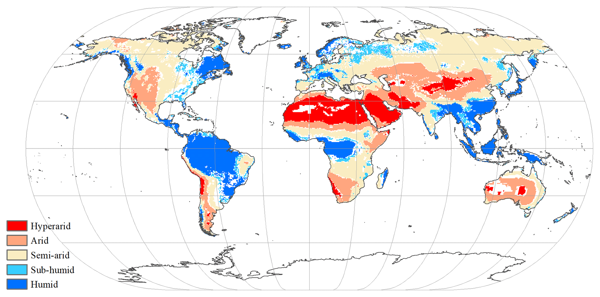
Figure 1 Global spatial patterns of water availability. Spatial variations in water availability were categorized based on the multiyear average aridity index (AI), defined as the ratio of the multiyear mean precipitation to the potential evapotranspiration. Categories include hyper-arid (AI ≤ 0.05), arid (0.05 < AI ≤ 0.2), semi-arid (0.2 < AI ≤ 0.5), sub-humid (0.5 < AI ≤ 0.65), and humid (AI > 0.65). The white grid cells were not assigned a hydrological category.

2.5 Observation dataset for model evaluation

A global time series of potential vegetation carbon was modelled by the SEIB-DGVM between 1916–2015. In terrestrial vegetation biomes, there is a high correlation between biomass carbon stock density and NPP per unit (Erb et al., 2016; Kindermann et al., 2008) (Fig. A1). Thus, we collected the NPP observation dataset and used NPP as a proxy for the carbon stock to assess model accuracy. Ecosystem Model–Data Intercomparison (EMDI) builds upon the accomplishments of the original worldwide synthesis of NPP measurements and associated model driver data prepared by the Global Primary Production Data Initiative. We obtained the monitoring station data from the EMDI working group and then compared their data with modelled multiyear average NPP in the period of 1916–1999 (Fig. 2).

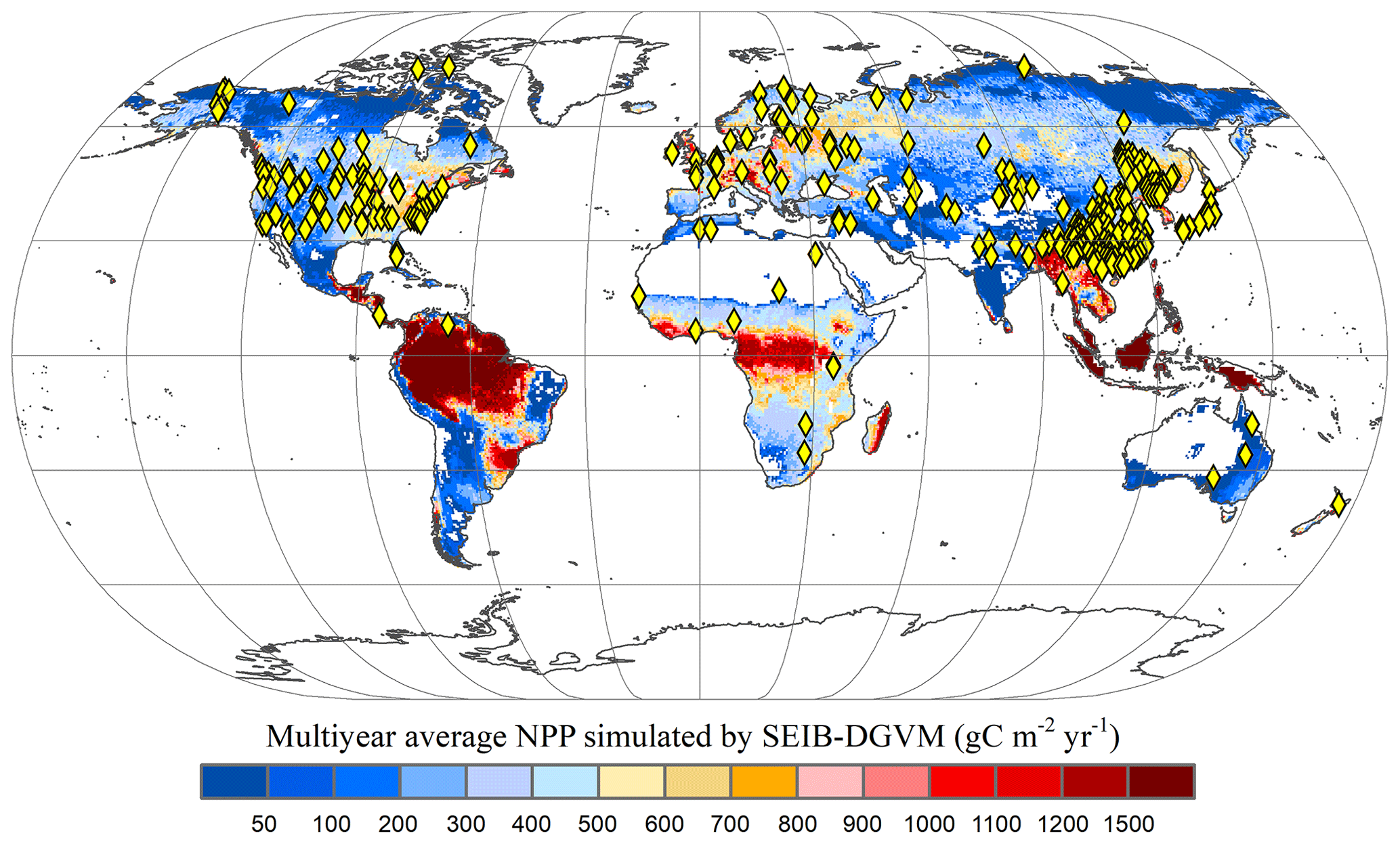
Figure 2 Multiyear average NPP simulated by SEIB-DGVM and EMDI global site distribution. Yellow rhombuses indicate the monitoring stations of the EMDI.

However, in situ observations are sparse for global spatiotemporal validation. Therefore, we used the MOD17A3 products to further verify the simulated potential NPP in the 21st century. These data were collected by the Moderate Resolution Imaging Spectroradiometer and are some of the most widely used data to assess the accuracy of global model simulations (Gulbeyaz et al., 2018). The natural vegetation zones refer to the hypothetical condition that would prevail in an assumed absence of anthropogenic activity, but under historical climate fields (Erb et al., 2018; Haberl et al., 2014). The potential NPP is defined as the assimilated carbon stored in natural vegetation without the disturbance of anthropogenic activities (Erb et al., 2018).

In order to distinguish the distribution of vegetation grid cells without anthropogenic disturbance, we obtained global land cover types in the period 2001–2015 from MCD12C1 (Table A1). We included grid cells whose largest vegetation component was evergreen needleleaf forest, evergreen broadleaf forest, deciduous needleleaf forest, deciduous broadleaf forest, mixed forest, closed shrublands, open shrublands, woody savannas, savannas, or grasslands. Other grid cells were excluded from our analysis.

Some of the grid cells covered by grassland were grazed by livestock, leading to the decrease in NPP of grass PFTs. There is a weak anthropogenic disturbance in rangeland, while managed pasture is intensely grazed by livestock. To remove pasture area with strong anthropogenic disturbance, we obtained land use forcing data from Land-Use Harmonization (LUH2) to map the distribution of managed pasture data from 2001 to 2015 (Hurtt et al., 2020). As shown in Fig. A5, grassland in eastern Asia, western Europe, south-central Africa, and western South America was severely affected by grazing. To exhibit the disturbance of managed pasture, we calculated the mean fraction of managed pasture within the corresponding 0.5^∘ grid unit. When the fraction of managed pasture is over 10 %, the grid cell was considered to be affected by managed pasture. To reduce the interference effects of livestock grazing, we first removed the grid cells affected by managed pasture. Then, we map the distribution of natural vegetation grid cells without anthropogenic disturbance (Fig. A6). This exclusion method is only used for potential NPP comparison.

3 Results and discussion

3.1 Evaluation of SEIB-DGVM

Figure 3 illustrates the comparison between model-simulated and observed multiyear mean NPP during 1916–1999. The determined coefficient (R²) between EMDI, observed and estimated multiyear average NPP of 669 in situ observations is 0.54, which is significant at the p=0.01 level. The slope of the regressed line is 0.70 during the 20th century.

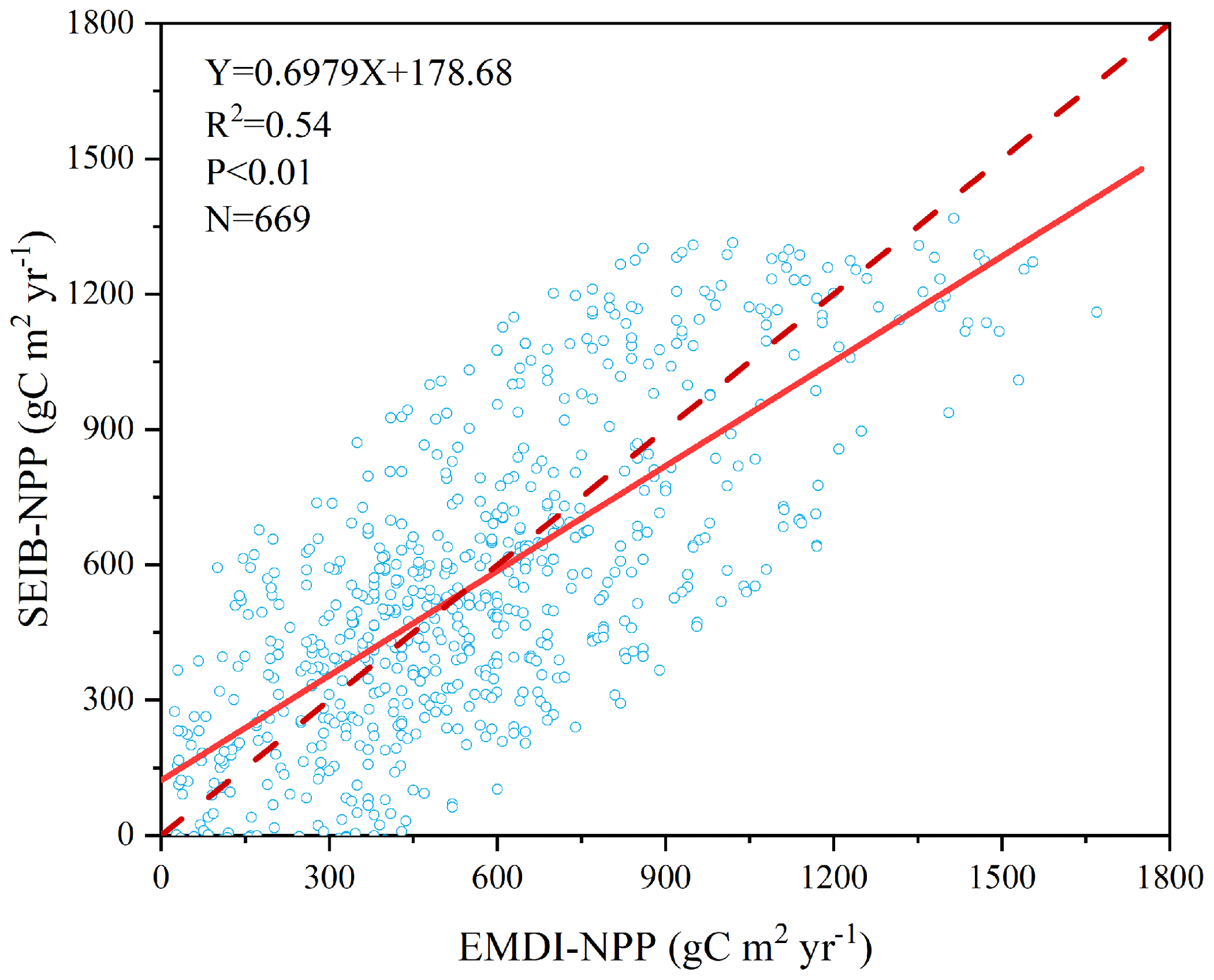
Figure 3 Comparison of multiyear average NPP calculated by SEIB-DGVM and EMDI for the 20th century. The solid line is the best-fit curve, and the dashed line represents a perfect correspondence in the results of the two.

Based on the land cover type dataset from 2001 to 2015, we obtained NPP-MOD17A3 data in natural vegetation zones without anthropogenic disturbance in the same period. Figure 4 shows that the modelled NPP from the SEIB-DGVM exhibited a high degree of consistency with the NPP-MOD17A3 data in natural vegetation zones over the period (R²=0.63, p<0.05). The general spatiotemporal agreement between the simulated NPP derived from SEIB-DGVM with in situ observations and derived from satellites reveals that it is reasonable to use the SEIB-DGVM simulations to evaluate the same mechanisms controlling global potential biomass carbon stocks of vegetation.

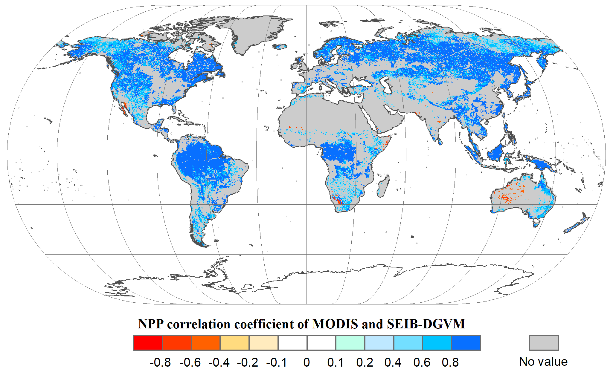
Figure 4 Spatial patterns in the potential NPP correlation coefficients (P<0.05) between SEIB-DGVM and MODIS between 2001–2015. These data were used to validate SEIB-DGVM.

Finally, the modelled result of potential vegetation biomass carbon stock was compared with current existing data from the literature and state-of-the-art datasets. Figure 5 shows that the modelled results are within the range of potential carbon stocks, which indicate that the SEIB-DGVM reliably simulated the carbon stock dynamics.

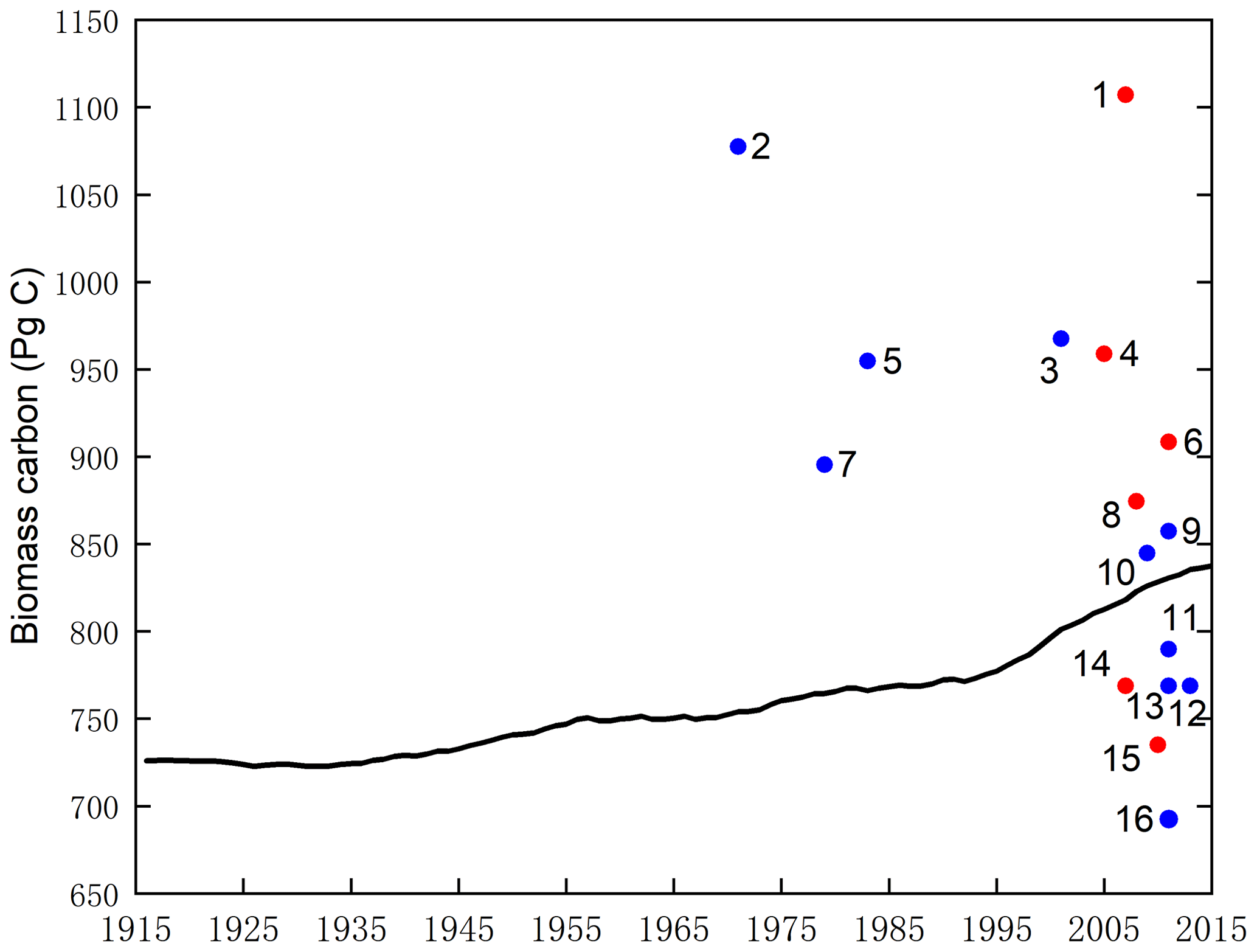
Figure 5 Estimates of the potential vegetation biomass carbon stock from the literature (blue plot), state-of-the-art datasets (red plot), and this study (black line). Datasets are from the following studies: (1) Erb et al. (2018, 2007), (2) Bazilevich et al. (1971), (3) Saugier et al. (2001), (4) Erb et al. (2018) and Bartholome and Belward (2005), (5) Olson et al. (1983), (6) Erb et al. (2018) and Pan et al. (2011), (7) Ajtay et al. (1979), (8) Erb et al. (2018) and Ruesch and Gibbs (2008), (9) Kaplan et al. (2011), (10) Shevliakova et al. (2009), (11) Kaplan et al. (2011), (12) Pan et al. (2013), (13) Prentice et al. (2011), (14) Erb et al. (2018, 2007), (15) Erb et al. (2018) and West et al. (2010), (16) Hurtt et al. (2011).

3.2 Enhanced carbon stocks and their fractions

We distinguished the changes in LVBC and WVBC from total vegetation carbon stocks. The historical temporal trends over the period are shown in Fig. 6a. The potential vegetation carbon stock exhibits a net increase of 119.26 ± 2.44 Pg C in the last century (±2.44 represents intra-annual fluctuation in carbon stock, which is the difference between the maximum value and minimum value of the carbon stock within the year). Based on Pearson correlation analysis, this increasing trend of annual average carbon stock exhibits a robust agreement with the dramatic increase in atmospheric CO₂ concentration (R²=0.9677, p<0.001), suggesting that the carbon stock is strongly affected by CO₂ fertilization. Meanwhile, the positive correlation between the carbon stock and CO₂ generally extends across LVBC (R²=0.9669) and WVBC (R²=0.9622). After the value of the global terrestrial carbon stock and trends were partitioned among the vegetation functional classes, we see that LVBC increases by 116.18 ± 2.34 Pg C (or ∼15.60 %), which explains 97.42 % of the total carbon stock increasing trend and dominates the positive global carbon stock trend; WVBC also increases by 3.08 × 0.14 Pg C (or ∼18.03 %) over the past century.

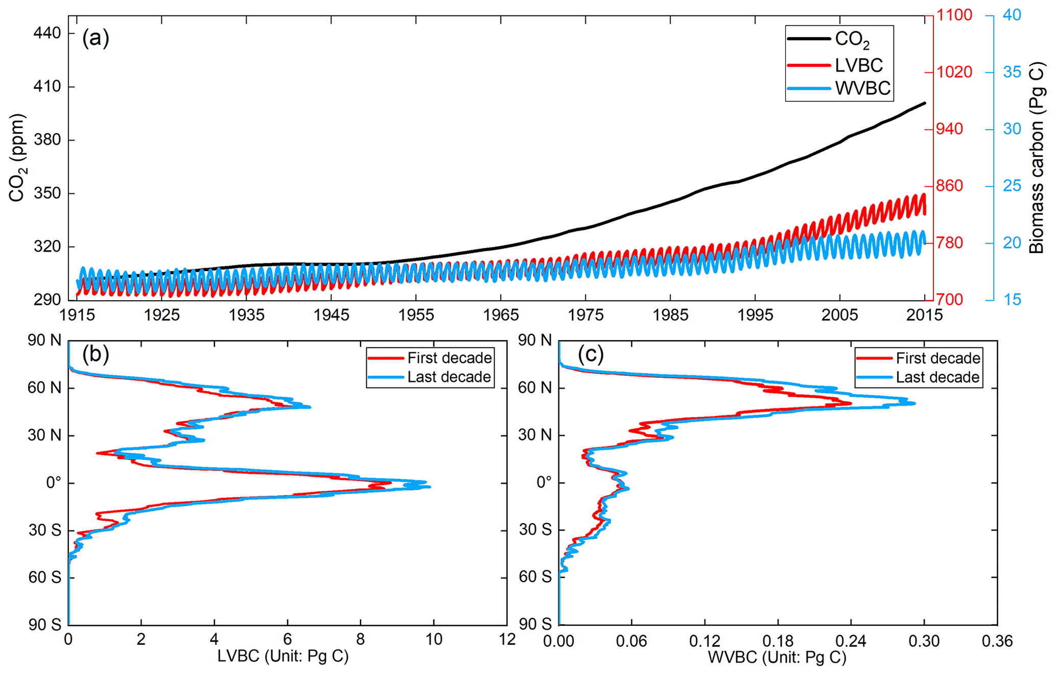
Figure 6 Global potential biomass carbon stocks of vegetation during the past 100 years. (a) The evolution of global potential biomass stocks (LVBC+WVBC), along with changes in biomass stocks that can be attributed to the variability and trend of LVBC and WVBC through the 20th century. The red line represents the monthly value of LVBC, the blue line represents the monthly value of WVBC, and the black line represents the annual value of CO₂ concentration. (b, c) Zonally averaged sums of the annual LVBC and WVBC for latitudinal bands during the first decade (1916–1925, red line) and the last decade (2006–2015, blue line) show the increased carbon stock capacity.

The global distributions of the decadal-average change in LVBC and WVBC are shown in Fig. 6b and c, respectively. The significant historical changes in climate and CO₂ enhance the carbon stock of the terrestrial ecosystem, and their positive influences are broadly distributed across a latitudinal north–south gradient. The latitudinal bands of increasing annual LVBC are mainly distributed at the tropical and boreal latitudes, which is consistent with Fig. 7b. The decadal and inter-annual variabilities in LVBC are dominated by the tropical and boreal zones, where large portions of which are highly productive (Ahlstrom et al., 2015; Poulter et al., 2014). Tropical LVBC dominates the long-term trend of global LVBC in the last 100 years. Compared with LVBC, the increase in tropical WVBC is light. There is a single peak in the spatial variation in annual WVBC (Figs. 6c and 7c). WVBC exhibits robust growth at most latitudes and increases mainly at boreal latitudes.

3.3 Spatial variability in estimated LVBC and WVBC trends

In Fig. 7a and b, total carbon stock and LVBC exhibited a significantly increasing trend in eastern South America, southern Africa, and northern Asia, while it declined in central North America, north-western South America, and central Africa. WVBC showed a more widely increasing tendency in North America, south-eastern South America, and Europe, while it had a decreasing trend in some zones of Asia. We find that the total carbon stock as well as the light- and water-gathering vegetation biomass carbon stocks over the period of 1916–2015 exhibited a remarkable spatial heterogeneity. Figure 7a shows that an increase in vegetation carbon stocks occurred over zones and global aggregate levels during the entire study period. About 57.39 % of the terrestrial grid cells exhibited an increase with a noticeable trend (p<0.05) in biomass carbon stock; 53.82 % of global grid cells possessed increases that were statistically significant at the p=0.01 level. To determine the contributions of each fraction (LVBC, WVBC) to the total change in the potential vegetation carbon stock, we partitioned and present the historical spatial and temporal patterns for each fraction separately (Fig. 7b, c). LVBC contributes 97.33 % of the incremental change in total carbon stock (116.18 × 2.34 Pg C), with about 51.32 % of the grid cells possessing a noticeable positive trend (p=0.01). Generally, spatial patterns of LVBC and the total carbon stock are consistent (Fig. 7a, b), which further supports the argument that LVBC dominates the trend in carbon stocks in most zones. Although the proportion of the total change in carbon stocks is small (2.58 % of total carbon stock increase), about 61.00 % of the land surface shows an increase in WVBC; of these terrestrial grid cells, 55.81 % was characterized by a significant p=0.01 increase.

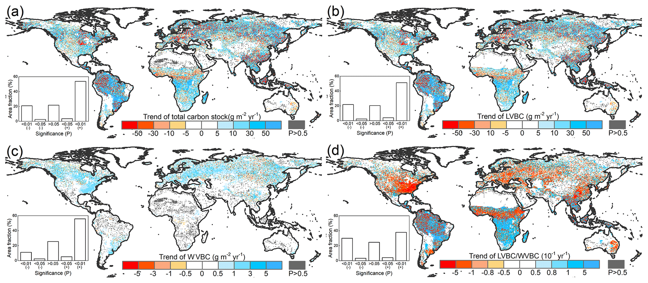
Figure 7 Spatial patterns in the trends of potential vegetation carbon stocks and their fractions from 1916 to 2015. Difference induced by changes in climate and CO₂ in terrestrial biomass carbon stock (a), LVBC (b), and WVBC (c) during the historic period 1916–2015. The blue bar indicates the significantly increasing trends, and the red bar indicates the significantly decreasing trends in carbon stocks. (d) Trend in the LVBC $/$ WVBC ratio from 1916 to 2015. The blue bar indicates significantly increasing trends in the ratio, and vice versa. The grey bar indicates that the trend is statistically insignificant (P>0.05). The sub-graphs show the significant test results. A “+” symbol indicates a positive trend, and vice versa.

Under the influence of a changing climate and CO₂ concentrations, there is a slight increase in the ratio of global LVBC $/$ WVBC; the rate of increase is 0.0171 yr⁻¹ in the last 100 years, which is significant at the 0.01 level (Fig. 7d). About 42.08 % of the terrestrial grid cells exhibit an increase with a noticeable trend (p<0.05) in the ratio of LVBC and WVBC; 37.95 % of global grid cells possessed increases that are statistically significant at the p=0.01 level. Meanwhile, 33.32 % of the land surface shows a significant decrease in LVBC $/$ WVBC; of these terrestrial grid cells, 30.06 % are characterized by a significant p=0.01 decrease. Grid cells with noticeable increases in the ratio of LVBC to WVBC are mainly located in southern Africa, central South America, and northern Eurasia. Negative trends in LVBC $/$ WVBC ratios are found in northern America, southern Europe, and tropical Africa.

3.4 Responses of LVBC and WVBC to environmental drivers

The responses of LVBC and WVBC to changes in climate and CO₂ are both positive at the global level (Fig. 8a, c), although zonally, they exhibit both negative and positive responses (Fig. 8b, d). Based on the results of factorial simulations and Mann–Kendall and Sen tests, CO₂ fertilization explains the largest proportion of the change in the carbon stock; about 82.45 % of the change in LVBC was positive (Fig. 8a), whereas 89.28 % of the change in WVBC was positive (Fig. 8c). In factorial simulation S2, the long-term trend of LVBC was 15.521 g C m⁻² yr⁻¹, and that of WVBC was 0.435 g C m⁻² yr⁻¹ in the period from 1916 to 2015 (Figs. A2a and A3a). The separately simulated LVBC and WVBC increased by 80.98 and 2.66 Pg C with increasing atmospheric CO₂ concentrations (from 301.73 ppm in 1916 to 400.83 ppm in 2015). The other climatic drivers (precipitation, temperature, radiation, humidity, and wind speed) remained at baseline values. While the increase or decrease in the carbon stock may be attributed to more than one driving factor, within any specified grid cell, the one with the highest positive or negative contribution is the dominant driver that consistently resulted in the highest increase or decrease in the carbon stock for that grid cell. The spatial pattern illustrates that CO₂ dominates the variability in LVBC in 7.28 % of the grid cells, including 1.21 % of the grid cells that exhibited a negative change and 6.07 % that exhibited a positive change (Fig. 8b). CO₂ dominates the variability in WVBC in 27.60 % of the grid cells, including 1.73 % of the grid cells that exhibited a negative change and 25.87 % of grid cells with a positive change (Fig. 8d). Under the effect of CO₂ fertilization, grid cells with increased trend in WVBC are mainly distributed at boreal latitudes (Fig. 6c). These trends are consistent with previous studies (Tharammal et al., 2019; Zhu et al., 2016; Keenan et al., 2016) in which positive trends occurred, especially for WVBC.

Figure 8 The proportion of changes in vegetation biomass carbon stocks attributed to driving factors. Ratios of the driving factors of CO₂ fertilization effects (CO₂), climate change effects (CLI), precipitation (Pre), temperature (Tem), and radiation (Rad) for LVBC (a) and WVBC (c) are calculated by the Mann–Kendall and Sen slope estimator statistical tests. Attribution of LVBC (b) and WVBC (d) dynamics to driving factors calculated as averages along 15^∘ latitude bands. At the local scale, the driving factors include CO₂, Pre, Tem, Rad, and other climate factors (OF). The fraction of global grid cells (%) that are predominantly influenced by the driving factors is shown at the bottom of the bar. The “–” symbol before the fraction indicates a negative effect of the driving factor on carbon stock, and vice versa.

Climate change induced by the greenhouse effect explains part of the increase in carbon stocks, but unlike CO₂ fertilization, climate has dramatic negative effects on some vegetated zones. Figure 8a illustrates that temperature is the largest climatic contributor to the change in LVBC (13.83 %, 2.572 g m⁻² yr⁻¹), followed by precipitation (8.51 %, 1.572 g m⁻² yr⁻¹) and radiation (−3.19 %, −0.649 g m⁻² yr⁻¹). The spatial distribution shows that temperature predominantly influences the change in LVBC (Fig. 8b), influencing over 27.56 % of the global vegetated grid cells, followed by precipitation (21.88 %) and radiation (20.67 %). Figure 8c shows there are negative contributions of precipitation to the change in WVBC at the global level (−2.76 %, −0.013 g m⁻² yr⁻¹) by precipitation. Temperature is the largest climatic contributor to the change in WVBC (15.36 %, 0.075 g m⁻² yr⁻¹), followed by radiation (−5.63 %, −0.027 g m⁻² yr⁻¹). Modelled WVBC trends based on the factorial simulations have similar spatiotemporal patterns to LVBC (Figs. A2 and A3), and the spatial patterns of light- and water-gathering carbon stocks show a significantly increasing trend in most of the boreal zones. In the Southern Hemisphere, the trends of WVBC are extensively statistically insignificant in all factorial simulations, and only a small proportion of grid cells show a significantly increasing trend. There is a significantly increasing trend in LVBC in south-central Africa and northern South America. The effects of temperature on WVBC are stronger than LVBC because temperature has a stronger effect on the metabolism process of root growth, dominating the turnover rate and the costs of maintenance respiration in root growth processes (Gill and Jackson, 2000). It should be noted that trends in the global carbon stock can be largely attributed to the influences of CO₂, precipitation, temperature, and radiation (Fig. 8). Nonetheless, at the zonal scale, the contributions of other factors should be considered, such as humidity and wind speed. The effects of these other factors dominate trends in LVBC in over 16.05 % of the grid cells that increased and 6.57 % of the grid cells that decreased. In the case of changes in WVBC, other factors were dominant drivers in over 14.75 % of the grid cells that increased and 3.57 % of the grid cells that decreased. Under the effect of climate, the variability in LVBC and WVBC is positive in most grid cells, promoting the noticeable increase in carbon stocks at boreal latitudes.

3.5 Constraints imposed by water limitations

Terrestrial water availability emerged as a key regulator of terrestrial carbon storage, by affecting the response mechanism of the vegetation carbon stock to changes in driving factors. As shown in Figs. 9 and 10, with the accumulated change in LVBC and WVBC in the period of 1916 to 2015 across the aridity index (i.e. an increase in available water), the magnitude and range in responses of LVBC density and WVBC density gradually increase. Based on the results of the historical simulation (Fig. 9), we find a positive relationship between LVBC and aridity index. In extreme water stress, the increase in LVBC tends to zero, and plants stop increasing their carbon storage. There is no obvious difference in the slopes of fitting curves between factorial simulations, which shows the robustness in the response of LVBC to the change in water stress. The pattern of the enhanced magnitude and range of variation in the WVBC density is unimodal with water stress gradient in all factorial simulations. With the increase in AI, the magnitude of change in WVBC increases at first and then decreases finally. The mitigation of water stress promotes WVBC increase, while excess surface water limits the response of WVBC to changes in climate and CO₂. These results reveal that the carbon stock increases stimulated by changes in climate and CO₂ are constrained by water availability. With increased warming, water limitations are expected to increasingly limit the carbon stock increase, especially in arid regions. To further reveal the controls of water limitation on the responses of inner carbon storages to each driver, we analyse the long-term variability in potential vegetation carbon stocks by means of factorial simulations for each hydrological region (Fig. 1). Figure A7b shows that the fluctuation range (the difference between maximum value and minimum value in each factorial simulation) of LVBC density across all factorial simulations is 1.202 kg C m⁻² in the hyper-arid regions for the 1916–2015 period. As shown in Fig. A7f, the fluctuation range of LVBC density in humid regions is 6.068 kg C m⁻² during the same period. In Fig. A8b, the maximum change in magnitude of WVBC density across all factorial simulations is 0.011 kg C m⁻² in the hyper-arid regions during the time of 1916–2015. In Fig. A8f, the maximum change in magnitude of WVBC density is 0.046 kg C m⁻² in humid regions during the same period. Compared with plants in arid regions, plants in humid regions show more dramatic responses to the stimulation from drivers' change. With a lessening of water stress (from hyper-arid to humid regions), the response magnitudes of the carbon stock to the changes in climate and CO₂ gradually become more noticeable. The robust pattern in the zonal average density of the carbon stock shows that terrestrial water limitations strongly regulate the enhanced magnitude of the carbon stock.

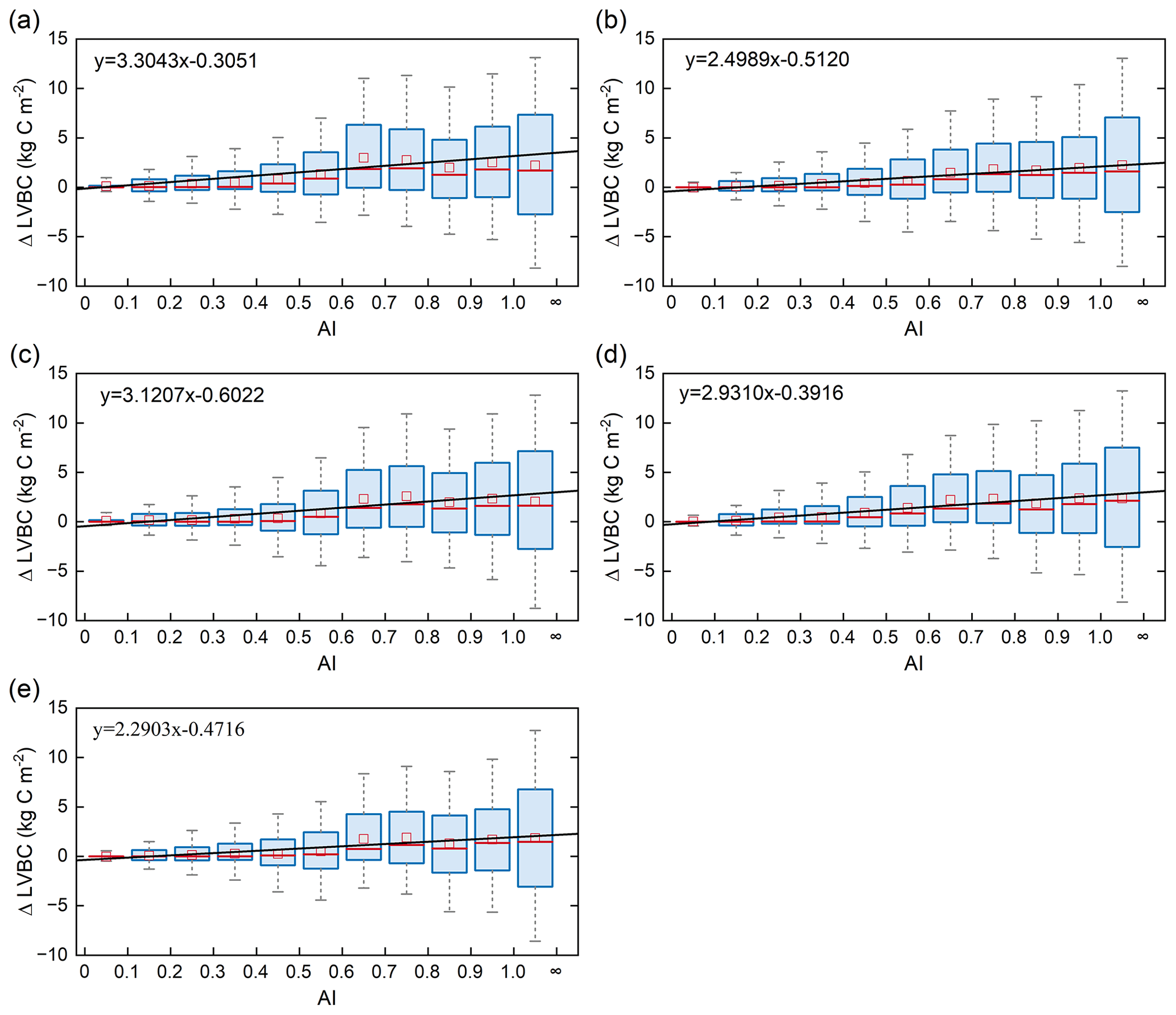
Figure 9 Relationships of the incremental change between AI and LVBC. Magnitude of change in LVBC in the historical scenario S1 (a), CO₂ in scenario S2 (b), CO₂+ precipitation in scenario S3 (c), CO₂+ temperature in scenario S4 (d), and CO₂+ radiation in scenario S5 (e). The range of the box is 25 %–75 % of values, the range of the whiskers is 10 %–90 % of values, the small red square is average value, the red line is the median line, and the black line is the fitted curve. Positive value of the y axis represents the magnitude of increased LVBC from 1916 to 2015 under water-limited conditions, and vice versa. AI of grid cells is calculated by multiyear average precipitation and multiyear average potential evapotranspiration in the period of 1916–2015. Categories of hydrological zones include hyper-arid (AI ≤ 0.05), arid (0.05 < AI ≤ 0.2), semi-arid (0.2 < AI ≤ 0.5), sub-humid (0.5 < AI ≤ 0.65), and humid (AI > 0.65).

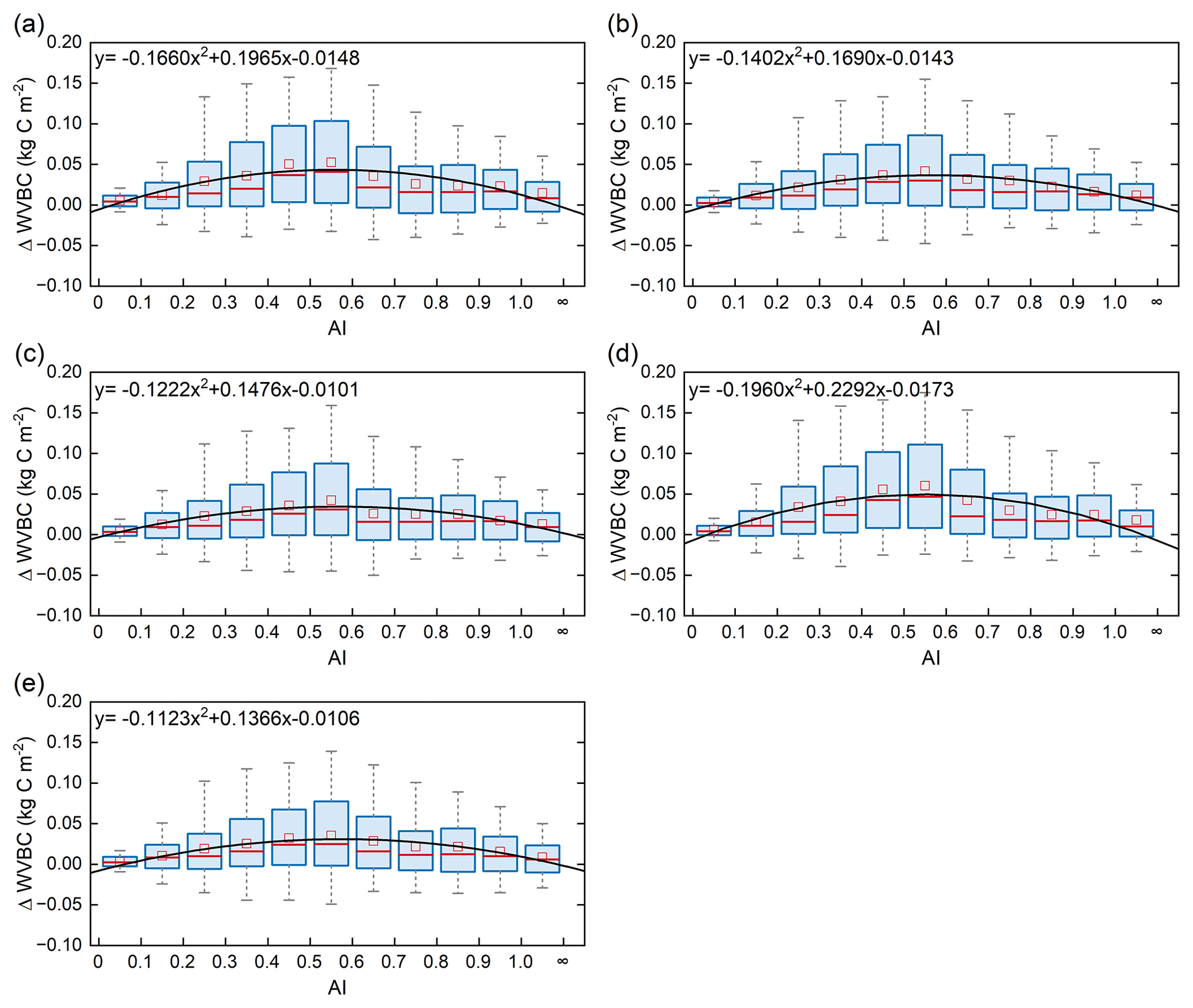
Figure 10 Relationships of the incremental change in AI and WVBC. Magnitude of change in WVBC in the historical scenario S1 (a), CO₂ in scenario S2 (b), CO₂+ precipitation in scenario S3 (c), CO₂+ temperature in scenario S4 (d), and CO₂+ radiation in scenario S5 (e). The range of the box is 25 %–75 % of values, the range of the whiskers is 10 %–90 % of values, the small red square is average value, the red line is the median line, and the black line is the fitted curve. Positive value of the y axis represents the magnitude of increased WVBC from 1916 to 2015 under water-limited conditions, and vice versa. AI of grid cells is calculated by multiyear average precipitation and multiyear average potential evapotranspiration in the period of 1916–2015. Categories of hydrological zones include hyper-arid (AI ≤ 0.05), arid (0.05 < AI ≤ 0.2), semi-arid (0.2 < AI ≤ 0.5), sub-humid (0.5 < AI ≤ 0.65), and humid (AI > 0.65).

Water limitations not only directly reduced the magnitude of the response in the two fractions' carbon stock (LVBC and WVBC) to changes in climate and CO₂ but also indirectly confined the response direction of each fraction's carbon stock by transforming vegetation structure and function. Figure 11 illustrates temporal variations in the carbon stock ratio within and between hydrological regions. From hyper-arid regions to humid regions, the fluctuation range of LVBC $/$ WVBC ratio significantly changes. The fluctuation magnitudes of LVBC $/$ WVBC in humid and hyper-arid regions are greater than those in other hydrological regions. Compared with plants in hyper-arid regions, plants in humid regions exhibit more significant responses to changes in climate and CO₂. Meanwhile, the long-term effects of driver changes have a remarkable influence on this carbon allocation pattern at the global level (Fig. 7d). Under the synergistic effect of drivers and water stress, the trends of light- and water-gathering vegetation carbon stock are upward in the past 100 years (Fig. 6). However, there is a difference in the increasing rate between LVBC and WVBC, resulting in a dramatic and complicated fluctuation in global LVBC $/$ WVBC ratio (Fig. 11a). Whereas LVBC decreases and WVBC increases in hyper-arid and arid regions (Figs. A7 and A8), causing a downward trend in the LVBC $/$ WVBC ratio, semi-arid regions see an increase in LVBC. So, the ratio of LVBC and WVBC shows a downward trend in these regions. LVBC in semi-arid regions shows upward tendency in the past years (Fig. A7d) because of the aridity mitigation. There is an upward trend in WVBC in semi-arid regions (Fig. A8d). Plants in semi-arid regions still utilize a tolerance strategy and allocate more non-structural carbon to water-gathering vegetation organs to resist water stress, resulting in the decline in the LVBC $/$ WVBC ratio. In humid regions, light- and water-gathering biomass carbon stocks both increased (Figs. A7 and A8). The proportion of LVBC increases more than that of WVBC for capturing more resources like CO₂ and radiation energy, leading to an increase in the LVBC $/$ WVBC ratio. The value of LVBC $/$ WVBC in S3 is higher than that in S4 and S5, which shows that precipitation makes a greater contribution to the change in LVBC $/$ WVBC ratio among meteorological factors.

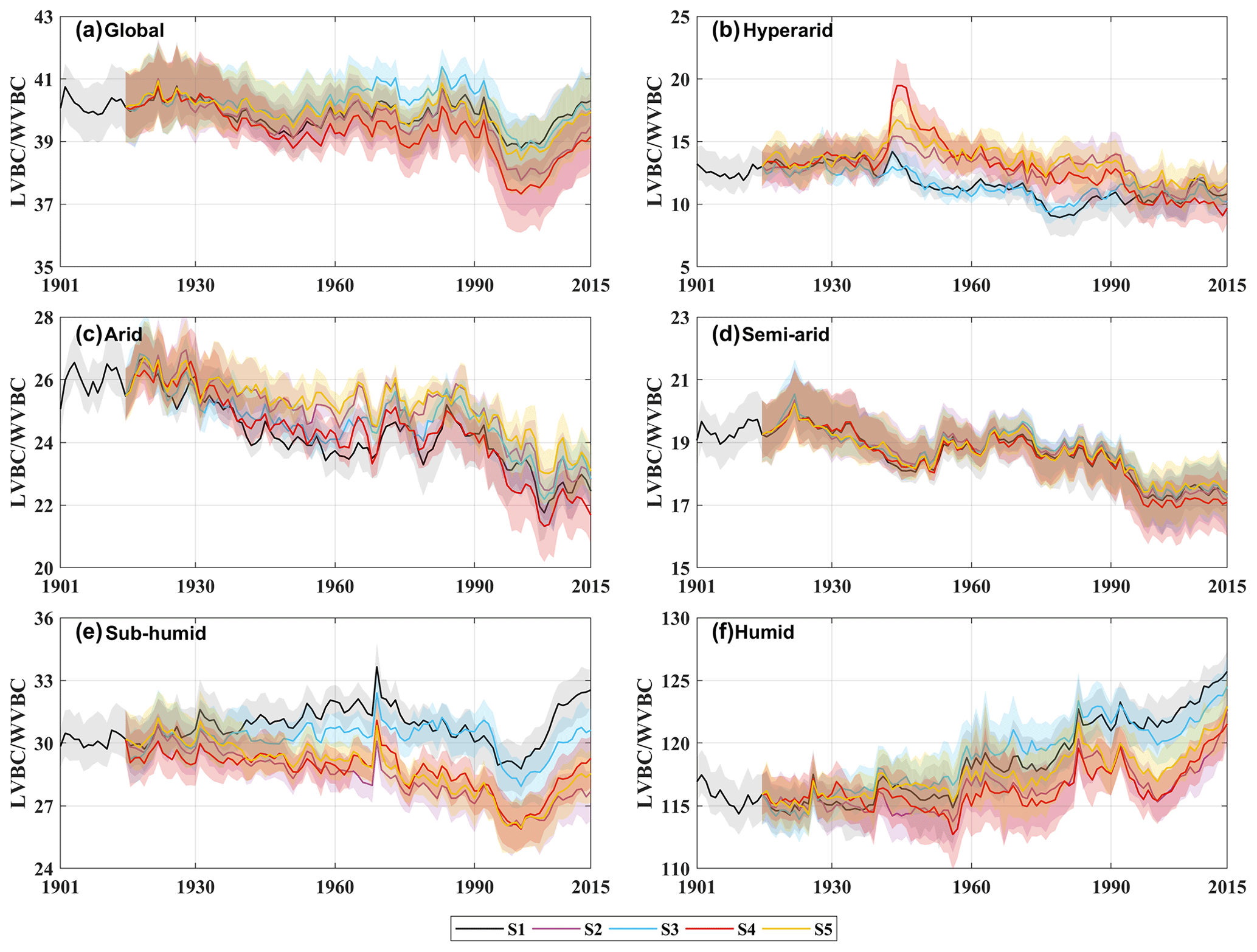
Figure 11 Temporal fluctuations in carbon stock dynamics in vegetation biomass in different factorial simulations. Black indicates historical factorial simulation from 1901–2015, green indicates the CO₂-driven factorial simulation, blue indicates the precipitation-driven factorial simulation, red indicates the temperature-driven factorial simulation, and yellow indicates radiation-driven factorial simulation. Uncertainty bounds are provided as shaded areas and reflect the intra-annual fluctuation (±1 s.d.). (a) Modelled trend of LVBC $/$ WVBC ratio in global area. (b–f) Modelled trend of the LVBC $/$ WVBC ratio in different hydrological regions (Fig. 1).

4 Discussions and conclusion

To understand the response of carbon storage potential and its inner biomass carbon stocks to environmental change, we conducted a series of factorial simulations using SEIB-DGVM V3.02. More importantly, we investigated the extent of the responses of carbon stocks to water limitations.

Over the past 100 years, there has been an ongoing increase in the carbon storage capacity of the terrestrial ecosystem from 735 Pg C in 1916 to 855 Pg C in 2015 (Fig. 6), which has slowed the rate at which atmospheric CO₂ has increased and may have mitigated global warming. These findings are consistent with the conclusions of research conducted at the local scale. For example, based on carbon flux data, Erb et al. (2008) suggested that the vegetation carbon stock in Austria increased from 1043 to 1249 Mt C (aboveground carbon stock growth was 1.059 Mt C yr⁻¹, and belowground carbon stock growth was 0.2 Mt C yr⁻¹) since industrialization. Le Noë et al. (2020) showed that increases in the carbon stocks and carbon density were the predominant drivers in the forest terrestrial carbon sequestration capacity in France from 1850 to 2015. Tong et al. (2020) also found a substantial increase in aboveground carbon stocks in southern China (0.11 Pg C yr⁻¹) during the period 2002–2017. However, these studies focused on zonal trends in total vegetation carbon stocks and did not investigate the extent of the response in vegetation carbon stocks partitioned between light- and water-gathering biomass. Our results show that the increase in carbon stock in light-gathering vegetation organs was much larger than that in water-gathering vegetation organs, and light-gathering biomass carbon stock dominates the historical trend of the terrestrial carbon stock. During the past decades, the global land surface has been greening because of the flux and storage of more carbon into plant trunks and foliage (Zhu et al., 2016). LVBC increases by 116.18 × 2.34 Pg C from 1916 to 2015, accounting for 97.42 % of the total carbon stock increase (119.26 × 2.44 Pg C). The long-term trends and spatial pattern of vegetation carbon stock predominated the variability characteristic of LVBC. The latitudinal bands of increasing annual change in LVBC are mainly distributed at tropical latitudes, a conclusion consistent with prior knowledge that tropical zones dominate carbon uptake and storage (Erb et al., 2018; Schimel et al., 2015). Biomass carbon allocation between light- and water-gathering vegetation organs reflects the changes in individual growth, community structure, and ecosystem function, which are important attributes in the investigation of carbon stocks and carbon cycling within the terrestrial biosphere (Hovenden et al., 2014; Fang et al., 2010; Ma et al., 2021). During the past 100 years, the ratio of LVBC $/$ WVBC showed a slight upward trend since LVBC increased relatively more than WVBC. The rate of increase is 0.0171 yr⁻¹, which is significant at the 0.01 level. To better absorb CO₂ and sunlight required for photosynthesis, vegetated regions are gradually covered by vegetation with higher plant height and wider leaf area, thereby adjusting their characteristic ecosystem functions (Erb et al., 2008).

Based on our factorial simulations (Fig. 8), the influences of CO₂ fertilization induce the most significant variation in the vegetation carbon stock. In addition, the responses of carbon stocks to the changes in climatic factors are obvious, particularly at the grid cell scale. Previous studies have pointed out that the variation in the terrestrial carbon stock caused by releasing or sequestering carbon is sensitive to anomalous changes in water availability and light use efficiency (Madani et al., 2020; Humphrey et al., 2018). At the grid cell scale, as shown in Fig. 8b and d, temperature, radiation, precipitation, and other climate factors (humidity and wind speed) dominate the long-term trend of carbon stocks over two-thirds of the global grid cells. At the global scale, climate factors explain 17.55 % and 10.72 % of the long-term trend in LVBC and WVBC, respectively (Fig. 8a and c). LVBC and WVBC variations driven by climate factors are ultimately offset by spatially compensatory effects, which dampens the response of the carbon stock to these factors at the global scale (Jung et al., 2017). Thus, contributions of precipitation and radiation to the variability in LVBC and WVBC are relatively low at the global scale, and the effects of humidity and wind speed on global carbon stock are minor. This spatially compensatory effect of climate change is consistent with a previous analysis (Zhu et al., 2016) which found that climate change explains only 8 % of the increasing trend in foliage carbon storage at the global level but that it dominates the trend over 28.4 % of the global land area. Results show that trends in temperature drive historical long-term trends in the potential carbon stocks, with faster increases and considerable variation occurring by grid cell. Thus, our results reveal that temperature dominates the long-term trends of carbon stock among climatic drivers, while a relatively strong compensatory effect exists in the global change in the carbon stock induced by precipitation, radiation, humidity, and wind speed.

By partitioning the trends of LVBC and WVBC into five hydrological regions (Fig. 1), we found that the long-term change in carbon stocks is tightly coupled to terrestrial water availability. These results indicate that vegetation in humid regions is responsible for most of the trend in global LVBC, while plants in semi-arid regions play a dominant global role in controlling the long-term trend in WVBC (Figs. 9 and 10). As water stress decreases, the magnitude and range in variation in LVBC gradually increase (Fig. 9), which suggests that limited water availability constrains the response magnitude of the changes in LVBC to changes in CO₂ and climate. The response pattern of WVBC growth to the increasing water availability is different from that of LVBC. Drought mitigation promotes the growth of WVBC. In sub-humid and humid regions, plants face low water limitations and intensified light competition and have to invest as much non-structural carbon as possible into leaf and trunk. This allocation scheme leads to the decreased investment of ΔWVBC in wet regions. The result is consistent with previous finding that plants reduce investment to roots in dense forests where aboveground competition for light is high (Ma et al., 2021). Moreover, we found that indirect effects of water limitation regulate increasing rate of each carbon pool. Although vegetation carbon stocks dramatically increase under the effects of climate and CO₂ changes, the increasing rate of LVBC is faster than WVBC in humid regions. Vegetation stores more biomass in aboveground plant organs (trunk and foliage) to gather light. Dryland plants decrease the LVBC $/$ WVBC ratios and store more biomass below ground to enhance the capture of water resources. Based on these results, we demonstrate that water limitations controlled the variable response of terrestrial vegetation carbon stocks.

Our findings are consistent with other reports about the impact of increasing water limitations on the terrestrial ecosystem. Based on observation from satellite remote sensing, Madani et al. (2020) found that the constraining impact of water limitation determines whether global ecosystem productivity responds positively or negatively to the changes in climate factors. Humphrey et al. (2021) found that increasing water stress limits the response magnitude of carbon uptake rates through a down-regulation of stomatal conductance and suggested that land carbon uptake is driven by temperature and vapour pressure deficit effects that are controlled by terrestrial water availability. Ma et al. (2021) found that plants increase investment into building roots in arid regions because the extent of water limitation there is exacerbated by global warming. Terrestrial hydrological conditions significantly affect the carbon cycle of terrestrial ecosystems, including carbon uptake, allocation, and stock. Terrestrial ecosystems utilize sensitive strategies to allocate and store biomass to adjust to local hydrological conditions. A significant conclusion is that water constraints not only confine the responses of vegetation carbon stocks to drivers but also constrain the proportion of biomass carbon stocks in light- and water-gathering fractions.

Distinguishing the response of carbon stock fractions estimated by SEIB-DGVM improves the understanding of the interactive impacts of terrestrial carbon and water dynamics. However, uncertainty still exists because of the limitations in the processes of modelling vegetation metabolism with SEIB-DGVM. Trunk biomass contains tree branches and structural roots (coarse roots and tap roots) (Sato et al., 2007), so the R $/$ S ratio of potential vegetation in factorial simulations is smaller than the R $/$ S of actual vegetation in observation stations. Root biomass only contains the fine root biomass, leading to an apparent underestimation in belowground organ biomass of trees and grasses compared with previous conclusions (Ma et al., 2021; Yang et al., 2010). Availability of nitrogen is a key limiting factor for vegetation growth, especially when higher CO₂ fertilization effects exist (Tharammal et al., 2019). The limitation could be alleviated by nitrogen deposition in most temperate and boreal ecosystems. The SEIB-DGVM experiments were conducted with a focus on documenting CO₂fertilization and climate change interactions; these experiments did not consider the influences of nitrogen deposition, which should cause an underestimation of the contributions of CO₂ fertilization to biomass production.

In summary, we evaluated SEIB-DGVM V3.02 and used this model to offer new perspectives on the response of vegetation carbon storage potential to changes in climate and CO₂. Our simulation results show that changes in CO₂, rather than climate, dominate the light- and water-gathering partitioning of the carbon storage potential. More importantly, we suggest that the impact of CO₂ fertilization and temperature effects on vegetation carbon sequestration potential depends on water availability and its impacts on plant stress. With increased global warming, water limitations are expected to increasingly confine global carbon sequestration and storage. Our findings highlight the need to account for terrestrial water limitation effects when estimating the response of the terrestrial carbon storage capacity to global climate change and the need for stronger interactions between those involved in vegetation model development and those in between the hydrological and ecological research communities.

Appendix A

Table A1 MCD12C1 legend and class descriptions.

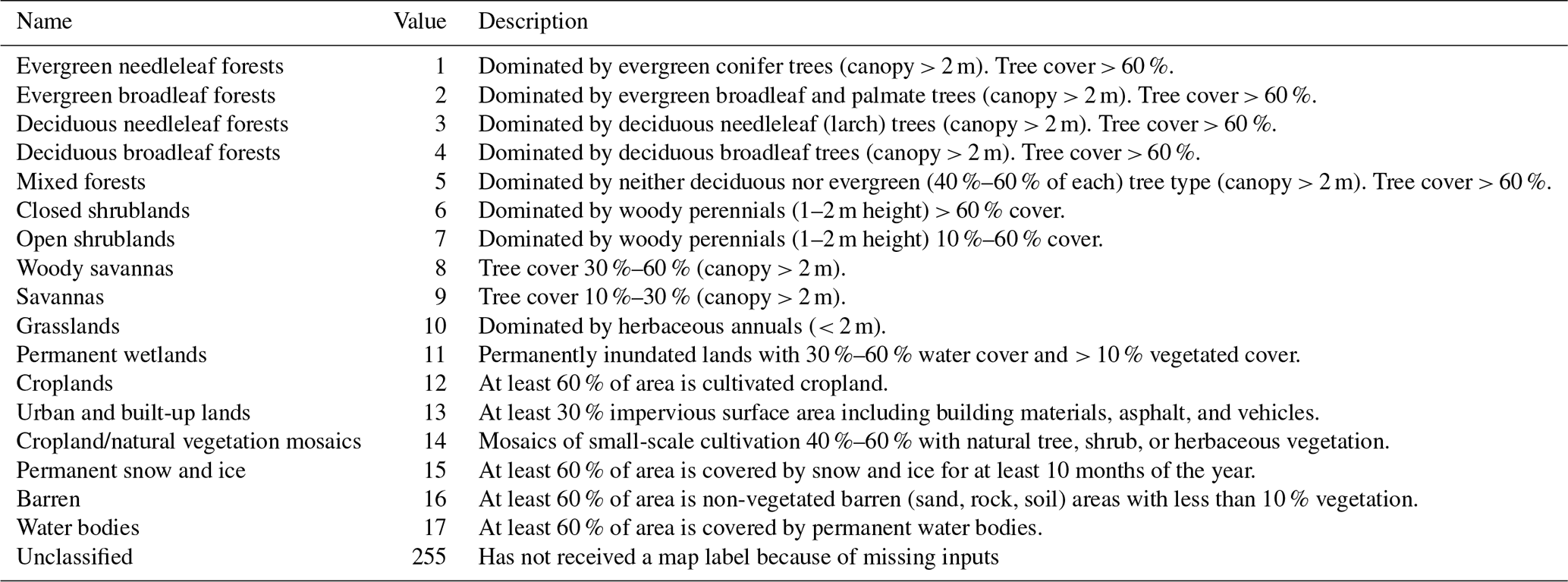
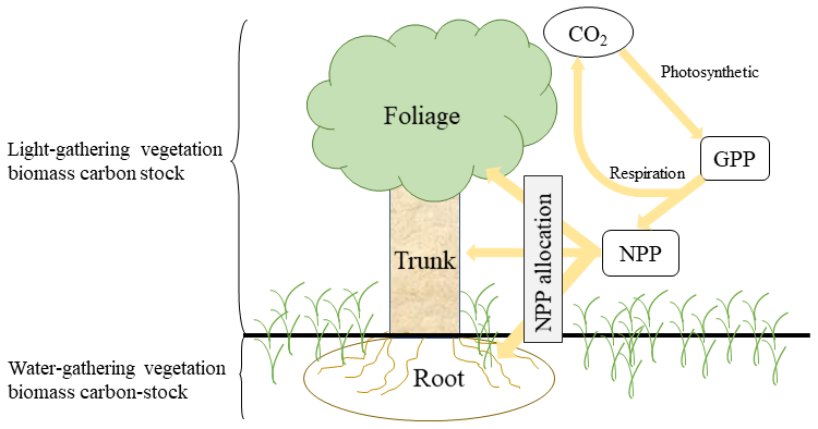
Figure A1 Schematic of ecosystem carbon cycle. Yellow arrow indicates carbon flux. Atmospheric CO₂ transitions into gross primary production (GPP) by photosynthesis. GPP is partitioned into respiration and net primary production (NPP). NPP is partitioned into three biomass carbon pools (foliage, trunk, and root).

Figure A2 Potential LVBC trend maps during the period of 1916 to 2015 under different factorial simulations. (a) CO₂ driving factorial simulation (S2), (b) CO₂+precipitation driving factorial simulation (S3), (c) CO₂+temperature driving factorial simulation (S4), and (d) CO₂+ radiation driving factorial simulation (S5). Positive values indicate increasing trends in the ratio, and vice versa. All results from the Mann–Kendall and Sen slope statistical tests correspond to the 95 % confidence interval.

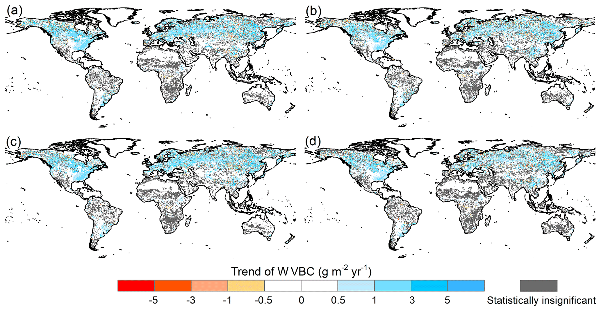
Figure A3 Potential WVBC variation trend maps during the period of 1916 to 2015 under different factorial simulations. (a) CO₂ driving factorial simulation (S2), (b) CO₂+precipitation driving factorial simulation (S3), (c) CO₂+temperature driving factorial simulation (S4), and (d) CO₂+radiation driving factorial simulation (S5). Positive values indicate increasing trends in the ratio, and vice versa. All results from the Mann–Kendall and Sen slope statistical tests correspond to the 95 % confidence interval.

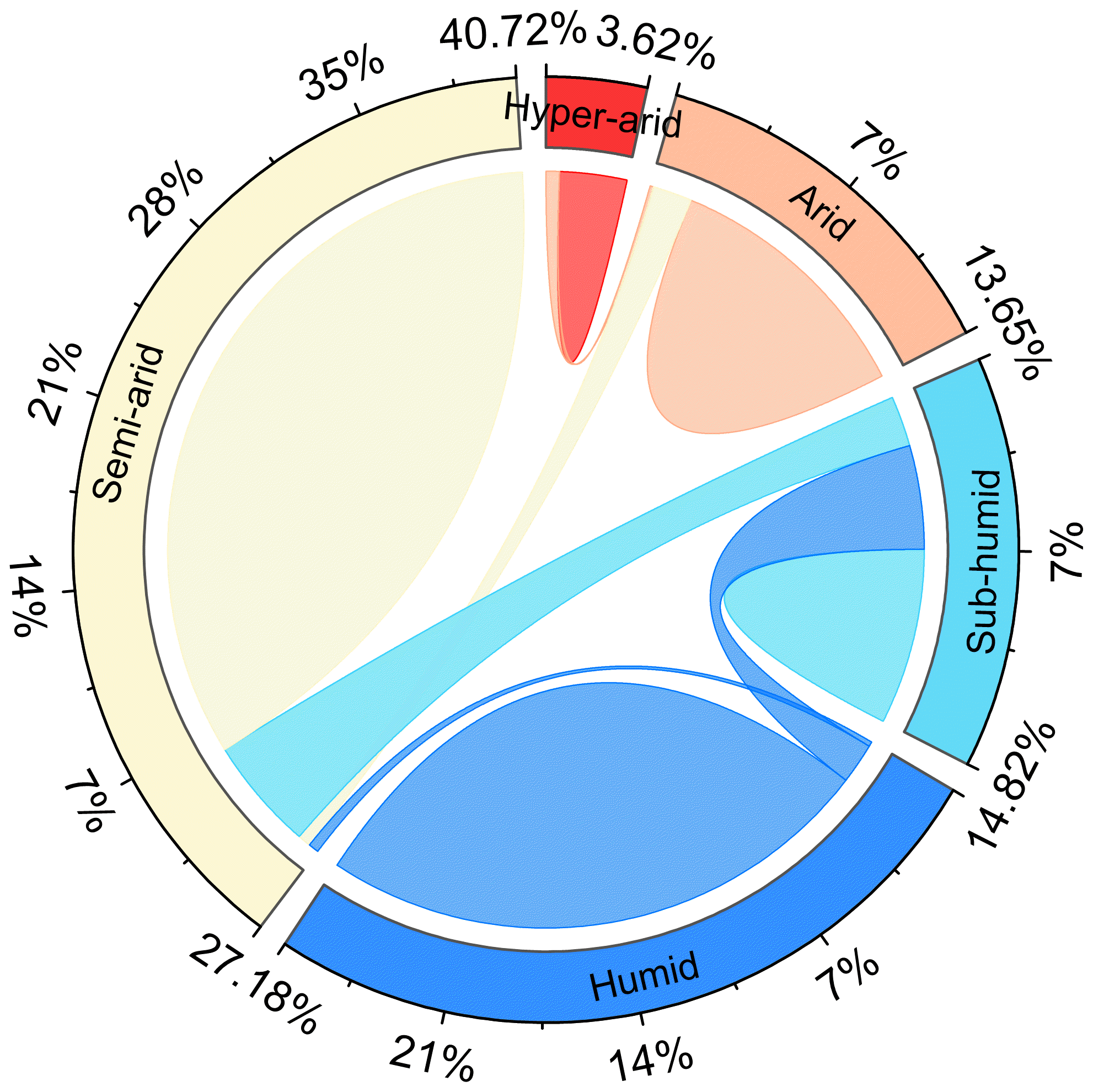
Figure A4 The shift in hydrological regions defined by the multiyear average AI index from the period of 1916–1945 to the period of 1986–2015. The outermost numbers represent the percentage of hydrological regions in 1916–1945.

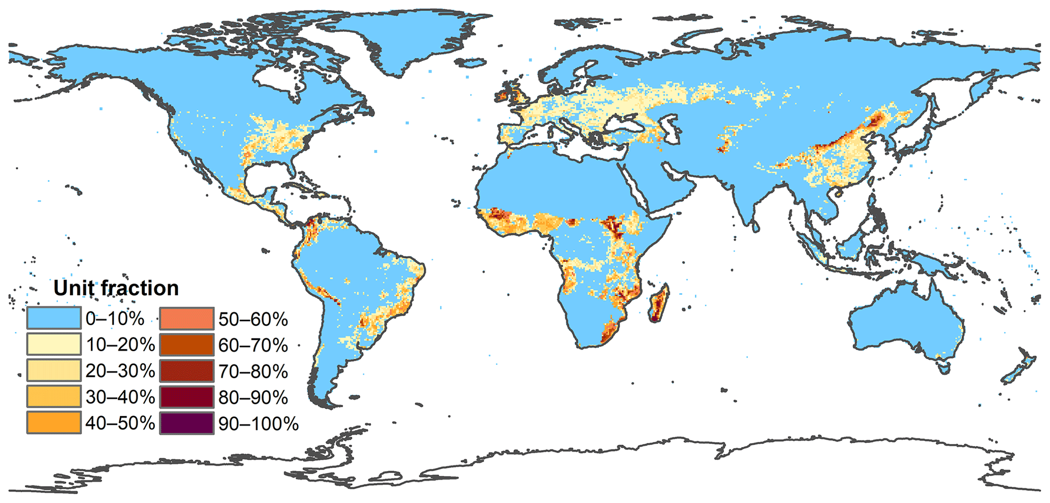
Figure A5 Spatial distribution of multiyear average fraction of managed pasture from 2001–2015 at 0.5 × 0.5 arcdeg resolution.

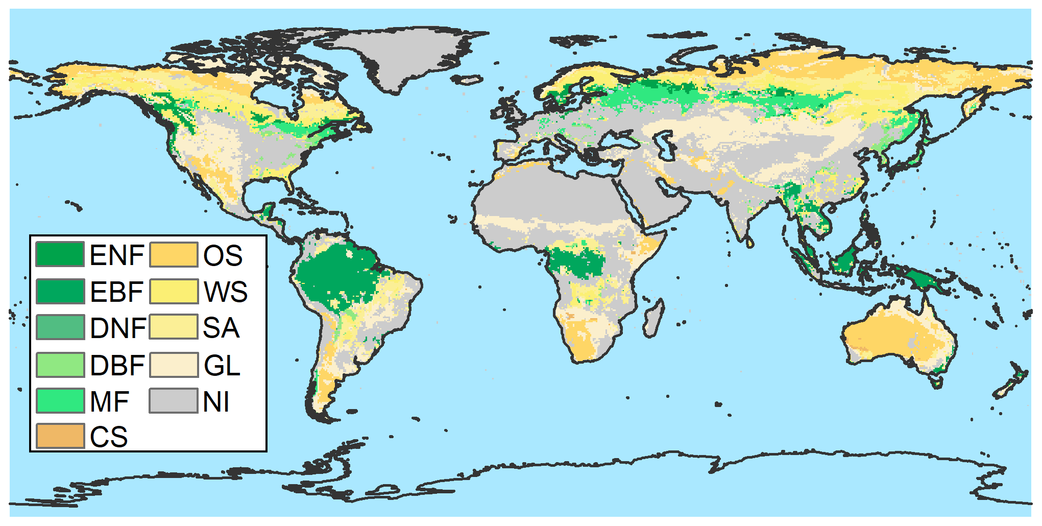
Figure A6 Map showing the largest vegetation component of each grid cell without anthropogenic disturbance from MCD12C1 and LUH2. ENF: evergreen needleleaf forest; EBF: evergreen broadleaf forest; DNF: deciduous needleleaf forest; DBF: deciduous broadleaf forest; MF: mixed forest; CS: closed shrublands; OS: open shrublands; WS: woody savannas; SA: savannas; GL: grasslands; NI: not included, which means the zone is not covered by vegetation without anthropogenic disturbance.

Figure A7 Trends in average density of potential LVBC. (a) Modelled trend of annually averaged LVBC globally. Modelled trends in annually averaged LVBC in hyper-arid regions (b), arid regions (c), semi-arid regions (d), sub-humid regions (e), and humid regions (f).

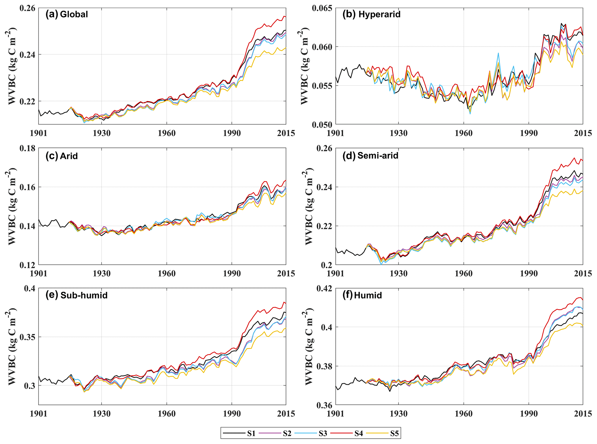
Figure A8 Trends in average density of potential WVBC. (a) Modelled trend of annually averaged WVBC globally. Modelled trends in annually averaged WVBC in hyper-arid regions (b), arid regions (c), semi-arid regions (d), sub-humid regions (e), and humid regions (f).