the Creative Commons Attribution 4.0 License.
the Creative Commons Attribution 4.0 License.
 | 31 Aug 2022
Observing system simulation experiments reveal that subsurface temperature observations improve estimates of circulation and heat content in a dynamic western boundary current
Colette Kerry
Moninya Roughan
Shane R. Keating
Western boundary currents (WBCs) form the narrow, fast-flowing poleward return flows of the great subtropical ocean gyres and are sources of rapidly varying mesoscale eddies. Accurate simulation of the vertical structure, separation latitude, and ocean heat content of WBCs is important for understanding the poleward transport of heat in the global ocean. However, state estimation and forecasting in WBC regions, such as the East Australian Current (EAC), the WBC of the South Pacific subtropical gyre, is challenging due to their dynamic nature and lack of observations at depth. Here we use observing system simulation experiments to show that subsurface temperature observations in a high eddy kinetic energy region yield large improvement in representation of key EAC circulation features, both downstream and ∼ 600 km upstream of the observing location. These subsurface temperature observations (in concert with sea surface temperature and height measurements) are also critical for correctly representing ocean heat content along the length of the EAC. Furthermore, we find that a more poleward separation latitude leads to an EAC and eddy field that is represented with far reduced error, compared to when the EAC separates closer to the Equator. Our results demonstrate the importance of subsurface observations for accurate state estimation of the EAC and ocean heat content that can lead to marine heatwaves. These results provide useful suggestions for observing system design under different oceanographic regimes, for example, adaptive sampling to target high energy states with more observations and low energy states with fewer observations.
- Article
(5345 KB) - Full-text XML
- BibTeX
- EndNote


Subtropical western boundary currents (WBCs) transport warm and saline waters towards the poles, and are key regions for eddy generation. Hence, they play a critical role in weather and climate, ecosystems, and biogeochemistry. They contribute to cross-shelf exchange with their adjacent coastal seas (Brink, 2016) and hence influence local blue economies (e.g. Li et al., 2017; Zeng et al., 2018). Given the proximity in location to populated coastlines and the dominant role in coastal ocean processes, characterizing and predicting WBCs and their related eddy fields is a subject of intensive observing and modelling efforts.
Due to the chaotic nature of mesoscale circulation, particularly WBCs, ocean models must be regularly updated through the incorporation of observations in order to correctly represent rapidly changing ocean conditions. Data assimilation (DA) is the combination of observations and a numerical model, such that the result is an optimal estimate of the ocean state (Moore et al., 2019). Due to the expense of observational oceanography and the vast nature of the ocean, there is strong motivation to optimize the results that are obtained from assimilation of sparse observations, and to provide insight into both ocean dynamics and guidance for designing optimized observing systems.
Observing system simulation experiments (OSSEs) provide a means by which the impact of assimilating different observations can be assessed using synthetic observations. In an OSSE, a model simulation is taken as representing the “true” state of the ocean that (unlike the real ocean) is completely known without error (Halliwell et al., 2014). Values are extracted from this simulation and realistic errors are added to represent synthetic observations. The impact of assimilating these synthetic observations can then be quantified by comparing the “truth” and the results of the OSSE forecast and analysis. A thorough examination of the impact of existing and hypothetical observing strategies on key dynamics of interest can then be conducted.
A key advantage of OSSEs is that they allow an assessment of future observational platforms and strategies, and so have been used for planning observational experimental design in many applications, for example: an Argo float array (Schiller et al., 2004) and moored instrument array in the Indian Ocean (Oke and Schiller, 2007; Ballabrera-Poy et al., 2007); glider deployments in the Western Atlantic (Halliwell et al., 2017) and the Solomon Sea (Melet et al., 2012); and Argo floats, drifting floats, and mooring arrays in the Atlantic (Gasparin et al., 2019). Kamenkovich et al. (2017) used OSSEs to determine the optimal number of autonomous floats to improve representation of biogeochemical variables in the upper Southern Ocean. Using an OSSE framework developed by Halliwell et al. (2014), various observing platforms in the Gulf of Mexico were investigated for improving hurricane prediction and oil spill response. Halliwell et al. (2015) found that deeper profiling expendable conductivity–temperature–depth (CTD) instruments better constrain upper ocean density (via observations of salinity), and hence ocean pressure and velocity. OSSEs have also been used to examine the impact of existing observation networks, for example, Lee et al. (2020) showed the relative effect of two serial CTD transects on representing flow patterns of the Kuroshio Current. OSSEs can also reveal the performance of the data assimilation system, such as in Moore et al. (2020), which showed the importance of choice of the assimilation window length.
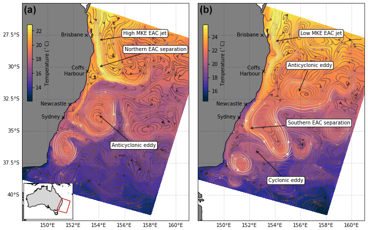
Figure 1Flow regimes of the EAC, highlighted in snapshots of sea surface temperature (colour) and circulation (arrows). The EAC flows southwards past Brisbane, generally as a coherent jet, before separating from the coast between Sydney and Coffs Harbour. (a) A higher mean kinetic energy of the EAC jet generally leads to more northern EAC separation, while (b) a lower mean kinetic energy in the EAC jet generally leads to more southern EAC separation (Li et al., 2021a). Flow instability leads to the generation of cyclonic and anticyclonic eddies. The background is coloured for model sea surface temperature and the streamlines indicate the concurrent surface circulation. Inset in (a) shows model domain in red outline.
In this study, we assess the relative impact of various observational platforms on the representation of the East Australian Current through an OSSE framework. The East Australian Current (EAC), like other WBCs, flows adjacent to the continental shelf, has strong currents, and is characterized by the poleward transport of warm and salty tropical waters. However, unlike other WBCs, as the EAC flows offshore, it does not form an extended inertial jet with pseudo-regular formation of eddies from the meandering current as in the Kuroshio Current (Kawabe, 1995) or the Gulf Stream (Richardson and Knauss, 1971). Instead, the EAC can be described as a “shelf-following” jet, which separates from the continental shelf to feed a poleward and eastward flowing eddy field of anti-cyclonic (counter-clockwise rotation with a warm core) and cyclonic (clockwise rotation with a cold core) eddies (Fig. 1). The latitude of separation varies northward and southward of the mean, typically between 31–32∘ S (Cetina-Heredia et al., 2014), and has been shown to be linked to the mean kinetic energy of the EAC jet upstream (Li et al., 2022a). The location of the EAC jet, along the continental shelf break from approximately 25∘ S (north of Brisbane) to 30∘ S–32.5∘ S (Coffs Harbour to north of Newcastle), and the subsequent eddy field which stretches south to Tasmania and eastward towards New Zealand are shown in Fig. 1. Key outstanding questions about the EAC focus on the observed warming of the EAC (Malan et al., 2021), the more frequent and intense nature of marine heatwaves (MHWs) in the EAC (Oliver et al., 2018) and their subsurface structure (Elzahaby and Schaeffer, 2019; Elzahaby et al., 2021), and changes to upper ocean heat content in the EAC (e.g. Li et al., 2022a). These questions are also relevant for analogous WBC systems that have been shown to be warming 2–3 times the global average (Wu et al., 2012). As well as understanding long-term change, there is a strong desire to improve short-term prediction, which is important for extreme weather events, search and rescue, oil spill response, and navigation. Future observing systems will have to be designed to target these key WBC uncertainties, but in a cost-effective manner.
Compared to other WBCs, the EAC is relatively well-observed (Roughan et al., 2015; Todd et al., 2019); however, these observations are expensive and require significant person-hours to obtain. Yet, optimizing the impact of different observations on the EAC has only recently seen dedicated research effort. Kerry et al. (2018) used DA methods to highlight that observations in regions of high natural variability contribute the most to constraining model solution, while Siripatana et al. (2020) showed the strong positive impact that high frequency radar and subsurface observations had on improving representation of the subsurface structure of the EAC. In this study, we employ a time-dependent, variational DA scheme to a shelf-resolving model of the EAC system and assess how various synthetic data streams impact estimates of key EAC features. In particular, we have chosen to examine the role of sea surface height (SSH), sea surface temperature (SST), and subsurface temperature observations in improving the simulation of prominent EAC flow features, the vertical and spatial heat and velocity distributions, and ocean heat content. Subsurface observations similar to those measured by eXpendable BathyThermographs (XBT) are systematically added in separate OSSEs to show the value of each observation platform in the absence or presence of the other subsurface observations. The impact of data from a range of observation platforms on correctly estimating the ocean state are also examined within different EAC separation regimes. In Sect. 2, the model setup and framework of the OSSEs are introduced, while Sect. 3 compares how each OSSE performs across a series of key metrics. Section 4 discusses the impact of assimilating observation on the simulation of EAC dynamics, the representation of ocean heat content, the influence of EAC separation latitude on state estimates (for example, representation of circulation and velocity), before finishing with recommendations for future observing system design for this dynamic WBC.
2.1 Data assimilating model
This study uses a numerical ocean model configuration of the Regional Ocean Modeling System (ROMS v3.9 ROMS/TOMS Framework: 3 March 2020) and employs the four-dimensional variational data assimilation (4DVar) framework, using an updated setup of Kerry et al. (2016). ROMS is a finite-difference method ocean model that solves the primitive equations on a horizontal grid with a terrain-following vertical coordinate. The model domain, with bathymetry sourced from the Geoscience Australia 50 m multibeam survey (Whiteway et al., 2009), extends from 27–38∘ S, over ∼ 700 km offshore, and is rotated by 20∘ so as to approximately align the grid parallel to the coastline (Fig. 1). Horizontal resolution is 2.5 km over the continental shelf and slope, and linearly increasing to 6 km in the deep ocean, with the 30 vertical s-coordinate layers with increased resolution in the surface and bottom boundary layers.
Lateral forcing conditions are taken from BRAN2020 (Chamberlain et al., 2021), comprising currents, temperature, and salinity. Surface forcing conditions are enforced with a bulk flux formulation (Fairall et al., 1996) using daily atmospheric fields from the Australian Bureau of Meteorology's ACCESS reanalysis (Puri et al., 2013). This model has been used previously for a number of studies, and further details on validation, forcing, and nudging conditions are given in Kerry et al. (2016), Li et al. (2022a), and Li et al. (2021a).
The DA scheme is the same as used in Kerry et al. (2016) and Kerry et al. (2018), namely an incremental strong constraint 4-dimensional variational scheme (IS4D-VAR; e.g. Moore et al., 2011b). This scheme increments the model initial conditions, boundary conditions, and surface forcing such that the difference between the model solution and observations is minimized, in a least squares sense, while considering errors in both. This minimization is performed over an assimilation window (in this case, 5 d) and, given the time-dependent nature of the technique, observation impact can be far-reaching, both upstream and downstream, and forward and backward in time (e.g. Kerry et al., 2018). We chose 15 inner loops to reduce the cost function, based on previous work of Kerry et al. (2016), who showed that this number of inner loops achieved an acceptable reduction with a reasonable computational cost. Similar cost function reduction is achieved for all OSSEs, with a time-mean ratio of final to initial cost function ranging between 0.73 to 0.80.
Background quality control was applied to eliminate observations that are poorly represented, following the method described in Moore et al. (2013). Only observations that satisfy are assimilated, where di is the innovation, the quality control parameter α=4, and σb and σo represent the prior background and observation errors. In all OSSEs, about 20 % of SST observations were rejected by this criteria while all of the SSH observations were assimilated. For the subsurface XBT observations, all observations were used for the single transect OSSEs, while in XBT-N+S, between 20 %–40 % of observations were rejected due to the innovation being too large. This method has been applied in several other recent 4DVar studies (Levin et al., 2021; He et al., 2022).
The simulations herein are performed over the period November 2011–January 2013. This period is chosen as a representative period for several key metrics (see Sect. 2.2) and also coincides with other studies (Kerry et al., 2016). All OSSE simulations are conducted with the model setup described here.
2.2 Assessment of the free-running simulation
A free-running (non-DA) simulation is required for comparison against (as the reference state) and to provide synthetic observations within the OSSE framework. We use a free-running simulation for the same period of time as the OSSEs, and the model configuration is identical to that used to produce longer-term simulations of the EAC system. These longer-term simulations have been demonstrated to produce an accurate representation of the mean and variability of the EAC circulation (Kerry and Roughan, 2020), which we further demonstrate with the mean kinetic energy (MKE) and eddy kinetic energy (EKE). The distribution of MKE and EKE (see Sect. 2.5) in the free-running model configuration is robust compared to satellite-derived estimates from AVISO (Archiving, Validation and Interpretation of Satellite Oceanographic Data) altimetry (Kerry et al., 2016; Li et al., 2021a). A variety of similar configurations have been used in previous studies to examine sub-mesoscale circulation (Kerry et al., 2020a), EAC seasonal variability (Kerry and Roughan, 2020), interannual variability and energy conversion (Li et al., 2021a), eddy-shelf interactions (Malan et al., 2021), and drivers of change in ocean heat content in the EAC southern extension (Li et al., 2022a). Additionally, the aforementioned EAC model provides boundary conditions for high-resolution nested studies (e.g. Ribbat et al., 2020; Roughan et al., 2022; Li et al., 2022b).
The free-running simulation uses surface forcing from the Bureau of Meteorology Atmospheric high-resolution regional reanalysis for Australia (BARRA-R; Su et al., 2019) and lateral boundary forcing from BRAN2020 (see above). Further details of the free-running simulation configuration are given in Kerry and Roughan (2020) and Li et al. (2021a). We refer to this 1-year free-running simulation as the “reference state”.
Li et al. (2021a), using a near identical configuration, showed that the sea surface MKE field matches well with AVISO satellite-inferred sea surface height observations for their long-running 1994–2016 simulation – lending confidence to how our model configuration is able to represent real conditions. The chosen 12-month period of the reference state also displays oceanographic conditions that match the long-term mean values (e.g. Li et al., 2021a), as shown in comparisons of spatial mean EKE and volume transport between the reference state and the mean values of these same quantities from the long-running simulation (Fig. A1). The reference state volume transport varies between 0 and 61 Sv (with a mean of 18 ± 15 Sv southwards), which compares favourably to the long-term (1994–2016) mean and standard deviation in volume transport of 21 ± 14 Sv (see Fig. A1a). Likewise, the time-mean EKE of the whole domain for the reference state (0.12 ± 0.027 m2 s−2) matches well to the long-term mean and standard deviation in EKE of 0.12 ± 0.028 m2 s−2 (see Fig. A1b). Together, these metrics, which represent the upstream EAC and downstream eddy field, show that the time period chosen is representative of the conditions in the EAC over the recent decades.
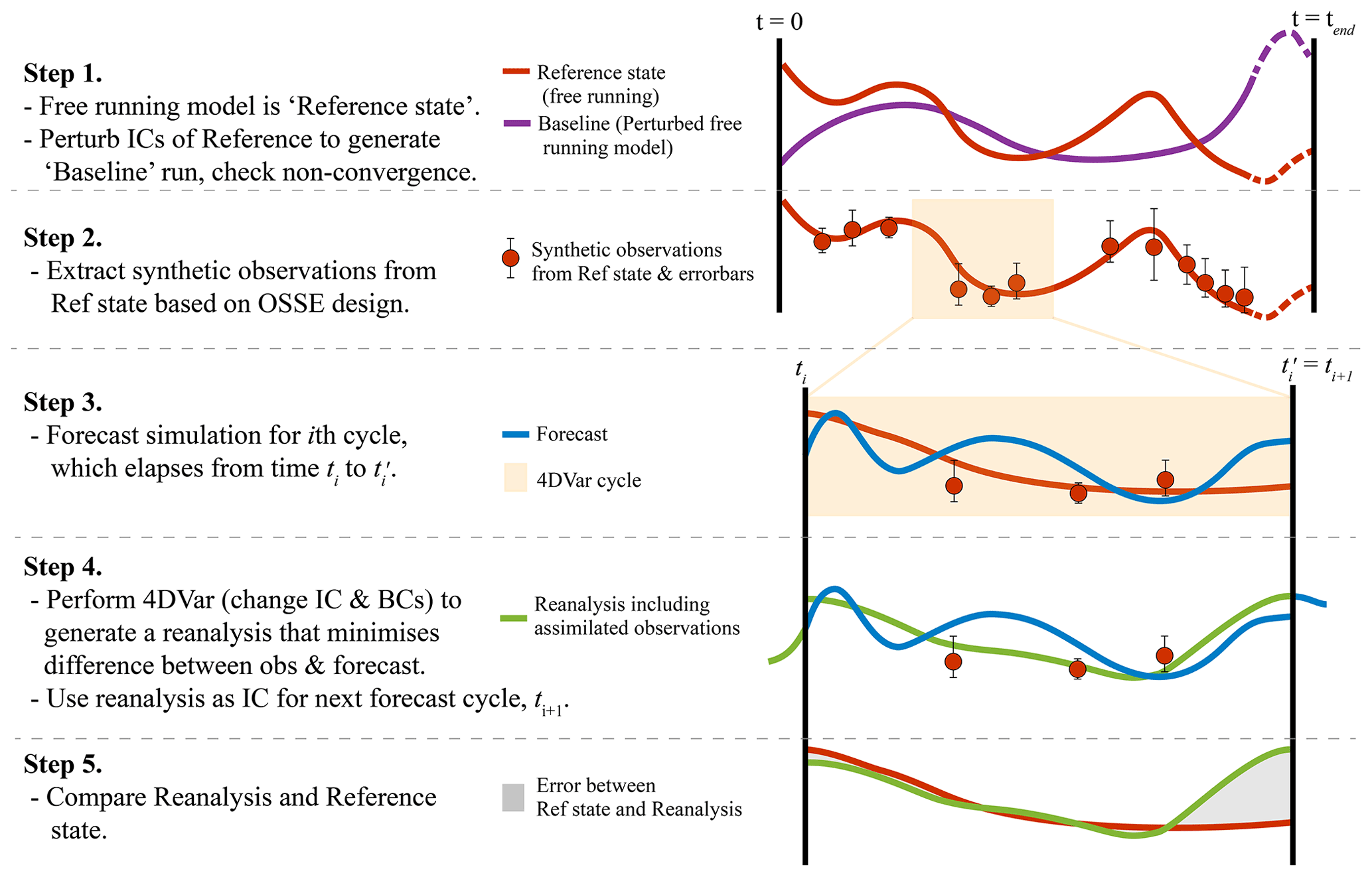
Figure 2The steps taken for conducting and assessing an OSSE using 4DVar are shown schematically.
2.3 The OSSE framework
A typical OSSE is conducted by comparing a free-running and data-constrained simulation, where the data constraints are values taken from the free-running simulation. We demonstrate our OSSE framework in the schematic shown in Fig. 2. The first step is simulating a free-running experiment for a set period of time (the reference state; step 1 in Fig. 2). A separate experiment, forced identically to the reference state but with perturbed initial conditions (see details of perturbation below), can also be simulated (“baseline” simulation; step 1 in Fig. 2). By comparing the baseline simulation to the reference state, the non-convergence of the initial conditions can be assessed. If the initial conditions provide a sufficient perturbation, then this will be used to perturb the start of each OSSE. Ocean conditions can be extracted from the reference state to form the synthetic observations (step 2 in Fig. 2), and the forecast is generated for the ith cycle (Step 3; Fig. 2). A reanalysis (with the perturbed initial conditions) is generated through assimilation of the synthetic observations into the forecast cycle, such that differences between the synthetic observations and the free-running forecast are minimized (Step 4; Fig. 2). The reanalysis is used to initialize the next forecast cycle (steps 3–4 in Fig. 2). The reference state and the reanalysis simulation including the synthetic observations can now be compared (step 5; Fig. 2).
We initialized each OSSE (and the baseline simulation; see Table 1) with initial conditions that were 8 d offset from those that were used to initialize the reference state (i.e. begin the OSSE at 2 December 2011 with conditions from 10 December 2011). This offset is selected as a balance between an ocean state resulting from the perturbation that is too similar to the unperturbed ocean, such that the DA would not be sufficiently tested, and vastly different conditions that the DA would struggle to converge. These perturbed initial conditions were chosen as the perturbation length was slightly less than the calculated de-correlation timescale of volume transport from the reference state at 28∘ S (calculated to be ∼ 9 d). As such, by perturbing the initial conditions, we aim to represent errors in prediction of the slowly evolving mesoscale ocean circulation, introduced in initial conditions.
We tested a variety of perturbations (1 d, 8 d, 1 month, the climatological mean of November, the initiation month, and 1 year) and calculated the differences in several key metrics (volume transport, EAC separation latitude, EKE, and root mean square error in surface fields) from the reference state, the purpose of which was to select an appropriate perturbation. The errors grow with time, though the smaller the perturbation, the longer it takes for the model states to diverge. For example, a 1 d perturbation in initial conditions leads to the same level of error in SST after ∼ 3 months, as opposed to after ∼ 2 months for a 8 d initial perturbation (results not shown). Note that the different surface forcing conditions between the free run (BARRA-R) and the OSSEs (ACCESS) lead to an additional source of error that the DA system must reduce.
Table 1Features of each OSSE are shown, including the model configuration and the details of the synthetic observations. Horizontal spacing of the XBT profiles are described in Sect. 2.3, and spacing of typical SSH and SST data is shown in Fig. 3a.
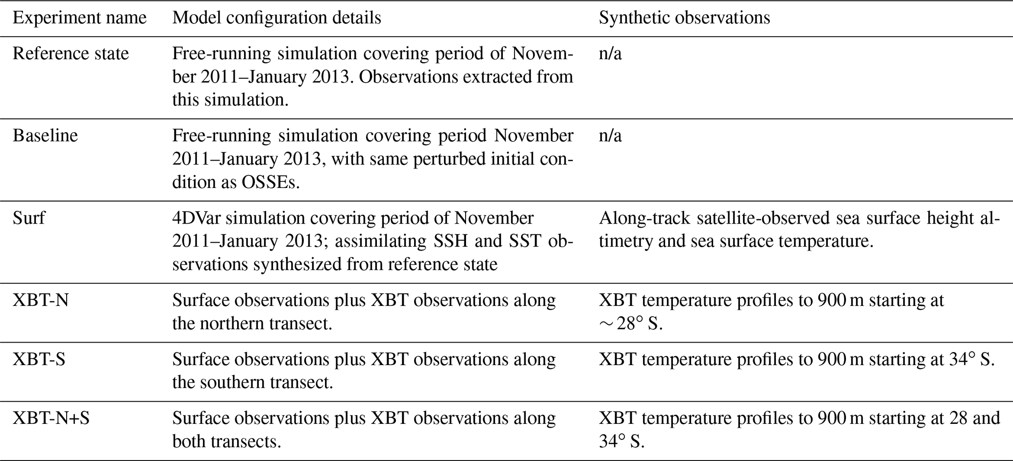
n/a: not applicable; indicates details not applicable for the forward-running reference state.
2.4 The OSSEs
OSSEs were conducted to evaluate observations from several observing platforms, both existing and hypothetical, to ascertain the impact on key dynamical features. Henceforth, “observation” refers to the synthetic observations which are derived from the free-running model. We conducted four different OSSEs as shown in Table 1. The “Surf OSSE” contains surface-only observations of SSH and SST, the “XBT-N OSSE” contains the same surface observations and the northern XBT transect, the “XBT-S OSSE” contains surface observations and the southern XBT transect, and the “XBT-N+S OSSE” contains surface observations with both northern and southern XBT transects.
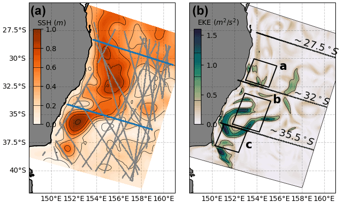
Figure 3Snapshots of model conditions with examples of observations and analysis regions. (a) A snapshot of SSH (colour map) is shown with a single 5 d cycle of SSH (grey dots) and XBT (blue dots) observations. (b) A snapshot of EKE (colour map) is shown, with boxes and lines showing key regions and diagnostic transects used in the analysis.
An example of SSH and XBT observation locations is shown in Fig. 3a. Realistic sampling patterns were used for satellite-observed SSH (e.g. all SSH observations in a 5 d DA cycle are shown in Fig. 3a), SST observations, and subsurface temperature from XBT lines that measure temperature to 900 m in the north and south of the domain (Fig. 3a). Details on all observation types are discussed below.
2.4.1 SSH
SSH observation timing and locations are taken from the global ocean along-track multi-mission sea level altimeter data (available at Copernicus Marine Service; https://doi.org/10.48670/moi-00146, CMEMS, 2022). This dataset has horizontal and along-track spacing and temporal repeats that vary between missions. For example, for the Jason-2 satellite, along-track sampling is ∼ 7 km. Observation locations are removed in water shallower than 1000 m and near to the model domain border (within 10 cells from the eastern and southern borders and within 60 cells from the northern border), so as to reduce mismatch between boundary forcing and assimilated observations. SSH observations at the timing and along-track locations are extracted from the reference state, and the track is replicated 2 h before and after each track, so as to inhibit the formation of barotropic waves through the 4DVar adjustment (for more details see Levin et al., 2021). During the processing of the raw data, we generate “super observations” by averaging multiple observations within a grid cell and within a 5 min window, to produce a single observation value which is then provided to the reference state simulation. A single cycle (5 d period) of SSH observations can lead to a relatively sparse SSH observation field (as per the example in Fig. 3a), especially in comparison to a daily gridded SSH observation field, e.g. from AVISO (Kerry et al., 2016). Each SSH along-track observation extracted from the reference state is perturbed such that the perturbations have normal distribution with a standard deviation equal to the applied observation error, which for along-track SSH is 0.04 m.
2.4.2 SST
SST observation timing and locations are chosen to represent data sourced from the gridded, near-real time Himawari-8 satellite product. The grid for these data is time-invariant and at a higher resolution (2 km) than the model grid. As a result, we choose each model point as an observation location, and have no need to superpose or thin observations. Further, and likewise for the other synthetic observation types, there are no representation errors, as we sample observations from the same model; realistic errors are added with random noise (see below). In order to reproduce realistic observation density, observations are masked by the realistic cloudiness field taken from the atmospheric reanalysis product used for surface forcing (Su et al., 2019). As there is no exact match between the BARRA-R cloudiness and the cloud matching algorithm used to process Himawari-8 data, we chose a simple cloudiness fraction (0.75) and discarded any observation locations with heavier cloud than this value. The choice of cloudiness fraction was calibrated by comparing the resulting fields against Himawari-8 images. Furthermore, we discarded any observations at times with wind speeds less than 2 m s−1 and during the day (to reduce mismatch between skin layer temperature and bulk SST, e.g. M. Yang et al., 2020). Lastly, SST data near the coastline (shallower than 100 m) or within 10 cells of the boundaries are removed to avoid contamination. Observation error is set at 0.5 ∘C and is added as a random perturbation to the observation values. Raw SST observations are processed in the same manner described above, where observations co-located within a cell or within a 5 min period are averaged to give a single value per cell. As the SST data are at a similar resolution to the model grid, an example field of observations is not shown in Fig. 3a.
2.4.3 XBT
XBT locations were generated to very approximately match XBT deployments along two of the Scripps high-resolution XBT program lines: PX30 from Brisbane to Nouméa and the PX34 line from Sydney to Wellington. These transects are occupied nominally quarterly, with a horizontal spacing of between approximately 10 to 100 km. In our case, synthetic temperature transects are cross-shore, parallel to the model grid, with casts every model cell. The resultant synthetic XBT transects (Fig. 3a; blue lines) are approximately perpendicular to the EAC at ∼ 28 and ∼35∘ S, and extend to within 10 cells of the domain boundary. Each temperature profile is extracted along the line with a time gap of 30 min, producing a full transect in approximately 5 d. The transect is then repeated from west to east again, with a 7 d duration between the beginning of each transect. Profiles extract synthetic observations from 5 to 900 m at the centre of each model cell (except where vertical resolution is finer than 10 m, in which case observations are limited to be at every 10 m to match the real XBT data). While the depth extent of our synthetic observations replicates the PX30 and PX34 lines, our spatial and temporal density is much higher (approximately weekly instead of quarterly). The observation error is added as a normally distributed random perturbation with a depth-dependent profile. This error profile was developed from a climatology of depth profiles in the EAC and should capture changes in temperature variance with depth (Kerry et al., 2016). The error profile has a subsurface maximum of 0.6 ∘C at 300 m then decreases to 0.12 ∘C at 1100 m. Like with SSH and SST, the XBT observation error is applied as a random normal perturbation to the synthetic observations.
2.5 Key dynamic metrics
We define several key metrics, which are chosen to test the improvement in the simulation of EAC dynamics, as ultimately this is the area of interest for improved prediction. We will assess quantities that are relevant for the key uncertainties highlighted in Sect. 1, namely, ocean heat content at different depths, spatial localization of the EAC jet, and the characteristics of the EAC eddy field.
2.5.1 Mean kinetic energy (MKE) and eddy kinetic energy (EKE)
MKE and EKE have been used previously for model validation of the EAC jet and the EAC eddy field (e.g. Li et al., 2021a). Here, we use EKE and MKE as metrics for assessing how well our OSSEs represent the EAC and EAC eddy field. For flow components in the zonal and meridional directions (u and v, respectively), we calculate MKE as half of the sum of the squared time-mean velocity components, as in . The EKE is then half of the sum of the squared-anomaly of the velocity components from the long-term mean, as in . The time-mean zonal () and meridional () components are averages of the instantaneous velocities over the full model integration (November 2011 to January 2013), as in u′ = , with v′ defined likewise. Note that all kinetic energies are given as values per unit mass. We explore these metrics at the surface and at 500 m, below the typical depth of the core of the EAC jet.

Figure 4The surface MKE for the (a) reference state, and OSSEs (b) surf, (c) XBT-N, (d) XBT-S, (E) XBT-N+S, and the MKE at 500 m for the (f) reference state, and OSSEs (b) surf, (c) XBT-N, (d) XBT-S, and (e) XBT-N+S. Black lines in panels (b)–(d) indicate location of the XBT lines. Key circulation features that emerge in the long-term mean are shown, including the EAC eastern and southern extensions and the return flow, which flow eastwards, southwards, and northwards, respectively.
2.5.2 Root mean square error
The root mean square error (RMSE) is calculated as , where the time mean (shown with an overbar) is taken of the difference between a reference field and the quantity in question X, at each grid point. Here we apply this standard definition to compute a temporally averaged RMSE, by taking the mean of the difference at every model output time separately for each model cell.
2.5.3 Upper ocean heat content (UOHC)
We calculate a volume-integrated upper ocean heat content (UOHC) by taking the depth and spatial integral of temperature, scaled by the specific heat capacity (cp = 3850 ) and reference density (ρ0 = 1026 kg m−3), as in
where the integrals extend from the surface to a specified depth (H), and over the region ξ1 to ξ2 in the model-space x direction and η1 to η2 in the model-space y-direction. The regions chosen are specified with model-space coordinates (rather than geographic coordinates) so that they are roughly aligned in the cross- and along-shelf directions.
The integrated UOHC is calculated for three regions. The first region (region a in Fig. 3b; centred at 154∘ E, 31.3∘ S) covers the EAC jet, upstream of the typical EAC separation zone. This region is chosen to capture heat in the EAC core, typically before it meanders and forms eddies. The second box (region b in Fig. 3b; centred at 153.5∘ E, 34.6∘ S) is aligned over the EAC eddy field and separation zone, in a region identified to have the highest surface magnitudes and variability in EKE as per (Li et al., 2021a). The third box (region c in Fig. 3b; centred at 151.5∘ E, 37∘ S) is located over the EAC southern extension (see Oke et al., 2019), in a region identified to have the highest rate of UOHC warming over the two decades from 1996–2016 (Li et al., 2022a), and so is an important region to represent correctly in models.
3.1 Spatial representation of the EAC
Key circulation features of the EAC, which emerge in the long-term average (Oke et al., 2019), include the EAC southern extension (which continues south following the shelf), the EAC return flow (which heads north on the eastward side of the EAC retroflection), and the EAC eastern extension (which flows eastwards towards New Zealand). All of these features are observed in the time-mean MKE of the Reference state (Fig. 4a at the surface and to a lesser extent at 500 m depth in Fig. 4f).

Figure 5The differences in spatial representation of temperature between the reference state and each OSSE. (a) The mean temperature field at 250 m in the reference state, with contours of standard deviation in that field. The rms error between the reference state and the OSSEs (b) surf, (c) XBT-N, (d) XBT-S, (e) XBT-N+S, and (f) the baseline simulation. The second row (panels g–l) is the same, but at 500 m, and the third row (panels m–r) shows the same fields at 1000 m. Note that colour scales are identical for all rms error plots. In reference state panels, contours are the standard deviation in the respective field while in all OSSE panels, the contours are of RMSE. Contour intervals are the same for all panels and are shown as a line in the RMSE colour bar. Black lines in panels (c–e) indicate location of the XBT lines. The area-mean RMSE and the mean RMSE over the high EKE region in box b (see Fig. 3b) are shown for each OSSE.
The surface-only OSSE (surf) has reduced energy through the EAC return flow region, that is, south of 34∘ S (Fig. 4b). Other features are fairly well represented. Both of the northern and southern XBT OSSEs represent the surface MKE of the reference state well, with a clear jet, separation region, return flow, and two bands of eastern extension (Fig. 4c and d). The XBT-N+S experiment has poor representation of the return flow, but, unlike the surface-only experiment, poorly captures the eastern extension (Fig. 4e).
In the reference state, at 500 m, the magnitude of MKE is substantially reduced but dominated by the jet region and the return flow (Fig. 4a and f). At this depth, there are more significant changes to the MKE distribution in the OSSEs, which all overestimate the magnitude of MKE at 500 m, a demonstration that reanalyses struggle to resolve conditions at depth. The surface-only observations do not constrain MKE well at 500 m depth, leading to anomalously deep re-circulation features throughout the domain (Fig. 4g). The addition of temperature observations along the northern transect (Fig. 4h) produces a better representation of the return flow, but re-circulation features form along the EAC (for example at 32.5∘ S), without feeding any eastward flow. The XBT-S experiment (XBT-S; Fig. 4i) best reproduces the reference state MKE pattern, with a clear return flow and eastern extension, though the magnitude of MKE at 500 m is too high (as in all the OSSEs). When both XBT transects are present (Fig. 4j), MKE is again poorly represented, with re-circulation too far north in the Tasman Sea (at 35∘ S).
The representation of the EAC eddy field, captured in EKE at the surface and 500 m is similarly represented in all OSSEs (see Fig. B1a–j).
3.2 Spatial representation of temperature
The surface temperature conditions are dominated by the extension of warmer water carried southwards by the EAC (Fig. 1). As all OSSEs assimilate the same SST data, the differences in representation of surface temperature are negligible (not shown). Instead, the spatial differences in representation of temperature fields below the surface are shown at 250, 500, and 1000 m in Fig. 5. For each field and OSSE, the area-mean rms value and the mean rms error for the high EKE region (box b; Fig. 3b) are shown in Fig. 5.
The error in temperature at 250 m is much higher for the surf OSSE (Fig. 5b), indicating that surface observations alone are not enough to constrain conditions at intermediate depths, and actually degrade temperature representation at 250 and 500 m (compared to the baseline; Fig. 5f and l), but by 1000 m depth, the error is lower (as it is for all OSSEs). The presence of the subsurface observations greatly improves 250 m temperature RMS (Fig. 5c–e; compare RMSE values in the eddy region of 1.6–1.8 to 2.5 ∘C for surf). Assimilating the southern XBT transect removes the band of high RMSE in the EAC eddy field at 34∘ S which is dominant in the surf OSSE and the northern XBT transect OSSE (cf. Fig. 5d to Fig. 5b and c). Note the improvement in rms error upstream of the XBT-S transect location, compared to surface-only observations. The addition of the north and south transects in the XBT-N+S OSSE (Fig. 5e) improves temperature rms compared to the surf OSSE, and has a similar spatial pattern in rms error to the southern XBT OSSE, with a mean RMSE of 1.7 ∘C in the eddy region, compared to 2.5 ∘C for the surf OSSE.
At 500 m, the error in temperature is generally slightly lower for each OSSE compared to the 250 m temperature field, though the reduced variability at depth likely partly accounts for this (compare contours of standard deviation in the temperature of reference state at 250, 500, and 1000 m; Fig. 5a, g and m). The OSSEs with either a northern or southern transect of XBT observations (Fig. 5i and j) display relatively low rms error, especially compared to the surface-only observations (Fig. 5h; area mean rms of 0.9 ∘C compared to 1.7 ∘C for surf). The addition of both transects together (Fig. 5k) slightly increases rms error in the separation zone.
Temperature at 1000 m is represented with similar rms error in all experiments (Fig. 5n–q). The lower temporal variability (Fig. 5m) in temperature at this depth likely leads to good representation from the boundary forcing conditions for all experiments.
Assimilation of SSH and SST observations ensures the correct spatial and temporal evolution of the eddy field at the surface, leading to all OSSEs performing better than the baseline (see Fig. B2). All of the OSSEs that include subsurface observations produce better representation of subsurface conditions at 250 and 500 m than the baseline simulation, particularly in the high eddy region (cf. Fig. 5c–e to Fig. 5f; Fig. 5i–k to Fig. 5l). The area mean RMS values for the baseline are marginally lower than XBT-S for temperature at 250 m and all OSSEs at 500 m, but when considering the mean over the eddy region, the baseline simulation has a higher mean RMS than the subsurface OSSEs. This is because the spatial and temporal evolution of the dynamic eddy field is better captured with data assimilation. Rms errors at 1000 m are slightly greater for all OSSEs than the errors in the perturbed run (cf. Fig. 5n–q and r). This is explained by the lower natural variability at this depth, which necessarily makes the free-running baseline more accurate through lower impact of that initial perturbation. Furthermore, the corrections that the 4DVar scheme makes often lead to a degradation in vertical representation. From hereon, we exclude comparison to the baseline so as to focus on the impact of the subsurface observations compared to the surface-only experiment.
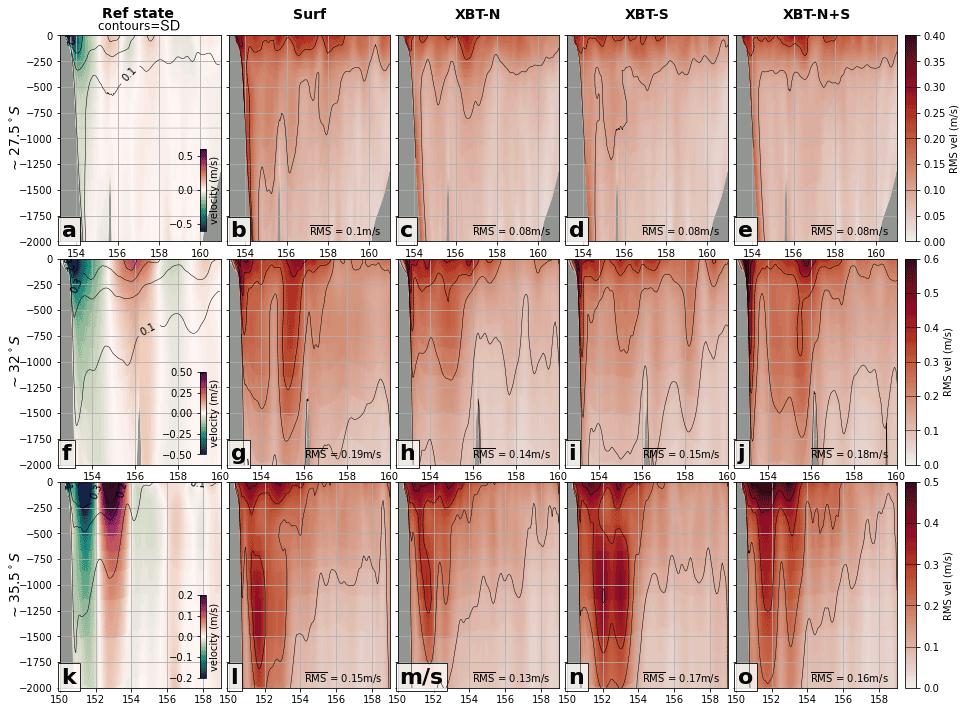
Figure 6Vertical cross-sections of meridional (north/south) velocity at key transects (first row) ∼ 27.5∘ S, (second row) ∼ 32∘ S, and (third row) ∼ 35.5∘ S are shown for each experiment. (a) The time-mean velocity (northwards–positive) in the reference state, with contours of standard deviation in the reference state velocity. The rms error between the reference state and the OSSEs (b) surf, (c) XBT-N, (d) XBT-S, and (e) XBT-N+ is shown at the transect ∼ 27.5∘ S. The second row (f–j) shows the same fields as the first row, but for the second transect at ∼ 32∘ S, while the third row (k–o) shows the same fields but for the third transect at ∼ 35.5∘ S. In reference state panels, contours are the standard deviation in the respective field while in all OSSE panels, the contours are of RMSE. Contour intervals are shown as a line in the RMSE colour bar. The depth-averaged RMSE of the region shown in each panel is included in the bottom corner.
3.3 Representation of velocity
Simulated northwards velocity (positive northwards) at key transects are best resolved with the addition of subsurface observations (Fig. 6). In the upstream region, the EAC core (strong southward flow above 250 m between the coast and 154∘ E; Fig. 6a) is a region of higher rms error in all OSSEs (Fig. 6b–e), but is improved with subsurface observations (e.g. compare Fig. 6b to Fig. 6c–e). Notably, the presence of the southern XBT line reduces rms velocity error in the EAC jet and on the slope (Fig. 6d) to levels comparable to the rms for the northern XBT line (Fig. 6c).
In the separation region, the mean southward EAC (from the coast to 155∘ E) and the northward return flow between 155–158∘ E (Fig. 6f) are regions of high rms error in the surface-only (Fig. 6g) OSSE. The southern XBT line OSSE (Fig. 6i) reduces this error within the southward EAC flow and return flow, particularly between 200–1500 m; notably, rms error below the deepest XBT observation (that is, deeper than ∼ 900 m) is also reduced compared to the surface-only experiment. When both transects are present (Fig. 6j), rms error on the shelf break and deeper than 1000 m increases compared to either OSSE with only a single observation transect.
In the downstream eddy-rich region, rms error is generally high in all OSSEs, as would be expected in this dynamic and less predictable region. The addition of temperature observations at depth does little to improve meridional velocity rms as compared to surface-only observations.

Figure 7Differences in vertical transects of temperature for each experiment are shown for the ∼ 27.5, ∼ 32, and ∼ 35.5∘ S transects. (a) The mean temperature of the reference state with contours of standard deviation. The rms error between the reference state and the OSSEs (b) surf, (c) XBT-N, (d) XBT-S, and (e) XBT-N+S is shown at the ∼ 27.5∘ S transect. The second row (f–j) shows the same fields as the first row, but for the second transect at ∼ 32∘ S, while the third row (k–o) shows the same fields but for the third transect at ∼ 35.5∘ S. In reference state panels, contours are the standard deviation in the respective field while in all OSSE panels, the contours are of RMSE. Contour intervals are shown as a line in the RMSE colour bar. The depth-averaged RMSE of the region shown in each panel is included in the bottom corner.
3.4 Representation of vertical temperature structure
The time-mean temperature at three cross-slope transects located upstream, near the separation zone and downstream in the high EKE region (see Fig. 3b for locations) is shown in Fig. 7. These transects are not co-located with the XBT lines. The reference state shows cooler temperatures further south and the isotherm deepening associated with warm core eddy downwelling (first column).
For the upstream transect (∼ 27.5∘ S; Fig. 7a), rms error in temperature is improved when depth observations are included, as compared to the surf OSSE (cf. Fig. 7c–e to b). The improvement in the representation of the EAC jet core temperature (i.e. temperature in the region between the coastline and 155∘ E, above ∼ 1000 m) is present for all OSSEs. While the lowest rms error along this transect is produced by the northern XBT transect OSSE (which is understandable given the proximity of the sampled transect and the observations), the southern transect OSSE also has far lower rms error than the surf OSSE, despite the southern XBT observations being ∼ 600 km distant. The mechanisms that might lead to such action at a distance are discussed further in Sect. 4.1 and 4.3.
Nearer to the separation zone (∼ 32∘ S; Fig. 7f), rms error for the surf OSSE is higher, especially in the mid depths of 250–500 m (Fig. 7g), with this region of higher error stretching down to 1000 m. The addition of subsurface observations in either the north or the south reduces rms error near the separation zone (Fig. 7h and i; depth averaged rms values of 0.7 ∘C, as compared to 1.0 ∘C for the surf OSSE), indicating an improvement in the representation of heat content carried by eddies.
In the eddy-rich region (∼ 35.5∘ S; Fig. 7k), the region of greatest rms error is again the 250–500 m depths at 152∘ E. Both single transect experiments retain a relatively high rms error, often extending to 1500 m. The XBT-N+S OSSE has good representation of temperature along this transect and much improved representation below 1000 m (Fig. 7o; depth-averaged rms of 0.6 ∘C); and indeed considering all transects (Fig. 7e, j and o), the XBT-N+S OSSE has low rms error, as opposed to the single XBT OSSEs, which have high rms at some transect locations (e.g. Fig. 7h and n).
3.5 Representation of upper ocean heat content
Volume-integrated upper ocean heat content, in three regions of interest and across the top 700 and 2000 m, is best simulated with the addition of subsurface observations (Fig. 8). The temporal evolution of UOHC for the reference state (Fig. 8; solid blue line shallower than 700 m and dashed blue line, shallower than 2000 m) is shown in comparison to each OSSE. The rms errors in UOHC between each OSSE and the reference state are shown in Table C1.

Figure 8The temporal evolution of integrated upper ocean heat content for three key regions: (a) upstream of the EAC separation zone, (b) the high EKE variability region, and (c) the region with strong UOHC trends, with locations shown in inset. The upper 700 m is shown with solid lines and the upper 2000 m is shown with dashed lines. Note the broken y axes.
In the region immediately upstream of the typical EAC separation zone (Fig. 8a; see box a in inset), all OSSEs represent UOHC content relatively poorly (Fig. 8a; reference state is blue line). For the upper 700 m, the XBT-N transect best represents UOHC (RMSE = 0.090 ZJ; Table C1), while for the upper 2000 m, the best representation of UOHC is in OSSEs that contain either the XBT-N or XBT-S transects (which both share RMSE = 0.13 ZJ; Table C1). It is noteworthy that the surf OSSE consistently gives the worst representation of UOHC in all three boxes (with RMSE ranging from 0.18–0.35 ZJ for the upper 700 m and RMSE ranging from 0.18–0.27 ZJ for the upper 2000 m; see Table C1).
This improved representation of UOHC in OSSEs with either XBT-N or XBT-S is again featured in the high EKE variability region (Fig. 8b; see box b in inset). Including the southern transect (XBT-S; Fig. 8b green line) gives the best representation shallower than 700 m (RMSE = 0.093 ZJ; Table C1), though this is somewhat expected given that XBT-S passes through this region. UOHC for the upper 2000 m is equally well represented by either XBT-N or XBT-S (RMSE = 0.083 ZJ; Table C1).
In the region of greatest upper UOHC trends (Fig. 8c; see box c in inset) as identified in Li et al. (2022a), we again see the best match between the reference state and the XBT-S OSSE, especially for the upper 2000 m (RMSE = 0.086 ZJ; Table C1). It is notable that the southern XBT transect improves UOHC upstream (in box a) and downstream (in box c) of its location, and down to depths of 2000 m, well below the deepest XBT observation.
The periods of increased or decreased error between the reference state and the OSSEs, and between each OSSEs, generally coincide with periods of more northerly or southerly EAC separation latitude (see Sects. 3.6 and 4.4). For example, during mid-January and May 2012, there was relatively good agreement in UOHC, which coincided with periods of southern EAC separation. Conversely, in October, when the EAC separated further north, most OSSEs had increased error compared to the reference state. Interestingly, while all OSSEs have generally worse representation of UOHC in the upstream box a region, there are periods of lower RMS, for example in early to mid-August, when there is a coherent EAC jet through the box a region, and likewise with box c in late April. This suggests that the ability to represent UOHC depends on the location of the coherent EAC jet and separation latitude.
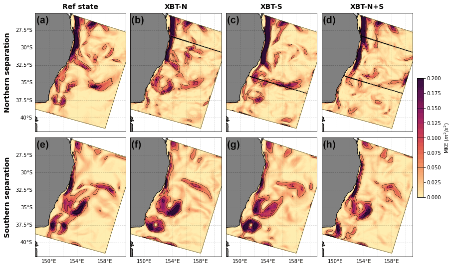
Figure 9The surface MKE is compared between the (a) reference state, (b) XBT-N, (c) XBT-S, and (d) XBT-N+S for the case when the EAC is in a northern separation phase. For the southern separating EAC phase, the surface MKE is compared between the (e) reference state and the (f) XBT-N, (g) XBT-S, and (h) XBT-N+S. Black lines in panels (b–d) indicate location of the XBT lines.
3.6 Observation impact during different EAC phases
When the EAC sheds large anticyclonic eddies, there is a rapid retraction of the EAC separation latitude. Typically, this EAC separation region is between 31 to 32∘ S (e.g. Cetina-Heredia et al., 2014); however, separation can occur north or south of this typical separation zone. As the presence of the EAC jet or large anticyclonic eddies will change meridional heat supply, downstream conditions will be different during northern or southern separation phases. Consequently, fixed location observations may have a different impact on representing the EAC and eddy field during different EAC phases. We have chosen two 2-month periods that represent “northern separation” (1 September 2012 to 1 November 2012) and “southern separation” (1 March 2012 to 1 May 2012) phases. Selected metrics are then compared between experiments within and between these northern and southern separation phases to illustrate the differences in observation impact.
For the period 1 September 2012 to 1 November 2012, the EAC separated further north than the mean, at ∼ 31.5∘ S (Fig. 9a) in the reference state. As we have established in Sect. 3 that including subsurface observations provides the best representation of EAC circulation and vertical structure, we exclude the surf OSSE and show only the OSSEs that include subsurface observations together with SSH and SST observations.
For this period, MKE is best represented in the experiments with either the northern or southern subsurface observation transect (cf. Fig. 9a and 9b and c). Only the XBT-N and XBT-S experiments have the separation and flow into the eastern extension at the correct location (with MKE connecting from the northern separation point to 156∘ E, 35∘ S) and with realistic magnitude. Adding both XBT transects produces separation further south and reduced MKE in the eastern extension (Fig. 9d).
Over the period 1 March 2012 to 1 May 2012, the EAC separated further south, with a separation at 35∘ S and re-attachment feeding the southern extension and initiation of the return flow at 38∘ S (Fig. 9e). When the EAC separates further south, there is a connected band of MKE along the coastline, re-circulation features at 35 and 38∘ S, a strong northward return flow, and an eastern flow extension. The magnitude of MKE in the jet is weaker than when the EAC separates further north. Both XBT experiments better represent these flow features along the coast and the northward return flow (Fig. 9f and g). The XBT-N+S OSSE does not represent the full extension of the EAC nor the return flow as well (Fig. 9h).
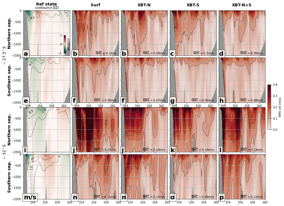
Figure 10The northwards velocity at ∼ 27.5∘ S is compared between the (a) reference state, (b) XBT-N, (c) XBT-S, and (d) XBT-N+S for the case when the EAC is in a northern separation phase, and for the (e) reference state, (f) XBT-N, (g) XBT-S, and (h) XBT-N+S in the southern separation phase. Likewise, the northward velocity is compared along the transect at ∼ 32∘ S for the (i) reference state, (j) XBT-N, (k) XBT-S, and (l) XBT-N+S OSSEs in the case when the EAC is in a northern separation phase. Lastly, velocities along the same transect in the (m) reference state, (n) XBT-N, (o) XBT-S, and (p) XBT-N+S OSSEs are compared for the southern separation phase. In the reference state panels, contours are the standard deviation in the respective field while in all OSSE panels, the contours are of RMSE. Contour intervals are shown as a line in the RMSE colour bar. The depth-averaged RMSE of the region shown in each panel is included in the bottom corner.
The northwards velocity during each separation phase and the error in representation displayed by each OSSE is shown in Fig. 10. During northern separation at ∼ 27.5∘ S, the jet region (Fig. 10a; upper 500 m west of 155∘ E) and surface ocean to a depth of 250 m are the sources of greatest error in the upstream region, for all OSSEs (Fig. 10b–d); however, observations in this upstream region (Fig. 10b and d; XBT-N and XBT-N+S) lead to the largest improvement in error in representation of the EAC jet, with depth-averaged RMS values of between 0.08–0.09 m s−1, as compared to 0.1 m s−1 for the surf and XBT-S OSSEs. During southward separation, the southern transect of subsurface observations produces the best representation of upstream velocity, including of the EAC jet (more so than northern XBT observations; cf. Fig. 10f and g).
During northern separation at ∼ 32∘ S (Fig. 10i), both experiments with a single subsurface XBT transect (XBT-N and XBT-S, Fig. 10j and k) have the lowest rms error (depth-averaged rms of 0.14 m s−1 compared to 0.19 m s−1 for XBT-N+S and 0.25 m s−1 for surf), but in general, velocity representation during a northern separation has the poorest representation, likely due to the dynamic features present in this region.
During southern separation, velocity representation along the ∼ 32∘ S transect is better in the presence of southern rather than northern subsurface observations (compare Fig. 10o to Fig. 10n; rms error of 0.08 m s−1 compared to 0.13 m s−1). This is another demonstration of the high observational impact of measurements taken in the eddy-rich region. The XBT-N+S OSSE has relatively high error in northwards velocity in this region (Fig. 10p), likely because the DA scheme is forced to minimize the error at both the north and south subsurface observations, resulting in a slightly degraded fit to either individually. Notably, at either the ∼ 32 or ∼ 27.5∘ S there is lower rms error in representation of velocity in all experiments, when the EAC separates further north (e.g. compare Fig. 10b–d and f–h).
4.1 Subsurface observations improve key EAC features
While the MKE of the EAC jet is well reproduced with surface-only observations, observations at depth are required to correctly represent other important EAC features. In particular, assimilating subsurface temperature (XBT) observations improves the representation of the northward return flow. The EAC eastern extension, which directs flow towards New Zealand (via an eddy train, see Oke et al., 2019), is best represented with the inclusions of temperature measurements through the southern section. Furthermore, only the experiment with subsurface temperature observations in the southern high EKE region reproduces these features at depth.
The better reproduction of key EAC features in the surface MKE fields (e.g. more energy in the southern extension, return flow, and eastern extensions; Fig. 4) when subsurface temperature observations (together with surface observations) are assimilated must be due to the improved subsurface conditions impacting the surface circulation. This highlights that correct density structure is important for resolving features such as the return flow and the EAC eastern extension, and geostrophic balance (i.e. conditions inferred from surface observations only) is not fully representative of flow in these features.
Other studies have also emphasized the importance of high-resolution and subsurface observations. In the Kuroshio Current, OSSEs showed that density changes resulting from subsurface temperature and salinity observations had a larger impact on WBC circulation than on deep, open ocean circulation (Lee et al., 2020). OSSEs conducted in the Gulf of Mexico found that higher spatial resolution subsurface temperature and salinity observations substantially reduced error by representing variability at scales too small to resolve by surface-only observations (Halliwell et al., 2015).
Surface EKE is not further improved with the assimilation of temperature observations at depth (see Fig. B1a–e). Furthermore, the improvement from temperature (XBT) observations on EKE at depth (500 m) is also minimal (Fig. B1g–j). While there is some improvement in EKE from the XBT-S transect, there was degradation in the far south of the domain. The limited impact is likely because EKE is a measure of the fast time-scale fluctuations in velocities, and temperature at depth has limited correlation with these rapid velocity changes. This is in contrast with MKE, as the mean flow is highly dependent on the subsurface temperature structure.
Observations of subsurface temperature at either XBT transect location vastly improve simulated temperature at 250–500 m compared to surface-only observations (although the southern XBT has more impact; see Sect. 3.4). This is consistent with Siripatana et al. (2020) who showed that the assimilation of subsurface observations (from a deep-water mooring array and ocean gliders) were required to correctly represent the depth of the EAC core and eddies. Improvement in the temperature field resulting from the subsurface observations also extends far upstream of the observation transect, indeed, “downstream” observations at 34∘ S improve representation northward, all the way to 27.5∘ S, over 600 km distant (Fig. 5d). This far-reaching impact was demonstrated in this 4DVar configuration of the EAC system by directly computing observation impact (Kerry et al., 2018); for example, temperature measurements from ocean gliders off 34∘ S were shown to impact estimates of EAC transport upstream at 27.5∘ N.
The vertical structure of eddies is complex, making them difficult to model. In this study, the greatest errors in representation are in the shallow–intermediate waters from 250–500 m (Fig. 7), particularly in the eddy-rich southern regions. Assimilating data along the northern XBT transect improves the vertical temperature structure in the upstream, shallow–intermediate waters, including in the EAC core (Fig. 7c), but does little to improve error in the temperature structure of more eddy-rich regions (cf. Fig. 7c and h and m). In contrast, including data from the southern XBT line improves representation of temperature both upstream and in the more eddy-rich regions of the typical EAC separation zone, and to a lesser extent, the southern Tasman Sea (Fig. 7d, i and n). While it is not surprising that temperature observations at depth improve the vertical temperature structure, it is notable that improvement extends to a depth of 1250 m, which is well below the deepest observation (900 m). Improvement below the depth of the observation transect also occurs for the meridional velocity. This suggests that conditions (temperature and velocities) at intermediate depths co-evolve with conditions above.
We have demonstrated that subsurface observations improve estimates of key quantities (e.g. temperature at depth), which is especially noticeable in the high EKE region. It has also been widely shown that the assimilation of subsurface observations has a strong impact on ocean state estimates (Moore et al., 2011a; Zavala-Garay et al., 2012). However, increasing the number of observations can lead to a reduced fit in any one single observation (e.g. compare the XBT-N+S RMS in Fig. 6j to RMS in XBT-S or XBT-N in Fig. 6h and i). This has also been demonstrated by others. For example, Siripatana et al. (2020) found that including extra data streams (HF radar currents and moorings) in addition to traditional observations (e.g. satellite SSH and SSH observations) degraded the model representation of SSH and SST. Zhang et al. (2010) showed that HF radar observations of currents degraded the subsurface temperature forecast, which they attributed to a lack of cross-variable covariance estimates.
4.2 Subsurface temperature observations improve UOHC representation
Given the improvement in representation of temperature and velocities at depth, due to the inclusion of two transects of subsurface temperature observations at relatively fine spacing, we would expect a marked improvement in the representation of UOHC. Indeed, we see that at all chosen locations, the inclusion of only surface observations in the surf OSSE leads to the poorest representation of UOHC compared to the reference state (Fig. 8), in contrast to when subsurface observations are included. This is true for both 0–700 and 0–2000 m integrated UOHC.
In particular, assimilating the XBT-S observations leads to the closest match with the reference state in the upper 700 m in the high variability region (Fig. 8b) and in the region identified in the southern Tasman Sea as having large UOHC trends (Fig. 8c). This southern XBT transect also improves UOHC both upstream (Fig. 8a) and downstream (Fig. 8c), indicating the far reaching impact of observations in this particular region.
Behrens et al. (2019) demonstrated a strong relationship between UOHC anomalies and the location, occurrence, and intensity of MHWs. In the southern Tasman Sea, a strong positive trend in EKE is also shown to be linked to a positive trend in UOHC (Li et al., 2022a). As a result, high-resolution subsurface temperature observations should improve representation of UOHC in model analyses, leading to improved predictability of MHWs. As MHWs can have significant ecological impacts, this strongly motivates the inclusion of subsurface observations in operational forecasts.
4.3 Downstream subsurface temperature observations are more impactful than upstream observations
For the many metrics that we have explored here, observations from the XBT-S transect were highly effective at assimilating towards the reference state, for example, MKE and EKE at 500 m and ocean heat content. This finding agrees with other literature which has suggested the importance of observing in high variability regions. Using an observational impact analysis, Kerry et al. (2018) found that observations in the region of high natural variability from 32S–37∘ S have the greatest impact per observation on transport estimates. In the Solomon Sea, Melet et al. (2012) suggested that gliders (which measure temperature and salinity) piloted through regions of high variability had a strong impact on reducing error in modelled thermocline properties.
The southern transect of subsurface observations improves the representation of conditions (e.g. horizontal and vertical temperature distribution) ∼ 600 km upstream (and in the region downstream of the separation zone and in the EAC eddy field). This is in contrast to the northern transect, which does not significantly improve conditions downstream of the separation zone. Possibly, this is because observing in a region where instabilities are beginning to grow constrains the conditions that led to eddy formation upstream, and is a tighter constraint on eddy evolution. For example, Li et al. (2021a) identify a band of strong barotropic energy conversion (mean flow shear-induced eddy generation) between 31.5 and 33.5∘ S, which is immediately north of the XBT-S observation transect.
In contrast, sampling upstream improves the EAC jet representation, but provides limited constraints on conditions after the EAC loses coherency and sheds eddies. This further illustrates that the depth structure of eddies is not well constrained by conditions in the upstream jet. Comparing the results of DA experiments including different observations, Siripatana et al. (2020) also showed that the constraint from an upstream, deep-water mooring array on the EAC core depth is effective where the jet is typically coherent, but degrades downstream in the eddy-dominated region.
4.4 Impact of EAC phase (separation latitude) on error in state estimates
The impact of surface-only and subsurface observations on the representation of EAC circulation features (e.g. eastern extension and return flow) and the vertical velocity structure differs depending on whether the EAC is separating to the north or south of the typical separation latitude range. The mean separation latitude ranges between 31–32∘ S (Cetina-Heredia et al., 2014; Oke et al., 2019); we identify northern separation as occurring between 28–31∘ S and southern separation occurring south of 32∘ S (results not shown). A separation to the north has been shown to be associated with a high energy EAC jet which becomes unstable and separates from the coast to the north of the typical separation latitude (Li et al., 2021a). This northern separation results in reduced heat transport to the south of the domain (as shown in Fig. 8, for example in October–September, by the reduced UOHC in box b and increased UOHC in box a). Conversely, a southern separation indicates a lower energy EAC jet, more stable mean flow upstream, and increased heat transport downstream. This is consistent with previous studies (Li et al., 2022a, 2021a) that showed a low frequency relationship between upstream EAC energy, separation latitude, and downstream UOHC. The results of Li et al. (2022a) were derived over interannual periods; we confirm this relationship for two specific 2-month periods in 2012.
When the EAC is separating to the north of the typical separation latitude range, representation of circulation, and vertical conditions (that is, the state estimate) have relatively high error. The error in UOHC between the OSSEs and the reference state is also related to separation latitude, as discussed above (Sect. 3.5). This is in contrast to a more southern separation, where the representation of these features is achieved with less error. For example, errors in estimates of the vertical structure of the EAC and eddy field are lower (compare rms error between Fig. 10b–d and f–h). Lower errors during southern separation are because the more stable EAC is less prone to instabilities which inhibit model skill.
During a northern separation phase, experiments with either line of subsurface observations (that is, XBT-N and XBT-S) produce similar representations of the EAC circulation and flow at depth (cf. Fig. 10b and c). Conversely, during southern separation, observations along the southern XBT line produce less error and a better estimate of the MKE and vertical structure of velocity (cf. Fig. 10f and g). The more accurate state estimates produced with downstream observations during a southern separation phase are another example of the impact of sampling in high variability regions. However, the reduced differentiation in model skill between XBT-N and XBT-S during a northern separation phase could result from several factors. The relative impact of either upstream or downstream observations may be balanced, because upstream observations are geographically closer to the separation region, while downstream observations are further south of the typical separation region. Together with the reduced coherency of the EAC making state estimates in general more difficult, this may act to equalize the impact of downstream or upstream observations on estimates of EAC conditions during a northern separation phase.
Observations and models suggest an intensification and southward migration of the extent of the EAC in recent decades (e.g. Cetina-Heredia et al., 2014; Hu et al., 2015), likely driven by a poleward shift of the South Pacific subtropical gyre H. Yang et al. (2020). Our two case studies show that a southward shift in the southern extension of the EAC, co-occurring with a weaker and more stable EAC system, should be able to be represented in DA models with lower error. Furthermore, if these long-term changes in the latitudinal extent of the EAC and EAC extension are as a result of more periods of lower MKE through the EAC jet, this could lead to more accurate simulation of downstream OHC and OHC extremes (such as marine heatwaves).
4.5 Implications for future observing system design
The experiments presented in this study are well suited for providing recommendations for future observing system design. As we show, subsurface temperature measurements improve the representation of the EAC structure including the return flow and eastern extensions, the spatial and vertical distribution of temperature within the ocean, vertical velocity shear and, therefore, ocean heat content. Kerry et al. (2018) also demonstrated the importance of subsurface observations, in particular, velocity and temperature observations at depth from deep mooring arrays and glider transects. The EAC transport array constrains velocities in the most coherent upstream EAC region, while gliders provide high spatial and temporal observation density in the eddy rich region that improve EAC transport and EKE. While we found that subsurface XBT observations were not significantly better at simulating EKE than just surface observations, we do see a difference below the surface. Our results suggest that subsurface temperature observations from XBT transects, given appropriate temporal and spatial density, and deployed in regions of high variability, can also improve representation of the EAC jet and other EAC features both up and downstream.
Observations in the region of high variability and high EKE, south of the typical EAC separation zone (e.g. XBT temperature transect at 35.5∘ S), are shown to disproportionately improve representation of the EAC, compared to just surface observations or to subsurface observations upstream. For this reason, observations taken in the high EKE region of the Tasman Sea will have a high cost-effectiveness in improving simulations of the EAC broadly. Along similar lines, O'Kane et al. (2011) speculate that observations targeting regions of large coherent forecast errors (e.g. the Tasman Sea) would improve subsequent forecasts.
Another interesting implication from this study is the varying impact of subsurface temperature observations during different dynamical regimes of the EAC; i.e. northern and southern separation phase. Hence, a sampling strategy that adapts to the changes in separation latitude can exploit the lower state estimate error during a low energy EAC phase. For example, during a high MKE, northern EAC separation phase, high density sampling could be used to capture MKE, vertical structure, and eddy shedding; this could be offset by reduced sampling in a low MKE, southern EAC separation phase.
These results suggest for future research that would further explore the subsurface representation of dynamic features and the cost-effectiveness of observing platforms in the EAC. For example, how does the simulated EAC jet and downstream features degrade as the (spatial and temporal) resolution of subsurface observations are degraded? Existing observing platforms of this style (high spatial resolution subsurface observations such as XBT transects) could also be assessed, and the spatial and temporal footprint of their impact could be measured.
The East Australian Current (EAC) is the western boundary current of the South Pacific subtropical gyre and dominates the oceanographic conditions in the Tasman Sea. Predictability of this current system is inhibited by the dynamic nature of the EAC eddy field. Using observing system simulation experiments, we explored how sea surface temperature and sea surface height observations in combination with subsurface temperature observations improve the representation of key EAC features in model state estimates. Improving model state estimates is key to improved prediction.
While assimilating surface observations is effective at improving representation of key EAC circulation features at the surface, such as the return flow and the southern and eastern extensions, surface observations struggle to represent these features at depth. In this study, we found that assimilating subsurface observations is critical for improving representation at depth. In particular, the northward return flow and eastern extension are represented only when including subsurface observations in the south of the domain. Not only is the vertical temperature structure improved with subsurface temperature observations, but so is the vertical velocity structure. As a result, upper ocean heat content, at key locations along the eastern seaboard, is best represented by assimilating subsurface temperature observations. Given the link between upper ocean heat content anomalies and marine heatwaves, improving representation of ocean heat content in simulations is a priority.
We demonstrate that observations taken in the high EKE region of the Tasman Sea have a strong impact on improving representation of the EAC and its vertical structure – upstream and downstream of the observing location. We posit that observing in the location where instabilities are growing into eddies gives information to the assimilation system of both the conditions that fed that instability and how the eddy will further evolve.
Importantly, we show that the energy of the EAC jet and the subsequent separation latitude has a strong impact on error in the representation of the EAC eddy field. A low MKE jet and southern separation will have lower representation error. This suggests that increased poleward transport of ocean heat, which is typically associated with a poleward separation latitude, should be easier to capture in models with fewer, more southerly observations.
Lastly, we suggest some sampling strategies for optimal reduction in error. For example, sampling in the high energy EAC eddy field will have a far-reaching improvement on the representation of the EAC. Likewise, sampling strategies could be designed to adapt dynamically to oceanographic conditions with higher resolution sampling upstream or downstream during northern EAC separation offset by lower resolution sampling in the downstream region during southern separation. Together with suggested sampling strategies, the links we show between subsurface observations, ocean heat content, and EAC dynamics should help to improve predictability of the EAC and associated eddy field.
In Fig. A1a and b, the spatial mean EKE and volume transport of the reference state are compared against the mean values of these same quantities derived from the free-running 1994–2016 simulation (e.g. Li et al., 2021a). Southward volume transport (which we calculate here as southward flow above 2000 m and west of 155∘ E, along a transect at ∼ 28∘ S) varies between 0 and 61 Sv (with a mean of 18 ± 15 Sv southwards), which compares favourably to the long-term (1994–2016) mean and standard deviation in volume transport of 21 ± 14 Sv. The time series of volume transport is also shown to generally fall within the bounds of 2 standard deviations of the long-term volume transport (Fig. A1b).
The time-mean EKE over the whole domain of the reference state (0.12 ± 0.027 m2 s−2) is very close to the long-term mean and standard deviation in EKE of 0.12 ± 0.028 m2 s−2. Likewise, except for several periods of rapid fluctuations, the EKE of the reference state also generally falls within 2 standard deviations of the long-term simulation (Fig. A1b).
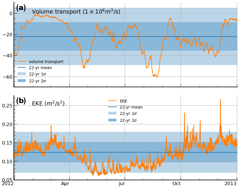
Figure A1Volume transport and EKE conditions of the 1-year free-running simulation. (a) Integrated volume transport through a transect at ∼ 28∘ S (orange line). The blue line is the mean volume transport from the 1994–2016 long-running simulation, while the darker and lighter shaded regions show ± 1 and ± 2 standard deviations. Likewise, (b) shows the spatial-mean EKE over the whole domain (orange line). The blue line and shaded regions showing the mean, ± 1, and ± 2 standard deviations, respectively, in EKE for the long-running 1994–2016 simulation.
The EAC eddy field is clearly visible in the mean EKE for the reference state (Fig. B1a). All OSSEs exhibit similar error in representation of this feature (Fig. B1b–e), with similar magnitudes of error to the error (standard deviation) in the EKE of the reference state (compare high RMS in Fig. B1b–e to contours in Fig. B1a). At 500 m depth, the EKE field is weaker, though it shares the same spatial footprint as at the surface (Fig. B1f). All OSSEs perform similarly, though the inclusion of the southern XBT transect (either by itself or together with the northern transect) produces the lower rms error (Fig. B1i and j).
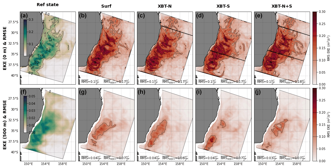
Figure B1The differences in spatial representation of EKE between the reference state and each OSSE. (a) The time-mean surface EKE of the Reference state, with contours of standard deviation in that field. The rms error between the reference state and the OSSEs (b) surf, (c) XBT-N, (d) XBT-S, and (e) XBT-N+S. The second row (panels f–j) shows the same fields for the EKE at 500 m. Note the identical colour scales for all rms error plots. In reference state panels, contours are the standard deviation in the respective field, while in all OSSE panels, the contours are of rms error. Contour intervals are the same for all panels and are shown as a line in the rms error colour bar. Black lines in panels (c–e) indicate location of the XBT lines.
The mean SSH in the reference state shows SSH maxima along the east coast (Fig. B2a). rms error in SSH is relatively similar between each OSSE. All of the OSSEs assimilate the same SSH observations, so the similarities indicate that the subsurface observations have little impact on the representation of SSH (Fig. B2b–e). The region of peak rms error matches the region of high variability in SSH (compare high rms in Fig. B2b–e to contours in Fig. B2a). The baseline simulation displays considerable more error in SSH (Fig. B2f). Like the SSH, the mean SST is similarly represented in all OSSEs, at a level of error similar to the rms in SST (cf. Fig. B2h–k and contours in Fig. B2g). SST representation in the baseline has considerable higher error than any OSSE (Fig. B2l).
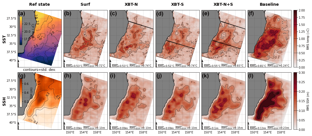
Figure B2The differences in spatial representation of SSH and SST between the reference state, each OSSE, and the baseline simulation. (a) The mean SSH of the reference state, with contours of standard deviation in that field. The rms error between the reference state and the OSSEs (b) surf, (c) XBT-N, (d) XBT-S, (e) XBT-N+S, and (f) baseline. The second row (panels (f–j)) shows the same diagnostics for the SST. In reference state panels, contours are the standard deviation in the respective field, while in all OSSE panels, the contours are of rms error. Contour intervals are the same for all panels and are shown as a line in the rms error colour bar. Black lines in panels (c)–(e) indicate location of the XBT lines. The area-mean RMSE and the mean RMSE over the high EKE region in box b (see Fig. 3b) are shown for each OSSE.
The root mean square error (RMSE) in UOHC is calculated between the reference state and each OSSE (Table C1). The RMSE values are calculated for both UOHC calculations: the upper 700 and the upper 2000 m, and for all three regions of interest, which are designated in Fig. 3.
Table C1Root mean square error (RMSE) in upper ocean heat content (UOHC) for regions a, b, c (see Fig. 3b), over the top 700 m and top 2000 m. The RMSE value is shown for each experiment, compared to the reference state.

The exact version of the model, configuration files, and forcing files used to produce the results used in this paper are archived on Zenodo (https://doi.org/10.5281/zenodo.6804480, Gwyther et al., 2022a) and the UNSW library (https://doi.org/10.26190/unsworks/24146, Gwyther et al., 2022b).
DEG, CK, MR, and SRK conceived and designed the experiments. DEG and CK performed the simulations. DEG analysed the data. All authors contributed to interpretation of the results. DEG prepared the paper with contributions from all co-authors.
The contact author has declared that none of the authors has any competing interests.
Publisher's note: Copernicus Publications remains neutral with regard to jurisdictional claims in published maps and institutional affiliations.
Former model development was supported by Australian Research Council grants DP140102337 and LP160100162 to Moninya Roughan. This research was undertaken with the assistance of resources and services from the National Computational Infrastructure (NCI), under the grant fu5, and computations using the computational cluster Katana (https://doi.org/10.26190/669x-a286, Research Technology Services, UNSW Sydney, 2022) supported by Research Technology Services at UNSW Sydney. The authors thank Michael Dinniman, Helen Beggs, Pallavi Govekar, and two anonymous reviewers for their input. The current version of ROMS is available from the project website: https://www.myroms.org/projects/git-src/ (last access: 2 February 2021) under an open-source licence. We acknowledge that the forcing conditions are sourced from the Commonwealth Science and Industrial Research Organisation (BRAN2020; available at https://research.csiro.au/bluelink/outputs/data-access/, last access: 15 April 2021) and the Bureau of Meteorology (BARRA-R and ACCESS; http://www.bom.gov.au/research/projects/, last access: 2 February 2021). Along-track SSH data are sourced from the E.U. Copernicus Marine Service Information (https://doi.org/10.48670/moi-00146, CMEMS, 2022), and model configurations for the free-running and DA simulations are identical to those used in previous simulations (available online at https://doi.org/10.26190/TT1Q-NP46, Li et al., 2021b; https://doi.org/10.26190/5ebe1f389dd87, Kerry et al., 2020b).
This research and David E. Gwyther were supported by Australian Research Council Industry Linkage Grant LP170100498 to Moninya Roughan, Shane R. Keating, and Colette Kerry.
This paper was edited by Riccardo Farneti and reviewed by two anonymous referees.
Ballabrera-Poy, J., Hackert, E., Murtugudde, R., and Busalacchi, A. J.: An Observing System Simulation Experiment for an Optimal Moored Instrument Array in the Tropical Indian Ocean, J. Climate, 20, 3284–3299, https://doi.org/10.1175/jcli4149.1, 2007. a
Behrens, E., Fernandez, D., and Sutton, P.: Meridional Oceanic Heat Transport Influences Marine Heatwaves in the Tasman Sea on Interannual to Decadal Timescales, Frontiers in Marine Science, 6, https://doi.org/10.3389/fmars.2019.00228, 2019. a
Brink, K.: Cross-Shelf Exchange, Annu. Rev. Mar. Sci., 8, 59–78, https://doi.org/10.1146/annurev-marine-010814-015717, 2016. a
Cetina-Heredia, P., Roughan, M., van Sebille, E., and Coleman, M. A.: Long-term trends in the East Australian Current separation latitude and eddy driven transport, J. Geophys. Res.-Oceans, 119, 4351–4366, https://doi.org/10.1002/2014jc010071, 2014. a, b, c, d
Chamberlain, M. A., Oke, P. R., Fiedler, R. A. S., Beggs, H. M., Brassington, G. B., and Divakaran, P.: Next generation of Bluelink ocean reanalysis with multiscale data assimilation: BRAN2020, Earth Syst. Sci. Data, 13, 5663–5688, https://doi.org/10.5194/essd-13-5663-2021, 2021. a
Copernicus Marine Service (CMEMS): Global ocean along-track L3 sea surface heights reprocessed (1993-ongoing) tailored for data assimilation (SEALEVEL_GLO_PHY_L3_MY_008_062), Copernicus Marine Service (CMEMS) [data set], https://doi.org/10.48670/moi-00146, 2022. a, b
Elzahaby, Y. and Schaeffer, A.: Observational Insight Into the Subsurface Anomalies of Marine Heatwaves, Frontiers in Marine Science, 6, https://doi.org/10.3389/fmars.2019.00745, 2019. a
Elzahaby, Y., Schaeffer, A., Roughan, M., and Delaux, S.: Oceanic Circulation Drives the Deepest and Longest Marine Heatwaves in the East Australian Current System, Geophys. Res. Lett., 48, e2021GL094785, https://doi.org/10.1029/2021gl094785, 2021. a
Fairall, C. W., Bradley, E. F., Rogers, D. P., Edson, J. B., and Young, G. S.: Bulk parameterization of air–sea fluxes for Tropical Ocean–Global Atmosphere Coupled–Ocean Atmosphere Response Experiment, J. Geophys. Res.-Oceans, 101, 3747–3764, https://doi.org/10.1029/95jc03205, 1996. a
Gasparin, F., Guinehut, S., Mao, C., Mirouze, I., Rémy, E., King, R. R., Hamon, M., Reid, R., Storto, A., Traon, P.-Y. L., Martin, M. J., and Masina, S.: Requirements for an Integrated in situ Atlantic Ocean Observing System From Coordinated Observing System Simulation Experiments, Frontiers in Marine Science, 6, https://doi.org/10.3389/fmars.2019.00083, 2019. a
Gwyther, D. E., Kerry, C., Roughan, M., and Keating, S.: A high-resolution, 1-year, suite of 4D-Var Observing System Simulation Experiments of the East Australian Current System using the Regional Ocean Modeling System (1.0), Zenodo [code and data set], https://doi.org/10.5281/zenodo.6804480, 2022a. a
Gwyther, D. E., Kerry, C., Roughan, M., and Keating, S.: A high-resolution, 1-year, suite of 4D-Var Observing System Simulation Experiments of the East Australian Current System using the Regional Ocean Modeling System, UNSW Sydney [code and data set], https://doi.org/10.26190/unsworks/24146, 2022b. a
Halliwell, G. R., Srinivasan, A., Kourafalou, V., Yang, H., Willey, D., Hénaff, M. L., and Atlas, R.: Rigorous Evaluation of a Fraternal Twin Ocean OSSE System for the Open Gulf of Mexico, J. Atmos. Ocean. Tech., 31, 105–130, https://doi.org/10.1175/jtech-d-13-00011.1, 2014. a, b
Halliwell, G. R., Kourafalou, V., Hénaff, M. L., Shay, L. K., and Atlas, R.: OSSE impact analysis of airborne ocean surveys for improving upper-ocean dynamical and thermodynamical forecasts in the Gulf of Mexico, Prog. Oceanogr., 130, 32–46, https://doi.org/10.1016/j.pocean.2014.09.004, 2015. a, b
Halliwell, G. R., Mehari, M. F., Hénaff, M. L., Kourafalou, V. H., Androulidakis, I. S., Kang, H. S., and Atlas, R.: North Atlantic Ocean OSSE system: Evaluation of operational ocean observing system components and supplemental seasonal observations for potentially improving tropical cyclone prediction in coupled systems, J. Oper. Oceanogr., 10, 154–175, https://doi.org/10.1080/1755876x.2017.1322770, 2017. a
He, Z., Yang, D., Wang, Y., and Yin, B.: Impact of 4D-Var data assimilation on modelling of the East China Sea dynamics, Ocean Modell., 176, 102044, https://doi.org/10.1016/j.ocemod.2022.102044, 2022. a
Hu, D., Wu, L., Cai, W., Gupta, A. S., Ganachaud, A., Qiu, B., Gordon, A. L., Lin, X., Chen, Z., Hu, S., Wang, G., Wang, Q., Sprintall, J., Qu, T., Kashino, Y., Wang, F., and Kessler, W. S.: Pacific western boundary currents and their roles in climate, Nature, 522, 299–308, https://doi.org/10.1038/nature14504, 2015. a
Kamenkovich, I., Haza, A., Gray, A. R., Dufour, C. O., and Garraffo, Z.: Observing System Simulation Experiments for an array of autonomous biogeochemical profiling floats in the Southern Ocean, J. Geophys. Res.-Oceans, 122, 7595–7611, https://doi.org/10.1002/2017jc012819, 2017. a
Kawabe, M.: Variations of Current Path, Velocity, and Volume Transport of the Kuroshio in Relation with the Large Meander, J, Phys. Oceanogr., 25, 3103–3117, https://doi.org/10.1175/1520-0485(1995)025<3103:vocpva>2.0.co;2, 1995. a
Kerry, C. and Roughan, M.: Downstream Evolution of the East Australian Current System: Mean Flow, Seasonal, and Intra-annual Variability, J. Geophys. Res.-Oceans, 125, e2019JC015227, https://doi.org/10.1029/2019jc015227, 2020. a, b, c
Kerry, C., Powell, B., Roughan, M., and Oke, P.: Development and evaluation of a high-resolution reanalysis of the East Australian Current region using the Regional Ocean Modelling System (ROMS 3.4) and Incremental Strong-Constraint 4-Dimensional Variational (IS4D-Var) data assimilation, Geosci. Model Dev., 9, 3779–3801, https://doi.org/10.5194/gmd-9-3779-2016, 2016. a, b, c, d, e, f, g, h
Kerry, C., Roughan, M., and Powell, B.: Observation Impact in a Regional Reanalysis of the East Australian Current System, J. Geophys. Res.-Oceans, 123, 7511–7528, https://doi.org/10.1029/2017jc013685, 2018. a, b, c, d, e, f
Kerry, C., Roughan, M., and Powell, B.: Predicting the submesoscale circulation inshore of the East Australian Current, J. Marine Syst., 204, 103286, https://doi.org/10.1016/j.jmarsys.2019.103286, 2020a. a
Kerry, C., Roughan, M., Powell, B., and Oke, P: A high-resolution reanalysis of the East Australian Current System assimilating an unprecedented observational data set using 4D-Var data assimilation over a two-year period (2012–2013). Version 2017, UNSW Sydney [code and data set], https://doi.org/10.26190/5ebe1f389dd87, 2020b. a
Lee, J.-H., Chang, Y.-S., and Zhang, S.: Assessment of the JMA Serial Observation Lines in the Northwestern Pacific in OSSE Studies with the GFDL Ensemble Coupled Data Assimilation System, J. Geophys. Res.-Oceans, 125, e2019JC015686, https://doi.org/10.1029/2019jc015686, 2020. a, b
Levin, J., Arango, H. G., Laughlin, B., Wilkin, J., and Moore, A. M.: The impact of remote sensing observations on cross-shelf transport estimates from 4D-Var analyses of the Mid-Atlantic Bight, Adv. Space Res., 68, 553–570, https://doi.org/10.1016/j.asr.2019.09.012, 2021. a, b
Li, B., de Queiroz, A. R., DeCarolis, J. F., Bane, J., He, R., Keeler, A. G., and Neary, V. S.: The economics of electricity generation from Gulf Stream currents, Energy, 134, 649–658, https://doi.org/10.1016/j.energy.2017.06.048, 2017. a
Li, J., Roughan, M., and Kerry, C.: Dynamics of Interannual Eddy Kinetic Energy Modulations in a Western Boundary Current, Geophys. Res. Lett., 48, e2021GL094115, https://doi.org/10.1029/2021gl094115, 2021a. a, b, c, d, e, f, g, h, i, j, k, l, m
Li, J., Kerry, C., and Roughan, M.: A high-resolution, 22-year, free-running, hydrodynamic simulation of the East Australia Current System using the Regional Ocean Modeling System (Version 2.0), UNSW Sydney [code and data set], https://doi.org/10.26190/TT1Q-NP46, 2021b. a
Li, J., Roughan, M., and Kerry, C.: Variability and Drivers of Ocean Temperature Extremes in a Warming Western Boundary Current, J. Climate, 35, 1097–1111, https://doi.org/10.1175/JCLI-D-21-0622.1, 2022a. a, b, c, d, e, f, g, h, i
Li, J., Roughan, M., Kerry, C., and Rao, S.: Impact of Mesoscale Circulation on the Structure of River Plumes During Large Rainfall Events Inshore of the East Australian Current, Frontiers in Marine Science, 9, https://doi.org/10.3389/fmars.2022.815348, 2022b. a
Malan, N., Roughan, M., and Kerry, C.: The Rate of Coastal Temperature Rise Adjacent to a Warming Western Boundary Current is Nonuniform with Latitude, Geophys. Res. Lett., 48, e2020GL090751, https://doi.org/10.1029/2020gl090751, 2021. a, b
Melet, A., Verron, J., and Brankart, J.-M.: Potential outcomes of glider data assimilation in the Solomon Sea: Control of the water mass properties and parameter estimation, J. Marine Syst., 94, 232–246, https://doi.org/10.1016/j.jmarsys.2011.12.003, 2012. a, b
Moore, A. M., Arango, H. G., Broquet, G., Edwards, C., Veneziani, M., Powell, B., Foley, D., Doyle, J. D., Costa, D., and Robinson, P.: The Regional Ocean Modeling System (ROMS) 4-dimensional variational data assimilation systems: Part III – Observation impact and observation sensitivity in the California Current System, Prog. Oceanogr., 91, 74–94, https://doi.org/10.1016/j.pocean.2011.05.005, 2011a. a
Moore, A. M., Arango, H. G., Broquet, G., Powell, B. S., Weaver, A. T., and Zavala-Garay, J.: The Regional Ocean Modeling System (ROMS) 4-dimensional variational data assimilation systems: Part I – System overview and formulation, Prog. Oceanogr., 91, 34–49, https://doi.org/10.1016/j.pocean.2011.05.004, 2011b. a
Moore, A. M., Edwards, C. A., Fiechter, J., Drake, P., Neveu, E., Arango, H. G., Gürol, S., and Weaver, A. T.: A 4D-Var Analysis System for the California Current: A Prototype for an Operational Regional Ocean Data Assimilation System, in: Data Assimilation for Atmospheric, Oceanic and Hydrologic Applications (Vol. II), edited by: Park, S. K. and Xu, L., chap. 14, pp. 345–366, Springer Berlin Heidelberg, Berlin, Heidelberg, https://doi.org/10.1007/978-3-642-35088-7_14, 2013. a
Moore, A. M., Martin, M. J., Akella, S., Arango, H. G., Balmaseda, M., Bertino, L., Ciavatta, S., Cornuelle, B., Cummings, J., Frolov, S., Lermusiaux, P., Oddo, P., Oke, P. R., Storto, A., Teruzzi, A., Vidard, A., and Weaver, A. T.: Synthesis of Ocean Observations Using Data Assimilation for Operational, Real-Time and Reanalysis Systems: A More Complete Picture of the State of the Ocean, Frontiers in Marine Science, 6, https://doi.org/10.3389/fmars.2019.00090, 2019. a
Moore, A. M., Zavala-Garay, J., Arango, H. G., Edwards, C. A., Anderson, J., and Hoar, T.: Regional and basin scale applications of ensemble adjustment Kalman filter and 4D-Var ocean data assimilation systems, Prog. Oceanogr., 189, 102450, https://doi.org/10.1016/j.pocean.2020.102450, 2020. a
O'Kane, T. J., Oke, P. R., and Sandery, P. A.: Predicting the East Australian Current, Ocean Modell., 38, 251–266, https://doi.org/10.1016/j.ocemod.2011.04.003, 2011. a
Oke, P. R. and Schiller, A.: A Model-Based Assessment and Design of a Tropical Indian Ocean Mooring Array, J. Climate, 20, 3269–3283, https://doi.org/10.1175/jcli4170.1, 2007. a
Oke, P. R., Roughan, M., Cetina-Heredia, P., Pilo, G. S., Ridgway, K. R., Rykova, T., Archer, M. R., Coleman, R. C., Kerry, C. G., Rocha, C., Schaeffer, A., and Vitarelli, E.: Revisiting the circulation of the East Australian Current: Its path, separation, and eddy field, Prog. Oceanogr., 176, 102139, https://doi.org/10.1016/j.pocean.2019.102139, 2019. a, b, c, d
Oliver, E. C. J., Donat, M. G., Burrows, M. T., Moore, P. J., Smale, D. A., Alexander, L. V., Benthuysen, J. A., Feng, M., Gupta, A. S., Hobday, A. J., Holbrook, N. J., Perkins-Kirkpatrick, S. E., Scannell, H. A., Straub, S. C., and Wernberg, T.: Longer and more frequent marine heatwaves over the past century, Nat. Commun., 9, 1324, https://doi.org/10.1038/s41467-018-03732-9, 2018. a
Puri, K., Dietachmayer, G., Steinle, P., Dix, M., Rikus, L., Logan, L., Naughton, M., Tingwell, C., Xiao, Y., Barras, V., Bermous, I. Bowen, R., Deschamps, L., Franklin, C., Fraser, J., Glowacki, T., Harris, B., Lee, J., Le, T., Roff, G., Sulaiman, A., Sims, H., Sun, X., Sun, Z., Zhu, H., Chattopadhyay, M., Engel, C.: Implementation of the initial ACCESS numerical weather prediction system, Aust. Meteorol. Ocean., 63, 265–284, 2013. a
Research Technology Services, UNSW Sydney: Katana computational cluster, https://doi.org/10.26190/669x-a286, 2022. a
Ribbat, N., Roughan, M., Powell, B., Rao, S., and Kerry, C. G.: Transport variability over the Hawkesbury Shelf (31.5–34.5∘ S) driven by the East Australian Current, PLOS ONE, 15, e0241622, https://doi.org/10.1371/journal.pone.0241622, 2020. a
Richardson, P. L. and Knauss, J. A.: Gulf stream and Western boundary undercurrent observations at Cape Hatteras, Deep Sea Research and Oceanographic Abstracts, 18, 1089–1109, https://doi.org/10.1016/0011-7471(71)90095-7, 1971. a
Roughan, M., Schaeffer, A., and Suthers, I. M.: Sustained Ocean Observing along the Coast of Southeastern Australia: NSW-IMOS 2007–2014, in: Coastal Ocean Observing Systems, edited by: Liu, Y., Kerkering, H., and Weisberg, R. H., Elsevier, Boston, 76–98, ISBN 978-0-12-802022-7, https://doi.org/10.1016/b978-0-12-802022-7.00006-7, 2015. a
Roughan, M., Cetina-Heredia, P., Ribbat, N., and Suthers, I. M.: Shelf Transport Pathways Adjacent to the East Australian Current Reveal Sources of Productivity for Coastal Reefs, Frontiers in Marine Science, 8, https://doi.org/10.3389/fmars.2021.789687, 2022. a
Schiller, A., Wijffels, S. E., and Meyers, G. A.: Design Requirements for an Argo Float Array in the Indian Ocean Inferred from Observing System Simulation Experiments, J. Atmos. Ocean. Tech., 21, 1598–1620, https://doi.org/10.1175/1520-0426(2004)021<1598:drfaaf>2.0.co;2, 2004. a
Siripatana, A., Kerry, C., Roughan, M., Souza, J. M. A. C., and Keating, S.: Assessing the Impact of Nontraditional Ocean Observations for Prediction of the East Australian Current, J. Geophys. Res.-Oceans, 125, e2020JC016580, https://doi.org/10.1029/2020jc016580, 2020. a, b, c, d
Su, C.-H., Eizenberg, N., Steinle, P., Jakob, D., Fox-Hughes, P., White, C. J., Rennie, S., Franklin, C., Dharssi, I., and Zhu, H.: BARRA v1.0: the Bureau of Meteorology Atmospheric high-resolution Regional Reanalysis for Australia, Geosci. Model Dev., 12, 2049–2068, https://doi.org/10.5194/gmd-12-2049-2019, 2019. a, b
Todd, R. E., Chavez, F. P., Clayton, S., Cravatte, S., Goes, M., Graco, M., Lin, X., Sprintall, J., Zilberman, N. V., Archer, M., Arístegui, J., Balmaseda, M., Bane, J. M., Baringer, M. O., Barth, J. A., Beal, L. M., Brandt, P., Calil, P. H. R., Campos, E., Centurioni, L. R., Chidichimo, M. P., Cirano, M., Cronin, M. F., Curchitser, E. N., Davis, R. E., Dengler, M., deYoung, B., Dong, S., Escribano, R., Fassbender, A. J., Fawcett, S. E., Feng, M., Goni, G. J., Gray, A. R., Gutiérrez, D., Hebert, D., Hummels, R., ichi Ito, S., Krug, M., Lacan, F., Laurindo, L., Lazar, A., Lee, C. M., Lengaigne, M., Levine, N. M., Middleton, J., Montes, I., Muglia, M., Nagai, T., Palevsky, H. I., Palter, J. B., Phillips, H. E., Piola, A., Plueddemann, A. J., Qiu, B., Rodrigues, R. R., Roughan, M., Rudnick, D. L., Rykaczewski, R. R., Saraceno, M., Seim, H., Gupta, A. S., Shannon, L., Sloyan, B. M., Sutton, A. J., Thompson, L., van der Plas, A. K., Volkov, D., Wilkin, J., Zhang, D., and Zhang, L.: Global Perspectives on Observing Ocean Boundary Current Systems, Frontiers in Marine Science, 6, https://doi.org/10.3389/fmars.2019.00423, 2019. a
Whiteway, T.: Australian bathymetry and topography grid, June 2009, Record 2009/021, Geoscience Australia, Canberra, Australia, Department of Industry [data set], https://doi.org/10.4225/25/53D99B6581B9A, 2009. a
Wu, L., Cai, W., Zhang, L., Nakamura, H., Timmermann, A., Joyce, T., McPhaden, M. J., Alexander, M., Qiu, B., Visbeck, M., Chang, P., and Giese, B.: Enhanced warming over the global subtropical western boundary currents, Nat. Clim. Change, 2, 161–166, https://doi.org/10.1038/nclimate1353, 2012. a
Yang, H., Lohmann, G., Krebs-Kanzow, U., Ionita, M., Shi, X., Sidorenko, D., Gong, X., Chen, X., and Gowan, E. J.: Poleward Shift of the Major Ocean Gyres Detected in a Warming Climate, Geophys. Res. Lett., 47, e2019GL085868, https://doi.org/10.1029/2019gl085868, 2020. a
Yang, M., Guan, L., Beggs, H., Morgan, N., Kurihara, Y., and Kachi, M.: Comparison of Himawari-8 AHI SST with Shipboard Skin SST Measurements in the Australian Region, Remote Sensing, 12, 1237, https://doi.org/10.3390/rs12081237, 2020. a
Zavala-Garay, J., Wilkin, J. L., and Arango, H. G.: Predictability of Mesoscale Variability in the East Australian Current Given Strong-Constraint Data Assimilation, J, Phys. Oceanogr., 42, 1402–1420, https://doi.org/10.1175/jpo-d-11-0168.1, 2012. a
Zeng, X., Adams, A., Roffer, M., and He, R.: Potential connectivity among spatially distinct management zones for Bonefish (Albula vulpes) via larval dispersal, Environ. Biol. Fish., 102, 233–252, https://doi.org/10.1007/s10641-018-0826-z, 2018. a
Zhang, W. G., Wilkin, J. L., and Arango, H. G.: Towards an integrated observation and modeling system in the New York Bight using variational methods. Part I: 4DVAR data assimilation, Ocean Modell., 35, 119–133, https://doi.org/10.1016/j.ocemod.2010.08.003, 2010. a
- Abstract
- Introduction
- Methods
- Results
- Discussion
- Conclusions
- Appendix A: Comparison against the long-term mean
- Appendix B: Additional comparison between reference state and OSSEs
- Appendix C: Rms error in upper ocean heat content (UOHC)
- Code and data availability
- Author contributions
- Competing interests
- Disclaimer
- Acknowledgements
- Financial support
- Review statement
- References