Hybrid ensemble-variational data assimilation in ABC-DA within a tropical framework

Hybrid ensemble-variational data assimilation (DA) methods have gained significant traction in recent years. These methods aim to alleviate the limitations and maximise the advantages offered by ensemble or variational methods. Most existing hybrid applications focus on the mid-latitudinal context; almost none have explored its benefits in the tropical context. In this article, hybrid ensemble-variational DA is introduced to a tropical configuration of a simplified non-hydrostatic convective-scale fluid dynamics model (the ABC model, named after its three key parameters: the pure gravity wave frequency A, the controller of the acoustic wave speed B, and the constant of proportionality between pressure and density perturbations C), and its existing variational framework, the ABC-DA system.

The hybrid ensemble-variational DA algorithm is developed based on the alpha control variable approach, often used in numerical weather prediction. Aspects of the algorithm such as localisation (used to mitigate sampling error caused by finite ensemble sizes) and weighting parameters (used to weight the ensemble and climatological contributions to the background error covariance matrix) are implemented. To produce the flow-dependent error modes (ensemble perturbations) for the ensemble-variational DA algorithm, an ensemble system is also designed for the ABC model which is run alongside the hybrid DA system. A random field perturbations method is used to generate an initial ensemble which is then propagated using the ensemble bred vectors method. This setup allows the ensemble to be centred on the hybrid control analysis. Visualisation software has been developed to focus on the diagnosis of the ensemble system.

To demonstrate the hybrid ensemble-variational DA in the ABC-DA system, sensitivity tests using observing system simulation experiments are conducted within a tropical framework. A 30-member ensemble was used to generate the error modes for the experiments. In general, the best performing configuration (with respect to the “truth”) for the hybrid ensemble-variational DA system used an $\mathrm{80}\mathit{\%}/\mathrm{20}\mathit{\%}$ weighting on the ensemble-derived/climatological background error covariance matrix contributions. For the horizontal wind variables though, full weight on the ensemble-derived background error covariance matrix ($\mathrm{100}\mathit{\%}/\mathrm{0}\mathit{\%}$) resulted in the smallest cycle-averaged analysis root mean square errors, mainly due to large errors in the meridional wind field when contributions from the climatological background error covariance matrix were involved, possibly related to a sub-optimal background error covariance model.

The ensemble bred vectors method propagated a healthy-looking DA-centred ensemble without bimodalities or evidence of filter collapse. The ensemble was under-dispersive for some variables but for others, the ensemble spread approximately matched the corresponding root mean square errors. Reducing the number of ensemble members led to slightly larger errors across all variables due to the introduction of larger sampling errors into the system.

1 Introduction

Data assimilation (DA) methods can traditionally be classified into three categories: variational methods which look for a maximum-a-posteriori (MAP) estimator, Kalman-based methods which produce a minimum variance estimator (often in an ensemble implementation), and methods which attempt to estimate full probability density functions (PDFs) without making any parametric assumptions (e.g. Markov Chain Monte Carlo and particle filters). For an introductory discussion, the reader is referred to e.g. Asch et al. (2016). Each traditional DA method is subject to its own advantages and limitations which determine the applicability in operational numerical weather prediction (NWP) systems. A wide spectrum of modern DA methods have been proposed in recent years including hybrid ensemble-variational (hybrid-EnVar) methods which have gained significant traction. Within the category of hybrid-EnVar methods, there exist different flavours due to subtleties in the derivation and permutations arising from the usage of different variational or ensemble methods. One can modify, for instance, the elements of the problem or the solution algorithm, yielding different varieties of hybrid variants. Bannister (2017) provides a comprehensive review of the latest hybrid-EnVar methods used in modern DA.

In this article, we focus on the hybrid covariance ensemble-variational approach (Hamill and Snyder, 2000). This differs from the hybrid gain ensemble-variational DA approach (Penny, 2014) which is also commonly used. Most existing hybrid applications focus on the mid-latitudinal context and highlight the advantage of introducing flow-dependency in the error statistics. However, almost none have explored the hybrid application in the tropical context where the characteristics of the error statistics are still poorly understood. Here, we introduce the hybrid-EnVar method to an existing convective-scale DA framework (Bannister, 2020) for a simplified non-hydrostatic fluid dynamics model (ABC model; Petrie et al., 2017) with the hope that the upgraded system can provide insights on the benefits and highlight potential issues that may arise using hybrid-EnVar methods in the tropical context. We note that this study is also the first to use a tropical configuration of the ABC-DA system.

The aims of this study are as follows:

• a.

  to document and test a hybrid-EnVar DA system for the ABC model, and

• b.

  to test generating an ensemble suitable for hybrid-EnVar DA to function.

Section 2 contains details of the existing system used in this study. Section 3 documents the development of an ABC ensemble system, necessary to generate a meaningful ensemble of ABC states, which feed into the hybrid-EnVar DA system along with the implementation of hybrid-EnVar DA system itself. Section 4 demonstrates the use of the hybrid-EnVar DA system within a tropical framework. Three appendices provide details that may be of interest to readers familiar with ensemble initialisation and inter-variable localisation in ensemble DA.

2 The ABC-DA system

2.1 Model equations

The ABC model used in this study was originally developed by Petrie et al. (2017) and was designed as a simplified non-hydrostatic fluid dynamics model for use in convective-scale DA experiments. It comprises solving a set of simplified partial differential equations derived from the Euler equations. A vertical slice formulation containing only dry dynamics is used (two-dimensional x–z spatial grid). This section summarises the model equations and their properties. These are

$$\begin{array}{}\text{(1a)}& {\displaystyle \frac{\partial u}{\partial t}}+B\mathit{u}\cdot \mathrm{\nabla }u+C{\displaystyle \frac{\partial {\stackrel{\mathrm{̃}}{\mathit{\rho }}}^{\prime }}{\partial x}}-fv=\mathrm{0},\text{(1b)}& {\displaystyle \frac{\partial v}{\partial t}}+B\mathit{u}\cdot \mathrm{\nabla }v+fu=\mathrm{0},\text{(1c)}& {\displaystyle \frac{\partial w}{\partial t}}+B\mathit{u}\cdot \mathrm{\nabla }w+C{\displaystyle \frac{\partial {\stackrel{\mathrm{̃}}{\mathit{\rho }}}^{\prime }}{\partial z}}-b^{\prime }=\mathrm{0},\text{(1d)}& {\displaystyle \frac{\partial {\stackrel{\mathrm{̃}}{\mathit{\rho }}}^{\prime }}{\partial t}}+B\mathrm{\nabla }\cdot \left(\stackrel{\mathrm{̃}}{\mathit{\rho }}\mathit{u}\right)=\mathrm{0},\text{(1e)}& {\displaystyle \frac{\partial b^{\prime }}{\partial t}}+B\mathit{u}\cdot \mathrm{\nabla }{b}^{\prime }+A^{\mathrm{2}}w=\mathrm{0},\end{array}$$

where $\mathit{u}=(u,v,w)$ is the three-dimensional wind vector of zonal, meridional, and vertical wind; ${\stackrel{\mathrm{̃}}{\mathit{\rho }}}^{\prime }$ and b^′ are perturbation quantities from a reference state of scaled density ($\stackrel{\mathrm{̃}}{\mathit{\rho }}$) and buoyancy, respectively (see Petrie et al., 2017). The coefficients A, B, and C are tunable parameters which control the pure gravity wave frequency, the modulation of the advective and divergent terms, and the relationship between the pressure and density perturbations in the equation of state, respectively. The small-scale acoustic wave speed is given by $\sqrt{BC}$. Additionally, the Coriolis parameter f can be chosen depending on the desired latitudinal position of the vertical slice. Collectively, the variables u, v, w, ${\stackrel{\mathrm{̃}}{\mathit{\rho }}}^{\prime }$, and b^′ at every grid position in the domain are referred to as the state vector x.

2.2 Variational data assimilation

Variational DA was subsequently implemented in the ABC model by Bannister (2020), termed as the ABC-DA system. As of version 1.4 (https://doi.org/10.5281/zenodo.3531926, Bannister, 2019), 3DVar and 3DVar-FGAT (First Guess at Appropriate Time) are available in the ABC-DA system. The reader is directed to Bannister (2020) for the full details of this implementation, but here we summarise the key equations in the context of 3DVar-FGAT. The 3DVar-FGAT scheme is adapted into a hybrid scheme later in this article.

2.2.1 Incremental formulation

The objective of variational DA is to find an optimal state x^a which minimises a cost function J(x) (e.g. Kalnay, 2003). This cost function usually comprises two terms: one for the departure of the state with respect to the background state x^b and one for the departure of the state (transformed to observation space) with respect to observations y. A third term related to any model errors can be added in the so-called weak-constraint formulation, which is not needed in this work as we do not consider model errors in our set-up. Even though the terms in J are based on Mahalanobis distances, J can be non-quadratic (with respect to the state variable) due to the non-linearities of the (often) non-linear forecast model (${\mathcal{M}}_{t-\mathrm{1}\to t}$ used in the case of 4DVar) and observation operator (ℋ_t). Most variational systems implement an incremental formulation of the cost function (Courtier et al., 1994) which involves iteratively linearising ${\mathcal{M}}_{t-\mathrm{1}\to t}$ and ℋ_t around a reference state (x^r) and framing the problem in terms of increments to x^r in a series of outer loops. This allows one to find an approximate solution of a complicated non-quadratic optimisation problem by tackling a series of easier quadratic ones. To illustrate, for a DA cycle with a window from t=0 to T, the incremental form of the 3DVar-FGAT cost function is

$$\begin{array}{}\text{(2)}& \begin{array}{rl}J\left(\mathit{\delta }\mathit{x}\right)& ={\displaystyle \frac{\mathrm{1}}{\mathrm{2}}}(\mathit{\delta }\mathit{x}-\mathit{\delta }{\mathit{x}}^{\mathrm{b}}{)}^{\top }{\mathbf{B}}_{\mathrm{c}}^{-\mathrm{1}}(\mathit{\delta }\mathit{x}-\mathit{\delta }{\mathit{x}}^{\mathrm{b}})\\ & +{\displaystyle \frac{\mathrm{1}}{\mathrm{2}}}\sum _{t=\mathrm{0}}^T({\mathbf{H}}_t\mathit{\delta }\mathit{x}-\mathit{d}[t\left]{)}^{\top }{\mathbf{R}}_t^{-\mathrm{1}}\right({\mathbf{H}}_t\mathit{\delta }\mathit{x}-\mathit{d}\left[t\right]),\end{array}\end{array}$$

where $\mathit{x}={\mathit{x}}^{\mathrm{r}}+\mathit{\delta }\mathit{x}$, x^r is a reference state, δx is the state increment, and δx^b is the difference between the background and the reference. B_c is the climatological background error covariance matrix, R_t is the observation error covariance matrix at time t, and H_t is the linearised observation operator at time t. We define the innovation:

$$\begin{array}{}\text{(3)}& \mathit{d}\left[t\right]=\mathit{y}\left[t\right]-{\mathcal{H}}_t\left[{\mathcal{M}}_{\mathrm{0}\to t}\right[{\mathit{x}}^{\mathrm{r}}\left]\right].\end{array}$$

Note that Eq. (2) is the same as Eq. (7) of Bannister (2020) except that the linearised forecast model ${\mathbf{M}}_{t-\mathrm{1}\to t}$ has been replaced here by the identity I (this replacement is what distinguishes 3DVar-FGAT from 4DVar). For the first outer loop, x^r is set as x^b (i.e. δx^b=0).

2.2.2 Estimation and modelling of B_c

A vital component in variational DA is B_c. It is the averaged (climatological) second moment of the PDF of forecast errors of the system (Bannister, 2008a). It determines the weighting between the use of observational and background information, and it allows for the spreading of observational information spatially and between variables. We can disentangle the construction of B_c by considering how the background errors are first estimated and then used in the modelling of B_c.

In the original implementation by Bannister (2020), the estimation of the background error statistics was performed by the extraction of multiple longitude–height slices from one or more Met Office Unified Model outputs (since these were conveniently available) which were processed to create an “ensemble” of ABC states (and subsequently, ABC forecasts). This set of forecast perturbations serve as proxies for the background errors used as training data for B_c. The validity of this prescribed source of background error statistics has not been investigated but the approach is convenient and practical. Another way to estimate the training data is to compute forecast differences (with different lead times and valid at the same time) over a climatological period (the National Meteorological Center method; Parrish and Derber, 1992) but as of version 1.4, this is not coded in the ABC-DA system. Instead, we introduce a different method to compute the ensemble forecasts for the training data (Sect. 3.1).

In many systems, B_c is too large to explicitly be computed using the training data. For instance, in operational models, the size of the state variable can be 𝒪(10⁹). Instead, B_c is often modelled through the use of a so-called control variable transform U. Even though the ABC model is small enough for the explicit computation of B_c to be feasible, it is still far more practical to use a control variable. We introduce a control vector δχ which is related to a state vector δx by

$$\begin{array}{}\text{(4)}& \mathit{\delta }\mathit{x}=\mathbf{U}\mathit{\delta }\mathit{\chi }.\end{array}$$

The choice of the control vector δχ and control variable transform U is flexible but they dictate the eventual cross-covariances between model variables of δx. In order to improve the conditioning of the incremental cost function (for more efficient minimisation), the control variables are chosen to be uncorrelated and have unit variance. Substituting Eq. (4) into Eq. (2) yields a new pre-conditioned incremental cost function:

$$\begin{array}{}\text{(5)}& \begin{array}{rl}J\left(\mathit{\delta }\mathit{\chi }\right)& ={\displaystyle \frac{\mathrm{1}}{\mathrm{2}}}(\mathit{\delta }\mathit{\chi }-\mathit{\delta }{\mathit{\chi }}^{\mathrm{b}}{)}^{\top }(\mathit{\delta }\mathit{\chi }-\mathit{\delta }{\mathit{\chi }}^{\mathrm{b}})\\ & +{\displaystyle \frac{\mathrm{1}}{\mathrm{2}}}\sum _{t=\mathrm{0}}^T({\mathbf{H}}_t\mathbf{U}\mathit{\delta }\mathit{\chi }-\mathit{d}[t\left]{)}^{\top }{\mathbf{R}}_t^{-\mathrm{1}}\right({\mathbf{H}}_t\mathbf{U}\mathit{\delta }\mathit{\chi }-\mathit{d}\left[t\right]),\end{array}\end{array}$$

where δx^b=Uδχ^b. Since B_c is a symmetric and positive definite matrix, U may be chosen to be a lower triangular matrix (using a Cholesky decomposition). The implied B_c is given by minimising Eq. (5) with the transform in Eq. (4); ${\mathbf{B}}_{\mathrm{c}}={\mathbf{UU}}^{\top }$ (Bannister, 2008b). It is evident that the use of a carefully designed U removes the need to compute ${\mathbf{B}}_{\mathrm{c}}^{-\mathrm{1}}$ in order to minimise the cost function. By contrast, since observation errors are assumed to be uncorrelated in the ABC-DA system, R_t is diagonal. Hence, there is no requirement for a separate transform since ${\mathbf{R}}_t^{-\mathrm{1}}$ can be easily computed.

The calibration of U (and the implied B_c) is usually only performed once at the start of any cycling experiment using climatological background error statistics and then used for every DA cycle.

2.2.3 ABC-DA system minimisation algorithm

In the ABC-DA system, a conjugate gradient algorithm is used to find the minimiser of the cost function. Differentiating Eq. (5) with respect to δχ yields the gradient ∇_δχJ, given by

$$\begin{array}{}\text{(6)}& {\mathrm{\nabla }}_{\mathit{\delta }\mathit{\chi }}J=\mathit{\delta }\mathit{\chi }-\mathit{\delta }{\mathit{\chi }}^{\mathrm{b}}+{\mathbf{U}}^{\top }\sum _{t=\mathrm{0}}^T{\mathbf{H}}_t^{\top }{\mathbf{R}}_t^{-\mathrm{1}}({\mathbf{H}}_t\mathbf{U}\mathit{\delta }\mathit{\chi }-\mathit{d}[t\left]\right),\end{array}$$

where U^⊤ and ${\mathbf{H}}_t^{\top }$ are the adjoints of U and H_t, respectively. The reader is directed to Bannister (2020) for more details. The modifications required for specific steps in order to enable hybrid-EnVar DA are highlighted later in Sect. 3.2.2.

3 Technical implementation of the data assimilation and forecast framework

Hybrid-EnVar schemes stem from a combination of two approaches: ensemble methods and variational methods. For the former, the archetypical example is the ensemble Kalman filter (EnKF) in its different formulations. The reader is referred to e.g. Evensen (2006) for an introduction. The variational approach has been discussed in Sect. 2.2. Instead of a one-off retrieval of the background error statistics from a climatological source (Sect. 2.2.2), the purpose of having an ensemble is to estimate time-dependent background error statistics from the ensemble forecasts valid at each cycle. As such, the background error statistics vary as the system evolves.

Accordingly, a parallel ensemble system that runs alongside the hybrid (single-trajectory) analysis is required in order to provide the background error statistics at each cycle. In this study, we explore the ensemble bred vectors (a variant of the bred vector method; EBV) method to evolve the ensemble system which will be described in Sect. 3.3.1. The following sections cover the step-by-step implementation of a cycling hybrid-EnVar DA system in the ABC model, in accordance with the schematic diagram (Fig. 1) which shows the coupling between the deterministic components and the parallel-run ensemble system using the two different ensemble propagation methods. Figure 1 is explained in the remainder of Sect. 3.

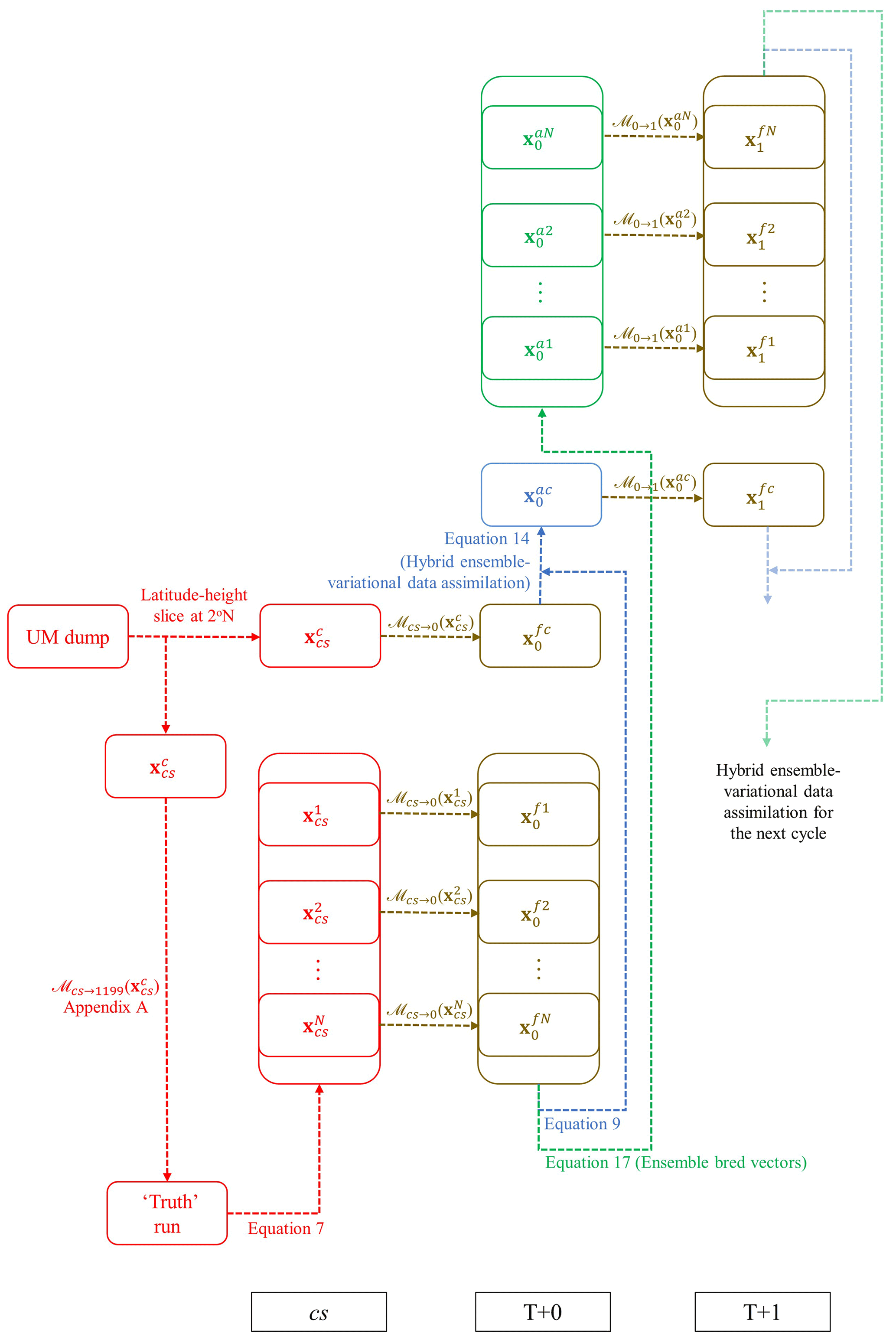
Figure 1 Schematic diagram of the ensemble and deterministic workflow for the hybrid-EnVar scheme in the ABC-DA system, illustrated for an hourly-cycling setup over the first cycle from a cold start. The subscripts refer to the validity time; cs refers to cold start. The superscripts fk and fc refer to the kth member of the forecast ensemble and the control forecast, respectively; and ak and ac refer to the kth member of the analysis ensemble and the hybrid control analysis, respectively.

3.1 Generation of initial ensemble of states for ABC ensemble system

This section discusses the generation of an initial ensemble, the first step in Fig. 1 (red segments) which is needed in the case of a cold start. Subsequent propagation of the ensemble can then proceed after this problem is addressed.

In the ABC model, an initial two-dimensional state can be computed from a longitude–height slice of a Unified Model output which is a convenient approach adopted by Petrie et al. (2017). In this light, the simplest method to generate an initial ensemble is to extract different longitude–height slices from the same Unified Model output, similar to how a population of training data is generated in Bannister (2020) for the calibration of the climatological background error covariances as mentioned in Sect. 2.2.2. Another method is to simply add statistical noise to the initial ABC model state, although it is not straightforward to determine the distributions for the noise sampling (which could vary for different variables and include multi-variate correlations), so that the solutions are consistent with the underlying dynamics. The model evolution in the first few cycles may spuriously dampen or amplify the added statistical noise if it is drawn from an incorrectly chosen distribution.

For this study, we adopt the random field perturbation method proposed by Magnusson et al. (2009) to generate the initial ensemble. The main idea relies on choosing two (assumed independent) ABC states and calculating their differences. The differences are treated as perturbations and can then be scaled to maintain a fixed amplitude between ensemble members and/or cycles, and are subsequently added to the initial ABC state computed above to generate an initial (arbitrary-sized) ensemble of states. Linear balances are approximately preserved in the resulting ensemble as only linear operations are performed on the fields (Magnusson et al., 2009).

Unlike in an operational NWP system where archived past analyses are available, a long “truth” simulation needs to be performed using the ABC model starting from a chosen initial state (the “truth run” in Fig. 1). To generate each ensemble member, two states from the same “truth” simulation are chosen at random. These need to be sufficiently separated in time for the assumption of independence to be valid. Following the above steps, the initial ensemble of states is given by

$$\begin{array}{}\text{(7a)}& {\displaystyle }{\mathit{x}}_{\mathrm{cs}}^k={\mathit{x}}_{\mathrm{cs}}^{\mathrm{c}}+{\displaystyle \frac{\mathrm{1}}{\sqrt{\mathrm{2}}}}{r}^k\left({\mathit{x}}_{kt\mathrm{1}}^{\mathrm{tr}}-{\mathit{x}}_{kt\mathrm{2}}^{\mathrm{tr}}\right),\text{(7b)}& {\displaystyle }{r}^k={\displaystyle \frac{{\mathit{ϵ}}^{\mathrm{rf}}}{|{\mathit{x}}_{kt\mathrm{1}}^{\mathrm{tr}}-{\mathit{x}}_{kt\mathrm{2}}^{\mathrm{tr}}{|}_{E_{\mathrm{tot}}}}},{\mathit{ϵ}}^{\mathrm{rf}}=\stackrel{\mathrm{‾}}{|{\mathit{x}}_{kt\mathrm{1}}^{\mathrm{tr}}-{\mathit{x}}_{kt\mathrm{2}}^{\mathrm{tr}}{|}_{E_{\mathrm{tot}}}},\end{array}$$

where ${\mathit{x}}_{\mathrm{cs}}^k$ represents the kth initial state of N ensemble members; ${\mathit{x}}_{\mathrm{cs}}^{\mathrm{c}}$ is the initial unperturbed (hereafter referred to as control) state; the subscript “cs” refers to cold start; ${\mathit{x}}_{kt\mathrm{1}}^{\mathrm{tr}}$ and ${\mathit{x}}_{kt\mathrm{2}}^{\mathrm{tr}}$ are the two random states drawn from the same “truth” simulation at different times (kt1 and kt2); and r^k depends on the scaling factor ϵ^rf defined according to the total energy norm ($|•{|}_{E_{\mathrm{tot}}}=\sqrt{E_{\mathrm{tot}}}$; see Eq. A1) of the perturbations to maintain a fixed amplitude (the ensemble mean $\stackrel{\mathrm{‾}}{|•{|}_{E_{\mathrm{tot}}}}$) between ensemble members. The reason for the $\frac{\mathrm{1}}{\sqrt{\mathrm{2}}}$ factor being included is because we are considering differences between two states so the variance of the difference is a reflection of the sum of their error variances rather than considering differences between a state and a mean (see Appendix of Berre et al., 2006). More details and justification of the method are covered in Appendix A.

After generating the initial ensemble, the cold start members are propagated to the analysis time of the first cycle at T+0 (from ${\mathit{x}}_{\mathrm{cs}}^k$ to ${\mathit{x}}_{\mathrm{0}}^{\mathrm{f}k}$ and from ${\mathit{x}}_{\mathrm{cs}}^{\mathrm{c}}$ to ${\mathit{x}}_{\mathrm{0}}^{\mathrm{fc}}$ by ℳ_cs→0; Fig. 1, lower brown segments). Note that for subsequent cycles, the analysis ensemble (produced from Sect. 3.3) and control analysis are propagated instead of cold start members (i.e. from ${\mathit{x}}_t^{\mathrm{a}k}$ to ${\mathit{x}}_{t+\mathrm{1}}^{\mathrm{f}k}$ and from ${\mathit{x}}_t^{\mathrm{ac}}$ to ${\mathit{x}}_{t+\mathrm{1}}^{\mathrm{fc}}$ by ${\mathcal{M}}_{t\to t+\mathrm{1}}$; Fig. 1, upper right brown segments). These ensemble forecasts are then used in the DA step, described in the next section.

3.2 Hybrid ensemble-variational data assimilation

The hybrid-EnVar approach seeks to implement a hybrid background error covariance B_h which is a linear combination of a climatological and an ensemble-derived background error covariance matrix (B_c and B_e) in the form following Hamill and Snyder (2000):

$$\begin{array}{}\text{(8)}& {\mathbf{B}}_{\mathrm{h}}={\mathit{\beta }}_{\mathrm{c}}^{\mathrm{2}}{\mathbf{B}}_{\mathrm{c}}+{\mathit{\beta }}_{\mathrm{e}}^{\mathrm{2}}{\mathbf{B}}_{\mathrm{e}},\end{array}$$

where ${\mathit{\beta }}_{\mathrm{c}}^{\mathrm{2}}$ and ${\mathit{\beta }}_{\mathrm{e}}^{\mathrm{2}}$ are (positive) scalar weights often determined empirically for the algorithm. These weights are often chosen to add to unity but this need not be the case. This approach computes B_h explicitly but is not practical in an NWP system. For the ABC-DA system, the alpha control variable approach of Lorenc (2003) is instead implemented which constructs an implied version of Eq. (8) using an alteration of the standard variational cost function and control variables (see Sect. 3.2.2). Wang et al. (2007) demonstrates the mathematical equivalence of both approaches.

Given the control background which is a short-range forecast from the previous cycle (${\mathit{x}}^{\mathrm{b}}={\mathit{x}}_t^{\mathrm{fc}}$), the hybrid-EnVar DA yields the hybrid control analysis ${\mathit{x}}_t^{\mathrm{ac}}$ (Fig. 1, blue segments) which needs the ensemble members to implicitly construct B_e (recall that B_c in Eq. 8 is derived from the U transform and B_e is derived from the ensemble). The steps to retrieve the hybrid control analysis are described in Sect. 3.2.2 but we first explain how B_e can be computed from the ensemble.

3.2.1 Computation of the ensemble-derived background error covariance matrix for the control analysis

At each cycle, one may compute a rectangular matrix ${\mathbf{X}}_t^{\mathrm{f}}$ whose columns contain the scaled differences between the ensemble forecasts (i.e. ${\mathit{x}}_t^{\mathrm{f}k}$ for the kth member forecast valid at time t) and the ensemble mean (${\stackrel{\mathrm{‾}}{\mathit{x}}}_t^{\mathrm{f}}$):

$$\begin{array}{}\text{(9)}& \begin{array}{rl}{\mathbf{X}}_t^{\mathrm{f}}& ={\displaystyle \frac{\mathrm{1}}{\sqrt{N-\mathrm{1}}}}\left({\mathit{x}}_t^{\mathrm{f}\mathrm{1}}-{\stackrel{\mathrm{‾}}{\mathit{x}}}_t^{\mathrm{f}},{\mathit{x}}_t^{\mathrm{f}\mathrm{2}}-{\stackrel{\mathrm{‾}}{\mathit{x}}}_t^{\mathrm{f}},\mathrm{\dots },{\mathit{x}}_t^{\mathrm{f}N}-{\stackrel{\mathrm{‾}}{\mathit{x}}}_t^{\mathrm{f}}\right)\\ & =\left({{\mathit{x}}^{\prime }}_t^{\mathrm{1}},{{\mathit{x}}^{\prime }}_t^{\mathrm{2}},\mathrm{\dots },{{\mathit{x}}^{\prime }}_t^N\right),\end{array}\end{array}$$

where ${{\mathit{x}}^{\prime }}_t^k$ are the scaled error modes valid at time t. The ensemble-derived background error covariance matrix (at time t) ${\mathbf{P}}_{\mathrm{e}}^{\mathrm{f}}\left[t\right]$ is explicitly given by the outer product:

$$\begin{array}{}\text{(10)}& {\mathbf{P}}_{\mathrm{e}}^{\mathrm{f}}\left[t\right]={\mathbf{X}}_t^{\mathrm{f}}{\mathbf{X}}_t^{\mathrm{f}\top }.\end{array}$$

As we shall see in Sect. 3.2.2, this matrix is not computed explicitly although parts of it are computed explicitly for visualisation purposes later in this article.

In the limit where N tends to infinity or where N is far greater than the degrees of freedom of the state n (N≫n), ${\mathbf{P}}_{\mathrm{e}}^{\mathrm{f}}\left[t\right]$ may be full rank. In practice, however, a small number of ensemble members (N≪n) will inevitably lead to sampling error and a rank-deficient matrix. Houtekamer and Mitchell (2001) proposed mitigating this problem by performing a Schur product of ${\mathbf{P}}_{\mathrm{e}}^{\mathrm{f}}$ with a correlation matrix (or localisation matrix) L:

$$\begin{array}{}\text{(11)}& {\mathbf{B}}_{\mathrm{e}}=\mathbf{L}\circ {\mathbf{P}}_{\mathrm{e}}^{\mathrm{f}}\left[t\right].\end{array}$$

This seeks to address the sampling error by damping the long-range background error covariances and effectively increasing the rank of ${\mathbf{P}}_{\mathrm{e}}^{\mathrm{f}}\left[t\right]$. The spatial and multi-variate aspects of the localisation matrix are further discussed in Sect. 3.2.3 including how this can be performed without constructing explicit matrices.

3.2.2 Alpha control variable transform

Following the approach of Lorenc (2003), we introduce an ensemble-related penalty in the variational cost function. This requires constructing so-called alpha fields α^k (part of a new set of mutually uncorrelated control variables) associated with each ensemble member k and constrained to have covariance L (the localisation matrix as used in Eq. 11). The number of elements in α^k must be the same as the state vector of ${{\mathit{x}}^{\prime }}_t^k$ (number of model grid points N_g × number of model variables N_var). The modified cost function is

$$\begin{array}{}\text{(12a)}& {\displaystyle }\begin{array}{rl}J& (\mathit{\delta }\mathit{\chi },{\mathit{\alpha }}^{\mathrm{1}},{\mathit{\alpha }}^{\mathrm{2}},\mathrm{\dots },{\mathit{\alpha }}^N)=\stackrel{J_{\mathrm{b}}}{\overbrace{{\displaystyle \frac{\mathrm{1}}{\mathrm{2}}}(\mathit{\delta }\mathit{\chi }-\mathit{\delta }{\mathit{\chi }}^{\mathrm{b}}{)}^{\top }(\mathit{\delta }\mathit{\chi }-\mathit{\delta }{\mathit{\chi }}^{\mathrm{b}})}}\\ & +\stackrel{J_{\mathrm{o}}}{\overbrace{{\displaystyle \frac{\mathrm{1}}{\mathrm{2}}}\sum _{t=\mathrm{0}}^T({\mathbf{H}}_t\mathit{\delta }\mathit{x}-\mathit{d}[t\left]{)}^{\top }{\mathbf{R}}_t^{-\mathrm{1}}\right({\mathbf{H}}_t\mathit{\delta }\mathit{x}-\mathit{d}\left[t\right])}}\\ & +\stackrel{J_{\mathrm{e}}}{\overbrace{{\displaystyle \frac{\mathrm{1}}{\mathrm{2}}}\sum _{k=\mathrm{1}}^N{\mathit{\alpha }}^{k\top }{\mathbf{L}}^{-\mathrm{1}}{\mathit{\alpha }}^k}}\end{array}\text{(12b)}& {\displaystyle }\text{with }\mathit{\delta }\mathit{x}={\mathit{\beta }}_{\mathrm{c}}\mathbf{U}\mathit{\delta }\mathit{\chi }+{\mathit{\beta }}_{\mathrm{e}}\sum _{k=\mathrm{1}}^N{{\mathit{x}}^{\prime }}_t^k\circ {\mathit{\alpha }}^k,\end{array}$$

where J_b, J_o, and J_e are the background, observation, and ensemble penalties, respectively. Equation (12) is an extension of Eq. (5) and Eq. (12b) is an extension of Eq. (4), the hybrid control variable transform. Together, these equations make up the hybrid scheme.

Similar to the way that B_c can be decomposed as ${\mathbf{B}}_{\mathrm{c}}={\mathbf{UU}}^{\top }$, L can be decomposed in terms of the alpha control variable transform, U^α, i.e. $\mathbf{L}={\mathbf{U}}^{\mathit{\alpha }}{\mathbf{U}}^{\mathit{\alpha }\top }$. Consider an alpha control vector χ^αk (again associated with ensemble member k) which is related to the alpha field α^k via

$$\begin{array}{}\text{(13)}& {\mathit{\alpha }}^k={\mathbf{U}}^{\mathit{\alpha }}{\mathit{\chi }}^{\mathit{\alpha }k}.\end{array}$$

Substituting Eq. (13) into Eq. (12) yields

$$\begin{array}{}\text{(14a)}& {\displaystyle }\begin{array}{rl}J(\mathit{\delta }\mathit{\chi },{\mathit{\chi }}^{\mathit{\alpha }\mathrm{1}},{\mathit{\chi }}^{\mathit{\alpha }\mathrm{2}},\mathrm{\dots },{\mathit{\chi }}^{\mathit{\alpha }N})& =J_{\mathrm{b}}+J_{\mathrm{o}}\\ & +{\displaystyle \frac{\mathrm{1}}{\mathrm{2}}}\sum _{k=\mathrm{1}}^N{\mathit{\chi }}^{\mathit{\alpha }k\top }{\mathit{\chi }}^{\mathit{\alpha }k}\end{array}\text{(14b)}& {\displaystyle }\text{with }\mathit{\delta }\mathit{x}={\mathit{\beta }}_{\mathrm{c}}\mathbf{U}\mathit{\delta }\mathit{\chi }+{\mathit{\beta }}_{\mathrm{e}}\sum _{k=\mathrm{1}}^N{{\mathit{x}}^{\prime }}_t^k\circ \left({\mathbf{U}}^{\mathit{\alpha }}{\mathit{\chi }}^{\mathit{\alpha }k}\right),\text{(14c)}& {\displaystyle }{\mathit{x}}_t^{\mathrm{ac}}={\mathit{x}}^{\mathrm{r}}+\mathit{\delta }{\mathit{x}}^{\mathrm{a}}.\end{array}$$

The variational problem (Eq. 14) is minimised with respect to the collective set of control vectors comprising a part that is associated with B_c (δχ) and parts that are associated with B_e (${\mathit{\chi }}^{\mathit{\alpha }\mathrm{1}},{\mathit{\chi }}^{\mathit{\alpha }\mathrm{2}},\mathrm{\dots },{\mathit{\chi }}^{\mathit{\alpha }N}$). Together, these are combined using the hybrid transform (Eq. 14b) to give the particular δx that minimises Eq. (14), namely, δx^a. This gives the analysis ${\mathit{x}}_t^{\mathrm{ac}}$ in Eq. (14c).

The total implied covariance matrix (that is effectively seen by the DA) is formally given by

$$\begin{array}{}\text{(15)}& {\mathbf{B}}_{\mathrm{h}}={\mathit{\beta }}_{\mathrm{c}}^{\mathrm{2}}{\mathbf{UU}}^{\top }+{\mathit{\beta }}_{\mathrm{e}}^{\mathrm{2}}\left({\mathbf{U}}^{\mathit{\alpha }}{\mathbf{U}}^{\mathit{\alpha }\top }\right)\circ \left({\mathbf{X}}_t^{\mathrm{f}}{\mathbf{X}}_t^{\mathrm{f}\top }\right),\end{array}$$

which is a linear combination of the implied B_c and B_e (without explicitly constructing either), and is element-wise equivalent to the explicit hybrid covariance in Eq. (8).

Next, we reproduce the minimisation algorithm steps Sect. 3.5 of Bannister (2020) and highlight (underlined) the modifications required when the hybrid-EnVar scheme is enabled.

1. Set the reference state at t=0 to the background state x^r=x^b. Decide values for N, β_c, and β_e;

2. Do the outer loop;

   • a.

     For the first outer loop, δχ^b=0; otherwise, compute $\mathit{\delta }{\mathit{\chi }}^{\mathrm{b}}={\mathbf{U}}^{-\mathrm{1}}({\mathit{x}}^{\mathrm{b}}-{\mathit{x}}^{\mathrm{r}})$,

   • b.

     Compute x^r[t] over the time window, $\mathrm{1}\le t\le T$, with the non-linear model ${\mathit{x}}^{\mathrm{r}}\left[t\right]={\mathcal{M}}_{t-\mathrm{1}\to t}\left({\mathit{x}}^{\mathrm{r}}\right[t-\mathrm{1}\left]\right)$,

   • c.

     Compute the reference state's observations: y^mr[t]=ℋ_t(x^r[t]),

   • d.

     Compute the differences: $\mathit{d}\left[t\right]=\mathit{y}\left[t\right]-{\mathit{y}}^{\mathrm{mr}}\left[t\right]$,

   • e.

     Set δχ=0, δx=0, and χ^αk=0, $\mathrm{1}\le k\le N$,

   • f.

     Do the inner loop,

     • i.

       Integrate the perturbation trajectory over the time window, $\mathrm{1}\le t\le T$, with the linear forecast model: $\mathit{\delta }\mathit{x}\left[t\right]={\mathbf{M}}_{t-\mathrm{1}\to t}\mathit{\delta }\mathit{x}[t-\mathrm{1}]$

     • ii.

       Compute the perturbations to the model observations: δy^m[t]=H_tδx[t]

     • iii.

       Compute Δ[t] vectors as defined as $\mathbf{\Delta }\left[t\right]={\mathbf{H}}_t^{\top }{\mathbf{R}}_t^{-\mathrm{1}}\left(\mathit{\delta }{\mathit{y}}^{\mathrm{m}}\right[t]-\mathit{d}[t\left]\right)$

     • iv.

       Set the adjoint state $\mathit{\lambda }[T+\mathrm{1}]=\mathrm{0}$

     • v.

       Integrate the following adjoint equation backwards in time $T\ge t\ge \mathrm{0}$: $\mathit{\lambda }\left[t\right]=\mathbf{\Delta }\left[t\right]+{\mathbf{M}}_{t\to t+\mathrm{1}}^{\top }\mathit{\lambda }[t+\mathrm{1}]$

     • vi.

       Compute the gradient as follows: ${\mathrm{\nabla }}_{\mathit{\delta }\mathit{\chi }}J=\mathit{\delta }\mathit{\chi }-\mathit{\delta }{\mathit{\chi }}^{\mathrm{b}}+{\mathit{\beta }}_{\mathrm{c}}{\mathbf{U}}^{\top }\mathit{\lambda }\left[\mathrm{0}\right]$, and ${\mathrm{\nabla }}_{{\mathit{\chi }}^{\mathit{\alpha }k}}J={\mathit{\chi }}^{\mathit{\alpha }k}+{\mathit{\beta }}_{\mathrm{e}}{\mathbf{U}}^{\mathit{\alpha }\top }({{\mathit{x}}^{\prime }}_t^k\circ \mathit{\lambda }[\mathrm{0}\left]\right)$; these are the gradients with respect to each control vector segment, $\mathrm{1}\le k\le N$

     • vii.

       Use the conjugate gradient algorithm to adjust δχ and χ^αk to reduce the value of J. Note that the cost function is $J=J_{\mathrm{b}}+J_{\mathrm{o}}+J_{\mathrm{e}}$ (Eq. 14)

     • viii.

       Compute the new increment in model space using the control variable transform and alpha control variable transform: $\mathit{\delta }\mathit{x}={\mathit{\beta }}_{\mathrm{c}}\mathbf{U}\mathit{\delta }\mathit{\chi }+{\mathit{\beta }}_{\mathrm{e}}{\sum }_{k=\mathrm{1}}^N{{\mathit{x}}^{\prime }}_t^k\circ \left({\mathbf{U}}^{\mathit{\alpha }}{\mathit{\chi }}^{\mathit{\alpha }k}\right)$ (Eq. 14b)

     • ix.

       Go to step 2fi until the inner-loop convergence criterion is satisfied

   • g.

     Update the reference state: ${\mathit{x}}^{\mathrm{r}}\to {\mathit{x}}^{\mathrm{r}}+\mathit{\delta }\mathit{x}$,

   • h.

     Go to step 2a until the outer-loop convergence criterion is satisfied. At convergence, set the hybrid control analysis ${\mathit{x}}_t^{\mathrm{ac}}={\mathit{x}}^{\mathrm{r}}$,

3. Run a non-linear forecast from ${\mathit{x}}_t^{\mathrm{ac}}$ for the background of the next cycle and longer forecasts if required.

3.2.3 Inter-variable and spatial localisation

Localisation of the ensemble-derived background error covariance matrix, as in Eq. (11), is required to mitigate sampling error which can dominate the computed covariance between distant points (Hamill et al., 2001). Localisation opens up a range of options and raises some pertinent questions: should we localise only in space (and should these spatial localisation matrices depend on the variable) or should we additionally include localisation between different model variables? This depends on the design of χ^αk and U^α in Eq. (13), and the implied L. If χ^αk only depends on grid point location (i.e. it need only be of length N_g), then U^α must be rectangular (N_gN_var×N_g) so that α^k has length N_gN_var required for the Schur product in Eq. (12b). This approach was adopted by Wang et al. (2008a) except that χ^αk was only dependent on horizontal grid point locations. By design, U^α functions to “use the same χ^αk for each model variable and model level” (i.e. repeated rows in U^α) so the Schur product in Eq. (14b) can be computed. This point was not highlighted in the description of Eq. (1) of Wang et al. (2008a).

If χ^αk only has N_g elements, the implied $\mathbf{L}={\mathbf{U}}^{\mathit{\alpha }}{\mathbf{U}}^{\mathit{\alpha }\top }$ can only involve spatial localisation so full inter-variable covariances (as found from the raw ensemble) are retained (see Appendix B). Alternatively, if χ^αk is full length (i.e. of length N_gN_var) with independent fields for each model variable, U^α is square (N_gN_var×N_gN_var) so it is possible to use this transform to damp the ensemble-derived covariances between different variables and spatial locations. Nonetheless, there is flexibility to still retain the full inter-variable covariances in L depending on the design of U^α. For the record, a proof of the equivalence between this approach (χ^αk with length N_gN_var) with full inter-variable covariances retained, and the approach where χ^αk is of length N_g is included in Appendix B. More complex designs of U^α which allow the retention of inter-variable covariances only between certain model variables or using different spatial localisation length-scales for different model variables are also possible. In practice, these may be useful in convective-scale data assimilation particularly when hydrometeor variables are involved (Xuguang Wang, personal communication, 2022).

In the ABC-DA system, U^α is further decomposed into the horizontal ${\mathbf{U}}_{\mathrm{horiz}}^{\mathit{\alpha }}$ and vertical ${\mathbf{U}}_{\mathrm{vert}}^{\mathit{\alpha }}$ localisation transforms similar to the decomposition of U in Bannister (2020). The series of transforms is given by

$$\begin{array}{}\text{(16)}& {\mathbf{U}}^{\mathit{\alpha }}={\mathbf{U}}_{\mathrm{vert}}^{\mathit{\alpha }}{\mathbf{U}}_{\mathrm{horiz}}^{\mathit{\alpha }},\end{array}$$

treating the vertical and horizontal localisation separately.

Initial tests constructed ${\mathbf{U}}_{\mathrm{horiz}}^{\mathit{\alpha }}$ using a Fourier decomposition (as is done in the standard horizontal transform of U – see Bannister, 2020), but this yielded undesirable small negative correlations at longer localisation distances (presumably related to the Gibbs phenomenon; not shown). Thus, a different approach was adopted as the basis for populating ${\mathbf{U}}_{\mathrm{horiz}}^{\mathit{\alpha }}$ using the eigendecomposition of a target horizontal localisation matrix ${\mathbf{L}}_{\mathrm{horiz}}={\mathbf{U}}_{\mathrm{horiz}}^{\mathit{\alpha }}{\mathbf{U}}_{\mathrm{horiz}}^{\mathit{\alpha }\top }$ (where ${\mathbf{U}}_{\mathrm{horiz}}^{\mathit{\alpha }}={\mathbf{F}}_{\mathrm{horiz}}^{\mathit{\alpha }}({\mathbf{\Lambda }}_{\mathrm{horiz}}^{\mathit{\alpha }}{)}^{\mathrm{1}/\mathrm{2}}$, and ${\mathbf{F}}_{\mathrm{horiz}}^{\mathit{\alpha }}$ and ${\mathbf{\Lambda }}_{\mathrm{horiz}}^{\mathit{\alpha }}$ are the eigenvectors and eigenvalues, respectively, of the imposed horizontal localisation matrix). We start by constructing L_horiz using the fifth-order piecewise Gaspari–Cohn function with a horizontal localisation length-scale h^α (equivalent to c with $a=\mathrm{1}/\mathrm{2}$, in Eq. 4.10 of Gaspari and Cohn, 1999). This function is approximately Gaussian over a compact support. As the ABC model uses periodic boundary conditions, L_horiz must be designed to be circulant and account for “overlapping tails” of the Gaspari–Cohn function when h^α is larger than half the domain size. In the “overlapping tails” regime, the correlation function does not satisfy the “space-limited” requirement described in (Gaspari and Cohn, 1999). Thus, the resulting L_horiz is found to not be positive semi-definite when h^α is large and tends to infinity so the horizontal eigenvectors associated with the negative eigenvalues need to be truncated. Offline testing in idealised setups and within the ABC-DA system showed that with the remaining eigenvectors, ${\mathbf{U}}_{\mathrm{horiz}}^{\mathit{\alpha }}{\mathbf{U}}_{\mathrm{horiz}}^{\mathit{\alpha }\top }$ is a good approximation for L_horiz. It is also possible to scale the remaining eigenvalues to restore the initial total variances for a better approximation. Figure 2 illustrates the implied correlation function (h^α=250 km) with respect to longitudinal grid point 50 for an ABC-DA system with 364 longitudinal grid points and a 1.5 km horizontal grid retrieved using the above steps. The original Gaspari–Cohn function with “overlapping tails” is compared with the implied correlation function reconstructed from the eigenvectors and eigenvalues of the eigendecomposition of L_horiz (Fig. 2a), the resulting implied correlation function when negative eigenvectors/eigenvalues are truncated (Fig. 2b) and the resulting implied correlation function after further restoration of the initial total variances by scaling (Fig. 2c). Note that in this example, the threshold for which negative eigenvalues appear is h^α≈138.33 km found empirically. In the current version of the ABC-DA system, the scaling to restore initial total variances is not implemented yet.

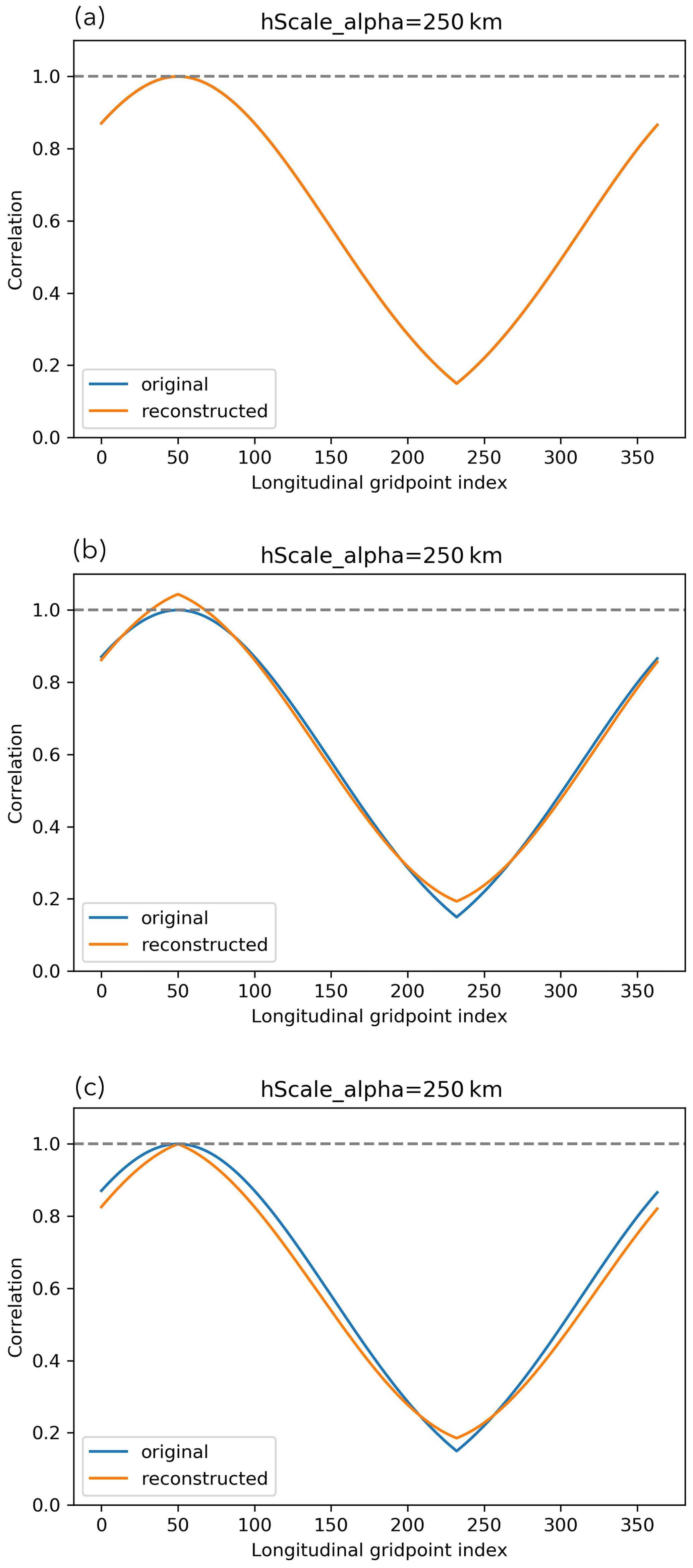
Figure 2 Correlation functions (h^α=250 km) with respect to longitudinal grid point 50 for an ABC-DA system with 364 longitudinal grid points and 1.5 km horizontal grid. The implied correlation functions (orange) are reconstructed from (a) all eigenvectors and eigenvalues of the eigendecomposition of L_horiz, (b) only eigenvectors with non-negative eigenvalues, (c) only eigenvectors with non-negative eigenvalues that are scaled to restore initial total variance, and compared with the original Gaspari–Cohn function (blue).

To populate ${\mathbf{U}}_{\mathrm{vert}}^{\mathit{\alpha }}$, a similar approach is adopted; a Gaspari–Cohn function is used with vertical localisation length-scale v^α. Note that the target vertical localisation matrix L_vert is a correlation matrix and so must be positive semi-definite so truncation of eigenvectors is not required. Since ${\mathbf{U}}_{\mathrm{horiz}}^{\mathit{\alpha }}$ and ${\mathbf{U}}_{\mathrm{vert}}^{\mathit{\alpha }}$ are separate, it is possible to have a different L_vert for each horizontal eigenvector. However, for simplicity, the default setup in the ABC-DA system uses the same L_vert for each horizontal eigenvector. As for L_horiz, the vertical eigenvectors are retrieved through the eigendecomposition of L_vert and used to populate ${\mathbf{U}}_{\mathrm{vert}}^{\mathit{\alpha }}$ such that ${\mathbf{L}}_{\mathrm{vert}}={\mathbf{U}}_{\mathrm{vert}}^{\mathit{\alpha }}{\mathbf{U}}_{\mathrm{vert}}^{\mathit{\alpha }\top }$ (where ${\mathbf{U}}_{\mathrm{vert}}^{\mathit{\alpha }}={\mathbf{F}}_{\mathrm{vert}}^{\mathit{\alpha }}({\mathbf{\Lambda }}_{\mathrm{vert}}^{\mathit{\alpha }}{)}^{\mathrm{1}/\mathrm{2}}$, and ${\mathbf{F}}_{\mathrm{vert}}^{\mathit{\alpha }}$ and ${\mathbf{\Lambda }}_{\mathrm{vert}}^{\mathit{\alpha }}$ are the eigenvectors and eigenvalues, respectively, of the imposed vertical localisation matrix).

3.3 Generation of ABC analysis ensemble

After the initial ensemble has been generated (Sect. 3.1) using the method of Magnusson et al. (2009) and the initial hybrid control analysis has been retrieved (Sect. 3.2), the next step is to generate analysis ensembles (Fig. 1, green segments). The ensemble then proceeds via the forecast model (Fig. 1, upper right brown segments) as a forecast ensemble which is used in the next hybrid DA step. Various methods have been used in previous studies, such as singular vectors (Buizza et al., 1993), bred vectors (Toth and Kalnay, 1993, Toth and Kalnay, 1997), perturbed observations (Houtekamer and Derome, 1995), EnKF (Evensen, 1994), ensemble transform Kalman filter (Bishop et al., 2001), and other square root filters. Here, we focus mainly on the EBV method. This method has useful information about the nature of dynamical error growth about the analysis state at each cycle but is uninformed about the observation network.

The ensemble, which is run in parallel to the hybrid DA, are important components in hybrid-EnVar since they provide the means to compute ${\mathbf{X}}_t^{\mathrm{f}}$ in Eq. (9). The success of the scheme depends on the extent to which the ensemble forecasts can appropriately represent the background error statistics for the ABC-DA system so proper design of the ensemble system is critical. We construct the analysis ensemble around the hybrid control analysis (i.e. adding ensemble perturbations to the hybrid control analysis; see below) so the ensemble is “DA-centred”.

3.3.1 Ensemble bred vectors

In this approach, we consider a variant of the bred vectors method – the EBV method (Balci et al., 2012). The basic bred vectors method (Toth and Kalnay, 1993) is generally simple to implement and has a cheap computational cost. The idea relies on breeding perturbations by running the non-linear forecast model for a fixed period for pairs of forecast ensemble members, taking the difference between the two forecasts, and then scaling the difference to have a specified and fixed amplitude. This process “breeds” the fastest growing error modes. This is repeated to retrieve the required number of error modes and the resulting perturbations are respectively added to the hybrid control analysis to generate an analysis ensemble. The intention is that these perturbations should adequately sample the space of possible analysis errors.

The main difference between the bred vectors and EBV methods lies in the scaling of the perturbations at each cycle. In the bred vectors method, the perturbations are scaled to maintain a fixed amplitude across cycles for each ensemble member. The scaling is independent for each ensemble member and there is, therefore, no mechanism to compare the dynamics with perturbations of the other members. The EBV method (Balci et al., 2012), on the other hand, involves a global scaling factor which depends on the amplitude of the largest perturbation and offers better insights into the relative behaviour of nearby ensemble trajectories. Perturbations that have an amplitude smaller than the largest perturbation of the ensemble then play a smaller role after scaling; in other words, ensemble trajectories that are clustered around the control member trajectory are less important for identifying dominant directions of error growth. An in-depth comparison of the bred vectors and EBV methods is provided in Balci et al. (2012).

To generate the analysis ensemble, a target maximum amplitude ϵ₀ is required but this opens the question on what to choose for ϵ₀. Here, we use ϵ₀=ϵ^rf (the mean total energy norm of the initial ensemble of states) although other choices are possible, such as running a series of experiments and finding the average analysis error to estimate the analysis uncertainty. This scaling factor is fixed across perturbations so at each cycle, the perturbations are scaled by the same ratio $r_t^{\mathrm{ebv}}$ which is used and defined as follows:

$$\begin{array}{}\text{(17a)}& {\displaystyle }\begin{array}{rl}\mathit{\delta }{\mathit{x}}_t^{\mathrm{f}k}& ={\displaystyle \frac{\mathrm{1}}{\sqrt{\mathrm{2}}}}{r}_t^{\mathrm{ebv}}({\mathit{x}}_t^{\mathrm{f}k}-{\mathit{x}}_t^{\mathrm{fc}}),\\ & r_t^{\mathrm{ebv}}={\displaystyle \frac{{\mathit{ϵ}}_{\mathrm{0}}}{\text{max}\left[\right|{\mathit{x}}_t^{\mathrm{f}k}-{\mathit{x}}_t^{\mathrm{fc}}{|}_{E_{\mathrm{tot}}}]}},\end{array}\text{(17b)}& {\displaystyle }{\mathit{x}}_t^{\mathrm{a}k}={\mathit{x}}_t^{\mathrm{ac}}+\mathit{\delta }{\mathit{x}}_t^{\mathrm{f}k},\end{array}$$

where ${\mathit{x}}_t^{\mathrm{f}k}$ and ${\mathit{x}}_t^{\mathrm{fc}}$ are the kth ensemble and control forecast from the previous cycle, respectively, and $\mathit{\delta }{\mathit{x}}_t^{\mathrm{f}k}$ is the kth scaled ensemble perturbation at time t. The kth member of the analysis ensemble ${\mathit{x}}_t^{\mathrm{a}k}$ is centred on the hybrid control analysis ${\mathit{x}}_t^{\mathrm{ac}}$ produced by the DA step (Sect. 3.2). The $\frac{\mathrm{1}}{\sqrt{\mathrm{2}}}$ factor is not necessarily required because we are computing differences between individual ensemble member forecasts and the same control member forecast, but we have included it as a deflation factor with our choice of ϵ₀. It is worth noting that the EBV method is not formally consistent with Kalman filter theory but will not suffer from filter collapse as long as the ϵ₀ chosen is well-tuned.

It is not uncommon to use such a set-up (i.e. separate hybrid deterministic and ensemble systems for, respectively, the first and second moments of the posterior). While the hybrid control analysis involves both the ensemble and climatological contributions to the background error covariance matrix Eq. (15), the computation of analysis perturbations involves only the forecast ensemble and neglects the climatological contributions. While this is a formal discrepancy, we assume that this setup is an adequate from a practical perspective.

4 Data assimilation experiments using the hybrid-EnVar scheme in a tropical setting

For this study, the Unified Model output is retrieved from a tropical convective-scale NWP system over the Maritime Continent (SINGV-DA; Heng et al., 2020). SINGV-DA operates on a 1.5 km core horizontal grid with a model top height of 38.5 km. Longitude–height slices of fields u and v around 2^∘ N are extracted from the SINGV-DA output by placing these fields onto the 1.5 km ABC model grid for the lowest 60 levels (up to around 18 km height), resulting in a 364×60 ABC model grid. These initial u and v fields are then modified to make them compatible with the ABC model's periodic boundary conditions and the remaining fields, w, ${\stackrel{\mathrm{̃}}{\mathit{\rho }}}^{\prime }$, and b^′, are derived following the procedure in Sect. 4.1 of Bannister (2020). For the ensemble system, 30 initial ensemble members are generated following Sect. 3.1 excluding the control state reconfigured from the longitude–height slice. This is a typical ensemble size used in operational NWP systems.

To represent a tropical setting of the ABC model, a value of $f={\mathrm{10}}^{-\mathrm{5}}$ s⁻¹ is used. This corresponds approximately to a value of f at a latitude of 4^∘ N in an NWP system. The other model parameters are set as follows: A=0.02 s⁻¹, B=0.01, and C=10⁴ m² s⁻². A series of hourly-cycling multi-cycle DA observation system simulation experiments are conducted to demonstrate the incorporation of ensemble-derived background error covariances in hybrid-EnVar DA. The hybrid extension of 3DVar-FGAT may be termed hybrid-En3DVar-FGAT.

We run four experiments with the following configurations:

• a.

  100 % B_c (i.e. no flow-dependency, equivalent to 3DVar-FGAT),

• b.

  50 % B_c, 50 % B_e; hybrid-En3DVar-FGAT (i.e. flow-dependency with an equal contribution from B_c and B_e),

• c.

  20 % B_c, 80 % B_e; hybrid-En3DVar-FGAT (i.e. flow-dependency with most contribution from B_e),

• d.

  100 % B_e; pure En3DVar-FGAT (i.e. no contribution from B_c).

These experiments are referred to as EBV(a) to EBV(d) accordingly. Note that configuration (a) does not use ensemble information but the experiment is named as EBV(a) for ease of reference.

4.1 Implied background error covariances

To show the workings of Eq. (8) (or equivalently Eq. 15) and the localisation, we compute a selection of implied background error covariances with the various weights assigned to B_c and B_e (as the above configurations (a) to (d)). This is similar to performing single observation experiments and retrieving the analysis increments. For B_e, spatial localisation length scales of h^α=100 km and v^α=5 km are set, and with no inter-variable localisation. The implied background error covariances are valid for the time of the first cycle after a cold start (i.e. at T+0) and use 1 h forecast ensemble perturbations. For B_c, the same ensemble is used as training data to calibrate U.

Figure 3 shows the implied background error covariances of ${\stackrel{\mathrm{̃}}{\mathit{\rho }}}^{\prime }$, v, and b^′ with respect to a fixed ${\stackrel{\mathrm{̃}}{\mathit{\rho }}}^{\prime }$ point in the middle of the domain for the four configurations (four rows). Configuration (a) (top row) shows the implied background error covariances that are modelled purely by U and configuration (d) (bottom row) shows the purely ensemble-derived covariances with spatial localisation (implied by U^α). Configurations (b) and (c) are linear combinations with different weights as demonstrated by Eq. 8.

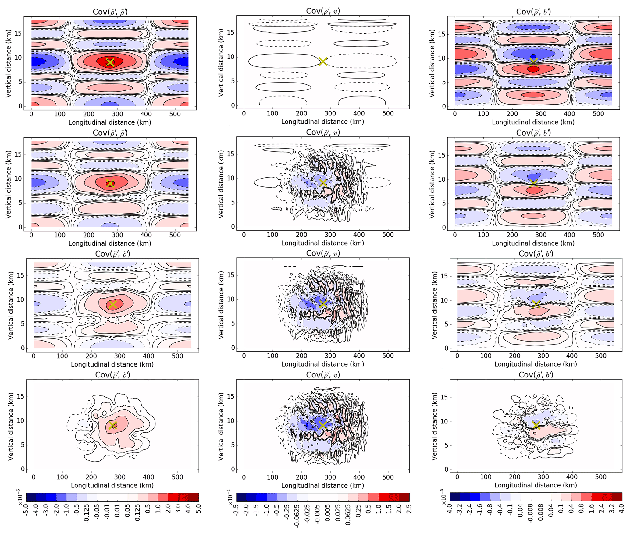
Figure 3 Implied background error covariances of ${\stackrel{\mathrm{̃}}{\mathit{\rho }}}^{\prime }$ (leftmost column; Cov(${\stackrel{\mathrm{̃}}{\mathit{\rho }}}^{\prime }$, ${\stackrel{\mathrm{̃}}{\mathit{\rho }}}^{\prime }$)), v (middle column; Cov(${\stackrel{\mathrm{̃}}{\mathit{\rho }}}^{\prime }$, v)) and b^′ (rightmost column; Cov(${\stackrel{\mathrm{̃}}{\mathit{\rho }}}^{\prime }$, b^′)) with respect to a ${\stackrel{\mathrm{̃}}{\mathit{\rho }}}^{\prime }$ point (yellow cross) near the centre of the domain for the first cycle after cold start. The rows represent configurations (a), (b), (c), and (d), respectively (see the list near the start of Sect. 4). Negative values have contours that are dashed.

For ${\stackrel{\mathrm{̃}}{\mathit{\rho }}}^{\prime }$–${\stackrel{\mathrm{̃}}{\mathit{\rho }}}^{\prime }$ covariances in configuration (a) for pure 3DVar-FGAT, the central region of auto-correlation has horizontal and vertical length scales of  100 and  2 km, respectively, and is surrounded by oscillations possibly reflecting the dominant gravity wave propagation. The vertical length scale here is smaller than that found in the mid-latitude study of Bannister (2020), and such a contrast between low and higher latitudes is seen in other studies, e.g. Ingleby (2001). This can be compared with configuration (d) for pure (and localised) En3DVar-FGAT which shows a narrower but taller region of auto-correlation. Most of the oscillations are beyond the localisation region so are not visible apart from small negative values to the west of the auto-correlation.

The ${\stackrel{\mathrm{̃}}{\mathit{\rho }}}^{\prime }$–v covariances in configuration (a) follow from the use of geostrophic balance which is manifested in U (Eq. 2a in Bannister, 2020). The v pattern is consistent with an anti-cyclonic field around the source point (i.e. positive and negative v covariances west and east of the positive ${\stackrel{\mathrm{̃}}{\mathit{\rho }}}^{\prime }$ source point, respectively). Since f is small, these covariances are also small. Contrasting this with configuration (d), it appears that the ensemble-derived covariances are more substantial and are of opposite sign suggesting that there exists some (other) mass–wind relationship manifested in B_e (e.g. related to equatorial gravity wave processes not represented in U).

The ${\stackrel{\mathrm{̃}}{\mathit{\rho }}}^{\prime }$–b^′ covariances in configuration (a) follow from the use of hydrostatic balance, again manifested in U (Eq. 3 in Bannister, 2020). Hydrostatic balance relates b^′ increments with the vertical gradient of ${\stackrel{\mathrm{̃}}{\mathit{\rho }}}^{\prime }$ increments, and the top-left and top-right panels are confirmed to be consistent in this way. In configuration (d), the ${\stackrel{\mathrm{̃}}{\mathit{\rho }}}^{\prime }$–b^′ covariances have similar vertical patterns within the localisation region although they are weaker. As noted in Bannister (2020), the B_c covariances tend to be larger than their B_e counterparts even though both use the same training data for calibrating the transforms, but the broad structures are similar.

Note that the implied background error covariances between ${\stackrel{\mathrm{̃}}{\mathit{\rho }}}^{\prime }$ and u and w are each zero in configuration (a) by definition of U (Bannister, 2020). By contrast, in configurations (b), (c), and (d), the implied background error covariances are prescribed directly between the associated model variables implied by U^α (not shown).

Even though the multi-variate background error relationships relevant to the tropics are likely to be different from those at mid-latitudes, the same balance conditions designed for mid-latitudes are often used in U for tropical settings (as they are here). By exploring ensemble-derived multi-variate background error relationships, we may be able to identify alternative balances inherent in the dynamical fields. This will be explored in a separate study.

4.2 Details of observation system simulation experiments

In all experiments, 200 observations of each variable (u, v, w, ${\stackrel{\mathrm{̃}}{\mathit{\rho }}}^{\prime }$, and b^′), which are equally spaced throughout the domain, are assimilated at every hourly cycle. The observations are sampled from a “truth” run with added observation noise following a Gaussian distribution. The observation error standard deviations are chosen to be approximately 10 % of the variable's root mean square value as seen in the “truth” run. These are 0.2, 0.2, 0.01, $\mathrm{1.5}\times {\mathrm{10}}^{-\mathrm{4}}$, and $\mathrm{1.5}\times {\mathrm{10}}^{-\mathrm{3}}$ m s⁻² for u, v, w, ${\stackrel{\mathrm{̃}}{\mathit{\rho }}}^{\prime }$, and b^′, respectively. All generated observations are valid at the background/analysis time of each cycle so there is no difference in the analysis between 3DVar and 3DVar-FGAT (and indeed, 4DVar, if it were implemented). The number of observations are ≈1 % of the degrees of freedom of the state (both spatial and multi-variate) to mimic how observations are sparse in the tropical setting.

The initial background of the deterministic system is determined from the initial “truth” plus a small background noise perturbation δx=Uδχ, where δχ is drawn randomly from 𝒩(0,I). In order to reduce the effect of random noise on the experiments, the ABC-DA system is first spun-up for fifty 1 h cycles with the expectation that the DA-centred ensemble system and deterministic system will have lost memory of the particular way that the system was initialised from a cold start. The information from the 50th cycle of spin-up is then used in the first cycle of all the actual experiments.

During the spin-up configuration testing, we noticed that the inclusion of vertical localisation in B_e was particularly detrimental to the evolution of the w field. Investigation revealed that this was due to the introduction of hydrostatic imbalance in the analysis increments (not shown). A similar well-known issue to do with horizontal localisation introducing geostrophic imbalance was discussed in Sect. 3c of Lorenc (2003). We include more comments on the hydrostatic imbalance issue in Appendix C. For this reason, vertical localisation was excluded in B_e in the spin-up process and in all experiments. After inspecting the other fields during spin-up configuration testing, we found that in most configurations, the hybrid control analysis gradually converged around the “truth” run as the observations were assimilated over the 50 spin-up cycles, as logically expected. Particularly using the EBV(d) configuration, the evolution of the fields was reasonably in line with the “truth” run so this was the chosen configuration which was run for 50 spin-up cycles, referred to as the spin-up run.

To ensure a fair comparison in the results, the spin-up run provides the same starting background (50th cycle forecast), empirically tuned EBV ensemble, and ensemble-derived error modes (if required) for the first cycle of all the actual experiments. Each experiment is run for 50 cycles and only differ in the DA algorithm configurations after spin-up. Where B_e is required, we use h^α=20 km for the horizontal localisation while not performing any inter-variable localisation (see Appendix B). The horizontal localisation length-scale was determined by comparing with the horizontal distance between adjacent observations (≈23 km). For the minimisation, a total of 75 inner loops within a single outer loop is used. This was determined after testing to ensure that sufficient convergence was attained for all cycles in the experiments. This is demonstrated in Fig. 4 which shows the minimisation of the cost function for the first cycle of the EBV experiments. For this cycle, the cost function was minimised the fastest and slowest in EBV(d) and (a), respectively. The analysis misfit to assimilated observations was also the largest in EBV(d) with J_o≈1500 after minimisation. However, it is important to note that this metric is not a particularly useful indicator of analysis quality but rather how each scheme draws the analysis towards the observations (Wang et al., 2008b). We would expect that the minimum of the cost function would approximate half the number of observations (i.e. $J_{\min }\approx \frac{N_{\mathrm{obs}}}{\mathrm{2}}=\mathrm{500}$, the expected value of a chi-squared PDF), so EBV(c) neatly matches our expectations.

In addition to the experiments, a free background run, hereafter referred to as FreeBG, is performed starting from the same 50th cycle forecast of the spin-up run. This is used as the control run to assess if the DA in the experiments is adding value by bringing the deterministic run trajectories closer to the “truth” or if the trajectories are simply following the natural evolution of the system and neglecting the observational information.

Figure 4 Total penalty (black) from the climatological background (blue), ensemble background (green), and observation (red) penalty contributions over the 75 inner loops for the first cycle of the EBV experiments, labelled (a) to (d) accordingly. Early termination of inner loops occurs when convergence criteria is satisfied, in (c) and (d). At convergence, ensemble penalty (green) in (b) and (c) is around 1.5 and 7, respectively.

4.3 Sensitivity to weighting of B_c and B_e

Typically, for the hybrid-EnVar scheme, tuning of the weights (${\mathit{\beta }}_{\mathrm{c}}^{\mathrm{2}}$ and ${\mathit{\beta }}_{\mathrm{e}}^{\mathrm{2}}$) for B_c and B_e is performed empirically to assess the best configuration which combines the benefits from both sources of background error statistics. Figure 5 shows the comparison of domain-averaged analysis errors (root mean square errors; RMSE) with respect to the “truth” for the EBV and FreeBG experiments.

The cycle-averaged analysis errors (Fig. 5; bottom right panel) for all prognostic variables except v are generally smaller for the EBV experiments compared to FreeBG with an RMSE ratio less than 1. During the simulation, the w, ${\stackrel{\mathrm{̃}}{\mathit{\rho }}}^{\prime }$, and b^′ errors were decreasing, suggesting that the deterministic run trajectories of the EBV experiments were converging around the “truth” because of the availability of observational information. The u analysis errors were decreasing in EBV(c) and EBV(d) but were increasing in EBV(a) and EBV(b). Throughout the 50 cycles, the v analysis errors were generally increasing in the EBV experiments. This peculiar issue was exacerbated when the weighting towards B_c was increased, suggesting that the issue originates from B_c. A feature of the u, ${\stackrel{\mathrm{̃}}{\mathit{\rho }}}^{\prime }$, and b^′ RMSE time sequences is the 8 h periodicity which is also apparent in the basic dynamical root mean square fields. A normal mode analysis (not shown) and inspection of the basic dynamical fields reveals that there is a 16 h period (local maxima to local maxima) which is within the period range of low-zonal-wavenumber gravity waves, suggesting that this feature is due to the dominant gravity waves in this system.

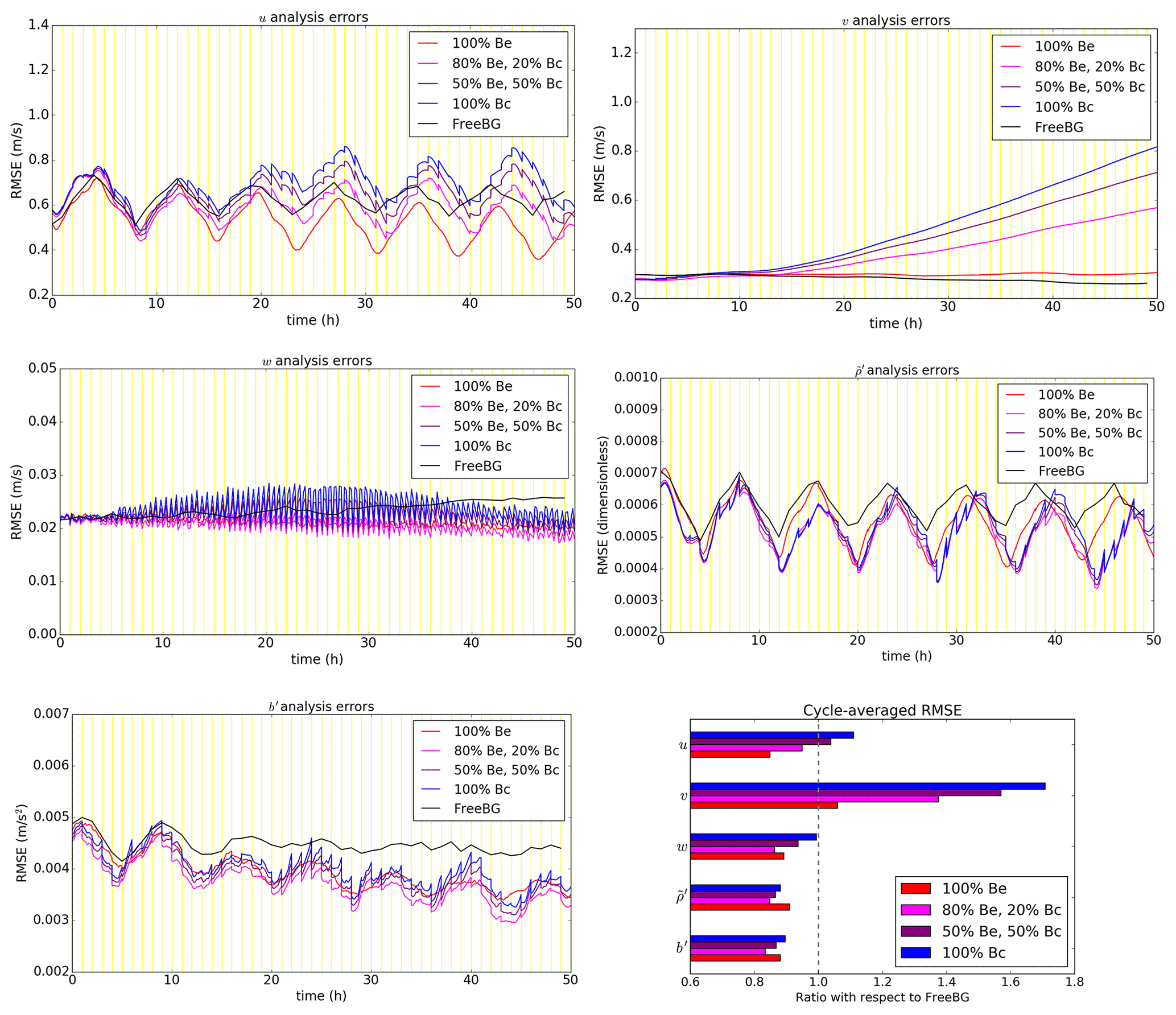
Figure 5 All panels except bottom right: time series of root mean square analysis errors for the EBV experiments (100 % B_c, configuration EBV(a); 50 % B_e, 50 % B_c, EBV(b); 80 % B_e, 20 % B_c, EBV(c); 100 % B_e, EBV(d)) and the free background run (FreeBG). The vertical yellow lines are the analysis times. Analysis errors are defined with respect to the “truth” run computed every 10 min within the respective assimilation windows for EBV experiments and every hour for FreeBG. Bottom right: the ratio of the cycle-averaged RMSE of the EBV experiments with respect to FreeBG for the five ABC model variables.

To test if the issue with the v analysis errors was due to the choice of training data, we repeated EBV(a) but with B_c calibrated using other training data (e.g. the ensemble perturbations from the 50th cycle of the spin-up run instead of those from the initial forecast ensemble). Even with more time-appropriate training data (but same variances), the issue was only partially resolved (smaller increase in RMSE; not shown). Also, this issue does not appear to occur in mid-latitudinal experimental setups in Bannister (2021). From the implied background error covariances in Sect. 4.1, there exists some mass–wind relationship in B_e that is not well-represented in B_c through the geostrophic balance relationship since f is small in the tropical setting. Repeating EBV(a) but omitting the geostrophic balance constraint entirely in the calibration of B_c (i.e. treating ${\stackrel{\mathrm{̃}}{\mathit{\rho }}}^{\prime }$ and v background errors univariately), also did not resolve the issue (not shown). We speculate that the issue could be due to the absence of a suitable balance constraint for prescribing the mass–wind relationship for B_c or a likely lack of tuning of the variances for B_c. Early results with a tuned B_c showed that the issue with the v analysis errors could be resolved by reducing the variances of all variables substantially. This warrants further investigation in a separate study to tune the variances for the system or assess the possibility of deriving a balance relationship between v and ${\stackrel{\mathrm{̃}}{\mathit{\rho }}}^{\prime }$ for the tropical setting.

Comparing between the EBV experiments, the u analysis errors and v analysis errors are generally the smallest in EBV(d), indicating that allocating full weight to B_e in this setup is ideal for minimising the horizontal wind-related analysis errors. The w, ${\stackrel{\mathrm{̃}}{\mathit{\rho }}}^{\prime }$, and b^′ analysis errors are arguably the smallest in EBV(c) with the smallest cycle-averaged RMSE. The results presented here are not unsurprising given that previous studies evaluating hybrid-EnVar DA in simplified models (e.g. Hamill and Snyder, 2000) and NWP systems (e.g. Montmerle et al., 2018; Bédard et al., 2020) also show that the best configuration appears to rely on a combination of both B_e and B_c, and not solely one or the other.

4.4 Ensemble trajectories and spread–error relationship

We can better appreciate the robustness of the ensemble by plotting the trajectories of the ensemble, its mean, the FreeBG, and the “truth” (Fig. 6). To avoid over-smoothing the local spatial variations in the fields, the trajectories are computed by taking a grid point-averaged value of the fields for a subset of the full domain; a box located at the centre of the domain (model levels 25 to 35, longitudinal grid points 127 to 237). We have also investigated the trajectories using other subsets (boxes) distributed around the domain but the main ideas are the same so we have excluded discussion on them.

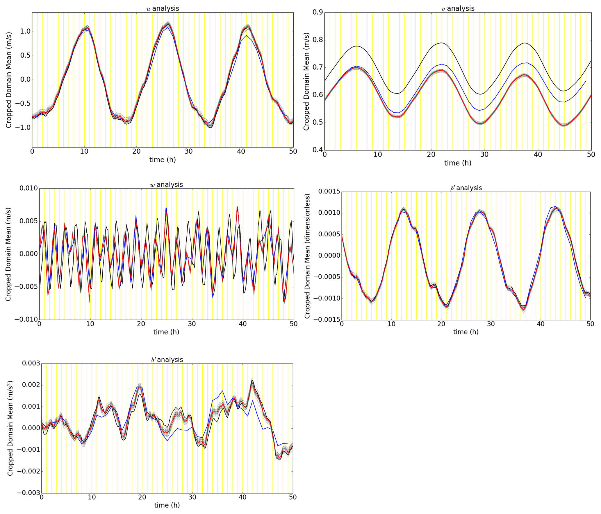
Figure 6 EBV(d) (100 % B_e) ensemble trajectories derived from grid point-averaged analysis fields and their forecasts over a subset of the full domain (a box located at the centre of the domain, model levels 25 to 35, longitudinal grid points 127 to 237). The corresponding ensemble mean (red), free background (blue), and “truth” (black) trajectories for the same subset domain are plotted alongside the individual ensemble member (grey) trajectories. Values for the free background are indicated every hour and every 10 m for the other trajectories.

In Fig. 6, the spread of the EBV(d) ensemble is centred around the ensemble mean throughout the 50 cycles. The “truth” trajectory is also generally contained within the spread of the ensemble, particularly for u, ${\stackrel{\mathrm{̃}}{\mathit{\rho }}}^{\prime }$, and b^′. There was no evidence of filter collapse nor bimodalities which indicates that the DA-centred ensemble generated using the EBV method is healthy.

It is common practice to also compare the ensemble spread with the RMSE which, for a perfectly reliable large ensemble where observation density and errors are accounted for, the two quantities should be approximately the same (Leutbecher, 2009). In the EBV method, the ensemble spread is largely dependent on the choice of ϵ₀ since it does not account for the observation network, but this method is still worth considering as a “control method” and comparing with future methods consistent with Kalman filter theory. In the computation of the ensemble spread, Fortin et al. (2014) also cautions against using the wrong metric. Following their recommended approach, we define the grid point-averaged ensemble spread $\stackrel{\mathrm{‾}}{S_t}$ using the square root grid point-averaged ensemble variance:

$$\begin{array}{}\text{(18)}& \stackrel{\mathrm{‾}}{S_t}=\sqrt{{\displaystyle \frac{\mathrm{1}}{N_{\mathrm{g}}}}\sum _{i=\mathrm{1}}^{N_{\mathrm{g}}}{S}^{\mathrm{2}}[i,t]},\end{array}$$

where the ensemble spread S is computed using Eq. (4) of Whitaker and Loughe (1998). N_g in this case refers to the number of grid points over which the average is taken (i.e. the points within the same box used for Fig. 6) and i is the grid point index which represents points in the box. The RMSE is computed as before except now over points within this box.

Figure 7 shows $\stackrel{\mathrm{‾}}{S_t}$ for each model quantity in the EBV(d) ensemble. These are benchmarked against the RMSE and the (time-stationary) implied background error standard deviations at model level 30 of B_c which are also plotted. For u and ${\stackrel{\mathrm{̃}}{\mathit{\rho }}}^{\prime }$, the ensemble spread approximately matches the RMSE particularly for later cycles as the hybrid control analysis converges around the “truth”. For v, w, and b^′, the ensemble is clearly under-dispersive. For all variables, the ensemble spread is also much smaller than the corresponding implied background error standard deviation at model level 30 of B_c. This strongly suggests that the issue with v analysis errors highlighted in the previous section is due to lack of tuning of the variances of B_c which depends on the specific data assimilation set-up. Note that the ensemble spread is computed with respect to the ensemble mean (Whitaker and Loughe, 1998) but the RMSE is computed between the hybrid control analysis (a surrogate to the ensemble mean) and the “truth”. The spread–error relationship from this set-up suggests that the DA-centring did not result in major statistical inconsistencies with the EBV ensemble. While the spread–error relationship is a useful diagnostic, it is not so straightforward to directly relate the ensemble spread to the eventual skill of the hybrid-EnVar DA system. Hence, it is not easy to determine whether to further inflate or deflate the EBV analysis perturbations by considering other choices of ϵ₀.

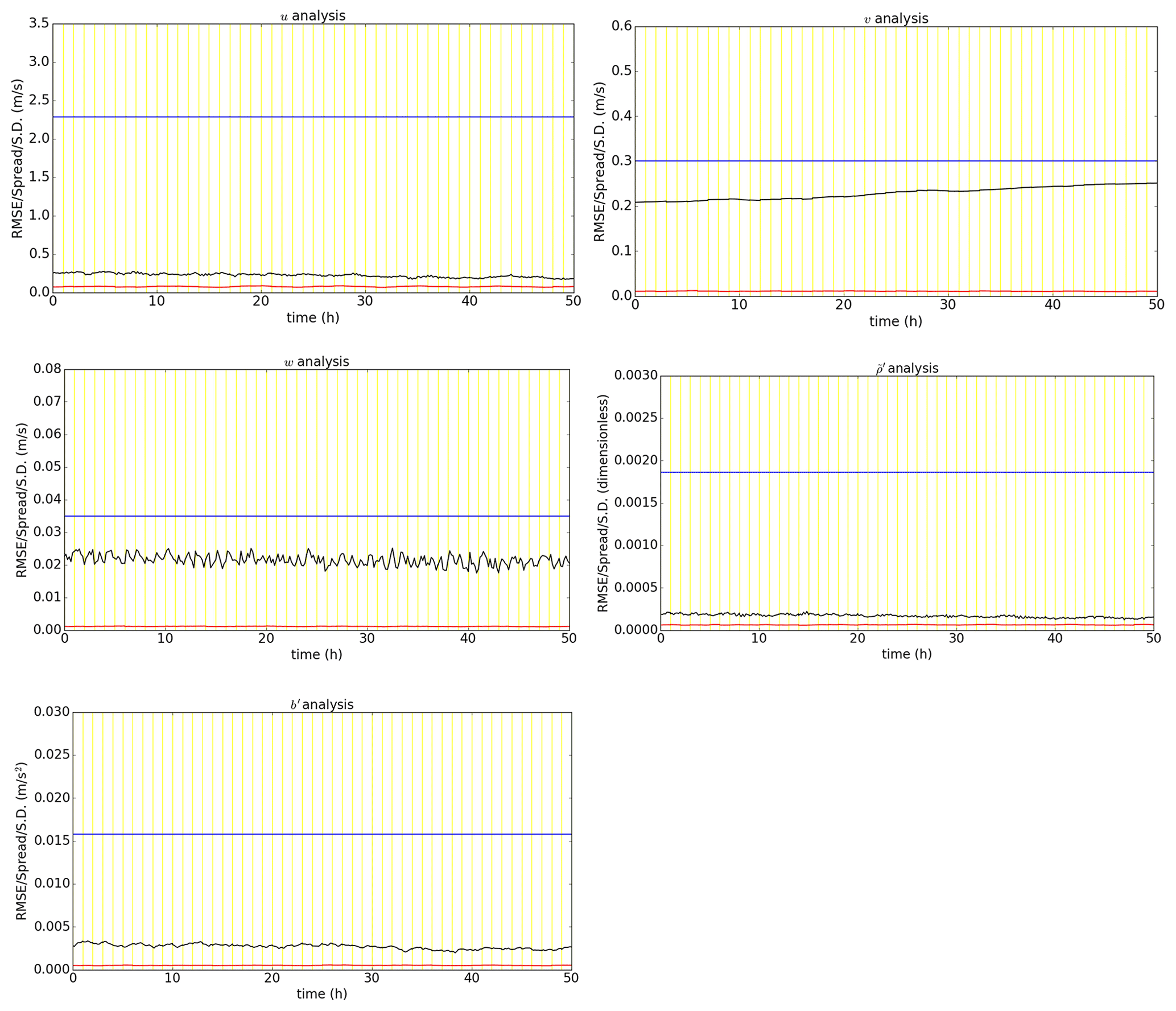
Figure 7 Time series of root mean square analysis errors (black) and ensemble spread (red) for the EBV(d) (100 % B_e) ensemble, computed over a subset of the domain (a box located at the centre of the domain, model levels 25 to 35, longitudinal grid points 127 to 237). The implied (time-stationary) background error standard deviation at model level 30 is also included (blue).

4.5 Sensitivity to number of ensemble members

As mentioned in Sect. 3.2.1, having a finite number of ensemble members will lead to sampling error in ${\mathbf{P}}_{\mathrm{e}}^{\mathrm{f}}\left[t\right]$. Logically, decreasing the number of ensemble members N used to compute ${\mathbf{P}}_{\mathrm{e}}^{\mathrm{f}}\left[t\right]$ should result in larger sampling errors. For a fixed L, we demonstrate the sensitivity of the skill of the hybrid-EnVar DA system to N in the ABC-DA system. We perform two additional experiments as variants of EBV(d) to maximise the impact of the ensemble size changes. The experiments follow the same configuration as EBV(d) but with only 20 and 10 ensemble members in the ensemble instead, referred to as EBV(d20) and EBV(d10), respectively, instead of the 30 members used until now.

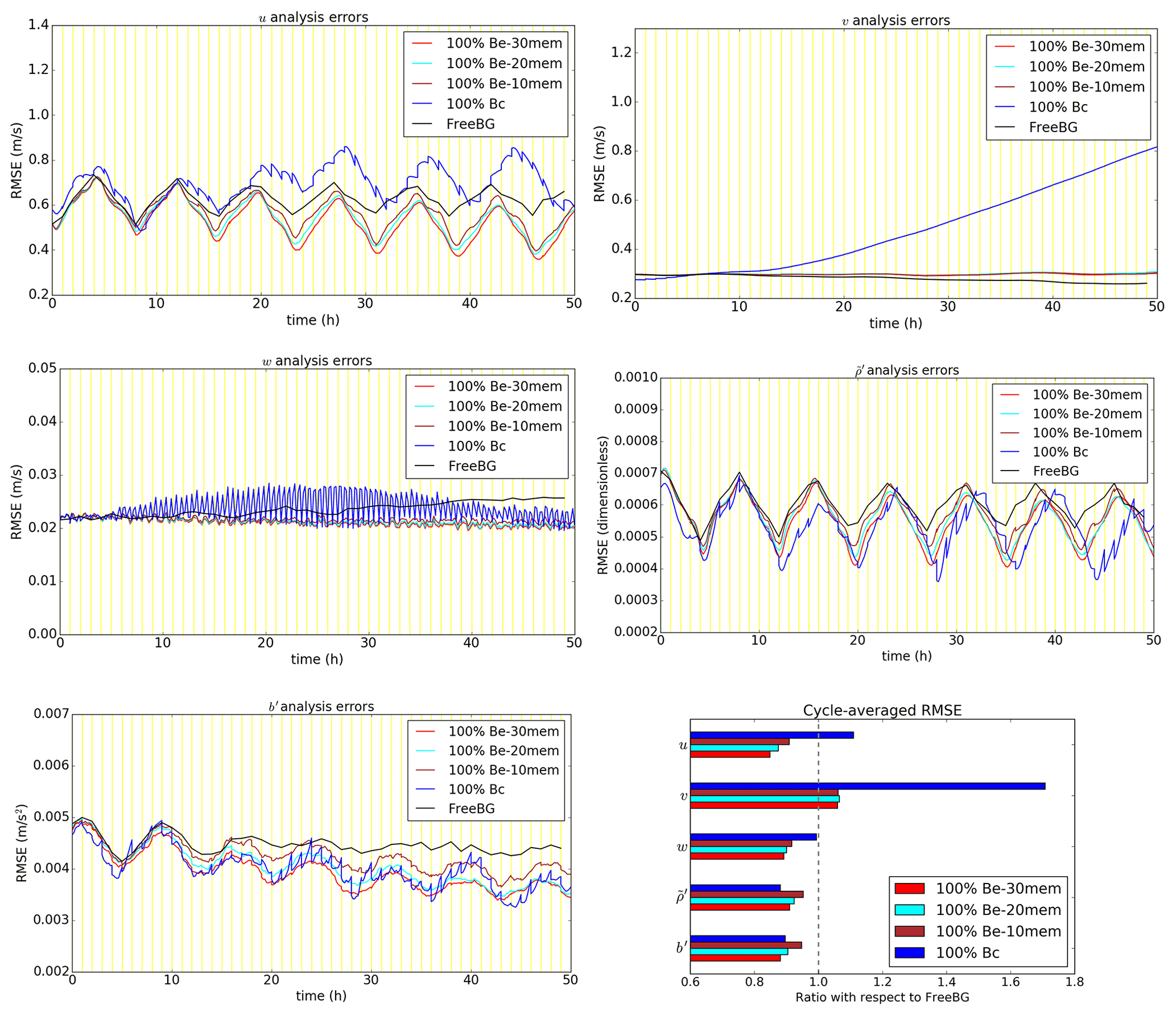
Figure 8 As in Fig. 5, but for EBV(d), EBV(d20), and EBV(d10) experiments (100 % B_e with 30, 20, and 10 ensemble members, respectively).

Figure 8 shows the comparison of cycle-averaged analysis errors as N is varied. The RMSE is smallest in EBV(d) for almost all prognostic variables. Reducing the ensemble size from 30 to 20 in EBV(d20) leads to an increase in the RMSE, indicating poorer performance of the ABC-DA system. A further reduction of the ensemble size to 10 in EBV(d10) leads to the poorest performance overall. In this simple setup, these results are expected following the above argument that larger sampling errors are introduced into the system when N is smaller. For ${\stackrel{\mathrm{̃}}{\mathit{\rho }}}^{\prime }$ and b^′, the RMSE ratio in EBV(d10) is even larger than in EBV(a), indicating that the pure EnVar setup may perform poorer than its 3DVar-FGAT counterpart when the ensemble size is too small (Fig. 8; bottom right panel).

It is important to highlight that the results are specific to this ABC-DA setup where the localisation length-scales are kept fixed (and are arguably quite tight) across the experiments. For other setups where the localisation length-scales are broader, the optimal ensemble size would be expected to be larger. It would also be worth exploring if a further increase in the ensemble size by orders of magnitude would yield a “saturation point” where there is little additional benefit to the system. However, one should also be aware of ensemble clustering (Amezcua et al., 2012) in very large ensembles. This issue has been shown to negatively impact hybrid-EnVar DA in simpler models such as the three variable Lorenz-63 model (Goodliff et al., 2015). In the case of the much larger ABC-DA system though, it is unlikely that N could practically be made large enough relative to n to be exposed to this handicap.

5 Summary

In this article, we document the development of the hybrid ensemble-variational data assimilation system for the ABC model (Petrie et al., 2017) built on the existing variational ABC-DA system (Bannister, 2020). The hybrid ensemble-variational algorithm that is introduced is based on the alpha control variable approach of Lorenc (2003). Key details related to the spatial and inter-variable localisation are discussed; the approach coded in the ABC-DA system allows flexibility in the localisation for use in future exploratory studies. The hybrid ensemble-variational algorithm requires an ensemble system that is run parallel to the deterministic components to provide the flow-dependent error modes. To achieve this, the random field perturbations method is introduced in the ABC model for generating an initial ensemble. The ensemble bred vectors (EBV) method is also introduced in the ABC-DA system to propagate the ensemble, which is centred on the hybrid control analysis at each cycle.

Using a tropical setting of the ABC model, we test both ensemble propagation methods (30-member ensemble) in a series of hourly-cycling multi-cycle data assimilation observation system simulation experiments with hybrid ensemble-variational data assimilation. In the experiments, 3DVar-FGAT (First Guess at Appropriate Time) is employed together with EBV using different weightings assigned to the implied climatological (or static) background error covariance matrix (B_c) and the implied ensemble-derived background error covariance matrix (B_e); (a) 100 % B_c (i.e. no flow-dependency, equivalent to 3DVar-FGAT), (b) 50 % B_c, 50 % B_e; hybrid-En3DVar-FGAT (i.e. flow-dependency with an equal contribution from B_c and B_e), (c) 20 % B_c, 80 % B_e; hybrid-En3DVar-FGAT (i.e. flow-dependency with most contribution from B_e), and (d) 100 % B_e; pure En3DVar-FGAT (i.e. no contribution from B_c).

The cycle-averaged analysis root mean square errors with respect to the “truth” for all prognostic variables except v were generally smaller for the EBV experiments compared to the free background. All experiments that involved the ensemble outperformed pure B_c for all variables. EBV(c) was the best performing configuration for w, ${\stackrel{\mathrm{̃}}{\mathit{\rho }}}^{\prime }$, and b^′ while EBV(d) was the best performing configuration for u and v. We also noted that the v field gradually diverged from the “truth” during the simulations for experiments involving B_c even though fields of other variables were converging around the “truth” as logically expected. Through further assessment of the implied background error covariances and sensitivity tests, it was found that for the tropical setting of the ABC model, there exists some mass–wind relationship that is captured in B_e which is not well-represented by the (weak) geostrophic balance constraint in B_c. We speculate that the issue with v for configurations that involve B_c could be due to the absence of a suitable balance constraint for prescribing the mass–wind relationship which may exist in the tropical setting of the ABC model, warranting further investigation in a separate study since it is not trivial to derive one. The results demonstrate the advantages of employing hybrid ensemble-variational data assimilation in the ABC-DA system over traditional variational data assimilation.

An inspection of the EBV(d) ensemble trajectories showed that the ensemble was centred around the ensemble mean throughout the experiment with the “truth” trajectory generally contained within the spread of the ensemble. For v, w, and b^′, the EBV ensemble was under-dispersive but for u and ${\stackrel{\mathrm{̃}}{\mathit{\rho }}}^{\prime }$, the ensemble spread approximately matched the corresponding RMSE. The EBV ensemble did not exhibit bimodalities or evidence of filter collapse, indicating that the DA-centred ensemble generated was healthy.

To illustrate the sensitivity to ensemble members, we performed two additional experiments as variants of EBV(d); EBV(d20) with 20 ensemble members and EBV(d10) with 10 ensemble members. The cycle-averaged analysis errors for almost all prognostic variables were smallest in EBV(d). Reducing the ensemble size from 30 to 20 and subsequently to 10 led to an increase in the RMSE, indicating poorer performance of the ABC-DA system. The results in this simple setup are consistent with the expectation that larger sampling errors are introduced into the system with a smaller ensemble, thus resulting in larger RMSE.

During the testing and development of the hybrid ensemble-variational method, localisation-related issues like hydrostatic imbalance in the analysis increments also became apparent. Similar issues have been documented in previous studies but we have included additional comments in this article. Given the rapid adoption and broad shift towards hybrid ensemble-variational methods in convective-scale numerical weather prediction, we hope that the ABC-DA system can prove useful in providing further insights and highlight other potential issues that may arise in such methods. Particularly for the tropics, further work is required to better understand the characteristics of the ensemble-derived background errors such as disentangling its flow-dependency or designing the localisation to isolate or identify important multi-variate relationships.

Appendix A: Details on the random field perturbations method

From Sect. 3.1, the random field perturbations method is used to generate the initial ensemble states for the ABC ensemble system. Equation (7) describes the implementation where pairs of states are randomly chosen from a long “truth” run.

In Magnusson et al. (2009), there are additional constraints placed on the choice of random fields. The dates must be from different years and must be from the same season in order to eliminate inter-annual correlations in the perturbations yet preserve the seasonal characteristics of the variability. In the ABC model, we have attempted to capture the essence of these constraints even though there are no seasons in the ABC model.

For the experiments, the long “truth” run is generated with the initial control state ${\mathit{x}}_{\mathrm{cs}}^{\mathrm{c}}$ as the initial condition and is run for 50 d. ABC model dumps are produced every hour, resulting in a total of 1200 state dumps. A minimum threshold of 100 h is set between the validity time of each random pair of states for which they are assumed to be uncorrelated. In other words, pairs of states are selected randomly and are retained only if they are valid at least 100 h apart. Additionally, Magnusson et al. (2009) did not indicate if the dates can be repeatedly selected (i.e. selection from a pool with replacement) so we have not imposed the additional constraint of selection from a pool without replacement. For the experiments, a total of 1200 state dumps is sufficiently large compared to the number of pairs required (number of ensemble members, 30 in most of this work).

One aspect that was highlighted in the implementation was the choice of fixed perturbation amplitude to scale the random field perturbations. It is not possible to follow the exact approach of Magnusson et al. (2009) using the average analysis error statistics in the ABC model. However, we use the same metric (total energy norm) to gauge the initial fixed perturbation amplitude. As described in Sect. 3.1, the random field perturbations are scaled towards their mean total energy norm. This approach ensures that the random fields perturbations have the same fixed perturbation amplitude but differ in directions of error growth. Further testing with the ABC model showed that reducing the fixed perturbation amplitude yielded smaller errors in the experiments so a deflation factor of 5 was eventually adopted.

The total energy (E_tot) for the random field perturbations are computed using

$$\begin{array}{}\text{(A1a)}& {\displaystyle }{E}_{\mathrm{tot}}=E_{\mathrm{k}}+E_{\mathrm{b}}+E_{\mathrm{e}}\text{(A1b)}& {\displaystyle }{E}_{\mathrm{k}}=\int {\displaystyle \frac{\stackrel{\mathrm{̃}}{\mathit{\rho }}(u^{\mathrm{2}}+v^{\mathrm{2}}+w^{\mathrm{2}})}{\mathrm{2}}}{\mathit{\rho }}_{\mathrm{0}}\mathit{d}V\text{(A1c)}& {\displaystyle }{E}_{\mathrm{b}}=\int {\displaystyle \frac{\stackrel{\mathrm{̃}}{\mathit{\rho }}{b^{\prime }}^{\mathrm{2}}}{\mathrm{2}{A}^{\mathrm{2}}}}{\mathit{\rho }}_{\mathrm{0}}\mathit{d}V\text{(A1d)}& {\displaystyle }{E}_{\mathrm{e}}=\int {\displaystyle \frac{C{{\stackrel{\mathrm{̃}}{\mathit{\rho }}}^{\prime }}^{\mathrm{2}}}{\mathrm{2}B}}{\mathit{\rho }}_{\mathrm{0}}\mathit{d}V,\end{array}$$

where E_k, E_b, and E_e are the kinetic, buoyant, and elastic energy, respectively, ρ₀=1.225 kg m⁻³ is a reference air density, and dV is the volume of a grid box in the ABC model. Note that as mentioned in Sect. 3.3.1, we also use $\sqrt{E_{\mathrm{tot}}}$ in the ensemble bred vectors method to scale the ensemble perturbations for subsequent cycles. Prior to the experiments, we performed some initial testing using the inner product norm instead of $\sqrt{E_{\mathrm{tot}}}$ which yielded similar results between the two norm choices. Since $\sqrt{E_{\mathrm{tot}}}$ is a metric that is physically meaningful, it was eventually used for the scaling of the random field perturbations and ensemble perturbations from the ensemble bred vectors method for the experiments.

Appendix B: Accounting for inter-variable covariances – proof of equivalence of two approaches

As highlighted in Sect. 3.2.2, L (the localisation matrix) can be partitioned into a matrix U^α:

$$\begin{array}{}\text{(B1)}& \mathbf{L}={\mathbf{U}}^{\mathit{\alpha }}{\mathbf{U}}^{\mathit{\alpha }\top }.\end{array}$$

We seek to prove that two approaches used to code χ^αk and U^α (described below) give the same result when L is applied on the same model space vector v (of length N_gN_var). Note that L is N_gN_var×N_gN_var which, in principle, means that the inter-variable localisation matrix can be set to have any correlation structure, including the limiting cases of full localisation between different variables (where the corresponding matrix elements are 0) and no localisation (matrix elements are 1). Recall that L is used in the DA via a Schur product with ${\mathbf{P}}_{\mathrm{e}}^{\mathrm{f}}\left[t\right]$ (Eq. 11). While the number of rows in U^α is constrained to be N_gN_var, the number of columns can be chosen. The fewer the columns, the smaller the corresponding size of the χ^αk vectors (Eq. 14b) but the less flexible the implied localisation matrix. The first approach considered is based on Wang et al. (2008a) (N_g columns) and the second approach is coded in the ABC-DA system (N_gN_var columns) inspired by Bannister (2017). The first approach requires less memory and computation but has less flexibility than the second approach in terms of multi-variate localisation choices.

For simplicity, the proof is demonstrated using pure EnVar with one non-zero element in v. This is a similar procedure to computing a column of the implied B_c or B_e but now the implied L is being probed. It is easier to visualise the interactions of the matrix elements by partitioning v into segments of size N_g×1 based on the ABC prognostic variables, i.e. $\mathbf{v}=({\mathbf{v}}_u,{\mathbf{v}}_v,{\mathbf{v}}_w,{\mathbf{v}}_{{\stackrel{\mathrm{̃}}{\mathit{\rho }}}^{\prime }},{\mathbf{v}}_{b^{\prime }}{)}^{\top }$. Similarly, we can consider blocks, each of size N_g×N_g, used to construct U^α (i.e. ${\mathbf{U}}_u^{\mathit{\alpha }},{\mathbf{U}}_v^{\mathit{\alpha }},{\mathbf{U}}_w^{\mathit{\alpha }},{\mathbf{U}}_{{\stackrel{\mathrm{̃}}{\mathit{\rho }}}^{\prime }}^{\mathit{\alpha }},$ and ${\mathbf{U}}_{b^{\prime }}^{\mathit{\alpha }}$) which will determine the spatial localisations (horizontal and vertical) for each variable.

The main difference between the two approaches is in the design of U^α. In the first approach, based on Wang et al. (2008a), U^α (denoted ${\stackrel{\mathrm{̃}}{\mathbf{U}}}^{\mathit{\alpha }}$) is rectangular (N_gN_var×N_g and χ^αk has N_g elements), given by

$$\begin{array}{}\text{(B2)}& {\stackrel{\mathrm{̃}}{\mathbf{U}}}^{\mathit{\alpha }}=\left[\begin{array}{c}{\mathbf{U}}_u^{\mathit{\alpha }}\\ {\mathbf{U}}_v^{\mathit{\alpha }}\\ {\mathbf{U}}_w^{\mathit{\alpha }}\\ {\mathbf{U}}_{{\stackrel{\mathrm{̃}}{\mathit{\rho }}}^{\prime }}^{\mathit{\alpha }}\\ {\mathbf{U}}_{b^{\prime }}^{\mathit{\alpha }}\end{array}\right].\end{array}$$

Applying L (denoted $\stackrel{\mathrm{̃}}{\mathbf{L}}$ for first approach) to v yields

$$\begin{array}{}\text{(B3a)}& \stackrel{\mathrm{̃}}{\mathbf{L}}\mathbf{v}={\stackrel{\mathrm{̃}}{\mathbf{U}}}^{\mathit{\alpha }}{\stackrel{\mathrm{̃}}{\mathbf{U}}}^{\mathit{\alpha }\top }\mathbf{v}=\left[\begin{array}{c}{\mathbf{U}}_u^{\mathit{\alpha }}\\ {\mathbf{U}}_v^{\mathit{\alpha }}\\ {\mathbf{U}}_w^{\mathit{\alpha }}\\ {\mathbf{U}}_{{\stackrel{\mathrm{̃}}{\mathit{\rho }}}^{\prime }}^{\mathit{\alpha }}\\ {\mathbf{U}}_{b^{\prime }}^{\mathit{\alpha }}\end{array}\right]\left[\begin{array}{ccccc}{\mathbf{U}}_u^{\mathit{\alpha }\top }& {\mathbf{U}}_v^{\mathit{\alpha }\top }& {\mathbf{U}}_w^{\mathit{\alpha }\top }& {\mathbf{U}}_{{\stackrel{\mathrm{̃}}{\mathit{\rho }}}^{\prime }}^{\mathit{\alpha }\top }& {\mathbf{U}}_{b^{\prime }}^{\mathit{\alpha }\top }\end{array}\right]\mathbf{v}\end{array}$$

with the elements given by

$$\begin{array}{}\text{(B3b)}& (\stackrel{\mathrm{̃}}{\mathbf{L}}\mathbf{v}{)}_i=\sum _{j=\mathrm{1}}^{N_{\mathrm{g}}}\left\{\left({\stackrel{\mathrm{̃}}{\mathbf{U}}}^{\mathit{\alpha }}{)}_{i,j}\sum _{i^{\prime }=\mathrm{1}}^{N_{\mathrm{g}}{N}_{\mathrm{var}}}\right({\stackrel{\mathrm{̃}}{\mathbf{U}}}^{\mathit{\alpha }\top }{)}_{j,i^{\prime }}{\mathbf{v}}_{i^{\prime }}\right\}.\end{array}$$

If there is only one non-zero element (the qth element of v), this simplifies to

$$\begin{array}{}\text{(B3c)}& \begin{array}{rl}(\stackrel{\mathrm{̃}}{\mathbf{L}}\mathbf{v}{)}_i& =\sum _{j=\mathrm{1}}^{N_{\mathrm{g}}}\left({\stackrel{\mathrm{̃}}{\mathbf{U}}}^{\mathit{\alpha }}{)}_{i,j}\right({\stackrel{\mathrm{̃}}{\mathbf{U}}}^{\mathit{\alpha }\top }{)}_{j,q}\\ & {\mathbf{v}}_q=\sum _{j=\mathrm{1}}^{N_{\mathrm{g}}}\left({\stackrel{\mathrm{̃}}{\mathbf{U}}}^{\mathit{\alpha }}{)}_{i,j}\right({\stackrel{\mathrm{̃}}{\mathbf{U}}}^{\mathit{\alpha }}{)}_{q,j}{\mathbf{v}}_q.\end{array}\end{array}$$

In the second approach, U^α (denoted ${\widehat{\mathbf{U}}}^{\mathit{\alpha }}$) is square (N_gN_var×N_gN_var and χ^αk has N_gN_var elements), given by

$$\begin{array}{}\text{(B4)}& {\widehat{\mathbf{U}}}^{\mathit{\alpha }}=\left[\begin{array}{ccccc}{\mathbf{U}}_u^{\mathit{\alpha }}& \mathbf{0}& \mathbf{0}& \mathbf{0}& \mathbf{0}\\ \mathbf{0}& {\mathbf{U}}_v^{\mathit{\alpha }}& \mathbf{0}& \mathbf{0}& \mathbf{0}\\ \mathbf{0}& \mathbf{0}& {\mathbf{U}}_w^{\mathit{\alpha }}& \mathbf{0}& \mathbf{0}\\ \mathbf{0}& \mathbf{0}& \mathbf{0}& {\mathbf{U}}_{{\stackrel{\mathrm{̃}}{\mathit{\rho }}}^{\prime }}^{\mathit{\alpha }}& \mathbf{0}\\ \mathbf{0}& \mathbf{0}& \mathbf{0}& \mathbf{0}& {\mathbf{U}}_{b^{\prime }}^{\mathit{\alpha }},\end{array}\right]\end{array}$$

where 0 is a N_g×N_g block containing zeroes. This is the default configuration that is coded in the ABC-DA system which gives an implied L (denoted $\widehat{\mathbf{L}}$ for the second approach):

$$\begin{array}{}\text{(B5)}& \widehat{\mathbf{L}}={\widehat{\mathbf{U}}}^{\mathit{\alpha }}{\widehat{\mathbf{U}}}^{\mathit{\alpha }\top }=\left[\begin{array}{ccccc}{\mathbf{U}}_u^{\mathit{\alpha }}{\mathbf{U}}_u^{\mathit{\alpha }\top }& \mathbf{0}& \mathbf{0}& \mathbf{0}& \mathbf{0}\\ \mathbf{0}& {\mathbf{U}}_v^{\mathit{\alpha }}{\mathbf{U}}_v^{\mathit{\alpha }\top }& \mathbf{0}& \mathbf{0}& \mathbf{0}\\ \mathbf{0}& \mathbf{0}& {\mathbf{U}}_w^{\mathit{\alpha }}{\mathbf{U}}_w^{\mathit{\alpha }\top }& \mathbf{0}& \mathbf{0}\\ \mathbf{0}& \mathbf{0}& \mathbf{0}& {\mathbf{U}}_{{\stackrel{\mathrm{̃}}{\mathit{\rho }}}^{\prime }}^{\mathit{\alpha }}{\mathbf{U}}_{{\stackrel{\mathrm{̃}}{\mathit{\rho }}}^{\prime }}^{\mathit{\alpha }\top }& \mathbf{0}\\ \mathbf{0}& \mathbf{0}& \mathbf{0}& \mathbf{0}& {\mathbf{U}}_{b^{\prime }}^{\mathit{\alpha }}{\mathbf{U}}_{b^{\prime }}^{\mathit{\alpha }\top }\end{array}\right]\end{array}$$

Notice that here, $\widehat{\mathbf{L}}$ does a full inter-variable localisation so that the Schur product of $\widehat{\mathbf{L}}$ with ${\mathbf{P}}_{\mathrm{e}}^{\mathrm{f}}\left[t\right]$ will not retain any inter-variable covariances. This may be useful if N is small and sampling noise is problematic in ${\mathbf{P}}_{\mathrm{e}}^{\mathrm{f}}\left[t\right]$.

Next, we introduce a mapping matrix $\widehat{\mathbf{I}}$ which consists of N_p×N_p blocks of identity matrices (${\mathbf{I}}_{N_{\mathrm{g}}}$, each of size N_g×N_g):

$$\begin{array}{}\text{(B6)}& \widehat{\mathbf{I}}={\displaystyle \frac{\mathrm{1}}{\sqrt{N_{\mathrm{p}}}}}\left[\begin{array}{ccccc}{\mathbf{I}}_{N_{\mathrm{g}}}& {\mathbf{I}}_{N_{\mathrm{g}}}& {\mathbf{I}}_{N_{\mathrm{g}}}& {\mathbf{I}}_{N_{\mathrm{g}}}& {\mathbf{I}}_{N_{\mathrm{g}}}\\ {\mathbf{I}}_{N_{\mathrm{g}}}& {\mathbf{I}}_{N_{\mathrm{g}}}& {\mathbf{I}}_{N_{\mathrm{g}}}& {\mathbf{I}}_{N_{\mathrm{g}}}& {\mathbf{I}}_{N_{\mathrm{g}}}\\ {\mathbf{I}}_{N_{\mathrm{g}}}& {\mathbf{I}}_{N_{\mathrm{g}}}& {\mathbf{I}}_{N_{\mathrm{g}}}& {\mathbf{I}}_{N_{\mathrm{g}}}& {\mathbf{I}}_{N_{\mathrm{g}}}\\ {\mathbf{I}}_{N_{\mathrm{g}}}& {\mathbf{I}}_{N_{\mathrm{g}}}& {\mathbf{I}}_{N_{\mathrm{g}}}& {\mathbf{I}}_{N_{\mathrm{g}}}& {\mathbf{I}}_{N_{\mathrm{g}}}\\ {\mathbf{I}}_{N_{\mathrm{g}}}& {\mathbf{I}}_{N_{\mathrm{g}}}& {\mathbf{I}}_{N_{\mathrm{g}}}& {\mathbf{I}}_{N_{\mathrm{g}}}& {\mathbf{I}}_{N_{\mathrm{g}}}\end{array}\right],\end{array}$$

where N_p is the number of model variables whose inter-variable covariances are retained by the mapping matrix (i.e. $N_{\mathrm{p}}=N_{\mathrm{var}}=\mathrm{5}$ in the above). Note that other designs of $\widehat{\mathbf{I}}$ (e.g. replacing some blocks with 0) will allow only the desired retention of specific covariances between certain model variables.

Using the second approach of coding U^α and χ^αk, it is possible to retain the full inter-variable covariances and achieve the exact same outcome as the first approach by defining ${\mathbf{U}}^{\mathit{\alpha }}={\widehat{\mathbf{U}}}^{\mathit{\alpha }}\widehat{\mathbf{I}}$. The implied localisation matrix is thus $\mathbf{L}=\frac{\mathrm{1}}{N_{\mathrm{p}}}{\widehat{\mathbf{U}}}^{\mathit{\alpha }}\widehat{\mathbf{I}}\widehat{\mathbf{I}}{\widehat{\mathbf{U}}}^{\mathit{\alpha }\top }$. As before, applying L to v yields

$$\begin{array}{}\text{(B7a)}& \begin{array}{rl}\mathbf{Lv}& ={\displaystyle \frac{\mathrm{1}}{N_{\mathrm{p}}}}{\widehat{\mathbf{U}}}^{\mathit{\alpha }}\widehat{\mathbf{I}}\widehat{\mathbf{I}}{\widehat{\mathbf{U}}}^{\mathit{\alpha }\top }\mathbf{v}={\displaystyle \frac{\mathrm{1}}{N_{\mathrm{p}}}}\left[\begin{array}{ccccc}{\mathbf{U}}_u^{\mathit{\alpha }}& {\mathbf{U}}_u^{\mathit{\alpha }}& {\mathbf{U}}_u^{\mathit{\alpha }}& {\mathbf{U}}_u^{\mathit{\alpha }}& {\mathbf{U}}_u^{\mathit{\alpha }}\\ {\mathbf{U}}_v^{\mathit{\alpha }}& {\mathbf{U}}_v^{\mathit{\alpha }}& {\mathbf{U}}_v^{\mathit{\alpha }}& {\mathbf{U}}_v^{\mathit{\alpha }}& {\mathbf{U}}_v^{\mathit{\alpha }}\\ {\mathbf{U}}_w^{\mathit{\alpha }}& {\mathbf{U}}_w^{\mathit{\alpha }}& {\mathbf{U}}_w^{\mathit{\alpha }}& {\mathbf{U}}_w^{\mathit{\alpha }}& {\mathbf{U}}_w^{\mathit{\alpha }}\\ {\mathbf{U}}_{{\stackrel{\mathrm{̃}}{\mathit{\rho }}}^{\prime }}^{\mathit{\alpha }}& {\mathbf{U}}_{{\stackrel{\mathrm{̃}}{\mathit{\rho }}}^{\prime }}^{\mathit{\alpha }}& {\mathbf{U}}_{{\stackrel{\mathrm{̃}}{\mathit{\rho }}}^{\prime }}^{\mathit{\alpha }}& {\mathbf{U}}_{{\stackrel{\mathrm{̃}}{\mathit{\rho }}}^{\prime }}^{\mathit{\alpha }}& {\mathbf{U}}_{{\stackrel{\mathrm{̃}}{\mathit{\rho }}}^{\prime }}^{\mathit{\alpha }}\\ {\mathbf{U}}_{b^{\prime }}^{\mathit{\alpha }}& {\mathbf{U}}_{b^{\prime }}^{\mathit{\alpha }}& {\mathbf{U}}_{b^{\prime }}^{\mathit{\alpha }}& {\mathbf{U}}_{b^{\prime }}^{\mathit{\alpha }}& {\mathbf{U}}_{b^{\prime }}^{\mathit{\alpha }}\end{array}\right]\\ & \left[\begin{array}{ccccc}{\mathbf{U}}_u^{\mathit{\alpha }\top }& {\mathbf{U}}_v^{\mathit{\alpha }\top }& {\mathbf{U}}_w^{\mathit{\alpha }\top }& {\mathbf{U}}_{{\stackrel{\mathrm{̃}}{\mathit{\rho }}}^{\prime }}^{\mathit{\alpha }\top }& {\mathbf{U}}_{b^{\prime }}^{\mathit{\alpha }\top }\\ {\mathbf{U}}_u^{\mathit{\alpha }\top }& {\mathbf{U}}_v^{\mathit{\alpha }\top }& {\mathbf{U}}_w^{\mathit{\alpha }\top }& {\mathbf{U}}_{{\stackrel{\mathrm{̃}}{\mathit{\rho }}}^{\prime }}^{\mathit{\alpha }\top }& {\mathbf{U}}_{b^{\prime }}^{\mathit{\alpha }\top }\\ {\mathbf{U}}_u^{\mathit{\alpha }\top }& {\mathbf{U}}_v^{\mathit{\alpha }\top }& {\mathbf{U}}_w^{\mathit{\alpha }\top }& {\mathbf{U}}_{{\stackrel{\mathrm{̃}}{\mathit{\rho }}}^{\prime }}^{\mathit{\alpha }\top }& {\mathbf{U}}_{b^{\prime }}^{\mathit{\alpha }\top }\\ {\mathbf{U}}_u^{\mathit{\alpha }\top }& {\mathbf{U}}_v^{\mathit{\alpha }\top }& {\mathbf{U}}_w^{\mathit{\alpha }\top }& {\mathbf{U}}_{{\stackrel{\mathrm{̃}}{\mathit{\rho }}}^{\prime }}^{\mathit{\alpha }\top }& {\mathbf{U}}_{b^{\prime }}^{\mathit{\alpha }\top }\\ {\mathbf{U}}_u^{\mathit{\alpha }\top }& {\mathbf{U}}_v^{\mathit{\alpha }\top }& {\mathbf{U}}_w^{\mathit{\alpha }\top }& {\mathbf{U}}_{{\stackrel{\mathrm{̃}}{\mathit{\rho }}}^{\prime }}^{\mathit{\alpha }\top }& {\mathbf{U}}_{b^{\prime }}^{\mathit{\alpha }\top }\end{array}\right]\mathbf{v},\end{array}\end{array}$$

with the elements given by

$$\begin{array}{}\text{(B7b)}& (\mathbf{Lv}{)}_i={\displaystyle \frac{\mathrm{1}}{N_{\mathrm{p}}}}\sum _{j=\mathrm{1}}^{N_{\mathrm{g}}{N}_{\mathrm{p}}}\left\{\left({\mathbf{U}}^{\mathit{\alpha }}{)}_{i,j}\sum _{i^{\prime }=\mathrm{1}}^{N_{\mathrm{g}}{N}_{\mathrm{p}}}\right({\mathbf{U}}^{\mathit{\alpha }\top }{)}_{j,i^{\prime }}{\mathbf{v}}_{i^{\prime }}\right\}.\end{array}$$

Note how in this case, the rows of U^α⊤ are the same as in ${\stackrel{\mathrm{̃}}{\mathbf{U}}}^{\mathit{\alpha }\top }$ from the first approach (Eq. B2) but repeated N_p times. If there is only one non-zero element (the qth element of v), then the computation simplifies to

$$\begin{array}{}\text{(B7c)}& \begin{array}{rl}(\mathbf{Lv}{)}_i& ={\displaystyle \frac{\mathrm{1}}{N_{\mathrm{p}}}}\sum _{j=\mathrm{1}}^{N_{\mathrm{g}}{N}_{\mathrm{p}}}\left({\mathbf{U}}^{\mathit{\alpha }}{)}_{i,j}\right({\mathbf{U}}^{\mathit{\alpha }\top }{)}_{j,q}{\mathbf{v}}_q\\ & ={\displaystyle \frac{\mathrm{1}}{N_{\mathrm{p}}}}\sum _{j=\mathrm{1}}^{N_{\mathrm{g}}}{N}_{\mathrm{p}}\left({\stackrel{\mathrm{̃}}{\mathbf{U}}}^{\mathit{\alpha }}{)}_{i,j}\right({\stackrel{\mathrm{̃}}{\mathbf{U}}}^{\mathit{\alpha }}{)}_{q,j}{\mathbf{v}}_q\\ & =\sum _{j=\mathrm{1}}^{N_{\mathrm{g}}}\left({\stackrel{\mathrm{̃}}{\mathbf{U}}}^{\mathit{\alpha }}{)}_{i,j}\right({\stackrel{\mathrm{̃}}{\mathbf{U}}}^{\mathit{\alpha }}{)}_{q,j}{\mathbf{v}}_q,\end{array}\end{array}$$

noting that when N_p=N_var, full inter-variable covariances are retained. In the computation of any inner products of χ^αk in the variational algorithm, such as for the minimisation or in the computation of J_e, these also have to be scaled by $\frac{\mathrm{1}}{N_{\mathrm{p}}}$ accordingly.

The key thing to note here is that when using both approaches with ${\stackrel{\mathrm{̃}}{\mathbf{U}}}^{\mathit{\alpha }}$ and U^α respectively, the implied localisation matrices are the same ($\stackrel{\mathrm{̃}}{\mathbf{L}}=\mathbf{L}$) as demonstrated by Eqs. (B3c) and (B7c) being the same. Given the greater flexibility, the second approach was coded in the ABC-DA system.

Appendix C: Hydrostatic imbalance due to vertical localisation

According to Eq. (3) of Bannister (2020), the hydrostatic balance relation in the ABC model (also used in the control variable transform) is given by

$$\begin{array}{}\text{(C1)}& C{\displaystyle \frac{\partial {\stackrel{\mathrm{̃}}{\mathit{\rho }}}^{\prime }}{\partial z}}=b^{\prime }.\end{array}$$

From Eq. (1), the prognostic w equation indicates that the change in w following an air parcel (i.e. a Lagrangian frame of reference) is given by the source/sink terms $C\frac{\partial {\stackrel{\mathrm{̃}}{\mathit{\rho }}}^{\prime }}{\partial z}$ and b^′. This neatly corresponds to hydrostatic balance. In other words, hydrostatic imbalance will lead to sources/sinks in w as the system evolves.

Applying vertical localisation directly to the ensemble-derived error modes via the Schur product results in alterations in the vertical gradient of the ${\stackrel{\mathrm{̃}}{\mathit{\rho }}}^{\prime }$ field depending on the kurtosis of the correlation curve applied. We can consider the following scenario: assuming that the ensemble forecasts are hydrostatically balanced on the large scales, one could expect that assimilating a single ${\stackrel{\mathrm{̃}}{\mathit{\rho }}}^{\prime }$ observation without vertical localisation would result in hydrostatically balanced ${\stackrel{\mathrm{̃}}{\mathit{\rho }}}^{\prime }$ and b^′ increments. However, with vertical localisation, the sharpness of the correlation curve superimposes on the ${\stackrel{\mathrm{̃}}{\mathit{\rho }}}^{\prime }$ fields in the ensemble-derived error modes and results in increments that decrease more rapidly with distance (sharper gradient) from the point of observation. Thus, a larger b^′ increment is required in order to maintain hydrostatic balance but the actual b^′ increments are also reduced by the Schur product. In this scenario, the resulting b^′ increments would be sub-hydrostatic.

During the spin-up configuration testing with vertical localisation applied, it was noted that the root mean square value of the w field was gradually increasing throughout the earlier stages of the spin-up process. Since there exists a restoring A²w source term in the prognostic b^′ equation, the root mean square value of the w field does not increase indefinitely because of corresponding induced changes in the b^′ field.