Embedding a one-column ocean model in the Community Atmosphere Model 5.3 to improve Madden–Julian Oscillation simulation in boreal winter

The effect of the air–sea interaction on the Madden–Julian Oscillation (MJO) was investigated using the one-column ocean model Snow–Ice–Thermocline (SIT 1.06) embedded in the Community Atmosphere Model 5.3 (CAM5.3; hereafter CAM5–SIT v1.0). The SIT model with 41 vertical layers was developed to simulate sea surface temperature (SST) and upper-ocean temperature variations with a high vertical resolution that resolves the cool skin and diurnal warm layer and the upper oceanic temperature gradient. A series of 30-year sensitivity experiments were conducted in which various model configurations (e.g., coupled versus uncoupled, vertical resolution and depth of the SIT model, coupling domains, and absence of the diurnal cycle) were considered to evaluate the effect of air–sea coupling on MJO simulation. Most of the CAM5–SIT experiments exhibit higher fidelity than the CAM5-alone experiment in characterizing the basic features of the MJO such as spatiotemporal variability and the eastward propagation in boreal winter. The overall MJO simulation performance of CAM5–SIT benefits from (1) better resolving the fine vertical structure of upper-ocean temperature and therefore the air–sea interaction that results in more realistic intraseasonal variability in both SST and atmospheric circulation and (2) the adequate thickness of a vertically gridded ocean layer. The sensitivity experiments demonstrate the necessity of coupling the tropical eastern Pacific in addition to the tropical Indian Ocean and the tropical western Pacific. Coupling is more essential in the south than north of the Equator in the tropical western Pacific. Enhanced MJO could be obtained without considering the diurnal cycle in coupling.

1 Introduction

The Madden–Julian Oscillation (MJO) is a tropical large-scale convection circulation system that propagates eastward across the warm pool region from the tropical Indian Ocean (IO) to the western Pacific (WP) on an intraseasonal timescale (Madden and Julian, 1972). The MJO is not just an atmospheric phenomenon. The findings from a multination field campaign in the tropics called the Dynamics of MJO/Cooperative Indian Ocean Experiment on Intraseasonal Variability in the Year 2011 (DYNAMO/CINDY2011; de Szoeke et al., 2017; Johnson and Ciesielski, 2017; Pujiana et al., 2018; Yoneyama et al., 2013; Zhang and Yoneyama, 2017) revealed vigorous air–sea coupling during the evolution of the MJO (Chang et al., 2019; DeMott et al., 2015; Jiang et al., 2015, 2020; Kim et al., 2010; Li et al., 2016, 2020; Newman et al., 2009; Pei et al., 2018; Tseng et al., 2014). During the suppression of convection, the MJO propagates eastward with light winds, which is accompanied by enhanced downwelling shortwave radiation absorption, weaker upward latent and sensible fluxes, less cloudiness and precipitation, and weaker vertically turbulent mixing in the upper ocean, thus causing an increase in the upper-ocean temperature. In the following active phase when deep convection occurs, downwelling shortwave radiation is reduced, and stronger westerly winds enhance latent and sensible heat flux (LHF and SHF) loss from the ocean surface, thus causing a decrease in the upper-ocean temperature (DeMott et al., 2015; Madden and Julian, 1972, 1994; Zhang, 2005).

In addition to the tropical ocean surface, the structure of the upper ocean also evolves. Alappattu et al. (2017) reported that during an MJO event, surface flux perturbations cause changes in the ocean thermohaline structure, thus affecting the mixed-layer temperature. The following change in sea surface temperature (SST) can further affect atmospheric circulation of the MJO. Variations in SST mediate LHF and SHF exchange across the air–sea interface. Although SST responds to atmospheric forcing, the modulation of LHF and SHF provides feedback to the atmosphere (DeMott et al., 2015; Jiang et al., 2020). Li et al. (2008, 2020) proposed that the phase relationship between SST and convection implies a delayed air–sea interaction mechanism, whereby a preceding active-phase MJO may trigger an inactive-phase MJO through the delayed effect of the induced SST anomaly over the IO. The reduction in SST caused by a preceding active-phase MJO may, in turn, yield delayed ocean feedback that initiates a suppressed-phase MJO and vice versa. The by-no-means-negligible effect of intraseasonal SST variations caused by surface heat fluxes suggests that the ocean state can affect the MJO (DeMott et al., 2015, 2019; Hong et al., 2017; Li et al., 2020).

Since its discovery almost 5 decades ago, the MJO remains a phenomenon that poses a challenge to the capacity of state-of-the-art atmospheric general circulation models (AGCMs) such as those participating in the Coupled Model Intercomparison Project phase 5 and 6 to generate successful simulations (Ahn et al., 2017, 2020; Bui and Maloney, 2018; Jiang et al., 2020; Hung et al., 2013; Kim et al., 2011).

Recent studies have reported that air–sea coupling improves the representation of the MJO in numerical simulation (Bernie et al., 2008; Crueger et al., 2013; DeMott et al., 2015; Li et al., 2016, 2020; Tseng et al., 2014; Woolnough et al., 2007). Tseng et al. (2014) indicated that effectively resolving the tropical upper-ocean warm layer to capture temperature variations in the upper few meters of the ocean could improve MJO simulation. DeMott et al. (2015) suggested that the tropical atmosphere–ocean interaction may sustain or amplify the pattern of the enhanced and suppressed atmospheric convection of the eastward propagation. DeMott et al. (2019) demonstrated that the improved MJO eastward propagation in four coupled models resulted from enhanced low-level convective moistening for a rainfall rate of >5 mm d⁻¹ due to air–sea coupling. In addition, numerical experiments have been performed to investigate the effect of the diurnal cycle on the MJO (Hagos et al., 2016; Oh et al., 2013), with the results suggesting that the strength and propagation of the MJO through the Maritime Continent (MC) were enhanced when the diurnal cycle was ignored.

Although previous studies have demonstrated the importance of considering the air–sea interaction in a numerical model to improve MJO simulation, additional details regarding model configuration (e.g., vertical resolution and total depth of the vertically gridded ocean, coupling domain, and absence of the diurnal cycle in air–sea coupling) have not been systematically explored. Tseng et al. (2014) coupled the one-column ocean model Snow–Ice–Thermocline (SIT; Tu and Tsuang, 2005) to the fifth generation of the ECHAM AGCM (ECHAM5–SIT) in the tropics and indicated that a vertical resolution of 1 m was essential to yield an improved simulation of the MJO with a realistic strength and eastward propagation speed.

In this study, we coupled the SIT model to the Community Atmosphere Model version 5.3 (CAM5.3; Neale et al., 2012) – the atmosphere component of the Community Earth System Model version 1.2.2 (CESM1.2.2; Hurrell et al., 2013) – to explore the improvement of MJO simulation by coupling the SIT model to another AGCM to be reproducible in modeling science. The CAM5.3, which has been widely used for the long-term simulation of the climate system, could not efficiently simulate the eastward propagation of the MJO; instead, the model simulated a tendency for the MJO to move westward in the IO (Boyle et al., 2015; Jiang et al., 2015). By contrast, the updated CESM2 with the new CAM6 could realistically simulate the MJO (Ahn et al., 2020; Danabasoglu et al., 2020). Thus, the well-explored CAM5, which does not produce a realistic MJO, appears to be a favorable choice for exploring coupling a simple one-dimensional (1-D) ocean model over the tropical oceans, such as the SIT model, and can improve MJO simulation and the effects of model configuration on the degree of the improvement. Such a study can also enhance our understanding regarding the effect of air–sea coupling on the MJO.

The MJO, a tropical atmosphere system that exhibits a more substantial eastward propagation in boreal winter than in other seasons, was the targeted feature in this study. To examine the sensitivity of MJO simulations to different configurations of the tropical air–sea coupling, we conducted a series of 30-year numerical experiments by considering various model configurations (e.g., coupled versus uncoupled, vertical resolution and depth of the SIT model, coupling domains, and absence of the diurnal cycle) to investigate the effect of air–sea coupling. This paper is organized as follows. Section 2 describes the data for validation, the model used for simulation, and the design of numerical experiments. Section 3 describes the effect of various tropical air–sea coupling configurations on the MJO simulation determined through detailed MJO diagnostics. Discussion and conclusions are provided in Sect. 4.

2 Data, methodology, model description, and experimental designs

2.1 Data and methodology

The data analyzed in this study include precipitation from the Global Precipitation Climatology Project (GPCP), outgoing longwave radiation (OLR) and daily SST (Optimum Interpolation SST; OISST) from the National Oceanic and Atmosphere Administration (NOAA), and parameters from the ERA-Interim (ERA-I) reanalysis (Adler et al., 2003; Dee et al., 2011; Lee et al., 2011; Reynolds and Smith, 1995; Schreck et al., 2018). The SST data for the SIT model were obtained from the Hadley Centre Sea Ice and Sea Surface Temperature dataset (Rayner et al., 2003; HadISST1), and the ocean subsurface data (40-layer climatological ocean temperature, salinity, and currents) for nudging were retrieved from the National Centers for Environmental Prediction (NCEP) Global Ocean Data Assimilation System (GODAS; Behringer and Xue, 2004).

We used the CLIVAR MJO Working Group diagnostics package (CLIVAR, 2009) and a 20–100 d filter (Wang et al., 2014) to determine intraseasonal variability. MJO phases were defined following the index (namely, RMM1 and RMM2) proposed by Wheeler and Hendon (2004), which considered the first two principal components of the combined near-equatorial OLR and zonal winds at 850 and 200 hPa. The bandpass-filtered data were used for calculating the index and defining phases.

2.2 Model description

2.2.1 CAM5.3

The CAM5.3 used in this study has a horizontal resolution of 1.9^∘ latitude × 2.5^∘ longitude and 30 vertical levels with the model top at 0.1 hPa. The MJO could not be realistically simulated in the CAM5.3. Boyle et al. (2015) demonstrated that although making the deep convection dependent on SST improved the simulation of the MJO variance, it exerted a significant negative effect on the mean-state climate of low-level cloud and absorbed shortwave radiation. By comparing the simulation results of an uncoupled and coupled CAM5.3, Li et al. (2016) suggested that air–sea coupling and the convection scheme most significantly affected the MJO simulation in the climate model.

2.2.2 1-D high-resolution TKE ocean model

The 1-D high-resolution turbulence kinetic energy (TKE) ocean model SIT was used to simulate the diurnal fluctuation of SST and surface energy fluxes (Lan et al., 2010; Tseng et al., 2014; Tu and Tsuang, 2005). A description of the 1-D high-resolution ocean model SIT can be found in the Appendix. The model was verified well against in situ measurements on board the R/V Oceanographic Research Vessel 1 and 3 over the South China Sea (Lan et al., 2010) and on R/V Vickers over the tropical WP (Tu and Tsuang, 2005).

The SIT model determines the vertical profiles of the temperature and momentum of a water column from the surface down to the seabed, except in the fixed-ocean model bottom experiment. The default setting of vertical discretization (e.g., in the control coupled experiment) is 41 layers, with 12 layers in the first 10.5 m and 6 layers between 10.5 and 107.8 m (Appendix Fig. A1). In the 1-D TKE ocean model, temperature and salinity below 107.8 m, where vertical turbulent mixing is greatly weakened, are nudged toward the climatological values of GODAS data until 4607 m. The extra-high vertical resolution is needed to catch detailed temporal variation of upper ocean temperature, characterized by the warm layer and cool skin (Tu and Tsuang, 2005). To account for the neglected horizontal advection heat flux, the ocean is weakly nudged (using a 30 d timescale) between 10.5 and 107.8 m and strongly nudged (using a 1 d timescale) below 107.8 m according to the NCEP GODAS climatological ocean temperature. No nudging is performed within the uppermost 10.5 m. The SIT model performs calculations twice for each CAM5 time step (30 min; i.e., coupling 48 times per day).

2.3 Experimental design

A series of 30-year numerical experiments (Table 1) were conducted to investigate the effect of the air–sea interaction on the MJO simulation. The HadSST1 used to force the coupled and uncoupled model was the climatological monthly-mean SST averaged over 1982–2001. The monthly SST was linearly interpolated to daily SST fluctuation that forced the model. The SST in the air–sea coupling tropical region was recalculated by the SIT during the simulation, while the prescribed annual cycle of SST was used in the areas outside the coupling region. Ocean bathymetry of the SIT was derived from the NOAA ETOPO1 data (Amante and Eakins, 2009) and interpolated into $\mathrm{1.9}{}^{\circ }\times \mathrm{2.5}{}^{\circ }$ horizontal resolution.

Table 1 List of experiments.

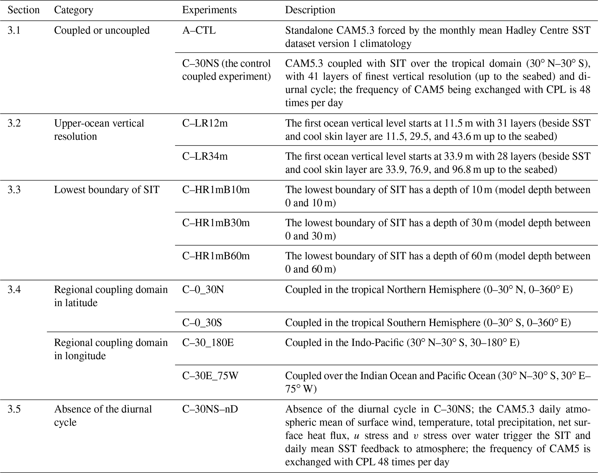
Experiment abbreviations: “A” is the standalone AGCM simulation, and “C” is the CAM5.3 coupled to the SIT model.

All simulations were driven by the prescribed annual cycle of SST repeatedly for 30 years. The strategy is to evaluate the simulation capacity of climate models under the same condition without considering interannual variation induced by SST. This approach has been widely adopted in many studies (Delworth et al., 2006; Haertel, 2020; Subramanian et al., 2011; Tseng et al., 2014; Wang et al., 2005).

Atmospheric initial conditions and external forcing such as CO₂, ozone, and aerosol in near-equilibrium climate state around the year 2000 were taken from the F_2000_CAM5 component set based on CESM1.2.2 framework development. The data have been commonly used in present-day simulations using CAM5 (e.g., He et al., 2017).

The setup of five sets of experiment conducted in this study are described as follows.

1. A standalone CAM5.3 simulation. This was forced by climatological monthly HadISST1 (A–CTL) and the control experiment of coupled CAM5–SIT simulation (C–30NS; 41 vertical levels, coupling in the entire tropics between 30^∘ N and 30^∘ S with a diurnal cycle). The reasons for tropical coupling are twofold. Considering that the MJO is essentially a tropical phenomenon, the coupling was implemented only between 30^∘ N and 30^∘ S. Secondly, coupling a one-dimensional ocean model in the extratropics without surface flux correction as in our case would ignore the impacts of strong ocean currents (such as the Kuroshio and Gulf Stream) and result in large biases.

2. Upper-ocean vertical-resolution experiment. Two simulations with the first layer are centered at 12 m (C–LR12 m) and 34 m (C–LR34m). Further details of the experimental design are shown in Appendix Fig. A1. This experiment demonstrates the significant improvement that a fine vertical resolution can achieve compared to the coarse resolution (e.g., tens of meters) that is often adopted in slab ocean models.

3. Shallow ocean bottom experiment. Three simulations are conducted with the ocean model bottom at 10 m (C–HR1mB10m), 30 m (C–HR1mB30m), and 60 m (C–HR1mB60m) (Appendix Fig. A2). Note that all experiments retained the same vertical resolution (e.g., 1 m in the first top 10 m of the ocean) but with various ocean bottoms (i.e., 10, 30, and 60 m). The purpose is to demonstrate how the total ocean heat content, which depends on the total depth of the ocean, can affect the MJO.

4. Regional coupling experiment. Four simulations are conducted with the coupling region in 0–30^∘ N (C–0_30N) and 0–30^∘ S (C–0_30S) for the latitudinal effect and 30–180^∘ E (C–30_180E) and 30^∘ E–75^∘ W (C–30E_75W) for the longitudinal effect. The coupling domains are shown in Fig. 1. In this experiment we identified the key ocean basins where coupling is essential.

5. Diurnal cycle experiment. To explore the effect of the diurnal coupling cycle, a non-diurnal simulation was conducted for a comparison with the C–30NS simulation. The non-diurnal simulation (C–30NS–nD) considers the air–sea interaction only once a day, namely, calculating SHF and LHF based on daily mean atmospheric variables and SST. To prevent the inconsistent local time in different regions, the coupling frequency at each grid point remained 48 times per day using the same daily means of atmospheric variables and SST at that particular point. In contrast, the control simulation calculates air–sea fluxes 48 times a day based on instantaneous values. A comparison between the non-diurnal simulation and the control simulation reveals the effect of the diurnal cycle in air–sea coupling.

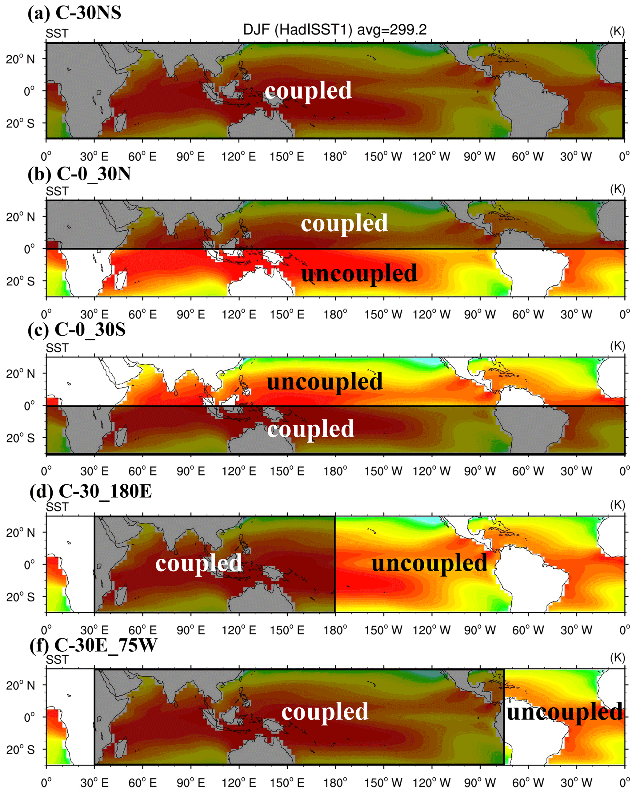
Figure 1 Schematics of coupled and uncoupled domains in the regional coupling experiment: (a) C–30NS, (b) C–0_30N, (c) C–0_30S, (d) C–30_180E, and (e) C–30E_75W. The background is the climatological mean SST in December–February (DJF).

3 Results and discussion

The realistic simulation of the MJO has always been a major bottleneck in the development of climate models. In this section, we demonstrate that the sensitivity of air–sea coupling experiments using a 1-D high-resolution ocean model significantly improves the MJO simulation by the CAM5.3. The period between November and April when the MJO is the most prominent was the targeted season in this study.

3.1 Improvement of MJO simulation through air–sea coupling

This subsection compares the MJO simulation of the control coupled experiment (C–30NS) with that of the uncoupled AGCM (A–CTL) forced by climatological monthly SST of HadISST1 to demonstrate the effect of air–sea coupling on the MJO simulation by coupling the SIT model to the CAM5.3 in the tropical belt (30^∘ N–30^∘ S).

3.1.1 Wavenumber–frequency spectra and eastward propagation characteristics

A wavenumber–frequency spectrum (W–FS) analysis was conducted to quantify propagation characteristics simulated in different experiments. The spectra of unfiltered U850 in ERA-I reanalysis, C–30NS, and A–CTL are shown in Fig. 2a–c, respectively. The C–30NS considering the coupling in 30^∘ N–30^∘ S realistically simulates eastward-propagating signals at zonal wavenumber 1 and 30–80 d periods (Fig. 2a and b) though with a slightly larger amplitude compared with ERA-I. By contrast, the uncoupled A–CTL does not yield realistic simulation; instead, it simulates both eastward-propagating (wavenumber 1) and westward-propagating (wavenumber 2) signals with an unrealistic spectral shift to timescales longer than 30–80 d.

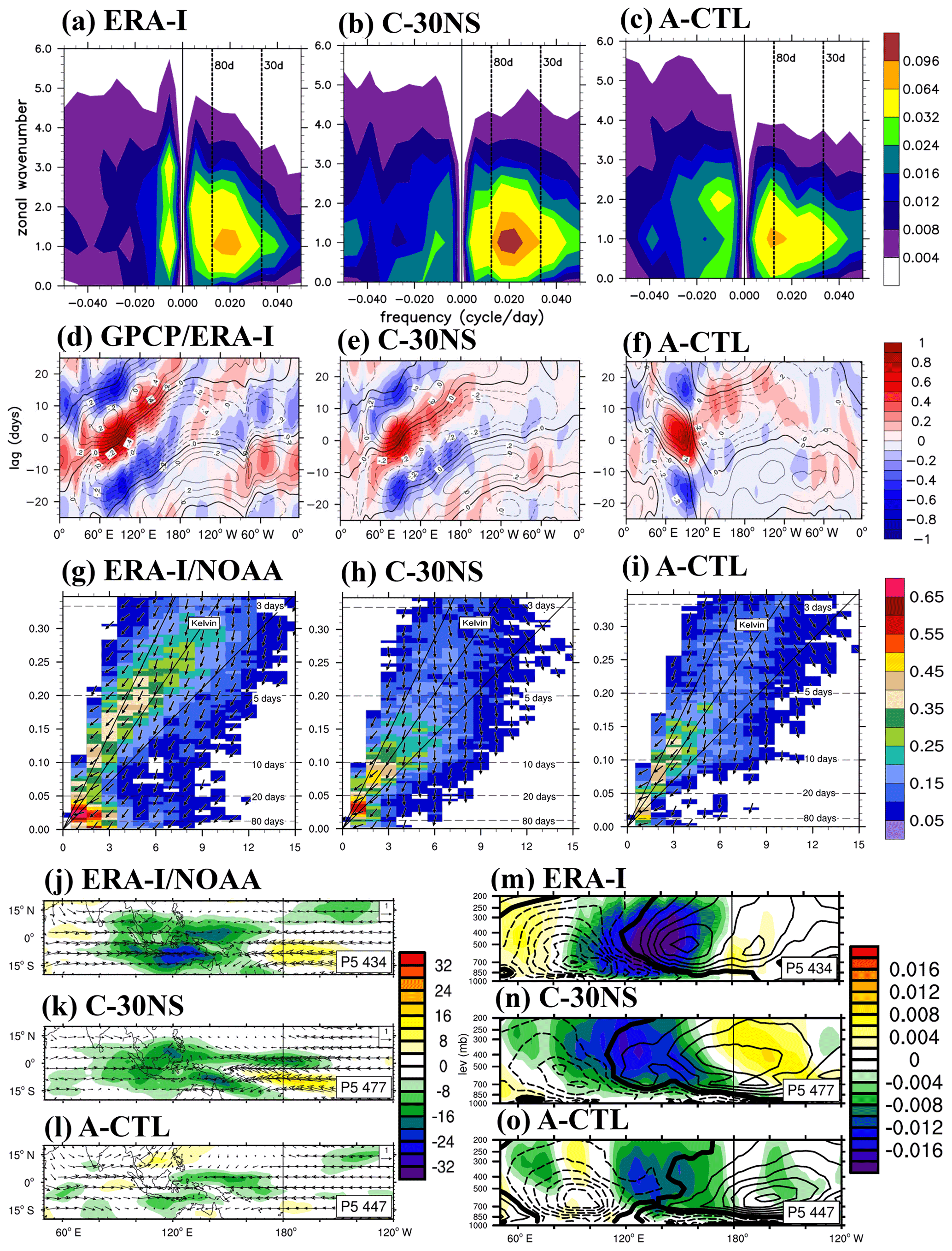
Figure 2 (a–c) Zonal wavenumber–frequency spectra for 850 hPa zonal wind averaged over 10^∘ S–10^∘ N in boreal winter after removing the climatological mean seasonal cycle. Vertical dashed lines represent periods at 80 and 30 d, respectively. (d–f) Hovmöller diagrams of the correlation between the precipitation averaged over 10^∘ S–5^∘ N, 75–100^∘ E and the intraseasonally filtered precipitation (color) and 850 hPa zonal wind (contour) averaged over 10^∘ N–10^∘ S. (g–i) Zonal wavenumber–frequency power spectra of anomalous OLR (colors) and phase lag with U850 (vectors) for the symmetric component of tropical waves, with the vertically upward vector representing a phase lag of 0^∘ with phase lag increasing clockwise. Three dispersion straight lines with increasing slopes represent the equatorial Kelvin waves (derived from the shallow water equations) corresponding to three equivalent depths, 12, 25, and 50 m, respectively. (j–l) Composites of 20–100 d filtered OLR (W m⁻²; shaded) and 850 hPa wind (m s⁻¹; vector) for MJO phase 5 when deep convection is the strongest over the MC and 850 hPa wind, with the reference vector (1 m s⁻¹) shown at the top right of each panel, and (m–o) 15^∘ N–15^∘ S averaged vertical pressure velocity anomaly (Pa s⁻¹; shaded) and moist static energy tendency anomaly (W m⁻², contour, interval 0.003); solid, dashed, and thick black lines represent positive, negative, and zero values, respectively. The number of days used to generate the composite is shown at the bottom right corner of each panel. Panels (a), (d), (g), (j), and (m) are from the ERA-Interim and NOAA post-processed data (ERA-I/NOAA); panels (b), (e), (h), (k), and (n) are from the control experiment C–30NS; and panels (c), (f), (i), (l), and (o) are from the A–CTL.

The major features of the simulated MJO propagation were examined. Figure 2d–f show the time evolution of precipitation and U850 anomalies in Hovmöller diagrams, which represent lagged correlation coefficients between the precipitation averaged over 10^∘ S–5^∘ N, 75–100^∘ E and the precipitation and U850 averaged over 10^∘ N–10^∘ S on intraseasonal timescales. Figure 2d indicates eastward propagation for both precipitation and U850 from the eastern IO to the dateline, with precipitation leading U850 by approximately a quarter of a cycle. The Hovmöller diagram derived from the C–30NS (Fig. 2e) exhibits the key characteristics of eastward propagation for both precipitation and U850 and the relative phases between the two, although the simulated correlation is slightly weaker than that derived from GPCP and ERA-I. By contrast, the uncoupled A–CTL simulates intraseasonal signals that propagate westward over the IO and weak and much slower eastward propagation crossing the MC and WP (Fig. 2f). The contrast between Fig. 2e and f demonstrates that coupling a 1-D TKE ocean model alone could lead to a significant improvement in an AGCM in simulating the major characteristics (e.g., amplitude, propagation direction and speed, and phase relationship between precipitation and circulation) of the MJO.

3.1.2 Coherence of the simulated MJO

Cross-spectral analysis was conducted to examine the coherence and phase lag between tropical circulation and convection, which were plotted over the tropical wave spectra. Figure 2g–i show the symmetric part (e.g., Wheeler and Kiladis, 1999) of OLR and U850 in ERA-I/NOAA data, C–30NS, and A–CTL, respectively. We present only the spectra between 0 and 0.35 d⁻¹ to highlight the MJO and equatorial Kelvin waves. The most prominent characteristics seen in ERA-I/NOAA data are the peak coherence at wavenumbers 1–3 and a phase lag of approximately 90^∘ in the 30–80 d band (Ren et al., 2019; Wheeler and Kiladis, 1999). The coupled experiment C–30NS simulates strong coherence in this low-frequency band (wavenumber 1) and exhibits a realistic phase lag relationship between U850 and OLR perturbations. However, the coherence at wavenumbers 2–3 for the 30–80 d period simulated by C–30NS is weaker than in ERA-I/NOAA data. This under-simulation was also noted in CCSM4 (Subramanian et al., 2011), the uncoupled and coupled CAM4 and CAM5 (Li et al., 2016), and NorESM1-M (Bentsen et al., 2013), which had a version of the CAM as an AGCM. In summary, C–30NS considering the coupling between 30^∘ N–30^∘ S produces coherent and energetic patterns in the eastward-propagating intraseasonal fluctuations of U850 and OLR in the tropical IO and WP that are generally consistent with the MJO characteristics. By contrast, the MJO characteristics in A–CTL are considerably weaker than those in C–30NS and in ERA-I/NOAA data.

3.1.3 Horizontal and vertical structures of the MJO across the MC

Figure 2j–o show the horizontal and vertical structures of the MJO when deep convection is the strongest over the MC (i.e., phase 5). Figure 2j–l present the 20–100 d filtered OLR (W m⁻²; shaded) and 850 hPa wind (m s⁻¹; vector). C–30NS realistically simulated the enhanced tropical convection over the eastern IO and the Kelvin-wave-like easterly anomalies over the tropical WP despite under-simulating the convection over the MC (Fig. 2j and k). By contrast, A–CTL failed to simulate the enhanced convection over the eastern IO and MC; instead, it simulated considerably weaker convection and easterly winds over the MC and WP, respectively, than that in ERA-I/NOAA data (Fig. 2j and l).

Figure 2m–o show the vertical–longitudinal profiles of 20–100 d filtered 15^∘ N–15^∘ S averaged vertical velocity (OMEGA; Pa s⁻¹; shaded) and moist static energy tendency ($\mathrm{d}\text{MSE}/\mathrm{d}t$) anomalies (W m⁻²; contour) at phase 5. The spatial distribution of negative OMEGA (ascending motion) anomalies generally agreed with OLR anomalies in C–30NS simulation and NOAA data over the Indo-Pacific region (Fig. 2m and n). The relatively spatial relationship between the ascending motion and $\mathrm{d}\text{MSE}/\mathrm{d}t$ seen in ERA-I is simulated well in the coupled experiment C–30NS. For example, positive $\mathrm{d}\text{MSE}/\mathrm{d}t$ anomalies on the eastern side of the anomalous ascent demonstrate that the energy recharge process occurs in advance of the MJO convection over the lower-tropospheric easterlies (Fig. 2m and n), whereas negative $\mathrm{d}\text{MSE}/\mathrm{d}t$ anomalies on the western side reveal that the discharge process occurs during and after convection over the lower-tropospheric westerlies. By contrast, this phase relationship, considered to be an essential feature leading to the eastward propagation of an MJO (Hannah and Maloney, 2014; Heath et al., 2021), is not properly simulated in the uncoupled experiment A–CTL (Fig. 2o), in which the simulated weak negative OMEGA is located between negative and positive $\mathrm{d}\text{MSE}/\mathrm{d}t$ anomalies over weak lower-tropospheric wind anomalies and associated with weak convection over the MC (Fig. 2l).

The temporal evolution of NOAA OLR and ERA-I U850 (Fig. 3a) indicates that convection originating in the western IO is enhanced during its eastward propagation to the MC where it reaches the peak amplitude and is then gradually weakened when continuing moving eastward to the dateline. In the coupled experiment C–30NS, this evolution of convectively coupled circulation is realistically simulated, although it is weaker than the strength seen in NOAA OLR (Fig. 3b). Moreover, the split of convection into two cells off the Equator in phase 6 is appropriately simulated in C–30NS (P6 in Fig. 3a and b). This split was caused by the topographic and land–sea contrast effects of the MC (Tseng et al., 2017). Associated with the split is the southward detour of the anomalous convection during the passage of the MJO through the MC (Kim et al., 2017; Tseng et al., 2017; Wu and Hsu, 2009). After the passage of the MJO through the MC, the anomalous convection stays south of the Equator and continues moving eastward to the dateline. In the uncoupled A–CTL, the systematic eastward propagation of convectively coupled MJO circulation from the IO into the MC is not simulated. Instead, the convection over the MC develops in situ at a later stage than that observed (e.g., P6 in Fig. 3c) and dissipated rapidly. The A–CTL simulates a pair of off-Equator convection anomalies in the eastern IO during phase 2 (P2 in Fig. 3c) that moves westward toward the central IO and is amplified at later stages (e.g., P4 in Fig. 3c). This unrealistic evolution explains the westward propagation tendency observed in the Hovmöller diagram (Fig. 2f).

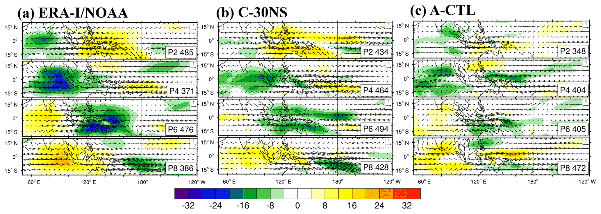
Figure 3 Evolution of the filtered OLR anomaly (W m⁻²; shaded) and 850 hPa wind (m s⁻¹; vector) at phase 2, 4, 6, and 8: (a) the ERA-I/NOAA data, (b) the control coupled experiment C–30NS, and (c) the uncoupled experiment A–CTL. The unit of the reference vector shown at the top right corner of each panel is meters per second (m s⁻¹), and the number of days used for the composite is shown in the bottom right corner of each panel.

3.1.4 Characteristics of air–sea interaction

Figure 4a–c show the longitude–phase diagram in which the 20–100 d filtered precipitation (shaded) and SST (contour) anomalies were averaged over 10^∘ S–10^∘ N to determine the relationship between precipitation and SST fluctuations and to establish a link between air–sea coupling and convection. The propagation of the enhanced convection with positive SST anomalies to the east could be clearly seen in GPCP/OISST and the coupled experiment C–30NS (Fig. 4a and b). The highest SST anomaly (SSTA) leads the maximum precipitation anomaly by approximately 2–3 phases, and the SSTA begins to decrease following the onset of enhanced precipitation. The ERA-I and OISST data reveal the following relationship between net surface flux and SST: the decreased (increased) LHF and SHF and increased (decreased) downward radiation flux leads (lags behind) the positive (negative) SSTA east (west) of anomalous deep convection. This well-known lead–lag relationship reflecting the active air–sea interaction in an MJO is realistically simulated in the coupled experiment C–30NS (not shown).

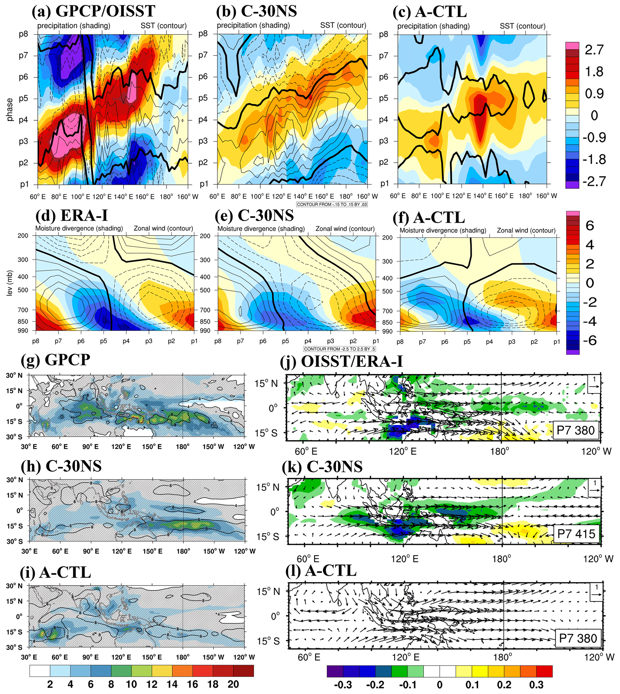
Figure 4 (a–c) Phase–longitude Hovmöller diagrams of 20–100 d filtered precipitation (mm d⁻¹; shaded) and SST anomaly (K, contour) averaged over 10^∘ N–10^∘ S from phase 1 to 8. Contour interval is 0.03; solid, dashed, and thick black lines represent positive, negative, and zero values, respectively. (d–f) Phase–vertical Hovmöller diagrams of 20–100 d moisture divergence (shading; 10⁻⁶ $\mathrm{g}{\mathrm{kg}}^{-\mathrm{1}}{\mathrm{s}}^{-\mathrm{1}}$) and zonal wind (contoured; m s⁻¹) averaged over 10^∘ N–10^∘ S, 120–150^∘ E; solid, dashed, and thick black curves are positive, negative, and zero values, respectively. (g–i) Variation of 30–60 d filtered precipitation in the eastern IO and the WP in observation (color shading) and the ratio between intraseasonal and total variance (contoured) and (j–l) composites 20–100 d filtered SST (K; shaded) and 850 hPa winds (m s⁻¹; vector) at phase 7 when deep convection was the strongest over the dateline. Reference vector shown in the top right corner of each panel. Panels (a), (d), (g), and (j) are from the ERA-I/NOAA data; panels (b), (e), (h), and (k) are from the control coupled experiment C–30NS; and panels (c), (f), (i), and (l) are from the uncoupled experiment A–CTL.

The contrast between C–30NS and A–CTL confirms the key role of the air–sea interaction in contributing to the eastward propagation and demonstrates that the eastward propagation simulation can be markedly improved by incorporating the air–sea interaction process in the model, even when using a simple 1-D ocean model such as SIT.

3.1.5 Vertically tilting structure

The warm SST was the key forcing that contributed to the boundary layer convergence before the onset of deep convection (Li et al., 2020; Tseng et al., 2014). Hence, the warmer upper ocean enhances the low-level atmospheric convergence and then leads to enhanced low-level moisture and preconditioned deep convection and eastward propagation. This moistening process associated with warm ocean surface temperature is simulated well in the coupled experiment C–30NS but is not shown here. Instead, we present the coupling of moisture divergence (MD) and atmospheric circulation.

MD and zonal wind anomalies from the surface to the upper troposphere averaged over the 10^∘ S–10^∘ N and 120–150^∘ E region are shown in Fig. 4d–f to depict the relationship between the vertically tilting structure of MD and zonal wind anomalies. Note that the active convection occurred around phase 5. The coupled experiment C–30NS (Fig. 4e) realistically simulates the deepening of coupled MD and zonal wind anomalies with time (Fig. 4d). An evolution from the right to left seen in each panel of Fig. 4d–f is equivalent to the eastward movement of vertically tilting circulation from the eastern IO into the MC because of the eastward-propagating nature of the MJO. Figure 4d and e show that in both ERA-I reanalysis and the coupled experiment C–30NS, the near-surface convergence (negative MD) occurring in the easterly anomalies leads the convection and continued deepening up to 500 hPa from phase 2 to phase 6 when the easterly anomalies switch to westerly anomalies. By contrast, this evolution of coupled MD–zonal wind anomalies are not appropriately simulated in the uncoupled experiment (Fig. 4f). For example, a slow deepening with time is observed in the MD anomaly but not in the zonal wind anomaly that exhibits a vertically decayed structure, suggesting that MD and wind anomalies are not well coupled, as noted in the ERA-I/NOAA data and the control coupled experiment.

In the ERA-I reanalysis data, the negative near-surface MD anomalies appear first under the easterly anomaly and continue deepening between the easterly and westerly anomalies. This development in the phase relationship between MD and zonal wind anomalies in both ERA-I reanalysis data and the coupled simulation is consistent with the well-known structure embedded in the MJO, namely the near-surface convergence in the easterly phase (i.e., a boundary-layer moistening process; Kiranmayi and Maloney, 2011; Li et al., 2020; Tseng et al., 2014), followed by the deep convection when transitioning to the westerly phase. This close phase relationship that is key to the eastward propagation is appropriately simulated in the coupled experiment but not in the uncoupled experiment.

3.1.6 Intraseasonal variance of precipitation

Figure 4g–i present the spatial distribution of intraseasonal variance of precipitation. In the GPCP data, the maximum variance is noted over the tropical eastern IO, MC, and tropical WP. The maximum variance south of the island in the MC and the Equator in the tropical WP reflects the southward shift of the MJO deep convection when passing through the MC, partly due to the blocking effect of mountainous islands and the higher moisture content over high SST south of the Equator in the region during boreal winter (Kim et al., 2017; Ling et al., 2019; Sobel et al., 2008; Tseng et al., 2017; Wu and Hsu, 2009). Although the control coupled experiment fails to simulate the variance maximum in the tropical eastern IO, it appropriately simulates the maximum variance over the tropical WP, reflecting its ability to simulate the eastward propagation of the MJO through the MC. By contrast, the uncoupled A–CTL experiment simulates considerably weaker intraseasonal variance in both the tropical eastern IO and the tropical WP. Figure 4j–l are the 20–100 d filtered SST (K; shaded) and 850 hPa wind (m s⁻¹; vector) during MJO phase 7 when deep convection is the strongest over the dateline. The coupled experiment C–30NS realistically simulates the negative SST anomaly over the MC and WP when enhanced tropical convection passed through the MC to the dateline, indicating the capability of the SIT model to reproduce the SST anomaly by exchanging LHF and SHF between the atmosphere and ocean. In A-CTL, no SST anomaly is evident because the model was forced by prescribed climatological SST. The contrast seen in Fig. 4j–l demonstrates the essential role of atmosphere–ocean coupling in shaping the MJO. A delayed air–sea interaction mechanism was noted, where a preceding active-phase MJO may trigger an inactive-phase MJO through the delayed effect of the induced SST anomaly. In addition, the westerly winds at 850 hPa moving southward between MC and WP are captured by the control experiment C–30NS and are similar to the ERA-I reanalysis winds (Fig. 4j and k). By contrast, A–CTL forced by climatological monthly SST (<0.05 K phase⁻¹ anomaly) fails to simulate the southward westerly wind of the region extending from the MC to the dateline (Fig. 4l).

3.2 Effect of upper-ocean vertical resolution

In the control coupled experiment C–30NS, the vertical resolution in the upper 10.5 m was 1 m. Tseng et al. (2014) suggested that fine vertical resolution is crucial for appropriately simulating the eastward propagation. To investigate the effect of vertical resolution, two experiments with a thicker first layer were conducted by moving the center of the layer to 11.5 m (C–LR12m) and 33.9 m (C–LR34m), respectively, as opposed to the control experiment in which 10 layers were implemented in the first 10.5 m (see Appendix Fig. A1 for vertical discretization). The dramatic changes in vertical profile of ocean temperature between the fine- and coarse-resolution simulation are demonstrated in Fig. 5, which presents the 20–100 d filtered oceanic temperature anomalies (K; shaded) between 0 and 60 m depth for MJO phase 1, 3, 5, and 7. The amplitude of ocean temperature is the largest in C–30NS and much weaker in C–LR12m and C–LR34m. In addition, there is a clear vertical stratification of ocean temperature in C–30NS, whereas C–LR12m and C–LR34m are well mixed because there is no vertical gridding. This demonstrates the necessity of fine vertical gridding for resolving the quick fluctuation of ocean temperature when interacting with the atmosphere.

Figure 5 Composites of 20–100 d filtered oceanic temperature (K; shaded) between 0 and 60 m depth for MJO phase 1, 3, 5, and 7 (shown in the lower right corner of each panel) in C–30NS, C–LR12m, and C–LR34m.

The W–FS spectral peaks of U850 in C–LR12m are concentrated in eastward-propagating wavenumber 1 at three timescales (e.g., longer than 80 d, 30–80 d, and approximately 30 d; Fig. 6a). In C–LR34m, both eastward and westward signals are simulated with the dominant W–FS timescale longer than 80 d (Fig. 6b). The appearance of both eastward and westward signals at a lower frequency implied a stronger stationary tendency or weaker eastward-propagating tendency. This result is consistent with that reported by Tseng et al. (2014) that the scientific reproducibility of coarser resolution causes a longer intraseasonal periodicity and slower eastward propagation of the MJO.

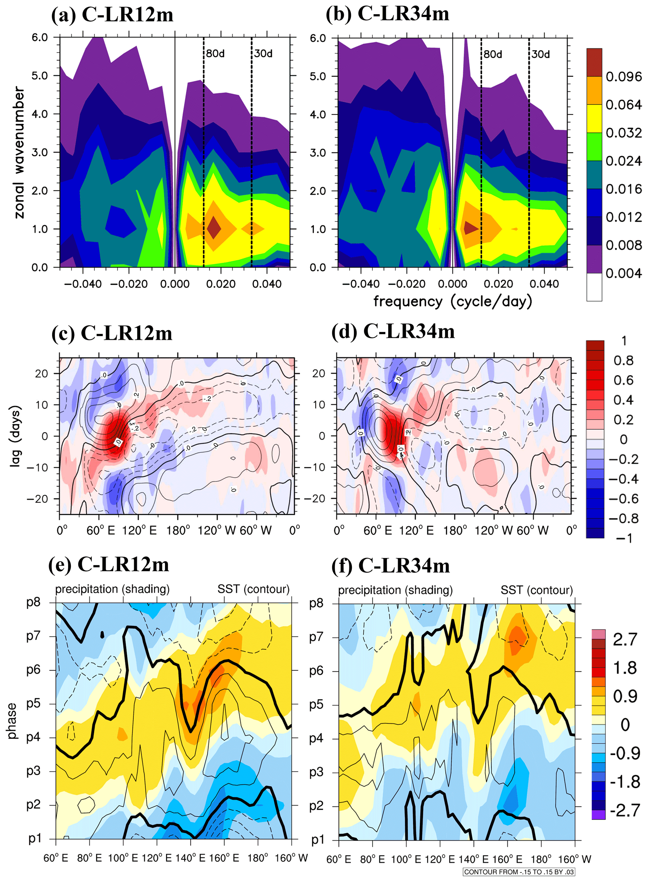
Figure 6 (a, b) Same as in Fig. 2a but for the C–LR12m and C–LR34m. (c, d) Same as in Fig. 2d but for the C–LR12m and C–LR34m. (e, f) Same as in Fig. 4a but for the C–LR12m and C–LR34m.

The effect of vertical resolution on the MJO simulation can be seen in the Hovmöller diagram. The eastward propagation simulated in C–LR12m (Fig. 6c) markedly weakened after crossing the MC compared with that simulated in the control experiment C–30NS (Fig. 2e). In C–LR34m, the quasi-stationary fluctuation and westward propagation are simulated over the IO (Fig. 6d), appearing similar to those in A–CTL (Fig. 2f). The lead–lag relationship between precipitation (zonal wind) and SST is poorly simulated in C–LR12m (Fig. 6e) and even more poorly simulated in C–LR34m (Fig. 6f). This result confirms the finding reported by Tseng et al. (2014) that a higher vertical resolution in the upper few meters below the surface allows for a faster air–sea interaction, thus resulting in a more realistic simulation of the MJO.

3.3 Effect of the lowest boundary of the SIT model

The ocean is a vital energy source for the MJO. Although vertical resolution is crucial for the efficiency of air–sea interaction, the thickness of the upper ocean that interacts with the atmosphere represents the ocean heat content to substantiate the MJO. A key question is how the total ocean heat content, which depends on the total depth of the ocean, can affect the MJO. Considering two models with the same vertical resolution, the model with thinner ocean (e.g., 10 m) would interact as efficiently as another model with thicker ocean (e.g., 60 m) but with much less heat to release to or to absorb from the atmosphere. The former would have less impact on the atmosphere than the latter. Using the same vertical resolution, three experiments with various ocean bottoms at 10, 30, and 60 m were conducted (see Appendix Fig. A2 and Table 1).

The spectra and the Hovmöller diagrams shown in Fig. 7a–c and d–f, respectively, demonstrate that the thicker ocean model simulates a stronger MJO with a frequency closer to that in the coupled experiment C–30NS and ERA-I/NOAA data and more realistic eastward propagation. In addition, the lead–lag relationship between precipitation (wind) and SST is more realistically simulated with increasing thickness of the ocean model (Fig. 7g–i).

Figure 7 Same as in Fig. 6 but for the C–HR1mB10m, C–HR1mB30m, and C–HR1mB60m.

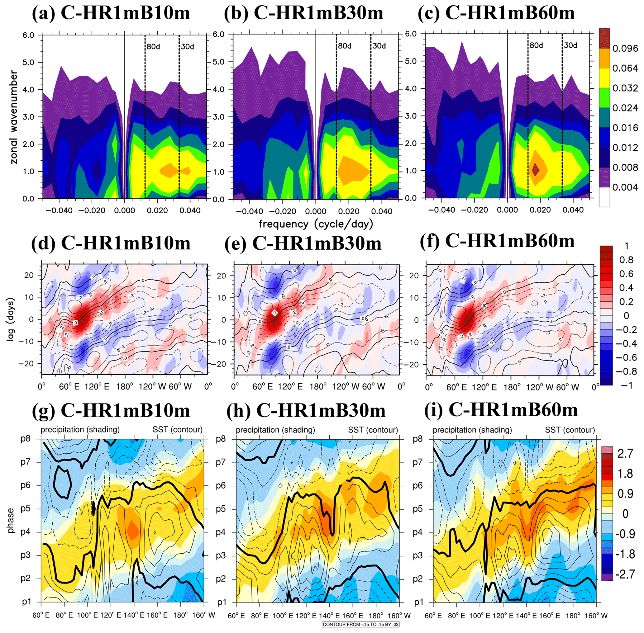
This result suggests that the thickness of the vertically gridded ocean that interacts with the atmosphere strongly affects the frequency of the simulated MJO. A thinner (thicker) vertically gridded ocean is more quickly (slowly) recharged and discharged through SHF and LHF exchange between the atmosphere and ocean and therefore likely fluctuates at a faster (slower) tempo. The simulated periodicity is therefore affected by the thickness (or ocean heat content) of upper ocean that interacts rigorously with the atmosphere. Although the result suggests 60 m is an appropriate thickness to realistically simulate the periodicity of the MJO, we did not intend to suggest the exact thickness required for a proper simulation because it might depend on the model. The upper ocean should be adequately thick to contain a certain amount of heat to generate appropriate periodicity. However, the reason for the intraseasonal timescale (i.e., 20–100 d) should be determined in future studies. This finding does not suggest a constant periodicity because periodicity might be affected by the time-varying structure of the atmosphere and ocean in the real world.

3.4 Effects of coupling domains

The MJO is a planetary-scale phenomenon. Given its large-scale circulation, the air–sea interaction affecting the MJO likely occurs in a much larger area than the region near the major convection anomalies. In this section, we discuss the effect of coupling domain on model ability to simulate the eastward propagation speed and periodicity of the MJO. Four experiments considering the coupling in various domains (C–0_30N, C–0_30S, C–30_180E, and C–30E_75W, Fig. 1) were conducted for this purpose. The results are shown in Fig. 8. The C–0_30N that considered the coupling in the tropics between the Equator and 30^∘ N simulates the least realistic MJO propagation in terms of W–FS (Fig. 8a), zonal wind–precipitation coupling (Fig. 8e), and SST–precipitation (Fig. 8i) among the four regional coupling experiments. By contrast, coupling only the tropics between the Equator and 30^∘ S simulates a more realistic MJO in all three aspects (i.e., spectrum in Fig. 8b and temporal evolution of precipitation–wind and precipitation–SST coupling in Fig. 8f and j). Fig. 9a indicates that the negative OLR anomalies at phase 5 simulated in C–0_30N stay mainly north of the Equator and do not shift southward in the MC as revealed in ERA-I reanalysis and NOAA OLR and in the control experiment C–30NS, and the convection over the IO is unrealistically weak. By contrast, the southward detouring in the MC is realistically simulated in C–0_30S that coupled only the tropical ocean between the Equator and 30^∘ S. This result indicates that air–sea coupling occurring south of the Equator is the key to producing appropriate eastward propagation and detouring of the MJO through the MC. Without this coupling, the C–0_30N experiment fails to realistically simulate the eastward propagation of the MJO (Fig. 8e). This contrast can be attributed to the warmer ocean surface and higher moisture content found south of the Equator in boreal winter, which comprise a more favorable environmental condition for air–sea coupling and convection–circulation coupling and the occurrence of the MJO.

Figure 8 Same as in Fig. 6 but for the C–0_30N, C–0_30S, C–30_180E, and C–30E_75W.

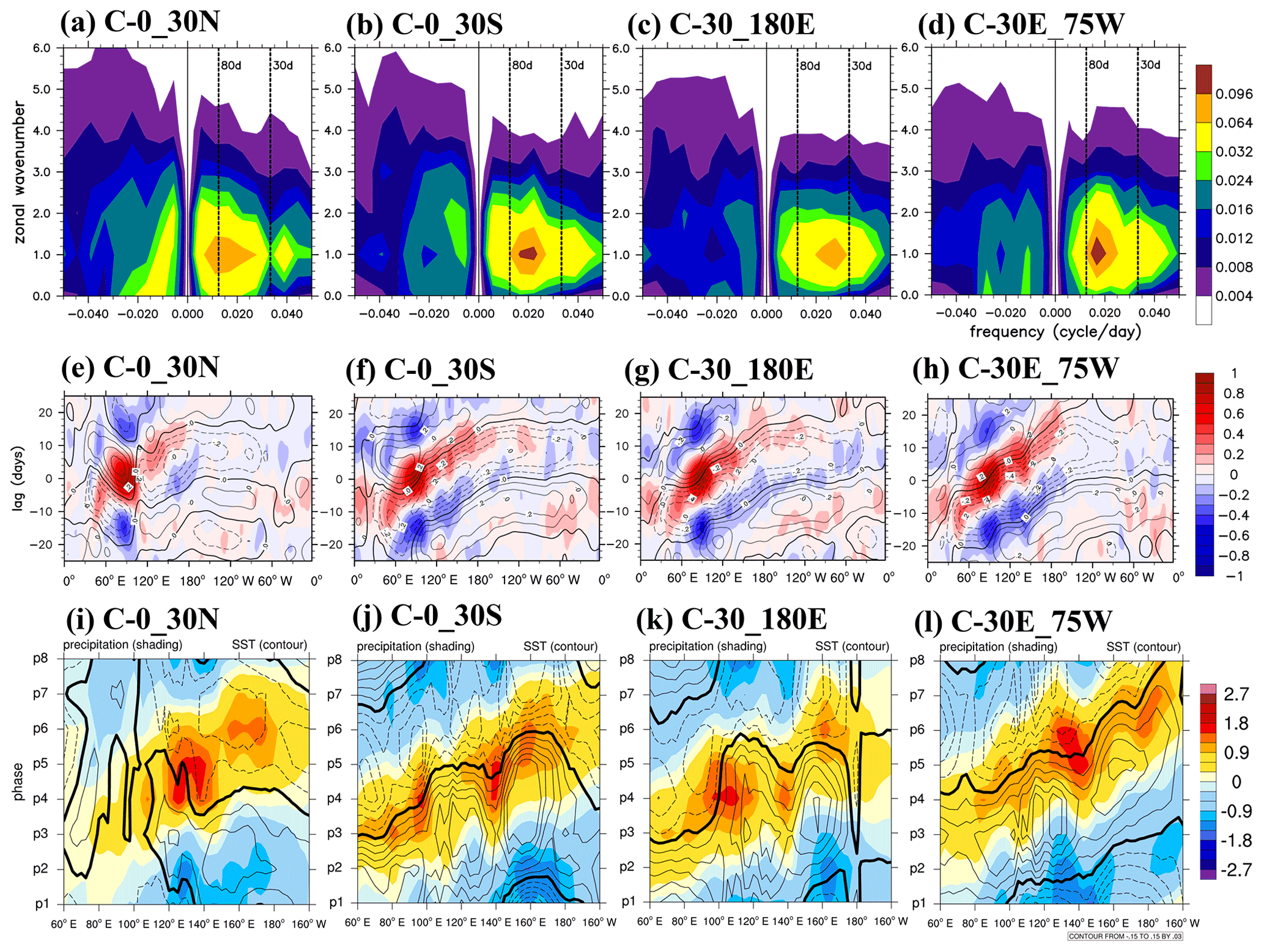
MJO simulations can be affected by air–sea coupling in the longitudinal domain. Tseng et al. (2014) examined this effect by allowing for coupling in different regions (e.g., the IO, WP, and IO + WP) and found that the IO + WP coupling experiment yielded the most satisfactory MJO simulation in terms of the zonal W–FS and eastward propagation characteristics. In this study, we conducted sensitivity experiments in which we allowed for coupling in the tropics in two longitudinal domains, namely 30–180^∘ E (C–30_180E) and 30^∘ E–75^∘ W (C–30E_75W). The 30–180^∘ E region covered the IO and WP, and the 30^∘ E–75^∘ W region covered the IO and the entire tropical Pacific. As shown in Fig. 8, the C–30E_75W experiment simulates a more realistic MJO than the C–30_180E experiment, with stronger eastward propagation and larger amplitudes in the spectrum (Fig. 8c and d) and Hovmöller diagrams of precipitation/wind (Fig. 8g and h) and precipitation/SST (Fig. 8k and l). The simulated MJO in C–30E_75W propagated farther east than that in C–30_180E, particularly evident in Fig. 8k and l. The spatial distributions of circulation and OLR shown in Fig. 9c and d indicate the presence of a stronger convection–circulation coupling system over the MC and WP in C–30E_75W. These results suggest that coupling over the entire tropical IO and Pacific could enhance the strength and eastward propagation of the MJO and encourage farther propagation to the central Pacific.

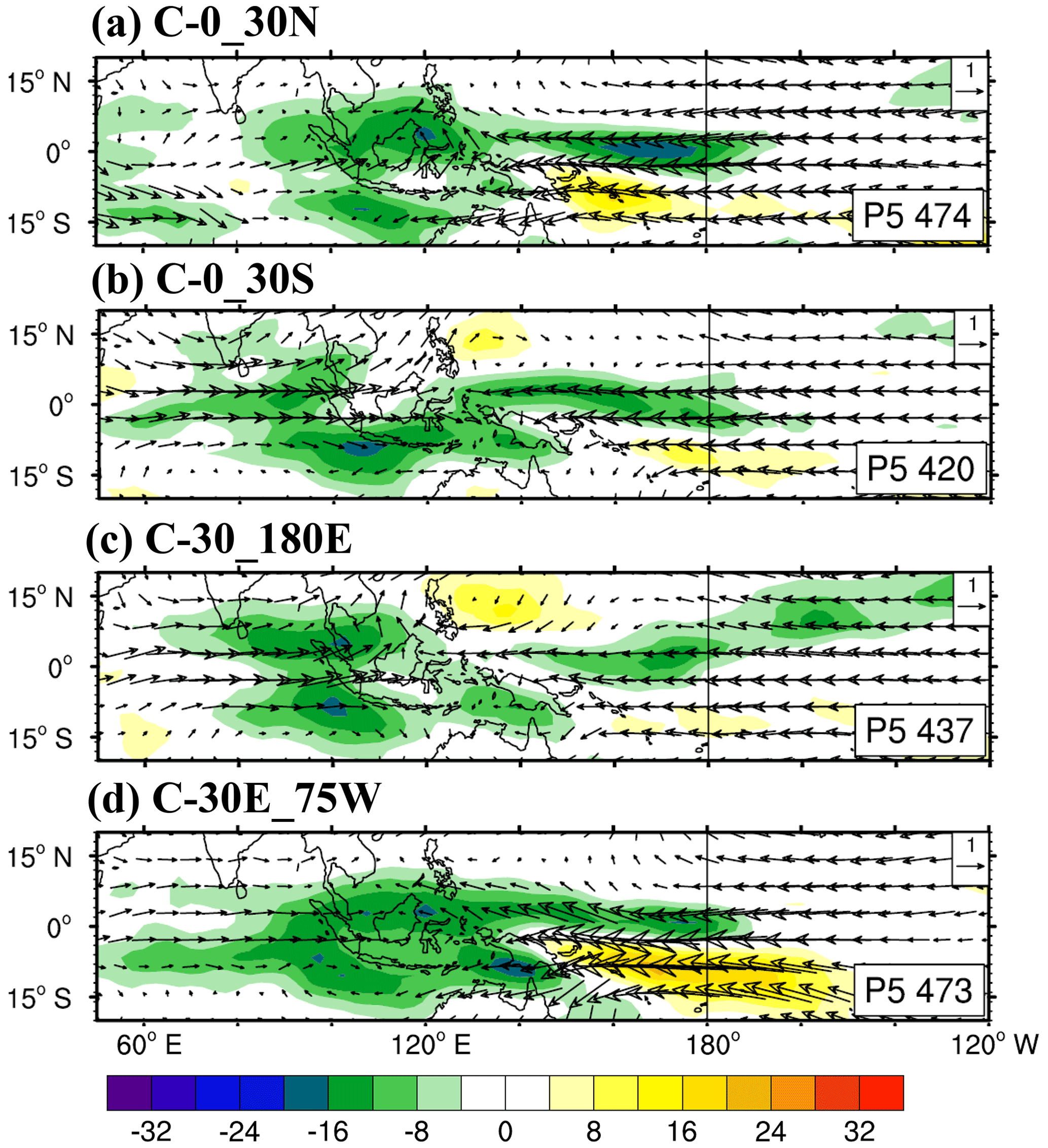
Figure 9 Same as in Fig. 3 but for phase 5 in the C–0_30N, C–0_30S, C–30_180E, and C–30E_75W.

3.5 Diurnal versus no diurnal cycle in air–sea coupling

Previous studies showed that the diurnal cycle in the MC can weaken the MJO and its eastward propagation (Hagos et al., 2016; Oh et al., 2013). We conducted an experiment to determine whether computing surface heat fluxes using daily mean values, instead of instantaneous values, of atmospheric variables and SST with the same coupling frequency would affect the MJO simulation. The coupling in the model was conducted through the SHF and LHF exchange between the atmosphere and ocean, which were calculated based on simulated winds, moisture, and temperature. As mentioned in Sect. 2.3, air–sea fluxes were calculated twice for every time step (coupling 48 times per day) in the control coupled experiment (C–30NS) based on the instantaneous values of atmospheric and oceanic variables. In the experiment in which the diurnal cycle was removed (C–30NS–nD), air–sea fluxes were calculated as in C–30NS but were based on daily means of both atmospheric variables and SST. Doing this removed certain diurnal effects of air-sea coupling. The results shown in Fig. 10 reveal the enhancement of the eastward-propagating signals in the MJO (e.g., a larger amplitude in spectrum; Fig. 10a) and further eastward propagation (Fig. 10b) as well as stronger coupling between precipitation and SST (Fig. 10c) in C–30NS–nD. The overall results are consistent with the previous finding that the diurnal cycle tends to reduce the amplitude of the MJO, indicating that the weakening effect occurs through air–sea coupling in addition to those processes in the atmosphere. Previous studies have hypothesized that rapid interaction processes in the diurnal timescale tend to extract energy from the MJO, thus reducing the strength and propagation tendency of the MJO. However, a comparison between the spectra of C–30NS and C–30NS–nD indicates that the experiment in which the diurnal cycle is removed appeared to over-simulate the MJO with unrealistic strength, suggesting that the effect of the diurnal cycle should be considered in the model to simulate a more realistic MJO. However, whether this is a common result in different models remains to be examined.

Figure 10 Similar as in Fig. 6 but for the C–30NS–nD.

4 Discussion and conclusions

Air–sea coupling is a key mechanism for the successful simulation of the MJO (Chang et al., 2019; DeMott et al., 2015; Jiang et al., 2015, 2020; Kim et al., 2010; Li et al., 2016, 2020; Newman et al., 2009; Tseng et al., 2014). This study, following the study of Tseng et al. (2014), demonstrated that coupling a high-resolution 1-D TKE ocean model (namely the SIT model) to the CAM5, namely the CAM5–SIT, significantly improved the MJO simulation over the standalone CAM5. By coupling SIT model to an AGCM different from Tseng et al. (2014), this study confirms the scientific reproducibility for the improvement of MJO simulation in modeling science. The CAM5–SIT realistically simulates the MJO characteristics in many aspects (e.g., intraseasonal periodicity, eastward propagation, coherence in the low-frequency band, detouring propagation across the MC, tilting vertical structure, and intraseasonal variance in the WP). Systematic sensitivity experiments were conducted to investigate the effects of the vertical resolution and the thickness of the 1-D ocean model, coupling domains, and the absence of the diurnal cycle. The results of all the sensitivity experiments are summarized in Fig. 11a and b, which show four common metrics for MJO evaluation. The four metrics are the propagation speed of the MJO (estimated from the U850 Hovmöller diagram as Fig. 2d–f) versus the power ratio of eastward- and westward-propagating 30–80 d signals (E$/$W ratio, derived from the zonal W–FS) in Fig. 11a and the eastward propagation speed of the 30–80 d filtered precipitation anomaly (estimated from the precipitation Hovmöller diagram) versus the variance explained by RMM1 and RMM2 (i.e., the sum of the variance explained by the first two empirical orthogonal functions (EOF1 and EOF2) based on Wheeler and Hendon, 2004) in Fig. 11b. Based on the maximum precipitation anomaly and zero values of U850 (indicating deep convection region), propagation speeds of precipitation and U850 were calculated from Hovmöller diagrams between 60^∘ E and 150^∘ W. Overall, the control experiment C–30NS simulates the most realistic MJO among all sensitivity experiments.

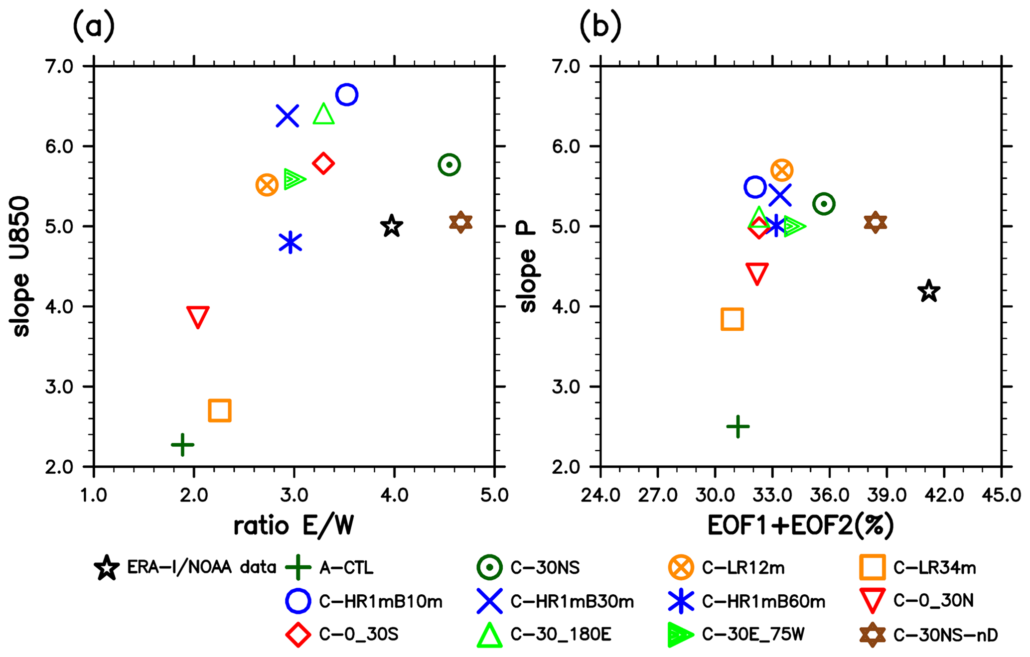
Figure 11 Scatter plots of various MJO indices in the ERA-I/NOAA data and 12 experiments: (a) power ratio of eastward-propagating to westward-propagating (E$/$W) waves of wavenumber 1–3 of 850 hPa zonal winds (x axis) with a 30–80 d period and eastward propagation speed of U850 anomaly (y axis) from the Hovmöller diagram. (b) RMM1 and RMM2 variance and eastward propagation speed of the filtered precipitation anomaly derived from the Hovmöller diagram.

As for vertical resolution, we determined that the MJO simulation efficiency decreased when the vertical resolution of the SIT model is decreased from 1 m to 11.5 or 33.9 m, as simulated in the C–LR12m and C–LR34m experiments, respectively. This finding, consistent with that reported by Tseng et al. (2014), suggests that a finer vertical resolution more effectively resolves temperature variations in the ocean warm layer and enhances atmospheric–ocean coupling, thus enabling the upper ocean to more efficiently respond to atmospheric forcing by providing sensible and latent heat fluxes; this results in superior synchronization between the lower atmosphere and the upper ocean.

We observed that the shallower ocean model bottom could speed up the eastward propagation of the MJO by producing more perturbations of shorter periodicity (Fig. 7) and results in a weaker MJO. The shallower ocean layer with vertical grids likely responds more quickly to atmospheric forcing but provides fewer sensible and latent heat fluxes to the atmosphere. Thus, the MJO propagates too fast with a weaker amplitude.

In the coupling domain sensitivity experiments, we investigated the essential coupling domain required to simulate the realistic MJO and the effect of the domain on the MJO simulation. Coupling only the northern tropics fails to simulate the eastward propagation, whereas coupling only the southern tropics yields a more realistic MJO simulation, although this simulation is inferior to coupling the entire tropics. This contrast reveals the importance of the southern tropical ocean, especially in the MC where high SST and moisture content are noted. Coupling in the southern tropics is therefore essential for providing the energy required to maintain the MJO and its eastward propagation. By contrast, the northern tropics are relatively dry and cool. Coupling in this region is therefore less effective in improving MJO simulation.

In the longitudinal domain sensitivity experiments, we found that the MJO amplitude and the eastward extend of its eastward propagation are enhanced by extending the eastern boundary of the coupling domain from the tropical eastern IO to the tropical WP and further to the tropical eastern Pacific (Fig. 1). Further extension of the domain to cover the tropical Atlantic does not exhibit further enhancement (not shown). This result indicates that coupling in the tropical central and eastern Pacific, although not the major MJO signal regions (i.e., from the tropical IO to the tropical WP), still played a marked role in sustaining the MJO. We propose the following to explain this effect. Because of the planetary scale of the MJO, the near-surface easterly circulation to the east of the convection core often extended to the tropical central and eastern Pacific, where the climatological easterly prevailed. The coupling beyond the WP increased low-level moisture transport and convergence to the east of the convection and established an environment suitable for the further eastward propagation of the MJO. This effect was likely terminated by the landmass of Central America when the tropical Atlantic was further included. Thus, a further eastward extension of the coupling domain exerted little effect on further enhancing the MJO. A diagnostic study on the effect of the longitudinal coupling domain is being conducted, and the results will be reported in a follow-up paper.

The diurnal versus nondiurnal cycle experiment indicates that nondiurnal coupling tended to enhance eastward-propagating signals but slow down the eastward propagation (Fig. 11a and b). This result is consistent with the finding of previous studies that the diurnal cycle in the atmosphere extracts energy from the MJO, thus weakening it.

In this study, we demonstrated how air–sea coupling can improve the MJO simulation in a GCM. The findings are as follows.

1. Better resolving the fine structure of the upper-ocean temperature and therefore the air–sea interaction leads to more realistic intraseasonal variability in both tropical SST and atmospheric circulation.

2. An adequate thickness of vertically gridded upper ocean is required to simulate a delayed response of the upper ocean to atmospheric forcing and lower-frequency fluctuation.

3. Coupling the tropical eastern Pacific, in addition to the tropical IO and the tropical WP, can enhance the MJO and facilitate the further eastward propagation of the MJO to the dateline.

4. Coupling the southern tropical ocean, instead of the northern tropical ocean, is essential for simulating a realistic MJO.

5. Stronger MJO variability can be obtained without considering the diurnal cycle in coupling.

Our study confirmed the effectiveness of air–sea coupling for improving MJO simulation in a climate model and demonstrated how and where to couple. The findings enhance our understanding of the physical processes that shape the characteristics of the MJO.

Appendix A: 1-D high-resolution TKE ocean model

The 1-D high-resolution turbulence kinetic energy ocean model SIT was used to simulate the diurnal fluctuation of SST and surface energy fluxes. The model was verified well against surface and subsurface observations in the South China Sea (Lan et al., 2010) and the tropical WP (Tu and Tsuang, 2005). Variations in sea water temperature (T), current (u), and salinity (S) were determined (Gaspar et al., 1990) using the following equations.

$$\begin{array}{}\text{(A1)}& {\displaystyle }& {\displaystyle \frac{\partial T}{\partial t}}=(k_{\mathrm{h}}+v_{\mathrm{h}}){\displaystyle \frac{{\partial }^{\mathrm{2}}T}{\partial z^{\mathrm{2}}}}+{\displaystyle \frac{R_{\text{sn}}}{{\mathit{\rho }}_{\text{w0}}{c}_{\mathrm{w}}}}{\displaystyle \frac{\partial F}{\partial z}}\text{(A2)}& {\displaystyle }& {\displaystyle \frac{\partial \mathit{u}}{\partial t}}=-f\mathit{k}\times \mathit{u}+(k_{\mathrm{m}}+v_{\mathrm{m}}){\displaystyle \frac{{\partial }^{\mathrm{2}}\mathit{u}}{\partial z^{\mathrm{2}}}}\text{(A3)}& {\displaystyle }& {\displaystyle \frac{\partial S}{\partial t}}=(k_{\mathrm{h}}+v_{\mathrm{h}}){\displaystyle \frac{{\partial }^{\mathrm{2}}S}{\partial z^{\mathrm{2}}}},\end{array}$$

where R_sn is the net solar radiation at the surface (W m⁻²), F(z) is the fraction (dimensionless) of R_sn that penetrates to the depth z, and k_h and k_m are eddy diffusion coefficients for heat and momentum (m² s⁻¹), respectively. The value of k_h within the cool skin layer and that of k_m within the viscous layer were set to zero. Molecular transport is the only mechanism for the vertical diffusion of heat and momentum in the cool skin and viscous layer, respectively (Hasse, 1971; Grassl, 1976; Wu, 1985). The parameters ν_m and ν_h are the molecular diffusion coefficients for momentum and temperature, respectively, ρ_w0 is the density (kg m⁻³) of water, and c_w is the specific heat capacity of water at constant pressure ($\mathrm{J}{\mathrm{kg}}^{-\mathrm{1}}{\mathrm{K}}^{-\mathrm{1}}$). S is salinity (‰), u is the current velocity (m s⁻¹), f is the Coriolis parameter (dimensionless), and k is the vertical unit vector (m s⁻¹).

Using the numerical solution of the surface layer (T₀), we disregard the time term of the 2 m air temperature (T_2m), which can be considered the upper boundary of an ocean, as well as the numerical solution of the surface longwave radiation T₀ term and aerodynamic resistance (r_a).

$$\begin{array}{}\text{(A4)}& \begin{array}{rl}{\displaystyle \frac{\partial T_{\mathrm{0}}}{\partial t}}=& {\displaystyle \frac{G_{\mathrm{0}}}{{\mathit{\rho }}_{\mathrm{w}}\cdot c_{\mathrm{w}}\cdot h_{\mathrm{e}}}}+{\displaystyle \frac{R_{\text{sn}}\left[F\right(z_{\mathrm{0}})-F(z_{\mathrm{0}}-d\left)\right]}{{\mathit{\rho }}_{\mathrm{w}}\cdot c_{\mathrm{w}}\cdot h_{\mathrm{e}}}}\\ & -{\displaystyle \frac{G_{\mathrm{0},\mathrm{1}}}{{\mathit{\rho }}_{\mathrm{w}}\cdot c_{\mathrm{w}}\cdot h_{\mathrm{e}}}}\\ =& {\displaystyle \frac{R_{\text{ld}}-R_{\text{lu}}-H-LE}{{\mathit{\rho }}_{\mathrm{w}}\cdot c_{\mathrm{w}}\cdot h_{\mathrm{e}}}}\\ & +{\displaystyle \frac{R_{\text{sn}}\left[F\right(z_{\mathrm{0}})-F(z_{\mathrm{0}}-d\left)\right]}{{\mathit{\rho }}_{\mathrm{w}}\cdot c_{\mathrm{w}}\cdot h_{\mathrm{e}}}}\\ & -k_{\mathrm{0}}{\displaystyle \frac{T_{\mathrm{0}}-T_{\mathrm{1}}}{h_{\mathrm{e}}(z_{\mathrm{0}}-z_{\mathrm{1}})}}\\ =& {\displaystyle \frac{\mathrm{1}}{{\mathit{\rho }}_{\mathrm{w}}\cdot c_{\mathrm{w}}\cdot h_{\mathrm{e}}}}\\ & \times [R_{\text{ld}}-\mathit{\epsilon }\mathit{\sigma }{T}_{\mathrm{0}}^{\mathrm{4}}-{\displaystyle \frac{{\mathit{\rho }}_{\mathrm{a}}{c}_{\mathrm{a}}(T_{\mathrm{0}}-T_{\text{2m}})}{r_{\mathrm{a}}}}\\ & -{\displaystyle \frac{{\mathit{\rho }}_{\mathrm{a}}{L}_v\left(q^{\ast }\right(T_{\mathrm{0}})-q_{\mathrm{a}})}{r_{\mathrm{a}}}}]\\ & +{\displaystyle \frac{R_{\text{sn}}\left[F\right(z_{\mathrm{0}})-F(z_{\mathrm{0}}-d\left)\right]}{{\mathit{\rho }}_{\mathrm{w}}\cdot c_{\mathrm{w}}\cdot h_{\mathrm{e}}}}-k_{\mathrm{0}}{\displaystyle \frac{T_{\mathrm{0}}-T_{\mathrm{1}}}{h_{\mathrm{e}}(z_{\mathrm{0}}-z_{\mathrm{1}})}},\end{array}\end{array}$$

where G₀ is the net flux of the ocean surface, G_0,1 is the net flux in the bottom depth of T₀ grid, and K₀ and h_e are eddy diffusion coefficients and the effective thickness of T₀ layer, respectively. c_a is the specific heat capacity of surface air at constant pressure ($\mathrm{J}{\mathrm{kg}}^{-\mathrm{1}}{\mathrm{K}}^{-\mathrm{1}}$). L_v is the latent heat of evaporation of water q. We use finite difference approximation to divide the time term into j+1 and j.

$$\begin{array}{}\text{(A5)}& {\displaystyle }\begin{array}{rl}{\displaystyle \frac{T_{\mathrm{0}}^{j+\mathrm{1}}-T_{\mathrm{0}}^j}{\mathrm{\Delta }t}}=& {\displaystyle \frac{\mathrm{1}}{{\mathit{\rho }}_{\mathrm{w}}\cdot c_{\mathrm{w}}\cdot h_{\mathrm{e}}}}\mathit{\{}{R}_{\text{ld}}-\mathit{\epsilon }\mathit{\sigma }(T_{\mathrm{0}}^j{)}^{\mathrm{4}}\\ & -{\displaystyle \frac{{\mathit{\rho }}_{\mathrm{a}}{c}_{\mathrm{a}}}{r_{\mathrm{a}}}}[\mathit{\beta }{T}_{\mathrm{0}}^{j+\mathrm{1}}+(\mathrm{1}-\mathit{\beta })T_{\mathrm{0}}^j-T_{\text{2m}}^j]\\ & -{\displaystyle \frac{{\mathit{\rho }}_{\mathrm{a}}{L}_v\left(q^{\ast }\right(T_{\mathrm{0}})-q_{\mathrm{a}})}{r_{\mathrm{a}}}}\mathit{\}}\\ & +{\displaystyle \frac{R_{\text{sn}}\left[F\right(z_{\mathrm{0}})-F(z_{\mathrm{0}}-d\left)\right]}{{\mathit{\rho }}_{\mathrm{w}}\cdot c_{\mathrm{w}}\cdot h_{\mathrm{e}}}}\\ & -{\displaystyle \frac{k_{\mathrm{0}}}{h_{\mathrm{e}}(z_{\mathrm{0}}-z_{\mathrm{1}})}}\left[\right(\mathit{\beta }{T}_{\mathrm{0}}^{j+\mathrm{1}}+(\mathrm{1}-\mathit{\beta })T_{\mathrm{0}}^j)\\ & -(\mathit{\beta }{T}_{\mathrm{1}}^{j+\mathrm{1}}+(\mathrm{1}-\mathit{\beta }\left)T_{\mathrm{1}}^j\right)]\end{array}\end{array}$$

$$\begin{array}{}\text{(A6)}& {\displaystyle }\begin{array}{rl}& (\mathrm{1}+{\displaystyle \frac{\mathrm{\Delta }t}{{\mathit{\rho }}_{\mathrm{w}}\cdot c_{\mathrm{w}}\cdot h_{\mathrm{e}}}}{\displaystyle \frac{{\mathit{\rho }}_{\mathrm{a}}{c}_{\mathrm{a}}}{r_{\mathrm{a}}}}\mathit{\beta }+{\displaystyle \frac{k_{\mathrm{0}}\cdot \mathrm{\Delta }t}{h_{\mathrm{e}}(z_{\mathrm{0}}-z_{\mathrm{1}})}}\mathit{\beta })T_{\mathrm{0}}^{j+\mathrm{1}}\\ & -{\displaystyle \frac{k_{\mathrm{0}}\cdot \mathrm{\Delta }t}{h_{\mathrm{e}}(z_{\mathrm{0}}-z_{\mathrm{1}})}}\mathit{\beta }{T}_{\mathrm{1}}^{j+\mathrm{1}}\\ & =T_{\mathrm{0}}^j+{\displaystyle \frac{\mathrm{\Delta }t}{{\mathit{\rho }}_{\mathrm{w}}\cdot c_{\mathrm{w}}\cdot h_{\mathrm{e}}}}[R_{\mathrm{ld}}-{\displaystyle \frac{{\mathit{\rho }}_{\mathrm{a}}{L}_v\left(q^{\ast }\right(T_{\mathrm{0}}^j)-q_{\mathrm{a}})}{r_{\mathrm{a}}}}]\\ & +\mathrm{\Delta }t{\displaystyle \frac{R_{\mathrm{sn}}\left[F\right(z_{\mathrm{0}})-F(z_{\mathrm{0}}-d\left)\right]}{{\mathit{\rho }}_{\mathrm{w}}\cdot c_{\mathrm{w}}\cdot h_{\mathrm{e}}}}\\ & -(\mathrm{1}-\mathit{\beta })({\displaystyle \frac{\mathrm{\Delta }t}{{\mathit{\rho }}_{\mathrm{w}}\cdot c_{\mathrm{w}}\cdot h_{\mathrm{e}}}}\times {\displaystyle \frac{{\mathit{\rho }}_{\mathrm{a}}{c}_{\mathrm{a}}}{r_{\mathrm{a}}}}+{\displaystyle \frac{k_{\mathrm{0}}\cdot \mathrm{\Delta }t}{h_{\mathrm{e}}(z_{\mathrm{0}}-z_{\mathrm{1}})}})T_{\mathrm{0}}^j\\ & -{\displaystyle \frac{\mathrm{\Delta }t}{{\mathit{\rho }}_{\mathrm{w}}\cdot c_{\mathrm{w}}\cdot h_{\mathrm{e}}}}\mathit{\epsilon }\mathit{\sigma }(T_{\mathrm{0}}^j{)}^{\mathrm{4}}\\ & +{\displaystyle \frac{k_{\mathrm{0}}\cdot \mathrm{\Delta }t}{h_{\mathrm{e}}\left(z_{\mathrm{0}}-z_{\mathrm{1}}\right)}}\left(\mathrm{1}-\mathit{\beta }\right)T_{\mathrm{1}}^j-{\displaystyle \frac{\mathrm{\Delta }t}{{\mathit{\rho }}_{\mathrm{w}}\cdot c_{\mathrm{w}}\cdot h_{\mathrm{e}}}}{\displaystyle \frac{{\mathit{\rho }}_{\mathrm{a}}{c}_{\mathrm{a}}}{r_{\mathrm{a}}}}{T}_{\mathrm{2}m}^j\\ & =T_{\mathrm{0}}^j+{\displaystyle \frac{\mathrm{\Delta }t}{{\mathit{\rho }}_{\mathrm{w}}\cdot c_{\mathrm{w}}\cdot h_{\mathrm{e}}}}\\ & [R_{\mathrm{ld}}-{\displaystyle \frac{{\mathit{\rho }}_{\mathrm{a}}{L}_v\left(q^{\ast }\right(T_{\mathrm{0}}^j)-q_{\mathrm{a}})}{r_{\mathrm{a}}}}-\mathit{\epsilon }\mathit{\sigma }(T_{\mathrm{0}}^j{)}^{\mathrm{4}}]\\ & +\mathrm{\Delta }t{\displaystyle \frac{R_{\mathrm{sn}}\left[F\right(z_{\mathrm{0}})-F(z_{\mathrm{0}}-d\left)\right]}{{\mathit{\rho }}_{\mathrm{w}}\cdot c_{\mathrm{w}}\cdot h_{\mathrm{e}}}}\\ & -(\mathrm{1}-\mathit{\beta })({\displaystyle \frac{\mathrm{\Delta }t}{{\mathit{\rho }}_{\mathrm{w}}\cdot c_{\mathrm{w}}\cdot h_{\mathrm{e}}}}\times {\displaystyle \frac{{\mathit{\rho }}_{\mathrm{a}}{c}_{\mathrm{a}}}{r_{\mathrm{a}}}})T_{\mathrm{0}}^j\\ & -(\mathrm{1}-\mathit{\beta })y_{\mathrm{0}}(T_{\mathrm{0}}^j-T_{\mathrm{1}}^j)-{\displaystyle \frac{\mathrm{\Delta }t}{{\mathit{\rho }}_{\mathrm{w}}\cdot c_{\mathrm{w}}\cdot h_{\mathrm{e}}}}{\displaystyle \frac{{\mathit{\rho }}_{\mathrm{a}}{c}_{\mathrm{a}}}{r_{\mathrm{a}}}}{T}_{\mathrm{2}m}^j\end{array}\end{array}$$

Since the T₁ is the next temperature below the T₀, the numerical solution is based on the average temperature of the h₁ layer, $h_{\mathrm{1}}=z_{\mathrm{0}}-\mathrm{0.5}(z_{\mathrm{1}}+z_{\mathrm{2}})$. The parameter β controls the time scheme (i.e., 1 controls a backward time scheme, 0.5 controls a Crank–Nicolson method, and 0 controls a forward time scheme).

$$\begin{array}{c}{\displaystyle }\begin{array}{rl}{\displaystyle \frac{\partial T_{\mathrm{1}}}{\partial t}}=& {\displaystyle \frac{G_{\mathrm{0}}+G_{\mathrm{1},\mathrm{2}}}{{\mathit{\rho }}_{\mathrm{w}}\cdot c_{\mathrm{w}}\cdot h_{\mathrm{1}}}}+{\displaystyle \frac{R_{\text{sn}}\left[F\right(z_{\mathrm{0}})-F(\frac{z_{\mathrm{1}}+z_{\mathrm{2}}}{\mathrm{2}}\left)\right]}{{\mathit{\rho }}_{\mathrm{w}}\cdot c_{\mathrm{w}}\cdot h_{\mathrm{1}}}}\\ =& {\displaystyle \frac{h_{\mathrm{e}}}{h_{\mathrm{1}}}}{\displaystyle \frac{\partial T_{\mathrm{0}}}{\partial t}}+k_{\mathrm{0}}{\displaystyle \frac{T_{\mathrm{0}}-T_{\mathrm{1}}}{h_{\mathrm{1}}(z_{\mathrm{0}}-z_{\mathrm{1}})}}\\ & +{\displaystyle \frac{R_{\text{sn}}\left[F\right(z_{\mathrm{0}})-F(\frac{z_{\mathrm{1}}+z_{\mathrm{2}}}{\mathrm{2}}\left)\right]}{{\mathit{\rho }}_{\mathrm{w}}\cdot c_{\mathrm{w}}\cdot h_{\mathrm{1}}}}-k_{\mathrm{1}}{\displaystyle \frac{T_{\mathrm{1}}-T_{\mathrm{2}}}{h_{\mathrm{1}}(z_{\mathrm{1}}-z_{\mathrm{2}})}}\end{array}\\ \text{(A7)}& {\displaystyle }\begin{array}{rl}{\displaystyle \frac{T_{\mathrm{1}}^{j+\mathrm{1}}-T_{\mathrm{1}}^j}{\mathrm{\Delta }t}}=& {\displaystyle \frac{h_{\mathrm{e}}}{h_{\mathrm{1}}}}{\displaystyle \frac{T_{\mathrm{0}}^{j+\mathrm{1}}-T_{\mathrm{0}}^j}{\mathrm{\Delta }t}}\\ & +k_{\mathrm{0}}{\displaystyle \frac{\left\{\begin{array}{l}[\mathit{\beta }{T}_{\mathrm{0}}^{j+\mathrm{1}}+(\mathrm{1}-\mathit{\beta }\left)T_{\mathrm{0}}^j\right]\\ -[\mathit{\beta }{T}_{\mathrm{1}}^{j+\mathrm{1}}+(\mathrm{1}-\mathit{\beta }\left)T_{\mathrm{1}}^j\right]\end{array}\right\}}{h_{\mathrm{1}}(z_{\mathrm{0}}-z_{\mathrm{1}})}}\\ & +{\displaystyle \frac{R_{\text{sn}}\left[F\right(z_{\mathrm{0}}-d)-F(\frac{z_{\mathrm{1}}+z_{\mathrm{2}}}{\mathrm{2}}\left)\right]}{{\mathit{\rho }}_{\mathrm{w}}\cdot c_{\mathrm{w}}\cdot h_{\mathrm{1}}}}\\ & -{\displaystyle \frac{k_{\mathrm{1}}}{h_{\mathrm{1}}(z_{\mathrm{1}}-z_{\mathrm{2}})}}\left[\right(\mathit{\beta }{T}_{\mathrm{1}}^{j+\mathrm{1}}+(\mathrm{1}-\mathit{\beta })T_{\mathrm{1}}^j)\\ & -(\mathit{\beta }{T}_{\mathrm{2}}^{j+\mathrm{1}}+(\mathrm{1}-\mathit{\beta }\left)T_{\mathrm{2}}^j\right)]\end{array}\end{array}$$

Specifically, the numerical solution of the next T₂ below the T₁ is not affected by the G₀ term, and that of the energy term is mainly affected by the G_1,2, G_2,3, and R_sn components.

$$\begin{array}{c}{\displaystyle }\begin{array}{rl}{\displaystyle \frac{\partial T_{\mathrm{2}}}{\partial t}}=& {\displaystyle \frac{-G_{\mathrm{1},\mathrm{2}}+G_{\mathrm{2},\mathrm{3}}}{{\mathit{\rho }}_{\mathrm{w}}\cdot c_{\mathrm{w}}\cdot h_{\mathrm{2}}}}+{\displaystyle \frac{R_{\text{sn}}\left[F\right(\frac{z_{\mathrm{1}}+z_{\mathrm{2}}}{\mathrm{2}})-F(\frac{z_{\mathrm{2}}+z_{\mathrm{3}}}{\mathrm{2}}\left)\right]}{{\mathit{\rho }}_{\mathrm{w}}\cdot c_{\mathrm{w}}\cdot h_{\mathrm{2}}}}\\ =& {\displaystyle \frac{R_{\text{sn}}\left[F\right(\frac{z_{\mathrm{1}}+z_{\mathrm{2}}}{\mathrm{2}})-F(\frac{z_{\mathrm{2}}+z_{\mathrm{3}}}{\mathrm{2}}\left)\right]}{{\mathit{\rho }}_{\mathrm{w}}\cdot c_{\mathrm{w}}\cdot h_{\mathrm{2}}}}\\ & +k_{\mathrm{1}}{\displaystyle \frac{T_{\mathrm{1}}-T_{\mathrm{2}}}{h_{\mathrm{2}}(z_{\mathrm{1}}-z_{\mathrm{2}})}}-k_{\mathrm{2}}{\displaystyle \frac{T_{\mathrm{2}}-T_{\mathrm{3}}}{h_{\mathrm{2}}(z_{\mathrm{2}}-z_{\mathrm{3}})}}\end{array}\\ \text{(A8)}& {\displaystyle }\begin{array}{rl}{\displaystyle \frac{T_{\mathrm{2}}^{j+\mathrm{1}}-T_{\mathrm{2}}^j}{\mathrm{\Delta }t}}=& {\displaystyle \frac{R_{\text{sn}}\left[F\right(\frac{z_{\mathrm{1}}+z_{\mathrm{2}}}{\mathrm{2}})-F(\frac{z_{\mathrm{2}}+z_{\mathrm{3}}}{\mathrm{2}}\left)\right]}{{\mathit{\rho }}_{\mathrm{w}}\cdot c_{\mathrm{w}}\cdot h_{\mathrm{2}}}}\\ & +k_{\mathrm{1}}{\displaystyle \frac{\left\{\begin{array}{l}[\mathit{\beta }{T}_{\mathrm{1}}^{j+\mathrm{1}}+(\mathrm{1}-\mathit{\beta }\left)T_{\mathrm{1}}^j\right]\\ -[\mathit{\beta }{T}_{\mathrm{2}}^{j+\mathrm{1}}+(\mathrm{1}-\mathit{\beta }\left)T_{\mathrm{2}}^j\right]\end{array}\right\}}{h_{\mathrm{2}}(z_{\mathrm{1}}-z_{\mathrm{2}})}}\\ & -k_{\mathrm{2}}{\displaystyle \frac{\left\{\begin{array}{l}[\mathit{\beta }{T}_{\mathrm{2}}^{j+\mathrm{1}}+(\mathrm{1}-\mathit{\beta }\left)T_{\mathrm{2}}^j\right]\\ -[\mathit{\beta }{T}_{\mathrm{3}}^{j+\mathrm{1}}+(\mathrm{1}-\mathit{\beta }\left)T_{\mathrm{3}}^j\right]\end{array}\right\}}{h_{\mathrm{2}}(z_{\mathrm{1}}-z_{\mathrm{2}})}}\end{array}\end{array}$$

Similarly, the numerical solutions of layers between 3 and 41 are as follows:

$$\begin{array}{}\text{(A9)}& \begin{array}{rl}(-\mathit{\beta }{x}_k& )T_{k-\mathrm{1}}^{j+\mathrm{1}}+(\mathrm{1}+\mathit{\beta }\cdot x_k+\mathit{\beta }\cdot y_k)T_{\mathrm{2}}^{j+\mathrm{1}}-\mathit{\beta }\cdot y_k{T}_{k+\mathrm{1}}^{j+\mathrm{1}}\\ =& T_k^j+{\displaystyle \frac{\mathrm{\Delta }t\cdot R_{\text{sn}}}{{\mathit{\rho }}_{\mathrm{w}}\cdot c_{\mathrm{w}}\cdot h_k}}\mathit{\left\{}{R}_{\text{sn}}\right[F\left({\displaystyle \frac{z_{k-\mathrm{1}}+z_k}{\mathrm{2}}}\right)\\ & -F\left({\displaystyle \frac{z_k+z_{k+\mathrm{1}}}{\mathrm{2}}}\right)\left]\mathit{\right\}}\\ & +(\mathrm{1}-\mathit{\beta })\left[x_k\right(T_{k-\mathrm{1}}^j-T_k^j)-y_{\mathrm{2}}(T_k^j-T_{k+\mathrm{1}}^j\left)\right],\end{array}\end{array}$$

where $y_{\mathrm{0}}=\frac{\mathrm{\Delta }t}{h_{\mathrm{e}}}\frac{k_{\mathrm{0}}}{z_{\mathrm{0}}-z_{\mathrm{1}}}$

$$\begin{array}{lll}{\displaystyle }{x}_k=& {\displaystyle }{\displaystyle \frac{\mathrm{\Delta }t}{h_k}}\left({\displaystyle \frac{k_{k-\mathrm{1}}}{k_{k-\mathrm{1}}-k_k}}\right)& {\displaystyle }\text{for }k=\mathrm{1},n\\ {\displaystyle }{y}_k=& {\displaystyle }{\displaystyle \frac{\mathrm{\Delta }t}{h_k}}\left({\displaystyle \frac{k_k}{k_k-k_{k+\mathrm{1}}}}\right)& {\displaystyle }\text{for }k=\mathrm{1},n\\ {\displaystyle }{x}_{\mathrm{g}}=& {\displaystyle }{\displaystyle \frac{\mathrm{\Delta }t\cdot {\mathit{\rho }}_{\mathrm{w}}\cdot c_{\mathrm{w}}}{{\mathit{\rho }}_{\mathrm{g}}\cdot c_{\mathrm{g}}\sqrt{\frac{k_{\mathrm{g}}}{w}}}}\left({\displaystyle \frac{k_n}{z_n-z_{\mathrm{g}}}}\right).\end{array}$$

Finally, we get a triangular matrix for numerical solutions of the 1-D high-resolution turbulence kinetic energy ocean model SIT.

$$\begin{array}{rl}& \left[\begin{array}{ccccccccc}\mathrm{1}+\mathit{\beta }\frac{\mathrm{\Delta }t}{{\mathit{\rho }}_{\mathrm{w}}\cdot c_{\mathrm{w}}\cdot h_{\mathrm{e}}}\frac{{\mathit{\rho }}_{\mathrm{a}}{c}_{\mathrm{a}}}{r_{\mathrm{a}}}+y_{\mathrm{0}}\mathit{\beta }& -\mathit{\beta }{y}_{\mathrm{0}}& & & & & & & \\ -\mathit{\beta }{x}_{\mathrm{1}}-\frac{h_{\mathrm{e}}}{h_{\mathrm{1}}}& \mathrm{1}+\mathit{\beta }{x}_{\mathrm{1}}+\mathit{\beta }{y}_{\mathrm{1}}& -\mathit{\beta }{y}_{\mathrm{1}}& & & & & & \\ & & & & & & & & \\ & & -\mathit{\beta }{x}_k& \mathrm{1}+\mathit{\beta }{x}_k+\mathit{\beta }{y}_k& -\mathit{\beta }{y}_k& & & & \\ & & & & & & & & \\ & & & & & & & & \\ & & & & & & & & \\ & & & & & & & & \\ & & & & & & & -\mathit{\beta }{x}_{\mathrm{g}}& \mathrm{1}+\mathit{\beta }{x}_{\mathrm{g}}\end{array}\right]\cdot \left[\begin{array}{c}{T}_{\mathrm{0}}^{j+\mathrm{1}}\\ T_{\mathrm{1}}^{j+\mathrm{1}}\\ \begin{array}{}\\ \end{array}\\ T_{K-\mathrm{1}}^{j+\mathrm{1}}\\ T_K^{j+\mathrm{1}}\\ T_{K+\mathrm{1}}^{j+\mathrm{1}}\\ \begin{array}{}\\ \end{array}\\ T_n^{j+\mathrm{1}}\\ T_{\mathrm{g}}^{j+\mathrm{1}}\end{array}\right]=\\ & \left[\begin{array}{c}{T}_{\mathrm{0}}^j+\frac{\mathrm{\Delta }t\cdot R_{\mathrm{sn}}\left[F\right(z_{\mathrm{0}})-F(z_{\mathrm{0}}-d\left)\right]}{{\mathit{\rho }}_{\mathrm{w}}\cdot c_{\mathrm{w}}\cdot h_{\mathrm{e}}}+\frac{\mathrm{\Delta }t}{{\mathit{\rho }}_{\mathrm{w}}\cdot c_{\mathrm{w}}\cdot h_{\mathrm{e}}}\left\{R_{\mathrm{ld}}-\frac{{\mathit{\rho }}_{\mathrm{a}}{L}_v\left(q^{\ast }\left(T_{\mathrm{0}}^j\right)-q_{\mathrm{a}}\right)}{r_{\mathrm{a}}}-\mathit{\epsilon }\mathit{\sigma }{\left(T_{\mathrm{0}}^j\right)}^{\mathrm{4}}\right\}-\left(\mathrm{1}-\mathit{\beta }\right)\left\{\left(\frac{\mathrm{\Delta }t}{{\mathit{\rho }}_{\mathrm{w}}\cdot c_{\mathrm{w}}\cdot h_{\mathrm{e}}}\frac{{\mathit{\rho }}_{\mathrm{a}}{c}_{\mathrm{a}}}{r_{\mathrm{a}}}\right)T_{\mathrm{0}}^j+y_{\mathrm{0}}(T_{\mathrm{0}}^j-T_{\mathrm{1}}^j)\right\}-\frac{\mathrm{\Delta }t}{{\mathit{\rho }}_{\mathrm{w}}\cdot c_{\mathrm{w}}\cdot h_{\mathrm{e}}}\frac{{\mathit{\rho }}_{\mathrm{a}}{c}_{\mathrm{a}}}{r_{\mathrm{a}}}{T}_{\mathrm{2}\mathrm{m}}^j\\ T_{\mathrm{1}}^j-\frac{h_{\mathrm{e}}}{h_{\mathrm{1}}}{T}_{\mathrm{0}}^j+\frac{\mathrm{\Delta }t\cdot R_{\mathrm{sn}}}{{\mathit{\rho }}_{\mathrm{w}}\cdot c_{\mathrm{w}}\cdot h_{\mathrm{1}}}\mathit{\left\{}F\right(z_{\mathrm{0}}-d)-F(\frac{z_{\mathrm{1}}+z_{\mathrm{2}}}{\mathrm{2}}\left)\mathit{\right\}}+(\mathrm{1}-\mathit{\beta })\left\{x_{\mathrm{1}}(T_{\mathrm{0}}^j-T_{\mathrm{1}}^j)-y_{\mathrm{1}}(T_{\mathrm{1}}^j-T_{\mathrm{2}}^j)\right\}\\ \\ \\ T_k^j+\frac{\mathrm{\Delta }t\cdot R_{\mathrm{sn}}}{{\mathit{\rho }}_{\mathrm{w}}\cdot c_{\mathrm{w}}\cdot h_k}\mathit{\{}F\left(\frac{z_{k-\mathrm{1}}+z_k}{\mathrm{2}}\right)-F(\frac{z_k+z_{k+\mathrm{1}}}{\mathrm{2}}\left)\mathit{\right\}}+(\mathrm{1}-\mathit{\beta })\left\{x_k(T_{k-\mathrm{1}}^j-T_k^j)-y_k(T_k^j-T_{k+\mathrm{1}}^j)\right\}\\ \\ \\ \\ T_{\mathrm{g}}^j+\frac{\mathrm{\Delta }t\cdot R_{\mathrm{sn}}F\left(z_{\mathrm{g}}\right)}{{\mathit{\rho }}_{\mathrm{g}}{c}_{\mathrm{g}}\sqrt{\frac{k_{\mathrm{g}}}{\mathit{\omega }}}}+\left(\mathrm{1}-\mathit{\beta }\right)x_{\mathrm{g}}\left(T_n^j-T_{\mathrm{g}}^j\right)\end{array}\right]\end{array}$$

The eddy diffusivity for momentum k_m is simulated using an eddy kinetic energy approach based on the Prandtl–Kolmogorov hypothesis as follows:

$$\begin{array}{}\text{(A10)}& k_{\mathrm{m}}=c_k{l}_k\sqrt{E},\end{array}$$

where c_k=0.1 (Gaspar et al., 1990), l_k is the mixing length (m), and $E=\mathrm{0.5}(u^{\prime \mathrm{2}}+v^{\prime \mathrm{2}}+w^{\prime \mathrm{2}})$ is turbulent kinetic energy. The turbulent kinetic energy (E) is determined using a 1-D equation (Mellor and Yamada, 1982) as follows:

$$\begin{array}{}\text{(A11)}& {\displaystyle \frac{\partial E}{\partial t}}={\displaystyle \frac{\partial }{\partial z}}{k}_{\mathrm{m}}{\displaystyle \frac{\partial E}{\partial z}}+k_{\mathrm{m}}({\displaystyle \frac{\partial \mathit{u}}{\partial z}}{)}^{\mathrm{2}}+k_{\mathrm{h}}{\displaystyle \frac{g}{{\mathit{\rho }}_{\mathrm{w}}}}{\displaystyle \frac{\partial {\mathit{\rho }}_{\mathrm{w}}}{\partial z}}-c_{\mathit{\epsilon }}{\displaystyle \frac{E^{\mathrm{3}/\mathrm{2}}}{l_{\mathit{\epsilon }}}},\end{array}$$

where c_ε=0.7 (Gaspar et al., 1990), g is the gravity (m s⁻²), ρ_w is the density of water (kg m⁻³), and l_ε is the characteristic dissipation length (m). The mixing length (l_k) and dissipation length (l_ε) were determined following the approach reported by Gaspar et al. (1990). This approach is valid for determining the eddy diffusivity of both the ocean mixed layer and surface layer.

In the SIT model setting, the specific heat of sea water is a constant (4186.84 $\mathrm{J}{\mathrm{kg}}^{-\mathrm{1}}{\mathrm{K}}^{-\mathrm{1}}$), and the Prandtl number in water is defined as the ratio of momentum diffusivity to thermal diffusivity, which is a dimensionless number set as a constant (1.0). The kinematic viscosity is a constant ($\mathrm{1.14}\times {\mathrm{10}}^{-\mathrm{6}}$ m² s⁻¹; Paulson and Simpson, 1981), and the downward solar radiative flux into water with nine wavelength bands was determined following the approach reported by Paulson and Simpson (1981). The minimum turbulent kinetic energy is set to 10⁻⁶ m² s⁻², and the zero displacement is set to 0.03 m. The resolution in the upper 10.5 m is considerably fine to capture the upper-ocean warm layer, and the thickness of the first layer below sea surface is 0.05 mm to reproduce the ocean surface cool skin. The vertical grids within 107.8 m in C–30NS, C–LR12m, and C–LR34m are shown in Fig. A1. Besides the SST cool skin layer, C–LR12m and C–LR34m have a first layer with grid centers of −11.5 and −33.9 m, respectively. In the lowest boundary experiment, the total vertically gridded layers in C–HR1mB10m, C–HR1mB30m, and C–HR1mB60m are shown in Fig. A2.

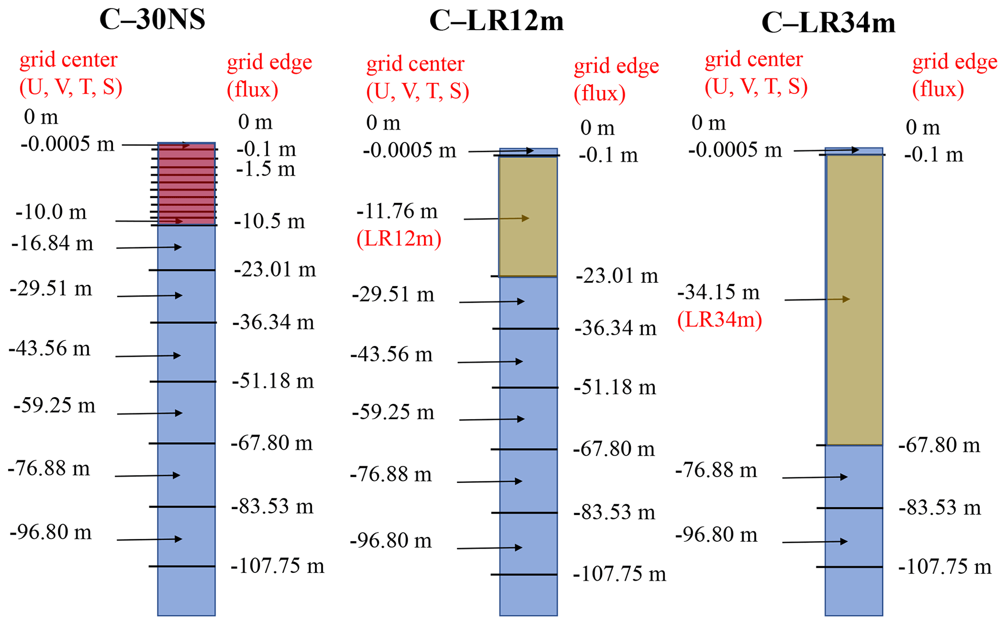
Figure A1 Diagram showing the vertical grid within 107.8 m in C–30NS, C–LR12m, and C–LR34m. The model is as thick as 107.8 m and with several layers between the surface and model bottom. C–LR12m (31 vertical layers) and C–LR34m (28 vertical layers) have a first layer with grid centers of 12 and 34 m, respectively, but have the same vertical discretization as in the control experiment (C–30NS, 41 vertical layers) below the first layer.

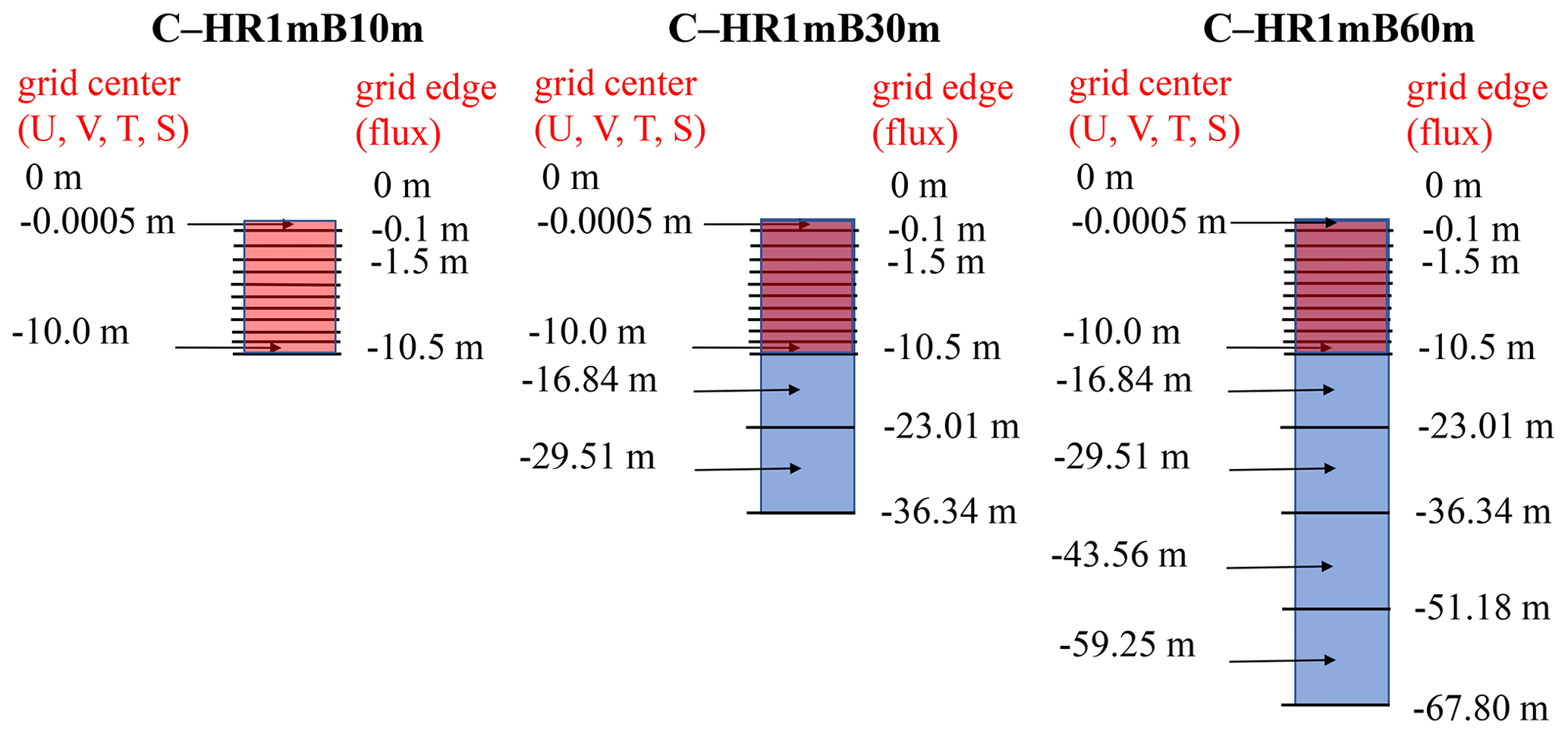
Figure A2 Diagrams showing the vertical grids in C–HR1mB10m, C–HR1mB30m, and C–HR1mB60m. The model bottoms are 10, 30, and 60 m, respectively, unless the seabed is shallower than the above depth.