the Creative Commons Attribution 4.0 License.
the Creative Commons Attribution 4.0 License.
 | 12 Jul 2022
Assimilation of GPM-retrieved ocean surface meteorology data for two snowstorm events during ICE-POP 2018
Xuanli Li
Jason B. Roberts
Jayanthi Srikishen
Jonathan L. Case
Walter A. Petersen
Gyuwon Lee
Christopher R. Hain
As a component of the National Aeronautics and Space Administration's (NASA's) Weather Focus Area and Global Precipitation Measurement (GPM) Ground Validation participation in the International Collaborative Experiments for the PyeongChang 2018 Olympic and Paralympic Winter Games' (ICE-POP 2018) field research and forecast demonstration programs, hourly ocean surface meteorology properties were retrieved from the GPM microwave observations for January–March 2018. In this study, the retrieved ocean surface meteorological products – 2 m temperature, 2 m specific humidity, and 10 m wind speed – were assimilated into a regional numerical weather prediction (NWP) framework. This explored the application of these observations for two heavy snowfall events during the ICE-POP 2018, on 27–28 February and 7–8 March 2018. The Weather Research and Forecasting (WRF) model and the community Gridpoint Statistical Interpolation (GSI) were used to conduct high-resolution simulations and data assimilation experiments. The results indicate that the data assimilation has a large influence on surface thermodynamic and wind fields in the model initial condition for both events. With cycled data assimilation, a significantly positive influence of the retrieved surface observation was found for the March case, with improved quantitative precipitation forecasts and reduced errors in temperature forecasts. A slightly smaller yet positive impact was also found in the forecast for the February case.
- Article
(11760 KB) - Full-text XML
- BibTeX
- EndNote


Cold season storms make great contributions to the global water cycle and influence local water supplies for household, agriculture, and manufacturing uses. In addition, winter sports tourism involving outdoor activities such as skiing, snowboarding, snowmobiling, ice fishing, etc., is a large market segment for mid to high-latitude regions. On the other hand, hazardous winter weather, including blizzards, ice storms, freezing rains, and heavy snow, often disrupts transportation; affects outdoor activities; causes delays and closures of airports, government offices, schools, and businesses; produces widespread and extensive property damage and loss of electricity; and presents hazards to human health, even the loss of life (Changnon, 2003, 2007; Call, 2010; FEMA, 2021; Smith, 2020).
Accurate and timely forecasts of the onset, duration, intensity, type, and spatial extent of precipitation are a major challenge in winter weather forecasting (Garvert et al., 2005; Ralph et al., 2005, 2010; Novak and Colle, 2012). These are especially important factors for providing support to ensure the success of highly weather-sensitive venues, such as the winter Olympic and Paralympic Games that were held in South Korea during February and March 2018. Many factors can contribute to the development of winter precipitation, including synoptic forcing (e.g., warm advection, differential vorticity advection), strong baroclinicity in the presence of moisture sources (e.g., near coastlines), and large-scale environmental instability in the warm sector of a mid-latitude cyclone. For regions that contain complex terrain in proximity to large bodies of water (such as the Korean Peninsula), local circulations and air–sea interactions also play important roles in determining the phase and amount of precipitation (Niziol et al., 1995; Kain et al., 2000; Schultz et al., 2002; O'Hara et al., 2009; Alcott and Steenburgh, 2010; Novak and Colle, 2012; Schuur et al., 2012; Novak et al., 2014; Roller et al., 2016).
In the Korean Peninsula, the weather and climate regimes during the winter months are largely driven by the seasonal reversal of winds across eastern Asia and the western North Pacific Ocean, from predominantly south/south-westerlies during the boreal summer months to north/north-easterlies during boreal winter (Chang et al., 2006). The east Asian winter monsoon (EAWM) months are considered between November and March, and largely drive the temperature and precipitation patterns across Korea. The dominant weather features associated with the EAWM consist of a strong low pressure in the Aleutian region of Alaska, a cold-core Siberian–Mongolian High, and low-level northeasterly winds along the Russian east coast. Variability in the strength of the EAWM (described in Zhang et al., 1997) has been correlated to El Niño/Southern Oscillation phase (where La Niña [El Niño] corresponds to stronger [weaker] EAWM), and snowpack anomalies during the autumn/winter across Siberia, eastern Russia, and northeastern China (positive snowpack anomalies lead to stronger EAWM). A stronger EAWM corresponds to strong Aleutian lows, Siberian–Mongolian highs, a stronger subtropical jet stream across eastern Asia, and deeper troughs in eastern Asia (Chang et al., 2006). Lee et al. (2010) found that, contrary to expectations, storm track activity is reduced during stronger EAWM and increased during weaker EAWM years.
Due to the prevailing EAWM regime, the Korean Peninsula can feel the effect of severe winter weather in the form of rapidly deepening mid-latitude cyclones and occasional cold surges from the Siberian–Mongolian semi-permanent high. Bomb cyclogenesis is most common along the Japanese coastline, but because of the Korean Peninsula's proximity to the Yellow Sea (west) and the Sea of Japan (east), strong baroclinicity can develop between the cold continental polar air over land and the warmer waters that provide abundant fluxes of heat and moisture into the atmosphere. Therefore, the rapid deepening of cyclones can also occur in the vicinity of the Korean Peninsula. In their satellite-era climatology of east Asian extratropical cyclones, Lee et al. (2020) showed that the Korean Peninsula feels the influence of extratropical cyclones originating in three preferred regions, Mongolia, East China, and the Kuroshio current along the southern/eastern coast of Japan. Using reanalysis data back to 1958, Zhang et al. (2012) found similar results in terms of the common cyclogenesis regions affecting eastern Asia. Yoshiike and Kawamura (2009) found that while bomb cyclogenesis occurred slightly more frequently during weak EAWM years, it was more concentrated along the south-eastern Japanese coast during strong EAWM, owing to larger heat fluxes over the Kuroshio current.
Locally intense mesoscale cyclones have also been documented across the Sea of Japan, developing in response to polar outbreaks over the warmer waters in conjunction with the complex terrain along and north of the Korean Peninsula. Tsuboki and Asai (2004) describe the process of strong convergence forming east of the Korean Peninsula, with substantial sensible and latent heating from the Sea of Japan, leading to the formation of these mesoscale cyclones. Intense Sea of Japan cyclones can cause substantial wave activity and subsequent coastal damage along the east coast of Korea (Lee and Yamashita, 2011; Oh and Jeong, 2014; Mitnik et al., 2011) in addition to significant snowfalls across Korea. Clearly, an accurate representation of air–sea interactions in NWP models is important when forecasting the impacts of winter cyclones and accompanying heavy snowfalls across the Korean Peninsula.
Numerous studies showed that in situ and remote-sensed observations for surface conditions and the upper atmosphere can provide a better description for both storm-scale processes and large-scale environments, leading to improved precipitation forecasts (Zupanski et al., 2002; Cucurull et al., 2004; Zhang et al., 2006; Fillion et al., 2010; Hartung et al., 2011; Hamill et al., 2013; Salslo and Greybush, 2017; English et al., 2018; Zhang et al., 2019). In South Korea, data assimilation also indicated significant benefits for winter forecasts (Kim et al., 2013; Kim and Kim, 2017; Yang and Kim, 2021). For example, Kim et al. (2013) demonstrated the assimilation of the conventional surface and upper air observations, aircraft, and multiple satellite observations located upwind or in the vicinity of the Korean Peninsula into the Korea Meteorological Administration (KMA) Unified Model. The results showed large decreases in the forecast error for the 24, 36, and 48 h forecasts of a strong winter storm event.
It is indicated that better representation of the air–sea interaction from the ocean can provide benefits to the forecasts of winter storms occurring in downstream regions. For example, Peevey et al. (2018) showed a significant reduction in forecast error when dropsonde observations over the Pacific Ocean were assimilated for winter storms in the western United States. Therefore, it is of great interest to assimilate the observations over oceans surrounding the Korean Peninsula and examine their impacts on winter storms affecting the Peninsula. However, regular observations over these oceans are limited to only a few buoys, satellite observations, and retrieved products that can provide broad spatial coverage, thus, regular revisits of data-sparse regions may be of substantial benefit.
In support of the International Collaborative Experiments for the PyeongChang 2018 Olympic and Paralympic Winter Games' (ICE-POP 2018) field campaign, special efforts were made to generate a set of near-surface ocean meteorology conditions (2 m air temperature, 2 m specific humidity, and 10 m wind speed) using the Global Precipitation Measurement (GPM) microwave observations from January to March 2018. In the satellite-based surface flux community (e.g., see Curry et al., 2004), significant efforts have been undertaken to estimate the near-surface meteorology from passive microwave observations to support the development of turbulent flux estimates from space. In particular, efforts have been made to estimate 2 m air temperature and humidity (e.g., Jackson et al., 2006; Roberts et al., 2010; Tomita et al., 2018) to complement long-standing wind speed estimates from microwave observation. However, the aforementioned efforts have almost explicitly focused on the large-scale production of the fluxes for climatological analyses with long latencies. On the other hand, the surface retrieval products essentially provide similar measurements to those of buoys and generally, with accurate performance. There is a long heritage of assimilating ocean surface buoy measurements within a data assimilation framework, but there has been little effort focused on assimilating the surface retrievals. This is partly due to a lack of a real-time availability of these estimates and partly due to the focus on a radiance-based assimilation system. The ICE-POP 2018 campaign provided a unique opportunity with near real-time passive microwave estimates of surface meteorology and a heavily observed regional environment to test the potential impact of assimilating widespread observations of near-surface meteorology. In this research, we introduced this particular surface meteorology dataset retrieved from the GPM microwave observation and explored the assimilation of this dataset using case studies with two snowstorm events occurred during the ICE-POP 2018 period. The objectives of the current research are to demonstrate the influence of this dataset and to examine whether or not the assimilation of this dataset is able to improve the forecasts of heavy snowstorms in the Korean Peninsula. Our focus herein emphasizes the impacts of assimilation of the surface meteorology data on corresponding model fields and downstream forecast skill. Follow-on efforts will examine more of the detailed physical processes (e.g., ocean evaporation and water and energy budget analyses) through which the assimilation impacts are forecast.
2.1 GPM-retrieved ocean surface meteorology data for ICE-POP 2018
The ICE-POP 2018 field campaign was led by the KMA as a component of the World Meteorological Organization's (WMO's) World Weather Research Program (WWRP) Research and Development and Forecast Demonstration projects (RDP/FDP) in order to enhance the capability of convective-scale numerical weather prediction modeling and to improve the understanding of high impact weather systems. The field campaign took place during the Winter Olympics (February–March) of 2018 in support of the 23rd Olympic Winter Games held in PyeongChang, Korea on 9–25 February and during the 13th Paralympic Winter Games from 9–18 March 2018. It ran in real time to provide guidance for forecasters during the Olympic Games. The focus of ICE-POP 2018 was to collect observations to measure the physics of heavy snow over the complex terrain in the PyeongChang region of South Korea and to improve the predictability of winter storm forecasting. During ICE-POP 2018, remote sensing and in situ observations were collected with an intensive instrument network, including enhanced surface weather stations, radiosondes, and wind profilers. Cloud and precipitation processes were observed with four KMA S-band Doppler radars and an X-band Doppler radar, National Aeronautics and Space Administration (NASA) Dual-frequency Dual-polarimetric Doppler Radar (D3R), lidar, Precipitation Imaging Packages (PIP), Micro Rain Radars (MMR), microwave radiometers, Parsivel disdrometers, etc. An aircraft and a marine weather-observing ship were also deployed during the campaign (as detailed in Petersen et al., 2018). Besides the remote-sensing data collected by NASA and KMA, high resolution ground-based in situ observation was also available. The South Korean Surface Analysis (SKSA) is a product interpolated from the observations collected by the enhanced Automatic Weather Station (AWS) network in South Korea using a newly developed radial basis function (Ryu et al., 2020). This dataset provides the surface temperature, moisture, wind, pressure, and precipitation amount over continental South Korea in a Lambert conformal conic projection with a 1 km horizontal spatial resolution and 10 min time interval. This dataset was used in this study to evaluate the model performance and the impact of the data assimilation.
The GPM is an international mission led by NASA and the Japanese Aerospace Exploration Agency (JAXA). The GPM contains a network of the GPM “core” satellite and eight other constellation radiometers (e.g., Special Sensor Microwave Imager/Sounder (SSMIS), Advanced Microwave Scanning Radiometer 2 (AMSR-2), and Microwave Humidity Sounder (MHS)). From the core satellite, partner research, and operational microwave sensors, GPM provides unified precipitation retrievals for real time and near real time over a large fraction of the globe (Hou et al., 2014; Skofronick-Jackson et al., 2017). As part of the NASA Weather Focus Area and GPM support of the ICE-POP 2018 program, near real-time ocean surface turbulence flux retrievals were produced based on Roberts et al. (2010), using intercalibrated passive microwave radiometer observations that were produced in support of the Integrated Multi-SatellitE Retrievals for GPM (IMERG) precipitation product (Berg et al., 2018). While intended to support precipitation estimations, these brightness temperatures are also capable of supporting the estimation of marine surface meteorology – wind speed, sea surface temperature, air humidity, and temperature – that are required to estimate surface turbulent fluxes. In this paper, we are interested in these near-surface atmosphere conditions rather than the fluxes. The microwave imagers provide information on near-surface winds, moisture, and temperature associated with the 10, 18.7, 23.8, 36.5, and 891 GHz vertical and horizonal polarized microwave channels. These channels are used together with an a priori estimate of sea surface temperature from the NCEP real-time global high-resolution (∘) sea surface temperature (RTG-SST) product to retrieve 10 m wind speed, 2 m specific humidity, 2 m air temperature, and sea surface temperatures. The retrieval algorithm is based on a single-layer neural network following Roberts et al. (2010). A large training dataset of standardized ocean buoy observations collocated within 1 h and 25 km of observations with each microwave sensor was developed. These data were broken into a training and set-aside independent validation dataset with a 60 % and 40 % split, respectively. For training data, the data were split into a training and cross-validation dataset with a 70 % and 30 % split. These retrieved parameters were then used to estimate the surface turbulent fluxes through an application of the Coupled Ocean–Atmosphere Response Experiment (COARE) 3.5 (Edson et al., 2013) bulk flux algorithm. Compared to the independent validation data, the root mean square (RMS) uncertainties are assessed at 1.1 g kg−1, 0.9 K, and 1.2 m s−1 for surface humidity, temperature, and wind speed, respectively, based on the mean statistics computed for the GPM Microwave Imager (GMI), Advanced Microwave Scanning Radiometer 2 (AMSR2), and the Special Sensor Microwave Imager/Sounder (SSMIS) microwave imagers for which retrievals were developed. The retrievals were essentially unbiased against the validation observations.
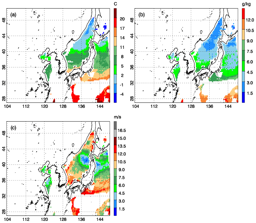
Figure 1A sample plot of the GPM-retrieved ocean surface meteorology data for (a) 2 m temperature (∘C), (b) 2 m specific humidity (g kg−1), and (c) 10 m horizontal wind speed (m s−1) at 09:00 UTC 7 March 2018.
The GPM-retrieved surface observations are generally available over the oceans around the Korean Peninsula within 1 h from 00:00, 06:00, 09:00, 12:00, 18:00, and 21:00 UTC on 7–8 March 2018. For 27–28 February, the retrieved data are typically available within 1 h from 00:00, 06:00, 09:00, 15:00, 18:00, and 21:00 UTC. The coverage of the retrieval product varies with time due to the geolocation of the microwave imager swaths. At most of the abovementioned times, observations typically cover ∼ 27–50∘ N over the Sea of Japan and the western North Pacific Ocean to the east of Japan. At 09:00, 18:00, and 21:00 UTC, the Bohai Sea and Yellow Sea to the west of the Korean Peninsula are usually observed or partly observed. Figure 1 shows an example of GPM-retrieved 2 m temperature, 2 m specific humidity, and 10 m wind speed at 09:00 UTC 7 March 2018, when the observations cover the west part of the Bohai and Yellow seas, most parts of the Sea of Japan, and the western North Pacific Ocean. At this time, cold (< −1 ∘C) and dry (< 3.0 g kg−1) air was observed at latitude above 44∘ N and warm (> 17 ∘C) and moist (> 10.5 g kg−1) air at latitude lower than 30∘ N. Observed surface temperature ranges from −7–23 ∘C and surface humidity from 0–13.5 g kg−1 over the model domain. Surface wind speed is found between 0–18 m s−1. Low wind centers appeared near the northern coast of Japan, one in the central east Sea of Japan, and the other one in the western North Pacific Ocean.
2.2 Data assimilation system and numerical experiments
Two heavy snowstorms affecting the Korean Peninsula and the ICE-POP field domain on 27–28 February and 7–8 March 2018 were selected for the case studies. Figures 2 and 3 summarize the evolution of surface features for the two case studies. In both instances, a surface low pressure developed to the south and southwest of the Korean Peninsula and tracked to the northeast, passing along or just off the South Korean southern coast. This placed the mountainous portions of South Korea, including the Olympics/Paralympics venue, in the favorable northwestern quadrant of the surface low for heavy snowfall. During the 27–28 February snowstorm, a closed 1005 hPa low was situated just off the eastern China coastline at 00:00 UTC 28 February to the southwest of the Korean Peninsula with another closed low over northeastern China at 1008 hPa (Fig. 2a). The southern low experienced substantial deepening as it tracked northeastward over the next 24 to 36 h, reaching extreme southern South Korea by 12:00 UTC 28 February at 994 hPa intensity (Fig. 2b), the central Sea of Japan by 00:00 UTC 1 March at 987 hPa and absorbing the northern low by this time (Fig. 2c), and then into northern Japan by 12:00 UTC 1 March at 974 hPa minimum central pressure (Fig. 2d). The 28 February was the warmer of the two snowstorms, with most snow accumulation confined to the mountainous terrain along the Korean east coast, including the Olympics venue where the storm-total snow accumulations of ∼ 40 cm were observed (not shown). Gehring et al. (2020) analyzed the warm conveyer belt and microphysical characteristics of this heavy precipitation event using datasets from the ICE-POP 2018 field campaign.
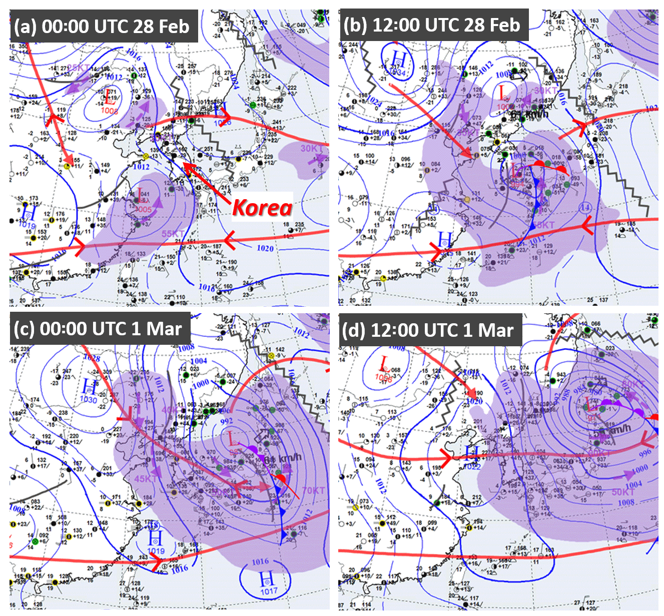
Figure 2Eastern Asia regional surface meteorological analyses by the KMA at 12-hourly intervals, valid at (a) 00:00 UTC 28 February, (b) 12:00 UTC 28 February, (c) 00:00 UTC 1 March, and (d) 12:00 UTC 1 March 2018.

Figure 3Same as Fig. 2, except valid at (a) 12:00 UTC 7 March, (b) 00:00 UTC 8 March, (c) 12:00 UTC 8 March, and (d) 00:00 UTC 9 March 2018.
Temperatures were slightly colder during the 7–8 March event, resulting in a more widespread snowfall across the southern and eastern Korean Peninsula within the mountains and at lower elevations. Following the general synoptic snows, a surge of stronger north/northeasterly low-level winds off the Sea of Japan affected the Korean east coast and eastern mountains, leading to enhanced residual precipitation and strong orographic uplift (not shown). The 7–8 March extratropical cyclone began as a weak, open wave at 12:00 UTC 7 March (Fig. 3a), then deepened to a 1010 hPa closed low to the southeast of the Korean Peninsula at 00:00 UTC 8 March (Fig. 3b). The cyclone slowly strengthened over the next 24 h to 1004 hPa over the eastern Sea of Japan by 12:00 UTC 8 March (Fig. 3c) and then to 1003 hPa as it tracked northeastward into northern Japan by 00:00 UTC 9 March (Fig. 3d). An elongated meridional trough extended out of the low pressure center across much of Japan, resulting in a long fetch of north/northeasterly low-level winds across the Sea of Japan that affected the east coast of Korea during 8 March.
The Advanced Research Weather Research and Forecasting (WRF ARW; Powers et al., 2017) model was used to conduct the regional simulations for the two events. The snowstorms were simulated using three nested domains with a horizontal resolution of 9, 3, and 1 km and 62 vertical levels as illustrated in Fig. 4. The model physics options include the Goddard long-wave and shortwave radiation schemes (Chou and Suarez, 1999), Grell–Freitas cumulus parameterization (Grell and Freitas, 2014), Mellor–Yamada–Janjic (MYJ) PBL schemes (Janjic, 1994), Morrison's double-moment microphysical scheme (Morrison et al., 2009), and the unified Noah land-surface model (Chen and Dudhia, 2001). The cumulus parameterization was only used for the outer 9 km resolution domain.
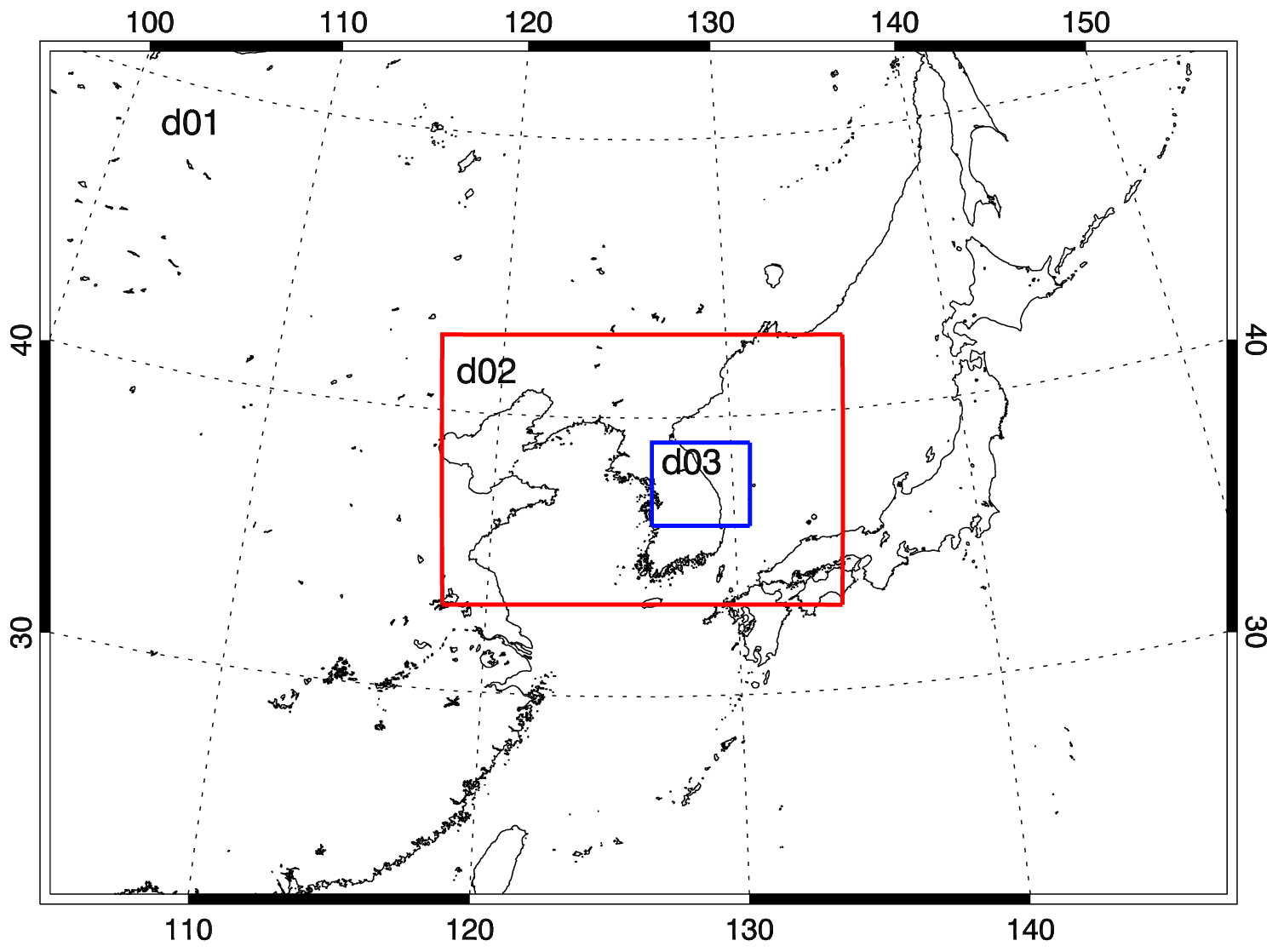
Figure 4WRF model domain configuration.
In the present study, the community Gridpoint Statistical Interpolation (GSI; Wu et al., 2002) v3.6 system was used to assimilate the GPM-retrieved ocean surface meteorology data. The GSI system was initially developed by the NCEP Environmental Modeling Center (EMC) and is currently maintained and supported by the National Oceanic and Atmospheric Administration (NOAA) Development Testbed Center (DTC; Hu et al., 2016). The GSI is built in physical space for a unified, flexible, and efficient modular system for multiple parallel computing environments and has been implemented real time into both global and regional data assimilation (Wu, 2005; De Pondeca et al., 2007; Kleist et al., 2009). The community GSI is functionally equivalent to the operational version used in NCEP. The system readily incorporates multiple types of observational data, including conventional data, radar, satellite radiance, and retrieved products.
The GSI system is a 3-dimensional variational (3DVAR) data assimilation system (more detailed description in Wu et al., 2002). In GSI, the 3DVAR cost function J is defined by the following equation:
where x is the analysis increment (xa−xb), xa is the analysis fields, xb is the background fields, Jc is the constraint terms, B is the background error covariance matrix for analysis control variables, is the observation innovation, R is the observational error covariance matrix, and H represents a transformation operator from the control variables to the observations. The control variables in GSI include the stream function, unbalanced velocity potential, unbalanced virtual temperature, unbalanced surface pressure, and pseudo relative humidity. The background error covariance is an important factor for a successful data assimilation. The GSI package comes with pre-computed files for B. To obtain a more accurate regional data assimilation result, we used the “gen_be” package in the WRF Data Assimilation (WRFDA) system to compute a domain-specific B using the “NMC method” (Parrish and Derber, 1992), with 1 month of WRF 24 and 12 h forecasts for all model domains. The B matrix provides model error statistics, including the vertical and horizontal length scales and regression coefficients for the control variables.
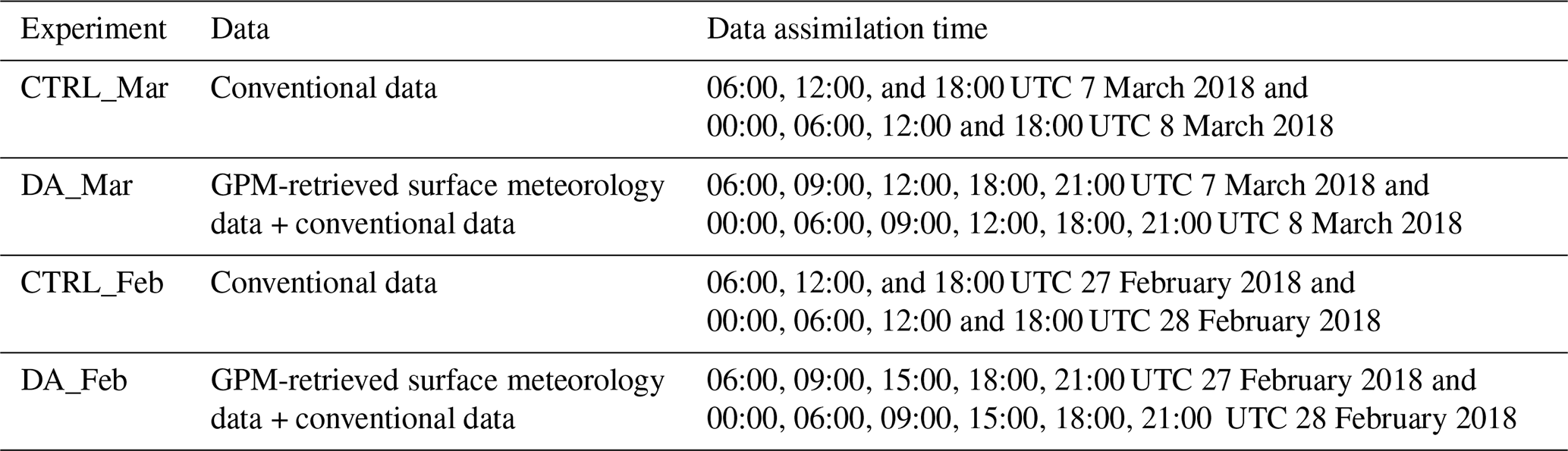
Table 1 lists the numerical experiments and corresponding data assimilation activities preformed for the two cases. Two different numerical experiments were conducted for each snowstorm event. For the 7–8 March case, the control experiment (CTRL_Mar) assimilates the conventional PREPBUFR observations every 6 h using the PREPBUFR data obtained from the National Center for Atmospheric Research (NCAR) Research Data Archive (available at https://rda.ucar.edu/datasets/ds337.0/, last access: 7 July 2022). The conventional data refer to the global surface and upper-air observation operationally collected by the National Center for Environmental Prediction (NCEP), which includes surface, marine surface, radiosonde, pibal and aircraft reports from the Global Telecommunications System (GTS), profiler, United States radar-derived winds, SSM/I oceanic winds and total precipitable water retrievals, and satellite wind report data from the National Environmental Satellite Data and Information Service (NESDIS). Another experiment, DA_Mar, assimilates the GPM-retrieved ocean surface temperature, specific humidity, and wind speed observations besides the conventional PREPBUFR data. As shown in Table 1, a cycled assimilation of the GPM-retrieved ocean surface meteorology data was performed at 06:00, 09:00, 12:00, 18:00, and 21:00 UTC for 7 March and 00:00, 06:00, 09:00, 12:00, 18:00, and 21:00 UTC for 8 March, based on the availability of the retrieval product. Both experiments began at 00:00 UTC 7 March 2018 and ended at 00:00 UTC 9 March 2018. For both experiments, the initial and boundary conditions of the WRF background field were interpolated from the 0.5∘ resolution Global Forecast System (GFS) analysis. For the 27–28 February 2018 event, CTRL_Feb and DA_Feb were conducted with settings similar to CTRL_Mar and DA_Mar, respectively. Both experiments started at 00:00 UTC 27 February 2018 and ended at 00:00 UTC 1 March 2018. For DA_Feb, the GPM-retrieved ocean surface meteorology data were assimilated at 06:00, 09:00, 15:00, 18:00, and 21:00 UTC for 27 February and 00:00, 06:00, 09:00, 15:00, 18:00, and 21:00 UTC for 28 February 2018.
In this section, the numerical experiments with and without the assimilation of the GPM-retrieved surface products were compared with the observations collected for the 7–8 March and 27–28 February snowstorm cases. The impact of the data on initial conditions and short-term forecasts are examined.
3.1 Case study for the 7–8 March snowstorm event
In order to illustrate the overall distribution of the GPM-retrieved surface observations and the difference from the background, Fig. 5a–c shows the scatterplot of 2 m temperature, 2 m specific humidity, and 10 m wind speed observations, with respect to the departures between the observed values and WRF background (i.e., a positive departure represents a higher value in observation than the model). As a pre-process step before data assimilation, outliers with a magnitude of surface temperature departure > 6 ∘C, specific humidity departure > 4 g kg−1, or wind speed departure > 9 m s−1 were removed. An examination of the location of the data used for the two cases indicated that a larger portion of the observational data were located at the south part of the Sea of Japan and western North Pacific Ocean than the north part. The probability density functions (PDF) of the departures of 2 m temperature, 2 m specific humidity, and 10 m wind speed are shown in Fig. 5d–f. An apparent skewness to the positive side is shown in the PDF of the surface temperature departure (Fig. 5d), with a skewness value of 0.36 ∘C. For surface-specific humidity, the departure shows a narrower spread with most of the values ranging from −2 to 2 g kg−1. The PDF of the surface-specific humidity departure skews to the negative side with a skewness of −0.48 g kg−1. This indicates a generally colder model atmosphere with higher specific humidity at ocean surface in the WRF background when compared to the observations. For surface wind speed, most of the departure values were within −5 and 5 m s−1, with a skewness of 0.33 m s−1, respectively.
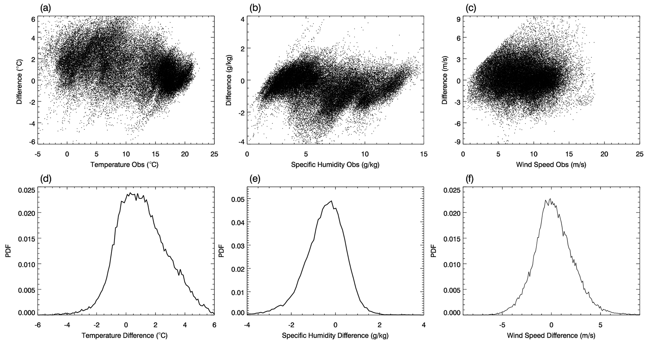
Figure 5Scatterplot for GPM-retrieved observation vs. the departure between the observation and the model background for (a) 2 m temperature (∘C), (b) 2 m specific humidity (g kg−1), and (c) 10 m horizontal wind speed (m s−1) from all available data during the data assimilation time windows for the two case studies. The probability density function (PDF) of the (d) 2 m temperature departure, (e) 2 m specific humidity departure, and (f) 10 m horizontal wind speed departure with a bin width of 0.1.
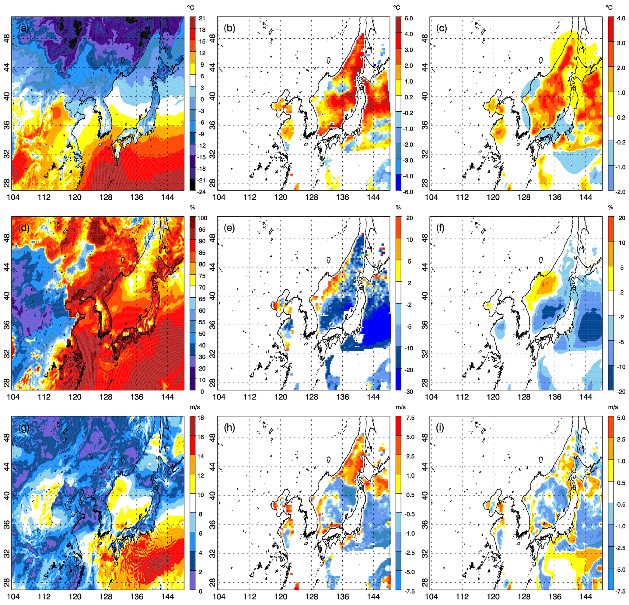
Figure 6WRF model background for (a) 2 m temperature (∘C), (d) 2 m relative humidity (%), and (g) 10 m horizontal wind speed (m s−1), difference between observation and model background for (b) 2 m temperature, (e) 2 m relative humidity, and (h) 10 m horizontal wind speed, and difference between data assimilation analysis and the background for (c) 2 m temperature, (f) 2 m relative humidity, and (i) 10 m horizontal wind speed at 09:00 UTC 7 March 2018.
Through data assimilation, the GPM-retrieved surface observation directly influences the thermodynamic and wind fields of the WRF initial condition. Figure 6 displays the surface condition of the 7–8 March case before and after the data assimilation cycle at 09:00 UTC 7 March 2018. Since specific humidity is not one of the GSI control variables and is a function of the temperature and water vapor mixing ratio, the observed specific humidity was converted into relative humidity in Fig. 6 for a more direct view on the data assimilation impact. The difference between the data assimilation analysis and the model background field (analysis–background, or “A–B”, the increment added to the model field after data assimilation in Fig. 6c, f, and i) was compared with the difference between the observation and the model background (observation–background, or “O–B”, in Fig. 6b, e, and h) to indicate the changes in surface temperature, relative humidity, and wind speed fields by data assimilation. Before the data were assimilated, the surface temperature in the model background was generally colder than the observation over the Bohai Sea, Yellow Sea, Sea of Japan, and a large part of the western North Pacific Ocean, which is reflected by the areas of positive O–B up to 6 ∘C (Fig. 6b). After data assimilation, an increase was made in surface temperature, indicated by positive A–B over the oceans (Fig. 6c), where positive O–B was found. From the plots for surface-relative humidity, it is indicated that the model background was more humid than the observation over most of the area of the Sea of Japan and the western North Pacific Ocean (Fig. 6e). After data assimilation, surface-relative humidity has decreased by up to 20 % over a large part of the western North Pacific Ocean and east Sea of Japan. Only at the west Sea of Japan, an increase in humidity (Fig. 6f) was created due to the positive O–B over the area (Fig. 6e). For surface wind speed, the background is apparently quieter at the northern Sea of Japan and the northern part of the western North Pacific Ocean, and generally higher than observations from the central to southern Sea of Japan and the western North Pacific Ocean, with a latitude below 40∘ N (Fig. 6h). After data assimilation, A–B generally agrees with the pattern shown in O–B (Fig. 6i). The root mean square difference (RMSD) was also calculated for O–B and A–B at locations where the observational data are valid. RMSD is 2.35 ∘C, 8.12 %, and 4.16 m s−1 for O–B in surface temperature, relative humidity, and wind speed, respectively. For A–B, RMSD is 1.36 ∘C, 4.01 %, and 1.83 m s−1, indicating an effective assimilation of the observational data was made to the WRF initial condition.
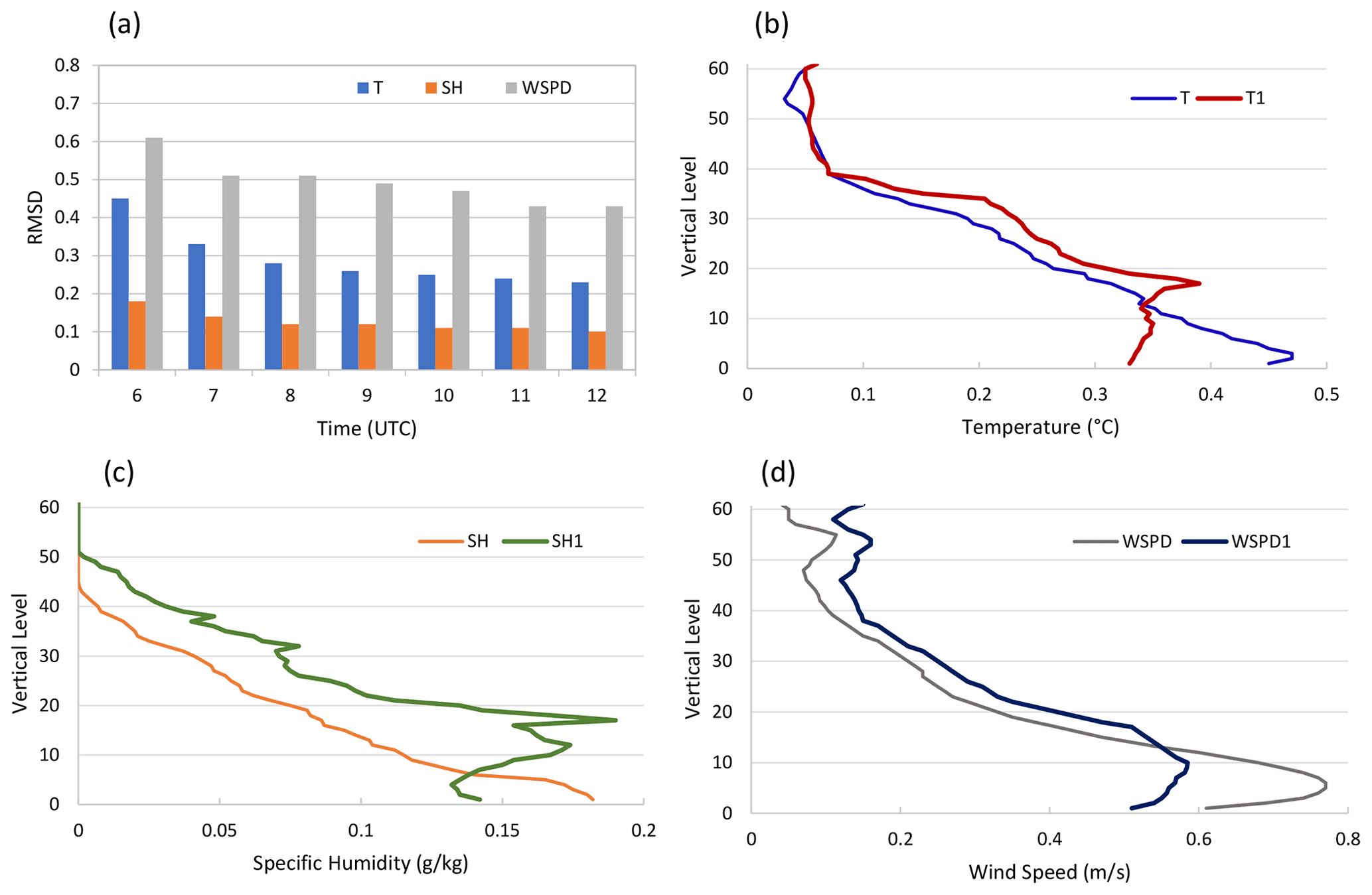
Figure 7(a) Root mean square difference (RMSD) between DA_Mar and CTRL_Mar for 2 m temperature (∘C), 2 m specific humidity (g kg−1), and 10 m horizontal wind speed (m s−1), calculated over the model domain from 06:00 UTC 7 March to 12:00 UTC 7 March 2018, and vertical profiles of RMSD for (b) temperature, (c) specific humidity, and (d) wind speed at 06:00 UTC (T, SH, and WSPD) and 07:00 UTC (T1, SH1, and WSPD1) 7 March 2018.
With the initial condition provided from data assimilation, the WRF forecast began. During the model integration, some of the changes in the initial condition were enhanced and some of the changes were reduced by the model dynamic adjustment. Therefore, it is important to understand how long and by how much the data impact will last in the model forecast. Figure 7a shows the RMSD in surface temperature, surface specific humidity, and surface wind speed between DA_Mar and CTRL_Mar, calculated over the entire model domain for 0–6 h forecast after the first data assimilation cycle conducted at 06:00 UTC 7 March 2018. At 06:00 UTC, domain-averaged RMSD is 0.45 ∘C, 0.18 g kg−1, and 0.61 m s−1 for surface temperature, specific humidity, and wind speed, respectively. After the first hour of integration, the RMSD showed a rapid decline to 0.33 ∘C, 0.14 g kg−1, and 0.51 m s−1, which is 27 %, 22 %, and 16 % reduction to the original values in the analysis. In the next 5 h of integration, these values dropped slowly to 0.23 ∘C, 0.10 g kg−1, and 0.43 m s−1, corresponding to 51 %, 55 %, and 70 % of the original values. This means a strong model adjustment occurred in the first hour of integration, followed by a slow spreading of the impact in the next few hours. By the end of the 6 h forecast, we can still see a large amount of impact retained in the model fields. Figure 7b–d provides the vertical profiles of RMSD of temperature, specific humidity, and wind speed calculated over the entire model domain to indicate how the higher vertical levels respond to the changes in the surface condition through model adjustment. Profiles T, Q, and WSPD represent the RMSD values at 62 model vertical levels at 06:00 UTC, and T1, Q1, WSPD1 are for 07:00 UTC 7 March 2018. After the 1 h time integration, Fig. 7b shows a large decrease in temperature RMSD at surface and low atmosphere. The RMSD decrease declined with height. In the mid-troposphere from the model level 13 (∼ 875 hPa) to 39 (∼ 550 hPa), an increase in temperature RMSD was found. A similar trend was also found in the RMSDs for specific humidity and wind speed. For specific humidity, Fig. 7c indicates the 07:00 UTC forecast has a smaller RMSD in the boundary layer below model level 7 (∼ 920 hPa) and a significantly larger RMSD at levels above it until level 50 (∼ 300 hPa). From 06:00 to 07:00 UTC, an apparent decrease in the wind speed RMSD was found (Fig. 7d) in the low atmosphere below model level 13 (∼ 875 hPa) and a consistent increase from the mid to upper-level.
Table 2Root mean square error (RMSE) for 2 m temperature (∘C) forecast over South Korea for difference experiments.
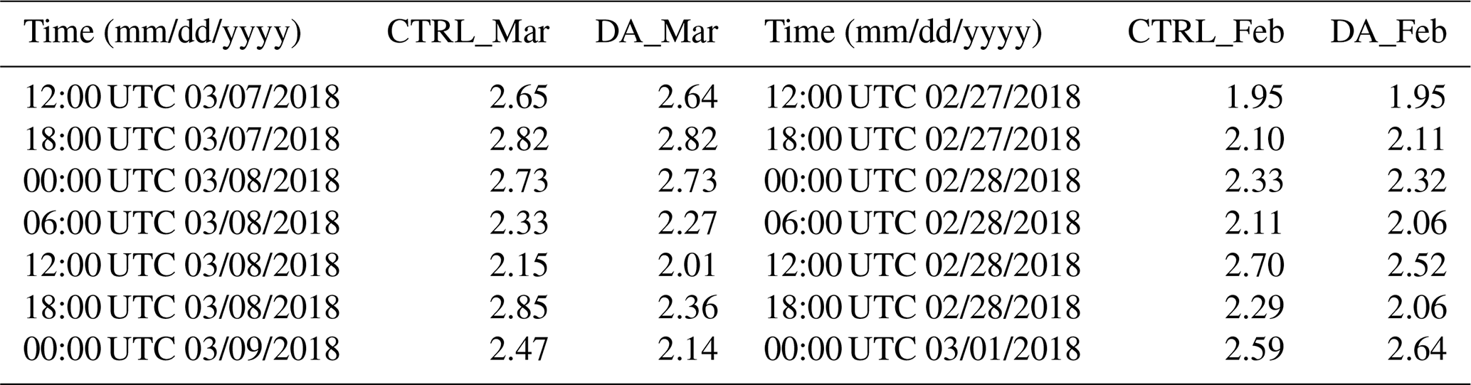
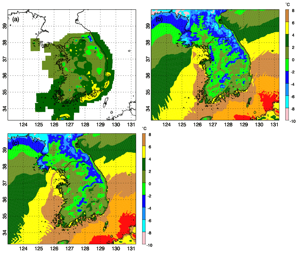
Figure 82 m temperature field (∘C) from (a) South Korean Surface Analysis, (b) CTRL_Mar, and (c) DA_Mar at 15:00 UTC 8 March 2018.
The impact of the cycled assimilation of the GPM-retrieved data on surface temperature forecast was examined with the root mean square error (RMSE) for 2 m temperature. The RMSE (Table 2) was calculated every 6 h across continental South Korea from 12:00 UTC 7 March to 00:00 UTC 9 March using the South Korean Surface Analysis as the reference dataset. From 12:00 UTC 7 March to 00:00 UTC 8 March, the RMSE values in DA_Mar were close to those in CTRL_Mar. After the seventh cycle of data assimilation at 06:00 UTC 8 March, RMSEs in DA_Mar were consistently smaller than CTRL_Mar. At the end of the model simulation time, surface temperature RMSE in DA_Mar was 2.14 ∘C, which is 0.33 ∘C lower than CTRL_Mar. Figure 8 shows an example of 2 m temperature from the South Korean Surface Analysis compared to CTRL_Mar and DA_Mar at 15:00 UTC 8 March 2018. Generally, surface temperature was around 0–4 ∘C at this time over South Korea, with a few warmer areas of 4–6 ∘C along the southeastern coast and Jeju Island. A colder temperature (−2 ∘C) was observed in the Taebaek Mountains over the northeastern tip of the country. Both CTRL_Mar and DA_Mar predicted colder temperatures than the observation over most areas of South Korea. This is especially apparent for regions with a higher topography, e.g., along the Taebaek Mountain range and the Sobaek Mountains. Compared to CTRL_Mar, DA_Mar produced a better forecast with much a smaller area, with a temperature below 0 ∘C and a warmer temperature along the Taebaek Mountains. The RMSE of 2 m temperature calculated at this time confirms the conclusion in Fig. 8, with 2.89 ∘C in CTRL_Mar and 2.03 ∘C in DA_Mar.
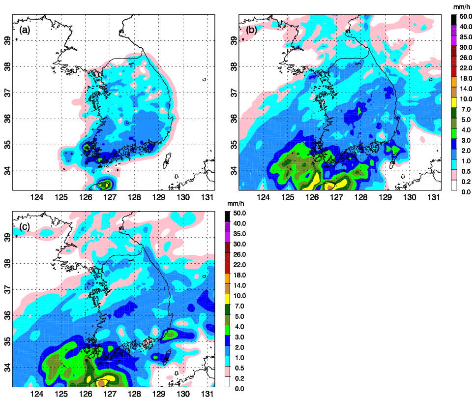
Figure 91 h precipitation (mm h−1) from (a) South Korean Surface Analysis, (b) CTRL_Mar, and (c) DA_Mar at 16:00 UTC 7 March 2018.
The impact of the GPM-retrieved ocean surface data on precipitation forecasts is shown in Fig. 9. The 1 h precipitation observed by the South Korean Surface Analysis at 16:00 UTC 7 March 2018 was compared to the results from CTRL_Mar and DA_Mar. At this time, light snowfall was broadly observed over northern to central South Korea. The storm started to produce heavier snowfall in the southern region, with > 3 mm h−1 in the southwestern tip of the Korean Peninsula and > 8 mm h−1 in Jeju Island. From Fig. 9b and c, it is indicated that the simulated storm in both DA_Mar and CTRL_Mar also produced light to moderate snowfall over most of the area of South Korea, with heavier precipitation over the southwest end of the Korean Peninsula. The pattern of precipitation in DA_Mar is very similar to CTRL_Mar. Strong precipitation was predicted in Jeju Island in both CTRL_Mar and DA_Mar. Compared to DA_Mar, CTRL_Mar produced an overall stronger precipitation, indicated by the larger area with a precipitation rate above 1 mm h−1 from central to southern South Korea. The threat score (TS) can provide a point-by-point evaluation of the precipitation forecast. TSs were calculated for continental South Korea at 16:00 UTC 7 March using the following equation, based on Xiao et al. (2005):
where C is the number of correct forecast events, F is the number of forecast events, and R is the number of observed events in South Korean Surface Analysis data. The TSs of CTRL_Mar are 0.62, 0.51, and 0.09 for threshold values of 1, 2, and 3 mm h−1, respectively. A more accurate precipitation forecast was produced by DA_Mar, with higher TSs of 0.77, 0.57, and 0.15, respectively.
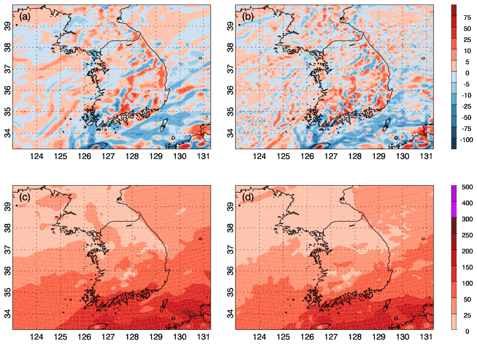
Figure 10Moisture flux divergence (× 10−4 g kg−1 s−1) for (a) CTRL_Mar and (b) DA_Mar, and magnitude of moisture transport (g kg−1 m s−1) for (c) CTRL_Mar and (d) DA_Mar for 925 hPa and at 16:00 UTC 7 March 2018.
Low-level moisture flux convergence is an important condition for precipitation in winter storms (Hartung et al., 2011). To better understand the mechanisms that lead to the improved precipitation forecast, the moisture flux divergence (Q⋅DIV) and moisture transport (Q⋅V) at 925 hPa from the CTRL_Mar and DA_Mar were compared in Fig. 10. In both CTRL_Mar and DA_Mar, strong moisture convergence regions (negative values in the color blue in Fig. 10a, b) correspond well with the snowfall (Fig. 9b, c) produced over the southern end of the Korean Peninsula and in the Korean Strait. The moisture convergence in both simulations was generally weak over the Korean Peninsula, which led to light to moderate snowfall over most of the area. A closer look at DA_Mar shows that data assimilation helped reduce moisture convergence near 128∘ E and 36∘ N (Fig. 10b), agreeing with the smaller area of precipitation > 2 mm h−1 (Fig. 9c). At the southern end of the Korean Peninsula, CTRL_Mar also produced stronger moisture convergence (Fig. 10a) compared to DA_Mar (Fig. 10b), which is consistent with the smaller precipitation amount in Fig. 9c. Similarly, low-level moisture transport in CTRL_Mar was characterized by larger values from central to southern South Korea (Fig. 10c) than DA_Mar (Fig. 10d). This is especially apparent in the region near 128∘ E and 36∘ N and along the southern coastline.
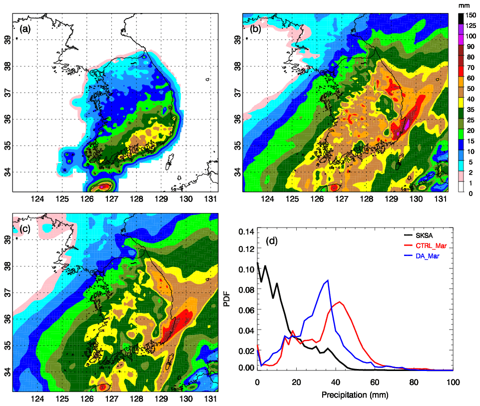
Figure 1124 h accumulated precipitation (mm) from (a) South Korean Surface Analysis, (b) CTRL_Mar, and (c) DA_Mar, from 06:00 UTC 7 March to 06:00 UTC 8 March 2018 and (d) the probability density function of 24 h accumulated precipitation.
The snowstorm moved northeastward and precipitation related to the system firstly appeared in the southwest end of South Korea at 08:00 UTC 7 March. A large amount of precipitation in South Korea was concentrated between 17:00 UTC 7 March and 00:00 UTC 8 March. In Fig. 11, 24 h accumulated precipitation from 06:00 UTC 7 March to 06:00 UTC 8 March was plotted for the observation and compared to the numerical experiments. From the South Korean Surface Analysis, there was over 20 mm snowfall produced in the southern provinces and cities, with over 40 mm snowfall along the coast in South Gyeongsang Province. As shown in Fig. 11b and c, both CTRL_Mar and DA_Mar overpredicted the precipitation, with > 15 mm precipitation covering almost the entire South Korea. Overestimation is especially apparent in CTRL_Mar, which predicted precipitation of > 40 mm over most of the area of the central and southern provinces. Heavy snowfall above 70 mm with the extreme value of 95 mm was predicted along the southeastern coast of Ulsan and the North Gyeongsang Province in CTRL_Mar. In comparison, DA_Mar predicted a much smaller area with precipitation exceeding 40 mm. In addition, the maximum precipitation was 82 mm, which was 13 mm lower than CTRL_Mar. The probability density function (PDF) of a 24 h precipitation amount was calculated with a bin size of 2 mm over South Korea, where the surface analysis data are available. It is shown that 13.5 % of the observed area in South Korea had light precipitation of 0–2 mm, 77.2 % of the entire area observed snowfall of < 20 mm, 19.6 % of the area had precipitation of 20–40 mm, and only 3.2 % of the area experienced precipitation of > 40 mm in the 24 h. Both CTRL_Mar and DA_Mar predicted a much lower percentage of area for light precipitation of 0–2 mm. In CTRL_Mar, the peak precipitation probability was predicted at 42 mm for 6.7 % of the area in South Korea. Snowfall of < 20 mm occurred at 19.3 % of the entire area, which is 57.9 % smaller than the observation. In CTRL_Mar, 20–40 mm snowfall was predicted for 39.4 % of the area, 19.8 % higher than the observed value. Precipitation of > 40 mm was generated for 41.3 % of the area, which is 38.1 % larger than the observation. DA_Mar performed better than CTRL_Mar with an overall lower precipitation amount. The peak precipitation probability was at 36 mm for 8.8 % of the area. Light snowfall below 20 mm was predicted for 23 % of the area, 20–40 mm snowfall for 60 % of the area, and > 40 mm for 17 % of the area, indicating less overprediction.
3.2 Case study for the 27–28 February snowstorm event
The above results indicate a positive impact of the GPM-retrieved surface meteorology data on the short-term forecast for the 7–8 March case. The assessment of the data assimilation results for the February case will be discussed in this section.
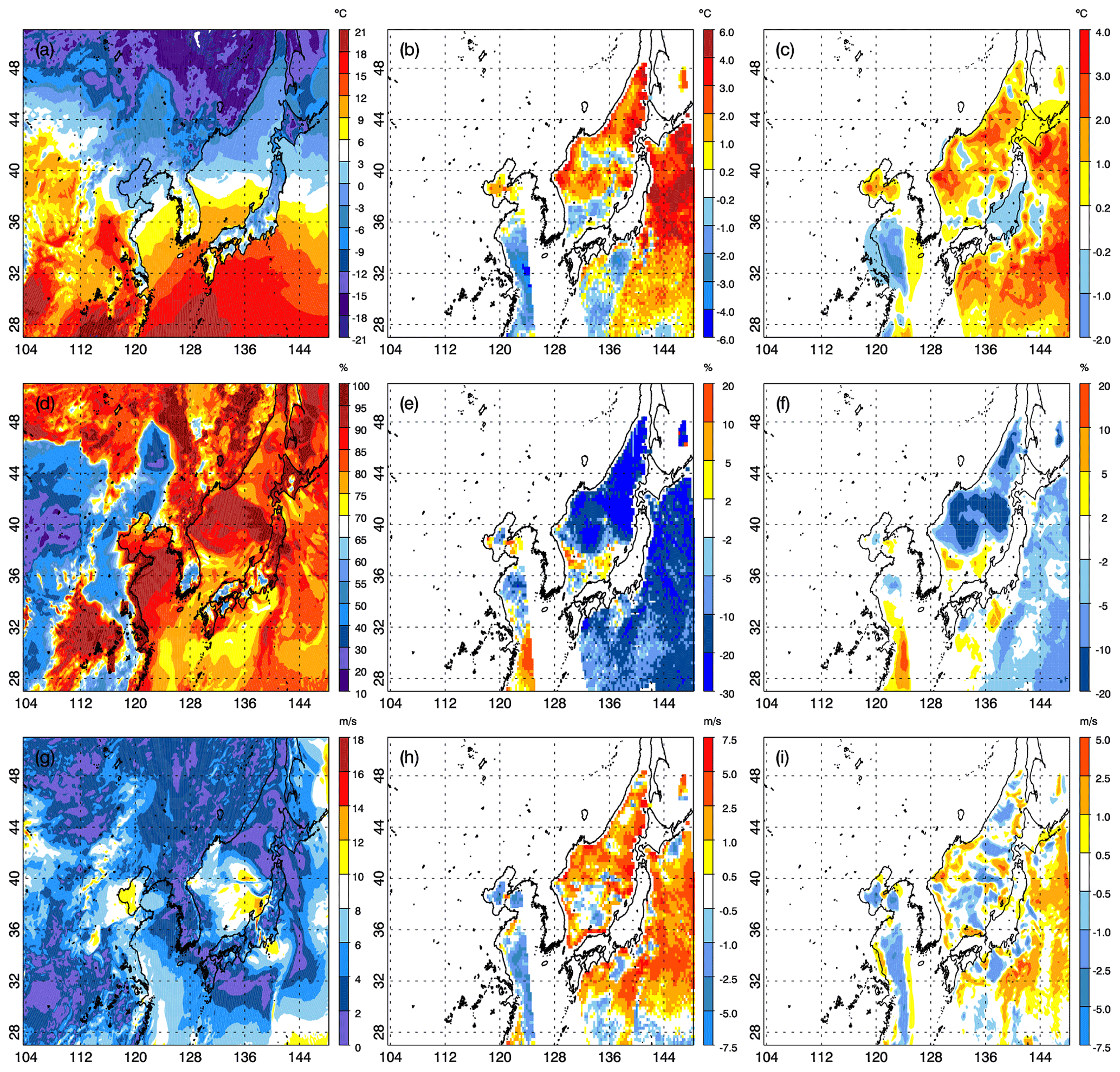
Figure 12WRF model background fields for (a) 2 m temperature (∘C), (d) 2 m relative humidity (%), and (g) 10 m horizontal wind speed (m s−1). The difference between GPM-retrieved observation and model background fields for (b) 2 m temperature, (e) 2 m relative humidity, and (h) 10 m horizontal wind speed. The difference between the data assimilation analysis and model background field for (c) 2 m temperature, (f) 2 m relative humidity, and (i) 10 m horizontal wind speed at 09:00 UTC 27 February 2018.
Figure 12 shows the surface temperature, relative humidity, and wind speed in the model background compared with O–B and A–B from DA_Feb at 09:00 UTC 27 February 2018. The GPM-retrieved observation at this time was available for a large part of the Bohai Sea and the eastern half of the Yellow and East China seas. The observation also covers the Sea of Japan and the western North Pacific Ocean. From Fig. 12b and e, the observed surface air was generally warmer in the Bohai Sea and colder and drier in the Yellow Sea than the model background. Over most of the regions in the Sea of Japan and the western North Pacific Ocean, the surface air was roughly > 1 ∘C warmer, but with lower relative humidity (by up to 30 %) than the model background. After data assimilation, positive increments in surface temperature were produced over the Bohai Sea, Sea of Japan, and the western North Pacific Ocean. In the Yellow Sea, negative increments in surface temperature and specific humidity were produced when the data were assimilated (Fig. 12c, f). A decrease in relative humidity was produced over the north and central Sea of Japan and most of the area of the western North Pacific Ocean. An increase in relative humidity was created over the southern Sea of Japan and in the East China Sea where more humid observation was found. For surface wind speed, the GPM-retrieved observation (Fig. 12h) was generally lower than the background over the Bohai Sea, Yellow Sea, and East China Sea, and higher in the Sea of Japan and western North Pacific Ocean. After the data assimilation, areas of decreased wind speed were found in the Bohai Sea, Yellow Sea, and East China Sea. Areas of increased surface wind speed have been produced in the western North Pacific Ocean with a magnitude up to 3.5 m s−1.
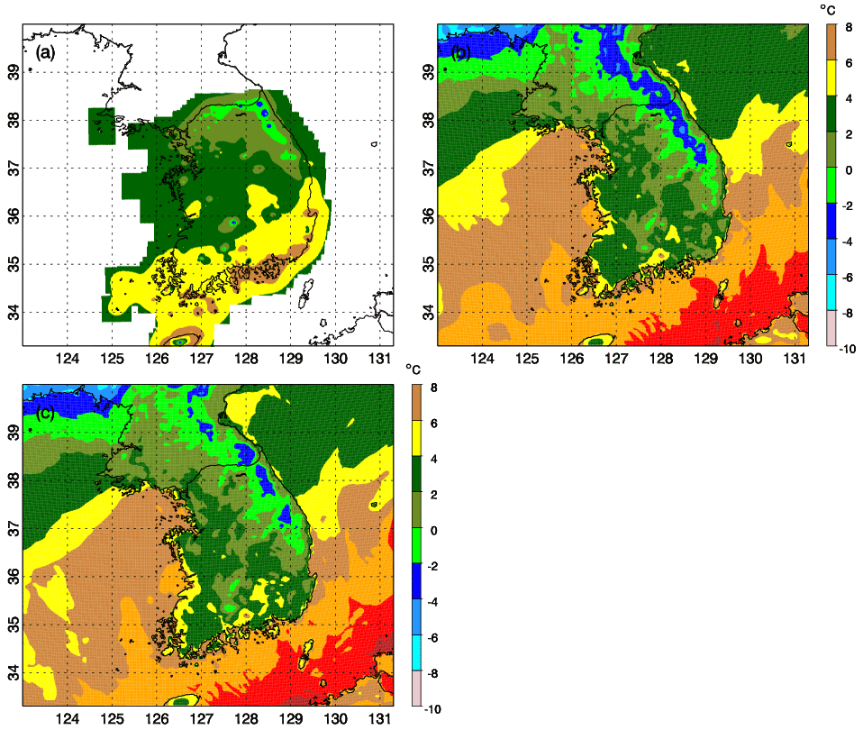
Figure 13The 2 m temperature field (∘C) from (a) South Korean Surface Analysis, (b) CTRL_Feb, and (c) DA_Feb at 18:00 UTC 28 February 2018.
Even though the positive impact of data assimilation was not as significant as the one shown in the March case, it is found that the surface temperature forecast was also improved for the 27–28 February event with data assimilation. The RMSEs of 2 m temperature calculated over South Korea from 12:00 UTC 27 February to 00:00 UTC 1 March 2018 were listed in Table 2. At 12:00 UTC 27 February, the RMSE in DA_Mar equals that in CTRL_Feb. From 18:00 UTC 27 February to 00:00 UTC 28 February, RMSEs in DA_Feb were very close to CTRL_Feb. From 06:00 to 18:00 UTC 28 February, DA_Feb provided smaller RMSEs than CTRL_Feb, implying a more skillful forecast. At the end of the simulation period, both CTRL_Feb and DA_Feb produced a larger RMSE than most of the previous times, but with a smaller value in CTRL_Feb than DA_Feb. Figure 13 shows 2 m temperature from the South Korean Surface Analysis compared to forecasts from CTRL_Feb and DA_Feb at 18:00 UTC 28 February 2018. Generally, the surface temperature over northern to central South Korea was around 0–4 ∘C at this time and 4–6 ∘C in the southern region. A warmer temperature of 6–8 ∘C was observed along the southern coast. A colder temperature (< −2 ∘C) was observed along the Taebaek Mountains. The temperature forecast in CTRL_Feb was quite similar to DA_Feb at this time. In the southern regions, the predicted temperature was generally > 2 ∘C colder than the observation. The apparent features also include the elongated area with cold air along the Taebaek Mountain range. DA_Feb outperformed CTRL_Feb with a smaller area of cold temperature and smaller extreme value along the Taebaek Mountains.

Figure 14The 24 h accumulated precipitation (mm) from (a) South Korean Surface Analysis, (b) CTRL_Feb, and (c) DA_Feb from 21:00 UTC 27 February to 21:00 UTC 28 February 2018, and (d) the probability density function of 24 h accumulated precipitation.
Figure 14 displays 24 h accumulated precipitation from 21:00 UTC 27 February to 21:00 UTC 28 February 2018, observed by the South Korean Surface Analysis and compared to the results from CTRL_Feb and DA_Feb. It is indicated in Fig. 14a that widespread precipitation > 15 mm was generated across South Korea in 24 h, with extreme precipitation of 184 mm over Jeju Island. Snowfall over 40 mm was produced in the 24 h along the southeast coast of South Korea and the northeast coast above 36.5∘ N. From Fig. 14b and c, the precipitation pattern in DA_Feb is similar to CTRL_Feb. Both CTRL_Feb and DA_Feb produced widespread precipitation with regions of snowfall over 40 mm in central South Korea and along the east coast and the south coast. When compared to the South Korean Surface Analysis, both CTRL_Feb and DA_Feb overestimated the precipitation amount, which is reflected by the much larger size of the areas with precipitation over 40 mm. Compared to CTRL_Feb, the area of snowfall over 40 mm in DA_Feb was smaller and the extreme values in heavy precipitating centers were also lower. This overestimation is illustrated in the PDF of precipitation in Fig. 14d. The highest precipitation probability was at 22 mm for 6.6 % of the area in observation, 28 mm for 7.8 % of the area in CTRL_Feb, and 26 mm for 8.6 % of the area in DA_Feb. The following was observed: 55 % of the entire area with 0–20 mm precipitation, 40 % of the area with 20–40 mm, and 5 % of the area with > 40 mm. Both CTRL_Feb and DA_Feb predicted less of an area of light snowfall and more of an area of moderate to heavy snowfall. This is especially apparent in CTRL_Feb. Light snowfall of 0–20 mm was predicted for 26 % of the area, which is 29 % lower than the observation. Also, 59 % of the area was predicted to have 20–40 mm snowfall, indicating 19 % higher than observation. There was 15 % of the area with > 40 mm precipitation, which is 10 % higher than the observed value. DA_Feb generally performed better than CTRL_Feb, with a higher occurrence of light to moderate snowfall and lower occurrence of heavy snowfall. Snowfall for 30 % of the area was predicted with 0–20 mm, 61 % of the area with 20–40 mm, and 9 % of the area with > 40 mm.
In this research, the GPM-retrieved ocean surface meteorology data have been assimilated with the community GSI v3.6 for two winter storm events during the ICE-POP 2018 field campaign. WRF ARW model simulations were conducted for the two cases to investigate the regional forecast of the two events and the impact of the retrieved data on the forecasts. The objectives of the current research are to introduce this satellite-retrieved dataset, to demonstrate the assimilation of this data, and to evaluate the impact of the data on short-term regional forecasts of heavy snowstorm events.
The results indicate that a large impact of the retrieved surface meteorology data has been produced on surface temperature, moisture, and wind speed fields in the initial condition (Figs. 6 and 12). While clear biases remain in the model analyses over land, the assimilation of the surface meteorology does act to bring the analysis closer to the surface observations. A strong model adjustment was found within 1–3 h after data assimilation, which is commonly seen when surface data only are assimilated into the initial condition. The positive impact of the data on short-term forecasts of precipitation and temperature was found for both cases when compared to South Korean Surface Analysis. A larger positive impact was found for the 7–8 March case (Figs. 8–9, 11 and Table 2), while the impact of the retrieval product was slightly smaller for the 27–28 February case (Figs. 13–14 and Table 2). A closer look at Figs. 6 and 12 shows a larger difference between the background and observation for the February case than the March case, which may partially explain the smaller improvement in the forecast of the February event. In addition, although the synoptic pattern of both winter events belongs to the warm low type, the synoptic configurations of the two surface low-pressure systems were unalike. Different kinematic and thermodynamic processes involved in the two cases could be another contributing factor for the difference in the data assimilation effect. Also, since observational data vary with time and only cover a part of the Bohai Sea, Yellow Sea, Sea of Japan and the western North Pacific Ocean most of the time, the undersampling of retrieved products to the individual storm and important atmospheric structures critical to the development of the storm may be an important reason for the different effects of the data assimilation.
The conclusions in this study are only based on two case studies. More experiments and continuous data assimilation with more cases are required to produce a more thorough evaluation of the statistical significance of the GPM-retrieved surface meteorology data assimilation. Furthermore, a temperature departure was seen to be skewed (Fig. 5d) to the positive side and specific humidity departure to the negative side (Fig. 5e). Outliers were seen in the retrieved surface temperature, specific humidity, and wind speed data. In future studies, it might be appropriate to adopt a more rigorous gross check and data validation to retain valid data and remove observations that are largely skewed from the normal distribution of background departures. Since this research only examined data for two cases with a time period of two days, more examinations and tests in the quality control and potentially adding a bias correction to the retrieved surface condition data may be a way to bring further improvement in precipitation forecasts. In addition, the present study assimilated the GPM-retrieved surface meteorology data only with the conventional data. It is of great interest to assimilate this observational type together with other types of observations obtained from the ICE-POP 2018 mission (e.g., radiosondes, radar observations, wind profilers), in which more information above the surface is included. This may provide a clearer understanding about how this type of observation could help to better depict the true state of the atmosphere and, hence, benefit precipitation forecasts when combined with other types of observational data.
The community WRF model and the GSI data assimilation system can be accessed at https://www2.mmm.ucar.edu/wrf/users/download/get_sources.html (last access: 7 July 2022; Powers et al., 2017) and https://dtcenter.org/community-code/gridpoint-statistical-interpolation-gsi/community-gsi-version-3-7-enkf-version-1-3 (last access: 11 July 2022; Hu et al., 2018, 2016), respectively. The PREPBUFR data can be downloaded from https://doi.org/10.5065/Z83F-N512 (National Centers for Environmental Prediction et al., 2008). The GPM-retrieved ocean surface meteorology data are available online (https://doi.org/10.5067/GPMGV/ICEPOP/SEAFLUX/DATA101, Roberts, 2020). Any additional information related to this paper may be requested from the corresponding author.
XL, WAP, JBR, JLC, and CRH developed the research idea and modeling and data assimilation framework. XL and JS developed the data assimilation procedure and conducted the experiments. JBR provided and processed the GPM-retrieved surface meteorology data. XL analyzed the results, and WAP, JLC, CRH assisted in the interpretation of the results. GL provided the South Korean Surface Analysis dataset and assisted JLC with the analysis of the snowstorm events. All authors participated in the writing of the manuscript.
The contact author has declared that none of the authors has any competing interests.
Publisher’s note: Copernicus Publications remains neutral with regard to jurisdictional claims in published maps and institutional affiliations.
The authors would like to thank Soorok Ryu at Kyungpook National University for providing the South Korean Surface Analysis dataset. The authors would like to express their appreciation to the participants in the World Weather Research Program Research Development Project and Forecast Demonstration Project, and International Collaborative Experiments for PyeongChang 2018 Olympic and Paralympic Winter Games (ICE-POP 2018) hosted by the South Korea Meteorological Administration. The authors would like to thank the anonymous reviewers for a number of helpful comments that improved the overall quality of this paper.
This research has been supported by Earth Science Division (Tsengdar Lee) at the NASA Headquarters as part of the NASA Short-term Prediction Research and Transition Center at Marshall Space Flight Center and the NASA Ground Validation component of the NASA-JAXA GPM mission (Gayle Skofronick-Jackson).
This paper was edited by Chiel van Heerwaarden and reviewed by two anonymous referees.
Alcott, T. and Steenburgh, W.: Snow-to-Liquid Ratio Variability and Prediction at a High-Elevation Site in Utah's Wasatch Mountains, Weather Forecast., 25, 323–337, https://doi.org/10.1175/2009WAF2222311.1, 2010.
Berg, W., Kroodsma, R., Kummerow, C., McKague, D., Berg, W., Kroodsma, R., Kummerow, C. D., and McKague, D. S.: Fundamental Climate Data Records of Microwave Brightness Temperatures, Remote Sens., 10, 1306, https://doi.org/10.3390/rs10081306, 2018.
Call, D. A.: Changes in ice storm impacts over time: 1886–2000, Wea. Climate. Soc., 2, 23–35, https://doi.org/10.1175/2009WCAS1013.1, 2010.
Chang, C. P., Wang, Z., and Hendon, H.: The Asian winter monsoon, in: The Asian Monsoon, Springer Praxis Books, Springer, Berlin, Heidelberg, https://doi.org/10.1007/3-540-37722-0_3, 2006.
Changnon, S. A.: Characteristics of ice storms in the United States, J. Appl. Meteor., 42, 630–639, https://doi.org/10.1175/1520-0450(2003)042<0630:COISIT>2.0.CO;2, 2003.
Changnon, S. A.: Catastrophic winter storms: An escalating problem, Climatic Change, 84, 131–139, https://doi.org/10.1007/s10584-007-9289-5, 2007.
Chen, F. and Dudhia, J.: Coupling an advanced land-surface/ hydrology model with the Penn State/ NCAR MM5 modeling system. Part I: Model description and implementation, Mon. Weather Rev., 129, 569–585, https://doi.org/10.1175/1520-0493(2001)129<0569:CAALSH>2.0.CO;2, 2001.
Chou, M.-D. and Suarez, M. J.: A solar radiation parameterization for atmospheric studies, NASA Tech. Memo. 104606, NASA, Greenbelt, MD., 40 pp., https://ntrs.nasa.gov/citations/19990060930 (last access: 7 July 2022), 1999.
Cucurull, L., Vandenberghe, F., Barker, D., Vilaclara, E., and Rius, A.: Three-Dimensional Variational Data Assimilation of Ground-Based GPS ZTD and Meteorological Observations during the 14 December 2001 Storm Event over the Western Mediterranean Sea, Mon. Weather Rev., 132, 749–763, https://doi.org/10.1175/1520-0493(2004)132<0749:TVDAOG>2.0.CO;2, 2004.
Curry, J. A., Bentamy, A., Bourassa, M., Bourras, D., Bradley, E., Brunke, M., Castro, S., Chou, S., Clayson, C., Emery, W., Eymard, L., Cairall, C., Kubota, M., Lin, B., Perrie, W., Reeder, R., Renfrew, I., Rossow, W., Schulz, J., Smith, S., Webster, P., Wick, G., and Zeng, X.: Seaflux, B. Am. Meteorol. Soc., 85, 409–424, https://doi.org/10.1175/BAMS-85-3-409, 2004.
De Pondeca, M., Manikin, G. S., Parrish, D. F., Purser, R. J., Wu, W. S., DiMego, G., Derber, J. C., Benjamin, S., Horel, J. D., Anderson, L., and Colman, B.: The status of the real-time mesoscale analysis at NCEP, Preprints of the 22nd Conference on Weather Analysis and Forecasting/18th Conference on Numerical Weather Prediction, 24–29 June 2007, Park City, UT, USA, 4A.5, http://ams.confex.com/ams/pdfpapers/124364.pdf (last access: 7 July 2022), 2007.
Edson, J. B., Jampana, V., Weller, R. A., Bigorre, S. P., Plueddemann, A. J., Fairall, C. W., Miller, S. D., Mahrt, L., Vickers, D., and Hersbach, H.: On the Exchange of Momentum over the Open Ocean, J. Phys. Oceanogr., 43, 1589–1610, https://doi.org/10.1175/JPO-D-12-0173.1, 2013.
English, J. M., Kren, A. C., and Peevey, T. R.: Improving winter storm forecasts with observing system simulation experiments (OSSEs). Part II: Evaluating a satellite gap with idealized and targeted dropsondes, Earth Space Sci., 5, 176–196, https://doi.org/10.1002/2017EA000350, 2018.
FEMA: FEMA disaster declarations summaries, FEMA [data set], https://www.fema.gov/api/open/v2/DisasterDeclarationsSummaries (last access: 7 July 2022), 2021.
Fillion, L., Tanguay, M., Lapalme, E., Denis, B., Desgagne, M., Lee, V., Ek, N., Liu, Z., Lajoie, M., Caron, J., and Pagé, C.: The Canadian Regional Data Assimilation and Forecasting System, Weather Forecast., 25, 1645–1669, https://doi.org/10.1175/2010WAF2222401.1, 2010.
Garvert, M., Woods, C., Colle, B., Mass, C., Hobbs, P., Stoelinga, M., and Wolfe, B.: The 13–14 December 2001 IMPROVE-2 Event. Part II: Comparisons of MM5 Model Simulations of Clouds and Precipitation with Observations, J. Atmos. Sci., 62, 3520–3534, https://doi.org/10.1175/JAS3551.1, 2005.
Gehring, J., Oertel, A., Vignon, É., Jullien, N., Besic, N., and Berne, A.: Microphysics and dynamics of snowfall associated with a warm conveyor belt over Korea, Atmos. Chem. Phys., 20, 7373–7392, https://doi.org/10.5194/acp-20-7373-2020, 2020.
Grell, G. A. and Freitas, S. R.: A scale and aerosol aware stochastic convective parameterization for weather and air quality modeling, Atmos. Chem. Phys., 14, 5233–5250, https://doi.org/10.5194/acp-14-5233-2014, 2014.
Hamill, T., Yang, F., Cardinali, C., and Majumdar, S.: Impact of Targeted Winter Storm Reconnaissance Dropwindsonde Data on Midlatitude Numerical Weather Predictions, Mon. Weather Rev., 141, 2058–2065, https://doi.org/10.1175/MWR-D-12-00309.1, 2013.
Hartung, D. C., Otkin, J. A., Peterson, R. A., Turner, D. D., and Feltz, W. F.: Assimilation of surface-based boundary-layer profiler observations during a cool season observation system simulation experiment. Part II: Forecast assessment, Mon. Weather Rev., 139, 2327–2346, https://doi.org/10.1175/2011MWR3623.1, 2011.
Hou, A. Y., Kakar R., Neeck, S., Azarbarzin, A., Kummerow, C., Kojima, M., Oki, R., Nakamura, K., and Iguchi, T.: The Global Precipitation Measurement mission. B. Am. Meteorol. Soc., 95, 701–722, https://doi.org/10.1175/BAMS-D-13-00164.1, 2014.
Hu, M., Ge, G., Shao, H., Stark, D., Newman, K., Zhou, C., Beck, J., and Zhang, X.: Grid-point Statistical Interpolation (GSI) User's Guide Version 3.6, NOAA Developmental Testbed Center, 150 pp., https://dtcenter.ucar.edu/com-GSI/users/docs/users_guide/GSIUserGuide_v3.6.pdf (last access: 7 July 2022), 2016.
Hu, M., Ge, G., Zhou, C., Stark, D., Shao, H., Newman, K., Beck, J., and Zhang, X.: Grid-point Statistical Interpolation (GSI) User's Guide Version 3.7, NOAA Developmental Testbed Center, 149 pp., https://dtcenter.org/sites/default/files/GSIUserGuide_v3.7_0.pdf (last access: 11 July 2022), 2018.
Jackson, D. L., Wick, G., and Bates, J.: Near-surface retrieval of air temperature and specific humidity using multisensor microwave satellite observations, J. Geophys. Res., 111, D10306, https://doi.org/10.1029/2005JD006431, 2006.
Janjic, Z. I.: The step-mountain eta coordinate model: further developments of the convection, viscous sublayer and turbulence closure schemes, Mon. Weather Rev., 122, 927–945, https://doi.org/10.1175/1520-0493(1994)122<0927:TSMECM>2.0.CO;2, 1994.
Kain, J., Goss, S., and Baldwin, M.: The Melting Effect as a Factor in Precipitation-Type Forecasting, Weather Forecast., 15, 700–714, https://doi.org/10.1175/1520-0434(2000)015<0700:TMEAAF>2.0.CO;2, 2000.
Kim, S., Kim, H. M., Kim, E.-J., and Shin, H.-C.: Forecast sensitivity to observations for high-impact weather events in the Korean Peninsula, Atmosphere, 23, 171–186, https://doi.org/10.14191/Atmos.2013.23.2.171, 2013 (in Korean with English abstract).
Kim, S.-M. and Kim, H. M.: Adjoint-based observation impact of Advanced Microwave Sounding Unit-A (AMSU-A) on the short-range forecasts in East Asia, Atmosphere, 27, 93–104, https://doi.org/10.14191/Atmos.2017.27.1.093, 2017 (in Korean with English abstract).
Kleist, D. T., Parrish, D. F., Derber, J. C., Treadon, R., Wu, W.-S., and Lord, S.: Introduction of the GSI into the NCEPs Global Data Assimilation System, Weather Forecast., 24, 1691–1705, https://doi.org/10.1175/2009WAF2222201.1, 2009.
Lee, H. S. and Yamashita, T.: On the wintertime abnormal storm waves along the east coast of Korea, in: Asian and Pacific Coasts 2011, World Scientific, Hong Kong, 1592–1599, https://doi.org/10.1142/9789814366489_0191, 2011.
Lee, J., Son, S.-W., Cho, H.-O., Kim, J., Cha, D.-H., Gyakum, J. R., and Chen, D.: Extratropical cyclones over East Asia: climatology, seasonal cycle, and long-term trend, Clim. Dynam., 54, 1131–1144, https://doi.org/10.1007/s00382-019-05048-w, 2020.
Lee, Y.-Y., Lim, G.-H., and Kug, J.-S.: Influence of the East Asian winter monsoon on the storm track activity over the North Pacific, J. Geophys. Res.-Atmos., 115, D09102, https://doi.org/10.1029/2009JD012813, 2010.
Mitnik, L. M., Gurvich, I. A., and Pichugin, M. K.: Satellite sensing of intense winter mesocyclones over the Japan Sea, 2011 IEEE International Geoscience and Remote Sensing Symposium (IGARSS 2011), 24–29 July 2011, Vancouver, BC, Canada, Institute of Electrical and Electronics Engineers (IEEE), 2345–2348, https://doi.org/10.1109/IGARSS.2011.6049680, 2011.
Morrison, H., Thompson, G., and Tatarskii, V.: Impact of cloud microphysics on the development of trailing stratiform precipitation in a simulated squall line: Comparison of one- and two-moment schemes, Mon. Weather Rev., 137, 991–1007, https://doi.org/10.1175/2008MWR2556.1, 2009.
National Centers for Environmental Prediction/National Weather Service/NOAA/U.S. Department of Commerce: NCEP ADP Global Upper Air and Surface Weather Observations (PREPBUFR format), Research Data Archive at the National Center for Atmospheric Research, Computational and Information Systems Laboratory, Boulder, CO [data set], https://doi.org/10.5065/Z83F-N512, 2008.
Niziol, T. A., Snyder, W. R., and Waldstreicher, J. S.: Winter weather forecasting throughout the eastern United States. Part IV: Lake effect snow, Weather Forecast., 10, 61–77, https://doi.org/10.1175/1520-0434(1995)010<0061:WWFTTE>2.0.CO;2, 1995.
Novak, D. and Colle, B.: Diagnosing Snowband Predictability Using a Multimodel Ensemble System, Weather Forecast., 27, 565–585, https://doi.org/10.1175/WAF-D-11-00047.1, 2012.
Novak, D. R., Brill, K. F., and Hogsett, W. A.: Using percentiles to communicate snowfall uncertainty, Weather Forecast., 29, 1259–1265, https://doi.org/10.1175/WAF-D-14-00019.1, 2014.
Oh, S.-H. and Jeong, W.-M.: Extensive monitoring and intensive analysis of extreme winter-season wave events on the Korean east coast, J. Coastal Research, 70, 296–301, https://doi.org/10.2112/SI70-050.1, 2014.
O'Hara, B., Kaplan, M., and Underwood, S.: Synoptic Climatological Analyses of Extreme Snowfalls in the Sierra Nevada, Weather Forecast., 24, 1610–1624, https://doi.org/10.1175/2009WAF2222249.1, 2009.
Parrish, D. F. and Derber, J.: The National Meteorological Center's spectral statistical interpolation analysis system, Mon. Weather Rev., 120, 1747–1763, https://doi.org/10.1175/1520-0493(1992)120<1747:TNMCSS>2.0.CO;2, 1992.
Peevey, T. R., English, J. M., Cucurull, L., Wang, H., and Kren, A. C.: Improving winter storm forecasts with observing system simulation experiments (OSSEs). Part I: An idealized case study of three U.S. storms, Mon. Weather Rev., 146, 1341–1366, https://doi.org/10.1175/MWR-D-17-0160.1, 2018.
Petersen, W., Wolff, D., Chandrasekar, V., Roberts, J., and Case, J.: NASA Observations and Modeling during ICE-POP, KMA ICE-POP Meeting, 27–30 November 2018, Seoul, Republic of Korea, https://ntrs.nasa.gov/api/citations/20190001414/downloads/20190001414.pdf?attachment=true (last access: 7 July 2022), 2018.
Powers, J. G., Klemp, J., Skamarock, W., Davis, C., Dudhia, J., Gill, D., Coen, J., Gochis, D., Ahmadov, R., Peckham, S., Grell, G., Michalakes, J., Trahan, S., Benjamin, S., Alexander, C., Dimego, G., Wang, W., Schwartz, C., Romine, G., Liu, Z., Snyder, C., Chen, F., Barlage, M., Yu, W., and Duda, M.: The weather research and forecasting model: Overview, system efforts, and future directions, B. Am. Meteorol. Soc., 98, 1717–1737, https://doi.org/10.1175/BAMS-D-15-00308.1, 2017 (code available at: https://www2.mmm.ucar.edu/wrf/users/download/get_sources.html, last access: 7 July 2022).
Ralph, F., Rauber, R., Jewett, B., Kingsmill, D., Pisano, P., Pugner, P., Rasmussen, R., Reynolds, D., Schlatter, T., Stewart, R., Tracton, S., and Waldstreicher, J.: Improving Short-Term (0–48 h) Cool-Season Quantitative Precipitation Forecasting: Recommendations from a USWRP Workshop, B. Am. Meteorol. Soc., 86, 1619–1632, https://doi.org/10.1175/BAMS-86-11-1619, 2005.
Ralph, F. M., Sukovich, E., Reynolds, D., Dettinger, M., Weagle, S., Clark, W., and Neiman, P. J.: Assessment of extreme quantitative Precipitation Forecasts and Development of Regional Extreme Event Thresholds Using Data from HMT-2006 and COOP Observers, J. Hydrometeorol., 11, 1286–1304, https://doi.org/10.1175/2010JHM1232.1, 2010.
Roberts, J. B.: GPM Ground Validation SEA FLUX ICE POP, NASA Global Hydrology Resource Center DAAC, Huntsville, AL, USA [data set], https://doi.org/10.5067/GPMGV/ICEPOP/SEAFLUX/DATA101, 2020.
Roberts, J. B., Clayson, C. A., Robertson, F. R., and Jackson, D. L.: Predicting near-surface atmospheric variables from Special Sensor Microwave/Imager using neural networks with a first-guess approach, J. Geophys. Res., 115, D19113, https://doi.org/10.1029/2009JD013099, 2010.
Roller, C., Qian, J.-H., Agel, L., Barlow, M., and Moron, V.: Winter Weather Regimes in the Northeast United States, J. Climate, 29, 2963–2980, https://doi.org/10.1175/JCLI-D-15-0274.1, 2016.
Ryu, S., Song, J. J., Kim, Y., Jung, S.-H., Do, Y., and Lee, G.: Spatial Interpolation of Gauge Measured Rainfall Using Compressed Sensing, Asia-Pac. J. Atmos. Sci., 57, 331–345, https://doi.org/10.1007/s13143-020-00200-7, 2020.
Saslo, S. and Greybush, S. J.: Prediction of lake-effect snow using convection-allowing ensemble forecasts and regional data assimilation, Weather Forecast., 32, 1727–1744, https://doi.org/10.1175/WAF-D-16-0206.1, 2017.
Schultz, D. M., Steenburgh, W. J., Trapp, R. J., Horel, J., Kingsmill, D. E., Dunn, L. B., Rust, W. D., Cheng, L., Bansemer, A., Cox, J., Daugherty, J., Jorgensen, D. P., Meitín, J., Showell, L., Smull, B. F., Tarp, K., and Trainor, M.: Understanding Utah winter storms: The Intermountain Precipitation Experiment, B. Am. Meteorol. Soc., 83, 189–210, https://doi.org/10.1175/1520-0477(2002)083<0189:UUWSTI>2.3.CO;2, 2002.
Schuur, T., Park, H.-S., Ryzhkov, A., and Reeves, H.: Classification of Precipitation Types during Transitional Winter Weather Using the RUC Model and Polarimetric Radar Retrievals, J. Appl. Meteorol. Clim., 51, 763–779, https://doi.org/10.1175/JAMC-D-11-091.1, 2012.
Skofronick-Jackson, G., Petersen, W., Berg, W., Kidd, C., Stocker, E., Kirschbaum, D., Kakar, R., Braun, S., Huffman, G., Iguchi, T., Kirstetter, P., Kummerow, C., Meneghini, R., Oki, R., Olson, W., Takayabu, Y., Furukawa, K., and Wilheit, T.: The Global Precipitation Measurement (GPM) mission for science and society, B. Am. Meteorol. Soc., 98, 1679–1695, https://doi.org/10.1175/BAMS-D-15-00306.1, 2017.
Smith, A. B.: U.S. Billion-dollar Weather and Climate Disasters, 1980–present (NCEI Accession 0209268), NOAA National Centers for Environmental Information [data set], https://doi.org/10.25921/stkw-7w73, 2020.
Tomita, H., Hihara, T., and Kubota, M.: Improved Satellite Estimation of Near-Surface Humidity Using Vertical Water Vapor Profile Information, Geophys. Res. Lett., 45, 899–906, https://doi.org/10.1002/2017GL076384, 2018.
Tsuboki, K. and Asai, T.: The multi-scale structure and development mechanism of mesoscale cyclones over the Sea of Japan in winter, J. Meteorol. Soc. Jpn., 82, 597–621, https://doi.org/10.2151/jmsj.2004.597, 2004.
Wu, W.-S.: Background error for NCEP's GSI analysis in regional mode, Proceeding of the 4th International Symposium on Analysis of Observations in Meteorology and Oceanography, 18–22 April 2005, Prague, Czech Republic, WMO, WWRP 9, WMO-TD 1316, CD-ROM, 2005.
Wu, W.-S., Parrish, D. F., and Purser, R. J.: Three-dimensional variational analysis with spatially inhomogeneous covariances, Mon. Weather Rev., 130, 2905–2916, https://doi.org/10.1175/1520-0493(2002)130<2905:TDVAWS>2.0.CO;2, 2002.
Xiao, Q., Kuo, Y. H., Sun, J., Lee, W. C., Lim, E., Guo, Y. R., and Barker, D. M.: Assimilation of Doppler Radar Observations with a Regional 3DVAR System: Impact of Doppler Velocities on Forecasts of a Heavy Rainfall Case, J. Appl. Meteor., 44, 768–788, https://doi.org/10.1175/JAM2248.1, 2005.
Yang, E.-G. and Kim, H. M.: A comparison of variational, ensemble-based, and hybrid data assimilation methods over East Asia for two one-month periods, Atmos. Res., 249, 105257, https://doi.org/10.1016/j.atmosres.2020.105257, 2021.
Yoshiike, S. and Kawamura, R.: Influence of wintertime large-scale circulation on the explosively developing cyclones over the western North Pacific and their downstream effects, J. Geophys. Res.-Atmos., 114, D13110, https://doi.org/10.1029/2009JD011820, 2009.
Zhang, F., Meng, Z., and Aksoy, A.: Tests of an Ensemble Kalman Filter for Mesoscale and Regional-Scale Data Assimilation. Part I: Perfect Model Experiments, Mon. Weather Rev., 134, 722–736, https://doi.org/10.1175/MWR3101.1, 2006.
Zhang, F., Sun, Y. Q., Magnusson, L., Buizza, R., Lin, S.-J., Chen, J.-H., and Emanuel, K.: What is the predictability limit of midlatitude weather?, J. Atmos. Sci., 76, 1077–1091, https://doi.org/10.1175/JAS-D-18-0269.1, 2019.
Zhang, Y., Sperber, K. R., and Boyle, J. S.: Climatology and interannual variation of the East Asian Winter Monsoon: Results from the 1979–95 NCEP/NCAR reanalysis, Mon. Weather Rev., 125, 2605–2619, https://doi.org/10.1175/1520-0493(1997)125<2605:CAIVOT>2.0.CO;2, 1997.
Zhang, Y., Ding, Y., and Li, Q.: A climatology of extratropical cyclones over East Asia during 1958–2001, Acta. Meteorol. Sin., 26, 261–277, https://doi.org/10.1007/s13351-012-0301-2, 2012.
Zupanski, M., Zupanski, D., Parrish, D., Rogers, E., and DiMego, G.: Four-Dimensional Variational Data Assimilation for the Blizzard of 2000, Mon. Weather Rev., 130, 1967–1988, https://doi.org/10.1175/1520-0493(2002)130<1967:FDVDAF>2.0.CO;2, 2002.
Not all microwave imagers share the same central frequencies. However, each has a comparable channel near each of the bands listed.