the Creative Commons Attribution 4.0 License.
the Creative Commons Attribution 4.0 License.
 | 20 Jan 2022
Inline coupling of simple and complex chemistry modules within the global weather forecast model FIM (FIM-Chem v1)
Georg A. Grell
Stuart A. McKeen
Ravan Ahmadov
Karl D. Froyd
Daniel Murphy
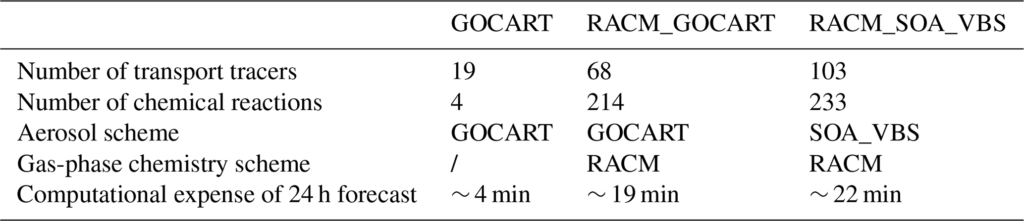
The global Flow-following finite-volume Icosahedral Model (FIM), which was developed in the Global Systems Laboratory (GSL) of NOAA, has been coupled inline with aerosol and gas-phase chemistry schemes of different complexity using the chemistry and aerosol packages from WRF-Chem v3.7, named FIM-Chem v1. The three chemistry schemes include (1) the simple aerosol modules from the Goddard Chemistry Aerosol Radiation and Transport model that includes only simplified sulfur chemistry, black carbon (BC), organic carbon (OC), and sectional dust and sea salt modules (GOCART); (2) the photochemical gas phase of the Regional Atmospheric Chemistry Mechanism (RACM) coupled to GOCART to determine the impact of more realistic gas-phase chemistry on the GOCART aerosol simulations (RACM_GOCART); and (3) a further sophistication within the aerosol modules by replacing GOCART with a modal aerosol scheme that includes secondary organic aerosols (SOAs) based on the volatility basis set (VBS) approach (RACM_SOA_VBS). FIM-Chem is able to simulate aerosol, gas-phase chemical species, and SOA at various spatial resolutions with different levels of complexity and quantify the impact of aerosol on numerical weather prediction (NWP). We compare the results of RACM_GOCART and GOCART schemes which use the default climatological model fields for OH, H2O2, and NO3. We find significant reductions of sulfate that are on the order of 40 % to 80 % over the eastern US and are up to 40 % near the Beijing region over China when using the RACM_GOCART scheme. We also evaluate the model performance by comparing it with the Atmospheric Tomography Mission (ATom-1) aircraft measurements in the summer of 2016. FIM-Chem shows good performance in capturing the aerosol and gas-phase tracers. The model-predicted vertical profiles of biomass burning plumes and dust plumes off western Africa are also reproduced reasonably well.
- Article
(19975 KB) - Full-text XML
- BibTeX
- EndNote


The impacts of aerosol on weather and climate are generally attributed to the direct, semidirect, indirect, and surface albedo effects, with the direct effect predominating radiative forcing over a global scale (e.g., Bauer and Menon, 2012). However, there are significant differences in estimates of direct aerosol radiative forcing between various global aerosol models, particularly with respect to the attribution of forcing to specific aerosol species and sources (Myhre et al., 2013). Discrepancies in direct radiative forcing are also found between global aerosol model results and determinations based on satellite retrievals, with assumptions related to aerosol composition and optical properties as the primary source of difference (e.g., Su et al., 2013). Several processes and steps are necessary to accurately include aerosol effects within a meteorological forecast. Aerosol abundance, composition, and size distribution are the basic quantities needed within calculations of the optical properties, which in turn are used within radiative transfer calculations to calculate heating or cooling rates and are incorporated within the thermodynamic calculations of the numerical forecast.
The importance of aerosol impacts on the meteorological fields for climate modeling has been widely recognized by many studies (e.g., Xie et al., 2013; Yang et al., 2014; H. Wang et al., 2014a; Q. Wang et al., 2014; Colarco et al., 2014). Since it is increasingly common for modeling systems to start using prognostic online aerosol schemes and more accurate emissions, many studies exist that show the importance of including aerosols at least for case studies or over limited time periods. On numerical weather prediction (NWP) timescales (5–10 d), Rodwell and Jung (2008) showed an improvement in forecast skill and general circulation patterns in the tropics and extratropics by using a monthly varying aerosol climatology rather than a fixed climatology in the European Centre for Medium-Range Weather Forecasts (ECMWF) global forecasting system (GFS). The inclusion of the direct and indirect effects of aerosol complexity into a version of the global NWP configuration of the Met Office Unified Model (Met UM) shows that the prognostic aerosol schemes are better able to predict the temporal and spatial variations of atmospheric aerosol optical depth, which is particularly important in cases of large sporadic aerosol events such as large dust storms or forest fires (Mulcahy et al., 2014). The aerosols from biomass burning sources have been shown to have an effect on large-scale weather patterns within global-scale models (e.g., Sakaeda, 2011) and synoptic-scale meteorology within the WRF-Chem regional model (Grell et al., 2011). Toll et al. (2016) showed considerable improvement in forecasts of near-surface conditions during Russian wildfires in summer of 2010 by including the direct radiative effect of realistic aerosol distributions. Likewise, many global models (e.g., Haustein et al., 2012) and regional models (e.g., WRF-Chem, Zhao et al., 2010) have established a clear connection between dust emissions and weather patterns over synoptic to seasonal timescales. While positive impacts of predicted aerosols on weather forecasts have been shown on an episodic basis, a systematic verification of current state-of-the-art operational modeling systems does not yet demonstrate that the impact is statistically significant over longer periods of time to warrant the required additional computational resources (Marécal et al., 2015). Operational forecast systems are usually highly tuned and still use aerosol climatologies. The inclusion of aerosols in the presence of strong sources or sinks should lead to an improvement of predictive skills. A successful example of a short-range weather forecasting coupled with a smoke tracer is the High-Resolution Rapid Refresh coupled with Smoke (HRRR-Smoke) model (Ahmadov et al., 2017). The model forecasts 3-D smoke concentrations and their radiative impacts over the continental US (CONUS) domain at 3 km spatial gridding (https://rapidrefresh.noaa.gov/hrrr/HRRRsmoke/, last access: 13 January 2022).
By applying the chemistry package from WRF-Chem v3.7 into the Flow-following finite-volume Icosahedra Model (FIM, Bleck et al., 2015), named FIM-Chem v1, we essentially make it possible to explore the importance of different levels of complexity in gas and aerosol chemistry, as well as in physics parameterizations on the interaction processes in global modeling systems. FIM is used in the subseasonal experiment (SUBx) for subseasonal to seasonal (S2S) forecasting (Sun et al., 2018a, b) and is now considered a steppingstone towards NOAA's Next Generation Global Prediction System (NGGPS), which will be based on the third-generation non-hydrostatic Finite Volume Cubed Sphere (FV3) dynamic core. The chemistry component created here is designed to be moved flawlessly into FV3. WRF-Chem currently has 63 different gas and aerosol chemistry options, as well as several microphysics and radiation parameterizations, which are coupled to chemistry to simulate direct and indirect aerosol feedback processes. In this study, we demonstrate three examples of different complexities on the aerosol forecasts by FIM-Chem. The current real-time forecast uses simple bulk aerosol modules from the Goddard Chemistry Aerosol Radiation and Transport (GOCART) model, with a simplified chemistry for sulfate production. This chemistry scheme does not include NOx/volatile organic compound (VOC) gas chemistry or secondary organic aerosol (SOA) formation. Currently the real-time GOCART application uses climatological fields of OH, H2O2, and NO3 to drive the oxidation of SO2 and oceanic dimethyl sulfide to sulfate.
Here, we also investigate the sensitivity to the addition of complex gas-phase chemistry and a more reasonable inclusion of secondary organic aerosol formation. Organic matter makes up the significant fraction of the submicron aerosol composition (Zhang et al., 2007), and organic aerosol (OA) along with sulfate and black carbon are believed to be the main anthropogenic contributors to direct radiative forcing on a global scale (Myhre et al., 2013). A computationally efficient SOA parameterization based on the volatility basis set (VBS) approach (Donahue, 2011) was implemented in WRF-Chem by Ahmadov et al. (2012).
To evaluate the model performance, the observation data from the NASA Atmospheric Tomography aircraft mission (ATom-1, 2016) are used, in which the DC-8 is instrumented to make high-frequency in situ measurements of the most the chemical species over the Pacific and Atlantic oceans, and across the Arctic and US, to evaluate the model performance. Section 2 describes some aspects of the FIM and FIM-Chem model, the coupling of aerosol configurations, gas-phase chemical schemes, and an overview of the observation data used to evaluate the model results. The chemical weather forecasts by using three different gas and aerosol chemistry schemes with different levels of complexity are shown in Sect. 3. Section 4 presents the evaluations of the chemical weather forecasts, and the model evaluations are investigated in Sect. 5. We end with a discussion and conclusions in Sect. 6.
2.1 FIM
FIM is a hydrostatic global weather prediction model based on an icosahedral horizontal grid and a hybrid terrain-following/isentropic vertical coordinate (Bleck et al., 2015). Icosahedral grids are generated by projecting an icosahedron onto its enclosing sphere and iteratively subdividing the 20 resulting spherical triangles until a desired spatial resolution is reached. The main attraction of geodesic grids lies in their fairly uniform spatial resolution and in the absence of the two pole singularities found in spherical coordinates. The primary purpose of using a near-isentropic vertical coordinate in a circulation model is to assure that momentum and mass field constituents (potential temperature, moisture, chemical compounds, etc.) are dispersed in the model in a manner emulating reality, namely, along neutrally buoyant surfaces. The FIM model has been tested extensively on real-time medium-range forecasts to prepare it for possible inclusion in operational multi-model ensembles for medium-range to seasonal prediction, and the following simulations are performed at G6 (∼ 128 km) horizontal resolution.
In FIM-Chem, the column physics parameterizations have been taken directly from the 2011 version of the GFS (Bleck et al., 2015). The physical parameterizations include the Grell–Freitas convection parameterization (Grell and Freitas, 2014), the Lin et al. (1983) cloud microphysics scheme, coupled to the model aerosol parameterization and modified to include second-moment effects, and the land surface processes simulated by NCEP's Noah land surface model (Koren et al., 1999; Ek et al., 2003).
2.2 FIM-Chem
FIM-Chem is a version of the FIM model coupled inline with a chemical transport model including three aerosol and gas-phase chemistry schemes of different complexities, where physics and chemistry components of the model are simulated simultaneously. The chemical modules and coupling schemes are adopted from the WRF-Chem model v3.6.1 (Grell et al., 2005; Fast et al., 2006; Powers et al., 2017). The different three chemical schemes have been listed in Table 1 for comparison.
2.2.1 GOCART scheme
The first chemical option is the simplest aerosol modules that from the GOCART model, which includes simplified sulfur chemistry for sulfate simulation from chemical reactions of SO2, H2O2, OH, NO3 and dimethyl sulfide (DMS), bulk aerosols of black carbon (BC), organic carbon (OC), and sectional dust and sea salt. For OC and BC, hydrophobic and hydrophilic components are considered and the chemical reactions using prescribed OH, H2O2, and NO3 fields for gaseous sulfur oxidations (Chin et al., 2000). The dust scheme is using the Air Force Weather Agency (AFWA) scheme with five dust size bins (LeGrand et al., 2019). The bulk vertical dust flux is based on the Marticorena and Bergametti scheme (Marticorena et al., 1995), whereas the particle size distribution is built according to Kok (2011), which is based on the brittle material fragmentation theory. Four size bins are considered for the sea salt simulation. The sea salt emissions from the ocean are highly dependent on the surface wind speed (Chin et al., 2000). In total, there are 19 chemical tracers for transport and four chemical reactions in the GOCART schemes. For a 24 h forecast, it takes about 4 min.
2.2.2 RACM_GOCART scheme
The simple GOCART aerosol scheme does not include photolysis, full gas chemistry, and secondary organic aerosol production, and it normally uses climatological fields of OH, H2O2, and NO3 to drive the oxidation of SO2 and oceanic dimethyl sulfide (DMS) to produce sulfate. Based on the GOCART aerosol module, the second chemical option includes the photochemical gas-phase mechanism of the Regional Atmospheric Chemistry Mechanism (RACM), which is able to determine the impact of the additional gas-phase complexity on the aerosol simulations (RACM_GOCART). The RACM chemistry mechanism is based upon the earlier Regional Acid Deposition Model, version 2 (RADM2) mechanism (Stockwell et al., 1990) and the more detailed Euro-RADM mechanism (Stockwell and Kley, 1994). It includes a full range of photolysis, biogenic VOCs, full NOx/VOC chemistry, and inorganic and organic gaseous species to perform air pollution studies that include rate constants and product yields from the laboratory measurements (Stockwell et al., 1997). The simplified sulfur chemistry for sulfate formation does not use climatological fields of OH, H2O2, and NO3 from the GOCART model to drive the oxidation of SO2 as that in GOCART, and it is replaced by explicitly simulating the gas-phase RACM chemistry. Meanwhile, SO2 is also impacted by the RACM gas-phase chemistry, leading to differences with the GOCART simulations. There are 214 chemical reactions and 68 chemical tracers for transport in the RACM_GOCART scheme. It takes about 19 min for a 24 h forecast.
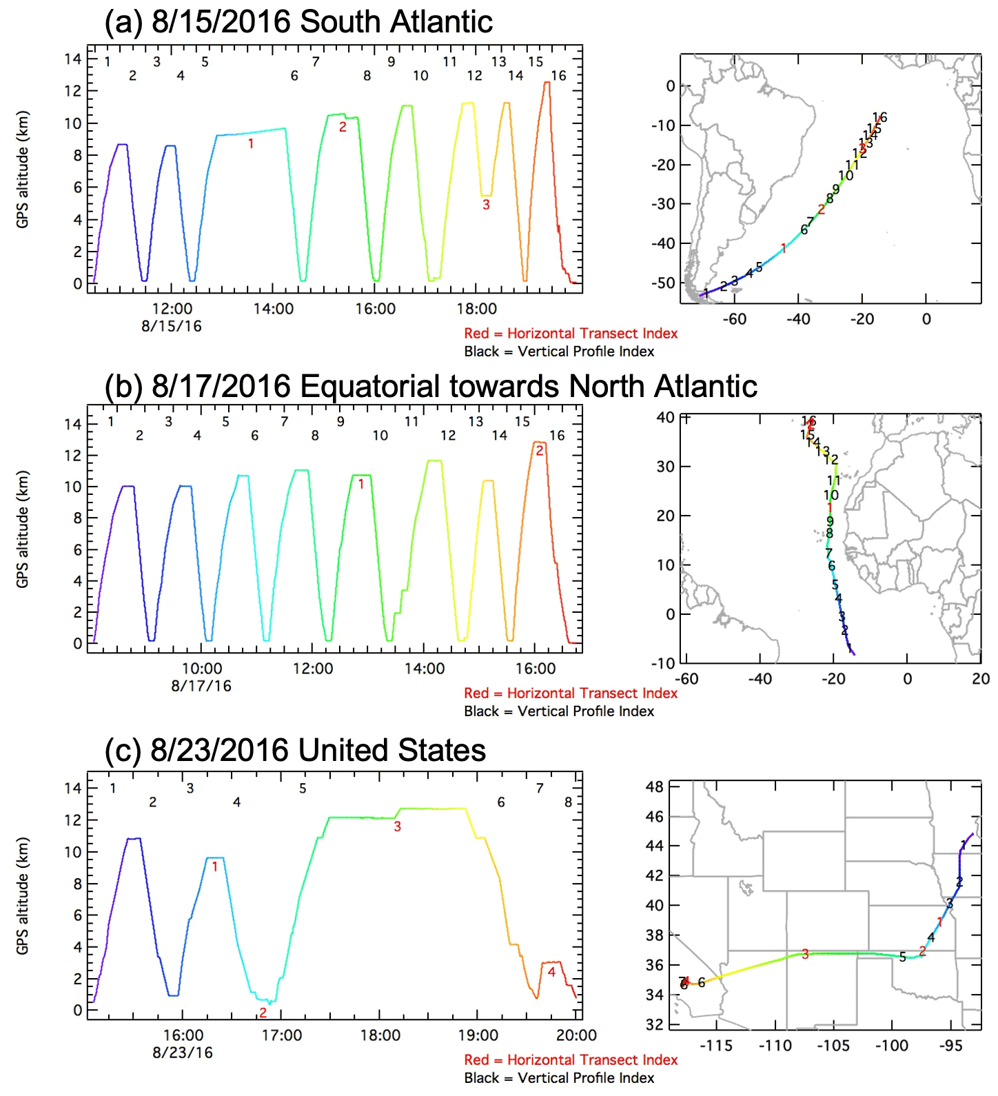
Figure 1Vertical profiles and transect time series of the ATom-1 flight tracks on (a) 15 August over the South Atlantic, Punta Arenas to Ascension, (b) 17 August over the equatorial zone towards the North Atlantic, Ascension to Azores, and 23 August over the United States, Minnesota to southern California in 2016. Dates are indicated in mm/dd/yyyy format.
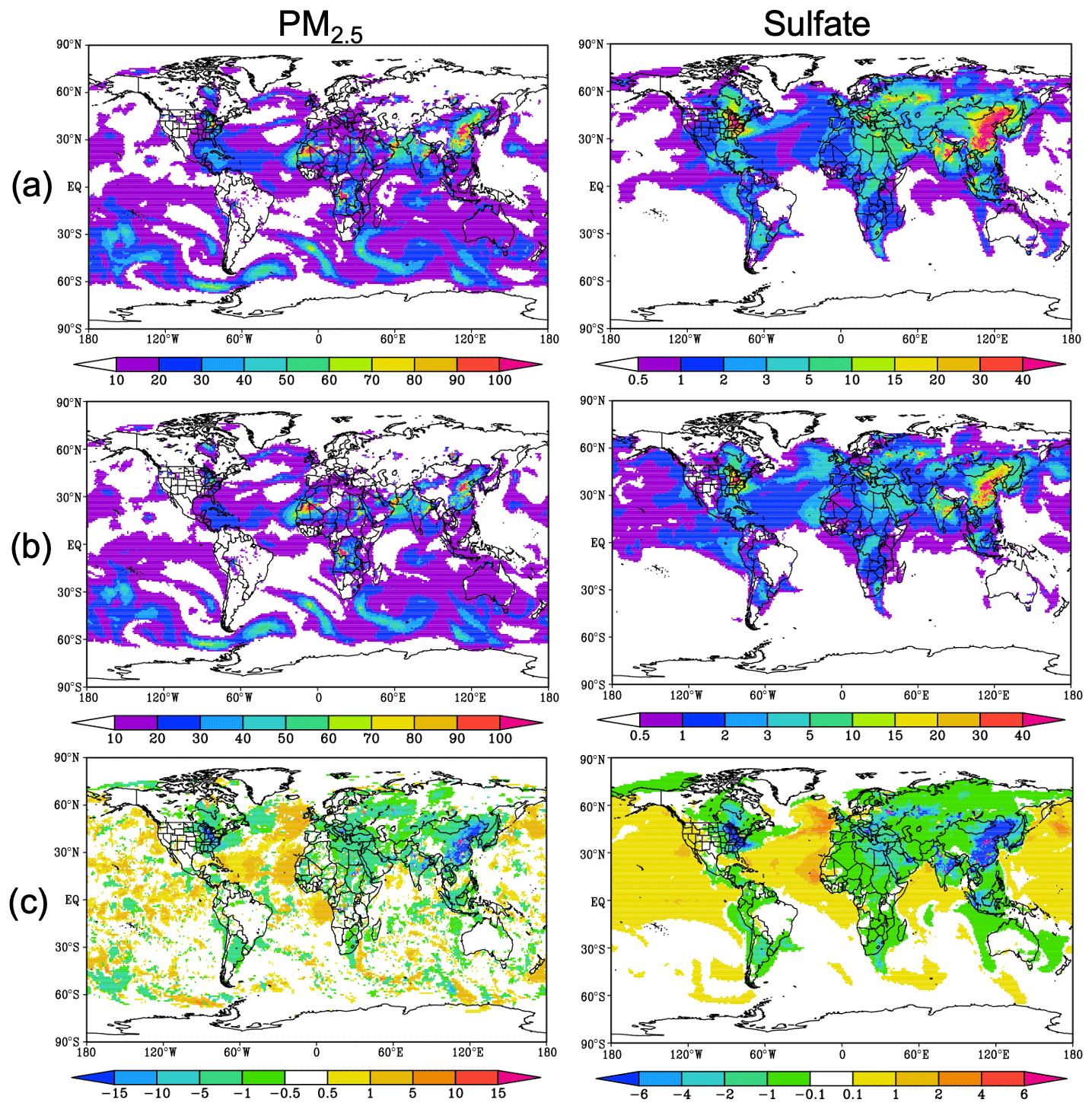
Figure 2The 5 d forecast starting from 00:00 UTC on 29 July 2016 of surface PM2.5 and sulfate using (a) GOCART and (b) RACM_GOCART schemes, and their (c) differences (RACM_GOCART minus GOCART) at 00:00 UTC on 3 August 2016. Unit: µg m−3.
2.2.3 RACM_SOA_VBS scheme
Other than the simple GOCART aerosol scheme in both GOCART and RACM_GOCART, we implemented a more complex gas–aerosol chemistry scheme of RACM_SOA_VBS in FIM-Chem. This scheme includes the RACM-based gas chemistry and the modal aerosol scheme MADE (Modal Aerosol Dynamics Model for Europe) with SOA based on the VBS approach (Ahmadov et al., 2012). The RACM_SOA_VBS scheme includes photolysis reactions for multiple species, full nitrogen and VOC (anthropogenic and biogenic) chemistry, and inorganic and organic aerosols. All the secondary gas species required for SO2 oxidation are simulated explicitly by the gas chemistry scheme here. There are 233 chemical reactions and 103 transported chemical tracers in the RACM_SOA_VBS scheme. It takes about 22 min for a 24 h forecast. The new SOA mechanism contains four volatility bins for each SOA class and their organic vapors that condense onto aerosol. Equilibrium between gas- and particle-phase matter for each bin is assumed in the model. The SOA species are added within the MADE aerosol module, which considers composition within the Aitken and the accumulation modes separately. The VBS approach was included for SOA production, updated SOA yields, and multigenerational VOC oxidation. The VOCs forming SOA are divided into two groups: anthropogenic and biogenic. Isoprene, monoterpenes, and sesquiterpenes are emitted by biogenic sources, while other VOCs are emitted by anthropogenic sources. More detailed descriptions about the VBS approach based on SOA scheme can be found in Ahmadov et al. (2012).
2.2.4 Emission, deposition, and aerosol optical properties
The preprocessor, PREP-CHEM-SRC version 1.5 (Freitas et al., 2011), a comprehensive software tool aiming at preparing emission fields of the chemical species for use in atmospheric-chemistry transport models, is used to generate the emissions for FIM-Chem. It includes the Hemispheric Transport of Air Pollution (HTAP) v2 global anthropogenic emission inventory (Janssens-Maenhout et al., 2015) and biogenic VOC emissions simulated by the Model of Emissions of Gases and Aerosols from Nature (MEGAN) v2.0 parameterization (Guenther et al., 2006). The diurnal variability based on a function of anthropogenic activities is applied to the HTAP emissions, and the diurnal cycle of solar radiation and air temperature is applied to the biogenic emissions. The biomass burning emission estimated by the Brazilian Biomass Burning Emissions Model (3BEM, Longo et al., 2010; Grell et al., 2011) is also included in PREP-CHEM-SRC. The 3BEM is based on near-real-time remote sensing fire products to determine fire emissions and plume rise characteristics (Freitas et al., 2007; Longo et al., 2010). Although the same settings are used for these three schemes in PREP-Chem-SRC, the speciation profiles are modified for each specific mechanism. The fire emissions are updated as they become available and are spatially and temporally distributed according to the fire count locations obtained by remote sensing of the Moderate Resolution Imaging Spectroradiometer (MODIS) aboard the Terra and Aqua satellites (Giglio et al., 2003). The biomass burning emission factors are from Andreae and Merlet (2001). Over the CONUS domain, the MODIS data are replaced by the Wildfire Automated Biomass Algorithm (WF_ABBA) processing system. The WF_ABBA is able to detect and characterize fires in near-real time, providing users with high-temporal-resolution and high-spatial-resolution fire detection data (http://www.ssd.noaa.gov/PS/FIRE/Layers/ABBA/abba.html, last access: 13 January 2022). In the current retrospective forecast of 2016, there is no day lag input for emission in the model. A one-dimensional (1-D) time-dependent cloud model has been implemented to calculate injection heights and emission rates online in all of the three chemical schemes (Freitas et al., 2007).
Similar to the WRF-Chem model, the flux of gases and aerosols from the atmosphere to the surface is calculated by multiplying concentrations of the chemical species in the lowest model layer by the spatially and temporally varying deposition velocities, the inverse of which is proportional to the sum of three characteristic resistances (aerodynamic resistance, sublayer resistance, surface resistance; Grell et al., 2005). The GOCART aerosol dry deposition includes sedimentation (gravitational settling) as a function of particle size and air viscosity, and surface deposition as a function of surface type and meteorological conditions (Wesely, 1989). The dry deposition of sulfate is described differently. In the case of simulations without calculating aerosols explicitly, sulfate is assumed to be presented in the form of aerosol particles, and the dry deposition of aerosol and gas-phase species is parameterized as described in Erisman et al. (1994). For the RACM_SOA_VBS chemical option, the dry deposition velocity of the organic condensable vapors (OCVs) is parameterized as proportional to the model-calculated deposition velocity of a very soluble gas, nitric acid (HNO3). The parameter which determines the fraction (denoted as “depo_fact”) of HNO3 is assumed in the model since no observational constraints are available. The dry deposition velocity of HNO3 is calculated by the model during runtime (Ahmadov et al., 2012). Wet deposition accounts for the scavenging of aerosols in convective updrafts and rainout/washout in large-scale precipitation (Giorgi and Chameides, 1986; Balkanski et al., 1993).
The aerosol optical properties such as extinction, single-scattering albedo, and the asymmetry factor for scattering are computed as a function of wavelength. Each chemical constituent of the aerosol is associated with a complex index of refraction. A detailed description of the computation of aerosol optical properties can be found in Fast et al. (2006) and Barnard et al. (2010).
2.3 Observations
The Atmospheric Tomography Mission (ATom) studies the impact of human-produced air pollution on greenhouse gases and on chemically reactive gases in the atmosphere (Wofsy et al., 2018). ATom deploys instrumentation to sample the atmospheric composition, profiling the atmosphere in the 0.2 to 12 km altitude range. Flights took place in each of the four seasons over a 22-month period. They originated from the Armstrong Flight Research Center in Palmdale, California, flew north to the western Arctic, south to the South Pacific, east to the Atlantic, north to Greenland, and returned to California across central North America over the Pacific and Atlantic oceans from ∼ 80∘ N to ∼ 65∘ S. ATom establishes a single, contiguous global-scale data set. This comprehensive data set is used to improve the representation of chemically reactive gases and short-lived climate forcers in global models of atmospheric chemistry and climate. Comparisons of model forecasts with five flights from the first ATom mission (15–23 August 2016) are shown here as examples of model performance for specific events, such as wildfires and dust storms, or specific conditions such as oceanic versus continental conditions.
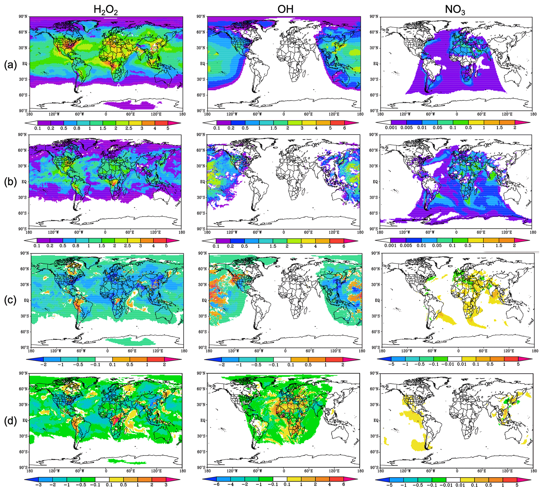
Figure 3Comparisons of 5 d forecast starting from 00:00 UTC on 29 July 2016 of surface H2O2, OH, and NO3 between (a) GOCART and (b) RACM_GOCART schemes, and their differences (RACM_GOCART minus GOCART) at (c) 00:00 UTC and on (d) 3 August 2016. Unit: ppb.
The Particle Analysis by Laser Mass Spectrometry (PALMS) instrument samples the composition of single particles in the atmosphere with diameters within ∼ 150 nm–5 µm range. It measures nearly all components of aerosols from volatiles to refractory elements, including sulfates, nitrates, carbonaceous material, sea salt, and mineral dust (Murphy et al., 2006). The PALMS instrument was originally constructed for high-altitude sampling (Thomson et al., 2000; Murphy et al., 2014) and has since been improved and converted for other research aircraft. Uncertainty in mass concentration products is driven mainly by particle sampling statistics. Relative 1σ statistical errors of 10 %–40 % are typical for each 3 min sample at a mass loading of 0.1 µg m−3 (Froyd et al., 2019). In August 2016, PALMS was sampling on the NASA DC-8 aircraft as part of the ATom program (https://espo.nasa.gov/missions/atom/content/ATom, last access: 13 January 2022). Aerosol composition determinations using the PALMS instrument during ATom have been described and interpreted previously (Murphy et al., 2018, 2019; Schill et al., 2020; Bourgeois et al., 2020). The PALMS mass concentrations for various species are derived by normalizing the fractions of particles of each size and type to size distributions measured by optical particle counters (Froyd et al., 2019).
Figure 1 shows the vertical profiles and transect time series of the ATom-1 flight tracks on 15 and 17 August 2016 over the Atlantic Ocean and on 23 August 2006 over the US. The 15 August flight originates from the southwestern Atlantic and ends near the southern equatorial Atlantic; the 17 August flight is from the southern equatorial Atlantic to the northern Atlantic; and the 23 August flight is from Minnesota to southern California. For analysis and model validations, here we mark 16 vertical tracks and 3 horizontal tracks for 15 August, 16 vertical tracks and 2 horizontal tracks for 17 August, and 8 vertical tracks and 4 horizontal tracks for 23 August.
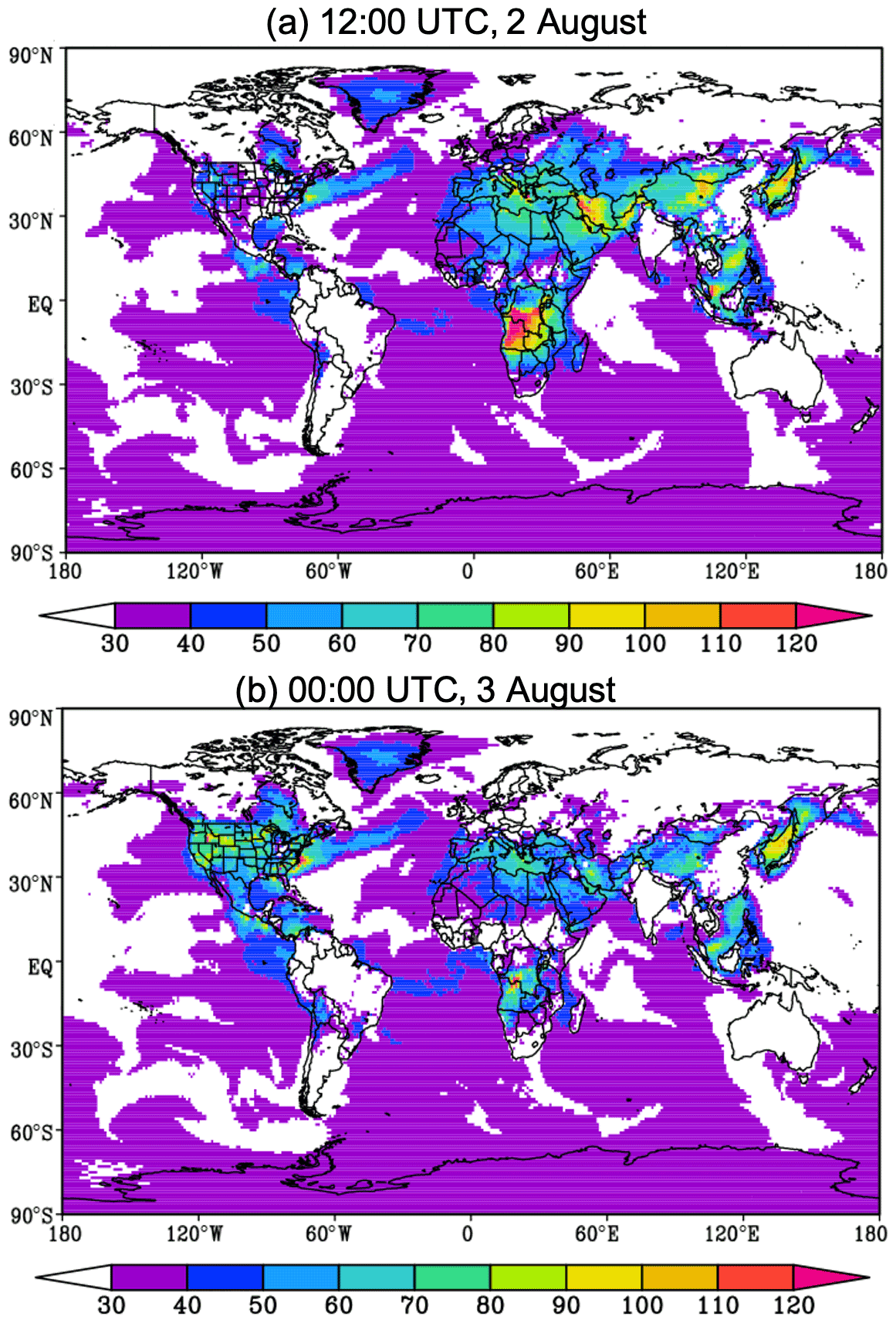
Figure 4The 5 d forecast starting from 00:00 UTC on 29 July 2016 of surface O3 using RACM_GOCART scheme at (a) 12:00 UTC on 2 August and (b) 00:00 UTC on 3 August 2016. Unit: ppb.
We perform a 5 d forecast starting from 00:00 UTC on 29 July 2016, and get the predicted results at 00:00 UTC on 3 August 2016 in Figs. 2 and 3. For the aerosol forecast, the GOCART and RACM_GOCART scheme are quite similar since they are using the same GOCART aerosol module. However, the major difference is the impact of including gas-phase chemistry on aerosol. The simpler GOCART package uses climatological fields for OH, H2O2, and NO3 from previous GEOS model simulations, while these species are explicitly simulated in the RACM_GOCART chemistry mechanism. The PM2.5 concentrations are the sum of BC, OC, sulfate, and the fine bins (diameter < 2.5 µm) of dust and sea salt. The forecast aerosol results of surface PM2.5 and sulfate using GOCART and RACM_GOCART and their differences (RACM_GOCART minus GOCART) are shown in Fig. 2. The general patterns of surface PM2.5 are quite similar in these two schemes, with the maximum surface concentrations of more than 100 µg m−3 over the dust source region of western Africa, part of the southern African fire regions, and part of the polluted areas of south Asia and eastern China. However, the surface concentrations of PM2.5 in GOCART and RACM_GOCART (the latter minus the former) show substantial differences, decreasing more than 15 µg m−3 over the eastern US and 20 µg m−3 over eastern China, when using the RACM_GOCART scheme. The main factor that contributes to the significant differences of surface PM2.5 concentration is sulfate (see right column of Fig. 2). The maximum surface sulfate concentrations are over the eastern US, India, and eastern China. We find the reductions of sulfate are about 10 µg m−3 on the order of 40 %–80 % over the eastern US and are up to 40 % over eastern China in RACM_GOCART (Fig. 2b). The major differences for sulfate production between GOCART and GOCART-RACM are the background fields of H2O2, OH, and NO3. GOCART uses the model climatological backgrounds fields of H2O2, OH, and NO3, while GOCART-RACM uses the online-calculated fields of H2O2, OH, and NO3 from the RACM mechanism.
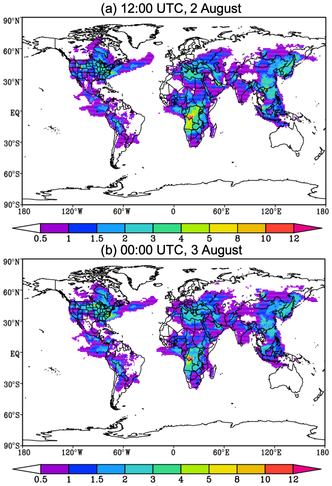
Figure 5The 5 d forecast starting from 00:00 UTC on 29 July 2016 of surface SOA using RACM_SOA_VBS scheme at (a) 12:00 UTC on 2 August and (b) 00:00 UTC on 3 August 2016. Unit: µg m−3.
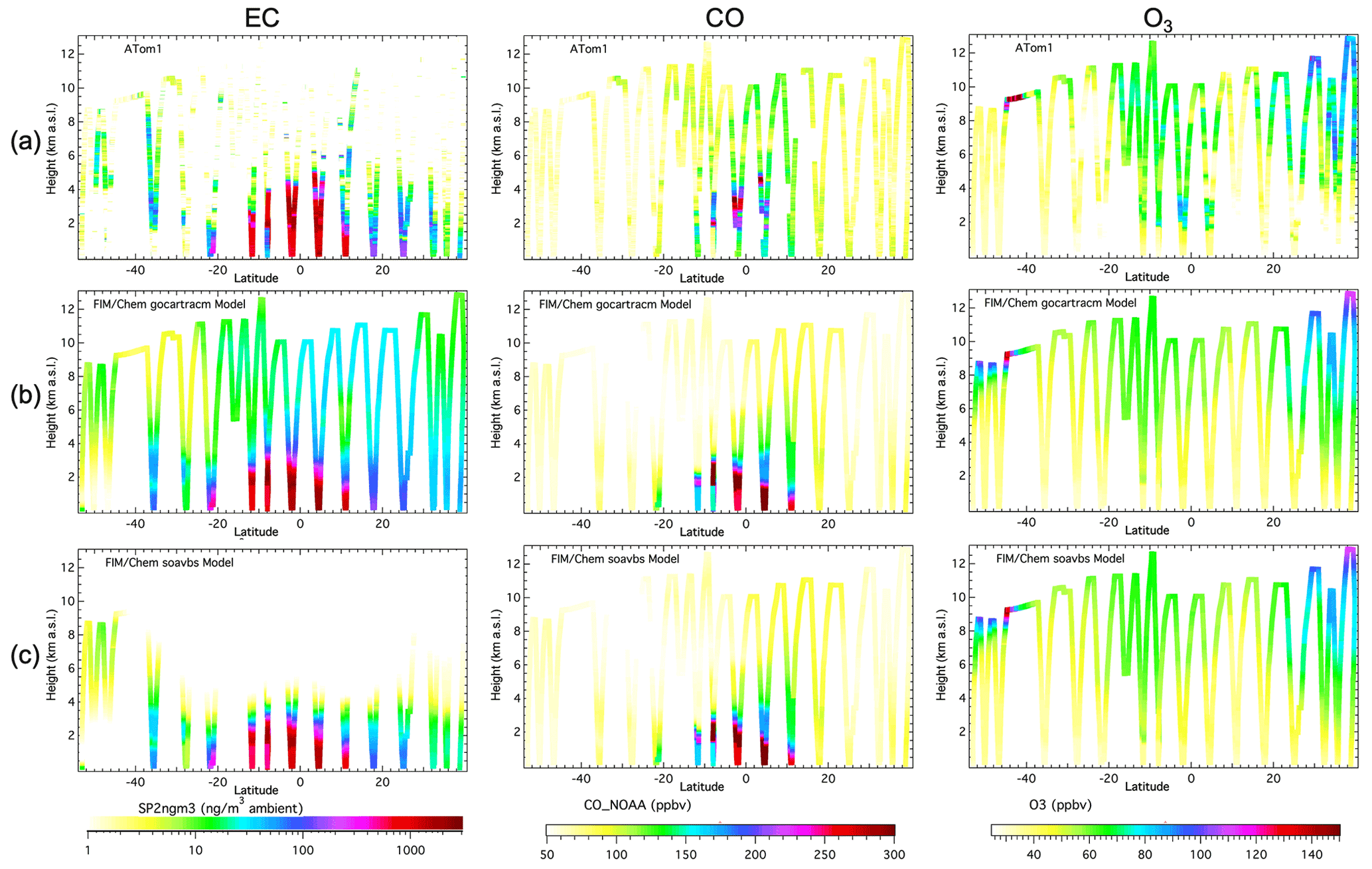
Figure 6Height–latitude profiles of EC (elemental carbon), CO, and O3 over the Atlantic on 15 August and 17 August 2016 for (a) ATom-1; (b) RACM_GOCART; and (c) RACM_SOA_VBS.
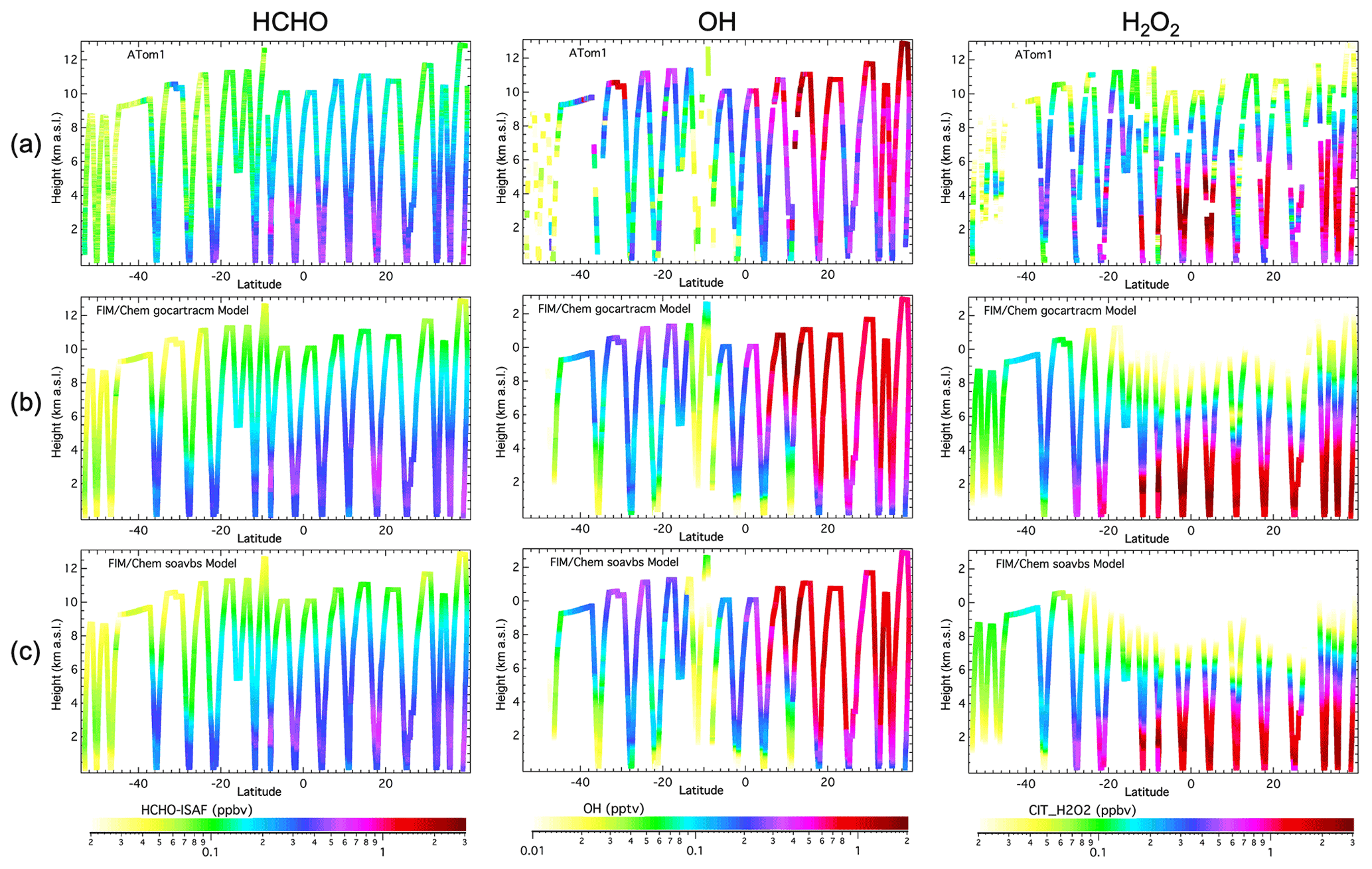
Figure 7Height–latitude profiles of HCHO, OH, and H2O2 over the Atlantic on 15 and 17 August 2016 for (a) ATom-1 observations; (b) RACM_GOCART; and (c) RACM_SOA_VBS.
Figure 3 shows the comparisons of surface H2O2, OH, and NO3 between the GOCART and RACM_GOCART schemes. Globally the prescribed surface H2O2 in GOCART is generally larger than that explicitly simulated by RACM_GOCART. The maximum of surface H2O2 regions over Africa, India, and eastern Asia shows significant diversity. The explicitly real-simulated instantaneous surface H2O2 in RACM_GOCART is much lower, by 40 %–60 %, over India and eastern Asia and 20 % over the eastern US, while it is much higher (>80 %) over central Africa, northeastern regions of Canada, and northwestern areas of South America. Even though the patterns of surface OH are quite comparable in the GOCART and RACM_GOCART schemes at 00:00 UTC, the real-simulated instantaneous surface OH is 80 % lower over eastern China when using the RACM_GOCART scheme. The other big difference is over the western US with the simulated surface OH in RACM_GOCART being much higher over the northwestern US and lower over the southwestern US at 00:00 UTC. The surface NO3 differences are mainly over Africa and the northern Indian Ocean; the real-simulated instantaneous surface NO3 is much larger using the RACM_GOCART scheme at 00:00 UTC. Since surface H2O2 and OH are the major species converting SO2 to sulfate, their decreases cause sulfate reductions over broad areas. The OH differences of the GOCART and RACM_GOCART schemes at 12:00 UTC show a reduction over Africa, India, and Asia, corresponding to the decreasing sulfate over those areas, accounting for the major differences in sulfate production between the two mechanisms.
The RACM_GOCART model is able to predict gas-phase species by using the RACM gas-phase mechanism. Ozone (O3) and other gas pollutants are determined by the emissions of nitrogen oxides and reactive organic species, gas- and aqueous-phase chemical reaction rates, depositions, and meteorological conditions. Figure 4 represents the 5 d surface O3 forecast globally at 12:00 UTC on 2 August and 00:00 UTC on 3 August 2016, which started from 00:00 UTC on 29 July 2016. Similar to other studies, a lot of chemical transport models (CTMs) tend to significantly overestimate surface O3 in the southeast US (Lin et al., 2008; Fiore et al., 2009; Reidmiller et al., 2009; Brown-Steiner et al., 2015; Canty et al., 2015; Travis et al., 2016), which is an important issue for the design of pollution control strategies (McDonald-Buller et al., 2011). We see similar problem in FIM-Chem, where the predicted surface O3 concentration at 00:00 UTC on 3 August 2016 is also overestimated (see Fig. 4b). The relatively low surface O3 is likely due to the O3 titration during the early morning and nighttime periods. It well known that the O3 production involves complex chemistry driven by emissions of anthropogenic nitrogen oxide radicals (NOx = NO + NO2) and isoprene from biogenic emissions. The primary basis of O3 may be due to the inventory of HTAP v2 anthropogenic emission over North America, which is from the US EPA's 2005 National Emission Inventory (2005 NEI). A few studies have pointed out that the NOx emissions in the 2005 and 2011 NEI inventories from the EPA are too high (Brioude, 2011; Travis et al., 2016) over the US. They must be reduced by 30 %–60 % from mobile and industrial sources in the 2011 NEI (Travis et al., 2016), while the NOx emissions over the United States should be reduced more for the 2016 simulation since the 2005 NEI NOx emissions are much larger than those of the 2011 NEI (https://cfpub.epa.gov/roe/, last access: 13 January 2022). Also, the dry depositions of ozone and isoprene emissions, and the loss of NOx from formation of isoprene nitrates could also result in these overestimations (Lin et al., 2008; Fiore et al., 2005).
The SOA parameterization based on the volatility basis and VBS approach applied within FIM-Chem has the ability to simulate and predict SOA using the RACM_SOA_VBS scheme (Ahmadov et al., 2012), which includes the anthropogenic secondary organic aerosols (ASOAs) and biogenic secondary organic aerosols (BSOAs) for both the nucleation and accumulation modes. Figure 5 shows the predicted SOA at 12:00 UTC on 2 August and 00:00 UTC on 3 August 2016. The maximum surface SOA concentrations are over southern Africa, which may be caused by the wildfire emissions. The eastern US, western Europe, and eastern Asia are the other high SOA concentration areas. There is no significant diurnal variability for the SOA spatial distributions, and the diurnal cycle of fire emission has not been included.
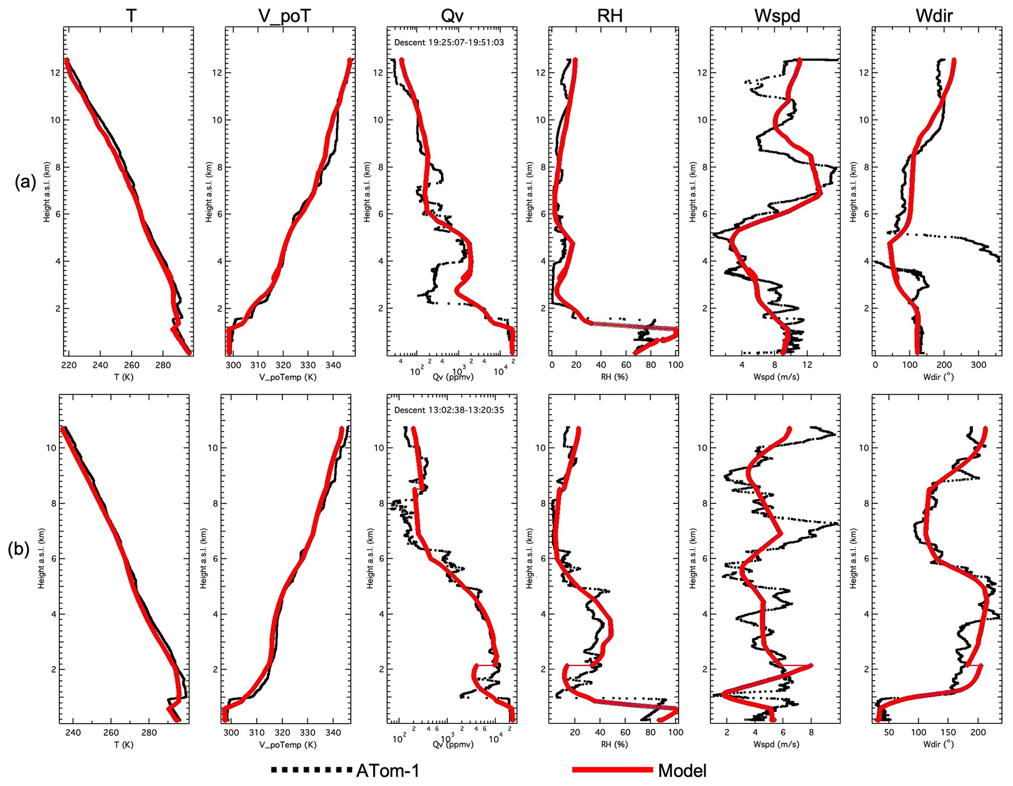
Figure 8ATom-1 observations and model results for temperature, virtual potential temperature, water vapor, relative humidity, wind speed, and wind direction in the (a) biomass burning and (b) dust events. The biomass burning plume is from 15 August 2016, profile no. 16 near 20∘ S, while the Saharan dust plume is from 17 August 2016, profile no. 10 near 25∘ N.

Figure 9Comparisons between ATom-1 observations and model vertical profiles of EC, sea salt, dust, O3, and CO in the (a) biomass burning and (b) dust storm events. The biomass burning plume is from 15 August 2016, profile no. 16 near 20∘ S, while the Saharan dust plume is from 17 August 2016, profile no. 10 near 25∘ N. Green and blue lines are nearly identical for aerosol.
The retrospective daily forecast uses cycling for the chemical fields since no data assimilation is included in the chemical model. Meteorological fields are initialized by the GFS meteorological fields every 24 h, while the chemical fields from the last output (forecast at 24:00 UTC or 00:00 UTC of the next day) are used as the initial conditions of the current forecast (00:00 UTC). Stratospheric O3 above the tropopause is taken from satellite-derived fields available within GFS. For the ATom-1 forecast periods, considering there is no initial chemical conditions, we performed a 2-week spin-up period (from 15 to 28 July) before the first observational comparison day (29 July 2016) to help get a more realistic initial chemical conditions for the ATom-1 forecast period. It should be noted that stratospheric chemistry is incomplete (no halogen chemistry) in the model.
In this section, we compare 24 h forecasts of FIM-Chem for the major aerosols and gas tracers for the three different chemical schemes listed above. The FIM-Chem model results are sampled at the grid with nearest latitude and longitude, then interpolated logarithmically in altitude according to the ATom-1 measurements. Temporally, 1 s measurements are matched to the nearest hour of the FIM-Chem hourly model output, which translates into a spatial uncertainty of ∼ 128 km, or approximately one model grid cell, for typical DC-8 airspeeds.

Figure 10Height–latitude profiles of EC and sulfate over the United States on 23 August 2016 for (a) ATom-1; (b) GOCART; (c) RACM_GOCART; and (d) RACM_SOA_VBS.
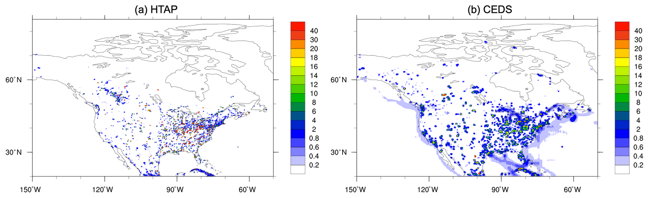
Figure 11Anthropogenic emissions of SO2 of (a) HTAP and (b) Community Emissions Data System (CEDS) inventories for August. Unit: .
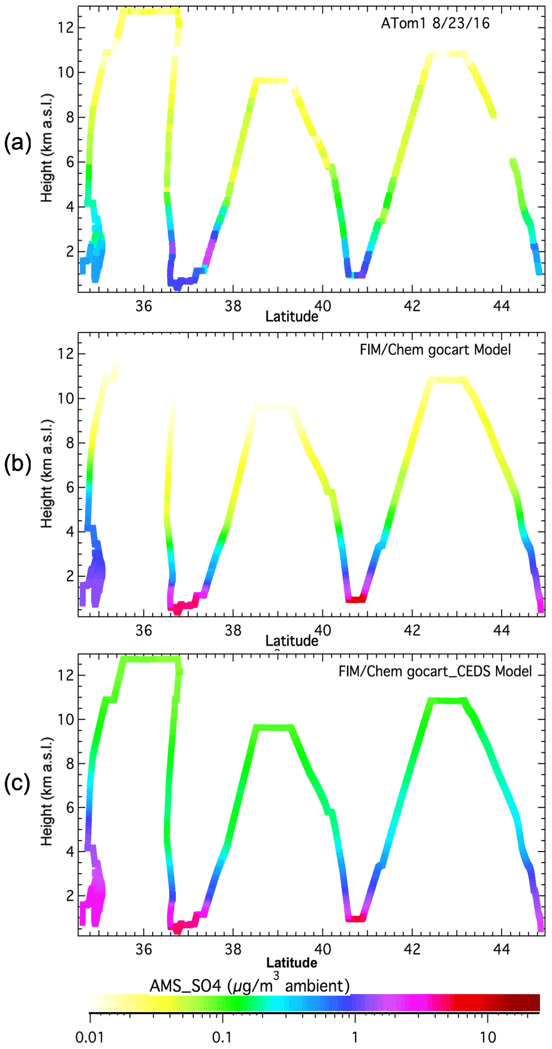
Figure 12Height–latitude profiles of sulfate over the United States on 23 August 2016 for (a) ATom-1, (b) GOCART with HTAP, and (c) GOCART with CEDS anthropogenic emission.
4.1 Comparisons of the gas and aerosol species between FIM-Chem and the ATom-1 measurements over the Atlantic
The comparisons between RACM_GOCART and RACM_SOA_VBS schemes for the chemical species, e.g., EC (elemental carbon, which is the same as BC), CO, and O3, that are mainly affected by the biomass burning emissions from wildfires during 15 and 17 August, are shown in Fig. 6. The model shows very good performance in reproducing the profiles of EC and CO, especially capturing the biomass burning plumes near the tropics. But it also shows some differences for EC in the results of the GOCART (figures not shown here since they are almost the same as those of RACM_GOCART) and RACM_GOCART schemes above 4–5 km, where model results are overestimated. Generally, the EC performance of RACM_GOCART is much better at low altitudes but has a high bias at high altitudes where the RACM_SOA_VBS performs well. After investigating, we noticed that the GOCART and RACM_GOCART aerosol modules both assume there is no wet deposition for externally mixed, hydrophobic BC, only for hydrophilic BC. This assumption would result in the overestimation of EC at higher levels due to less washout of hydrophobic BC. Other models with simple wet removal schemes have shown similar overestimation of EC in the upper troposphere (Schwarz et al., 2013; Yu et al., 2019). However, aerosols in the RACM_SOA_VBS scheme are internally mixed, so there is a much larger wet deposition and less EC in the upper levels. This an important difference about the carbonaceous aerosol for both hydrophobic BC and OC in the wet removal. The comparison with the observations provides a good resource for further improvements within the wet removal parameterization. The second column in Fig. 6 compares CO for the observations, RACM_GOCART, and RACM_SOA_VBS schemes. Overall, the forecast is able to capture the observed latitude–height profiles of the CO mixing ratio. However, they both show high biases at low altitude (about ∼ 2 km) in the tropics. Other than that, there are still some differences such as the underestimated CO mixing ratio above 6 km over the tropics and overestimates near the surface. Also, the model does not reproduce the fire plume height correctly for the biomass burning emissions over this area, which may be due to vertical transport or lower injection heights near the fire source region. For O3, the model is able to consistently capture O3 mixing ratios with both RACM_GOCART and RACM_SOA_VBS schemes, including the stratospheric intrusion near 40∘ S at about 9 km height, though it is slightly higher near 40∘ N at about 12 km height. We find that over equatorial areas at about 2–4 km height, the modeled O3 mixing ratio is underestimated by about 30 %. This may also relate to the injection height of biomass burning that resulted in much lower CO at this altitude, since CO is an important precursor for O3 production. Near the surface, the overpredicted CO in the RACM_GOCART and RACM_SOA_VBS schemes does not result in high O3. It may be related to O3 precursors other than CO, such as missing VOC and NOx sources. Large uncertainties in both the biogenic and anthropogenic emission inventories are expected over western Africa. Besides the aerosol and gas tracers associated with the biomass burning emissions, we also compare HCHO, OH, and H2O2, which are important precursors or oxidants to many other species within the RACM_GOCART and RACM_SOA_VBS schemes (see Fig. 7). Generally, the pattern of the modeled HCHO mixing ratio is almost the same as that of the ATom-1 measurements. The variations from south to north are captured by these two schemes, with the exception of a little underestimation near about 10 km height. For OH, the model reproduces the vertical and temporal variations, including the large mixing ratios over the Northern Hemisphere. Some slight differences are apparent, e.g., overestimations over 44∘ S at 3–9 km height and underestimations over 40∘ N above 10 km height. Similarly, there is more spatial variability in the ATom-1 measurement of H2O2. Above 6 km, the model overestimates H2O2 south of 40∘ S and overestimates it from 20∘ S to the Northern Hemisphere above 6 km. Overall, the model and ATom-1 measurement are more consistent at lower altitudes for H2O2.
Figures 8 and 9 show more detailed comparisons for vertical tracks of meteorological fields and chemical species in the biomass burning (Fig. 9a) and dust events (Fig. 9b). For the biomass burning plume, the 16th vertical profile on 15 August 2016 near 20∘ S is shown, while the 10th profile on 17 August 2016 near 25∘ N for the Saharan dust plume is shown. The comparison of the meteorological fields of temperature, virtual potential temperature, water vapor, relative humidity, wind speed, and wind direction is shown in Fig. 8 and does not change between the different chemical options. The model-forecasted temperature and virtual potential temperature almost overlap the ATom-1 measurements for both the 15 and 17 August vertical tracks. For water vapor and relative humidity, the variations of the vertical profiles are also reproduced by the model, except there are some smaller peaks in the observed profiles. There are still some differences between model and ATom-1 observations for wind speed and wind direction, which may be due to model vertical resolution. Overall, the model is able to capture the general vertical variations. For the chemical species (see Fig. 9), the modeled EC using the GOCART scheme is almost identical to that by the RACM_GOCART scheme (the green line is overlapped by the blue line). Both EC concentration plots show a vertical variation of decreasing with altitude and the concentrations are overestimated above 2 km in the biomass burning plume (see Fig. 9a) and above 4 km in dust storm (see Fig. 9b). The results using the RACM_SOA_VBS scheme show much better performance in capturing the vertical variations of EC. Other than a slight overestimation at 2–4 km biomass plume (see Fig. 9a, first column), the EC vertical profile is very consistent to that of the observation when using the RACM_SOA_VBS scheme. In the biomass burning event (see Fig. 9b first column), the modeled vertical profile with the RACM_SOA_VBS scheme captures the general changes of the vertical variations much better than those of the GOCART and RACM_GOCART schemes. As mentioned, previously, the assumption of no wet deposition for hydrophobic BC is the main reason leading to less EC at high altitude in the RACM_SOA_VBS scheme compared to the GOCART and RACM_GOCART schemes. Due to less available observed data for sea salt, it is difficult to perform specific comparisons, but both the observation and model show strong decreases with altitude. During the dust event (see Fig. 9b, third column), even though the modeled dust concentrations are lower at about 2–6 km than the observed concentrations, they are close to the observations at the surface and upper levels. For the gas-phase species, the model results are from GOCART_RACM (blue line) and RACM_SOA_VBS (red line) schemes. The observed O3 in the biomass burning event (see Fig. 9a, fourth column) shows a peak at about 2 km height, then it decreases with altitude, but increases again at about 5–9 km height. The model results from these two schemes are quite consistent. They both indicate a slight enhancement at 1.5 km height, though it is not able to capture the magnitude of the observed peak, which is underestimated by ∼ 50 %. For CO, the model can reproduce the peak at about 2 km height very well, though it overestimates the mixing ratio by 25 % below 1 km in the biomass burning event (see Fig. 9a, fifth column). The detailed variations of the O3 and CO vertical profiles still show some slight differences between the model and observation, but the model generally forecasts the vertical changes with altitude, and the CO using RACM_GOCART is slightly lower than that of the RACM_SOA_VBS scheme above 5 km height.

Figure 13Height–latitude profiles of OH and H2O2 over the United States on 23 August 2016 for (a) ATom-1; (b) GOCART; (c) RACM_GOCART; and (d) RACM_SOA_VBS.
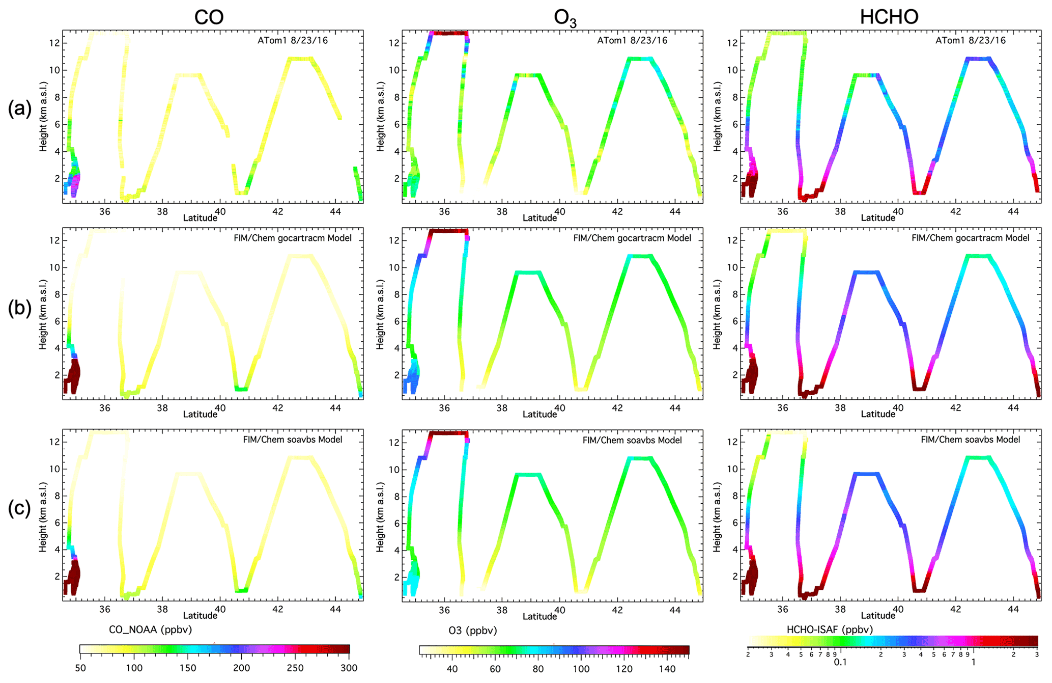
Figure 14Height–latitude profiles of CO, O3, and HCHO over the United States on 23 August 2016 for (a) ATom-1; (b) RACM_GOCART; and (c) RACM_SOA_VBS.
4.2 Comparisons of aerosols and gas tracers between FIM-Chem and ATom-1 over the United States
Figure 10 shows the comparisons of EC and sulfate between ATOM-1 measurements and FIM-Chem model with three different chemical schemes over the United States. Other than the underestimates of wet removal for EC in GOCART and RACM_GOCART schemes that result in the overpredicted EC concentrations above 4 km height, the near-surface (below 4 km) EC concentrations over southern California are also higher than the observation. The overestimate over southern California is also shown in the RACM_SOA_VBS scheme. Similarly, the predicted sulfate concentrations over southern California are much higher than the observation too. Also, the surface sulfate concentrations throughout the US are much higher than those of observations. In the FIM-Chem model, the anthropogenic emissions are from the HTAP v2.1 inventory, which is based on the 2005 NEI over the United States. However, the BC emissions have declined by 50 % in California from 1980 to 2008 following a parallel trend the reduction of fossil fuel BC emissions (Bahadur et al., 2011). The older emission inventory with relatively higher anthropogenic emissions of BC and SO2 may possibly induce the overestimates of near-surface BC and sulfate concentrations for the 2016 simulation in the model results over southern California and other areas. To test this hypothesis, we performed the same GOCART retrospective experiment using the Community Emissions Data System (CEDS) anthropogenic emission (Hoesly et al., 2018) instead of the HTAP v2.1 inventory. The CEDS anthropogenic emission is much stronger than HTAP over California for SO2 (see Fig. 11). Thus, a significant enhancement in sulfate concentration near the surface of California is seen when using CEDS emissions, as shown in Fig. 12. For the sulfate concentrations at upper levels, the GOCART scheme (see Fig. 10b, second column) using the background fields of H2O2, OH, and NO3 shows much better performance in capturing the relatively lower sulfate at upper levels compared to the other two schemes.
Figure 13 shows the comparisons of OH and H2O2 in GOCART, RACM_GOCART, and RACM_SOA_VBS with ATom-1 observations. It can be seen that the prescribed OH is close to the ATom-1 observation, which may be the major factor contributing to better sulfate agreement in GOCART. Considering that the sulfur chemical reaction mechanism and the aerosol scheme in RACM_SOA_VBS are completely different from those in GOCART and RACM_GOCART, the comparison of oxidants may not be the only reason causing the differences, which needs further analysis. For the gas species, we compare CO, HCHO, and O3 (see Fig. 14) using the RACM_GOCART and RACM_SOA_VBS schemes with the observation. Generally, the model cases using either RACM_GOCART or RACM_SOA_VBS scheme show good performance in capturing the CO and HCHO mixing ratios both at the surface and in the free troposphere. But they are both higher than the observations near the surface over southern California, similar to EC and sulfate concentrations. This may be also associated with the overestimation of anthropogenic emissions in the 2005 NEI over the United States for the year 2016. Since CO and HCHO are precursors for O3 production, the simulated O3 also shows slight enhancements compared to the observations that may be due to the higher CO and HCHO. Other than that, the model is able to reproduce the O3 profile over the US reasonably well, including the O3 stratospheric intrusions at the upper levels. The simulated H2O2 in both RACM_GOCART and RACM_SOA_VBS schemes shows better agreement with the observations at the upper levels than the prescribed H2O2 fields in GOCART (Fig. 13), while the much lower H2O2 near the surface in the RACM_SOA_VBS may be associated with better O3 performance near the surface (Fig. 13).
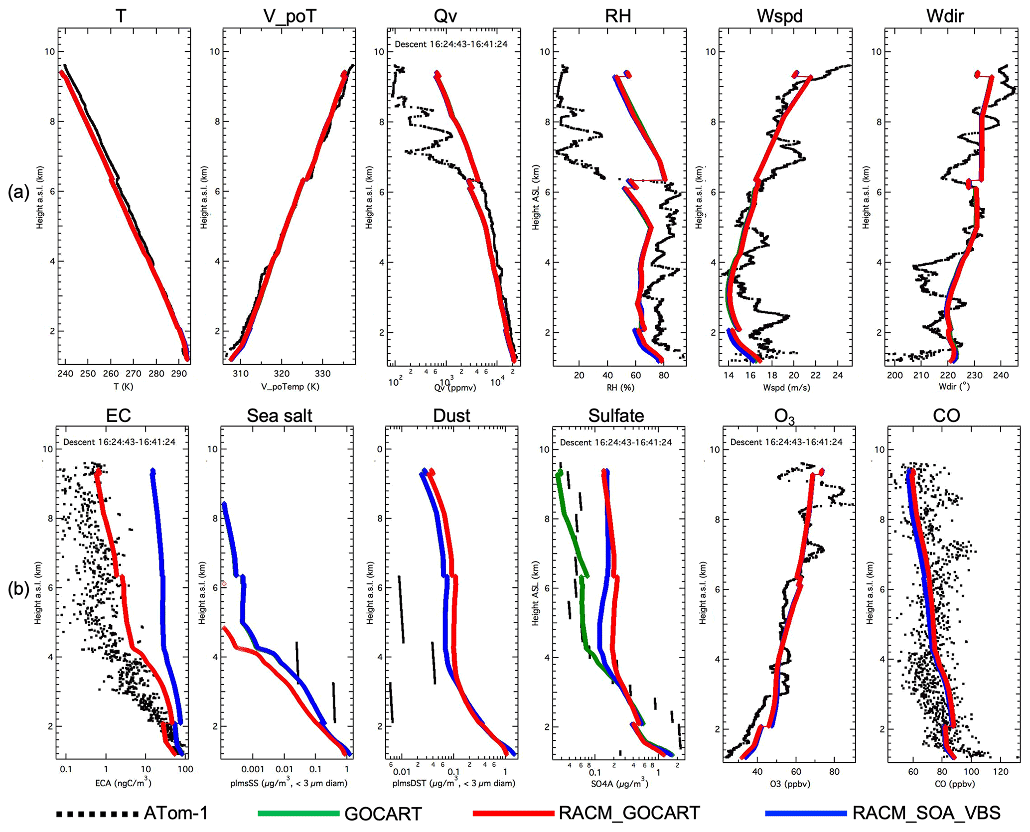
Figure 15Observations and model results for profile no. 4 on 23 August 2016 over southeastern Kansas.
Figure 15 focuses on the fourth vertical profile over Kansas on 23 August 2016. The model results with different chemical schemes are very consistent in simulating the meteorological fields. The modeled temperature and virtual potential temperature show nearly exact agreement with the observations. But there are still some shortcomings in forecast water vapor and relative humidity, especially above 6 km, where the model results are overpredicted by nearly a factor of 2 and with less vertical variability. The vertical trends of modeled wind speed and wind direction are close to the observed changes that increase with altitude. Similar to Fig. 9, the EC vertical profile using the RACM_SOA_VBS scheme, without the hydrophobic assumption in wet removal, is similar to that of the observations while the other two schemes significantly overpredict it. Both the observations and models show a decreasing vertical trend for sea salt and dust. The GOCART scheme is able to reproduce the sulfate, except for the underestimate at 1.5–3 km. Otherwise, it almost overlaps the observed profile at the upper levels. The O3 vertical profile is reproduced by the model using both RACM_GOCART and RACM_SOA_VBS schemes except a slight peak near 9 km, where the model is not able to capture the enhanced variability. The CO measurements have more fluctuations, but the model roughly shows the major features of the vertical changes with altitude.
For the aerosol size range of the GOCART scheme, the PALMS data set allows for model evaluation of the default sea salt emission algorithms by summing those bins less than 3 µm in the model results. The comparisons between the GOCART forecasts and ATom-1 data for all sea salt observations below 6 km are shown in Fig. 16. Different colors show different flight dates from 15 (blue dots), 17 (green dots), 20 (orange), 22 (red), and 23 August (purple). Generally, modeled sea salt appears too high, especially on flights on 15 (blue dots), 20 (orange dots), and 23 August (purple dots) above ∼ 4 km. Some high values below ∼ 4 km are reproduced by the models on the flight of 17 August (green dots). Some of the disagreement may be due to uncertainties in the size range of sea salt observations, particularly the upper cutoff of 3 µm that is approximate (Murphy et al., 2019).

We also investigate the relationships of some key species for the biomass burning plumes observed on 15 and 17 August 2016 between 22∘ S and 22∘ N below 6 km (Fig. 17) for the RACM_SOA_VBS scheme. The color bar indicates the latitude from south to north. Relative to CO, the model biomass burning emission ratios are reasonable for EC, with the modeled ratio (black color dots) somewhat lower than the observations (color dots). We note that in Fig. 6, O3 in the biomass burning region for the RACM_SOA_VBS scheme is underpredicted. To analyze this O3 bias in more detail, scatter plots of modeled and observed NOy versus CO and O3 versus NOy between 22∘ S and 12∘ N below 6 km altitude are shown in Fig. 17b and d, respectively. The observations in Fig. 17d show a much different and better-defined slope of O3 versus NOy compared to the model using the RACM_SOA_VBS scheme. NOy, which is emitted entirely as NOx in fresh plumes, is much higher in the model, suppressing OH (e.g., Fig. 7), HO2, and subsequent ozone formation. The NOy-to-CO ratios in Fig. 17b show evidence in the model of NOy removal through HNO3 scavenging, but it is clear the NOy- (or NOx)-to-CO emission ratio is too high in the fire emissions. The CO emissions themselves appear too high (as also shown in Fig. 6). Other factors, such as VOC emission ratios or photolysis effects from convective clouds, may come into play, but these emission overestimates appear to put the biomass burning region in a different photochemical regime than that shown in the ATom-1 observations.
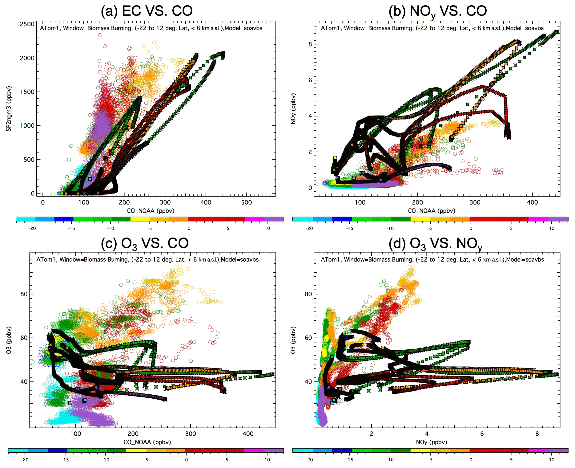
Figure 17Model (black dot) and observation (color dot) ratios of (a) EC relative to CO; (b) NOy relative to CO; (c) O3 relative to CO; and (d) O3 relative to NOy. Color scale indicates degrees latitude.
A two-way fully inline coupled global weather–chemistry prediction model (FIM-Chem) has been developed at NOAA Global Systems Laboratory (GSL) to forecast the chemical composition and quantify the impacts on NWP. Three different gas–aerosol chemistry schemes – GOCART, RACM_GOCART, and RACM_SOA_VBS from WRF-Chem – have been implemented into FIM-Chem with some modifications for different options of chemical schemes. The major conclusions are summarized as follows:
First, the RACM_GOCART mechanism with explicitly simulated H2O2, OH, and NO3 is compared to the base GOCART mechanism, having a simple parameterization of sulfur chemistry using prescribed background fields of OH, H2O2, and NO3. The explicit treatment results in about 10 µg m−3 reductions of sulfate and 15 µg m−3 of PM2.5 over the eastern US, as well as more than 20 µg reductions of PM2.5 over eastern China. Meanwhile, the simulated instantaneous H2O2 is lower by 20 % over the eastern US and 40 %–60 % over India and eastern Asia, while the OH is 80 % lower over eastern China in the RACM_GOCART scheme.
In this study, the evaluation and analysis of model performance are focused on the fire events over the eastern Atlantic from south to north on 15 and 17 August 2016, and the flight over the United States from Minnesota to southern California using the NASA ATom-1 observations.
For the evaluation over the Atlantic, the GOCART and RACM_GOCART results are very consistent in forecasting sulfate, sea salt, and EC due to the same aerosol mechanism. For the fire events sampled near the equatorial Atlantic (e.g., Fig. 6), the GOCART and RACM_GOCART schemes show good performance in reproducing the profiles of EC, and CO is captured reasonably well with the RACM_GOCART and RACM_SOA_VBS schemes. Generally, EC is simulated well by GOCART and RACM_GOCART mechanisms up to 4 km, but above this the mechanisms are biased high, while EC in the RACM_SOA_VBS scheme shows much better performance than that of the GOCART and RACM_GOCART schemes at the upper levels. This is because it is assumed there is no wet deposition for hydrophobic BC in the GOCART and RACM_GOCART schemes, which results in an underestimate of EC wet removal and overestimate of EC concentrations at higher levels. The CO mixing ratio above ∼ 2 km is underestimated over the tropics and overestimated at altitudes below ∼ 2 km, which may be related to lower simulated fire injection heights in the model. Otherwise, the general CO profiles are well reproduced. Both the RACM_GOCART and RACM_SOA_VBS schemes are able to consistently reproduce O3 mixing ratios, including the stratospheric intrusion above ∼ 9 km at 40∘ S. There is some slight underestimation of O3 near the tropics, which might be associated with the underprediction of CO outside the biomass burning signature region. We also evaluated other gas-phase species: HCHO, OH, and H2O2, which are important precursors to many other chemical species within the RACM_GOCART and RACM_SOA_VBS schemes (see Fig. 7). Generally, the patterns of the modeled HCHO, OH, and H2O2 mixing ratio are almost the same as those of the ATom-1 observations except for some underestimates above 9 km for HCHO and OH at some latitudes, and some overestimates of H2O2 above 6 km in the Southern Hemisphere.
For the evaluation from Minnesota to southern California, all of the chemical schemes are able to reproduce the general vertical gradients seen in the observations. The RACM_SOA_VBS scheme is able to reproduce the vertical profile of EC much better than that of the GOCART and RACM_GOCART schemes, which overestimate the EC concentrations above 2–4 km due to the assumption of no wet deposition for hydrophobic BC. This comparison highlights the value of the ATom-1 data in examining basic assumptions within the wet removal parametrization of carbonaceous aerosol in the GOCART mechanism. The high SO2 emissions from either anthropogenic or fire sources play an important role in enhancing the sulfate production. There are high biases above ∼ 3 km for sulfate in the RACM_GOCART and RACM_SOA_VBS schemes. Results from the RACM_GOCART and RACM_SOA_VBS schemes show consistency with observed O3 and CO vertical profiles during the fire events. Both schemes show a slight enhancement of O3 at 1.5 km even though it underestimates the magnitude of the observed peak. For CO, the model results capture the peak at about 2 km very well but overestimates the mixing ratio by about 30 % near the surface. For the gas-phase species, the model either using the RACM_GOCART or RACM_SOA_VBS scheme shows very good ability in forecasting the CO, O3, and HCHO mixing ratio both at the surface and free troposphere, including the O3 stratospheric intrusions at the upper levels (Fig. 14). For CO, a precursor for O3 production, there appears to be overestimated emissions over California causing much higher surface mixing ratios in the forecasts than observed. For the comparisons of vertical profiles over California on 23 August 2016, the modeled meteorological fields of temperature and potential temperature show agreement with the observations. The modeled water vapor and relative humidity are consistent with observations below 6 km though they are overestimated above 6 km. The RACM_SOA_VBS scheme shows the best agreement with EC. For sulfate, the GOCART scheme is almost the same as the observation above 3 km, while it overestimates near the surface due to the high anthropogenic emissions used within the inventory. The simulated O3 and CO vertical profiles almost overlap with the ATom-1 measurements but with less vertical variability. Though data are somewhat sparse in our analysis, the sea salt emission algorithm appears to be a model component that could be improved due to apparent consistent overestimation.
The scatter plots of sea salt and gas tracers from biomass burning plumes shows that modeled sea salt appear too high, and some of the disagreement may be due to uncertainties in the size range of sea salt observations (Fig. 16), and the NOy- (or NOx)-to-CO emission ratio is too high in the fire emissions (Fig. 17). These emission overestimates may put the biomass burning region in a different photochemical regime than that shown in the ATom-1 observations.
The comparison in this study successfully demonstrates that the FIM-Chem model with three difference chemical schemes show good performance in forecasting the chemical composition for both aerosol and gas-phase tracers when compared with the high-temporal-resolution (1 s) observations of ATom-1. The wet removal assumption for hydrophobic BC is not reasonable, which needs to be improved in the GOCART and RACM_GOCART schemes. It is not necessary to use the complexity of a gas-phase scheme if the focus is only on aerosol forecasts, in order to save time and computer resources. Using anthropogenic emissions for the specific year of the simulation may help to improve the forecasts. Also, a new dynamic core of FV3 developed by the Geophysical Fluid Dynamics Laboratory (GFDL) will be used to replace FIM and coupled with the chemical schemes in the NGGPS, as FV3GFS-Chem, by using that to demonstrate the chemical impacts on NWP.
Basically, the chemical modules of GOCART, RACM_GOCART, and RACM_SOA_VBS are based on the WRF-Chem 3.7, which can be obtained from http://www2.mmm.ucar.edu/wrf/users/download/get_source.html (WRF Users Page, 2022). The FIM-Chem v1 code and model configuration for chemical composition forecasts here are available at https://doi.org/10.5281/zenodo.5044392 (Zhang et al., 2021). ATom-1 data are publicly available at the Oak Ridge National Laboratory Distributed Active Archive Center: https://daac.ornl.gov/ATOM/guides/ATom_merge.html (last access: 13 January 2022) (DOI: https://doi.org/10.3334/ornldaac/1581, Wofsy et al., 2018).
LZ and GAG developed the model coupling code and implemented the chemical modules from WRF-Chem into the FIM model. LZ designed the experiments and performed the simulations. SAM evaluated the model performance and provided the suggestions to improve model performance. RA developed the RACM_SOA_VBS scheme in WRF-Chem. KDF and DM performed the measurements and provided the measured data of ATom-1 experiments. LZ prepared the manuscript with contributions from all co-authors.
The contact author has declared that neither they nor their co-authors have any competing interests.
Publisher's note: Copernicus Publications remains neutral with regard to jurisdictional claims in published maps and institutional affiliations.
The authors acknowledge NOAA's NGGPS grant. Li Zhang and Ravan Ahmadov are supported by funding from NOAA award no. NA17OAR4320101.
This research has been supported by the National Oceanic and Atmospheric Administration (grant no. NA17OAR4320101).
This paper was edited by Gerd A. Folberth and reviewed by two anonymous referees.
Ahmadov, R., McKeen, S. A., Robinson, A., Bahreini, R., Middlebrook, A., de Gouw, J., Meagher, J., Hsie, E., Edgerton, E., Shaw, S., and Trainer, M.: A volatility basis set model for summertime secondary organic aerosols over the eastern United States in 2006, J. Geophys. Res., 117, D06301, https://doi.org/10.1029/2011JD016831, 2012.
Ahmadov, R., Grell, G., James, E., Csiszar, I., Tsidulko, M., Pierce, B., McKeen, S., Benjamin, S., Alexander, C., Pereira, G., Freitas S., and Glodberg, M.: Using VIIRS Fire Radiative Power data to simulate biomass burning emissions, plume rise and smoke transport in a real-time air quality modeling system, 2017 IEEE International Geoscience and Remote Sensing Symposium, IEEE International Symposium on Geoscience and Remote Sensing IGARSS, IEEE, New York, 23–28 July 2017, 2806–2808, https://doi.org/10.1109/IGARSS.2017.8127581, 2017.
Andreae, M. O. and Merlet, P.: Emission of trace gases and aerosols from biomass burning, Global Biogeochem. Cy., 15, 955–966, 2001.
Bahadur, R., Feng, Y., Russell, M. L., and Ramanathan, V.: Impact of California's air pollution laws on black carbon and their implications for direct radiative forcing, Atmos. Environ., 45, 1162–1167, https://doi.org/10.1016/j.atmosenv.2010.10.054, 2011.
Balkanski, Y. J., Jacob, D. J., Gardner, G. M., Graustein, W. C., and Turekian, K. K.: Transport and residence times of tropospheric aerosols inferred from a global three-dimensional simulation of 210Pb, J. Geophys. Res., 98, 20573, https://doi.org/10.1029/93JD02456, 1993.
Barnard, J. C., Fast, J. D., Paredes-Miranda, G., Arnott, W. P., and Laskin, A.: Technical Note: Evaluation of the WRF-Chem “Aerosol Chemical to Aerosol Optical Properties” Module using data from the MILAGRO campaign, Atmos. Chem. Phys., 10, 7325–7340, https://doi.org/10.5194/acp-10-7325-2010, 2010.
Bauer, S. E. and Menon, S.: Aerosol direct, indirect, semidirect, and surface albedo effects from sector contributions based on the IPCC AR5 emissions for preindustrial and present-day conditions, J. Geophys. Res., 117, D01206, https://doi.org/10.1029/2011JD016816, 2012.
Bleck, R., Bao, J., Benjamin, G. S., Brown, M. J., Fiorino, M., Henderson, B. T., Lee, J., MacDonald, E. A., Madden, P., Middlecoff, J., Rosinski, J., Smirnova, T., G. Sun, S., and Wang, N.: A Vertically Flow-Following Icosahedral Grid Model for Medium-Range and Seasonal Prediction. Part I: Model Description, Mon. Weather Rev., 143, 2386–2403, https://doi.org/10.1175/MWR-D-14-00300.1, 2015.
Bourgeois, I., Peischl, J., Thompson, C. R., Aikin, K. C., Campos, T., Clark, H., Commane, R., Daube, B., Diskin, G. W., Elkins, J. W., Gao, R.-S., Gaudel, A., Hintsa, E. J., Johnson, B. J., Kivi, R., McKain, K., Moore, F. L., Parrish, D. D., Querel, R., Ray, E., Sánchez, R., Sweeney, C., Tarasick, D. W., Thompson, A. M., Thouret, V., Witte, J. C., Wofsy, S. C., and Ryerson, T. B.: Global-scale distribution of ozone in the remote troposphere from the ATom and HIPPO airborne field missions, Atmos. Chem. Phys., 20, 10611–10635, https://doi.org/10.5194/acp-20-10611-2020, 2020.
Brioude, J., Kim, S.-W., Angevine, W. M., Frost, G. J., Lee, S.-H., McKeen, S. A., Trainer, M., Fehsenfeld, F. C., Holloway, J. S., Ryerson, T. B., Williams, E. J., Petron, G. Fast, J. D.: Top-down estimate of anthropogenic emission inventories and their interannual variability in Houston using a mesoscale inverse modeling technique, J. Geophys. Res., 116, D20305, https://doi.org/10.1029/2011JD016215, 2011.
Brown-Steiner, B., Hess, P. G., and Lin, M. Y.: On the capabilities and limitations of GCCM simulations of summertime regional air quality: A diagnostic analysis of ozone and temperature simulations in the US using CESM CAM-Chem, Atmos. Environ., 101, 134–148, https://doi.org/10.1016/j.atmosenv.2014.11.001, 2015.
Canty, T. P., Hembeck, L., Vinciguerra, T. P., Anderson, D. C., Goldberg, D. L., Carpenter, S. F., Allen, D. J., Loughner, C. P., Salawitch, R. J., and Dickerson, R. R.: Ozone and NOx chemistry in the eastern US: evaluation of CMAQ/CB05 with satellite (OMI) data, Atmos. Chem. Phys., 15, 10965–10982, https://doi.org/10.5194/acp-15-10965-2015, 2015.
Chin, M., Rood, B. R., Lin, S.-J., Muller, F. J., and Thomspon, M. A.: Atmospheric sulfur cycle in the global model GOCART: Model description and global properties, J. Geophys. Res., 105, 24671–24687, 2000.
Colarco, P. R., Nowottnick, E. P., Randles, C. A., Yi, B., Yang, P., Kim, K. M., Smith, J. A., and Bardeen, C. G.: Impact of radiatively interactive dust aerosols in the NASA GEOS-5 climate model: Sensitivity to dust particle shape and refractive index, J. Geophys. Res.-Atmos., 119: 753–786, 2014.
Donahue, N. M., Epstein, S. A., Pandis, S. N., and Robinson, A. L.: A two-dimensional volatility basis set: 1. organic-aerosol mixing thermodynamics, Atmos. Chem. Phys., 11, 3303–3318, https://doi.org/10.5194/acp-11-3303-2011, 2011.
Ek, M. B., Mitchell, K. E., Lin, Y., Rogers, E., Grunmann, P., Koren, V., Gayno, G., and Tarpley, J. D.: Implementation of Noah land surfacemodel advances in the National Centers for Environmental Prediction operational mesoscale Eta model, J. Geophys. Res., 108, 8851–8866, https://doi.org/10.1029/2002JD003296, 2003.
Erisman, J. W. and Pul, V. A.: Parameterization of surface resistance for the quantification of atmospheric deposition of acidifying pollutants and ozone, Atmos. Environ, 28, 2595–2607, 1994.
Fast, J. D., Gustafson Jr., I. W., Easter, C. R., Zaveri, A. R., Barnard, C. J., Chapman, G. E., Grell, A. G., and Peckham, E. S.: Evolution of ozone, particulates, and aerosol direct radiative forcing in the vicinity of Houston using a fully coupled meteorology-chemistry-aerosol model, J. Geophys. Res., 111, D21305, https://doi.org/10.1029/2005JD006721, 2006.
Fiore, A. M., Horowitz, L. W., Purves, D. W., Levy, H., Evans, M. J., Wang, Y., Li, Q., and Yantosca, R.: Evaluating the contribution of changes in isoprene emissions to surface ozone trends over the eastern United States, J. Geophys. Res., 110, D12303, https://doi.org/10.1029/2004jd005485, 2005.
Fiore, M. A., Dentener, J. F., Wild, O., Cuvelier, C., Schultz, G. M., Hess, P., Textor, C., Schulz, M., Doherty, M. R., Horowitz, W. L., MacKenzie, A. I., Sanderson, G. M., Shindell, T. D., Stevenson, S. D., Szopa, S., Van Dingenen, R., Zeng, G., Atherton, C., Bergmann, D., Bey, I., Carmichael, G., Collins, J. W., Duncan, N. B., Faluvegi, G., Folberth, G., Gauss, M., Gong, S., Hauglustaine, D., Holloway, T., Isaksen, S. A. I., Jacob, J. D., Jonson, E. J., Kaminski, W. J., Keating, J. T., Lupu, A., Marmer, E., Montanaro, V., Park, J. R., Pitari, G., Pringle, J. K., Pyle, A. J., Schroeder, S., Vivanco, G. M., Wind, P., Wojcik, G., Wu, S., and Zuber, A.: Multimodel estimates of intercontinental source-receptor relationships for ozone pollution, J. Geophys. Res., 114, D04301, https://doi.org/10.1029/2008JD010816, 2009.
Freitas, S. R., Longo, K. M., Chatfield, R., Latham, D., Silva Dias, M. A. F., Andreae, M. O., Prins, E., Santos, J. C., Gielow, R., and Carvalho Jr., J. A.: Including the sub-grid scale plume rise of vegetation fires in low resolution atmospheric transport models, Atmos. Chem. Phys., 7, 3385–3398, https://doi.org/10.5194/acp-7-3385-2007, 2007.
Freitas, S. R., Longo, K. M., Alonso, M. F., Pirre, M., Marecal, V., Grell, G., Stockler, R., Mello, R. F., and Sánchez Gácita, M.: PREP-CHEM-SRC – 1.0: a preprocessor of trace gas and aerosol emission fields for regional and global atmospheric chemistry models, Geosci. Model Dev., 4, 419–433, https://doi.org/10.5194/gmd-4-419-2011, 2011.
Froyd, K. D., Murphy, D. M., Brock, C. A., Campuzano-Jost, P., Dibb, J. E., Jimenez, J.-L., Kupc, A., Middlebrook, A. M., Schill, G. P., Thornhill, K. L., Williamson, C. J., Wilson, J. C., and Ziemba, L. D.: A new method to quantify mineral dust and other aerosol species from aircraft platforms using single-particle mass spectrometry, Atmos. Meas. Tech., 12, 6209–6239, https://doi.org/10.5194/amt-12-6209-2019, 2019.
Giglio, L., Descloitres, J., Justice, C. O., and Kaufman, Y. J.: An enhanced contextual fire detection algorithm for MODIS, Remote Sens. Environ., 87, 273–282, 2003.
Giorgi, F. and Chameides, L. W.: Rainout lifetimes of highly soluble aerosols and gases as inferred from simulations with a general circulation model, J. Geophys. Res., 91, 14367–14376, 1986.
Grell, G. A. and Freitas, S. R.: A scale and aerosol aware stochastic convective parameterization for weather and air quality modeling, Atmos. Chem. Phys., 14, 5233–5250, https://doi.org/10.5194/acp-14-5233-2014, 2014.
Grell, G. A., Peckham, E. S., Schmitz, R., McKeen, A. S., Frost, G., Skamarock, W., and Eder, B.: Fully-coupled online chemistry within the WRF model, Atmos. Environ., 39, 6957–6975, https://doi.org/10.1016/j.atmosenv.2005.04.027, 2005.
Grell, G., Freitas, S. R., Stuefer, M., and Fast, J.: Inclusion of biomass burning in WRF-Chem: impact of wildfires on weather forecasts, Atmos. Chem. Phys., 11, 5289–5303, https://doi.org/10.5194/acp-11-5289-2011, 2011.
Guenther, A., Karl, T., Harley, P., Wiedinmyer, C., Palmer, P. I., and Geron, C.: Estimates of global terrestrial isoprene emissions using MEGAN (Model of Emissions of Gases and Aerosols from Nature), Atmos. Chem. Phys., 6, 3181–3210, https://doi.org/10.5194/acp-6-3181-2006, 2006.
Haustein, K., Pérez, C., Baldasano, J. M., Jorba, O., Basart, S., Miller, R. L., Janjic, Z., Black, T., Nickovic, S., Todd, M. C., Washington, R., Müller, D., Tesche, M., Weinzierl, B., Esselborn, M., and Schladitz, A.: Atmospheric dust modeling from meso to global scales with the online NMMB/BSC-Dust model – Part 2: Experimental campaigns in Northern Africa, Atmos. Chem. Phys., 12, 2933–2958, https://doi.org/10.5194/acp-12-2933-2012, 2012.
Hoesly, R. M., Smith, S. J., Feng, L., Klimont, Z., Janssens-Maenhout, G., Pitkanen, T., Seibert, J. J., Vu, L., Andres, R. J., Bolt, R. M., Bond, T. C., Dawidowski, L., Kholod, N., Kurokawa, J.-I., Li, M., Liu, L., Lu, Z., Moura, M. C. P., O'Rourke, P. R., and Zhang, Q.: Historical (1750–2014) anthropogenic emissions of reactive gases and aerosols from the Community Emissions Data System (CEDS), Geosci. Model Dev., 11, 369–408, https://doi.org/10.5194/gmd-11-369-2018, 2018.
Janssens-Maenhout, G., Crippa, M., Guizzardi, D., Dentener, F., Muntean, M., Pouliot, G., Keating, T., Zhang, Q., Kurokawa, J., Wankmüller, R., Denier van der Gon, H., Kuenen, J. J. P., Klimont, Z., Frost, G., Darras, S., Koffi, B., and Li, M.: HTAP_v2.2: a mosaic of regional and global emission grid maps for 2008 and 2010 to study hemispheric transport of air pollution, Atmos. Chem. Phys., 15, 11411–11432, https://doi.org/10.5194/acp-15-11411-2015, 2015.
Koren, V., Schaake, J., Mitchell, K., Duan, Q.-Y., Chen, F., and Baker, J. M.: A parameterization of snowpack and frozen ground intended for NCEP weather and climate models, J. Geophys. Res., 104, 19569–19585, https://doi.org/10.1029/1999JD900232, 1999.
Kok, J. F.: A scaling theory for the size distribution of emitted dust aerosols suggests climate models underestimate the size of the global dust cycle, P. Natl. Acad. Sci. USA, 108, 1016–21, 2011.
LeGrand, S. L., Polashenski, C., Letcher, T. W., Creighton, G. A., Peckham, S. E., and Cetola, J. D.: The AFWA dust emission scheme for the GOCART aerosol model in WRF-Chem v3.8.1, Geosci. Model Dev., 12, 131–166, https://doi.org/10.5194/gmd-12-131-2019, 2019.
Lin, J., Youn, D., Liang, X., and Wuebbles, D.: Global model simulation of summertime U. S. ozone diurnal cycle and its sensitivity to PBL mixing, spatial resolution, and emissions, Atmos. Environ., 42, 8470–8483, https://doi.org/10.1016/j.atmosenv.2008.08.012, 2008.
Lin, Y.-L., Farley, D. R., and Orville, D. H.: Bulk parameterization of the snow field in a cloud model, J. Clim. Appl. Meteorol., 22, 1065–1092, https://doi.org/10.1175/1520-0450(1983)022<1065:BPOTSF>2.0.CO;2, 1983.
Longo, K. M., Freitas, S. R., Andreae, M. O., Setzer, A., Prins, E., and Artaxo, P.: The Coupled Aerosol and Tracer Transport model to the Brazilian developments on the Regional Atmospheric Modeling System (CATT-BRAMS) – Part 2: Model sensitivity to the biomass burning inventories, Atmos. Chem. Phys., 10, 5785–5795, https://doi.org/10.5194/acp-10-5785-2010, 2010.
Marécal, V., Peuch, V.-H., Andersson, C., Andersson, S., Arteta, J., Beekmann, M., Benedictow, A., Bergström, R., Bessagnet, B., Cansado, A., Chéroux, F., Colette, A., Coman, A., Curier, R. L., Denier van der Gon, H. A. C., Drouin, A., Elbern, H., Emili, E., Engelen, R. J., Eskes, H. J., Foret, G., Friese, E., Gauss, M., Giannaros, C., Guth, J., Joly, M., Jaumouillé, E., Josse, B., Kadygrov, N., Kaiser, J. W., Krajsek, K., Kuenen, J., Kumar, U., Liora, N., Lopez, E., Malherbe, L., Martinez, I., Melas, D., Meleux, F., Menut, L., Moinat, P., Morales, T., Parmentier, J., Piacentini, A., Plu, M., Poupkou, A., Queguiner, S., Robertson, L., Rouïl, L., Schaap, M., Segers, A., Sofiev, M., Tarasson, L., Thomas, M., Timmermans, R., Valdebenito, Á., van Velthoven, P., van Versendaal, R., Vira, J., and Ung, A.: A regional air quality forecasting system over Europe: the MACC-II daily ensemble production, Geosci. Model Dev., 8, 2777–2813, https://doi.org/10.5194/gmd-8-2777-2015, 2015.
Marticorena, B. and Bergametti, G.: Modeling the atmospheric dust cycle: 1-Design of a soil derived dust production scheme, J. Geophys. Res., 100, 16415–16430, 1995.
McDonald-Buller, E. C., Allen, D. T., Brown, N., Jacob, D. J., Jaffe, D., Kolb, C. E., Lefohn, A. S., Oltmans, S., Parrish, D. D., Yarwood, G., and Zhang, L.: Establishing policy relevant background (PRB) ozone concentrations in the United States, Environ. Sci. Technol., 45, 9484–9497, https://doi.org/10.1021/es2022818, 2011.
Mulcahy, J. P., Walters, D. N., Bellouin, N., and Milton, S. F.: Impacts of increasing the aerosol complexity in the Met Office global numerical weather prediction model, Atmos. Chem. Phys., 14, 4749–4778, https://doi.org/10.5194/acp-14-4749-2014, 2014.
Murphy, D. M., Cziczo, J. D., Froyd, D. K., Hudson, K. P., Matthew, M. B., Middlebrook, M. A., Peltier, R., Sullivan, A. E., Thomson, S. D., and Weber, J. R.: Single-particle mass spectrometry of tropospheric aerosol particles, J. Geophys. Res., 111, D23S32, https://doi.org/10.1029/2006JD007340, 2006.
Murphy, D. M., Froyd, K. D., Schwarz, J. P., and Wilson, J. C.: The chemical composition of stratospheric aerosol particles, Q. J. Roy. Meteor. Soc., 140, 1269–1278, https://doi.org/10.1002/qj.2213, 2014.
Murphy, D., Froyd, K., Apel, E.,Blake, R. D., Blake, J. N., Evangeliou, N., Hornbrook, S. R., Peischl, J., Ray, E., Ryerson,B. T., Thompson, C., and Stohl, A.: An aerosol particle containing enriched uranium encountered in the remote T upper troposphere, J. Environ. Radioactiv., 184–185, 95–100, https://doi.org/10.1016/j.jenvrad.2018.01.006, 2018.
Murphy, D. M., Froyd, K. D., Bian, H., Brock, C. A., Dibb, J. E., DiGangi, J. P., Diskin, G., Dollner, M., Kupc, A., Scheuer, E. M., Schill, G. P., Weinzierl, B., Williamson, C. J., and Yu, P.: The distribution of sea-salt aerosol in the global troposphere, Atmos. Chem. Phys., 19, 4093–4104, https://doi.org/10.5194/acp-19-4093-2019, 2019.
Myhre, G., Samset, B. H., Schulz, M., Balkanski, Y., Bauer, S., Berntsen, T. K., Bian, H., Bellouin, N., Chin, M., Diehl, T., Easter, R. C., Feichter, J., Ghan, S. J., Hauglustaine, D., Iversen, T., Kinne, S., Kirkevåg, A., Lamarque, J.-F., Lin, G., Liu, X., Lund, M. T., Luo, G., Ma, X., van Noije, T., Penner, J. E., Rasch, P. J., Ruiz, A., Seland, Ø., Skeie, R. B., Stier, P., Takemura, T., Tsigaridis, K., Wang, P., Wang, Z., Xu, L., Yu, H., Yu, F., Yoon, J.-H., Zhang, K., Zhang, H., and Zhou, C.: Radiative forcing of the direct aerosol effect from AeroCom Phase II simulations, Atmos. Chem. Phys., 13, 1853–1877, https://doi.org/10.5194/acp-13-1853-2013, 2013.
Powers, J. G., Klemp, J. B., Skamarock, W. C., Davis, C. A., Dudhia, J., Gill, D. O., Coen, J. L., Gochis, D. J., Ahmadov, R., Peckham, S. E., Grell, G. A., Michalakes, J., Trahan, S., Benjamin, S. G., Alexander, C. R., Dimego, G. J., Wang, W., Schwartz, C. S., Romine, G. S., Liu, Z., Snyder, C., Chen, F., Barlage, M. J., Yu, W., and Duda, M. G.: The Weather Research and Forecasting Model: Overview, System Efforts, and Future Directions, B. Am. Meteorol. Soc., 98, 1717–1737, 2017.
Reidmiller, D. R., Fiore, A. M., Jaffe, D. A., Bergmann, D., Cuvelier, C., Dentener, F. J., Duncan, B. N., Folberth, G., Gauss, M., Gong, S., Hess, P., Jonson, J. E., Keating, T., Lupu, A., Marmer, E., Park, R., Schultz, M. G., Shindell, D. T., Szopa, S., Vivanco, M. G., Wild, O., and Zuber, A.: The influence of foreign vs. North American emissions on surface ozone in the US, Atmos. Chem. Phys., 9, 5027–5042, https://doi.org/10.5194/acp-9-5027-2009, 2009.
Rodwell, M. J. and Jung, T.: Understanding the local and global impacts of model physics changes: an aerosol example, Q. J. Roy. Meteor. Soc., 134, 1479–1497, https://doi.org/10.1002/qj.298, 2008.
Sakaeda, N., Wood, R., and Rasch, J. P.: Direct and semidirect aerosol effects of southern African biomass burning aerosol, J. Geophys. Res., 116, D12205, https://doi.org/10.1029/2010JD015540, 2011.
Schill, G. P., Froyd, K. D., Bian, H., Kupc, A., Williamson, C., Brock, A. C., Ray, E., Hornbrook, S. R., Hills, J. A., Apel, C. E., Chin, M., Colarco, R. P., and Murphy, M. D.: Widespread biomass burning smoke throughout the remote troposphere, Nat. Geosci., 13, 422–427, https://doi.org/10.1038/s41561-020-0586-1, 2020.
Schwarz, J. P., Samset, B. H., Perring, A. E., Spackman, J. R., Gao, R. S., Stier, P., Schulz, M., Moore, F. L., Ray, E. A., and Fahey, D. W.: Global-scale seasonally resolved black carbon vertical profiles over the Pacific, Geophys. Res. Lett., 40, 5542–5547, https://doi.org/10.1002/2013GL057775, 2013.
Stockwell, W. R. and Kley, D.: The Euro-RADM Mechanism: A Gas-Phase Chemical Mechanism for European Air Quality Studies, Forschungszentrum Jülich, Jülich, Germany 1994.
Stockwell, W. R., Middleton, P., Chang, S. J., and Tang, X.: The second generation regional Acid Deposition Model chemical mechanism for regional air quality modeling, J. Geophys. Res., 95, 16,343-16,367, 1990.
Stockwell, W. R., Kirchner, F., Kuhn, M., and Seefeld, S.: A new mechanism for regional atmospheric chemistry modeling, J. Geophys. Res.-Atmos., 102, 25847–25879, 1997.
Su, W. Y., Loeb, G. N., Schuster, L. G., Chin, M., and Rose, G. F.: Global all-sky shortwave direct radiative forcing of anthropogenic aerosols from combined satellite observations and GOCART simulations, J. Geophys. Res., 118, 655–669, https://doi.org/10.1029/2012JD018294, 2013.
Sun, S., Bleck, R., Benjamin, S. G., Green, B. W., and Grell, G. A.: Subseasonal forecasting with an icosahedral, vertically quasi-Lagrangian coupled model. Part I: Model overview and evaluation of systematic errors, Mon. Weather Rev., 146, 1601–1617, https://doi.org/10.1175/MWR-D-18-0006.1, 2018a.
Sun, S., Green, B. W., Bleck, R., Benjamin, S. G., and Grell, G. A.: Subseasonal forecasting with an icosahedral, vertically quasi-Lagrangian coupled model. Part II: Probabilistic and deterministic forecast skill, Mon. Weather Rev., 146, no. 5, 1619–1639, https://doi.org/10.1175/MWR-D-18-0007.1, 2018b.
Thomson, D. S., Schein, M. E., and Murphy, D. M.: Particle analysis by laser mass spectrometry WB-57F instrument overview, Aerosol Sci. Tech.. 33, 153–169, 2000.
Toll, V., Gleeson, E., Nielsen, K. P., Männik, A., Mašek, J., Rontu, L., and Post, P.: Impacts of the Direct Radiative Effect of Aerosols in Numerical Weather Prediction over Europe Using the ALADIN-HIRLAM NWP System, Atmos. Res., 172–173, 163–173, https://doi.org/10.1016/j.atmosres.2016.01.003, 2016.
Travis, K. R., Jacob, D. J., Fisher, J. A., Kim, P. S., Marais, E. A., Zhu, L., Yu, K., Miller, C. C., Yantosca, R. M., Sulprizio, M. P., Thompson, A. M., Wennberg, P. O., Crounse, J. D., St. Clair, J. M., Cohen, R. C., Laughner, J. L., Dibb, J. E., Hall, S. R., Ullmann, K., Wolfe, G. M., Pollack, I. B., Peischl, J., Neuman, J. A., and Zhou, X.: Why do models overestimate surface ozone in the Southeast United States?, Atmos. Chem. Phys., 16, 13561–13577, https://doi.org/10.5194/acp-16-13561-2016, 2016.
Wang, H., Rasch, J. P., Easter, C. R., Singh, B., Zhang, R., Ma, P.-L., Qian, Y., Ghan, J. S., and Beagley, N.: Using an explicit emission tagging method in global modeling of source receptor relationships for black carbon in the Arctic: Variations, sources, and transport pathways, J. Geophys. Res.-Atmos., 119, 12888–12909, https://doi.org/10.1002/2014JD022297, 2014.
Wang, Q., Jacob, J. D., Spackman, R. J., Perring, E. A., Schwarz, P. J., Moteki, N., Marais, A. E., Ge, C., Wang, J., and Barrett, R. H. S.: Global budget and radiative forcing of black carbon aerosol: Constraints from pole-to-pole (HIPPO) observations across the Pacific, J. Geophys. Res.-Atmos., 119, 195–206, https://doi.org/10.1002/2013JD020824, 2014.
Wesely, M. L.: Parameterization of surface resistance to gaseous dry deposition in regional-scale numerical models, Atmos. Environ., 23, 1293–1304, 1989.
Wofsy, S. C., Afshar, S., Allen, H. M., Apel, E., Asher, E. C., Barletta, B., Bent, J., Bian, H., Biggs, B. C., Blake, D. R., Blake, N., Bourgeois, I., Brock, C. A., Brune, W. H., Budney, J. W., Bui, T. P., Butler, A., Campuzano-Jost, P., Chang, C. S., Chin, M., Commane, R., Correa, G., Crounse, J. D., Cullis, P. D., Daube, B. C., Day, D. A., Dean-Day, J. M., Dibb, J. E., DiGangi, J. P., Diskin, G. S., Dollner, M., Elkins, J. W., Erdesz, F., Fiore, A. M., Flynn, C. M., Froyd, K., Gesler, D. W., Hall, S. R., Hanisco, T. F., Hannun, R. A., Hills, A. J., Hintsa, E. J., Hoffman, A., Hornbrook, R. S., Huey, L. G., Hughes, S., Jimenez, J. L., Johnson, B. J., Katich, J. M., Keeling, R. F., Kim, M. J., Kupc, A., Lait, L. R., Lamarque, J.-F., Liu, J., McKain, K., Mclaughlin, R. J., Meinardi, S., Miller, D. O., Montzka, S. A., Moore, F. L., Morgan, E. J., Murphy, D. M., Murray, L. T., Nault, B. A., Neuman, J. A., Newman, P. A., Nicely, J. M., Pan, X., Paplawsky, W., Peischl, J., Prather, M. J., Price, D. J., Ray, E., Reeves, J. M., Richardson, M., Rollins, A. W., Rosenlof, K. H., Ryerson, T. B., Scheuer, E., Schill, G. P., Schroder, J. C., Schwarz, J. P., St.Clair, J. M., Steenrod, S. D., Stephens, B. B., Strode, S. A., Sweeney, C., Tanner, D., Teng, A. P., Thames, A. B., Thompson, C. R., Ullmann, K., Veres, P. R., Vieznor, N., Wagner, N. L., Watt, A., Weber, R., Weinzierl, B., Wennberg, P., Williamson, C. J., Wilson, J. C., Wolfe, G. M., Woods, C. T., and Zeng, L. H.: ATom: Merged Atmospheric Chemistry, Trace Gases, and Aerosols, ORNL DAAC [data set], Oak Ridge, Tennessee, https://doi.org/10.3334/ornldaac/1581, 2018.
WRF Users Page: WRF Source Codes and Graphics Software Downloads, WRF Users Page [software], available at: http://www2.mmm.ucar.edu/wrf/users/download/get_source.html, last access: 13 January 2022.
Xie, S. P., Lu, B., and Xiang, Q. B.: Similar spatial patterns of climate responses to aerosol and greenhouse gas changes, Nat. Geosci., 6, 828–832, https://doi.org/10.1038/ngeo1931, 2013.
Yang, Q., Bitz, C. M., and Doherty, S. J.: Offsetting effects of aerosols on Arctic and global climate in the late 20th century, Atmos. Chem. Phys., 14, 3969–3975, https://doi.org/10.5194/acp-14-3969-2014, 2014.
Yu, P., Froyd, D. K., Portmann, W. R., Toon, B. O., Freitas, R. S., Bardeen, G. C., Brock, C., Fan, T., Gao, R.-S., Katich, M. J., Kupc, A., Liu, S., Maloney, C., Murphy, M. D., Rosenlof, H. K., Schill, G., Schwarz, P. J., and Williamson, C.: Efficient in-cloud removal of aerosols by deep convection, Geophys. Res. Lett., 46, 1061–1069, https://doi.org/10.1029/2018GL080544, 2019.
Zhang, L., Grell, A. G., and McKeen, A. S.: Inline Coupling of Simple and Complex Chemistry Modules within the Global Weather Forecast model FIM (FIM-Chem v1) (Version V1), Zenodo [code], https://doi.org/10.5281/zenodo.5044392, 2021.
Zhang, Q., Jimenez, J. L., Canagaratna, M. R., Allan, J. D., Coe, H., Ulbrich, I., Alfarra, M. R., Takami, A., Middlebrook, A. M., Sun, Y. L., Dzepina, K., Dunlea, E., Docherty, K., DeCarlo, P. F., Salcedo, D., Onasch, T., Jayne, J. T., Miyoshi, T., Shimono, A., Hatakeyama, S., Takegawa, N., Kondo, Y., Schneider, J., Drewnick, F., Borrmann, S., Weimer, S., Demerjian, K., Williams, P., Bower, K., Bahreini, R., Cottrell, L., Griffin, R. J., Rautiainen, J., Sun, J. Y., Zhang, Y. M., and Worsnop, D. R.: Ubiquity and dominance of oxygenated species in organic aerosols in anthropogenically-influenced Northern Hemisphere mid-latitudes, Geophys. Res. Lett., 34, L13801, https://doi.org/10.1029/2007GL029979, 2007.
Zhao, C., Liu, X., Leung, L. R., Johnson, B., McFarlane, S. A., Gustafson Jr., W. I., Fast, J. D., and Easter, R.: The spatial distribution of mineral dust and its shortwave radiative forcing over North Africa: modeling sensitivities to dust emissions and aerosol size treatments, Atmos. Chem. Phys., 10, 8821–8838, https://doi.org/10.5194/acp-10-8821-2010, 2010.
- Abstract
- Introduction
- Models and observations
- Chemical composition forecast
- Using ATom-1 observations to evaluate the FIM-Chem model
- Correlations between FIM-Chem model and ATom-1 observations
- Conclusions
- Code and data availability
- Author contributions
- Competing interests
- Disclaimer
- Acknowledgements
- Financial support
- Review statement
- References