the Creative Commons Attribution 4.0 License.
the Creative Commons Attribution 4.0 License.
 | 13 Jun 2022
ANEMI_Yangtze v1.0: a coupled human–natural systems model for the Yangtze Economic Belt – model description
Haiyan Jiang
Slobodan P. Simonovic
Zhongbo Yu
The Yangtze Economic Belt (hereafter, the Belt) is one of the most dynamic regions in China in terms of population growth, economic progress, industrialization, and urbanization. It faces many resource constraints (land, food, energy) and environmental challenges (pollution, biodiversity loss) under rapid population growth and economic development. Interactions between human and natural systems are at the heart of the challenges facing the sustainable development of the Belt. By adopting systematic thinking and the methodology of system dynamics simulation, an integrated system-dynamics-based simulation model for the Belt, named ANEMI_Yangtze, has been developed based on the third version of ANEMI3. The nine sectors of population, economy, land, food, energy, water, carbon, nutrients, and fish are currently included in ANEMI_Yangtze.
This paper presents the ANEMI_Yangtze model description, which includes (i) the identification of the cross-sectoral interactions and feedbacks involved in shaping the Belt's system behavior over time; (ii) the identification of the feedbacks within each sector that drive the state variables in that sector; and (iii) the description of a new fish sector and modifications to the population, food, energy, and water sectors, including the underlying theoretical basis for model equations. The validation and robustness tests confirm that the ANEMI_Yangtze model can be used to support scenario development, policy assessment, and decision-making. This study aims to improve the understanding of the complex interactions among coupled human–natural systems in the Belt to provide the foundation for science-based policies for the sustainable development of the Belt.
- Article
(6094 KB) - Full-text XML
- BibTeX
- EndNote


Global problems and challenges facing humanity are at present becoming more and more complex and directly related to the areas of energy; water; and food production, distribution, and use (Hopwood et al., 2005; Bazilian et al., 2011; Akhtar et al., 2013; van Vuuren et al., 2015; D'Odorico et al., 2018). The relationships linking the human race to the biosphere are so complex that all aspects affect each other. Knowledge and methods from a single discipline are no longer sufficient to address these complex, interrelated problems that characterize fundamental threats to human society (Klein, 2001; Bazilian et al., 2011; Calvin and Bond-Lamberty, 2018). Understanding the mechanism of the dynamics within the coupled human–natural systems calls for cooperation across a wide range of disciplines and knowledge domains (Liu et al., 2007; Fu, 2020). The combination of quantitative multi-sector modeling and scenario analysis has emerged as a well-suited methodology paradigm for studying coupled human–natural systems and exploring future pathways and policy implications (Hertwich et al., 2015; Allen et al., 2016; Fu, 2020).
Multi-sector modeling mainly occurs within two modeling paradigms: integrated assessment model (IAMs) and system dynamics simulations (SDs). IAMs are developed and used for addressing complex interactions between socio-economic and natural sectors. They integrate knowledge from various disciplines into a single modeling environment and are used to investigate future adaptation pathways to globally changing conditions (van Beek et al., 2020). There are several IAMs of global change. Examples include AIM (Matsuoka et al., 1995), MESSAGE (Messner and Strubegger, 1995; Messner and Schrattenholzer, 2000; Sullivan et al., 2013), POLES (European Commission, 1996), TIMES (Loulou, 2007), REMIND (Bauer et al., 2012; Kriegler et al., 2017), IMAGE (Stehfest et al., 2014), and GCAM (Calvin et al., 2019). SDs integrate all sectoral models into the endogenous structures with an emphasis on the link between the system structure and dynamic behavior through explicit consideration of multiple feedback relations (Davies and Simonovic, 2010; Pedercini et al., 2019; Qu et al., 2020). There are also several SD models of global change. Examples include ANEMI (Davies and Simonovic, 2010, 2011; Akhtar et al., 2013, 2019; Breach and Simonovic, 2021), Threshold 21 (Qu et al., 1995, 2020), and iSDG (Pedercini et al., 2019). ANEMI is intended for analyzing long-term (2100) global feedbacks with an emphasis on the role of water resources. Threshold 21 and iSDG are structured to analyze medium- (2030) to long-term (2050) development issues at the national scale.
Both IAMs and SD models provide valuable tools to assess the impacts of global change and adaptation and the vulnerability of human society. However, most of these models are highly aggregated. This level of aggregation limits the level of detail that can be represented (Breach and Simonovic, 2021). Therefore, there is an urgent need for model downscaling (Holman et al., 2008; Bazilian et al., 2011; Akhtar et al., 2019; Fisher-Vanden and Weyant, 2020). For example, the GCAM model currently has several sub-national versions in development, including GCAM-USA (Shi et al., 2017), GCAM-China (Yu et al., 2020), GCAM-Korea (Jeon et al., 2020). Recently, there have even been calls for downscaling models to the city level (Dermody et al., 2018). Another way of capturing regional or local processes is to develop regional or local integrated models from scratch. An example of this kind of model would be the coupled water supply–power generation–environment systems model developed for the upper Yangtze River basin in China (Jia et al., 2021). However, due to the considerable complexities in the coupled human–natural systems at the local scale, research aimed at addressing local challenges is still limited, especially for regions undergoing rapid socio-economic development (Wang et al., 2019).
The Yangtze Economic Belt (hereafter referred to as the Belt), one of the most dynamic regions in China in terms of population growth and economic development, accounts for about 40 % of the country's population and GDP and of the global population. The Belt's fast urbanization and economic prosperity come at the cost of the environment (Xu et al., 2018). To repair its deteriorating eco-environment, the Belt's development paradigm has shifted from “large-scale development” to “green development”. However, it remains poorly understood how the coupled human–natural systems in the Belt interact. To enhance our understanding of the complex interactions among human and natural systems in the Belt and to provide the foundation for science-based policy-making for the sustainable development of the Belt, we developed the ANEMI_Yangtze model. This paper focuses on model description and will be an important addition to the literature. The model application, which helps us understand how the Belt will evolve under a particular set of conditions and how the system will change in response to a wide range of policy scenarios, is available in Jiang et al. (2021b). The rest of the paper is organized as follows. Section 2 describes the Belt and its challenges. Section 3 illustrates the theoretical basis for ANEMI_Yangtze. New aspects of the model development are provided in Sect. 4. Section 5 discusses the model validation and application. Finally, Sect. 6 offers our conclusions.
The Yangtze River originates from the Tanggula Mountains on the Tibetan Plateau and flows eastward to the East China Sea. It has a total length of 6300 km with a catchment area of about 1.8 million square kilometers. Located mainly in the Yangtze River basin, the Belt traverses eastern, central, and western China; joins the coast with the inland; and consists of three economic zones – the Chongqing–Sichuan upstream urban agglomeration, the central triangle urban agglomeration, and the Yangtze River Delta agglomeration. The relationship between the Yangtze River basin and the Belt is shown in Fig. 1.
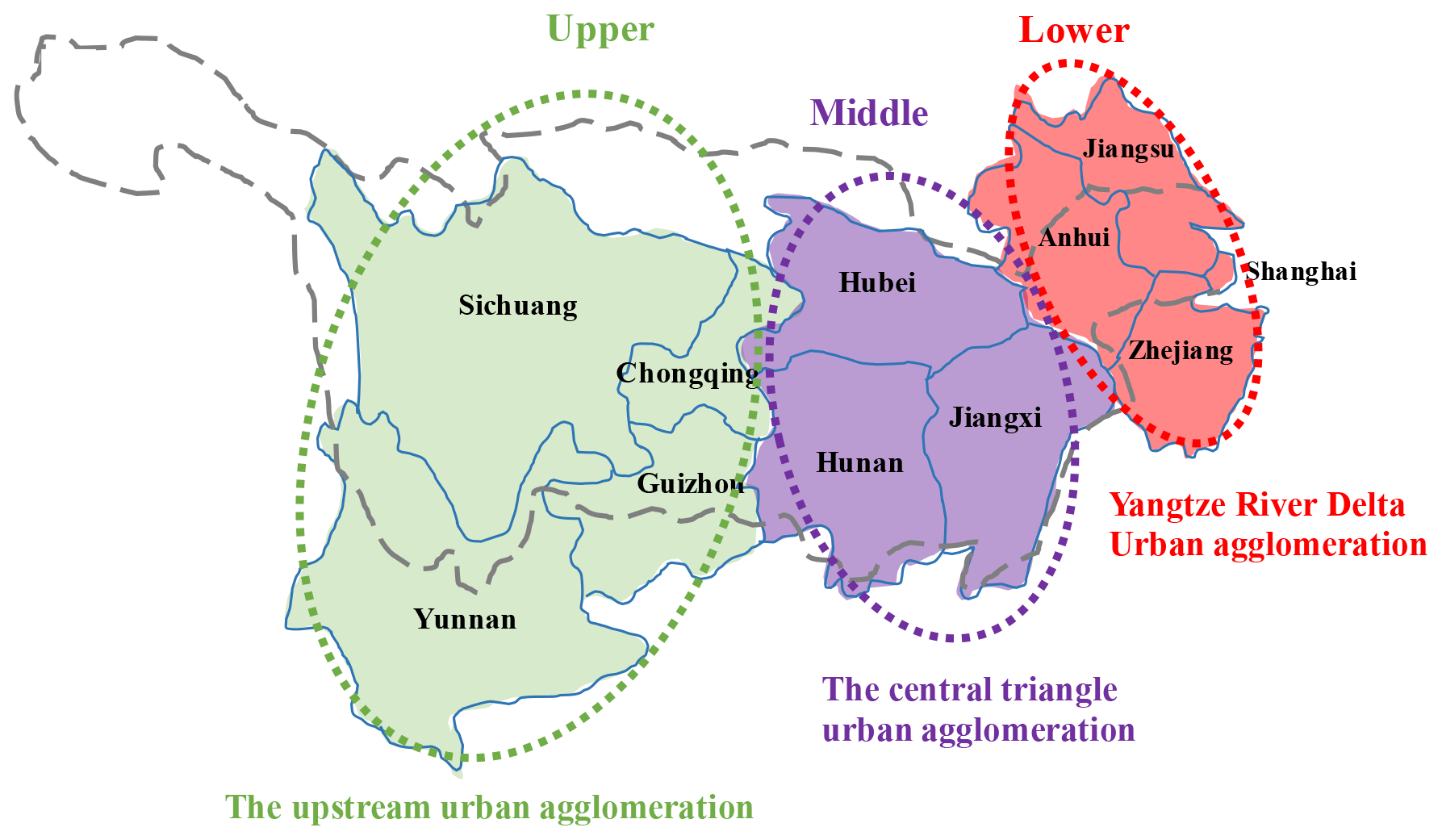
Figure 1The Yangtze River basin (long dashed black line) and the Yangtze Economic Belt.
Over the past few decades, especially after the reform and opening up of China in the late 1970s, the Belt has developed into one of the most vital regions of China. It accounts for 21 % of the country's total land area (2.05 million square kilometers) and is home to 40 % of the country's total population, with an economic output exceeding 40 % of the country's total GDP. The Belt is home to many advanced manufacturing industries, modern service industries, major national infrastructure projects, and high-tech industrial parks. As one of China's most important industrial corridors, the Belt's output from the steel, automobile, and petrochemical industries accounts for more than 36 %, 47 %, and 50 % of the total national output, respectively (MIIT, 2016). In 2018, the Belt's population and GDP were about 599 million people and RMB 40.3 trillion, accounting for 42.9 % and 44.1 % of the national total, respectively. As the initiation of government programs in the Belt in 2016 and the gradual loosening of China's birth control policy, the Belt's processes of urbanization and industrialization are expected to gain momentum in the coming decades (NDRC, 2016). The fast urbanization and strong economic growth in the Belt, however, pose severe challenges for its sustainable development. These challenges mainly include climate change impacts, energy crises, land availability, food security, water pollution, and depletion of fish stocks in the river.
2.1 Climate change impacts
The Yangtze river basin is vulnerable to global warming. Accumulating evidence shows that climate change affects the hydrologic regime in the river basin. For example, research finds that the glaciers in the Tibetan Plateau at the head of the Yangtze River shrank by 7 % (3790 km2) over the past 4 decades (Li et al., 2010). Changes in the hydrological cycle result in more frequent extreme meteorological events happening in the Yangtze rive basin (Cao et al., 2011; Gu et al., 2015; Su et al., 2017), exposing the vast majority of the population to growing physical and socio-economic risks. For example, during the summer of 2020, eight provinces in the Yangtze River basin experienced severe floods, leaving hundreds dead and disrupting the economy's post-pandemic recovery.
2.2 Energy crisis
The Yangtze river basin is poor in fossil fuel endowments even though China has the world's largest coal reserves. Data from China Energy Statistical Yearbook indicates that in 2015 the Belt imported about 60 % of its coal consumption (Department of Energy at National Bureau of Statistics, 2016). The Yangtze River basin has, however, abundant hydropower resources. The estimated hydropower potential in the river basin is about 278 million kilowatts (Wang, 2015). The Yangtze's coastal areas are an ideal location for nuclear plants. However, due to technical limitations and development costs, coal still dominates energy consumption, currently accounting for about 56 % of total energy consumption (Su, 2019).
2.3 Land availability and food security
Statistics from the Demographic Yearbook (http://www.stats.gov.cn/english/, last access: 16 May 2022) indicate that the Yangtze River basin's population grew from 500 million in 1990 to about 600 million in 2020 and is expected to reach its peak around 2030 if the one-child policy remains unchanged (Zeng and Hesketh, 2016). As the country's birth control policy gradually loosens, the population in the Belt will grow even faster. With a high population growth rate and rising income, the consumption of food, especially non-starchy food such as dairy and meat, is expected to increase (Niva et al., 2020). This higher food production has to come from the same amount of land or even less land due to the competing use of land for urbanization. Population growth and urban expansion occupy many rich farmlands. Research shows that from 2000 to 2015 urban areas in the Yangtze river basin increased by 67.51 %, whereas cropland decreased by 7.53 % (Kong et al., 2018).
2.4 Water pollution
The increasing application of fertilizers and pesticides in agriculture and discharging of wastewater from a growing population and rapid industry development lead to severe problems concerning pollution of freshwater, eutrophication of lakes, and deterioration of the water ecosystem. Statistical data indicate that 86.9 % of major lakes and 35.1 % of major reservoirs in the Yangtze River basin suffer from eutrophication (Yangtze River Water Resources Commission, 2016). Among them, the most serious case is the eutrophication of Lake Taihu, which is located in the floodplain of the lower Yangtze River (Li et al., 2011). In 2007, the blue algal bloom outbreak in Lake Taihu cut off drinking water supply for 2 million citizens in Wuxi city for a whole week (Qin et al., 2007). The last decade has witnessed around RMB 70 million flowing into the eutrophication control of Lake Taihu annually.
2.5 Depletion of Yangtze fish stock
Fishery resources in the Yangtze River are seriously depleted. To date, wild-capture fishery production decreased to less than 100 000 t, falling well short of the maximum output of 427 000 t seen in the 1950s (Zhang et al., 2020). The eggs and larvae counts for the four major Chinese carp species totaled approximately 1.11 billion in 2015, accounting for only 1 % of historical production in 1965 (Yi et al., 1988; Zhang et al., 2017). Habitat fragmentation and shrinkage as a result of reclamation of lakes for farmland and dam construction, together with overfishing and water pollution, are the main factors threatening aquatic biodiversity in the Yangtze River (Jiang et al., 2020; Zhang et al., 2020). In an effort to protect the Yangtze's aquatic life, a 10-year commercial fishing ban was introduced in 2020. Fishing in the main body of the Yangtze River, the Poyang and Dongting lakes, and the seven major Yangtze tributaries is temporarily banned for a period of 10 years starting from 2021.
The ANEMI_Yangtze model currently consists of nine sectors: population, economy, land, food, energy, water, carbon, nutrients, and fish. It is developed based on the ANEMI3 global model (Breach and Simonovic, 2021). The time horizon of the model is 2100, and the simulation step is 1 year. By introducing a subscript variable, location (consisting of of upper, middle, and lower Belt), we are able to build “one” model to account for the spatial heterogeneity within the Belt's three economic zones – the upper Chongqing–Sichuan upstream urban agglomeration, the middle central triangle urban agglomeration, and the lower Yangtze River Delta agglomeration. The model is grounded in systems-based thinking and developed using the system dynamics simulation approach. System dynamics research originates from control engineering and is a valuable methodology for capturing the nonlinearity, feedbacks, and delays in determining the dynamic behavior of complex systems (Forrester, 1961). In system dynamics, interactions and feedbacks between system components, illustrated using a causal loop diagram (CLD), are far more important for understanding system behavior than focusing on separate details (Simonovic, 2009).
3.1 Cross-sectoral interactions and feedbacks
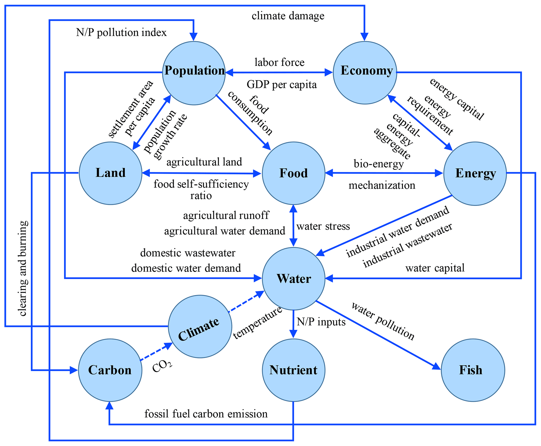
The cross-sectoral interactions and feedback in ANEMI_Yangtze (Fig. 2) are discussed in the following sections.
The population and economy sectors are linked through GDP per capita and the labor force. The population sector affects the economy sector through the labor force, an important element of the Cobb–Douglas production function. The economy sector affects the population sector both positively and negatively through GDP per capita. The reasoning behind this impact is that, on the one hand, increased economic output results in higher-quality health services and life expectancy, thereby reducing mortality rates, but, on the other hand, high housing prices accompanied by economic development usually restrains fertility choices, thus reducing birth rates (Meadows, 1974; Dettling and Kearney, 2014; Breach, 2020). In China, the total fertility in the more developed southeastern regions is generally lower than in the less developed western regions (Hui et al., 2012; Clark et al., 2020). Economic factors are the most important driver of migration (Lee, 1966). The difference in GDP per capita among the Belt's three economic zones affects population migration within the Belt.
The population, food, and land sectors are connected through population growth rate, food self-sufficiency ratio, and settlement area per capita. Population growth accelerates the transfer rate of biome among different land-use types (Goudriaan and Ketner, 1984). Population growth drives food consumption, thereby decreasing food self-sufficiency, resulting in more agricultural land being converted by clearing and burning forests and grassland. Population growth also leads to more agricultural land around the urban area be claimed for settlement use as urban expands. The land sector negatively impacts population growth, as increased population places more stress on settlement area per capita, which then acts as an opposing force on the migration rate (this feedback is further clarified in Sect. 4.3).
The economy and energy sectors are linked through a capital–energy aggregate, energy capital, and energy requirements. A growing economy increases the need for energy, which drives energy production through increasing energy capital investment. An increase in energy capital further intensifies the capital–energy aggregate, driving economy growth, thus forming a positive feedback loop.
The population, food, energy, and water sectors are connected via domestic water demand and consumption, agricultural water demand and consumption, and industrial water demand and consumption. Water plays a vital role in food production and is needed in almost every stage of energy extraction, production, processing, and especially consumption. With increased population and demand for food and energy, the total demand for and consumption of water increases, increasing water stress, which in turn impedes population growth and food production (Dinar et al., 2019; Breach, 2020). The increasing water stress also drives more capital flowing into water supply development so as to alleviate water stress, thus connecting the economy sector with the water sector.
The use of water by population, energy, and food sectors all results in water pollution in the form of increased nutrient concentration through the discharge of domestic and industrial wastewater and agricultural runoff. This links the water sector with the nutrient sector. An increased level of nutrient concentration negatively affects population growth through the life expectancy multiplier (Pautrel, 2009), and this thus links the nutrient and population sectors. Water pollution also endangers fish by increasing the population's natural mortality rate (Zhang et al., 2020).
The carbon and land sectors are connected through clearing and burning, while the carbon and energy sectors are connected through fossil fuel emissions. The carbon–climate sector feedback depends on the atmospheric CO2 concentration determined by the carbon sector. The climate change effect is treated exogenously. The climate and water sectors are connected via surface temperature change. Since increased surface temperature will likely increase the intensity of hydrological cycle (Giorgi et al., 2011), the model includes a temperature multiplier equation that increases evaporation and evapotranspiration. The climate sector influences the economy sector through a temperature damage function developed by Nordhaus and Boyer (2000).
3.2 Interactions and feedbacks within model sectors
3.2.1 CLD in the population sector
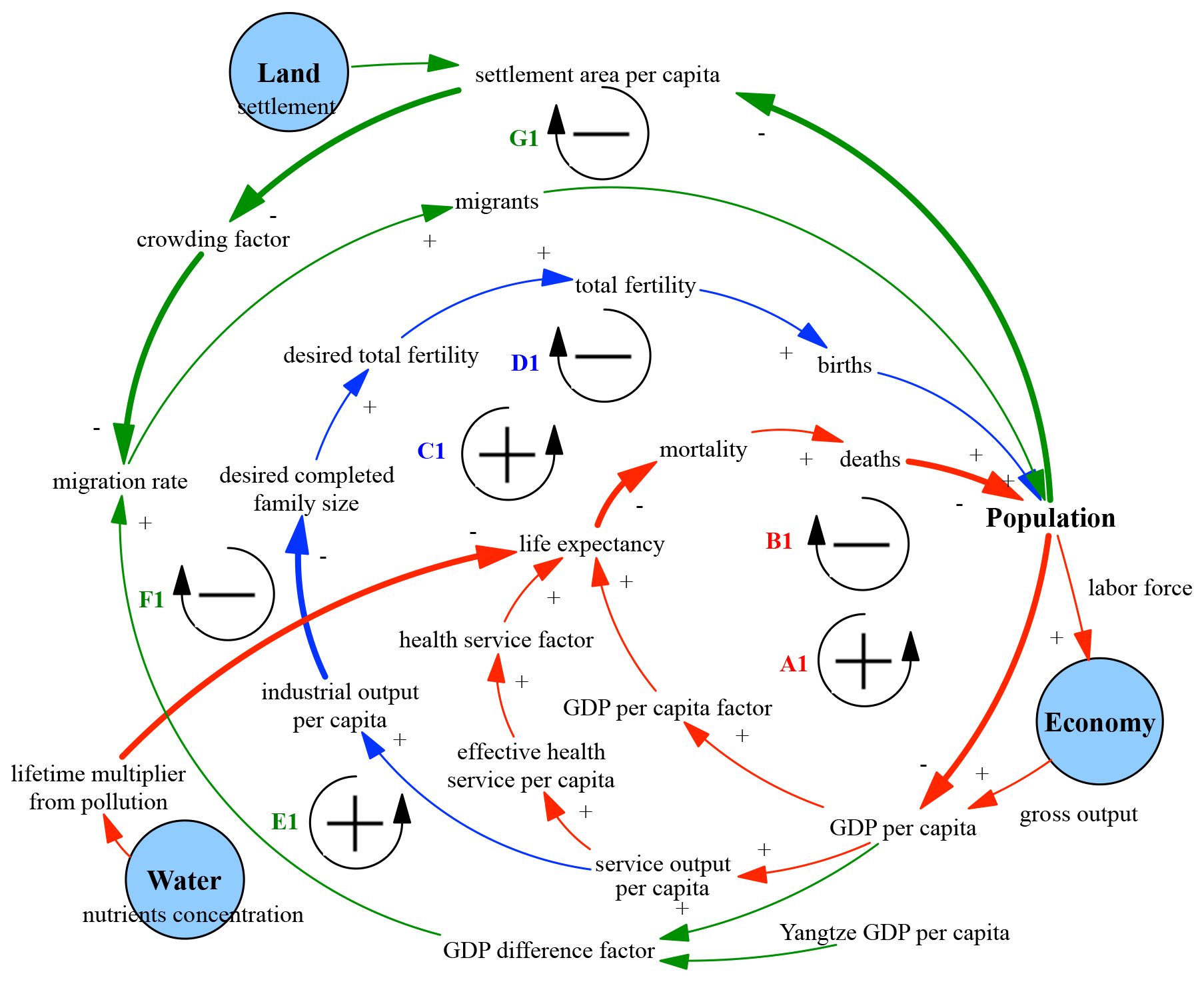
Three variables, i.e., births, deaths, and migrants, which are all affected by GDP per capita, drive the dynamic behavior of the population in the Belt. GDP per capita is affected by labor force and gross output and rises if the effect of the increase in the gross output outpaces the effect of the population increase and vice versa. Thus, any loops containing GDP per capita can either be positive or negative depending on whether it is increasing or decreasing with population growth. Figure 3 shows the feedbacks in the population sector. The positive loop A1 and negative loop B1 depict the effect of GDP per capita on mortality, whereas positive loop C1 and negative loop D1 show the same for fertility. The positive loop E1 and negative loop F1 illustrate the impact of GDP difference factor on migration, whereas loop G1 explains the effect of crowding on migration. The process of (and mechanism behind) the CLD is illustrated in Sects. 3.1 and 4.3.
3.2.2 CLD in the economy sector
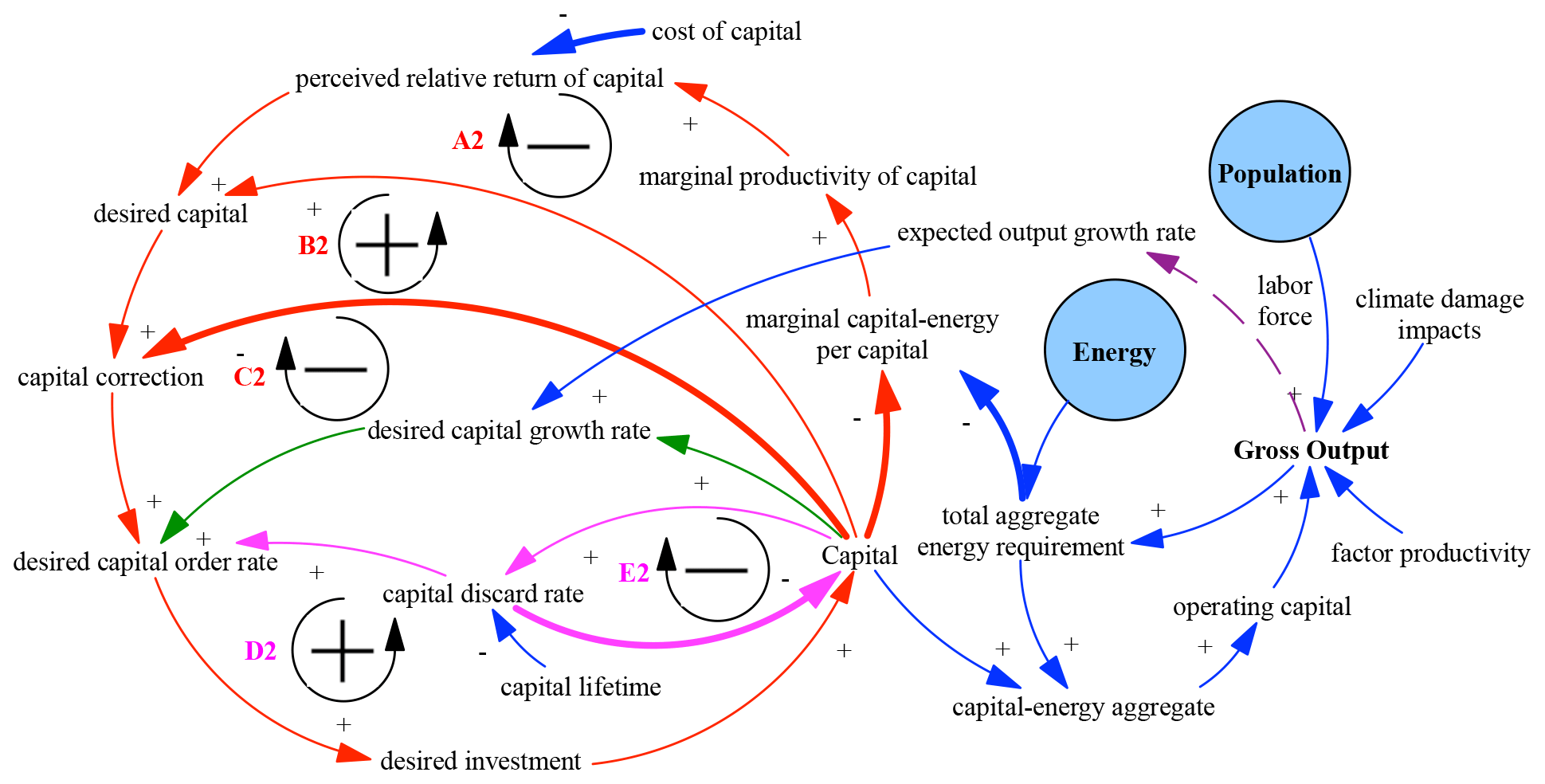
Figure 4 displays the interactions and feedbacks in the economy sector. Capital orders respond to three pressures. Orders first replace depreciation (loops D2 and E2). Loop E2 depicts the process of depreciation, which slowly depletes capital stock. Loop D2 compensates for depreciation by factoring it into the desired capital order rate. Orders then correct the gap between desired and actual capital (loop C2). Desired capital stock is anchored on real capital stock and adjusted for relative cost and marginal product of capital (loops A2 and B2). Finally, orders augment capital stock in order to anticipate output growth. See also Fiddaman (1997) and Breach (2020) for more information about the detailed process of (and mechanism behind) the CLD in the economy sector.
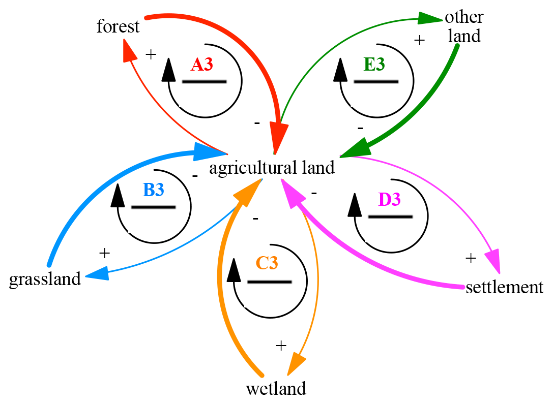
3.2.3 CLD in the land sector
Figure 5 illustrates the feedbacks for agricultural land (the feedback in the forest, grassland, wetland, settlement, and other land categories, which are not shown in Fig. 5, are the same as those in the agricultural land). An increase in the stock of agricultural land increases its transfer rate to the forest, grassland, wetland, settlement, and other land categories, which together drain the stock of agricultural land and form the negative loops A3, B3, C3, D3, and E3.
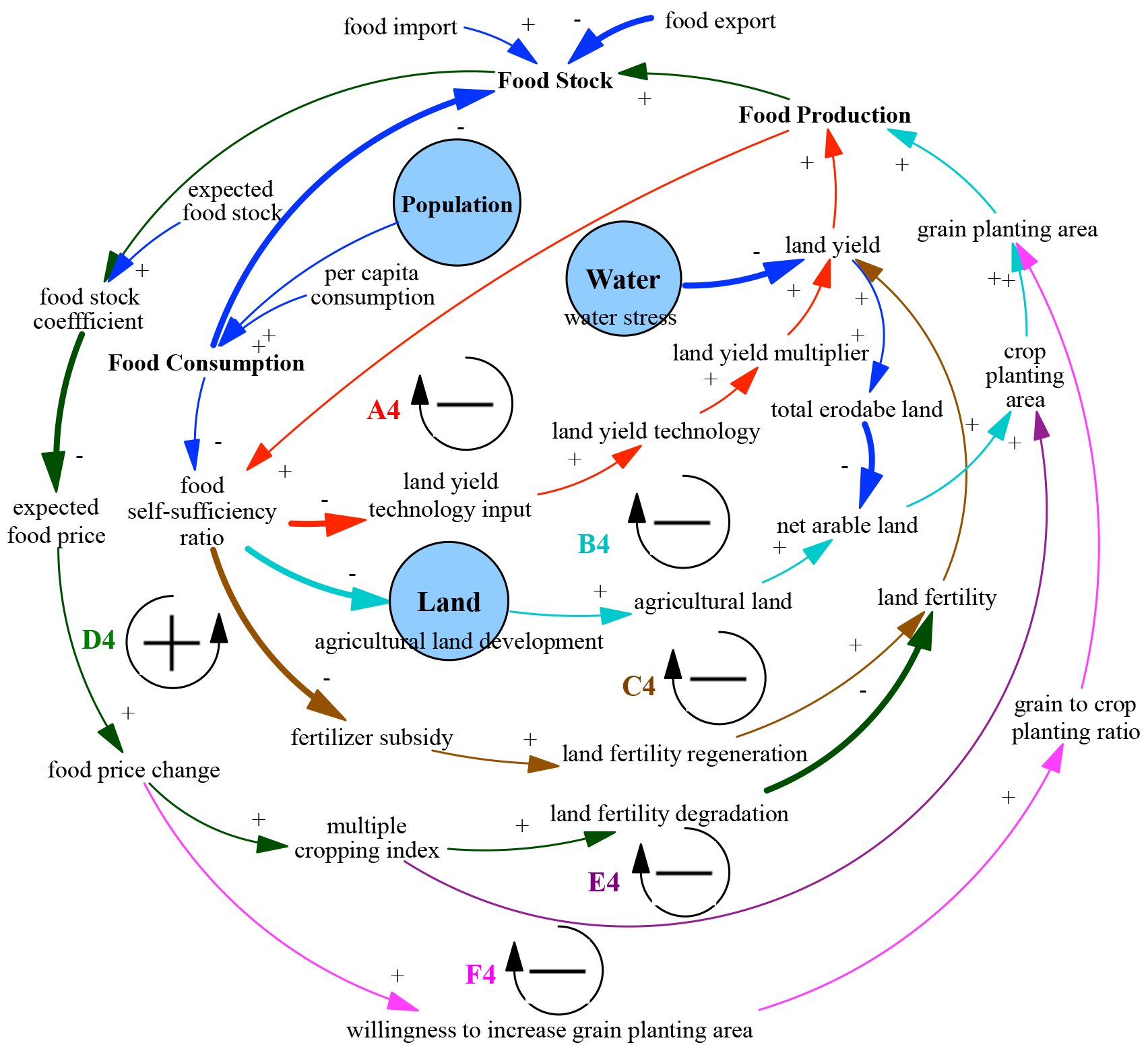
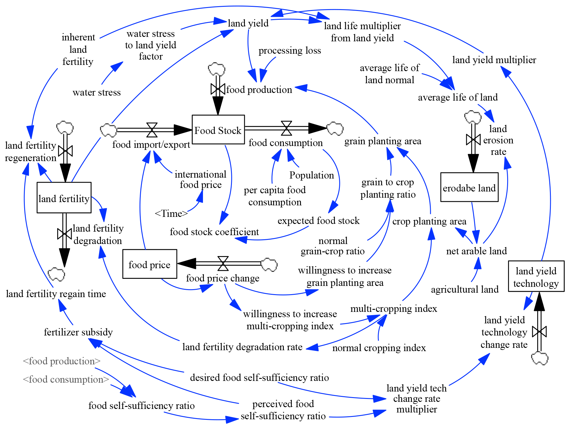
3.2.4 CLD in the food sector
Figure 6 shows the CLD in the food sector. Negative loops A4, B4, and C4 illustrate the impacts of land yield technology, agricultural land development, and fertilizer subsidy, respectively, on food production through the food self-sufficiency ratio indicator. A decrease in food self-sufficiency ratio stimulates inputs in land yield technology, agricultural land development, and fertilizer subsidy, which all drive up land yield, resulting in increases in food production and food self-sufficiency ratio (Ju et al., 2020). Changes in agricultural product prices are recognized as significant factors driving grain production (Xie and Wang, 2017). Negative loops E4 and F4 depict the introduction of multiple cropping practices (multiple cropping index) and the willingness to increase the grain planting area for food production through food price change. An increase in food price change acts as positive feedback on farmers' adopting of multiple cropping practices (multiple cropping index) and increasing their grain planting area. Positive loop D4 counterbalances the effect of adopting multiple cropping practices by decreasing land fertility and the corresponding land yield.
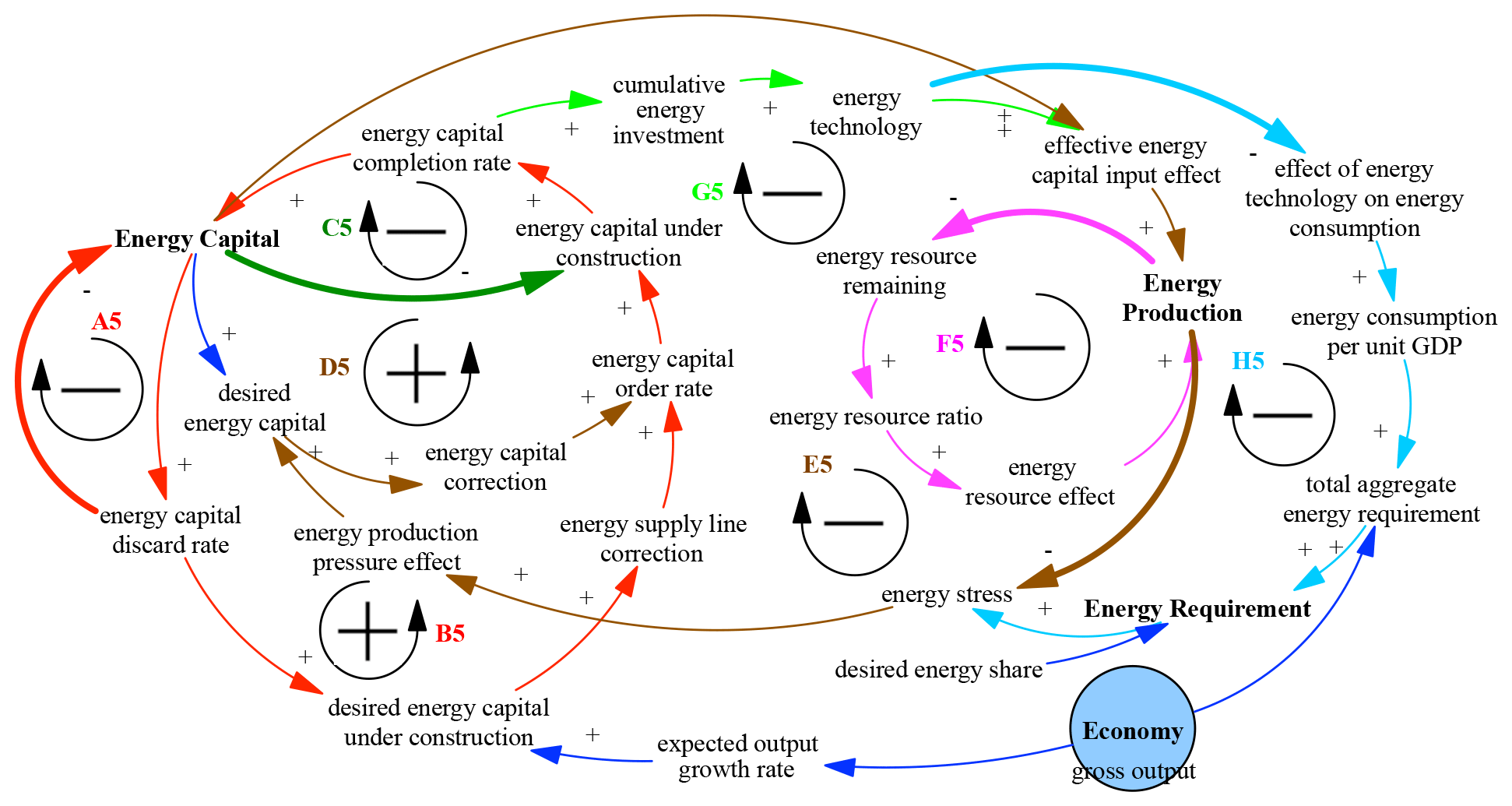
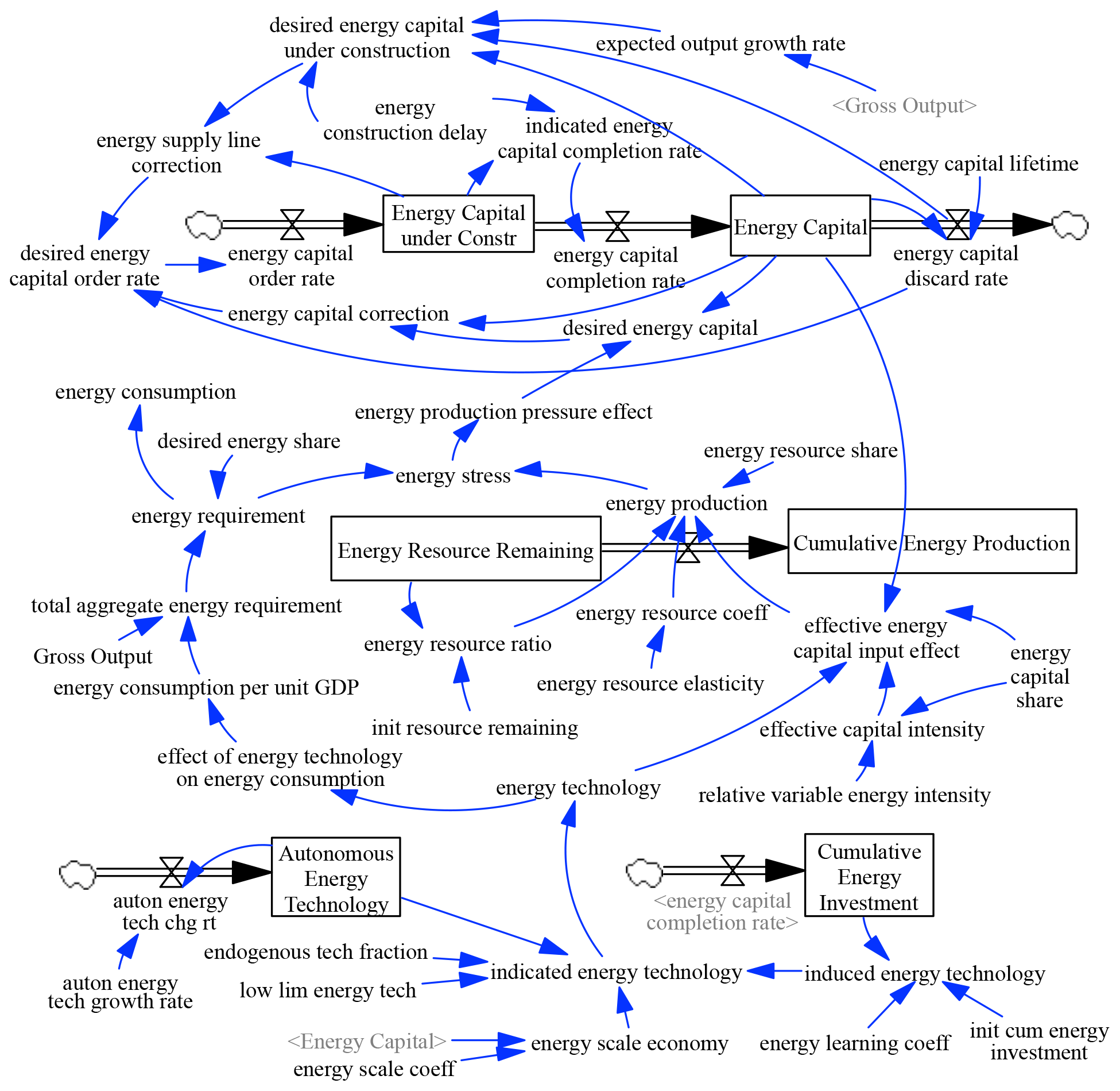
3.2.5 CLD in the energy sector
Figure 7 shows the CLD in the energy sector. Energy capital orders respond to two pressures. Orders first replace depreciation (loops A5 and B5). Loop A5 depicts the process of depreciation, which slowly depletes energy capital stock. Loop B5 compensates for depreciation by factoring it into desired energy capital under construction. Loop C5 moves energy capital from the construction phase to the completion phase. Orders then correct the gap between desired and actual energy capital (loop D5). Desired energy capital stock is anchored on actual energy capital stock and adjusted for energy production pressure (E5, which depicts the effect of energy production pressure on energy capital). Technology plays essential role in the energy sector. Energy technology, on the one hand, increases energy production for the same level of input of energy capital (loop G5) but, on the other hand, significantly lowers the intensity of energy consumption per unit of GDP (loop H5). Loop F5 illustrates the impact of resource depletion on energy production. Energy resources gradually deplete as more energy is produced. See also Fiddaman (1997) and Breach (2020) for more information about the detailed process of (and mechanism behind) the CLD in the energy sector.
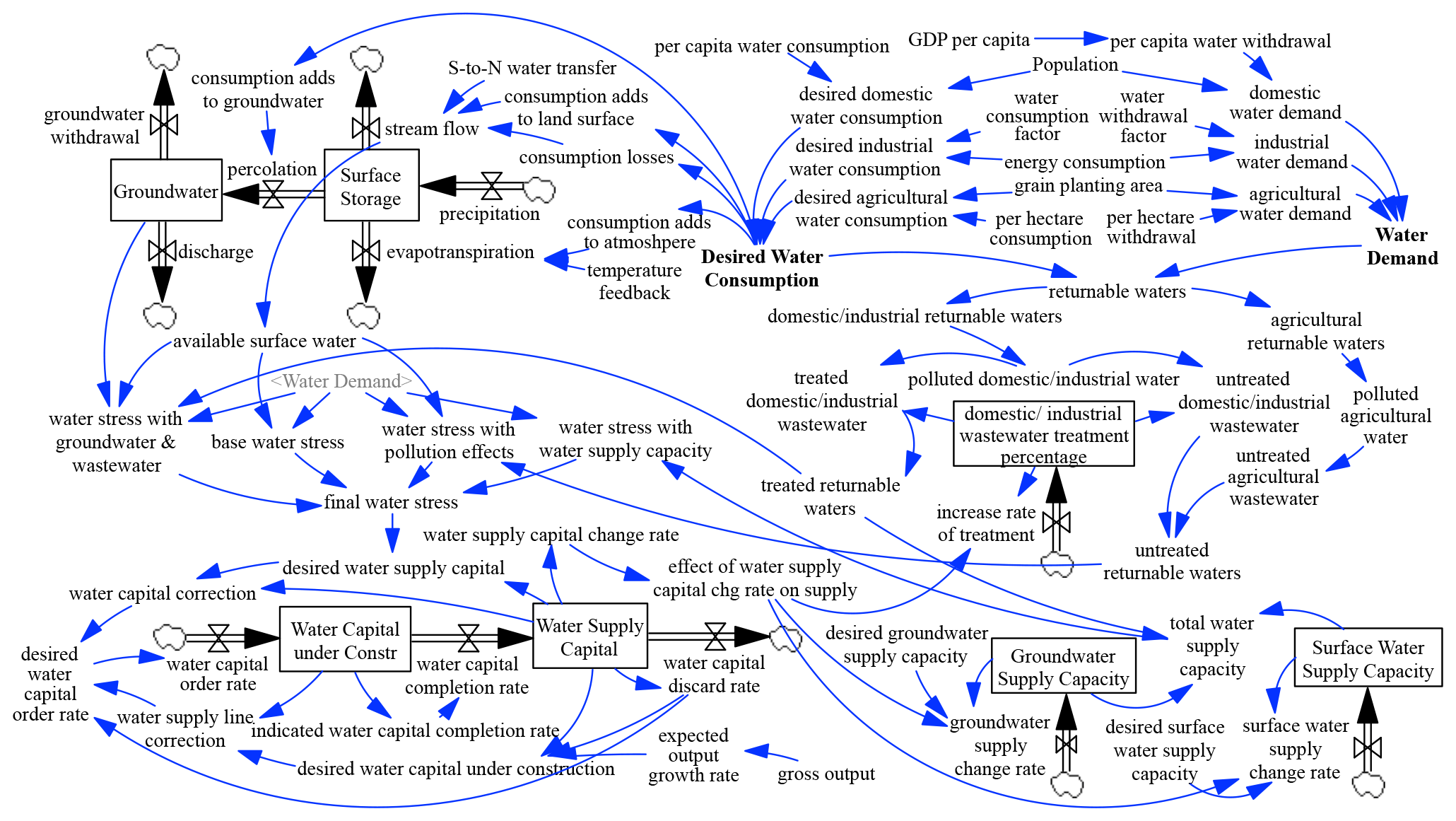
3.2.6 CLD in the water sector
Figure 8 shows the CLD in the water sector. Water supply capital orders respond to three pressures. Orders first replace depreciation (loops A6 and B6). Loop A6 depicts the process of depreciation, which slowly depletes water supply capital stock. Loop B6 counteracts loop A6 by factoring it into desired water capital order rate. Orders then correct the gap between desired and actual water supply capital. Desired water supply capital stock is anchored on actual capital stock and adjusted for water stress (loops C6, D6, and E6). Loops C6, D6, and E6 counteract water stress by prompting investment in water supply capital to increase water supplies in the form of surface water, groundwater, and treated returnable waters, respectively. Finally, orders augment water supply capital stock in order to anticipate output growth. Loop F6 illustrates the movement of water from the atmosphere to the surface as precipitation and then back to the atmosphere through evapotranspiration. Loop G6 depicts the effect of discharge on groundwater. See also Breach (2020) for more information about the detailed mechanism behind the CLD in the water sector.

3.2.7 CLD in the carbon sector
Figure 9 shows the CLD in the carbon sector. The chain of negative loops passing through each of the terrestrial carbon stocks from the biomass to litter, to humus, and to stable humus and charcoal (A7, B7, C7) and the negative loops depicting the decaying (E7, G7, H7, I7) and burning (D7, F7) process of each carbon stock all act as a positive loop in the atmosphere–terrestrial carbon cycle (K7 and J7). An increase in atmospheric carbon results in higher uptake of carbon in the biomass through the effect of net primary productivity, which results in a greater transfer of carbon through the chain (biomass, litter, humus, stabilized humus and charcoal), thereby leading to an increase in decay and transfer of carbon back to the atmosphere. See also Goudriaan and Ketner (1984), Davies and Simonovic (2010, 2011), and Breach (2020) for more information about the detailed mechanism behind the CLD in the carbon sector.

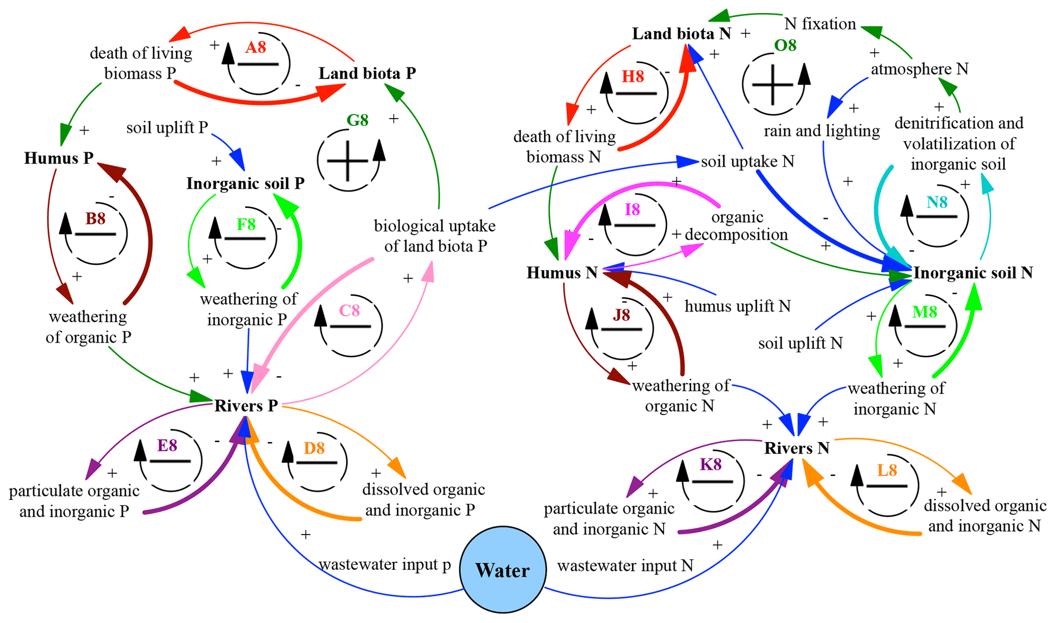
3.2.8 CLD in the nutrient sector
Figure 10 shows the CLD in the nutrients sector. The cycles of phosphorous and nitrogen follow that of the carbon cycle. Take a phosphorous cycle for example, the chain of negative loops passing through land biota to humus and to rivers (A8, B8, C8, D8, E8) and the negative loops depicting the weathering of inorganic P (F8) act as a positive loop in the terrestrial phosphorous cycle (G8). Because it represents a continuous cycle of negative feedback, it will attempt to reach equilibrium under natural conditions. Anthropogenic influences on this system in the form of wastewater discharge affect this equilibrium and drive changes in the nutrient cycles. See also Mackenzie et al. (1991) and Breach (2020) for more information about the detailed mechanism behind the CLD in the nutrient sector.
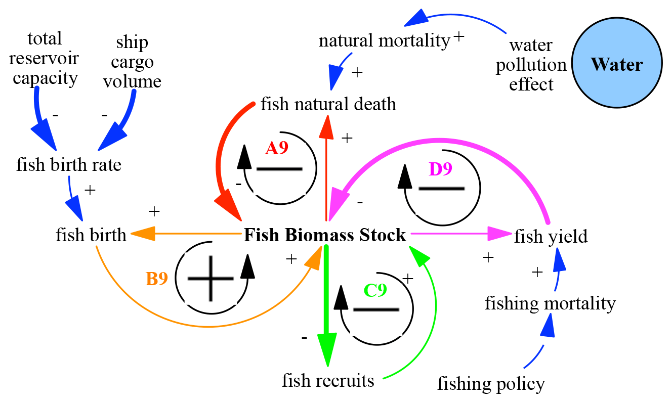
3.2.9 CLD in the fish sector
Four feedback loops drive the dynamics of fish biomass stock (Fig. 11). Loops A9, C9, and D9 represent negative feedback on fish biomass stock through natural fish death, fish recruits, and fish yield, respectively. The amount of wastewater water acts as a positive factor on natural mortality. Loop B9, which connects total reservoir capacity and ship cargo volume with fish birth rate, acts as positive feedback on fish biomass stock. As total reservoir capacity and ship cargo volume increase, fish birth rate and total fish births decrease. The decline in fish births decreases fish biomass stock, further reducing fish births.
4.1 The ANEMI_Yangtze data system
The ANEMI_Yangtze data system contains (i) historical data that are used to initialize and validate the model and (ii) future parameters that govern changes in the future. Most of the historical data (1990–2015), such as population and GDP, energy production and consumption, food production and food trade, and water withdrawals and consumptions, come from the Statistical Yearbook published by the National Bureau of Statistics of China (available online at http://www.stats.gov.cn/english/, last access: 16 May 2022). Historical precipitation, evapotranspiration, and temperature data are collected from hydrometeorological stations. Land use data come from ESA Climate Change Initiative – Land Cover (http://maps.elie.ucl.ac.be/CCI/viewer/, last access: 16 May 2022). Adjustments are made to the historical data as needed to fill in the missing information. Future temperature and precipitation data come from Yu et al. (2018). For future parameters, the ANEMI_Yangtze data system uses information about technology cost and performance, information about future development policies, and the authors' experience and knowledge. Additional information about the data is also given in the sections below.
4.2 Major changes: a glimpse
ANEMI_Yangtze is developed based on ANEMI3, which has its roots in the WorldWater model by Simonovic (2002a, b). ANEMI has been updated continuously from its first publication in 2010 (Davies and Simonovic, 2010) to the most recent edition in 2021 (Breach and Simonovic, 2021). The current version of ANEMI consists of the following 12 sectors that reproduce the main characteristics of the climate, carbon, population, land use, food production, sea level rise, hydrologic cycle, water demand, energy economy, water supply development, nutrient cycles, and persistent pollution. In ANEMI_Yangtze, hydrological cycle, water demand, water supply development, and wastewater discharge and treatment are all integrated into the water sector. Climate change is not explicitly simulated. Instead, we use exogenous precipitation and temperature to drive the hydrological cycle. Sea level rise and persistent pollution are excluded. The global cycles of carbon, nutrients, and hydrology are tailored to fit a regional context. A new fish sector is added since fisheries are important for regional economy and diet. Major modifications are made to the population, food, energy, and water sectors. Due to space limitation, only new aspects of the model are described in detail. For further information about the model, please refer to ANEMI_Yangtze's technical report from Jiang and Simonovic (2021) and the PhD dissertation of Breach (Breach, 2020).

4.3 Population
Births, deaths, and migrants are the three variables drive the dynamic behavior of the Belt's population. Figure 12 shows the stock and flow diagram in the population sector. Population is split into three age demographics to allow for working population (ages 15 to 64) to represent the labor force in the economic model. The aging chain of population groups can be represented as follows:
where Pi is population, netMi is net migrants, Mi is mortality, and τi is the length of time spent in each sub-demographic. B represents births and is calculated as follows:
where FMr is the female-to-male ratio (its value is usually lower than 0.5 due to the well-known phenomenon of “missing girls”, a side-effect of the one-child policy), P15−49 is the population between age 15–49, and Rlife is reproductive lifetime of 30 years. TF is total fertility, which is determined by a number of factors, including fertility control effectiveness, capital allocation, and desired family size. Its calculation (Eq. 3) is adapted from ANEMI3 (Breach, 2020).
where TF is total fertility, MTF is maximum total fertility, Fcontrol is fertility control effectiveness, and DTF is desired total fertility.
Life expectancy, which determines mortality, is affected by both economic and environmental factors. The calculation of life expectancy is adapted from Ma and Yu (2009). At the regional scale, vital resources such as food and water can be traded, and thus in ANEMI_Yangtze only the effect of pollution is considered. The empirical relationship between mortality and life expectancy is adopted from ANEMI3, which was originally adopted from Meadows (1974).
where LE is life expectancy, LEN is life expectancy normal, GDPper is GDP per capita, EHSper is effective health service per capita, pollutionmulti is lifetime multiplier from pollution, and PI is pollution index. NI (PI) and N10 (P10) are the simulated and initial nitrogen (phosphorous) concentration. a, b, c, d, and e are calibrated parameters.
Migration is newly added. According to Lee (1966), economic factors are mainly responsible for migration. In China, the most important factor driving migration in the 1980s (post-reform period) is the institutional driver and then the economic driver dominates afterwards (Shen, 2013). Apparently, policy on migration cannot be ignored considering China's central planning logic and mechanisms. We thus introduce a migration policy factor to account for the institutional barrier and suppose that its value ranges from 0–1, with higher values indicating policy that is in favor of migration. Social environment is also an intermediate factor affecting migration (Lei et al., 2013). In China, most minorities (China's 56 ethnic groups) live in areas with the same (or similar) language, culture, and eating habits and are very reluctant to move (Su et al., 2018). Therefore, we employ a factor – migration willingness – which is calculated as the proportion of the minorities to account for the “border effect” in migration. Research also finds that economic prosperity not only attracts labor migration but also restrains population inflows in megacities due to high housing prices (Zhao and Fan, 2019). This research introduces a crowding factor affected by settlement area per capita to account for house price impact. The calculation of migration rate MR is thus formulated as follows:
where FGDP diff is GDP difference factor, which is used to calculate the difference between GDP per capita in the upper, middle, and lower Yangtze Economic Belt and GDP per capita in the Belt. This means only the migration within the Belt is considered (i.e., people migrate from the less developed upper and middle Belt to the developed lower Belt). MW is migration willingness. MP represents migration policy, and a value of 1 is adopted in this research. Fcrowding is a crowding factor and is affected by settlement area per capita.
4.4 Food
The food sector of ANEMI_Yangtze calculates the production and consumption of food and food import/export, and its stock and flow diagram is shown in Fig. 13. Food consumption is the production of population and per capita food consumption. In ANEMI_Yangtze, per capita food consumption is assumed to be 400 kg per year per person throughout the simulation. Food production is affected by several factors, including land fertility, arable land, and water stress. Its dynamic behavior is mainly driven by the difference between perceived and desired food self-sufficiency. The food self-sufficiency index is defined as the ratio of food production to food consumption. When its value declines below 0.95 (a critical value) incentives for land yield technology input, agricultural land development, and fertilizer subsidy shall be provided to ensure food security (Ye et al., 2013).
where FP is food production, LY is land yield, GPA is grain planting area, and loss represents processing loss. LF is land fertility, LYmulti is land yield multiplier, and FWS represents water stress to land yield factor.
The food sector also enables food trade, i.e., food import and food export, which is affected by local food price and international food price, and its calculation is adapted from Wang et al. (2009).
where FIE is food import/export, with positive FIE indicating import and negative FIE representing export. Fpop is population rescale factor, approximately equal to the ratio of the Belt's population to the national total population. FP is food price and IFP is international food price. The historical values of IFP are from FAO (http://www.fao.org/worldfoodsituation/foodpricesindex/en/, last access: 16 May 2022). The future values are set to the base year 2015 values. fi is calibrated parameter. Food price is simulated as a stock variable and accumulates via food price change, which is another important factor affecting food production through influencing farmers' adopting of multiple cropping practices (multiple cropping index) and increasing of grain planting area.
4.5 Energy
The energy system of ANEMI_Yangtze includes the representation of energy capital development; energy technology; and energy requirement, production, and consumption. Figure 14 shows the stock and flow diagram of the energy sector. Six primary energy resources, three renewable (hydropower, nuclear, and new energy sources) and three non-renewable (coal, oil, and gas), are considered. Energy capital is energy production capital stock. It is represented as developed fields or mines for fossil fuels and built plants for nuclear power and hydropower. The formulations of energy capital (KEi) and energy capital under construction (KECi) are the same as those in ANEMI3 (Breach, 2020: Eqs. 3.52), 3.53). For simplicity, we do not simulate the effect of return on energy capital, which is determined by energy capital cost and the marginal product of energy capital in ANEMI3. We thus formulated the calculation of desired energy capital order rate as follows:
The first term on the right-hand side of the formula represents energy capital discard rate in which KEi is energy capital and δi is energy capital lifetime. The middle term represents energy capital correction, in which DKEi is desired energy capital and is equal to current capital adjusted for production pressure. The pressure effect of energy production is treated as a lookup table function of energy stress. Energy stress is defined as the ratio of energy requirement to energy production. τc is correction time for energy capital. The third term represents correction to the supply line of energy capital under construction in which DKECi and KECi are desired and current energy capital under construction. DKECi is the quantity needed to replace discarded values and meet growth and is formulated as Eq. (12), in which GRGDP is expected growth rate of gross output and delayC represents the time required to construct new energy capital. τs is correction time for the supply line of energy capital under construction, and i denotes the six energy sources.
The total aggregate energy requirement in ANEMI_Yangtze scales with economy and is represented as the production of gross output and energy consumption per unit of GDP. Energy requirement by sources is the production of total aggregate energy requirement and desired energy share (which is exogenously specified).
Three factors affect energy production for each source: energy capital, energy technology, and resource effects. The supply of producing capital is mainly driven by the pressure effect of energy production, i.e., energy stress (defined as the ratio of energy requirement to energy production). Resource effects affect energy production through depletion and saturation. The depletion effect represents the diminishing productivity of non-renewable energy production as the resources remaining decline, and saturation refers to diminishing returns to production effort for the renewable energy. Technology increases energy production for the same level of inputs of energy capital through a learning process usually referred to as the endogenous learning curve, with cumulative investment in energy capital as its input. The formulation of energy production is the same as in ANEMI3 (Breach, 2020: Eq. 3.49), which is based on Fiddaman (1997).
Energy price in ANEMI3 is endogenously simulated, whereas in ANEMI_Yangtze it is exogenously specified, with historical prices taken from the China Customs Head Office and China Energy Statistical Yearbook and future prices assumed to remain at their 2015 base year values.
Energy consumption is equal to energy requirement by assuming that the requirements can always be met through production and trade. Energy trade is not simulated in this research.
Table 1 shows the endowments of the six energy sources. Reserves for renewables mean the upper limit to renewable output. The upper limit for hydropower is based primarily on the hydro endowment, nuclear potential is implicitly assumed to be politically limited, and new energy is the sum of potential outputs of wind and solar energy.
Table 1Energy endowments in the Belt (tce: ton of standard coal equivalent, 1 tce = 29.3 billion joules).

4.6 Water
The water sector consists of the hydrological cycle, water demand, desired water consumption, water supply development, and wastewater discharge and treatment. Figure 15 shows the stock and flow diagram of the water sector.
The hydrological cycle describes the flow of water from atmosphere in the form of precipitation to land surface storage and through groundwater back to East China Sea. The south-to-north water transfers (west, middle, and east lines) and water consumption are also considered. The water balance equations in the Belt are as follows:
where SS is surface storage, Pre is precipitation, and ET is evapotranspiration. Per and SF represent percolation and stream flow and are formulated as in Eqs. (15) and (16), respectively. CSat, CSls, CSgr, and CSloss represent the water that consumption adds to atmosphere, land surface, groundwater, and consumption loss, respectively. S2N is the south-to-north water transfer; a, b, and c are calibrated parameters. GW is groundwater, GWW represents water withdrawn from groundwater storage, and Dis means groundwater discharge and is formulated as Eq. (17).
The calculation of domestic and agricultural water demands and consumption is the same as in ANEMI3. Industrial water demand is dominated by the generation of electricity, which consists of both non-renewable sources (coal-fired and gas-fired thermal power) and renewable sources (hydropower and nuclear power). The water withdrawal factor and water consumption of thermal energy both vary substantially among different cooling methods, and their values for different fuel sources are obtained from Zhang et al. (2016) and shown in Table 2. Nuclear power plants in the Belt are located in coastal areas and rely on seawater for cooling, so the freshwater withdrawal and consumption factors of nuclear power are all set to zero. The calculation of electricity water demand takes the following form:
where Wele is electricity water demand, is electricity production for energy source i, WWFi is water withdrawal factor for energy source i, Fi,j is the fraction of cooling method j for energy source i and is externally prescribed, and Techele is technological change for withdrawals in electricity production and is also exogenously specified. Industrial water demand is calculated as follows:
where Wind is industrial water demand and Rele is the ratio of electricity water demand to industrial water demand and is set to 0.7 in this research.
Table 2Water withdrawal and consumption factors for electricity production.
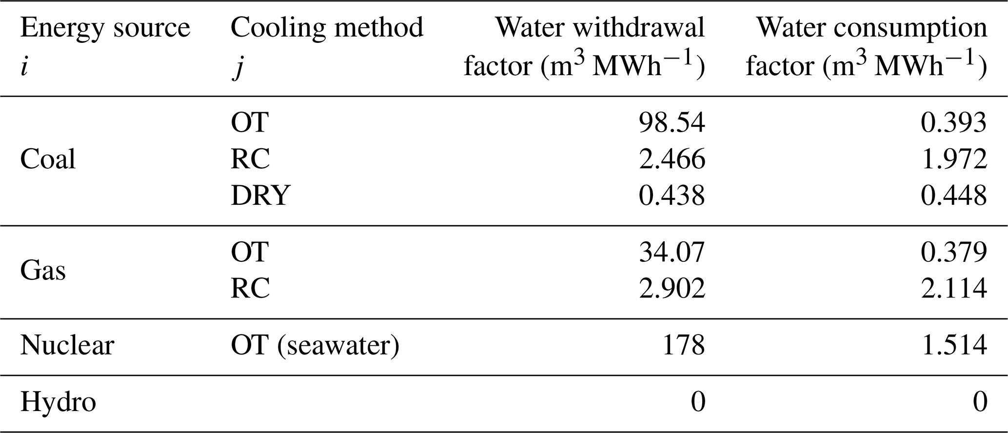
OT stands for once through, and RC stands for recirculating
In ANEMI_Yangtze, water demand is defined as the amount of water needed for the domestic, industrial, and agricultural sectors. We calculate water consumption as the desired consumption while assuming that consumption and withdrawal can always be met, which means we do not simulate the unsatisfied demand directly. Instead, we use water stress as a measure of water shortage. The definitions and formulations of water stress are described in the following sections.
Three supply types are considered: surface water, groundwater, and wastewater reclamation. The production of water supplies is driven economically by investing in water supply capital stocks for each source. The structure and formulation of water supply development follow that of the energy capital development. Similarly, the effect of water stress is introduced as an indicator for water supply capital investment and has four definitions (a value bigger than 1 indicating water shortage). The base water stress WSbase is represented as follows:
where SWavai is available surface water, which is the stable and reusable portion of the total renewable streamflow.
The water stress with groundwater and wastewater WSgw+ww is represented as follows:
where rgw is groundwater use ratio, which is set to 0.01 based on the ratio of historical groundwater withdrawals to total withdrawals. GW stands for groundwater, and TRW stands for treated returnable waters.
The water stress with pollution effects WSpollution is represented as follows:
where fww is wastewater pollution factor, which is set to 8 (based on Shiklomanov, 2000) and UTRW is untreated returnable waters.
The water stress with water supply capacity WSsupply is represented as follows:
where TWS is total water supply capacity, which is the sum of surface water supply capacity, groundwater supply capacity, and treated returnable waters.
4.7 Fish
The fish sector, which is an entirely new addition to ANEMI_Yangtze, is used to simulate the dynamic of fish biomass stock over time. Figure 16 shows the stock and flow diagram of the fish sector.
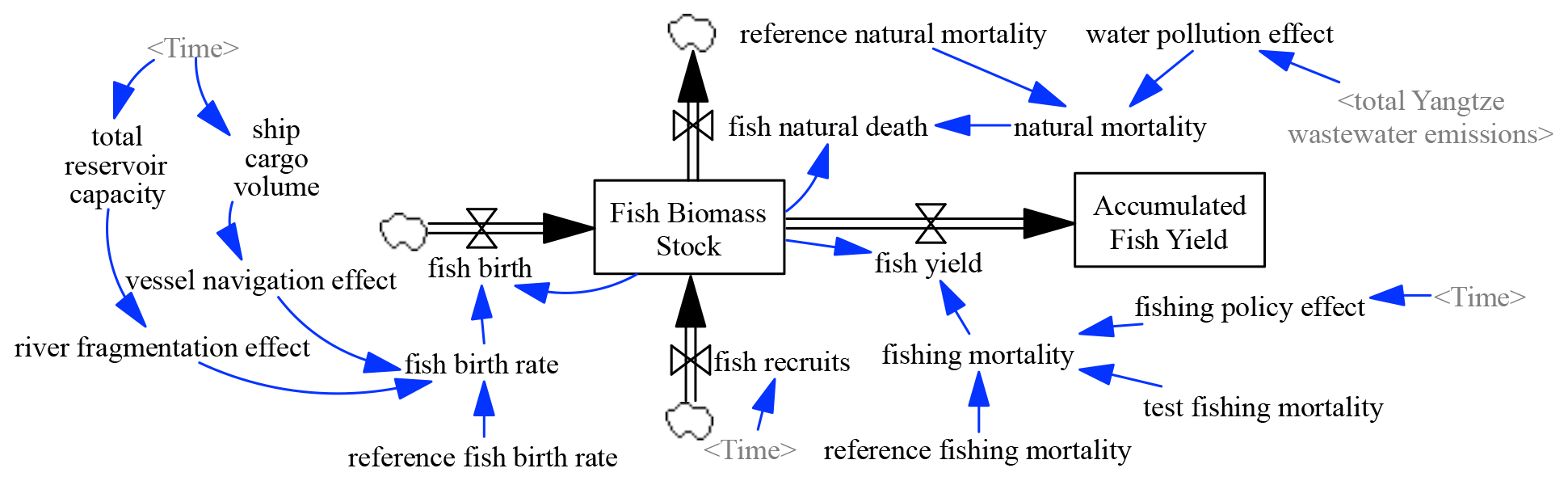
The calculation of fish biomass stock is given as follows:
where F is fish biomass stock and fb is fish birth. fr represents fish recruits, which is treated as an exogenous variable. fd is natural fish death, and fy is fish yield.
Fish catch data come from Zhang et al. (2020). Major parameters in the fish sector are given in Table 3.
Table 3Major parameters and their corresponding values in the fish sector.
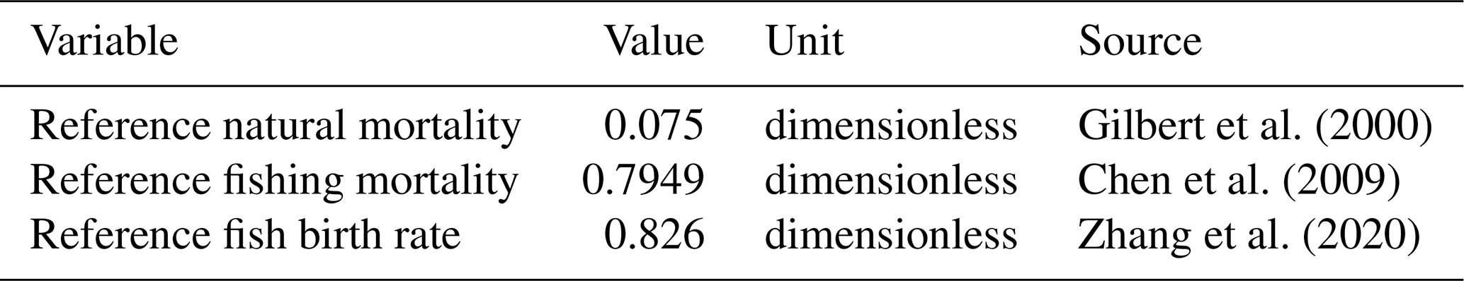
Note that for reference fishing mortality the value of 0.7949 is calculated based on Chen et al. (2009) by averaging the exploitation coefficients of 10 economic fish species (fishing mortality =0.761, 0.706, 0.803, 0.829, 0.898, 0.876, 0.846, 0.774, 0.765, and 0.691). For reference fish birth rate the value of 0.826 is calculated based on Zhang et al. (2020) by averaging fish growth rates in the middle Yangtze reach, Dongting lake, and Poyang lake.
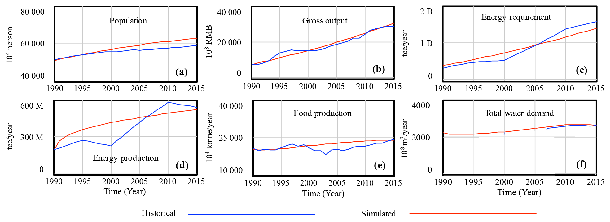
5.1 Model validation and sensitivity analysis
The ANEMI_Yangtze model was validated by comparing simulated results with historical data for 1990–2015. The results shown in Fig. 17 indicate that the model can reproduce the system behavior very well for population, gross economic output, and water demand (Fig. 17a, b, and f, respectively). The model can capture the general behavior patterns for energy requirement, energy production, and food production (Fig. 17c, d, and e, respectively). The fluctuations of historical food production are mainly attributed to the flood and drought disasters, which are not currently captured by the model. The discrepancies between historical and simulated energy requirement and energy production are partly due to the previous energy policies acting on the energy system that the model does not consider. For example, in China overcapacity in coal production gradually appeared after the mid-1990s, and this situation worsened after the outbreak of the 1997 Asian financial crisis. To alleviate the overcapacity crisis, the governments at all levels issued series of policies to reduce production, which is seen as a production drop around the year 2000 (Fig. 17d).
Sensitivity analysis aims to build confidence in the model's ability to generate robust system behavior by applying a Monte Carlo simulation. The parameters used for sensitivity tests (shown in Table 4) are chosen due to uncertainty in their values. The selected parameters are varied by −10 %–+10 % (mild-variation scenario) and −50 %–+50 % (extreme-variation scenario) to determine whether the main state variables will exhibit alternative behavior. Triangular probability distribution is used. The highest point of probability in the triangle is assigned to the baseline value of these parameters, where the outer limits are defined by the minimum and maximum percent changes of the value.
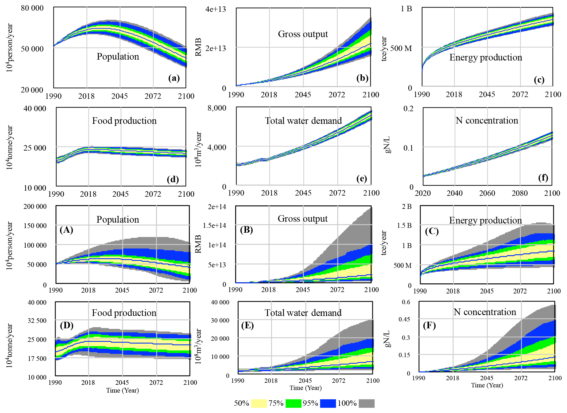
The sensitivity simulations are performed by considering all the possible parameter change combinations together, and the results are shown in Fig. 18. The lowercase letters show the results for the mild-variation scenario and the capital letters for the extreme-variation scenario. As can be seen, the range of the projected variables becomes smaller with the decreasing of the confidence level. For each of the examined variables shown in Fig. 18a–f, the behavior modes remain the same within the range of the parameters tested when the variation is mild (−10 %–+10 %). When the variation is extreme (−50 %–+50 %), the range in the trajectory of the state variables is larger. However, the behavior of each variable still remains the same (Fig. 18a–f). The lack of changes in behavior modes while testing sensitivity is desirable, indicating that the model is robust.
Table 4Parameters used for sensitivity tests of main state variables.
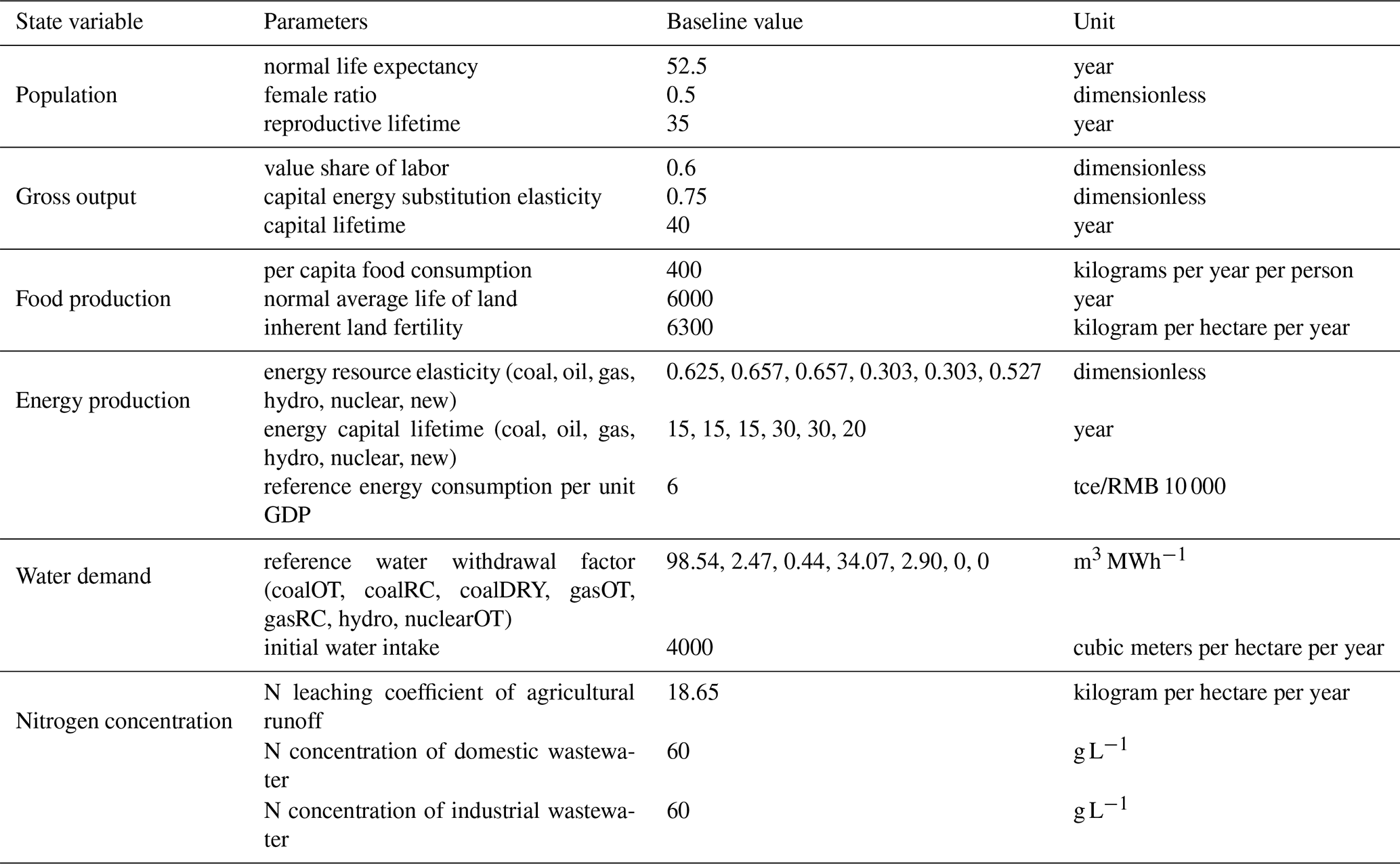
Note that the values of N concentrations for domestic and industrial wastewater are from Henze and Comeau (2008), and the value of the N leaching coefficient of agricultural runoff is obtained from FAO (http://www.fao.org/3/w2598e/w2598e06.htm, last access: 16 May 2022). Energy resource elasticities are from ANEMI (Breach and Simonovic, 2021).
5.2 Model application
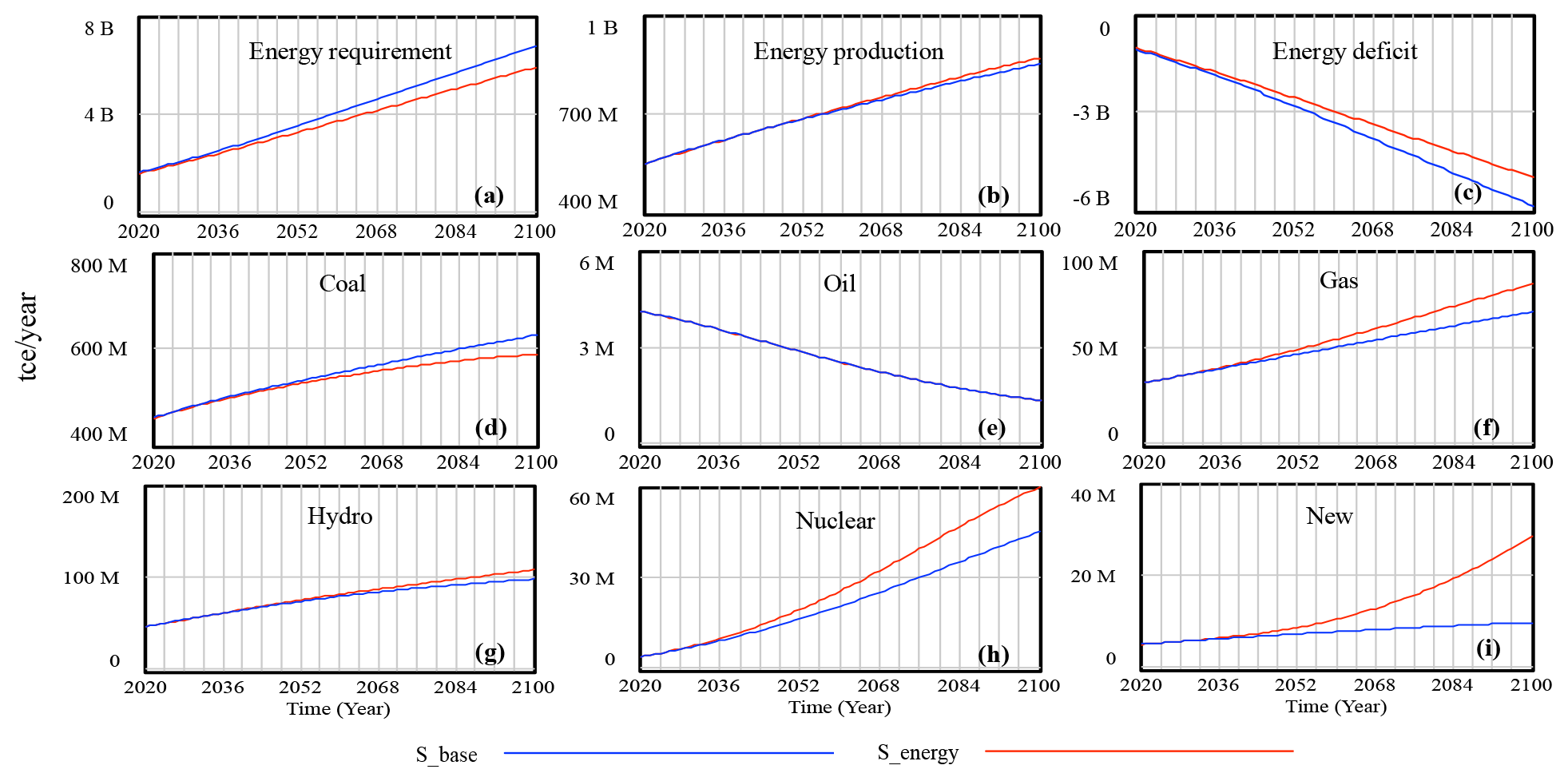
To test the capabilities of ANEMI_Yangtze, this section focuses on the applications of the model system for the baseline S_base scenario and S_energy scenario. The S_base scenario assumes that all parameters remain at their 2015 values during the simulation. The S_energy scenario assumes that the energy share of coal decreases linearly from around 60 % (the 2015 share) to 30 % and that the share of renewable energy (hydropower, nuclear, and new energy sources) increases from 15 % to 30 % by 2100. The simulation results are shown in Figs. 19–20.
As the share of gas and renewable energy sources increases in S_energy scenario, the demand for those energy sources grows, placing more pressure on their production. The energy production pressure effect acts as a positive factor on energy capital investment. Therefore, more money is poured into producing energy from gas and renewable sources. As more energy capital is mobilized for gas and renewable energy development, the improvement in energy technology advances correspondingly, leading to a decrease in energy consumption intensity per unit GDP, thus lowering the energy demand compared to the base run (Fig. 19a). Aside from this, the combined effects of growing energy capital investment and energy technology advancement lead to a substantial increase in effective production effort, resulting in increases in gas and renewable energy production (Fig. 19f–i). The production of coal is expected to decrease compared to the base run alongside a decrease in its energy share (Fig. 19d). Oil production remains at the base run level as its share remains the same value as in S_base scenario (Fig. 19e). The combined effect of the increase in gas and renewable energy production and the decrease in coal production result in a slight increase in the total production of energy compared to the base run result (Fig. 19b).
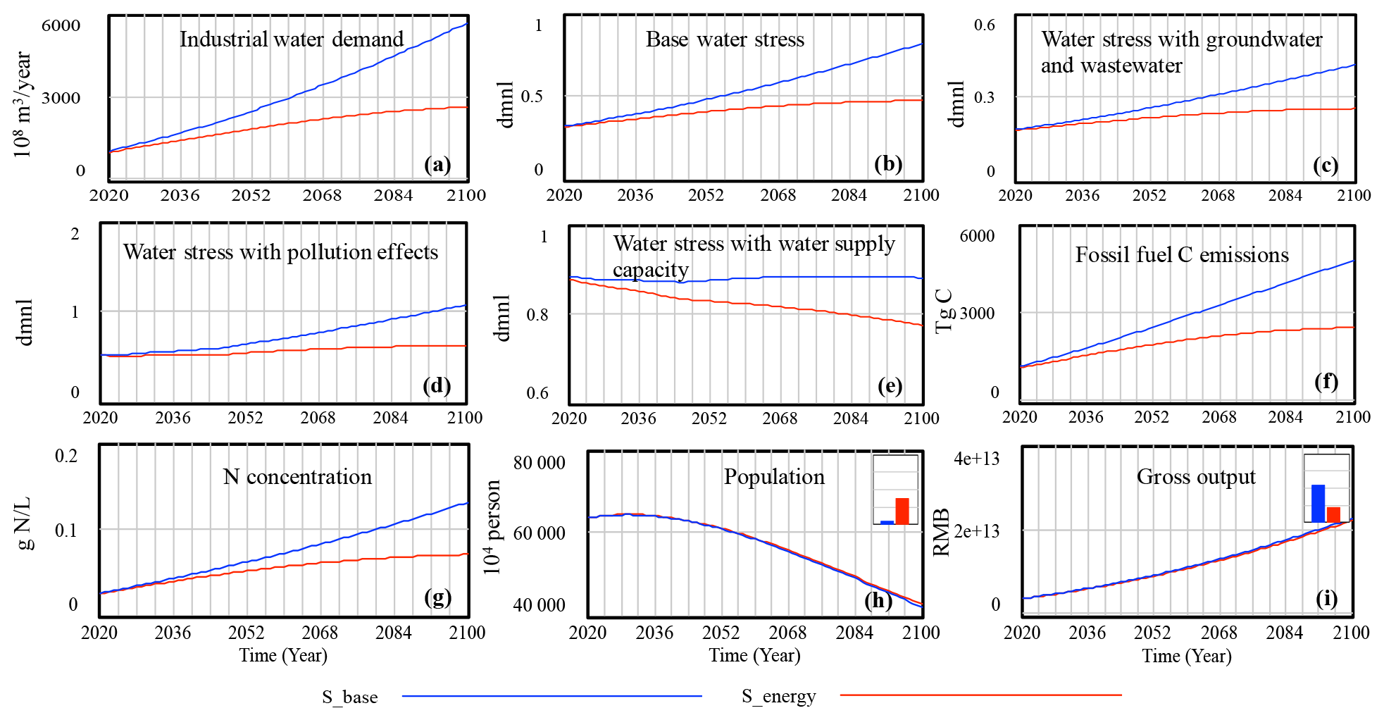
The changing patterns of energy consumption have significant impacts on water and carbon systems. In S_base run, coal-fired thermal power plants dominate the water demand in industrial sector (approaching 600 billion cubic meters), whereas in the S_energy scenario industrial water demand drops considerably below 300 billion cubic meters by the end of simulation as coal's share decreases from 60 % to 30 % (Fig. 20a). The industrial sector replaces the agricultural sector and becomes the biggest water consumer after 2030. Under all definitions, water stress declines substantially, with all values lying below the critical value of 1 (Fig. 20b–e). A decrease in industrial water demand and withdrawal also reduces industrial wastewater in accordance with this and lowers the level of nutrient concentration. The concentration level of nitrogen is shown in Fig. 20g; the results of phosphorus concentration, which share the same behavior as the nitrogen, are not shown in Fig. 20. By the end of the simulation, the carbon emissions fall from 4800 Tg in the S_base run to about 2500 Tg in the S_energy scenario as a result of cutting the coal consumption in half.
This changing energy consumption pattern also impacts population growth and economic development to some degree. A slight increase in population is observed under the S_energy scenario (Fig. 20h) when compared to the base run. This is due to the reduction in nitrogen and phosphorus concentration levels, which improve life expectancy through a single variable – lifetime multiplier from pollution. As for the economy, even though there is a slightly higher supply of labor force resulting from an increase in population, the Belt's gross output in the S_ energy scenario is a little bit lower than in the S_base output (Fig. 20i). This is due to the reduced energy requirement, as seen in Fig. 19a and discussed in Sect. 5.2. A decrease in energy requirements decreases the capital–energy aggregate, which then decreases the operating capital, leading to the decline in economic output. In this application, the effect of decreasing operating capital on economic output outpaces the effect of boosting the labor force on economic output.
To address the specific challenges facing the Yangtze Economic Belt's sustainable development, ANEMI_Yangtze, which consists of the population, economy, land, food, energy, water, carbon, nutrient, and fish sectors, was developed based on the feedback-based integrated global assessment model ANEMI3. This paper focuses on (i) the identification of the cross-sectoral interactions and feedbacks involved in shaping the Belt's system behavior over time; (ii) the identification of the feedbacks within each sector that drive the state variables in that sector; and (iii) the description of a new fish sector and modifications in the population, food, energy, and water sectors, including the underlying theoretical basis for model equations. The model was validated by comparing simulated results with historical data. Sensitivity analysis was conducted by varying the parameters with a high degree of uncertainty by −10 %–+10 % (mild-variation scenario) and −50 %–+50 % (extreme-variation scenario). Results demonstrate that the model is robust in modeling the behavior of the Belt system.
In Sect. 5, the impacts of shifting energy consumption patterns were investigated. As the Belt gradually shifts its energy consumption from coal to natural gas and renewable energy sources, the total energy production increases slightly. In contrast, the total aggregated energy requirement declines significantly due to the effects of energy technology advances. It is also found that the industrial water demand and the fossil fuel carbon emissions are greatly reduced, leading to a decrease in nutrient concentration levels and an increase in population. The Belt's gross output in the S_energy scenario is lower than the base output as the effect of decreasing operating capital, which is caused by a decrease in total aggregated energy requirement, outpaces the effect of boosting the labor force. These findings enhance our integrated understanding of the dynamic behavior of socio-economic development, natural resources depletion, and environmental impacts in the Belt. More in-depth model simulation analyses are needed to better understand the influences, responses, and feedbacks of the generic dynamic behavior of the Belt. The development of policy scenarios and the analyses of associated outcomes are presented in another paper (Jiang et al., 2021b).
This paper focuses on presenting the feedbacks that drive the Belt's dynamic system behavior based on the authors' current knowledge and understanding. It should, however, be kept in mind that some of the feedbacks might be missing due to the data necessary to describe these feedbacks not currently being available. For example, in China fish plays an important dietary role, and therefore there should be feedback connecting the fish yield and food production. Persistent pollution, a clear consequence of China's rapid economic development, should also be included. There are thus constant drivers to extend and improve the model framework as more data becomes available, as the state of the knowledge progresses, or as scientific questions become more complex.
The version of ANEMI_Yangtze described in this paper is archived on Zenodo (https://doi.org/10.5281/zenodo.4764138; Jiang et al., 2021a). The code can be opened using the Vensim software to view the model structure. A free Vensim PLE license can be obtained from https://vensim.com (last access: 8 June 2022), which can be used to view the stock and flow diagram that makes up the model structure. Due to the advanced features used in the ANEMI_Yangtze model, a Vensim DSS license is required to run the model.
Data are archived on Zenodo https://doi.org/10.5281/zenodo.4764138 (Jiang et al., 2021a). In the Vensim model, time series data enter into the model either as an Excel spreadsheet (by using the GET XLS DATA() function) or as an auxiliary variable using the WITH LOOKUP(Time) function. In ANEMI_Yangtze, we treat the time series data as auxiliary variables. In other words, the external time series data are “built in” the Vensim model, and thus anyone can run the Vensim model file .mdl without accessing the external .xls data.
HJ developed the model under guidance from SPS and wrote the original draft. SPS and ZY acquired the funds and did the review and editing work.
The contact author has declared that neither they nor their co-authors have any competing interests.
Publisher's note: Copernicus Publications remains neutral with regard to jurisdictional claims in published maps and institutional affiliations.
The authors are thankful for the financial support provided to Slobodan P. Simonovic by the Natural Sciences Research Council of Canada under the discovery grant program (grant no. RGPIN-2016-03693).
This research has been supported by the Belt and Road Special Foundation of the State Key Laboratory of Hydrology-Water Resources and Hydraulic Engineering (grant no. 2020490111), the Fundamental Research Funds for the Central Universities (grant no. B200202035), the Natural Sciences Research Council of Canada (grant no. RGPIN-2016-03693), the National Natural Science Foundation of China (grant nos. 51539003, 41761134090, and 51709074), and the Special Fund of State Key Laboratory of Hydrology-Water Resources and Hydraulic Engineering (grant nos. 20195025612, 20195018812, and 520004412).
This paper was edited by Daniel Huppmann and reviewed by Evan Davies and two anonymous referees.
Akhtar, M. K., Wibe, J., Simonovic, S. P., and MacGee, J.: Integrated assessment model of society-biosphere-climate-economy-energy system, Environ. Modell. Softw., 49, 1–21, https://doi.org/10.1016/j.envsoft.2013.07.006, 2013.
Akhtar, M. K., Simonovic, S. P., Wibe, J., and MacGee, J.: Future realities of climate change impacts: An integrated assessment study of Canada, Int. J. Global Warm., 17, 59–88, https://doi.org/10.1504/IJGW.2019.10017598, 2019.
Allen, C., Metternicht, G., and Wiedmann, T.: National pathways to the Sustainable Development Goals (SDGs): A comparative review of scenario modelling tools, Environ. Sci. Policy, 66, 199–207, https://doi.org/10.1016/j.envsci.2016.09.008, 2016.
Bauer, N., Baumstark, L., and Leimbach, M.: The REMIND-R model: The role of renewables in the low-carbon transformation – first-best vs. second-best worlds, Clim. Change, 114, 145–168, https://doi.org/10.1007/s10584-011-0129-2, 2012.
Bazilian, M., Rogner, H., Howells, M., Hermann, S., Arent, D., Gielen, D., Steduto, P., Mueller, A., Komor, P., Tol, R. S., and Yumkella, K. K.: Considering the energy, water and food nexus: Towards an integrated modelling approach, Energ. Policy, 39, 7896–7906, https://doi.org/10.1016/j.enpol.2011.09.039, 2011.
Breach, P.: Water Supply Capacity Development in the Context of Global Change, Electronic Thesis and Dissertation Repository, 6930, https://ir.lib.uwo.ca/etd/6930 (last access: 8 June 2022), 2020.
Breach, P. A. and Simonovic, S. P.: ANEMI: A tool for global change analysis, Plos One, 16, 0251489, https://doi.org/10.1371/journal.pone.0251489, 2021.
Calvin, K. and Bond-Lamberty, B.: Integrated human-earth system modeling – state of the science and future directions, Environ. Res. Lett., 13, 063006, https://doi.org/10.1088/1748-9326/aac642, 2018.
Calvin, K., Patel, P., Clarke, L., Asrar, G., Bond-Lamberty, B., Cui, R. Y., Di Vittorio, A., Dorheim, K., Edmonds, J., Hartin, C., Hejazi, M., Horowitz, R., Iyer, G., Kyle, P., Kim, S., Link, R., McJeon, H., Smith, S. J., Snyder, A., Waldhoff, S., and Wise, M.: GCAM v5.1: representing the linkages between energy, water, land, climate, and economic systems, Geosci. Model Dev., 12, 677–698, https://doi.org/10.5194/gmd-12-677-2019, 2019.
Cao, L., Zhang, Y., and Shi, Y.: Climate change effect on hydrological processes over the Yangtze River basin, Quaternary Int., 244, 202–210, https://doi.org/10.1016/j.quaint.2011.01.004, 2011.
Chen, D., Xiong, F., Wang, K., and Chang, Y.: Status of research on Yangtze fish biology and fisheries, Environ. Biol. Fish., 85, 337–357, https://doi.org/10.1007/s10641-009-9517-0, 2009.
Clark, W. A. V., Yi, D., and Zhang, X.: Do house prices affect fertility behavior in China? An empirical examination, Int. Regional Sci. Rev., 43, 423–449, https://doi.org/10.1177/0160017620922885, 2020.
Davies, E. G. R. and Simonovic, S. P.: ANEMI: A new model for integrated assessment of global change, Int. Environ. Rev., 11, 127–161, https://doi.org/10.1504/IER.2010.037903, 2010.
Davies, E. G. R. and Simonovic, S. P.: Global water resources modeling with an integrated model of the social-economic-environmental system, Adv. Water Resour., 34, 684–700, https://doi.org/10.1016/j.advwatres.2011.02.010, 2011.
Department of Energy at National Bureau of Statistics (DENBS): China Energy Statistical Yearbook in 2015, China Statistics Press, Beijing, 2016 (in Chinese).
Dermody, B. J., Sivapalan, M., Stehfest, E., van Vuuren, D. P., Wassen, M. J., Bierkens, M. F. P., and Dekker, S. C.: A framework for modelling the complexities of food and water security under globalisation, Earth Syst. Dynam., 9, 103–118, https://doi.org/10.5194/esd-9-103-2018, 2018.
Dettling, L. J. and Kearney, M. S.: House prices and birth rates: The impact of the real estate market on the decision to have a baby, J. Public Econ., 1, 82–100, https://doi.org/10.1016/j.jpubeco.2013.09.009, 2014.
Dinar, A., Tieu, A., and Huynh, H.: Water scarcity impacts on global food production, Glob. Food Secur., 23, 212–226, https://doi.org/10.1016/j.gfs.2019.07.007, 2019.
D'Odorico, P., Davis, K. F., Rosa, L., Carr, J. A., Chiarelli, D., Dell’Angelo, J., Gephart, J., MacDonald, G. K., Seekell, D. A., Suweis, S., and Rulli, M. C.: The global food©/energy©/water nexus, Rev. Geophys., 56, 456–531, https://doi.org/10.1029/2017RG000591, 2018.
European Commission: Energy in Europe, European energy to 2020: A scenario approach, Belgium, Directorate general for energy, 1996.
Fang, Y., Zhang, W., Cao, J., and Zhu, L.: Analysis on the current situation and development trend of energy resources in China, Conservation and Utilization of Mineral Resources, 4, 34–42, 2018 (in Chinese).
Fiddaman, T. S.: Feedback complexity in integrated climate-economy models, PhD thesis, Department of Operations Management and System Dynamics, Massachusetts Institute of Technology, Cambridge, Massachusetts, 360 pp., 1997.
Fisher-Vanden, K. and Weyant, J.: The evolution of integrated assessment: Developing the next generation of use-inspired integrated assessment tools, Annu. Review Resour. Econ., 12, 471–487, https://doi.org/10.1146/annurev-resource-110119-030314, 2020.
Forrester, J. W.: Industrial dynamics, Cambridge The M.I.T. press, Cambridge, MA, https://ocul-uwo.primo.exlibrisgroup.com/permalink/01OCUL_UWO/r0c2m8/alma991020555339705163 (last access: 8 June 2022), 1961.
Fu, B.: Promoting geography for sustainability, Geogr. Sustain., 1, 1–7, https://doi.org/10.1016/j.geosus.2020.02.003, 2020.
Giorgi, F., Im, E. S., Coppola, E., Diffenbaugh, N. S., Gao, X. J., Mariotti, L., and Shi, Y.: Higher hydroclimatic intensity with global warming, J. Climate, 24, 5309–5324, https://doi.org/10.1175/2011JCLI3979.1, 2011.
Gilbert, D. J., McKenzie, J. R., Davies, N. M., and Field, K. D.: Assessment of the SNA 1 stocks for the 1999–2000 fishing year, New Zealand Fisheries Assessment Report, 38, 52, 2000.
Goudriaan, J. and Ketner, P.: A simulation study for the global carbon cycle, including man's impact on the biosphere, Clim. Change, 6, 167–192, 1984.
Gu, H., Yu, Z., Wang, G., Wang, J., Ju, Q., Yang, C., and Fan, C.: Impact of climate change on hydrological extremes in the Yangtze river basin, China, Stoch. Env. Res. Risk A., 29, 693–707, https://doi.org/10.1007/s00477-014-0957-5, 2015.
Henze, M. and Comeau, Y.: Wastewater Characterization, in: Biological Wastewater Treatment: Principles Modelling and Design, IWA Publishing, London, UK, 33–52, 2008.
Hertwich, E. G., Gibon, T., Bouman, E. A., Arvesen, A., Suh, S., Heath, G. A., Bergesen, J. D., Ramirez, A., Vega, M. I., and Shi, L.: Integrated life-cycle assessment of electricity-supply scenarios confirms global environmental benefit of low-carbon technologies, P. Natl. Acad. Sci. USA, 112, 6277–6282, https://doi.org/10.1073/pnas.1312753111, 2015.
Holman, I. P., Rounsevell, M. D. A., Cojacaru, G., Shackley, S., McLachlan, C., Audsley, E., Berry, P. M., Fontaine, C., Harrison, P. A., Henriques, C., and Mokrech, M.: The concepts and development of a participatory regional integrated assessment tool, Clim. Change, 90, 5–30, https://doi.org/10.1007/s10584-008-9453-6, 2008.
Hopwood, B., Mellor, M., and O'Brien, G.: Sustainable development: Mapping different approaches, Sustain. Dev., 13, 38–52, https://doi.org/10.1002/sd.244, 2005.
Hui, E., Xian, Z., and Jiang, H.: Housing price, elderly dependency and fertility behaviour, Habitat Int., 36, 304–311, https://doi.org/10.1016/j.habitatint.2011.10.006, 2012.
Jeon, S., Roh, M., Oh, J., and Kim, S.: Development of an integrated assessment model at provincial level: GCAM-Korea, Energies, 13, 2565, https://doi.org/10.3390/en13102565, 2020.
Jia, B., Zhou, J., Zhang, Y., Tian, M., He, Z., and Ding, X.: System dynamics model for the coevolution of coupled water supply – power generation – environment systems: Upper Yangtze river Basin, China, J. Hydrol., 593, 125892, https://doi.org/10.1016/j.jhydrol.2020.125892, 2021.
Jiang, H. and Simonovic, S. P.: ANEMI_Yangtze – A regional integrated assessment model for the Yangtze Economic Belt in China, Water Resources Research Report no. 110, Facility for Intelligent Decision Support, Department of Civil and Environmental Engineering, London, Ontario, Canada, 75 pp., ISBN 978-0-7714-3155-5, 2021.
Jiang, H., Simonovic, S. P., Yu, Z., and Wang, W. G.: System dynamics simulation model for flood management of the three gorges reservoir, J. Water Res. Plan. Man., 146, 05020009, https://doi.org/10.1061/(ASCE)WR.1943-5452.0001216, 2020.
Jiang, H., Simonovic, S. P., and Yu, Z.: ANEMI_Yangtze (v1.0), Zenodo [code and data set], https://doi.org/10.5281/zenodo.4764138, 2021a.
Jiang, H., Simonovic, S. P., Yu, Z., and Wang, W. G.: What are the main challenges facing the sustainable development of China's Yangtze Economic Belt in the future? An integrated view, Environ. Res. Commun., 3, 115005, https://doi.org/10.1088/2515-7620/ac35bd, 2021b.
Ju, H., Liu, Q., Li, Y., Long, X., Liu, Z., and Lin, E.: Multi-stakeholder efforts to adapt to climate change in China's agricultural sector, Sustainability, 12, 8076, https://doi.org/10.3390/su12198076, 2020.
Klein, J. T.: Transdisciplinarity: Joint problem solving among science, technology, and society: An effective way for managing complexity, Springer Science & Business Media, Basel, Switzerland, Boston, MA, ISBN 9783764362485, 2001.
Kong, L., Zheng, H., Rao, E., Xiao, Y., Ouyang, Z., and Li, C.: Evaluating indirect and direct effects of eco-restoration policy on soil conservation service in Yangtze River Basin, Sci. Total Environ., 631, 887–894, https://doi.org/10.1016/j.scitotenv.2018.03.117, 2018.
Kriegler, E., Bauer, N., Popp, A., Humpenöder, F., Leimbach, M., Strefler, J., Baumstark, L., Bodirsky, B. L., Hilaire, J., Klein, D., Mouratiadou, I., Weindl, I., Bertram, C., Dietrich, J.-P., Luderer, G., Pehl, M., Pietzcker, R., Piontek, F., Lotze-Campen, H., Biewald, A., Bonsch, M., Giannousakis, A., Kreidenweis, U., Müller, C., Rolinski, S., Schultes, A., Schwanitz, J., Stevanovic, M., Calvin, K., Emmerling, J., Fujimori, S., and Edenhofer, O.: Fossil-fueled development (SSP5): An energy and resource intensive scenario for the 21st century, Global Environ. Chang., 42, 297–315, https://doi.org/10.1016/j.gloenvcha.2016.05.015, 2017.
Lee, E. S.: A Theory of Migration, Demography, 3, 47–57, 1966.
Lei, G., Fu, C., Zhang, L., Zeng, X., and Wang, W.: The changes in population floating and their influencing factors in China based on the sixth census, Northwest Population Journal, 34, 1–8, https://doi.org/10.15884/j.cnki.issn.1007-0672.2013.05.017, 2013 (in Chinese).
Li, Y., Acharya, K., and Yu, Z.: Modeling impacts of Yangtze River water transfer on water ages in Lake Taihu, China, Ecol. Eng., 37, 325–334, https://doi.org/10.1016/j.ecoleng.2010.11.024, 2011.
Li, Z., He, Y., Pu, T., Jia, W., He, X., Pang, H., Zhang, N., Liu, Q., Wang, Sh., Zhu, G., Wang, Sh., Chang, L., Du, J., and Xin, H.: Changes of climate, glaciers and runoff in China's monsoonal temperate glacier region during the last several decades, Quaternary Int., 218, 13–28, https://doi.org/10.1016/j.quaint.2009.05.010, 2010.
Liu, J. G., Dietz, T., Carpenter, S. R., Alberti, M., Folke, C., Moran, E., Pell, A. N., Deadman, P., Kratz, T., Lubchenco, J., Ostrom, E., Ouyang, Z., Provencher, W., Redman, C. L., Schneider, S. H., and Taylor, W. W.: Complexity of coupled human and natural systems, Science, 317, 1513–1516, https://doi.org/10.1126/science.1144004, 2007.
Liu, L. and Ding, Y.: Hydraulic resources and hydropower planning in the Yangtze River Basin, Yangtze River, 44, 69–71, 2013 (in Chinese).
Loulou, R.: ETSAP-TIAM: The TIMES integrated assessment model. Part II: Mathematical formulation, Comput. Manag. Sci., 5, 41–66, https://doi.org/10.1007/s10287-007-0045-0, 2007.
Ma, L. and Yu, Z.: Influencing factors of Chinese average life expectancy, Economic Research Guide, 01, 161–162, 2009.
Mackenzie, F. T., Ver, L. M., Sabine, C., and Lane, M.: C, N, P, S global biogeochemical cycles and modeling of global change, in: Interactions of C, N, P and S Biogeochemical Cycles and Global Change, edited by: Wollast, R., Mackenzie, F. T., and Chou, L., North Atlantic Treaty Organization Scientific Affairs Division, NATO advanced research workshop on interactions of C, N, P, and S biogeochemical cycles, Springer Verlag, New York, 1–61, ISBN 0387531262, 1991.
Matsuoka, Y., Kainuma, M., and Morita, T.: Scenario analysis of global warming using the Asian-Pacific integrated model (AIM), Energ. Policy, 23, 357–371, https://doi.org/10.1016/0301-4215(95)90160-9, 1995.
Meadows, D. L.: The Dynamics of growth in a finite world, Wright-Allen Press, Inc. Cambrigde, Massachusetts, ISBN 0960029443, 1974.
Messner, S. and Schrattenholzer, L.: MESSAGE-MACRO: linking an energy supply model with a macroeconomic module and solving it iteratively, Energy, 25, 267–282, https://doi.org/10.1016/S0360-5442(99)00063-8, 2000.
Messner, S. and Strubegger, M.: User's Guide for MESSAGE III, Working Paper WP-95-069, International Institute for Applied Systems Analysis (IIASA), Laxenburg, Austria, 164 pp., 1995.
MIIT: Innovation-driven industrial transformation and upgrading plan for the Yangtze River Economic Belt, Ministry of Industry and Information Technology of the People's Republic of China, 2016.
National Development and Reform Commission (NDRC): Development and planning outline of the Yangtze River Economic Belt officially released, http://www.sc.gov.cn/10462/10758/10760/10765/2016/9/20/10396398.shtml (last access: 8 June 2022), 2016.
Niva, V., Cai, J., Taka, M., Kummu, M., and Varis, O.: China's sustainable water-energy-food nexus by 2030: Impacts of urbanization on sectoral water demand, J. Clean. Prod., 251, 119755, https://doi.org/10.1016/j.jclepro.2019.119755, 2020.
Nordhaus, W. D. and Boyer, J.: Warming the world: Economic models of global warming, The MIT Press, Cambridge, Massachusetts, USA, ISBN 0-262-14071-3, 2000.
Pautrel, X.: Pollution and life expectancy: How environmental policy can promote growth, Ecol. Econ., 68, 1040–1051, https://doi.org/10.1016/j.ecolecon.2008.07.011, 2009.
Pedercini, M., Arquitt, S., Collste, D., and Herren, H.: Harvesting synergy from sustainable development goal interactions, P. Natl. Acad. Sci. USA, 46, 23021–23028, https://doi.org/10.1073/pnas.1817276116, 2019.
Qin, B. Q., Wang, X. D., Tang, X. M., Feng, S., and Zhang, Y. L.: Drinking water crisis caused by eutrophication and cyanobacterial bloom in Lake Taihu: cause and measurement, Adv. Earth Sci., 22, 896–906, https://doi.org/10.3321/j.issn:1001-8166.2007.09.003, 2007 (in Chinese).
Qu, W., Barney, G., Symalla, D., and Martin, L.: Threshold 21: National sustainable development model, Integrated Global Models of Sustainable Development, 2, 78–87, 1995.
Qu, W., Shi, W., Zhang, J., and Liu, T.: T21 China 2050: A tool for national sustainable development planning, Geogr. Sust., 1, 33–46, https://doi.org/10.1016/j.geosus.2020.03.004, 2020.
Shen, J.: Increasing internal migration in China from 1985 to 2005: Institutional versus economic drivers, Habitat Int., 39, 1–7, https://doi.org/10.1016/j.habitatint.2012.10.004, 2013.
Shi, W., Ou, Y., Smith, S. J., Ledna, C. M., Nolte, C. G., and Loughlin, D. H.: Projecting state-level air pollutant emissions using an integrated assessment model: GCAM-USA, Appl. Energ., 208, 511–521, https://doi.org/10.1016/j.apenergy.2017.09.122, 2017.
Shiklomanov, I. A.: Appraisal and assessment of world water resources, Water Int., 25, 11–32, https://doi.org/10.1080/02508060008686794, 2000.
Simonovic, S. P.: Global water dynamics: Issues for the 21st century, J. Water Sci. Technol., 45, 53–64, https://doi.org/10.2166/wst.2002.0143, 2002a.
Simonovic, S. P.: World water dynamics: Global modeling of water resources, J. Environ. Manage., 66, 249–267, https://doi.org/10.1006/jema.2002.0585, 2002b.
Simonovic, S. P.: Managing water resources: Methods and tools for a systems approach, Earthscan James & James, London, ISBN 9231040782, 2009.
Song, Q.: Study on the wind resource distribution and wind power planning in China, North China Electric Power University, 2013 (in Chinese).
State Grid Energy Research Institution (SGERI), and China Nuclear Power Development Center (CNPD): Research on nuclear power development planning in China, China Atomic Energy Press, 2019 (in Chinese).
Stehfest, E., van Vuuren, D., Kram, T., and Bouwman, L.: Integrated assessment of global environmental change with IMAGE 3.0: Model description and policy applications, PBL Netherlands Environmental Assessment Agency, ISBN 978-94-91506-71-0, 2014.
Su, B., Huang, J., Zeng, X., Gao, C., and Jiang, T.: Impacts of climate change on streamflow in the upper Yangtze River basin, Clim. Change, 141, 533–546, https://doi.org/10.1007/s10584-016-1852-5, 2017.
Su, M.: Research on the coordinated development of energy in the Yangtze River Economic Zone, Macroeconomic Manage., 12, 37–41, 2019 (in Chinese).
Su, Y., Tesfazion, P., and Zhao, Z.: Where are the migrants from? Inter- vs. intra-provincial rural-urban migration in China, China Econ. Rev., 47, 142–155, https://doi.org/10.1016/j.chieco.2017.09.004, 2018.
Sullivan, P., Krey, V., and Riahi, K.: Impacts of considering electric sector variability and reliability in the MESSAGE model, Energy Strateg. Rev., 1, 157–163, https://doi.org/10.1016/j.esr.2013.01.001, 2013.
van Beek, L., Hajer, M., Pelzer, P., van Vuuren, D., and Cassen, C.: Anticipating futures through models: the rise of Integrated Assessment Modelling in the climate science-policy interface since 1970, Global Environ. Chang., 65, 102191, https://doi.org/10.1016/j.gloenvcha.2020.102191, 2020.
van Vuuren, D. P., Kok, M., Lucas, P. L., Prins, A. G., Alkemade, R., van den Berg, M., Bouwman, L., van der Esch, S., Jeuken, M., Kram, T., and Stehfest, E.: Pathways to achieve a set of ambitious global sustainability objectives by 2050: Explorations using the IMAGE integrated assessment model, Technol. Forecast. Soc., 98, 303–323, https://doi.org/10.1016/j.techfore.2015.03.005, 2015.
Wang, H.: Yangtze Yearbook, Changjiang Water Resources Commission of Ministry of Water Resources, 2015 (in Chinese).
Wang, H., Liu, L., Yang, F., and Ma, J.: System dynamics modeling of China's grain forecasting and policy simulation, J. Syst. Simul., 21, 3079–3083, 2009 (in Chinese).
Wang, Z., Nguyen, T., and Westerhoff, P.: Food-energy-water analysis at spatial scales for districts in the Yangtze river basin (China), Environ. Eng. Sci., 36, 789–797, https://doi.org/10.1089/ees.2018.0456, 2019.
Xie, H. and Wang, B.: An empirical analysis of the impact of agricultural product price fluctuations on China's grain yield, Sustainability, 9, 906, https://doi.org/10.3390/su9060906, 2017.
Xu, X., Yang, G., Tan, Y., Liu, J., and Hu, H.: Ecosystem services trade-offs and determinants in China's Yangtze River Economic Belt from 2000 to 2015, Sci. Total Environ., 634, 1601–1614, https://doi.org/10.1016/j.scitotenv.2018.04.046, 2018.
Yangtze River Water Resources Commission (YRWRC): Water resources bulletin of the Yangtze river basin and the southwest rivers in China 2015, Yangtze River Press, Wuhan, 2016 (in Chinese).
Yao, G., Gao, Z., and Li, X.: Evaluation of coal resources bearing capacity in China, China Mining Magazine, 29, 1–7, 2020 (in Chinese).
Ye, L., Wei, X., Li, Z., Yang, P., Wu, W., Yang, G., Fu, Y., Zou, J., Chen, Z., Ranst, E. V., and Tang, H.: Climate change impact on China food security in 2050, Agron. Sustain. Dev., 33, 363–374, https://doi.org/10.1007/s13593-012-0102-0, 2013.
Yi, B. L., Yu, Z. T., and Liang, Z. S.: Gezhouba Water Control Project and four famous fishes in the Yangtze River, Hubei Science and Technology Press, Wuhan, edited by: Huang, X., ISBN 7-5352-0334-2/s.36, 1988, (in Chinese with English abstract).
Yu, S., Yarlagadda, B., Siegel, J. E., Zhou, S., and Kim, S.: The role of nuclear in China's energy future: Insights from integrated assessment, Energ. Policy, 139, 111344, https://doi.org/10.1016/j.enpol.2020.111344, 2020.
Yu, Z., Gu, H., Wang, J., Xia, J., and Lu, B.: Effect of projected climate change on the hydrological regime of the Yangtze River Basin, China, Stoch. Env. Res. Risk A., 32, 1–16, https://doi.org/10.1007/s00477-017-1391-2, 2018.
Zeng, Y. and Hesketh, T.: The effects of China's universal two-child policy, The Lancet, 388, 1930–1938, https://doi.org/10.1016/S0140-6736(16)31405-2, 2016.
Zhang, C., Zhong, L., Fu, X., Wang, J., and Wu, Z.: Revealing water stress by the thermal power industry in China based on a high spatial resolution water withdrawal and consumption inventory, Environ. Sci. Technol., 50, 1642–1652, https://doi.org/10.1021/acs.est.5b05374, 2016.
Zhang, H., Li, J. Y., Wu, J. M., Wang, C. Y., Du, H., Wei, Q. W., and Kang, M.: Ecological effects of the first dam on Yangtze main stream and future conservation recommendations: A review of the past 60 years, Appl. Ecol. Env. Res., 15, 2081–2097, https://doi.org/10.15666/aeer/1504_20812097, 2017.
Zhang, H., Kang, M., Shen, L., Wu, J., Li, J., Du, H., Wang, C., Yang, H., Zhou, Q., Liu, Z., Gorfine, H., and Wei, Q.: Rapid change in Yangtze fisheries and its implications for global freshwater ecosystem management, Fish Fish., 21, 601–620, https://doi.org/10.1111/faf.12449, 2020.
Zhao, F. and Fan, Z.: The inhibitory effect of high housing prices on population inflows in the megacities: Based on the empirical evidence from the four cities of Beijing, Shanghai, Guangzhou and Shenzhen, Urban Studies, 26, 41–48, 2019 (in Chinese).
Zhu, R., Ma, S., Yang, Z., and Zhou, C.: Atlas of solar energy resources by province in China, China Meteorological Administration, Beijing, 2006 (in Chinese).
- Abstract
- Introduction
- Yangtze Economic Belt: system description
- ANEMI_Yangtze: background and theoretical basis
- ANEMI_Yangtze: model development
- Model validation and application
- Conclusion and discussion
- Code availability
- Data availability
- Author contributions
- Competing interests
- Disclaimer
- Acknowledgements
- Financial support
- Review statement
- References