the Creative Commons Attribution 4.0 License.
the Creative Commons Attribution 4.0 License.
 | 06 Jan 2022
WOMBAT v1.0: a fully Bayesian global flux-inversion framework
Michael Bertolacci
Jenny Fisher
Ann Stavert
Matthew Rigby
Yi Cao
Noel Cressie
WOMBAT (the WOllongong Methodology for Bayesian Assimilation of Trace-gases) is a fully Bayesian hierarchical statistical framework for flux inversion of trace gases from flask, in situ, and remotely sensed data. WOMBAT extends the conventional Bayesian synthesis framework through the consideration of a correlated error term, the capacity for online bias correction, and the provision of uncertainty quantification on all unknowns that appear in the Bayesian statistical model. We show, in an observing system simulation experiment (OSSE), that these extensions are crucial when the data are indeed biased and have errors that are spatio-temporally correlated. Using the GEOS-Chem atmospheric transport model, we show that WOMBAT is able to obtain posterior means and variances on non-fossil-fuel CO2 fluxes from Orbiting Carbon Observatory-2 (OCO-2) data that are comparable to those from the Model Intercomparison Project (MIP) reported in Crowell et al. (2019). We also find that WOMBAT's predictions of out-of-sample retrievals obtained from the Total Column Carbon Observing Network (TCCON) are, for the most part, more accurate than those made by the MIP participants.
Please read the corrigendum first before continuing.
-
Notice on corrigendum
The requested paper has a corresponding corrigendum published. Please read the corrigendum first before downloading the article.
-
Article
(4966 KB)
- Corrigendum
-
Supplement
(299 KB)
-
The requested paper has a corresponding corrigendum published. Please read the corrigendum first before downloading the article.
- Article
(4966 KB) - Full-text XML
- Corrigendum
-
Supplement
(299 KB) - BibTeX
- EndNote


Atmospheric carbon dioxide (CO2) is a leading driver of global warming (e.g. Peters et al., 2013). If left unchecked, the rise in global temperatures will have a substantial negative impact on society and the environment (e.g. Edenhofer et al., 2014). As part of the worldwide effort to limit these impacts, the 2015 Paris Agreement under the United Nations Framework Convention on Climate Change, COP 21, called for a global stocktake of the sources and sinks of CO2 and other greenhouse gases, with the first evaluation planned for 2023 (UNFCCC, 2015). The rate at which CO2 is emitted (from sources) or absorbed (at sinks) per unit space and time is known as the CO2 flux, which itself varies spatio-temporally in a substantial manner. Despite the fact that it is human emissions that are driving the rise in atmospheric CO2 concentrations, the most uncertain aspects of quantifying CO2 fluxes at Earth's surface centre around natural processes. For example, while we know that the land and oceans absorb more than half of the CO2 emitted by human activities (e.g. Dlugokencky and Tans, 2020), the geographical and temporal patterns of these sinks remain unclear (e.g. Crowell et al., 2019).
Monitoring the progression of CO2 in our atmosphere is thus of utmost importance, and billions of dollars have been spent over the last few decades on research, development, and deployment of instruments for measuring CO2 mole fraction (defined here as the proportion of CO2 molecules in a given parcel of dry air) across the globe (e.g. Burrows et al., 1995; Kuze et al., 2009; Wunch et al., 2011a; Masarie et al., 2014; Eldering et al., 2017, 2019). However, CO2 mole fraction is only indirectly related to the key quantity of interest, namely the geographic distribution of the CO2 fluxes over time, which cannot be observed directly on regional scales. Identifying these sources and sinks spatially and temporally is an ill-posed inverse problem, often called a trace-gas flux-inversion problem, whose solution requires the use of both an atmospheric transport model and a spatio-temporal model for the fluxes (e.g. Enting, 2002). In this paper, we present version 1.0 of a global flux-inversion system for the solution of this problem, which we call the WOllongong Methodology for Bayesian Assimilation of Trace-gases (WOMBAT).
A global trace-gas flux-inversion system is designed to infer fluxes from observational data, which are generally available either as point-referenced (flask or in situ) measurements or column-averaged remote sensing retrievals. The underlying model in an inversion system is usually a state-space model, where the fluxes, or a reduced representation thereof, are the latent states that need to be inferred from data via the use of an atmospheric chemical transport model (CTM). Computationally, flux estimation is done within a standard optimisation framework (e.g. Chevallier et al., 2005; Baker et al., 2006), either via full Bayesian synthesis (e.g. Enting, 2002, chap. 3; Mukherjee et al., 2011; Schuh et al., 2019) or via ensemble Kalman filtering (e.g. Peters et al., 2005; Feng et al., 2009). Inversion systems rely, to various extents, on realistic bottom-up estimates of fluxes for the elicitation of an informative prior distribution, an accurate CTM that provides the link between the fluxes and the observed mole fraction, high-quality unbiased measurements, and reliable uncertainty measures on each model component.
The complexity of all modelled processes, from fluxes right up to satellite retrieval errors, inevitably leads to model misspecification (e.g. Engelen et al., 2002). The main causes of misspecification are (i) flux-process dimension-reduction error (e.g. Kaminski et al., 2001), which is a consequence of using a spatio-temporal model for the flux field that is low dimensional and inflexible; (ii) an inaccurate prior flux mean, variance, and covariance (e.g. Philip et al., 2019); (iii) transport model errors (e.g. Houweling et al., 2010; Basu et al., 2018; Schuh et al., 2019) arising from the underlying assumed physics, meteorology, and discretisation schemes used (e.g. Lauvaux et al., 2019; McNorton et al., 2020); (iv) retrieval biases (e.g. O'Dell et al., 2018) and incorrect associated measurement error statistics (e.g. Worden et al., 2017); and (v) measurement error spatio-temporal correlations that are not fully accounted for (e.g. Chevallier, 2007; Ciais et al., 2010). Two other causes of model misspecification worth noting are an incorrectly specified initial global mole-fraction field and flux components assumed known in the inversion (i.e. assumed degenerate at their prior mean), such as anthropogenic emissions (e.g. Feng et al., 2019). The latter can be seen as a special case of (i) above, while the effect of the former can generally be minimised by using a realistic initial condition (e.g. Basu et al., 2013) and incorporating a burn-in (or spin-up) period in which early flux estimates are discarded.
In Sect. 2, we present the underlying statistical framework of WOMBAT, which addresses the implications of model misspecification in four ways: first, by using prior distributions to encode uncertainty over prior beliefs on the fluxes (sometimes referred to as hyperprior distributions; see, e.g. Ganesan et al., 2014; Zammit-Mangion et al., 2016), second, by adding a spatio-temporally correlated component of variability to the mole-fraction data model to address some of this (typically unmodelled) correlated model–data discrepancy (Brynjarsdóttir and O'Hagan, 2014), third, by explicitly modelling biases in the mole-fraction data model (generalising the approach of Basu et al., 2013), and fourth, by propagating uncertainty on all unknowns within a fully Bayesian statistical framework wherein inference is made using Markov chain Monte Carlo (MCMC). We note that while the benefits of MCMC are becoming increasingly apparent in regional trace-gas inversions (e.g. Mukherjee et al., 2011; Ganesan et al., 2014; Miller et al., 2014; Zammit-Mangion et al., 2016), its use is still the exception rather than the rule in global trace-gas inversions. The use of a spatio-temporally correlated component of variability leads to computational challenges, which are addressed in Sect. 3. We also note that our MCMC framework allows the uncertainties over the fluxes to be affected by uncertainties over all unknown parameters in the model, and it is thus different from the Monte Carlo approach to estimating flux uncertainty used by, for example, Chevallier et al. (2007) and Liu et al. (2014).
The fully Bayesian nature of the model, coupled with the introduction of a correlated process in modelling the mole-fraction field, leads to computational challenges. Section 3 details how we deal with these by defining a specific type of stochastic process on the irregularly located spatio-temporal errors, one that leads to a sparse precision matrix (e.g. Vecchia, 1988; Datta et al., 2016). Details on how this facilitates the MCMC scheme we implement are deferred to Appendix A. Section 4 discusses the experimental setup used for running, validating, and implementing WOMBAT on the satellite data analysed in this article. In Sect. 5, we first conduct an observing system simulation experiment (OSSE) in which the true fluxes are assumed known. Results from the OSSE demonstrate WOMBAT's validity and also illustrate the importance of modelling biases and correlated error terms when these are indeed present in the data. We then use WOMBAT to perform flux inversion using the Orbiting Carbon Observatory-2 (OCO-2) Version 7 retrospective (V7r) dataset as used in the model intercomparison project (MIP) of Crowell et al. (2019). Our model fitting reveals that about 80 % of the total error variance associated with the OCO-2 data used for the MIP can be explained with a correlated model–data discrepancy term. WOMBAT accounts for this, which results in posterior distributions over the fluxes that, for the most part, corroborate the results from the ensemble inversions, both on a regional and on a global scale. In Sect. 5, we also show the utility of WOMBAT in carrying out online bias correction. Section 6 summarises the features of WOMBAT and discusses avenues for future work.
In this section we outline the spatio-temporal Bayesian hierarchical statistical model (e.g. Sect. 1.3, Wikle et al., 2019) that WOMBAT uses for global flux inversion. The model consists of four sub-models: (1) a flux process model, (2) a mole-fraction process model, (3) a mole-fraction data model, and (4) a parameter model.
2.1 The flux process model
Let denote the prior mean of the trace-gas surface flux at spatial location s∈𝕊2 and time t∈𝒯, where 𝕊2 is the surface of Earth and is some time interval of interest. The field could, for example, be treated as a linear regression (e.g. Michalak et al., 2004) or could be constructed using bottom-up estimates of biospheric and/or anthropogenic fluxes (e.g. Basu et al., 2013).
In the same vein as conventional Bayesian-synthesis frameworks (e.g. Enting, 2002), we model the true flux, , as plus a spatio-temporal field constructed through a sum of r spatio-temporal basis functions. These basis functions could be space–time step functions, as typically found in variational inversion systems (e.g. Chevallier et al., 2005), discretised flux “patterns” (e.g. Fan et al., 1998), or a general-purpose basis such as a Fourier basis (e.g. Crowell et al., 2019, Appendix A4).
We denote the set of pre-specified flux basis functions as . Our flux process model is a spatio-temporal stochastic process given by the following equation:
where the scaling factors are unknown, are assigned a multivariate probability distribution, and need to be inferred in the inversion framework. Since we assume that we let E(αj)=0 for For a given set of basis functions, the prior belief on the covariance structure of is fully determined by that on . When the flux is modelled on a space–time grid and space–time step functions are used as basis functions, a prior distribution on α that correlates the flux a priori in space and time is natural (Michalak et al., 2004; Chevallier et al., 2007; Basu et al., 2018). On the other hand, when using large spatial flux “patterns” that have temporally limited scope, it is generally reasonable to assume that any two of the αj corresponding to basis functions in different spatial regions are uncorrelated but that those associated with the same spatial region are temporally correlated.
Irrespective of the choice of basis functions, in WOMBAT one expresses prior judgement on α through the model , where Gau(μ,Σ) is a Gaussian probability density function of a random vector with mean μ and covariance matrix Σ. The covariance matrix Σα is parameterised through a parameter vector θα, which typically contains variances and spatio-temporal length scales in the covariances. Expert elicitation can be used to construct prior distributions on these parameters too; we describe possible prior distributions when discussing the parameter model in the Bayesian hierarchical model in Sect. 2.4.
The flux model of Eq. (1) may be improved by introducing a dimension-reduction error, also known as aggregation error, on the right-hand side. This error accounts for the fact that the structured basis functions typically span a small (function) space and that they therefore cannot reproduce fluxes perfectly. However, since we are unable to deconvolve dimension reduction error from other sources of error (e.g. transport model error) in our mole-fraction data, we model the spatio-temporal variability it introduces collectively with other sources of error (Sect. 2.2).
2.2 The mole-fraction process model
We denote the true mole-fraction process at horizontal location s, vertical height h, and time t as . We only model the mole fraction within our time interval of interest 𝒯, starting at time t0, and therefore we express the true mole-fraction field within 𝒯 as a function of the initial mole-fraction process at t0 and the exogenous flux-process inputs in 𝒯. Specifically, is defined for as the set of all time points in 𝒯 up to and including t. The field is related to the flux process through the following relationship:
for , where is the mole-fraction field at time t0, is the flux field evolving over the whole time period 𝒯t, and ℋ is an operator that solves the underlying chemical transport equations (that are approximately linear for long-lived species such as CO2; see, e.g. Enting, 2002, chap. 2). In practice, ℋ is not known perfectly, but we usually have at hand a reasonable approximation to it, , which is often referred to as the chemical transport model (CTM) or simply as the transport model. Similarly, we will usually have a reasonable approximation to , which we call . The use of instead of , and of instead of ℋ, leads to a residual term that will inevitably be spatio-temporally correlated (Enting, 2002, chap. 9). In particular,
for , where is the residual mole-fraction process arising from the use of an approximate initial mole-fraction field, imperfect meteorology inside the transport model, imperfect transport model parameters and physics, and potentially sub-grid-scale variation in the mole-fraction field when is a numerical model evaluated at a coarse resolution. It is difficult to place prior beliefs on the structure of , which we model as statistical error, but it is known that using the approximation introduces errors that could span hundreds of kilometres and several days (Lauvaux et al., 2019; McNorton et al., 2020). Transport model implementations tend to differ considerably in their vertical and inter-hemispheric mixing behaviour, and flux-inversion estimates are known to be particularly sensitive to transport model choice (Gurney et al., 2002; Schuh et al., 2019). Note that is also likely to depend on and that we ignore this dependence for model simplicity in what follows.
The assumed linear behaviour of the underlying dynamics for CO2 is important. First, it allows us to model the effect of the approximate initial mole-fraction field, , separately from that of the fluxes (e.g. Enting, 2002, chap. 10) so that Eq. (3) is of the following form:
for s∈𝕊2, , and t∈𝒯. Second, it allows us to express the mole-fraction field as a linear combination of the individual responses from the basis functions used to construct , as we now show. Substituting Eq. (1) into Eq. (4), we have the following equation:
for s∈𝕊2, , and t∈𝒯, where ; for , are basis functions in mole-fraction space, often termed “response functions” (e.g. Saeki et al., 2013); and is the residual term given in Eq. (3). We assume that , and thus can be seen as the prior expectation of the mole-fraction field at under and . That is, it is the mole-fraction field generated by running our CTM with the input fluxes set to the prior expected flux and with the mole-fraction field at t0 set to .
2.3 The mole-fraction data model
Fluxes cannot be observed directly at the spatial and temporal scales of interest. Flux inversion therefore proceeds by “constraining” the flux field using column-averaged retrievals or point-referenced measurements of mole fraction. We use Z2,i to denote the ith mole-fraction measurement or retrieval, where indexes the datum used in the inversion and m is the number of data used in the inversion.
Point-referenced (PR) measurements of mole fraction are generally made at or near Earth's surface using instruments on towers or in aircraft. The mole-fraction data model for these measurements is therefore given by
where Z2,i is the observed mole fraction at , and ϵi is mean-zero Gaussian measurement error, with a model for its variance parameter presented below in Sect. 2.4. Measurement errors associated with point-referenced instruments are generally small and (usually) not correlated in space and time. Despite this, such data are not immune to the effects of spatio-temporal correlations induced by the CTM in the process model, and they may even be more susceptible than column-averaged retrievals due to the combined effect of their usual proximity to the surface and the discretisations employed when simulating approximate transport (Rayner and O'Brien, 2001; Basu et al., 2018).
Column-averaged (CA) retrievals, such as XCO2 (where “X” refers to the column-averaged nature of the retrievals) from the OCO-2 satellite or the Total Column Carbon Observing Network (TCCON) sites, are noisier than PR measurements, although TCCON is less noisy. In particular, since the raw spectral information collected for the retrieval is affected by environmental factors such as aerosols (O'Dell et al., 2012), the errors can contain biases and exhibit spatio-temporal correlations. These biases can also be instrument-mode dependent (e.g. land glint, LG, vs. land nadir, LN, retrievals for OCO-2; see Sect. 4.4.1). The vertical averaging operation also involves an averaging kernel and an a priori bias correction, which are both specific to the retrieval and which arise from the algorithm used for the retrieval. In general, this relationship can be expressed as follows:
where (si,ti) is the space–time location of the retrieval, is the assumed (but necessarily approximate) observation operator of the ith retrieval that column-averages the mole fraction field via an averaging kernel, bi is bias, is mean-zero spatio-temporally correlated random error, and ϵi is mean-zero uncorrelated random error. The bias and error terms arise from the use of an approximate observation operator. Surface-based or remotely sensed CA retrievals are sometimes provided as “bias-corrected retrievals”. In this case, the data model for these retrievals is identical to Eq. (7), but with the bias component omitted.
Substituting Eq. (5) into Eqs. (6) and (7) we see that, in general, we have
where, for a PR measurement, , , for , and while for a CA retrieval, , , for ; and . Bias-corrected retrievals are given by Eq. (8) but with the bias component bi omitted. Note that for identifiability reasons we have modelled all the possibly correlated error terms using one component, {ξi}.
Flux inversions can make use of both PR measurements and CA retrievals simultaneously, and hence it is convenient to provide a data model that encapsulates both types of measurements. It is also often the case that measurements from the same instrument type can be divided into groups that can be expected to have similar characteristics, such as group-specific bias and error properties. A given group could contain, for example, PR data from the same in situ instrument or CA retrievals from a particular remote sensing instrument under a specific retrieval mode (e.g. land nadir). Hence, we consider the following general data model, where different groups have different terms, but the overall structure is the same:
where ng is the number of groups; Z2,g contains the data in group g; are the prior expected mole fractions in group g under the approximate transport model, the approximate mole-fraction field at t0, and (if the groups consist of CA retrievals) under the approximate observation operators; are the response functions in group g evaluated at either the PR locations (in the case of PR measurements) or averaged over a column via an approximate observation operator (in the case of CA retrievals); bg≡Agβg are group-specific biases, with Ag a group-specific design matrix and βg the corresponding weights; ξg is the group g's vector of correlated errors; and ϵg is the group's vector of uncorrelated errors. When the data in group g are considered to be unbiased (or are already bias-corrected data), the term Agβg=0. The variables constituting βg and ϵg, for are mutually independent within and across groups.
The correlation between elements of ξg associated with measurements that are proximal in space and time is stronger than between those that are farther apart. However, while spatio-temporal correlation in model–data discrepancies is widely acknowledged (Chevallier, 2007; Ciais et al., 2010; Mukherjee et al., 2011; Miller et al., 2020), the general consensus is that using just the variance of ξg to add to the variance of the uncorrelated component is sufficient (e.g. Michalak et al., 2005; Basu et al., 2013; Deng et al., 2016). However, as we show in our OSSE in Sect. 5.1, even when a measurement error variance inflation factor is estimated, predictions of the flux worsen under the assumption of uncorrelated errors if the errors are truly correlated. The main reason not to routinely model spatio-temporal correlations in global flux inversion appears to be computational; we discuss a way to rectify this bottleneck in Sect. 3.
2.4 The parameter model
The parameter model (i.e. prior distributions on parameters) is dependent on the specification of the flux process model, the mole-fraction process model, and the mole-fraction data model. Here, we describe the parameter model we use in the OSSE and in the MIP comparison in Sect. 5.
2.4.1 Parameters of the flux process model
In the experiments given below in Sect. 5, our flux basis functions are from bottom-up inventories that are divided into rs spatial regions and rt time spans. This construction yields basis functions, and it naturally suggests a temporal partitioning of α into , where each for . This in turn suggests that a suitable model for α is the vector-autoregressive process, similar to that used by Peters et al. (2005) and Dahlén et al. (2020). Specifically, , for , where, in our examples, we constrain the matrix M(κ) to be diagonal with non-zero elements equal to , and we let , where the precision matrix is diagonal with positive elements . The flux-process parameters are therefore , which in turn govern the covariance matrix of α, notated as Σα≡var(α). There is an ordering of α for which is a block diagonal matrix with each block being a tridiagonal matrix (see Appendix A). Either sequential estimation (e.g. Kalman filtering and smoothing) or batch Bayesian updating can be used to make inference on α. In our case we use the latter, and we take advantage of efficient algorithms that are available for sparse linear algebraic computations.
We expect that {αk} are positively correlated in time. Therefore, for the prior distributions for {κj}, we use the beta distribution, which has support on the interval [0,1]: independently, for where {aκ,j} and {bκ,j} are fixed and assumed known. For prior distributions on the precision parameters {τw,j}, we use gamma distributions with shape parameters {νw,j} and rate parameters {ωw,j}, which are fixed and assumed known: independently, for
Michalak et al. (2005) suggested that variance parameters could be estimated directly in a maximum-likelihood framework. The use of prior distributions on κ and τw adds an extra level of flexibility and allows the modeller to express the “uncertainty on the uncertainties” in an inversion framework (e.g. Ganesan et al., 2014). A related advantage is that the prior distributions can be used to provide information on the variance parameters even when the mole-fraction observations are not informative of the parameters. One could even configure these prior distributions to be extremely informative and effectively fix the prior model for the flux. The choice of prior distribution can be made on a region-by-region basis, as is the case in our experiments (Sect. 4.5), where land regions are given largely uninformative priors, and ocean regions are given informative ones.
2.4.2 CA mole-fraction retrieval bias parameters
In Sect. 5, we consider OCO-2 retrievals and a different set of bias parameters for each instrument mode. In this context, βg is associated with a particular instrument mode and a single element of βg captures the bias arising from, for example, aerosol presence. Experiments (see Sect. 5.3) reveal that these bias parameters are quite easily constrained in an inversion framework. When constructing the model for each βg, we first standardise each row in Ag so that the covariates have unit marginal empirical variance. Then we model {βg} as follows: independently, for with and where I is the identity matrix. This choice for renders the prior distribution uninformative for the dataset sizes we consider in our experiments.
2.4.3 Model–data discrepancy and measurement error parameters
The retrievals used to perform inversions often come with prescribed variances, , that account for both retrieval error, correlated or otherwise, and CTM error. For example, the MIP protocol of Crowell et al. (2019) prespecified these variances. We therefore let the total marginal variance of ξg+ϵg be equal to where the inflation factor parameter γg accounts for the possibility of misspecified variances (Worden et al., 2017). To deconvolve ξg and ϵg, we first construct the correlation matrix using a spatio-temporal correlation function , where are length scales that need to be inferred from data. We then enforce the total marginal variance constraint by defining the covariance matrices of ξg and ϵg to be and . The parameter ρg and represents the relative contribution of the correlated error variance (comprising both CTM error and, if present, correlated measurement error) to the total inflated prescribed variance.
We model the inflation factors {γg} using inverse-gamma distributions: independently, where the shape and rate parameters, and , are fixed and assumed known. We model the relative contribution factors {ρg} using standard uniform distributions: independently, for . We use gamma prior distributions to model the length scales {ℓg} in the correlation function: independently, for We collect together the unknown parameters that determine the variances and covariances of the correlated component of the error into , for .
2.5 Summary of the Bayesian hierarchical model and computation
The Bayesian hierarchical model, which we use in Sect. 5, can be written succinctly as follows:
-
flux autoregressive parameters:
, ; -
flux innovation precisions:
, ; -
flux scaling factors:
; -
measurement bias coefficients:
, ; -
error variance inflation factors:
, ; -
error length scales:
, ; -
error proportion:
, ; -
likelihood:
,
where , , , , , , , and . Here, bdiag(⋅) constructs a block-diagonal matrix from its arguments. A graphical model summarising the relationships between the variables is given in Fig. 1.
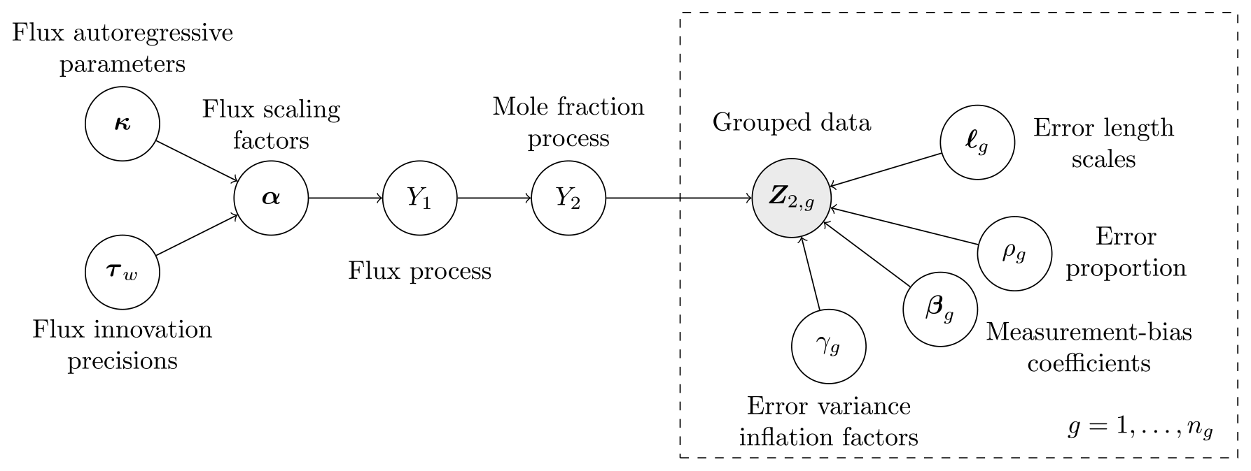
Figure 1Graphical model summarising the relationship between the variables, processes, parameters to be inferred, and the grouped data .
The joint posterior distribution over all quantities can be estimated using a Gibbs sampler, which successively “updates” parameters using their full conditional distributions. When the conditional distributions cannot be sampled from directly (in particular, for the parameters κ, ℓg, and ρg, for ), we employ a slice sampler (Neal, 2003) to obtain samples. Details are given in Appendix A.
The posterior distribution over all the unknown parameters in our model is given by
The log of the first two terms on the right-hand side of Eq. (10) are expressions that are commonly seen in optimisation-based flux-inversion frameworks. In particular, we have
where ; in our case we set αp=0, and “const.” denotes a constant. The primary differences between our framework and the usual optimisation-based flux-inversion frameworks are the presence of the log determinants, which penalise covariance matrices that have large determinants (large correlations and/or large variances), and the presence of off-diagonal elements in the matrix Σξ+Σϵ. Note that the log determinants can only be omitted when all covariance matrices are considered known a priori.
The computational complexity of the Gibbs sampler is dominated by that of the log-likelihood function, which is the sum of the group-wise log-likelihood functions, , for . For computationally efficient inference, we must ensure that each group-wise log-likelihood function is simple to evaluate. From Eq. (9), the group-wise log-likelihood is given by
for , where and mg is the number of observations and/or retrievals in group g. From a computational perspective there are two components in Eq. (11) that can present difficulties. The first component is the matrix ; this matrix is dense, and its number of elements scales linearly with both the number of data points and the number of basis functions, r. Fortunately, this matrix only needs to be evaluated once using the CTM, and it can typically be generated efficiently on a large parallel computing infrastructure. The second component is the matrix Σg, which is of size mg×mg and generally dense. Recall from Sect. 2.4 that this covariance matrix is constructed from and ρg, which are sampled within the Gibbs sampler. Therefore, this covariance matrix needs to be re-constructed at each sampler iteration. This is infeasible for the mg≈100 000 retrievals used in this study.
We deal with the denseness of Σg by using an approximation first proposed by Vecchia (1988). Here, one first orders the elements of ξg. Following this, one approximates the joint distribution of ξg as,
where 𝒩g,i is the “past” neighbour set of the ith datum in group g, which contains a (very small) subset of the integers between, and including, 1 and (i−1). It can be shown that this formulation leads to a valid distribution for ξg that approximates the true joint distribution. The approximate distribution is Gaussian with mean 0 and a sparse precision matrix, , with the degree of sparsity closely connected to the sizes of the sets .
In the version of WOMBAT presented here, we consider a special case of Eq. (12), where the observations are ordered in time and where the correlation function is simply an exponential function of temporal separation. In this case, one only needs to consider one (temporal) length-scale parameter per group, for . The motivations for this simplification are twofold. First, the remote sensing instrument we consider in Sect. 5 flies on a satellite that is in a sun-synchronous orbit, and thus correlation in time is a proxy for along-track correlations. This model for characterising correlation in the errors was suggested and used by Chevallier (2007). Second, the use of an exponential correlation function allows the approximation in Eq. (12) to become an equality, where . This is a manifestation of the so-called “screening effect”, where the exponential correlation function induces a first-order conditional-independence structure. Now, and , where is very sparse and is diagonal. Efficient computations of Eq. (11) therefore follow by expressing and in terms of these sparse matrices. Specifically, and are evaluated through the use of the Sherman–Morrison–Woodbury matrix identity and a matrix-determinant lemma (e.g. Henderson and Searle, 1981, and Appendix A).
This section gives the setup needed for Sect. 5, where we compare the inversions from WOMBAT v1.0 to those from the OCO-2 MIP (Crowell et al., 2019). In the MIP, inversions followed a predefined protocol; we therefore configured WOMBAT to follow the same protocol. The MIP prescribed the data to be used, including both preprocessed point-referenced data and remotely sensed data from OCO-2 between 6 September 2014 and 1 April 2017. Participants were tasked to provide flux estimates for the years 2015 and 2016. The protocol also specified a fossil-fuel flux field that had to be assumed fixed and known, in order to facilitate the interpretation of the differences in flux estimates obtained by the different participants. All other modelling choices (e.g. transport model, prior fluxes) were left to individual participants.
4.1 Prior expected flux
Our prior expectation of the spatio-temporal flux process, , is constructed from inventories of different types of fluxes through the following decomposition:
where corresponds to fossil-fuel emissions, to terrestrial biospheric fluxes, to biofuel emissions, to fire emissions, and to ocean–air exchange fluxes. We now describe these components in more detail.
-
Fossil-fuel emissions. For we use the Open-source Data Inventory for Anthropogenic CO2 monthly fossil-fuel emissions (ODIAC2016; Oda and Maksyutov, 2011; Oda et al., 2018) with Temporal Improvements for Modeling Emissions by Scaling (TIMES) weekly scaling factors (Nassar et al., 2013). This term also includes emissions from international aviation and shipping. The fossil-fuel fluxes are prescribed by the MIP protocol.
-
Biospheric flux. This flux is a result of the interaction between the atmosphere and trees, shrubs, grasses, soils, dead wood, leaf litter, and other biota. It is defined by the quantity , where GPP stands for gross primary production (the uptake of carbon by plants due to photosynthesis), RA is autotrophic respiration (the release of carbon through respiration by plants), and RH is heterotrophic respiration (the release of carbon through the metabolic action of bacteria, fungi, and animals). For we use one of the two priors used in CarbonTracker 2019 (Jacobson et al., 2020), specifically that based on the Carnegie–Ames–Stanford Approach (CASA) biogeochemical model (Potter et al., 1993; Giglio et al., 2013).
-
Biofuel emissions. These emissions result from the burning of wood, charcoal, and agricultural waste for energy, as well as the burning of agricultural fields. For we use the estimates of Yevich and Logan (2003) that in turn were based on data from 1985.
-
Fire emissions. These emissions correspond to those from vegetative fires (wildfires), which may either start naturally or be started by humans. For we use the Quick Fire Emissions Dataset, version 2 (QFED2; Darmenov and da Silva, 2015).
-
Ocean–air exchange. These fluxes are a result of ocean–air differences in partial pressure of CO2. For we use the estimates of Takahashi et al. (2002), with annual scalings reflecting increasing uptake of CO2 as described by Takahashi et al. (2009).
A summary of these components is provided in Table 1.
Oda and Maksyutov (2011)Nassar et al. (2013)Oda et al. (2018)Potter et al. (1993)Giglio et al. (2013)Jacobson et al. (2020)Yevich and Logan (2003)Darmenov and da Silva (2015)Takahashi et al. (2002, 2009)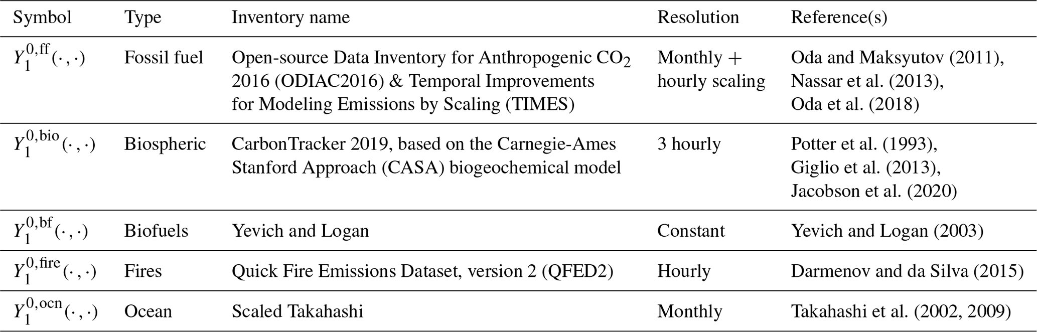
4.2 Basis functions
We divided the globe into the rs=22 disjoint TransCom3 regions (Gurney et al., 2002) and time into the rt=31 months between (and including) September 2014 and March 2017, and then we constructed one flux basis function for each region–month pair. This yielded basis functions, each with non-zero support in a space–time volume spanning 1 month in time, and one TransCom3 region in space. Half of the TransCom3 regions are land regions and half are ocean regions, and thus half of our basis functions correspond to land areas and half to ocean areas. We show the TransCom3 regions in Fig. S1 and their codes and labels in Table S1, both of which can be found in the Supplement. Some areas of the globe, depicted in white in Fig. S1, are assumed to have zero flux; all of our basis functions are zero in these regions.
For , a basis function corresponding to a land area, we have
where is the space-time volume over which the jth basis function is defined to be non-zero. For a basis function corresponding to an ocean area, we have
Both Eqs. (14) and (15) exclude . This is done to meet the MIP requirement that fossil-fuel fluxes are treated as fixed and known (which is common practice in flux inversion; see, e.g. Basu et al., 2013). The influence of fossil fuels on the mole-fraction field is therefore present only as an invariant component of the prior expectation of the mole-fraction field. Note that we have used the same inventories to construct and the basis functions ; this was done for convenience, and different inventories could be used if needed.
Since the spatio-temporal patterns of the fluxes within a region–month space–time volume are fixed, our construction is quite restrictive. However, the space–time patterns are dictated by those in the inventories used to construct the basis functions. Although there is a general lack of agreement between inventories targeting the same processes (e.g. Huntzinger et al., 2017), these spatio-temporal patterns would not be unreasonable and certainly more reasonable than those from generic basis functions commonly used in spatial statistics (e.g. Wikle et al., 2019, chap. 4). This underlying assumption is often made in flux-inversion systems; for example, Jacobson et al. (2020) scale 3-hourly fluxes using weekly scale factors over 156 regions, while Basu et al. (2013) use monthly scale factors for 3-hourly fluxes over grid cells. Constraining the spatio-temporal pattern is inferentially advantageous because it helps address the ill-posed nature of flux inversion. It is also computationally advantageous because it reduces the number of unknowns for which inference is needed. The disadvantage is that the reliance on a priori structures increases the risk of dimension reduction error because, while our basis functions allow the posterior fluxes to vary at sub-TransCom3-region scales, variations that do not follow the prescribed pattern are necessarily ignored. Therefore, if one wishes to make inference at scales that are finer than those resolved by the scaling factors, one should introduce additional basis functions for those regions and time spans. Moreover, for processes where there is disagreement (such as biogeochemical processes), one may consider running separate inversions with basis functions constructed from different inventories and carry out a sensitivity analysis. We note that there is a considerable body of work tackling basis-function choice in the context of inversion; see, for example, Turner and Jacob (2015).
As described in Sect. 2.2, for , each flux basis function has a corresponding mole-fraction basis function , which may be constructed by running the transport model, , under the flux . Then the mole-fraction basis function is recovered through linearity by simply subtracting from the output mole-fraction field. For illustration, Fig. 2 shows examples of the flux basis functions (monthly averaged) for January 2016 and the regions TransCom3 02 and TransCom3 06, and it also shows snapshots of the corresponding mole-fraction basis functions (daily and atmospheric-column averaged) obtained using the transport model described next in Sect. 4.3.
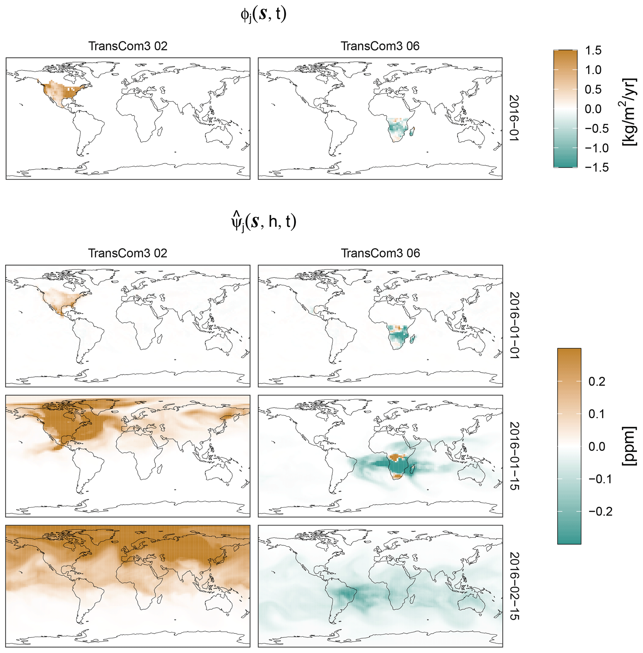
Figure 2Examples of flux basis functions that have support in the month of January 2016 in the regions TransCom3 02 and TransCom3 06 and the corresponding mole-fraction basis functions. The first row shows the values of the flux basis functions, , averaged over the whole month (these basis functions are zero outside January 2016). The next three rows show daily averages of the column-averaged CO2 for the corresponding mole-fraction basis functions on 3 different days: the start of the month-long period where the flux is non-zero, 1 January 2016; the middle of the period, 15 January 2016; and 15 d after the end of the period, 15 February 2016.
4.3 Transport model and initial condition
For our approximate transport model, , we used the GEOS-Chem global 3-D chemical transport model, version 12.3.2 (Bey et al., 2001; Yantosca, 2019), driven by the GEOS-FP meteorological fields from NASA's Goddard Earth Observing System (Rienecker et al., 2008). We use the offline GEOS-Chem CO2 simulation (Nassar et al., 2010), with the native horizontal resolution of and 72 vertical levels aggregated to and 47 vertical levels for computational efficiency. We use a transport time step of 10 min and a flux time step of 20 min. All fluxes described in Sects. 4.1 and 4.2 were implemented in GEOS-Chem using the HEMCO emissions component (Keller et al., 2014). GEOS-Chem can be configured to allow for a 3-D chemical source of CO2 due to oxidation of other trace gases, but this was disabled for compatibility with the OCO-2 MIP.
The approximate initial condition, , specifies the mole-fraction field at the beginning of the study period on 1 September 2014. For our initial mole-fraction field, we used a modified version of that generated by Bukosa et al. (2019). This mole-fraction field was constructed using a spin-up period, starting on 1 January 2005 and ending on 1 September 2014, with transport driven by inventory fluxes and meteorology (that in some cases differ from those we use here; see Bukosa et al., 2019, for details). At the end of the spin-up period, the whole mole-fraction field on 1 September 2014 was scaled such that the value in the surface grid cell containing the South Pole was equal to the monthly averaged mole-fraction measurement from surface flask measurements at the South Pole (Thoning et al., 2020) in September 2014. The South Pole was chosen as our calibration point due its physical isolation from strong sources and sinks.
4.4 Data
This study uses a subset of the data sources in the MIP (Crowell et al., 2019). These include retrievals of column-averaged CO2 by NASA's OCO-2 satellite (Eldering et al., 2017) and retrievals of column-averaged CO2 from TCCON (Wunch et al., 2011a). As in the MIP, we use OCO-2 data to estimate CO2 fluxes and TCCON data to validate the estimates.
4.4.1 OCO-2
The OCO-2 satellite was launched in 2014 with the goal of retrieving atmospheric CO2 mole fractions. The on-board instrument measures radiances in three near-infrared spectral bands, which in turn are used to retrieve the CO2 mole fraction on 20 vertical levels via a retrieval algorithm based on Bayesian optimal estimation (Rodgers, 2000; O'Dell et al., 2012). The retrieved levels are column-averaged and then bias-corrected through comparison with TCCON retrievals (Wunch et al., 2011a). The OCO-2 team releases regular revisions of the retrieval dataset.
OCO-2 radiance measurements are taken in three distinct pointing modes: nadir mode, where the satellite aims at the point directly beneath it; glint mode, where the satellite points at the reflection of the sun on the surface; and target mode, where the satellite aims at a specific target, typically a ground station that also measures CO2 mole fractions. Target observations are generally excluded from flux inversions and used only for instrument calibration. Over the ocean, nadir measurements have insufficient signal-to-noise ratio to provide useful retrievals, while over land both nadir and glint retrievals are made. There are therefore three retrieval modes to consider, land glint (LG), land nadir (LN), and ocean glint (OG). The error properties of retrievals over land differ significantly from those over ocean; in particular, the OG retrievals in the V7r dataset (the dataset used in the MIP) are not considered reliable and were therefore excluded from the MIP (Crowell et al., 2019). We follow this protocol and only do inversions using LG and LN data.
The MIP protocol dictated the use of a post-processed version of the V7r retrievals; this post-processing was done as follows. First, an additional bias-correction term related to high-albedo measurements was applied to the XCO2 retrievals. The bias-corrected retrievals were then grouped and averaged into 1 s bins, and following this they were further grouped and averaged into 10 s bins. The 10 s spans correspond to ground swathes of approximately 67 km in length. The standard deviation for each 10 s retrieval was computed as a function of the individual retrieval standard deviations, with an additional model–data mismatch term added to account for the expected differences arising from transport model errors. For the MIP, the 10 s averages were assumed to be independent but, following Sect. 2.4, we treat them as dependent. For more details on how the 10 s averages were computed, including how the standard errors were derived, see Crowell et al. (2019).
The OCO-2 retrieval algorithm produces estimates of XCO2. In Eq. (7), we encapsulate the retrieval algorithm in the observation operator, . Appendix B gives more details on this observation operator in the case of OCO-2 retrievals.
4.4.2 TCCON
TCCON is a network of ground-based sites measuring solar radiances in the near-infrared spectral band (Wunch et al., 2011a). Similar to the way OCO-2 retrievals are obtained, these measurements are converted to retrievals of column-averaged CO2 (and other gases) using a retrieval algorithm. TCCON retrievals have been adjusted to agree with World Meteorological Organization (WMO) trace-gas measurement scales, and validated using aircraft data (Wunch et al., 2010). As both TCCON and remote sensing instruments retrieve column-averaged mole fractions, the TCCON data are an important validation resource (Wunch et al., 2011b). The MIP used TCCON column-averaged CO2 retrievals from the GGG2014 release as validation data, including all retrievals available as of 6 July 2017. In the MIP, outliers and retrievals corresponding to retrievals with high solar zenith angle were removed. The remaining TCCON retrievals were then averaged over 30 min intervals; further details are given by Crowell et al. (2019). We note that the filtering procedure used in the MIP occasionally led to long periods of time for which data were considered missing. For consistency with the MIP, in this study we used the same retrievals and postprocessing methods; the stations used are listed in Table 2.
Feist et al. (2014)Deutscher et al. (2015)Notholt et al. (2014)Wennberg et al. (2015)Griffith et al. (2014a)Iraci et al. (2016)Strong et al. (2016)Blumenstock et al. (2014)Hase et al. (2015)Wennberg et al. (2016)Sherlock et al. (2014)Dubey et al. (2014)Warneke et al. (2014)Wennberg et al. (2014)De Mazière et al. (2014)Kawakami et al. (2014)Kivi et al. (2014)Morino et al. (2016)Griffith et al. (2014b)
Like OCO-2, TCCON retrievals also have an associated observation operator . This has a similar form to the operator for OCO-2, which is described in Appendix B. A detailed description of the TCCON observation operator is given by Wunch et al. (2011b).
4.5 Prior distributions over the parameters
The prior distributions for the parameters governing the scaling factors, α, are specified separately for the land and ocean TransCom3 regions. The land regions, which are observed directly by OCO-2 when in LG or LN mode, are assigned a non-informative prior, while the indirectly observed ocean regions (which also have relatively small fluxes over a given area) are assigned a relatively informative prior. Informative priors for ocean fluxes were deemed necessary following OSSEs performed by us that revealed that it is often not possible to reliably constrain ocean fluxes from OCO-2 land data.
Specifically, for j corresponding to a land region, we assigned a prior to κj by letting (resulting in a uniform prior over [0,1]), and for τw,j we let and . This prior on τw,j implies that , the marginal variance of the elements of the scalings in α that correspond to land regions, has 5 % and 95 % percentiles of 0.01 and 10, respectively, which is reasonably uninformative. For j corresponding to an ocean region, we apply an independent and identically distributed Gaussian prior with mean zero and standard deviation of 0.5 to αj. This is achieved by fixing κj=0 and .
As described in Sect. 4.4.1, the OCO-2 MIP 10 s averages come with prescribed uncertainties that include both measurement error and transport model error. In our framework, the parameters governing these error processes are γg, ρg, and ℓg,1. For the prior distribution of γg, we let and , which lead to 5 % and 95 % prior percentiles of 0.5 and 10, respectively, while we used a uniform prior distribution on [0,1] for ρg. For ℓg,1, we let and . When doing bias correction online, we used the prior on β described in Sect. 2.4.
4.6 Computation
Computations were performed in two stages. In the first stage, the 682 mole-fraction basis functions were precomputed in the manner described in Sect. 4.2. This is the most computationally demanding step, as each basis function requires the CTM to be run for several days of clock time, on average. Fortunately, since every basis function can be computed independently from all others, computing them is an embarrassingly parallel problem. Furthermore, since the basis functions are shared between the different inversions in this section, they only need to be computed once. Computation of the basis functions took 7 d in total using the Gadi supercomputer at the Australian National Computational Infrastructure.
The inversions were performed in the second stage. As mentioned in Sect. 2.5, the posterior distribution for each inversion was estimated using an MCMC sampling scheme, with details given in Appendix A. The sampling schemes in all cases were run for 11 000 iterations, and the first 1000 iterations were discarded as burn-in. Convergence of the MCMC chain was confirmed by inspection of all the trace plots. In our studies, we found that the vast majority of posterior distributions were different from the prior distributions, and this is not surprising. Although complex, the model used in WOMBAT is low-dimensional, and in this setup the total number of unknowns is 732 (r=682 of which are flux scaling factors), which is orders of magnitude less than the number of LG and LN data available for the inversion (114 808 and 129 203, respectively). Specifically, these data prove to be highly informative of the unknown parameters in our model. Generally, one need not be overly concerned if a parameter is poorly constrained by the data. In such cases, a Bayesian framework such as WOMBAT returns a posterior distribution over the poorly constrained parameter that tends toward the prior distribution, which in turn encapsulates the a priori belief on the plausible range of values the parameter can take.
The MCMC scheme was implemented in the R programming language (R Core Team, 2020), with intensive linear algebraic computations offloaded for performance to a graphics processing unit (GPU) using Tensorflow (Abadi et al., 2016). The total running time of the sampler depended on which model assumptions were used; specifically, whether uncorrelated (15 min) or correlated errors (2 h) were modelled. The bottleneck leading to a drastic increase in computing time when modelling correlated errors is due to the term in Eq. (A7), which needs to be re-evaluated at each MCMC iteration. This operation scales as O(r3+nr2); on hardware current to the year 2021, r needs to be less than 10 000 for computations to remain tractable. On the other hand, when the errors are assumed to be uncorrelated or the length-scale parameters are assumed known, many matrix computations can be done only once (and not at each MCMC iteration); in this case the bottleneck becomes memory, and on current state-of-the-art servers one may accommodate an order of magnitude more basis functions. All inversions were performed on a machine with an eight-core Intel i9-9900K CPU running at 3.60 GHz and an NVIDIA RTX 2080 GPU.
In this section we evaluate WOMBAT, first in an OSSE, where the true fluxes are assumed known and data are simulated from these true fluxes, and then on actual satellite data via the MIP protocol of Crowell et al. (2019). Using an OSSE, described in Sect. 5.1, serves two purposes: first, to show that WOMBAT can indeed recover the true fluxes in a controlled environment where the “working model” is the “true model”, and second to illustrate the importance of modelling measurement error biases and correlated errors when these are present in the true model from which the data are simulated. Following this, in Sect. 5.2 we show that WOMBAT gives similar flux estimates to those obtained by different MIP participants and that it performs well relative to the MIP participants in reproducing out-of-sample TCCON validation data. In Sect. 5.3 we show that WOMBAT is able to estimate bias coefficients online, if needed.
5.1 Observing system simulation experiment (OSSE)
In this section we illustrate the use of WOMBAT in an OSSE, where we randomly draw flux scaling factors αs from a Gaussian distribution with mean 0 and covariance matrix 0.09I, and assume that these are the true flux scaling factors. The (simulated) true flux is given by
where is the jth element of αs. The (simulated) true mole-fraction field, , is then given by
Finally, we simulate measurements from the mole-fraction data model in Eq. (9) at the same times and locations as the OCO-2 10 s average retrievals for the LN and LG modes by passing through the corresponding OCO-2 observation operators (see Sect. 4.4.1).
When simulating data via Eq. (9), we assume that both bg and ξg are present. For the bias term bg, we assume that the OCO-2 retrieval biases are a linear combination of covariates that are associated with bias in the retrieval process:
-
“dp” is the prior–retrieval surface pressure differential;
-
“logDWS” is the logarithm of the total retrieved optical depth associated with the aerosol types dust, water cloud, and sea salt;
-
“co2_grad_del” is the difference between the retrieved CO2 mole fractions at the surface and retrieval vertical level 13 (corresponding to the height with air pressure equal to 63.2 % of the surface pressure, which is around 520 to 650 hPa for most retrievals).
The “official” V7r bias-correction parameters (regression coefficients) for the original Level 2 (L2) data release were obtained through offline comparison of the raw L2 product with TCCON retrievals, and they are the same for both LG and LN observations. They are equal to 0.3, 0.028, and 0.6 for the three variables, respectively. We construct our (simulated) true biases based on these coefficients.
As discussed in Sect. 2.4, we assume that the prescribed variance of each retrieval needs to be inflated, and the inflated variance is the sum of the variance from both the correlated (ξg) and uncorrelated (ϵg) error components. In our OSSE, we assume that the inflation factor of the prescribed variances, , is γg=1.25, and that the proportion of this variance allocated to the correlated error process is ρg=0.8. We induce the correlations using the exponential covariance function described in Sect. 3 with the single length scale of the correlated component set to min for all . We specify this correlation structure to be the same for both LG and LN data.
We ran five different setups in WOMBAT. In four of these setups, bias is assumed or not assumed to be present, errors are assumed or not assumed to be correlated, and all model hyperparameters are estimated. The fifth setup attempts to mimic a conventional flux inversion system based on scaling factors; here data is assumed to be unbiased, the errors uncorrelated, and the hyperparameters fixed to their true values. The known true flux, generated as described above, is the same between the cases, and we evaluate the ability of WOMBAT to recover the truth under each of the setups. Table 3 gives the root-mean-squared error (RMSE) and continuous ranked probability score (CRPS, Gneiting and Raftery, 2007) when estimating monthly and regionally aggregated fluxes using these five setups. The regions on which these evaluations are based are the same TransCom3 regions that were used to construct the flux basis functions (see Sect. 4.2), and the quantities in the table are averages across all combinations of the 31 months and 22 regions. The true data-generating process involves both bias and correlated error. Therefore, as one would expect, Table 3 shows that the WOMBAT setup that takes into account both of these features performs the best in terms of both RMSE and CRPS, while the setups that assume that neither feature is present perform the worst. For the two partially misspecified setups, the bias-corrected and uncorrelated setup outperforms the not-bias-corrected and correlated setup for LG data, while the opposite is true for LN data. Notably, despite the presence of systematic biases in the simulated data, the WOMBAT setup that assumes no bias, but which takes into account correlated errors, performs overwhelmingly better than the fully misspecified model that assumes no bias and uncorrelated errors, where the hyperparameters are assumed to be unknown. The performance of the setup with hyperparameters fixed to their true values is between those of the fully and the partially misspecified setups, illustrating the importance of modelling and estimating biases and correlations when these are indeed present.
Table 3Root-mean-squared error (RMSE) and continuous ranked probability score (CRPS) when estimating monthly regional fluxes using LG and LN data in the OSSE of Sect. 5.1. The lower the error or the score, the better the performance. Five setups in WOMBAT are evaluated, and the regions and time periods over which these summaries (averages) are obtained are the same as those used for constructing flux basis functions (see Sect. 4.2).

Figure 3 shows the (simulated) true (black), prior mean (blue), and posterior distributions (red, purple, orange, light green, and dark green) for the total flux in the tropics (latitude 23.5∘ S to 23.5∘ N) in 2015 and 2016 from both LN and LG and split by the southern and the northern components (latitudes 23.5∘ S to 0∘ and 0 to 23.5∘ N, respectively). The five posterior distributions depicted in each panel correspond to the five different WOMBAT setups. The interior of the ellipses represent the 95 % credible regions. The dotted grey lines along the diagonal correspond to combinations of the southern and northern fluxes that yield the true total flux in the tropics; if the dotted line is not within the ellipse for an inversion, the total flux is mis-estimated. All fluxes shown in Fig. 3 are exclusive of fossil fuels which, recall, are held fixed in the inversions. Figure S2 shows the results on a global scale (land vs. ocean), while Fig. S3 shows the results on a regional scale: TransCom3 region 04 (South American Temperate) vs. TransCom3 region 06 (Southern Africa) .
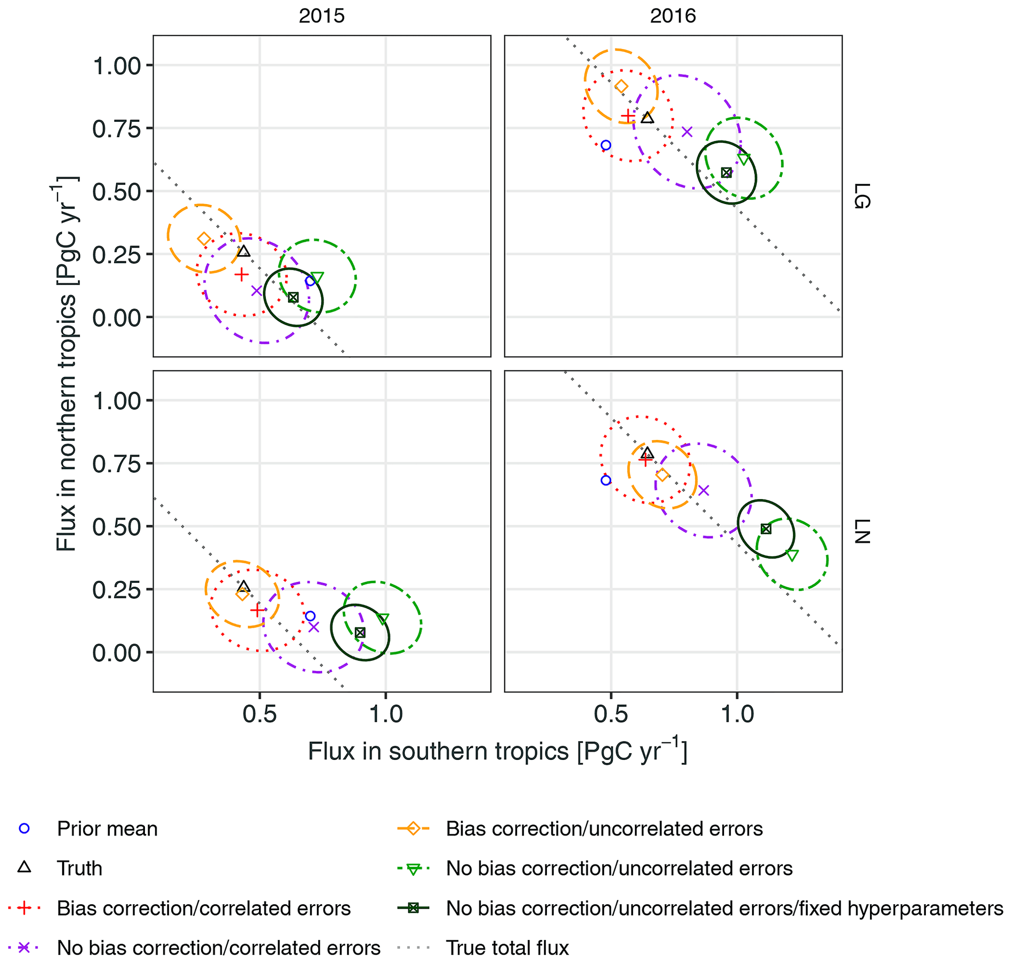
Figure 3True, prior, and posterior estimates of total flux in the northern tropics (0 to 23.5∘ N) vs. the total flux in the southern tropics (23.5∘ S to 0∘) for the OSSE in Sect. 5.1. The columns correspond to the years 2015 and 2016, while the rows show which observation groups were used, either OCO-2 land glint (LG) or land nadir (LN), noting that the prior and true flux are the same across rows. Points show the posterior mean fluxes for each model configuration, as well as the prior mean in blue and the truth in black. The ellipses contain 95 % of the posterior probability for the true tropical fluxes in the Southern Hemisphere and the Northern Hemisphere. The dotted grey lines along the diagonal correspond to combinations of southern and northern tropical fluxes that yield the true total flux in the tropics. All fluxes are exclusive of fossil fuels, which are held fixed in the inversion.
Collectively, the performances of the different models, as shown in Figs. 3, S2, and S3, align with the conclusions based on the RMSE and CRPS statistics. In all the cases shown, the 95 % credible regions for the WOMBAT configuration with both bias correction and correlated error (red) contain the true value, while those for the configuration with neither feature (light green and dark green) do so rarely. The orange credible regions for the bias-corrected and uncorrelated variant are always smaller than the red credible regions, indicating that the bias-corrected and uncorrelated variant is overconfident. In contrast, the purple credible regions for the not-bias-corrected and correlated variant are always larger, which may suggest that the correlated errors are partially compensating for the lack of bias correction in this variant.
In summary, this OSSE shows that WOMBAT can recover the true flux when the assumed model is the true model, but more importantly the OSSE also demonstrates the importance of modelling both bias and correlated errors in these flux inversions. If the bias parameters are omitted, fluxes can be estimated incorrectly, although this may be partially mitigated by modelling correlated errors. If uncorrelated errors are assumed, estimation performance suffers, and flux estimates will likely be reported with too small an uncertainty, even if the prescribed variances are allowed to be inflated when making inference. In a real-data setting, any factors thought to introduce systematic biases should be taken into account, but this OSSE also suggests that the use of correlated errors may provide some insurance against any remaining unmitigated spatio-temporal biases.
5.2 OCO-2 satellite data
In this section we present results from WOMBAT applied to OCO-2 satellite data under the MIP protocol (Crowell et al., 2019). The protocol mandates the use of OCO-2 retrievals with the TCCON-based offline bias correction. While WOMBAT is capable of online bias correction (see Sect. 5.3), in this section we follow the MIP protocol and set the bias parameters in WOMBAT equal to zero.
5.2.1 Flux comparison on a region–time basis with the MIP
In the OCO-2 MIP, nine participants submitted fluxes based on inversions satisfying the MIP protocol. Each participant reported to the MIP four sets of fluxes: their prior mean fluxes and their fluxes from three inversions based on point referenced data, OCO-2 LG data, and OCO-2 LN data, respectively. Crowell et al. (2019) considered the different participants' fluxes as an ensemble, reporting the ensemble mean, median, and standard deviation across a variety of temporal and spatial scales. Under the same protocol and using OCO-2 LG and OCO-2 LN data, we compare WOMBAT's posterior distribution over the fluxes to the corresponding results from the MIP ensemble.
Through its MCMC Bayesian computations, WOMBAT's inversions generate samples from the posterior distribution of all unknown quantities in the model, including the parameters discussed in Sect. 2.4. Section 5.2.3 discusses the inferred parameters in detail for inversions corresponding to different satellite modes. Of note are the posterior distributions of the parameters {ρg}, which are centred on values around 0.84. This is a strong indication that the majority of the process that combines model–data discrepancy and measurement error should indeed be attributed to the correlated component, ξg, given in Eq. (9). Samples from the MCMC scheme enable estimation of functionals of the posterior distribution, including posterior means and quantiles, of the flux process . While some individual MIP participants are able to produce probabilistic uncertainty estimates for fluxes, these were not reported as part of the MIP; instead, the empirical distribution from the ensemble of fluxes was used by the MIP for uncertainty quantification. Since it is difficult to make a quantitative comparison between WOMBAT's posterior-based uncertainties and the ensemble uncertainties in the MIP, we opt here for a visual comparison of the posterior means and standard deviations over the fluxes compared to the ensemble minimum, mean, and maximum. This comparison is done at both annual and monthly temporal scales, and across spatial scales encompassing the whole globe, global land, global ocean, and zonal bands.
Global totals. Figure 4 presents annual and monthly non-fossil-fuel fluxes for the globe, land regions, and ocean regions for inversions using the LG retrievals. Fluxes are shown for the MIP, split into prior and LG inversions, and for WOMBAT they are split into prior and posterior using LG data. Thick lines show the ensemble means for the MIP, and the (prior or posterior) means for WOMBAT. Shaded areas and thin lines for the MIP denote the values between the ensemble minimum and maximum, while for WOMBAT they denote values in the 95 % fully Bayesian credible intervals. The corresponding figure for LN inversions is given in Fig. S4.
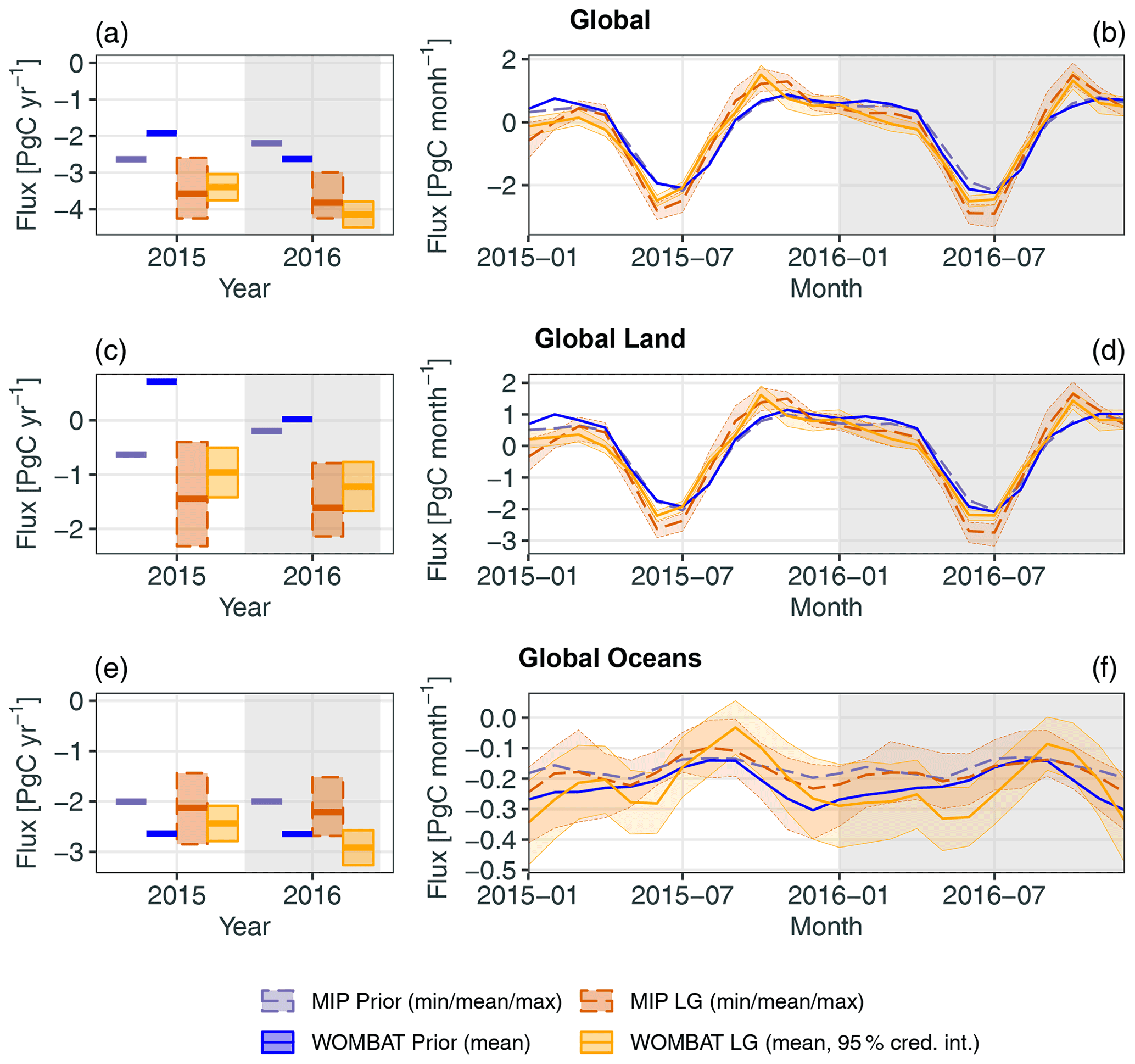
Figure 4Annual (a, c, e) and monthly (b, d, f) fluxes for the globe (a, b), land (c, d), and ocean (e, f). Summaries of flux estimates from the MIP and the flux estimate from WOMBAT are shown, split into the prior and LG inversions. Thick lines represent the ensemble means for the MIP and the (prior or posterior) means for WOMBAT. Shaded areas and thin lines for the MIP represent values between the ensemble minimum and maximum, while for WOMBAT they represent values in the 95 % credible intervals (cred. int.). Fossil-fuel fluxes are excluded from all figures. Note that each row of plots has a different vertical scale.
The global annual non-fossil-fuel fluxes estimated by posterior means from WOMBAT are very similar for both LG and LN modes, with an overall posterior mean net sink in 2015 of 3.40 and 3.14 PgC yr−1 for LG and LN, respectively, and in 2016 of 4.14 and 4.27 PgC yr−1 for LG and LN, respectively. For 2015, these sinks are very similar to the MIP ensemble means (3.57 and 3.21 PgC yr−1 for LG and LN, respectively). However, for 2016, WOMBAT returns a larger posterior-mean sink than the MIP ensemble means (3.82 and 3.78 PgC yr−1 for LG and LN, respectively), and its 95 % credible intervals do not contain the ensemble means within them. At a monthly scale, WOMBAT reproduces a key feature of the MIP fluxes, wherein the seasonal cycle in the fluxes, driven by the Northern Hemisphere growing season, begins and ends earlier than it does in the prior for both 2015 and 2016. In agreement with the MIP, WOMBAT results indicate that the largest sink in the cycle is larger than that in the prior. However, the sink estimated by WOMBAT is around 0.4 PgC per month smaller than the MIP ensemble mean for both LG and LN and for both 2015 and 2016.
Global land and ocean. For global land fluxes, shown in the second row of Figs. 4 and S4, WOMBAT's results agree with those from the MIP for both LG and LN in that a source larger than that in the prior flux is estimated for October 2015. However, while the source persists into November in the MIP ensemble mean, the WOMBAT posterior mean does not have the same persistence. For global ocean fluxes, shown in the third row of Figs. 4 and S4, the MIP LG-estimated and LN-estimated fluxes differ little from the prior fluxes, and we observe the same for global oceans in the WOMBAT estimates for both LG and LN modes and in most months. The exceptions are September and October in both years, where WOMBAT estimates a shallower sink, and even zero flux with the LN data. These features are not obvious in the MIP ensemble means, but they do appear reasonable within the MIP ensemble spread.
Zonal bands. Figures S5 and S6 show for LG and LN inversions, respectively, fluxes for zonal bands covering the northern extratropics (23.5 to 90∘ N), northern tropics (0 to 23.5∘ N), southern tropics (23.5∘ S to 0∘), and southern extratropics (90 to 23.5∘ S). For the MIP ensemble, Crowell et al. (2019) noted that inversions using LG data led to a smaller net annual sink (averaged between 2015 and 2016) in the northern extratropics than those using LN data. WOMBAT also finds this feature, with a 95 % credible interval of the LG-minus-LN difference spanning 0.14–0.6 PgC yr−1. This is substantially smaller than the difference between the MIP ensemble means for these modes, which is 0.7 PgC yr−1. Fluxes in the southern extratropics, shown in the fourth row of Figs. S5 and S6, are dominated by ocean fluxes for which, as noted above, LG and LN data provide little information.
One of the most prominent features in the MIP inversion results is a seasonal cycle in the tropics that is larger than that in both the prior mean and the in situ inversions (Crowell et al., 2019). From the second and third rows of Figs. S5 and S6, which depict inferred tropical-zone fluxes, it can be seen that WOMBAT does not reproduce this feature for both LG and LN inversions. In the northern tropics, the WOMBAT posterior means are similar to the prior means, and the credible intervals in the annual fluxes reflect high confidence. However, results from WOMBAT do corroborate those of the MIP ensemble, in that non-fossil-fuel fluxes in the northern tropics were a net source of CO2 in 2016.
5.2.2 TCCON comparison
To evaluate the estimated fluxes in the OCO-2 MIP, each participant was asked to use the 30 min average TCCON retrievals of column-averaged CO2 (see Sect. 4.4.2) as validation data, and compare them to the column-averaged CO2 predicted values obtained by applying the process model to the estimated fluxes with the same CTM used for the inversion. Recall that when performing the inversions only OCO-2 data were used and that the TCCON data were treated as unobserved and set aside for validation. For WOMBAT, we repeated this validation exercise by examining the prior and posterior distributions of Z2,g, where each g corresponds to a different TCCON site. For each group g, we set bg=0, since we assume that the TCCON retrievals provided are free of bias. On the other hand, we assumed that ξg+ϵg has variance that is group specific and that these errors are fully correlated. While this assumption is conservative, it is also reasonable, since the CTM does induce errors that are highly correlated in time at a common spatial location, as it averages all variables on a rather coarse grid when simulating atmospheric transport. We estimate the variance of these correlated errors in a group g as the average of the reported variances of each TCCON retrieval within the gth group.
In Fig. S7, we compare the time series of the TCCON retrievals with the predictions from WOMBAT under the prior-mean flux, the posterior distribution of flux from LG data, and the posterior distribution of flux from LN data. Several things are of note from this figure: first, the posterior-mean estimates are a better match to the TCCON retrievals than the prior-mean estimates, which is evidence that OCO-2 data do allow for improved flux estimates to be obtained. Second, discrepancies between TCCON and predicted retrievals persist for a long time, lending credence to our assumption that errors are highly temporally correlated. Third, the 95 % prediction intervals are appropriate, and largely contain the TCCON retrievals.
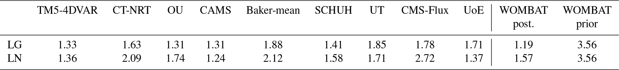
In Fig. 5, we reproduce an augmented version of Fig. 8 of Crowell et al. (2019), which depicts the mean and standard deviation of the differences between the TCCON retrievals and the predicted retrieval by TCCON site, MIP participant, and observation mode (LG and LN) alongside the results from WOMBAT. The improvement of the WOMBAT posterior prediction over the prior prediction is evident in the mean of the differences, and the posterior error means and standard deviations of WOMBAT are in line with those of the MIP participants. WOMBAT's predictive distributions from LG-inferred fluxes can be seen to be better than those of the MIP participants, even by straightforward visual inspection. In Table 4 we compute mean-squared error, by participant and observation mode, averaged over the 19 TCCON stations used in the MIP. WOMBAT outperforms all other participants when using this metric with LG data, and it is the fourth best when using this metric with LN data. While these results are not conclusive on the validity of the WOMBAT fluxes globally, they are encouraging, especially in light of the fact that our flux process has a relatively low-dimensional representation.
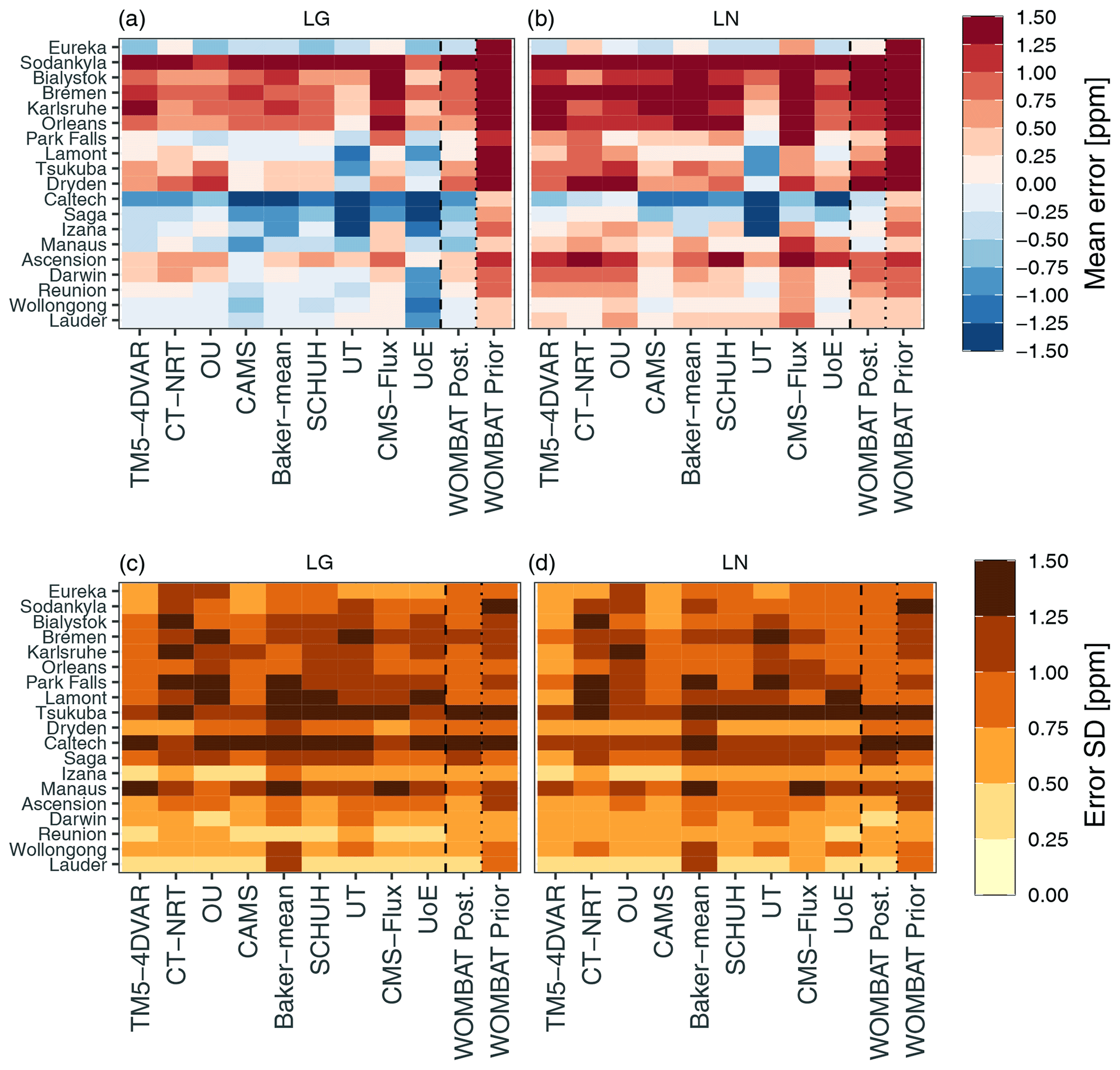
Figure 5Mean (a, b) and standard deviation (c, d) of the errors across TCCON stations for each MIP participant (refer to Crowell et al., 2019, for details) and WOMBAT's prior and posterior mean predicted values. The error statistics for inversions using LG data are shown in (a, c), while those for LN data are shown in (b, d). This figure reproduces and extends Fig. 8 of Crowell et al. (2019) with similar (but not identical) colour gradients.
Table 4Mean-squared error (in ppm2) averaged across TCCON stations, for each MIP participant, and for WOMBAT's prior and posterior mean predicted values (refer to Crowell et al., 2019, for participant details).
5.2.3 The inferred parameters
One of the key features of WOMBAT is the use of a parameter prior distribution in the hierarchical Bayesian model, which applies to both the parameters governing the flux scaling factors and to the parameters governing the model–data discrepancy and measurement error processes. Figure 6 shows the estimated posterior means and 95 % credible intervals for the autoregressive parameters κ (Fig. 6a) and the innovation precisions τw (Fig. 6b) for the 11 land regions and for inversions using LG and LN data. The inferred parameters are relatively consistent across the LG and LN modes, with the exception of TransCom3 region 02 (North American Temperate). Most regions have a posterior mean for κj that is approximately between 0.25 and 0.75, reflective of moderate autocorrelation in the scaling factors. The exception is TransCom3 region 03, for which the scaling factors are estimated to be highly autocorrelated a priori. The innovation precisions, τw, have posterior means that lie approximately between 1 and 10 for most regions.
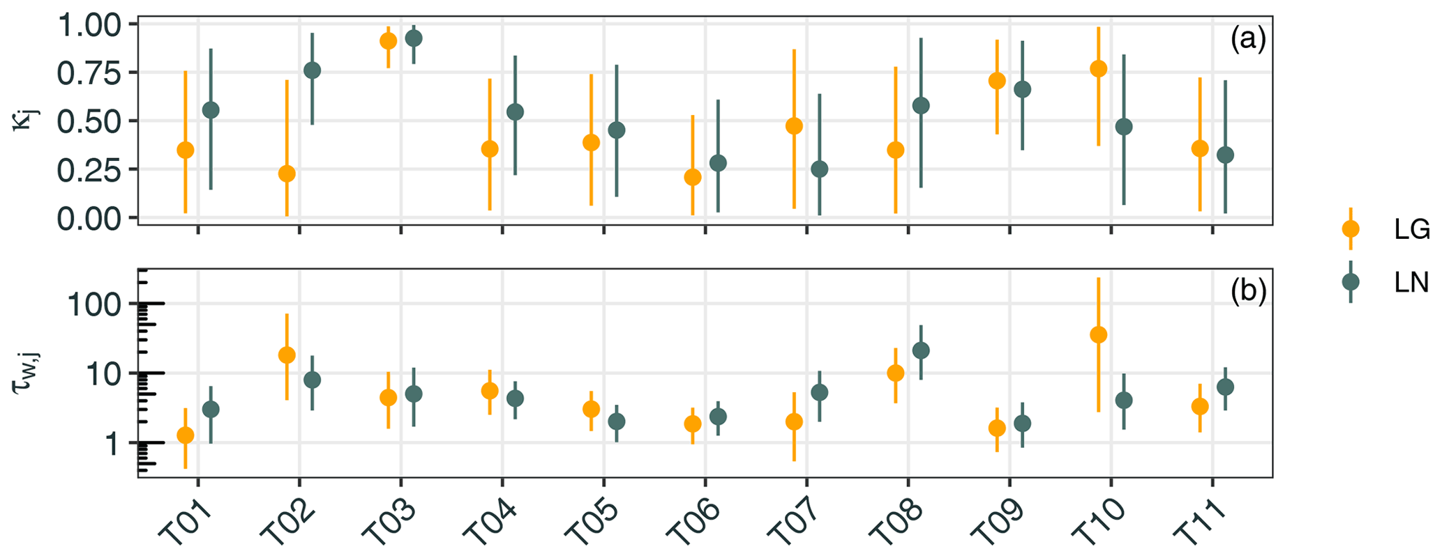
Figure 6Posterior means and 95 % credible intervals for κ (a) and τw (b, shown using a log scale), for the 11 land regions: TransCom3 region 01 (T01) to TransCom3 region 11 (T11). Estimates are shown for inversions using LG data (yellow) and LN data (dark green).
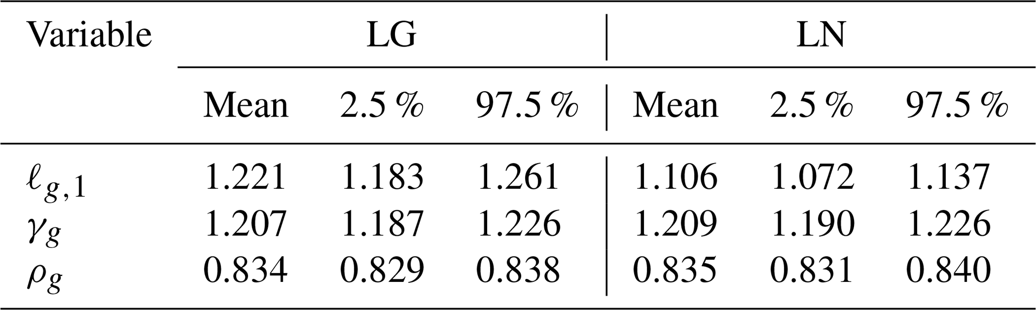
The parameters governing the model–data discrepancy and measurement error processes are ρg, ℓg,1, and γg, for . Table 5 gives the posterior means, 2.5 % quantiles, and 97.5 % quantiles for these parameters. Recall that the LG and LN parameters are derived from different inversions; that is, they are not two groups in the same inversion. Nonetheless, the inferred parameters are similar between the inversions, which is reassuring. The values for γg are indicative of a 21 % variance inflation needed for both instrument modes. The length scales, ℓg, are 1.2 min for the LG data and 1.1 min for the LN data, which corresponds to around 700 to 800 km on the ground. Finally, the estimated values of ρg are around 0.835, indicating that the majority of the combined model–data discrepancy and measurement error process should indeed be attributed to the correlated component, ξg, given in Eq. (9).
Table 5Posterior means, 2.5 % quantiles, and 97.5 % quantiles for the parameters ℓg,1, γg, and ρg for the inversions using LG and LN retrievals. Recall that the parameters associated with LG and LN are derived from different inversions and not from using the two retrieval groups in the same inversion.
5.3 Online bias correction
The OSSE-based sensitivity study in Sect. 5.1 demonstrated that WOMBAT is able to perform online bias correction with simulated data, where biases are estimated while doing flux inversion. This is different to the typical offline approach to bias correction, where retrieval biases are determined in a separate study (e.g. Wunch et al., 2011b). To comply with the MIP protocol, the online bias-correction functionality of WOMBAT was disabled in the study of Sect. 5.2, and the TCCON-based offline bias-corrected OCO-2 retrievals from the MIP were used. In order to investigate the prospect of online bias correction with real data, we repeat the inversions with online bias correction enabled, using OCO-2 10 s average retrievals both with and without the TCCON-based offline corrections.
In Fig. 7, we show the posterior densities of the WOMBAT-estimated bias-correction coefficients when using the retrievals without the offline correction. The posterior densities shown there are for inversions based on LG and LN retrievals, while the TCCON-based offline bias-correction coefficients are given by the blue vertical lines. The WOMBAT-estimated coefficients have the same sign and similar magnitudes to the offline corrections, suggesting that WOMBAT is picking up similar bias patterns while doing flux inversion. However, with the exception of the “dp” coefficient under the LN inversion, the offline values are outside the plausible ranges estimated by WOMBAT. For “co2_grad_del”, WOMBAT favours a smaller correction for both LG and LN, while for “logDWS” a larger correction is favoured. For “dp”, WOMBAT favours a smaller correction under the LG inversion.

Figure 7Posterior densities of bias-correction coefficients from inversions using OCO-2 retrievals without bias corrections applied (a, b, c) and those from inversions using retrievals corrected using the TCCON-based offline bias coefficients (d, e, f). Densities are shown for inversions based on LG and LN retrievals in yellow and dark green, respectively. The TCCON-based offline bias correction coefficients are shown as vertical blue lines for the panels in the top row. The vertical dashed grey lines in the bottom row mark zero, which is the value the coefficients would take if the data were unbiased.
We repeated the online bias-correction procedure using retrievals retaining the TCCON-based offline bias correction. In this setting, if the retrievals are unbiased, bias coefficients equal to zero should be inferred. The posterior densities of the estimated coefficients under this configuration are shown in the second row of Fig. 7. As expected, the magnitudes of the online-estimated coefficients are close to zero, although the credible intervals do not always include zero. Naïvely, one might expect that the coefficients would be approximately equal to the difference between the TCCON-based offline coefficients and the coefficients estimated by WOMBAT when using uncorrected data. For “dp” and “co2_grad_del”, the estimated coefficients indeed have the expected sign and the expected orders of magnitude. The inferred “logDWS” coefficients are surprising, however, with an opposite sign to what was expected for the LG inversion and smaller magnitudes for both the LG and LN inversions. This unexpected result is a reflection of the complex interplay and nonlinear relationships between the parameters and processes in a regularised flux-inversion model.
Overall, the online-estimated bias correction is practically, if not statistically, similar to the TCCON-based offline correction. One possible explanation for the difference between the WOMBAT and the TCCON-based estimates is that different data are used because WOMBAT does not use TCCON data for the correction. Moreover, it is likely that the true bias coefficients are spatio-temporally varying; if this is indeed the case, the estimated biases would be affected by the spatio-temporal locations of the retrievals used to estimate them. Another reason may be that, for simplicity, we have used only a few of the most important variables that are used for offline bias correction; a consideration of all the variables may lead to slightly different results. Despite this, our results show that online bias correction is possible and that further research into it as an attractive by-product of flux inversion is warranted.
Figure 8 gives annual and monthly fluxes estimated from the inversions using the online bias correction applied to the uncorrected retrievals. For comparison, the equivalent fluxes from Sect. 5.2.1 for the offline-corrected data and with the online bias correction disabled are also reported. The annual and monthly fluxes are similar between the offline-corrected and online-corrected inversions, with substantial overlap in the marginal posterior distributions for all time periods. This result gives further evidence that online bias correction is a viable alternative to offline correction (here based on TCCON data) when doing flux inversion.
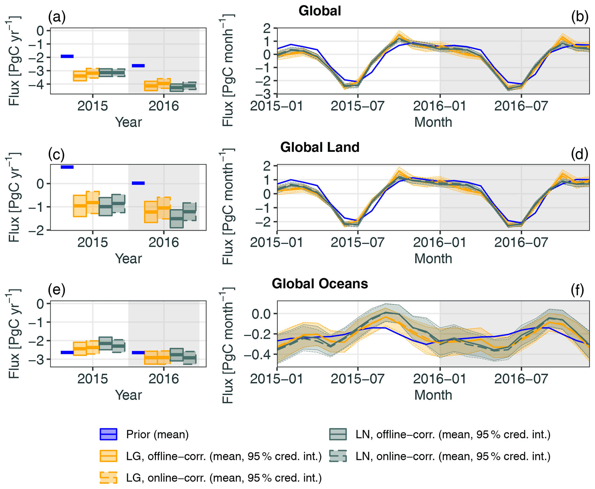
Figure 8Annual and monthly fluxes for WOMBAT inversions using TCCON-based offline bias-corrected retrievals (solid yellow lines for LG and dark green lines for LN; the fluxes are the same as in Figs. 4 and S4, respectively) and with online bias correction applied to the uncorrected retrievals (dashed lines). The prior-mean fluxes are shown in blue. Solid lines depict prior and posterior means, and shaded areas denote the 95 % credible intervals (cred. int.). Panels (a, b) depict global fluxes, (c, d) global land fluxes, and (e, f) global ocean fluxes.
The WOllongong Methodology for Bayesian Assimilation of Trace-gases (WOMBAT) extends the standard synthesis flux-inversion framework, which does not put prior distributions on all unknowns, to a framework based on a fully Bayesian hierarchical statistical model. It incorporates physically motivated flux basis functions and follows the standard Bayesian synthesis framework by using a CTM to compute the corresponding mole-fraction basis functions offline. The scaling factors for the basis functions are inferred from mole-fraction satellite data. WOMBAT incorporates a correlated-error term, estimates measurement biases and measurement error scaling factors online, estimates variances and length scales of flux scaling factors, and uses an MCMC scheme that allows uncertainty quantification through posterior distributions on all unknowns in the model. We have illustrated the importance of modelling correlation and bias within a flux-inversion system, and we have shown that WOMBAT produces global and regional flux estimates from OCO-2 data that are comparable to those from the MIP participants in Crowell et al. (2019). In particular, WOMBAT outperformed the other flux models in reproducing TCCON data when using the OCO-2 LG retrievals to obtain the fluxes, and it was competitive when using fluxes obtained from the OCO-2 LN retrievals. When the fossil-fuel fluxes are included, we estimate a global carbon source of 6.11±0.09 PgC yr−1 using the LG data and 6.17±0.07 PgC yr−1 using the LN data. These estimates corroborate those of the MIP within uncertainty.
This paper presents the general, underlying Bayesian hierarchical framework for WOMBAT v1.0, which will serve as a baseline for our flux inversions based on current and future versions of OCO-2 data. There are several potential extensions being considered; here we discuss three of the most pertinent ones. First, WOMBAT, like most other flux-inversion systems, currently operates using a single CTM. This is problematic from a statistical modelling point of view, as it does not allow one to attribute the correlated error either to the measurement error process or to the mole-fraction process. If more than one CTM is used, in principle one could statistically attribute at least part of the error to transport. This will not necessarily solve the problem though, since CTMs tend to share common features that induce similar correlations (e.g. due to unresolved sub-grid variation). A possible way forward is to take results from offline OSSEs to estimate and fix the parameters characterising the CTM error, and then to attribute any residual observed correlation to the retrieval process.
Second, WOMBAT extends a traditional state–space approach to flux inversion, which competes with adjoint-based approaches that allow for a much higher flux dimensionality. In the current version of WOMBAT, one should use the largest number of basis functions possible, given available hardware requirements, and find a compromise between the temporal and spatial resolution of the flux basis functions, such that the chosen resolution is as close as possible, or finer, than that at which the flux estimates need to be produced (in our case, this was the TransCom3-by-month level). At this chosen resolution we expect WOMBAT to perform well and give predictions that are valid within uncertainty: when one has broad spatial and temporal data coverage of the response functions, as in the case of OCO-2 and a TransCom3-by-month flux resolution, Bayesian synthesis can be expected to be reasonably robust to dimension-reduction error. Further, the WOMBAT posterior distributions over the fluxes are non-Gaussian and can accommodate skewness and long tails; this added flexibility mitigates the risk of under-fitting. Moreover, one may introduce additional scaling factors and corresponding basis functions in small “regions of interest”, where the fine-scale fluxes are an inferential target, and this is something we are doing in a follow-up iteration of WOMBAT. However, it would be desirable to have global inversions yield valid inferences at fine spatio-temporal scales globally. Moving forward, WOMBAT will therefore seek to introduce higher dimensionality by using flux basis functions that are at a finer scale than the TransCom3-by-month spatio-temporal basis functions that we have used here or a fine-scale variation term in the flux process model that can be used to absorb variation in the flux that cannot be explained by the basis functions.
Finally, WOMBAT currently only considers along-track correlations when modelling the correlation-error term, ξg. However, the general framework we have proposed, based on a sparse-precision matrix approximation, can be extended to model full space–time correlations. Dedicated investigations will be required to assess the feasibility of the implementation and the impact it will have on flux estimates.
As mentioned in Sect. 2.5, WOMBAT makes inference on the fluxes and the other parameters in the model using a Gibbs sampler, wherein samples of subsets of the parameters are iteratively drawn from their full conditional distributions (e.g. Tierney, 1994). Recall that the target distribution is , as shown in Eq. (10).
The Gibbs sampler in WOMBAT is as follows. Given the ith sample, {α[i], β[i], κ[i], , , the (i+1)th sample is generated sequentially in the following manner.
-
Sample α[i+1] and β[i+1] jointly from
. -
Sample κ[i+1] from .
-
Sample from .
-
Sample from .
In Appendices A1–A4, we give the details for Steps (1)–(4). In deriving the conditional distributions, we often make use of the Sherman–Morrison–Woodbury matrix identity and a matrix-determinant lemma (e.g. Henderson and Searle, 1981). The former identity states that,for conformable matrices A, U, C, and V,
whenever the required inverses exist, while the latter lemma states that
A1 Sampling α and β
Let , , and . Then
The log of this quantity is quadratic in x, and therefore the full conditional distribution of x is a multivariate Gaussian distribution:
where
and
As described in Sect. 3, Σϵ is diagonal and under Markov assumptions Σξ has a sparse inverse. These properties allow us to efficiently compute the required mean and covariance matrix through use of the Sherman–Morrison–Woodbury matrix identity. Once these are computed, sampling from Eq. (A1) is straightforward.
A2 Sampling κ
The full conditional distribution of κ is
where, recalling Sect. 2.4, p(κ) is a product of beta density functions. Since each κj and τw,j is associated with a spatial region, we also partition α by spatial region. That is, we define , where , . For , the rt-dimensional vector αj can therefore be associated with , and a rt×rt sub-block of the matrix , which we denote as . Under the autoregressive model in Sect. 2.4, , where
Since the flux scaling factors in each spatial region are treated as independent a priori, Eq. (A2) may be written as
where
To generate samples from Eq. (A2), we therefore successively sample κj, from its full conditional distribution (Eq. A3). Equation (A3) does not correspond to any standard distribution, and thus we use slice sampling (Neal, 2003) to sample from it.
A3 Sampling τw
Similar to κ, the conditional distribution of τw factorises across spatial regions, and it is therefore given by
where
The density function in Eq. (A4) is a gamma density function,
where and . Therefore, we sample from the full conditional distribution of τw by successively sampling τw,j, for directly from Eq. (A5).
A4 Sampling θξ,ϵ
Since we assume that the parameters governing the correlated and uncorrelated error terms are data-group specific, the full conditional distribution of θξ,ϵ is
where ; is the joint prior over and γg, and
The matrix operations in Eq. (A7) may be computed efficiently using the matrix identities given at the start of this appendix. Since Eq. (A7) does not correspond to any standard distribution, we use slice sampling to sample from it for .
The retrieval algorithm used for OCO-2 takes spectral data as input and returns CO2 mole fractions on 20 vertical levels as output via an optimisation procedure. The CO2 mole fractions at these 20 vertical levels are subsequently used to compute a column-averaged CO2 that we associate with a single retrieval. For the ith retrieval, we denote the vector of retrieved mole fractions as . Following the argument given by Rodgers and Connor (2003) and Connor et al. (2008), the retrieved mole fractions are given by
where is the vector of prior-mean mole fractions used by the retrieval algorithm, specific to the ith retrieval (these are unrelated to the prior mean of the mole-fraction field used in our inversion, ); Ai is the “averaging kernel matrix”; is the true mole fraction at the 20 vertical levels for the retrieval at geopotential heights hi,k, ; and is a vector of measurement errors (which may also include systematic biases and errors induced by nonlinearity in the inversion process). The column-averaged retrieval is then
where are quadrature weights used to estimate the column average, and is the retrieval prior mean column-averaged CO2. Define , where
and denotes the kth element of . The vector ai is the “averaging kernel vector” of the ith retrieval, which is available in the official releases of the OCO-2 data. It follows that the observation operator in Eq. (7) is defined as follows:
Note that we do not explicitly account for the error term in our definition for . This is because it will be absorbed by the error terms we use in the data model (Eq. 8).
The averaging-kernel vector elements {ai,k} are ideally close in value to 1. They reflect the fact that the retrieval is not equally sensitive to the mole fractions at all the vertical levels. At levels where there is less sensitivity (i.e. values <1), the retrieval prior-mean mole fraction will be assigned greater weight when producing the column-average CO2 estimate (Rodgers, 2000).
The code associated with this article is available at https://doi.org/10.5281/zenodo.4886771 (Bertolacci et al., 2021a). This code repository includes scripts for reproducing the entire analysis in this paper, which can be applied to a variety of inverse modelling problems. Re-running the entire analysis is computationally expensive due to the need to simulate atmospheric transport under various perturbations. To help with this, we provide these outputs as a separate download at https://doi.org/10.5281/zenodo.4887043 (Bertolacci et al., 2021b). These allow the inversions to be done and for results to be generated without the need to run the atmospheric transport model. Please see README.md in the code repository for more details.
The supplement related to this article is available online at: https://doi.org/10.5194/gmd-15-45-2022-supplement.
AZM, MB, and NC designed and wrote the study. JF, AS, MR, and YC contributed to the design and implementation of the GEOS-Chem model simulations. MB and AZM designed and implemented the MCMC algorithm and conducted the analyses.
The contact author has declared that neither they nor their co-authors have any competing interests.
Publisher’s note: Copernicus Publications remains neutral with regard to jurisdictional claims in published maps and institutional affiliations.
This project was largely supported by the Australian Research Council (ARC) Discovery Project (DP) DP190100180. Andrew Zammit-Mangion's research was also supported by an ARC Discovery Early Career Research Award (DECRA) DE180100203. Noel Cressie's research was also supported by ARC DP150104576. Noel Cressie's and Andrew Zammit-Mangion's research was also supported by NASA ROSES grant 17-OCO2-17-0012. Jenny Fisher was supported by ARC DP160101598. Ann Stavert and Matthew Rigby were supported by the UK Natural Environment Research Council (grant no. NE/K002236/1). The TCCON data were obtained from the TCCON Data Archive hosted by CaltechDATA at https://tccondata.org/ (last access: 16 November 2021). The authors would also like to thank David Baker for generating the OCO-2 10 s average retrievals and Beata Bukosa, Nicholas Deutscher, Anita Ganesan, Peter Rayner, Andrew Schuh, and members of the OCO-2 Flux Team for invaluable feedback on this research. This work was supported by resources provided by the Pawsey Supercomputing Centre with funding from the Australian Government and the Government of Western Australia. The work was also supported by the NCI National Facility systems at the Australian National University through the National Computational Merit Allocation Scheme supported by the Australian Government.
This research has been supported by the Australian Research Council (grant nos. DP190100180, DE180100203, DP160101598, and DP150104576), the National Aeronautics and Space Administration (grant no. 17-OCO2-17-0012), the Natural Environment Research Council (grant no. NE/K002236/1), and the Australian Government and the Government of Western Australia (National Computational Merit Allocation Scheme project code m19 and resources provided by the Pawsey Supercomputing Centre).
This paper was edited by Sergey Gromov and reviewed by Scot Miller and one anonymous referee.
Abadi, M., Agarwal, A., Barham, P., Brevdo, E., Chen, Z., Citro, C., Corrado, G. S., Davis, A., Dean, J., Devin, M., Ghemawat, S., Goodfellow, I., Harp, A., Irving, G., Isard, M., Jia, Y., Jozefowicz, R., Kaiser, L., Kudlur, M., Levenberg, J., Mane, D., Monga, R., Moore, S., Murray, D., Olah, C., Schuster, M., Shlens, J., Steiner, B., Sutskever, I., Talwar, K., Tucker, P., Vanhoucke, V., Vasudevan, V., Viegas, F., Vinyals, O., Warden, P., Wattenberg, M., Wicke, M., Yu, Y., and Zheng, X.: TensorFlow: Large-Scale Machine Learning on Heterogeneous Distributed Systems, arXiv [preprint], 1603.04467, 16 March 2016. a
Baker, D. F., Doney, S. C., and Schimel, D. S.: Variational data assimilation for atmospheric CO2, Tellus B, 58, 359–365, https://doi.org/10.1111/j.1600-0889.2006.00218.x, 2006. a
Basu, S., Guerlet, S., Butz, A., Houweling, S., Hasekamp, O., Aben, I., Krummel, P., Steele, P., Langenfelds, R., Torn, M., Biraud, S., Stephens, B., Andrews, A., and Worthy, D.: Global CO2 fluxes estimated from GOSAT retrievals of total column CO2, Atmos. Chem. Phys., 13, 8695–8717, https://doi.org/10.5194/acp-13-8695-2013, 2013. a, b, c, d, e, f
Basu, S., Baker, D. F., Chevallier, F., Patra, P. K., Liu, J., and Miller, J. B.: The impact of transport model differences on CO2 surface flux estimates from OCO-2 retrievals of column average CO2, Atmos. Chem. Phys., 18, 7189–7215, https://doi.org/10.5194/acp-18-7189-2018, 2018. a, b, c
Bertolacci, M., Zammit-Mangion, A., Cao, Y., Fisher, J., and Stavert, A.: WOMBAT: A fully Bayesian global flux-inversion framework, version 1, Zenodo [code], https://doi.org/10.5281/zenodo.4886771, 2021a. a
Bertolacci, M., Fisher, J., Cao, Y., Stavert, A., and Rigby, M.: WOMBAT: A fully Bayesian global flux-inversion framework, version 1 (intermediate files), Zenodo [data set], https://doi.org/10.5281/zenodo.4887043, 2021b. a
Bey, I., Jacob, D. J., Yantosca, R. M., Logan, J. A., Field, B. D., Fiore, A. M., Li, Q., Liu, H. Y., Mickley, L. J., and Schultz, M. G.: Global Modeling of Tropospheric Chemistry with Assimilated Meteorology: Model Description and Evaluation, J. Geophys. Res., 106, 23073–23095, https://doi.org/10.1029/2001JD000807, 2001. a
Blumenstock, T., Hase, F., Schneider, M., García, O. E., and Sepúlveda, E.: TCCON data from Izaña (ES), Release GGG2014.R0, CaltechDATA [data set], https://doi.org/10.14291/tccon.ggg2014.izana01.R0/1149295, 2014. a
Brynjarsdóttir, J. and O'Hagan, A.: Learning about physical parameters: the importance of model discrepancy, Inverse Problems, 30, 114007, https://doi.org/10.1088/0266-5611/30/11/114007, 2014. a
Bukosa, B., Deutscher, N. M., Fisher, J. A., Kubistin, D., Paton-Walsh, C., and Griffith, D. W. T.: Simultaneous shipborne measurements of CO2, CH4 and CO and their application to improving greenhouse-gas flux estimates in Australia, Atmos. Chem. Phys., 19, 7055–7072, https://doi.org/10.5194/acp-19-7055-2019, 2019. a, b
Burrows, J. P., Hölzle, E., Goede, A. P. H., Visser, H., and Fricke, W.: SCIAMACHY–Scanning Imaging Absorption Spectrometer for Atmospheric Chartography, Acta Astronaut., 35, 445–451, https://doi.org/10.1016/0094-5765(94)00278-T, 1995. a
Chevallier, F.: Impact of Correlated Observation Errors on Inverted CO2 Surface Fluxes from OCO Measurements, Geophys. Res. Lett., 34, L24804, https://doi.org/10.1029/2007GL030463, 2007. a, b, c
Chevallier, F., Fisher, M., Peylin, P., Serrar, S., Bousquet, P., Bréon, F.-M., Chédin, A., and Ciais, P.: Inferring CO2 sources and sinks from satellite observations: Method and application to TOVS data, J. Geophys. Res., 110, D24309, https://doi.org/10.1029/2005JD006390, 2005. a, b
Chevallier, F., Bréon, F.-M., and Rayner, P. J.: Contribution of the Orbiting Carbon Observatory to the estimation of CO2 sources and sinks: Theoretical study in a variational data assimilation framework, J. Geophys. Res., 112, D09307, https://doi.org/10.1029/2006JD007375, 2007. a, b
Ciais, P., Rayner, P., Chevallier, F., Bousquet, P., Logan, M., Peylin, P., and Ramonet, M.: Atmospheric inversions for estimating CO2 fluxes: methods and perspectives, Climatic Change, 103, 69–92, https://doi.org/10.1007/s10584-010-9909-3, 2010. a, b
Connor, B. J., Boesch, H., Toon, G., Sen, B., Miller, C., and Crisp, D.: Orbiting Carbon Observatory: Inverse method and prospective error analysis, J. Geophys. Res., 113, D05305, https://doi.org/10.1029/2006JD008336, 2008. a
Crowell, S., Baker, D., Schuh, A., Basu, S., Jacobson, A. R., Chevallier, F., Liu, J., Deng, F., Feng, L., McKain, K., Chatterjee, A., Miller, J. B., Stephens, B. B., Eldering, A., Crisp, D., Schimel, D., Nassar, R., O'Dell, C. W., Oda, T., Sweeney, C., Palmer, P. I., and Jones, D. B. A.: The 2015–2016 carbon cycle as seen from OCO-2 and the global in situ network, Atmos. Chem. Phys., 19, 9797–9831, https://doi.org/10.5194/acp-19-9797-2019, 2019. a, b, c, d, e, f, g, h, i, j, k, l, m, n, o, p, q, r, s
Dahlén, U., Lindström, J., and Scholze, M.: Spatiotemporal Reconstructions of Global CO2-Fluxes Using Gaussian Markov Random Fields, Environmetrics, 31, e2610, https://doi.org/10.1002/env.2610, 2020. a
Darmenov, A. and da Silva, A.: The Quick Fire Emissions Dataset (QFED): Documentation of versions 2.1, 2.2 and 2.4, NASA Technical Report Series on Global Modeling and Data Assimilation, Tech. Rep. NASA/TM-2015-104606, available at: http://gmao.gsfc.nasa.gov/pubs/docs/Darmenov796.pdf (last access: 16 November 2021), 2015. a, b
Datta, A., Banerjee, S., Finley, A. O., and Gelfand, A. E.: Hierarchical nearest-neighbor Gaussian process models for large geostatistical datasets, J. Am. Stat. Assoc., 111, 800–812, https://doi.org/10.1080/01621459.2015.1044091, 2016. a
De Mazière, M., Sha, M. K., Desmet, F., Hermans, C., Scolas, F., Kumps, N., Metzger, J.-M., Duflot, V., and Cammas, J.-P.: TCCON data from Réunion Island (RE), Release GGG2014.R0, CaltechDATA [data set], https://doi.org/10.14291/tccon.ggg2014.reunion01.R0/1149288, 2014. a
Deng, F., Jones, D. B., O'Dell, C. W., Nassar, R., and Parazoo, N. C.: Combining GOSAT XCO2 observations over land and ocean to improve regional CO2 flux estimates, J. Geophys. Res.-Atmos., 121, 1896–1913, https://doi.org/10.1002/2015JD024157, 2016. a
Deutscher, N. M., Notholt, J., Messerschmidt, J., Weinzierl, C., Warneke, T., Petri, C., and Grupe, P.: TCCON data from Bialystok (PL), Release GGG2014.R1, CaltechDATA [data set], https://doi.org/10.14291/tccon.ggg2014.bialystok01.R1/1183984, 2015. a
Dlugokencky, E. and Tans, P.: Trends in atmospheric carbon dioxide, National Oceanic & Atmospheric Administration, Earth System Research Laboratory (NOAA/ESRL), available at: http://www.esrl.noaa.gov/gmd/ccgg/trends, last access: 11 December 2020. a
Dubey, M. K., Henderson, B. G., Green, D., Butterfield, Z. T., Keppel-Aleks, G., Allen, N. T., Blavier, J.-F., Roehl, C. M., Wunch, D., and Lindenmaier, R.: TCCON data from Manaus (BR), Release GGG2014.R0, CaltechDATA [data set], https://doi.org/10.14291/tccon.ggg2014.manaus01.R0/1149274, 2014. a
Edenhofer, O., R., Pichs-Madruga, Y., Sokona, E., Farahani, S., Kadner, K., Seyboth, A., Adler, I., Baum, S., Brunner, P., Eickemeier, B., Kriemann, J., Savolainen, S., Schlömer, C., von Stechow, T., Zwickel, and Minx, J.: IPCC, 2014: Summary for Policymakers, in: Climate Change 2014: Mitigation of Climate Change. Contribution of Working Group III to the Fifth Assessment Report of the Intergovernmental Panel on Climate Change, Cambridge University Press, Cambridge, UK, 2014. a
Eldering, A., O'Dell, C. W., Wennberg, P. O., Crisp, D., Gunson, M. R., Viatte, C., Avis, C., Braverman, A., Castano, R., Chang, A., Chapsky, L., Cheng, C., Connor, B., Dang, L., Doran, G., Fisher, B., Frankenberg, C., Fu, D., Granat, R., Hobbs, J., Lee, R. A. M., Mandrake, L., McDuffie, J., Miller, C. E., Myers, V., Natraj, V., O'Brien, D., Osterman, G. B., Oyafuso, F., Payne, V. H., Pollock, H. R., Polonsky, I., Roehl, C. M., Rosenberg, R., Schwandner, F., Smyth, M., Tang, V., Taylor, T. E., To, C., Wunch, D., and Yoshimizu, J.: The Orbiting Carbon Observatory-2: first 18 months of science data products, Atmos. Meas. Tech., 10, 549–563, https://doi.org/10.5194/amt-10-549-2017, 2017. a, b
Eldering, A., Taylor, T. E., O'Dell, C. W., and Pavlick, R.: The OCO-3 mission: measurement objectives and expected performance based on 1 year of simulated data, Atmos. Meas. Tech., 12, 2341–2370, https://doi.org/10.5194/amt-12-2341-2019, 2019. a
Engelen, R. J., Denning, A. S., and Gurney, K. R.: On error estimation in atmospheric CO2 inversions, J. Geophys. Res., 107, 4635, https://doi.org/10.1029/2002JD002195, 2002. a
Enting, I. G.: Inverse Problems in Atmospheric Constituent Transport, Cambridge University Press, Cambridge, UK, https://doi.org/10.1017/CBO9780511535741, 2002. a, b, c, d, e, f
Fan, S., Gloor, M., Mahlman, J., Pacala, S., Sarmiento, J., Takahashi, T., and Tans, P.: A large terrestrial carbon sink in North America implied by atmospheric and oceanic carbon dioxide data and models, Science, 282, 442–446, 1998. a
Feist, D. G., Arnold, S. G., John, N., and Geibel, M. C.: TCCON data from Ascension Island (SH), Release GGG2014.R0, CaltechDATA [data set], https://doi.org/10.14291/tccon.ggg2014.ascension01.r0/1149285, 2014. a
Feng, L., Palmer, P. I., Bösch, H., and Dance, S.: Estimating surface CO2 fluxes from space-borne CO2 dry air mole fraction observations using an ensemble Kalman Filter, Atmos. Chem. Phys., 9, 2619–2633, https://doi.org/10.5194/acp-9-2619-2009, 2009. a
Feng, S., Lauvaux, T., Keller, K., Davis, K. J., Rayner, P., Oda, T., and Gurney, K. R.: A road map for improving the treatment of uncertainties in high-resolution regional carbon flux inverse estimates, Geophys. Res. Lett., 46, 13461–13469, https://doi.org/10.1029/2019GL082987, 2019. a
Ganesan, A. L., Rigby, M., Zammit-Mangion, A., Manning, A. J., Prinn, R. G., Fraser, P. J., Harth, C. M., Kim, K.-R., Krummel, P. B., Li, S., Mühle, J., O'Doherty, S. J., Park, S., Salameh, P. K., Steele, L. P., and Weiss, R. F.: Characterization of uncertainties in atmospheric trace gas inversions using hierarchical Bayesian methods, Atmos. Chem. Phys., 14, 3855–3864, https://doi.org/10.5194/acp-14-3855-2014, 2014. a, b, c
Giglio, L., Randerson, J. T., and van der Werf, G. R.: Analysis of daily, monthly, and annual burned area using the fourth-generation global fire emissions database (GFED4), J. Geophys. Res.-Biogeo., 118, 317–328, https://doi.org/10.1002/jgrg.20042, 2013. a, b
Gneiting, T. and Raftery, A. E.: Strictly Proper Scoring Rules, Prediction, and Estimation, J. Am. Stat. Assoc., 102, 359–378, https://doi.org/10.1198/016214506000001437, 2007. a
Griffith, D. W., Deutscher, N. M., Velazco, V. A., Wennberg, P. O., Yavin, Y., Keppel-Aleks, G., Washenfelder, R. A., Toon, G. C., Blavier, J.-F., Paton-Walsh, C., Jones, N. B., Kettlewell, G. C., Connor, B. J., Macatangay, R. C., Roehl, C., Ryczek, M., Glowacki, J., Culgan, T., and Bryant, G. W.: TCCON data from Darwin (AU), Release GGG2014.R0, CaltechDATA [data set], https://doi.org/10.14291/tccon.ggg2014.darwin01.R0/1149290, 2014a. a
Griffith, D. W., Velazco, V. A., Deutscher, N. M., Paton-Walsh, C., Jones, N. B., Wilson, S. R., Macatangay, R. C., Kettlewell, G. C., Buchholz, R. R., and Riggenbach, M. O.: TCCON data from Wollongong (AU), Release GGG2014.R0, CaltechDATA [data set], https://doi.org/10.14291/tccon.ggg2014.wollongong01.R0/1149291, 2014b. a
Gurney, K. R., Law, R. M., Denning, A. S., Rayner, P. J., Baker, D., Bousquet, P., Bruhwiler, L., Chen, Y.-H., Ciais, P., Fan, S., Fung, I. Y., Gloor, M., Heimann, M., Higuchi, K., John, J., Maki, T., Maksyutov, S., Masarie, K., Peylin, P., Prather, M., Pak, B. C., Randerson, J., Sarmiento, J., Taguchi, S., Takahashi, T., and Yuen, C.-W.: Towards robust regional estimates of CO2 sources and sinks using atmospheric transport models, Nature, 415, 626–630, https://doi.org/10.1038/415626a, 2002. a, b
Hase, F., Blumenstock, T., Dohe, S., Groß, J., and Kiel, M.: TCCON data from Karlsruhe (DE), Release GGG2014.R1, CaltechDATA [data set], https://doi.org/10.14291/tccon.ggg2014.karlsruhe01.R1/1182416, 2015. a
Henderson, H. V. and Searle, S. R.: On deriving the inverse of a sum of matrices, Siam Rev., 23, 53–60, 1981. a, b
Houweling, S., Aben, I., Breon, F.-M., Chevallier, F., Deutscher, N., Engelen, R., Gerbig, C., Griffith, D., Hungershoefer, K., Macatangay, R., Marshall, J., Notholt, J., Peters, W., and Serrar, S.: The importance of transport model uncertainties for the estimation of CO2 sources and sinks using satellite measurements, Atmos. Chem. Phys., 10, 9981–9992, https://doi.org/10.5194/acp-10-9981-2010, 2010. a
Huntzinger, D., Michalak, A., Schwalm, C., Ciais, P., King, A., Fang, Y., Schaefer, K., Wei, Y., Cook, R., Fisher, J., Hayes, D., Huang, M., Ito, A., Jain, A., Lei, H., Lu, C., Maignan, F., Mao, J., Parazoo, N., Peng, S., Poulter, B., Ricciuto, D., Shi, X., Tian, H., Wang, W., Zeng, N., and Zhao, F.: Uncertainty in the response of terrestrial carbon sink to environmental drivers undermines carbon-climate feedback predictions, Scientific Reports, 7, 1–8, 2017. a
Iraci, L. T., Podolske, J. R., Hillyard, P. W., Roehl, C., Wennberg, P. O., Blavier, J.-F., Landeros, J., Allen, N., Wunch, D., Zavaleta, J., Quigley, E., Osterman, G. B., Albertson, R., Dunwoody, K., and Boyden, H.: TCCON data from Edwards (US), Release GGG2014.R1, CaltechDATA [data set], https://doi.org/10.14291/tccon.ggg2014.edwards01.r1/1255068, 2016. a
Jacobson, A. R., Schuldt, K. N., Miller, J. B., Oda, T., Tans, P., Arlyn Andrews, Mund, J., Ott, L., Collatz, G. J., Aalto, T., Afshar, S., Aikin, K., Aoki, S., Apadula, F., Baier, B., Bergamaschi, P., Beyersdorf, A., Biraud, S. C., Bollenbacher, A., Bowling, D., Brailsford, G., Abshire, J. B., Chen, G., Chen, H., Chmura, L., Climadat, S., Colomb, A., Conil, S., Cox, A., Cristofanelli, P., Cuevas, E., Curcoll, R., Sloop, C. D., Davis, K., Wekker, S. D., Delmotte, M., DiGangi, J. P., Dlugokencky, E., Ehleringer, J., Elkins, J. W., Emmenegger, L., Fischer, M. L., Forster, G., Frumau, A., Galkowski, M., Gatti, L. V., Gloor, E., Griffis, T., Hammer, S., Haszpra, L., Hatakka, J., Heliasz, M., Hensen, A., Hermanssen, O., Hintsa, E., Holst, J., Jaffe, D., Karion, A., Kawa, S. R., Keeling, R., Keronen, P., Kolari, P., Kominkova, K., Kort, E., Krummel, P., Kubistin, D., Labuschagne, C., Langenfelds, R., Laurent, O., Laurila, T., Lauvaux, T., Law, B., Lee, J., Lehner, I., Leuenberger, M., Levin, I., Levula, J., Lin, J., Lindauer, M., Loh, Z., Lopez, M., Myhre, C. L., Machida, T., Mammarella, I., Manca, G., Manning, A., Manning, A., Marek, M. V., Marklund, P., Martin, M. Y., Matsueda, H., McKain, K., Meijer, H., Meinhardt, F., Miles, N., Miller, C. E., Mölder, M., Montzka, S., Moore, F., Morgui, J.-A., Morimoto, S., Munger, B., Necki, J., Newman, S., Nichol, S., Niwa, Y., O'Doherty, S., Ottosson-Löfvenius, M., Paplawsky, B., Peischl, J., Peltola, O., Pichon, J.-M., Piper, S., Plass-Dölmer, C., Ramonet, M., Reyes-Sanchez, E., Richardson, S., Riris, H., Ryerson, T., Saito, K., Sargent, M., Sasakawa, M., Sawa, Y., Say, D., Scheeren, B., Schmidt, M., Schmidt, A., Schumacher, M., Shepson, P., Shook, M., Stanley, K., Steinbacher, M., Stephens, B., Sweeney, C., Thoning, K., Torn, M., Turnbull, J., Tørseth, K., Bulk, P. V. D., van der Laan-Luijkx, I. T., Dinther, D. V., Vermeulen, A., Viner, B., Vitkova, G., Walker, S., Weyrauch, D., Wofsy, S., Worthy, D., Young, D., and Zimnoch, M.: CarbonTracker CT2019, Model, NOAA Earth System Research Laboratory, Global Monitoring Division, https://doi.org/10.25925/39m3-6069, available at: https://www.esrl.noaa.gov/gmd/ccgg/carbontracker/CT2019_doc.php (last access: 16 November 2021), 2020. a, b, c
Kaminski, T., Rayner, P. J., Heimann, M., and Enting, I. G.: On aggregation errors in atmospheric transport inversions, J. Geophys. Res., 106, 4703–4715, https://doi.org/10.1029/2000JD900581, 2001. a
Kawakami, S., Ohyama, H., Arai, K., Okumura, H., Taura, C., Fukamachi, T., and Sakashita, M.: TCCON data from Saga (JP), Release GGG2014.R0, CaltechDATA [data set], https://doi.org/10.14291/tccon.ggg2014.saga01.R0/1149283, 2014. a
Keller, C. A., Long, M. S., Yantosca, R. M., Da Silva, A. M., Pawson, S., and Jacob, D. J.: HEMCO v1.0: a versatile, ESMF-compliant component for calculating emissions in atmospheric models, Geosci. Model Dev., 7, 1409–1417, https://doi.org/10.5194/gmd-7-1409-2014, 2014. a
Kivi, R., Heikkinen, P., and Kyrö, E.: TCCON data from Sodankylä (FI), Release GGG2014.R0, CaltechDATA [data set], https://doi.org/10.14291/tccon.ggg2014.sodankyla01.R0/1149280, 2014. a
Kuze, A., Suto, H., Nakajima, M., and Hamazaki, T.: Thermal and near Infrared Sensor for Carbon Observation Fourier-Transform Spectrometer on the Greenhouse Gases Observing Satellite for Greenhouse Gases Monitoring, Appl. Optics, 48, 6716–6733, https://doi.org/10.1364/AO.48.006716, 2009. a
Lauvaux, T., Díaz-Isaac, L. I., Bocquet, M., and Bousserez, N.: Diagnosing spatial error structures in CO2 mole fractions and XCO2 column mole fractions from atmospheric transport, Atmos. Chem. Phys., 19, 12007–12024, https://doi.org/10.5194/acp-19-12007-2019, 2019. a, b
Liu, J., Bowman, K. W., Lee, M., Henze, D. K., Bousserez, N., Brix, H., James Collatz, G., Menemenlis, D., Ott, L., Pawson, S., Jones, D., and Nassar, R.: Carbon monitoring system flux estimation and attribution: impact of ACOS-GOSAT X sampling on the inference of terrestrial biospheric sources and sinks, Tellus B, 66, 22486, https://doi.org/10.3402/tellusb.v66.22486, 2014. a
Masarie, K. A., Peters, W., Jacobson, A. R., and Tans, P. P.: ObsPack: a framework for the preparation, delivery, and attribution of atmospheric greenhouse gas measurements, Earth Syst. Sci. Data, 6, 375–384, https://doi.org/10.5194/essd-6-375-2014, 2014. a
McNorton, J. R., Bousserez, N., Agustí-Panareda, A., Balsamo, G., Choulga, M., Dawson, A., Engelen, R., Kipling, Z., and Lang, S.: Representing model uncertainty for global atmospheric CO2 flux inversions using ECMWF-IFS-46R1, Geosci. Model Dev., 13, 2297–2313, https://doi.org/10.5194/gmd-13-2297-2020, 2020. a, b
Michalak, A. M., Bruhwiler, L., and Tans, P. P.: A geostatistical approach to surface flux estimation of atmospheric trace gases, J. Geophys. Res., 109, D14109, https://doi.org/10.1029/2003JD004422, 2004. a, b
Michalak, A. M., Hirsch, A., Bruhwiler, L., Gurney, K. R., Peters, W., and Tans, P. P.: Maximum likelihood estimation of covariance parameters for Bayesian atmospheric trace gas surface flux inversions, J. Geophys. Res., 110, D24107, https://doi.org/10.1029/2005JD005970, 2005. a, b
Miller, S. M., Michalak, A. M., and Levi, P. J.: Atmospheric inverse modeling with known physical bounds: an example from trace gas emissions, Geosci. Model Dev., 7, 303–315, https://doi.org/10.5194/gmd-7-303-2014, 2014. a
Miller, S. M., Saibaba, A. K., Trudeau, M. E., Mountain, M. E., and Andrews, A. E.: Geostatistical inverse modeling with very large datasets: an example from the Orbiting Carbon Observatory 2 (OCO-2) satellite, Geosci. Model Dev., 13, 1771–1785, https://doi.org/10.5194/gmd-13-1771-2020, 2020. a
Morino, I., Matsuzaki, T., and Horikawa, M.: TCCON data from Tsukuba (JP), 125HR, Release GGG2014.R1, Version GGG2014.R1, CaltechDATA [Data set], https://doi.org/10.14291/tccon.ggg2014.tsukuba02.R1/1241486, 2016. a
Mukherjee, C., Kasibhatla, P. S., and West, M.: Bayesian statistical modeling of spatially correlated error structure in atmospheric tracer inverse analysis, Atmos. Chem. Phys., 11, 5365–5382, https://doi.org/10.5194/acp-11-5365-2011, 2011. a, b, c
Nassar, R., Jones, D. B. A., Suntharalingam, P., Chen, J. M., Andres, R. J., Wecht, K. J., Yantosca, R. M., Kulawik, S. S., Bowman, K. W., Worden, J. R., Machida, T., and Matsueda, H.: Modeling global atmospheric CO2 with improved emission inventories and CO2 production from the oxidation of other carbon species, Geosci. Model Dev., 3, 689-716, https://doi.org/10.5194/gmd-3-689-2010, 2010. a
Nassar, R., Napier-Linton, L., Gurney, K. R., Andres, R. J., Oda, T., Vogel, F. R., and Deng, F.: Improving the temporal and spatial distribution of CO2 emissions from global fossil fuel emission data sets, J. Geophys. Res.-Atmos., 118, 917–933, https://doi.org/10.1029/2012JD018196, 2013. a, b
Neal, R. M.: Slice sampling, Ann. Stat., 31, 705–741, https://doi.org/10.1214/aos/1056562461, 2003. a, b
Notholt, J., Petri, C., Warneke, T., Deutscher, N. M., Palm, M., Buschmann, M., Weinzierl, C., Macatangay, R. C., and Grupe, P.: TCCON data from Bremen (DE), Release GGG2014.R0, CaltechDATA [data set], https://doi.org/10.14291/tccon.ggg2014.bremen01.R0/1149275, 2014. a
Oda, T. and Maksyutov, S.: A very high-resolution (1 km × 1 km) global fossil fuel CO2 emission inventory derived using a point source database and satellite observations of nighttime lights, Atmos. Chem. Phys., 11, 543–556, https://doi.org/10.5194/acp-11-543-2011, 2011. a, b
Oda, T., Maksyutov, S., and Andres, R. J.: The Open-source Data Inventory for Anthropogenic CO2, version 2016 (ODIAC2016): a global monthly fossil fuel CO2 gridded emissions data product for tracer transport simulations and surface flux inversions, Earth Syst. Sci. Data, 10, 87–107, https://doi.org/10.5194/essd-10-87-2018, 2018. a, b
O'Dell, C. W., Connor, B., Bösch, H., O'Brien, D., Frankenberg, C., Castano, R., Christi, M., Eldering, D., Fisher, B., Gunson, M., McDuffie, J., Miller, C. E., Natraj, V., Oyafuso, F., Polonsky, I., Smyth, M., Taylor, T., Toon, G. C., Wennberg, P. O., and Wunch, D.: The ACOS CO2 retrieval algorithm – Part 1: Description and validation against synthetic observations, Atmos. Meas. Tech., 5, 99–121, https://doi.org/10.5194/amt-5-99-2012, 2012. a, b
O'Dell, C. W., Eldering, A., Wennberg, P. O., Crisp, D., Gunson, M. R., Fisher, B., Frankenberg, C., Kiel, M., Lindqvist, H., Mandrake, L., Merrelli, A., Natraj, V., Nelson, R. R., Osterman, G. B., Payne, V. H., Taylor, T. E., Wunch, D., Drouin, B. J., Oyafuso, F., Chang, A., McDuffie, J., Smyth, M., Baker, D. F., Basu, S., Chevallier, F., Crowell, S. M. R., Feng, L., Palmer, P. I., Dubey, M., García, O. E., Griffith, D. W. T., Hase, F., Iraci, L. T., Kivi, R., Morino, I., Notholt, J., Ohyama, H., Petri, C., Roehl, C. M., Sha, M. K., Strong, K., Sussmann, R., Te, Y., Uchino, O., and Velazco, V. A.: Improved retrievals of carbon dioxide from Orbiting Carbon Observatory-2 with the version 8 ACOS algorithm, Atmos. Meas. Tech., 11, 6539–6576, https://doi.org/10.5194/amt-11-6539-2018, 2018. a
Peters, G. P., Andrew, R. M., Boden, T., Canadell, J. G., Ciais, P., Le Quéré, C., Marland, G., Raupach, M. R., and Wilson, C.: The challenge to keep global warming below 2 ∘C, Nat. Clim. Change, 3, 4–6, https://doi.org/10.1038/nclimate1783, 2013. a
Peters, W., Miller, J., Whitaker, J., Denning, A., Hirsch, A., Krol, M., Zupanski, D., Bruhwiler, L., and Tans, P.: An ensemble data assimilation system to estimate CO2 surface fluxes from atmospheric trace gas observations, J. Geophys. Res., 110, D24304, https://doi.org/10.1029/2005JD006157, 2005. a, b
Philip, S., Johnson, M. S., Potter, C., Genovesse, V., Baker, D. F., Haynes, K. D., Henze, D. K., Liu, J., and Poulter, B.: Prior biosphere model impact on global terrestrial CO2 fluxes estimated from OCO-2 retrievals, Atmos. Chem. Phys., 19, 13267–13287, https://doi.org/10.5194/acp-19-13267-2019, 2019. a
Potter, C. S., Randerson, J. T., Field, C. B., Matson, P. A., Vitousek, P. M., Mooney, H. A., and Klooster, S. A.: Terrestrial ecosystem production: a process model based on global satellite and surface data, Global Biogeochem. Cy., 7, 811–841, https://doi.org/10.1029/93GB02725, 1993. a, b
R Core Team: R: A Language and Environment for Statistical Computing, R Foundation for Statistical Computing, Vienna, Austria, available at: https://www.R-project.org/ (last access: 16 November 2021), 2020. a
Rayner, P. and O'Brien, D.: The utility of remotely sensed CO2 concentration data in surface source inversions, Geophys. Res. Lett., 28, 175–178, https://doi.org/10.1029/2000GL011912, 2001. a
Rienecker, M. M., Suarez, M. J., Todling, R., Bacmeister, J., Takacs, L., Liu, H.-C., Gu, W., Sienkiewicz, M., Koster, R. D., Gelaro, R., Stajner, I., and Nielsen, J.: The GEOS-5 Data Assimilation System-Documentation of Versions 5.0.1, 5.1.0, and 5.2.0, NASA Tech. Rep. TM-2008-104606, 2008. a
Rodgers, C. D.: Inverse Methods for Atmospheric Sounding, World Scientific, Singapore, Singapore, https://doi.org/10.1142/3171, 2000. a, b
Rodgers, C. D. and Connor, B. J.: Intercomparison of Remote Sounding Instruments, J. Geophys. Res., 108, 4116, https://doi.org/10.1029/2002JD002299, 2003. a
Saeki, T., Maksyutov, S., Sasakawa, M., Machida, T., Arshinov, M., Tans, P., Conway, T. J., Saito, M., Valsala, V., Oda, T., Andres, R. J., and Belikov, D.: Carbon flux estimation for Siberia by inverse modeling constrained by aircraft and tower CO2 measurements, J. Geophys. Res.-Atmos., 118, 1100–1122, https://doi.org/10.1002/jgrd.50127, 2013. a
Schuh, A. E., Jacobson, A. R., Basu, S., Weir, B., Baker, D., Bowman, K., Chevallier, F., Crowell, S., Davis, K. J., Deng, F., Denning, S., Feng, L., Jones, D., Liu, J., and Palmer, P. I.: Quantifying the Impact of Atmospheric Transport Uncertainty on CO2 Surface Flux Estimates, Global Biogeochem. Cy., 33, 484–500, https://doi.org/10.1029/2018GB006086, 2019. a, b, c
Sherlock, V., Connor, B., Robinson, J., Shiona, H., Smale, D., and Pollard, D. F.: TCCON data from Lauder (NZ), 125HR, Release GGG2014.R0, CaltechDATA [data set], https://doi.org/10.14291/tccon.ggg2014.lauder02.R0/1149298, 2014. a
Strong, K., Roche, S., Franklin, J. E., Mendonca, J., Lutsch, E., Weaver, D., Fogal, P. F., Drummond, J. R., Batchelor, R., and Lindenmaier, R.: TCCON data from Eureka (CA), Release GGG2014.R1, CaltechDATA [data set], https://doi.org/10.14291/tccon.ggg2014.eureka01.r1/1325515, 2016. a
Takahashi, T., Sutherland, S. C., Sweeney, C., Poisson, A., Metzl, N., Tilbrook, B., Bates, N., Wanninkhof, R., Feely, R. A., Sabine, C., Olafsson, J., and Nojiri, Y.: Global sea–air CO2 flux based on climatological surface ocean pCO2, and seasonal biological and temperature effects, Deep-Sea Res. Pt. II, 49, 1601–1622, https://doi.org/10.1016/S0967-0645(02)00003-6, 2002. a, b
Takahashi, T., Sutherland, S. C., Wanninkhof, R., Sweeney, C., Feely, R. A., Chipman, D. W., Hales, B., Friederich, G., Chavez, F., Sabine, C., Watson, A., Bakker, D. C. E., Schuster, U., Metzl, N., Yoshikawa-Inoue, H., Ishii, M., Midorikawa, T., Nojiri, Y., Körtzinger, A., Steinhoff, T., Hoppema, M., Olafsson, J., Arnarson, T. S., Tilbrook, B., Johannessen, T., Olsen, A., Bellerby, R., Wong, C. S., Delille, B., Bates, N. R., and de Baar, H. J. W.: Climatological mean and decadal change in surface ocean pCO2, and net sea–air CO2 flux over the global oceans, Deep-Sea Res. Pt. II, 56, 554–577, https://doi.org/10.1016/j.dsr2.2008.12.009, 2009. a, b
Thoning, K. W., Crotwell, A. M., and Mund, J. W.: Atmospheric Carbon Dioxide Dry Air Mole Fractions from continuous measurements at Mauna Loa, Hawaii, Barrow, Alaska, American Samoa and South Pole. 1973–2019, Version 2020-08, National Oceanic and Atmospheric Administration (NOAA), Global Monitoring Laboratory (GML) [data set], Boulder, Colorado, https://doi.org/10.15138/yaf1-bk21, 2020. a
Tierney, L.: Markov Chains for Exploring Posterior Distributions, Ann. Statist., 22, 1701–1728, https://doi.org/10.1214/aos/1176325750, 1994. a
Turner, A. J. and Jacob, D. J.: Balancing aggregation and smoothing errors in inverse models, Atmos. Chem. Phys., 15, 7039–7048, https://doi.org/10.5194/acp-15-7039-2015, 2015. a
UNFCCC: Adoption of the Paris Agreement, Report No. FCCC/CP/2015/L.9/Rev.1, available at: http://unfccc.int/resource/docs/2015/cop21/eng/l09r01.pdf (last access: 16 November 2021), 2015. a
Vecchia, A. V.: Estimation and model identification for continuous spatial processes, J. Roy. Stat. Soc. B-Met., 50, 297–312, https://doi.org/10.1111/j.2517-6161.1988.tb01729.x, 1988. a, b
Warneke, T., Messerschmidt, J., Notholt, J., Weinzierl, C., Deutscher, N. M., Petri, C., and Grupe, P.: TCCON data from Orléans (FR), Release GGG2014.R0, CaltechDATA [data set], https://doi.org/10.14291/tccon.ggg2014.orleans01.R0/1149276, 2014. a
Wennberg, P. O., Roehl, C. M., Wunch, D., Toon, G. C., Blavier, J.-F., Washenfelder, R., Keppel-Aleks, G., Allen, N. T., and Ayers, J.: TCCON data from Park Falls (US), Release GGG2014.R0, CaltechDATA [data set], https://doi.org/10.14291/tccon.ggg2014.parkfalls01.R0/1149161, 2014. a
Wennberg, P. O., Wunch, D., Roehl, C. M., Blavier, J.-F., Toon, G. C., and Allen, N. T.: TCCON data from Caltech (US), Release GGG2014.R1, CaltechDATA [data set], https://doi.org/10.14291/tccon.ggg2014.pasadena01.r1/1182415, 2015. a
Wennberg, P. O., Wunch, D., Roehl, C. M., Blavier, J.-F., Toon, G. C., and Allen, N. T.: TCCON data from Lamont (US), Release GGG2014.R1, CaltechDATA [data set], https://doi.org/10.14291/tccon.ggg2014.lamont01.r1/1255070, 2016. a
Wikle, C. K., Zammit-Mangion, A., and Cressie, N.: Spatio-Temporal Statistics with R, Chapman & Hall/CRC Press, Boca Raton, FL, 2019. a, b
Worden, J. R., Doran, G., Kulawik, S., Eldering, A., Crisp, D., Frankenberg, C., O'Dell, C., and Bowman, K.: Evaluation and attribution of OCO-2 XCO2 uncertainties, Atmos. Meas. Tech., 10, 2759–2771, https://doi.org/10.5194/amt-10-2759-2017, 2017. a, b
Wunch, D., Toon, G. C., Wennberg, P. O., Wofsy, S. C., Stephens, B. B., Fischer, M. L., Uchino, O., Abshire, J. B., Bernath, P., Biraud, S. C., Blavier, J.-F. L., Boone, C., Bowman, K. P., Browell, E. V., Campos, T., Connor, B. J., Daube, B. C., Deutscher, N. M., Diao, M., Elkins, J. W., Gerbig, C., Gottlieb, E., Griffith, D. W. T., Hurst, D. F., Jiménez, R., Keppel-Aleks, G., Kort, E. A., Macatangay, R., Machida, T., Matsueda, H., Moore, F., Morino, I., Park, S., Robinson, J., Roehl, C. M., Sawa, Y., Sherlock, V., Sweeney, C., Tanaka, T., and Zondlo, M. A.: Calibration of the Total Carbon Column Observing Network using aircraft profile data, Atmos. Meas. Tech., 3, 1351–1362, https://doi.org/10.5194/amt-3-1351-2010, 2010. a
Wunch, D., Toon, G. C., Blavier, J.-F. L., Washenfelder, R. A., Notholt, J., Connor, B. J., Griffith, D. W., Sherlock, V., and Wennberg, P. O.: The Total Carbon Column Observing Network, Philos. T. Roy. Soc. A, 369, 2087–2112, https://doi.org/10.1098/rsta.2010.0240, 2011a. a, b, c, d
Wunch, D., Wennberg, P. O., Toon, G. C., Connor, B. J., Fisher, B., Osterman, G. B., Frankenberg, C., Mandrake, L., O'Dell, C., Ahonen, P., Biraud, S. C., Castano, R., Cressie, N., Crisp, D., Deutscher, N. M., Eldering, A., Fisher, M. L., Griffith, D. W. T., Gunson, M., Heikkinen, P., Keppel-Aleks, G., Kyrö, E., Lindenmaier, R., Macatangay, R., Mendonca, J., Messerschmidt, J., Miller, C. E., Morino, I., Notholt, J., Oyafuso, F. A., Rettinger, M., Robinson, J., Roehl, C. M., Salawitch, R. J., Sherlock, V., Strong, K., Sussmann, R., Tanaka, T., Thompson, D. R., Uchino, O., Warneke, T., and Wofsy, S. C.: A method for evaluating bias in global measurements of CO2 total columns from space, Atmos. Chem. Phys., 11, 12317–12337, https://doi.org/10.5194/acp-11-12317-2011, 2011b. a, b, c
Yantosca, B.: geoschem/geos-chem: GEOS-Chem 12.3.2, 12.3.2, Zenodo [code], https://doi.org/10.5281/zenodo.2658178, 2019. a
Yevich, R. and Logan, J. A.: An assessment of biofuel use and burning of agricultural waste in the developing world, Global Biogeochem. Cy., 17, 1095, https://doi.org/10.1029/2002GB001952, 2003. a, b
Zammit-Mangion, A., Cressie, N., and Ganesan, A. L.: Non-Gaussian bivariate modelling with application to atmospheric trace-gas inversion, Spatial Statistics, 18, 194–220, https://doi.org/10.1016/j.spasta.2016.06.005, 2016. a, b
- Abstract
- Introduction
- Bayesian hierarchical model for global flux inversion of trace gases
- The model–data discrepancy term
- Setup of flux-inversion framework
- Results
- Conclusion
- Appendix A: Markov chain Monte Carlo algorithm
- Appendix B: Observation operator for OCO-2 retrievals
- Code and data availability
- Author contributions
- Competing interests
- Disclaimer
- Acknowledgements
- Financial support
- Review statement
- References
- Supplement
The requested paper has a corresponding corrigendum published. Please read the corrigendum first before downloading the article.
- Article
(4966 KB) - Full-text XML
- Corrigendum
-
Supplement
(299 KB) - BibTeX
- EndNote
- Abstract
- Introduction
- Bayesian hierarchical model for global flux inversion of trace gases
- The model–data discrepancy term
- Setup of flux-inversion framework
- Results
- Conclusion
- Appendix A: Markov chain Monte Carlo algorithm
- Appendix B: Observation operator for OCO-2 retrievals
- Code and data availability
- Author contributions
- Competing interests
- Disclaimer
- Acknowledgements
- Financial support
- Review statement
- References
- Supplement