Multiple same-level and telescoping nesting in GFDL's dynamical core

Two-way multiple same-level and telescoping grid nesting capabilities are implemented in the Geophysical Fluid Dynamics Laboratory (GFDL)'s Finite-Volume Cubed-Sphere Dynamical Core (FV3). Simulations are performed within GFDL's System for High-resolution modeling for Earth-to-Local Domains (SHiELD) using global and regional multiple nest configurations. Results show that multiple same-level and multi-level telescoping nests were able to capture various weather events in greater details by resolving smaller-scale flow structures. Two-way updates do not introduce numerical errors in their corresponding parent grids where the nests are located. The cases of Hurricane Laura's landfall and an atmospheric river in California were found to be more intense with increased levels of telescoping nesting. All nested grids run concurrently, and adding additional nests with computer cores to a setup does not degrade the computational performance nor increase the simulation run time if the cores are optimally distributed among the grids.

1 Introduction

Resolving fine-scale flow structures is necessary for an accurate forecast of special weather events such as severe storms and hurricanes. The multi-scale non-linear interaction of small-scale features to large mesoscale structures affects the overall storm behavior. Thus, investments in developing high-resolution models by many organizations, scientists and research laboratories have become crucial to advance our understanding of such phenomena. Indeed, remarkable progress has been made over the last decade by the research community.

Running high-resolution global models on grids fine enough to accurately capture special weather events such as hurricanes is still computationally expensive even with today's latest supercomputers. Regional or limited-area models, on the other hand, present limitations due to the handling of boundary conditions that could lead to propagation of numerical errors in the simulations and thus affect the accuracy of the results.

Few techniques have been developed to obtain high-resolution results using finer grids over an area of interest in a global model instead of running a full high-resolution global model. Some of the techniques are grid stretching and localized grid nesting. Grid stretching consists of refining the global resolution over an area of interest on one side and coarsening the grids on the other side by means of applying geometric function to the global cubed-sphere grid. Grid nesting allows adding an additional finer grid spanning over the area of interest. The nested grid boundary conditions (BCs) are frequently updated from the coarse solution, thus minimizing error propagation and solution contamination compared to regional models. In addition, the two-way fine-to-coarse feedback averages the fine grid solution on the nest which replaces the coarse grid solution in the region where the two grids overlap, thus improving the solution on the coarse grid as well. For a summary of the advantages and drawbacks of grid nesting compared to grid stretching, refer to the discussion in Harris and Lin (2013).

Single grid nesting in the Geophysical Fluid Dynamics Laboratory (GFDL) Finite-Volume Cubed-Sphere Dynamical Core (FV3) was first developed by Harris and Lin (2013). The authors ran a series of idealized tests and showed that numerical artifacts generated by the nested grid BC are comparable to those at the edges of the cubed-sphere grid and decrease with increasing resolution. They also showed that the distortion of large-scale balanced flows is limited to a factor of 2 at most in global error norms when a nested grid is introduced into a global run.

Several studies were performed thereafter using the nesting capability in FV3. Harris and Lin (2014) investigated the FV3 grid nesting algorithm in GFDL's High Resolution Atmospheric Model (HiRAM). They performed simulations over the maritime continent and North America at different resolutions for both the global and nested grids. They found that two-way nesting produced less numerical errors at the grid boundaries compared to one-way nesting. They also found that orographically forced precipitation was captured in greater detail and less biases were found for tropical precipitation when nesting was used. In addition, they came to the conclusion that the increase in resolution from grid nesting can by itself improve aspects of the simulation and not because the nested grid physical parameters could be tuned independently from those of the coarser grid. Hazelton et al. (2018a) used a FV3-powered model with GFS physics, with a stretched grid and a 2 km nest covering the western North Atlantic to analyze tropical cyclone tracks, intensity and fine-scale structure. They compared their numerical results to observational airborne Doppler radar data set. They found that the nested model successfully captured some structural metrics; however, some biases were found in some cases. Hazelton et al. (2018b) found that a high-resolution nested model, with a global uniform grid and a 3 km nest spanning from Africa to the western Gulf of Mexico was able to yield a performance similar to the operational GFS and other Hurricane Weather Research and Forecasting (HWRF) models in forecasting tropical cyclone (TC) track, structure and intensity. Gao et al. (2019a) used GFDL's HiRAM and showed that two-way nested model present higher forecast skills in predicting major hurricane frequency and accumulated cyclone energy compared to a nest-free model. Gao et al. (2019b) investigated the two-way nesting capability of HiRAM with a 25 km global resolution and a 8 km nest over the tropical North Atlantic for a set of hurricane simulations. They compared their results to a global nest-free run and observational results and found that two-way nesting yielded a better representation of several hurricane properties such as intensity and intensification rate.

Building on the single-nest algorithm of Harris and Lin (2013), we present, in this paper, the multiple same-level and telescoping two-way nesting capability implemented in the GFDL FV3 dynamical core. This capability is supported by the Flexible Modeling System (FMS) of GFDL and could be used within global and regional frameworks. In the following sections, we present an overview of the nesting methodology in the dynamical core, then its usage in the atmosphere model, the System for High-resolution modeling for Earth-to-Local Domains (SHiELD), first in a global setup mainly focusing on the landfall of Hurricane Laura, then in a regional setup focusing on an atmospheric river hitting California. Later, we discuss the timing and code performance.

2 Model description

2.1 Dynamical core FV3

The non-hydrostatic FV3 developed at the GFDL is used as a base of many atmospheric models for a wide range of applications from short-term weather forecasts to century long climate simulations, targeting on hurricane forecasts, chemical and aerosol transport modeling, cloud-resolving modeling and so on. FV3 solves the non-hydrostatic compressible Euler equations on equiangular gnomonic cubed-sphere grid with a Lagrangian vertical coordinate. The algorithm is fully explicit except for fast vertically propagating sound and gravity waves which are solved by the semi-implicit method. The long time step of the entire solver is called “dt_atmos” which also corresponds to the physics time step. The number of vertical remapping loops for each “dt_atmos” is defined by “k_split” where subcycled tracer advection is also performed. The acoustic time step is defined by “n_split” per remapping loop yielding an acoustic time step of dt_atmos $/$ (k_split × n_split) where sound and gravity wave processes are advanced and thermodynamics variables are advected. The detailed description of the solver horizontal and vertically Lagrangian discretizations can be found in Lin and Rood (1996, 1997) and Lin (2004). Two-way concurrent single grid nesting was developed by Harris and Lin (2013). In this paper, we extend the single-nest capability to support multiple same-level and telescoping nest in global and regional domains. A nest is defined as a regional or finer grid embedded within a parent or a coarser grid. A telescoping nest is defined as a nest within a nest. The new multiple same-level and telescoping nesting will be discussed in the following sections.

2.2 SHiELD

The System for High-resolution modeling for Earth-to-Local Domain (SHiELD) described in Harris et al. (2020) is a atmospheric research model developed at GFDL. SHiELD uses FV3 as its dynamical core, the FMS as its infrastructure and computational framework. The physics parameterizations were originally adopted from the Global Forecast System (GFS) physics package but have been heavily updated. Currently, we use the GFDL microphysics scheme (Zhou et al., 2019), the eddy-diffusivity mass-flux (EDMF) boundary layer scheme (Zhang et al., 2015), the scale-aware simplified Arakawa–Schubert (SAS) of Han et al. (2017), the Noah land surface model of Ek et al. (2003) and a modified version of the mixed layer ocean of Pollard et al. (1973). Three major SHiELD configurations are being heavily tested and updated continuously: (a) global 13 km SHiELD; (b) T-SHiELD with a static, 3 km nest spanning the tropical North Atlantic for tropical cyclone forecasts; (c) C-SHiELD with a 2.5 km nest over the contiguous United States (CONUS) for severe weather storms. SHiELD could also be configured differently depending on the application of interest; e.g., S-SHiELD for seasonal to subseasonal prediction is being developed. It is worth noting that all these configurations use the same codebase, pre-/post-processing tools, executable following the philosophy of unified modeling “one code, one executable, one workflow”. In what follows, we set up several new configurations inspired by the SHiELD family to present the new multiple nesting capability in the dynamical core FV3.

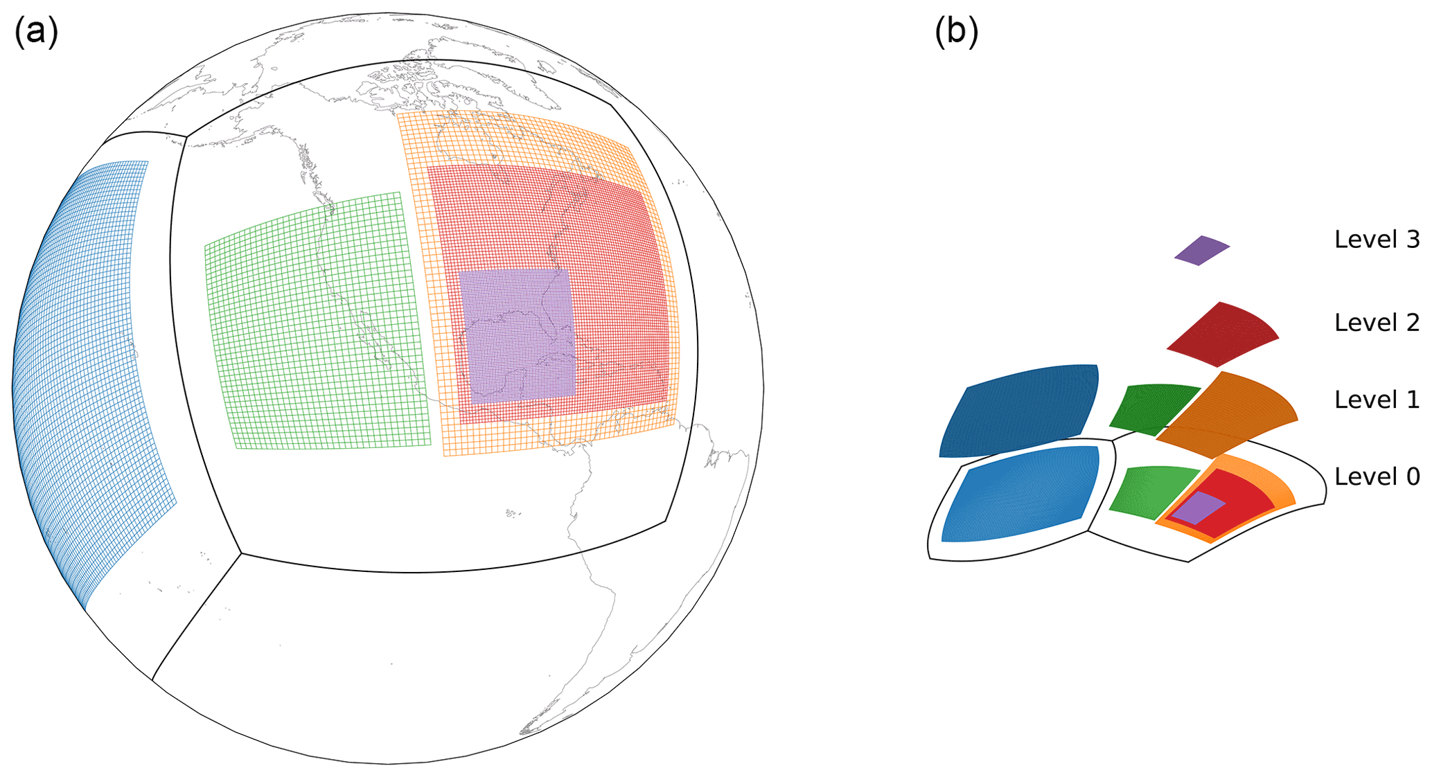
Figure 1 (a) schematic showing five nests in two tiles of the top-level parent grid in a global cubed-sphere configuration C48_5n2. (b) nest distribution across the levels: three nests on level 1, one nest on level 2 and one nest on level 3. Nests are then projected on level 0, showing their respective locations on two parent tiles of the cubed sphere.

3 Nesting methodology in FV3

3.1 Multiple nests

Building on the single-nest implementation developed by Harris and Lin (2013), the nesting capability in FV3 is extended to support multiple same-level and telescoping nested grids. These capabilities are fully functional within GFDL's FMS. A telescoping nest is defined as a nest within a nest. A global or regional grid is considered to be at level 0 and is called a top grid. A nest in one of the tiles (or tile) of the top grid (the grid at level 0) is considered to be a level 1 nest. A nest within the level 1 nest is considered as a level 2 nest (telescoping nest). There is no limit on the number of nests at a particular level (for instance, we can have multiple nests at level 1) and no limit on the number of levels as well. The nested grids are independent at the moment, meaning that there is no communication between nests at the same level. The communication occurs only between a child grid (nested grid) and its parent. A grid is considered as a parent grid if it holds a nest which is considered a child grid. For a telescoping case, in the example mentioned above, the nest at level 1 is a parent grid relative to the nest at level 2 but a child grid relative to the grid at level 0. So, a nest could be both a parent and a child grid at the same time. The nests at the same level can overlap (with no direct communication whatsoever) but are required to stay within their parent tile; this requirement may be relaxed in a forthcoming update. The communication between the nests and their parents is done per level. For instance, all nests present at a certain level (e.g., level 1) get their boundary condition data collectively from their parent level (level 0). For one-way updates, the updates occur sequentially by the level number, from top to bottom (level 0 to level 1, then level 1 to level 2, etc.). For two-way coupling, the updates occur in the opposite direction from last to second grid from last to top level. The time stepping on the nested grids is executed concurrently on different sets of processors, and the numerical parameters on each grid could be set differently and independently¹. Consequently, all these features make nesting a powerful and flexible tool tailored to be efficiently used on parallel supercomputers.

3.2 Child to parent grid communication

The nesting methodology is described in detail in Harris and Lin (2013) and will be summarized here. For each coarse cell, there are rf² (rf stands for refinement ratio) fine cells divided evenly in both horizontal directions. In the vertical direction, the parent and child could have a different number of vertical level. As discussed in the previous section, grid communication is only performed between a child grid and its parent. This could be roughly summarized in two steps:

1. All variables are spatially linearly interpolated from the parent grid to the nest ghost cells forming the nest boundary conditions. These boundary conditions are updated from the parent grid each remapping time step (dt_atmos/k_split). The nest's boundary conditions are also linearly extrapolated in time from two previous coarse grid solutions for every acoustic time step to allow the boundary conditions to evolve in time during the concurrent time stepping while waiting for the next boundary conditions from the parent grid at the next remapping time step. Linear interpolation processes are not conservative by nature which may introduce some artifacts in the boundary conditions. This is a matter of future investigation.

2. The two-way updates consists of averaging the fine grid data on the nest which will then replace the coarse grid data in the region where the child and parent grid overlap every large time step dt_atmos before updating the physics (this was found to maintain numerical stability). The fine-scalar variables are area-weight averaged over the overlap area and then replace the scalar in their parent coarse grid cell. The fine D-grid staggered variables are length-weight averaged only for the fine cells whose boundaries coincide with their parent coarse grid, thereby allowing vorticity conservation. Only the temperature and the three wind components are used for the two-way updates. Therefore, there is no violation of mass conservation during this process on the coarse grid. The smaller number of updated variables greatly reduces the data that needs to be passed between the grids, improving model efficiency especially for simulations with complex microphysical, aerosol or chemical schemes. In addition, since the air mass is different on both grids and since it determines the vertical coordinates, the nested averaged data is remapped to the coarse grid vertical coordinates, meaning that it is interpolated from its fine vertical coordinate to the parent coarse vertical coordinate. It is also worth mentioning that FV3 does allow partial two-way feedback, which is performed in the Rayleigh damping layer to reduce the effect of the update in the upper levels of the parent domain. This capability may be expanded in a future release of FV3.

Additional technical details can be found in Sect. 11.2 of Harris et al. (2021).

4 Global nesting – Hurricane Laura

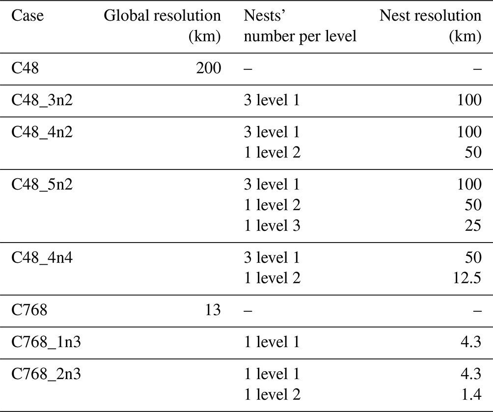
We consider simulations of Hurricane Laura's landfall in Louisiana (along the US coast with the northwestern Gulf of Mexico) in August 2020 using SHiELD for a range of resolutions with different nest layouts and refinement ratios as shown in Table 1. The initial conditions of all cases are considered at 12:00 Z on 26 August 2020, and all times shown thereafter are considered from this starting date. In the naming convention CA_BnC used thereafter, A refers to the number of grid cells per tile in each horizontal direction of the cubed sphere (there are $\text{A}\times \text{A}\times \mathrm{6}$ total cells on the parent cubed-sphere grid), B the number of nests and C the nests' corresponding refinement ratios. All nests of the same case have the same refinement ratio but the refinement ratio could be set differently for different cases. The size of the nest domains and the simulation computational cost are shown in Table A1.

Table 1 Simulation names and details. Global resolution corresponds to the resolution of the global grid or the top-level six tiles. The number of nests and their corresponding resolution are shown per level for each of the cases. Multiple nests per level have the same resolution.

4.1 Low-resolution global case C48

Simulations were performed using a global gnomonic grid C48 yielding an average global resolution of 2^∘ with an average grid cell of 200 km for the top grid. Nests of a constant refinement ratio were introduced in the following configuration, intended to demonstrate the ability of FV3 to contain multiple simultaneous nests: two nests located in tile 2 which was shifted and rotated to cover North America and one nest in tile 6 to cover part of the Pacific Ocean as can be seen in the Fig. 2a. The nests in tile 2 are laid out to, respectively, cover the western and eastern United States and surrounding waters. All of these nests are located at the first level, meaning that the communication occurs directly with their corresponding parent tiles. We will refer to this case as C48_3n2 where the corresponding nest resolution is approximately ∼100 km as shown in Table 1 and Fig. 2a.

Figure 2 (a) C48_3n2 grid layout showing the two nests over the east and west coasts in tile 6 and a third nest in the Pacific in tile 2; (b) C48_5n2 grid layout showing the two additional (to case C48_3n2) telescoping nests nested in the east coast nest. Grid size shown in both cases represents the actual real size of the grid.

For case C48_4n2, an additional nest is embedded in the nest of the east coast. The additional nest is, thereby, a level 2 telescoping nest whose parent grid is the aforementioned eastern US nest. The resulting telescoped nest resolution is ∼50 km. It is important to emphasize that the communication of the level two nest occurs with its parent nest of level 1 and not with the top grid at level 0 which is the six-tile cubed-sphere grid. Therefore, the one-way and two-way updates of the level 2 nest as described in the previous section occurs with the level 1 nest and at the same time the corresponding updates of the level 1 nest occur with the top level 0 grid.

For case C48_5n2, one more nest (a fifth nest) is added to the fourth nest of C48_4n2 as shown in Fig. 2b. The fifth nest yields an approximate resolution of ∼25 km as shown in Table 1. The corresponding three telescoping layouts are shown in Fig. 2b.

Figure 3 shows the global 850 mbar vorticity field on the top-level grid or level 0 for cases C48, C48_3n2, C48_4n2 and C48_5n2. Left and right columns correspond to 13 and 37 h after the initial time of 12:00 Z on 26 August. As can be seen, Hurricane Laura is completely dissipated for case C48, which is expected since the resulting grid is too coarse (200 km) to capture any details of the event.

Figure 3 Global domain 850 mbar vorticity time evolution showing Hurricane Laura's landfall. Left column corresponds to 13 h; right column corresponds to 37 h for cases C48, C48_3n2, C48_4n2 and C48_5n2 from top to bottom. Black lines represent nest boundaries.

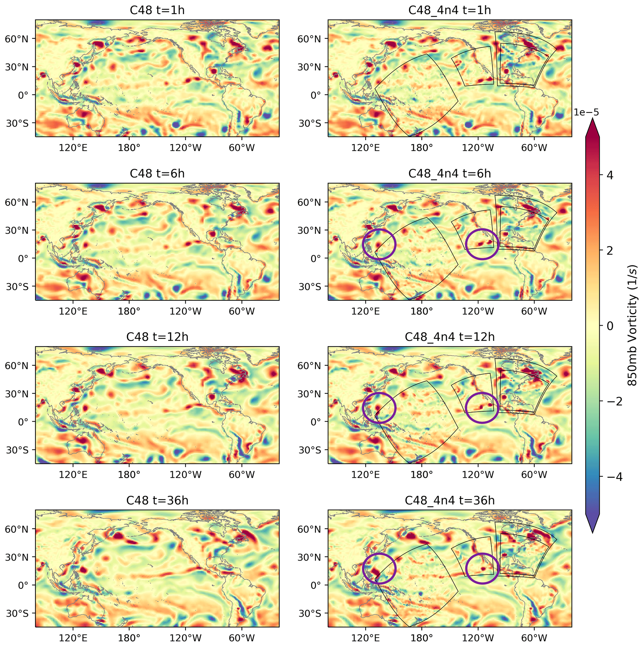
Figure 4 Global domain 850 mbar vorticity time evolution showing Hurricane Laura's landfall. Left column corresponds to case C48; right column corresponds to case C48_4n4. Top to bottom rows correspond to times of 1, 6, 12 and 36 h. Darker colors represent higher vorticity. The circles point to the weather activity in west Mexico and Typhoon Maysak. Black lines represent nest boundaries.

Considering the nested cases C48_3n2, C48_4n2 and C48_5n2, the feedback from the nest in the Pacific and the nest on the west coast to the top grid lead to finer structures present at those locations compared to the raw case of C48. Coming back to Hurricane Laura, C48_3n2 is able to capture its landfall with a nest resolution of 100 km; however, this resolution is still too coarse as we can see from the diffusive structure of the hurricane which starts to spread on a wider area and does not present a compact structure like the one seen in cases C48_4n2 and C48_5n2.

Figure 4 shows the global 850 mbar vorticity field on the top-level grid for cases C48 and C48_4n4. Rows from top to bottom correspond to 1, 6, 12 and 36 h after the initial time of 12:00 Z on 26 August. C48_4n4 is similar to the previous nested case C48_4n2 but with finer nests: the refinement ratio is equal to 4 for all four nests which yields a resolution of 50 km on for the three level 1 nests and a resolution of 12.5 km for the telescoping nest level 2 on Laura's landfall. From the 850 mbar vorticity field, we can clearly see finer structures in the region where the nest and parent grid overlap due to the two-way coupling. C48_4n4 is able to capture the landfall of Hurricane Laura, the evolution of the intense weather activity in the Gulf of Tehuantepec and the initial stages of formation of Typhoon Maysak in the Pacific. The circles point to the weather activity in Mexico and Typhoon Maysak. It is worthwhile to note that C48 was able to capture Typhoon Maysak but the initial stages of its formation are not captured in detail as in the case of the higher-resolution nest of C48_4n4 over that region. The feedback from nests of high refinement ratios is more pronounced compared to lower refinement ratio nests as can be seen on the west coast and the Pacific regions of case C48_4n4 compared to cases C48_3n2, C48_4n2 and C48_5n2.

Hurricane Laura's landfall on the first level nest (resolution 100 km) is shown in Fig. 5 for cases C48_3n2, C48_4n2 and C48_5n2 at times of 12, 24 and 36 h. As previously discussed, the hurricane structure in case C48_3n2 is more diffusive than the other cases as seen in the plots of the first row. On the other hand, due to the two-way feedback of the higher-resolution nests of cases C48_4n2 and C48_5n2, the corresponding hurricane structure presents a more compact form, and finer details are seen in the regions where the nested and parent grids overlap.

The hurricane structure on the first level nest is very comparable for cases C48_4n2 and C48_5n2, as can be seen in the plots of the last two rows; however, some differences still exist in that area due to the additional nest of case C48_5n2. Indeed, looking at Fig. 6, which shows the hurricane evolution on the second level nest of resolution 50 km, the hurricane structure is very comparable in both cases with more detailed finer structures in case C48_5n2 due to the two-way feedback coming from the third level nest resolution of 25 km.

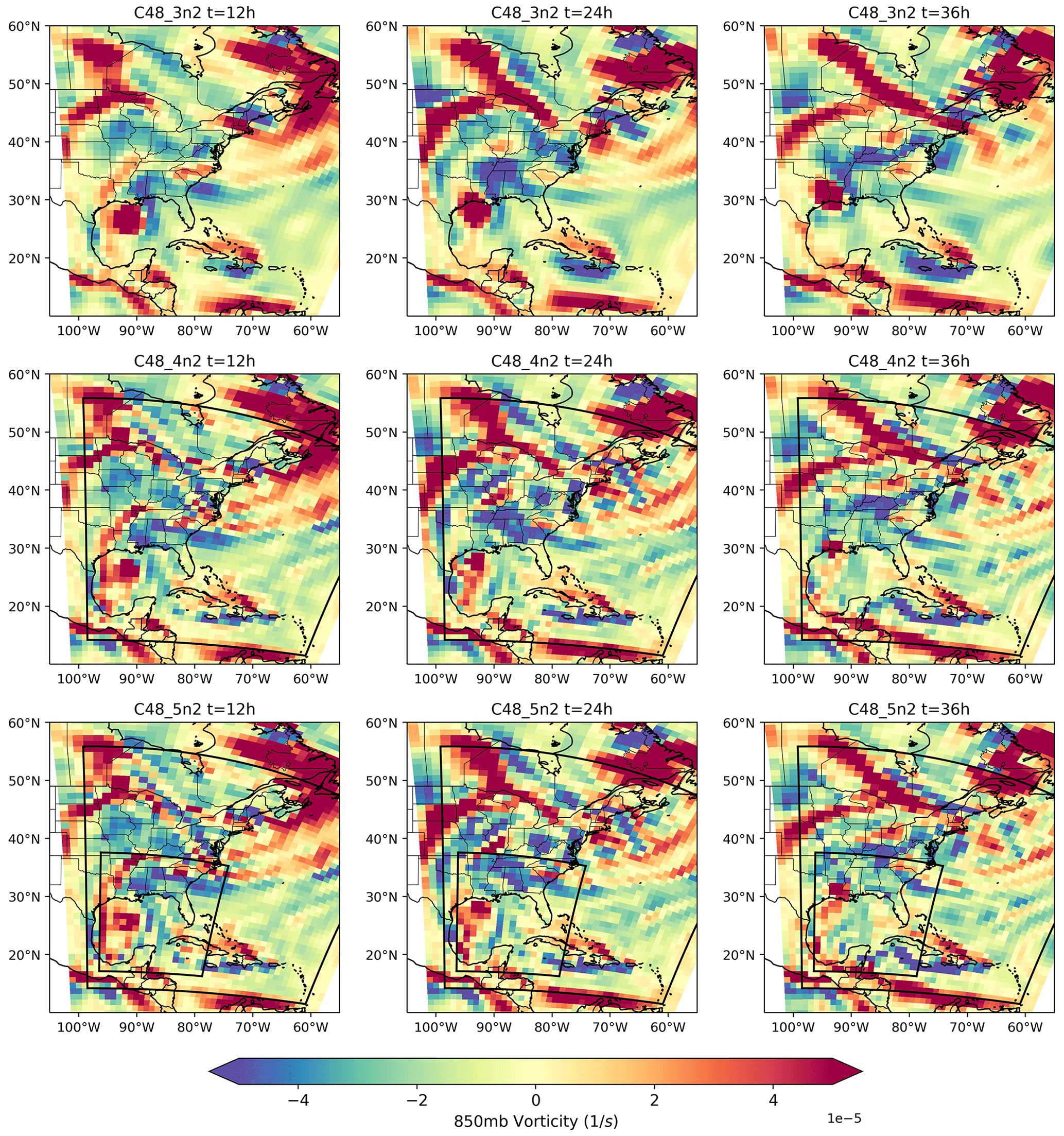
Figure 5 First level nest 850 mbar vorticity time evolution showing Hurricane Laura's landfall. Top to bottom rows correspond to cases C48_3n2, C48_4n2, C48_5n2, respectively. Left to right correspond to 12, 24 and 36 h. Black lines represent nest boundaries.

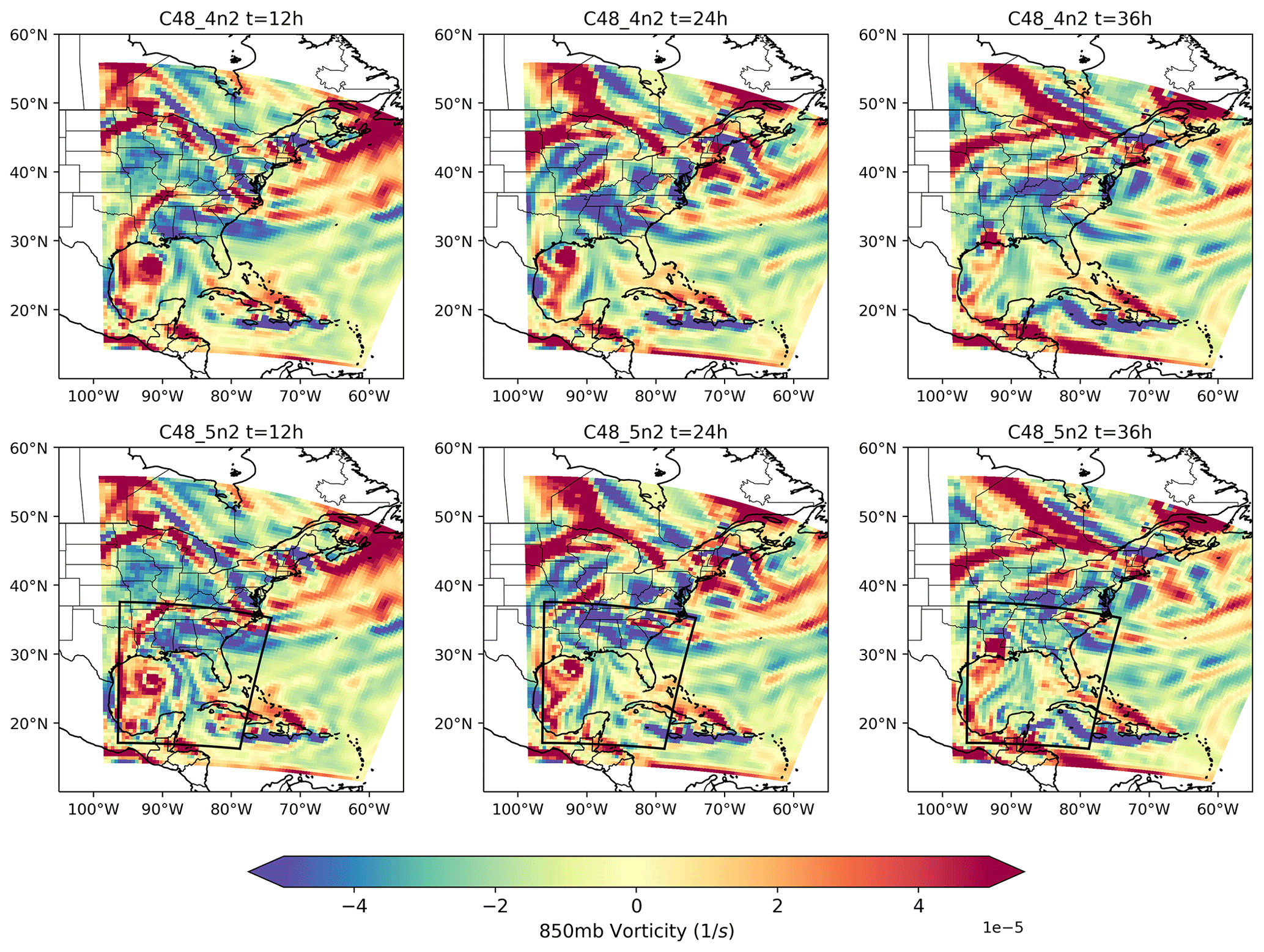
Figure 6 Second level nest 850 mbar vorticity time evolution showing Hurricane Laura's landfall. Top to bottom rows correspond to cases C48_4n2, C48_5n2, respectively. Left to right correspond to 12, 24 and 36 h. Black lines represent nest boundaries.

Figure 7 Finest grid surface wind speed time evolution showing Hurricane Laura's landfall at times of t=9, 18 and 27 h in cases C48 (200 km), C48_3n2 (100 km), C48_4n2 (50 km), C48_5n2 (25 km) and C48_4n4 (12.5 km). White lines correspond to velocity contours starting at 30 m s⁻¹ with increments of 5 m s⁻¹.

Figure 7 shows snapshots of the 2-D surface wind on the finest grid of all low-resolution global cases – C48 (200 km), C48_3n2 (100 km), C48_4n2 (50 km), C48_5n2 (25 km) and C48_4n4 (12.5 km) – at durations of 9, 18 and 27 h. In accordance with the vorticity plots discussed earlier, decreasing the resolution results in a diffusive storm structure while increasing the resolution by using multiple level nests and varying the refinement ratio yields a more detailed description of the storm evolution. Coarse resolutions down to 100 km are incapable of capturing any of the hurricane structures, while finer resolutions of 50 km down to 12.5 km such as in the cases of C48_4n2 (50 km), C48_5n2 (25 km) and C48_4n4 (12.5 km) were capable of gradually capturing the location of the hurricane structures such as the eye and high-wind region. In addition, since more details are captured with increasing resolution, the hurricane intensity increases with nesting levels as can be seen by the contour plots (starting at 30 m s⁻¹) of the surface wind speed. The wind contours offsets become smaller closer to the eye with increased resolution, indicating the presence of stronger winds in that region.

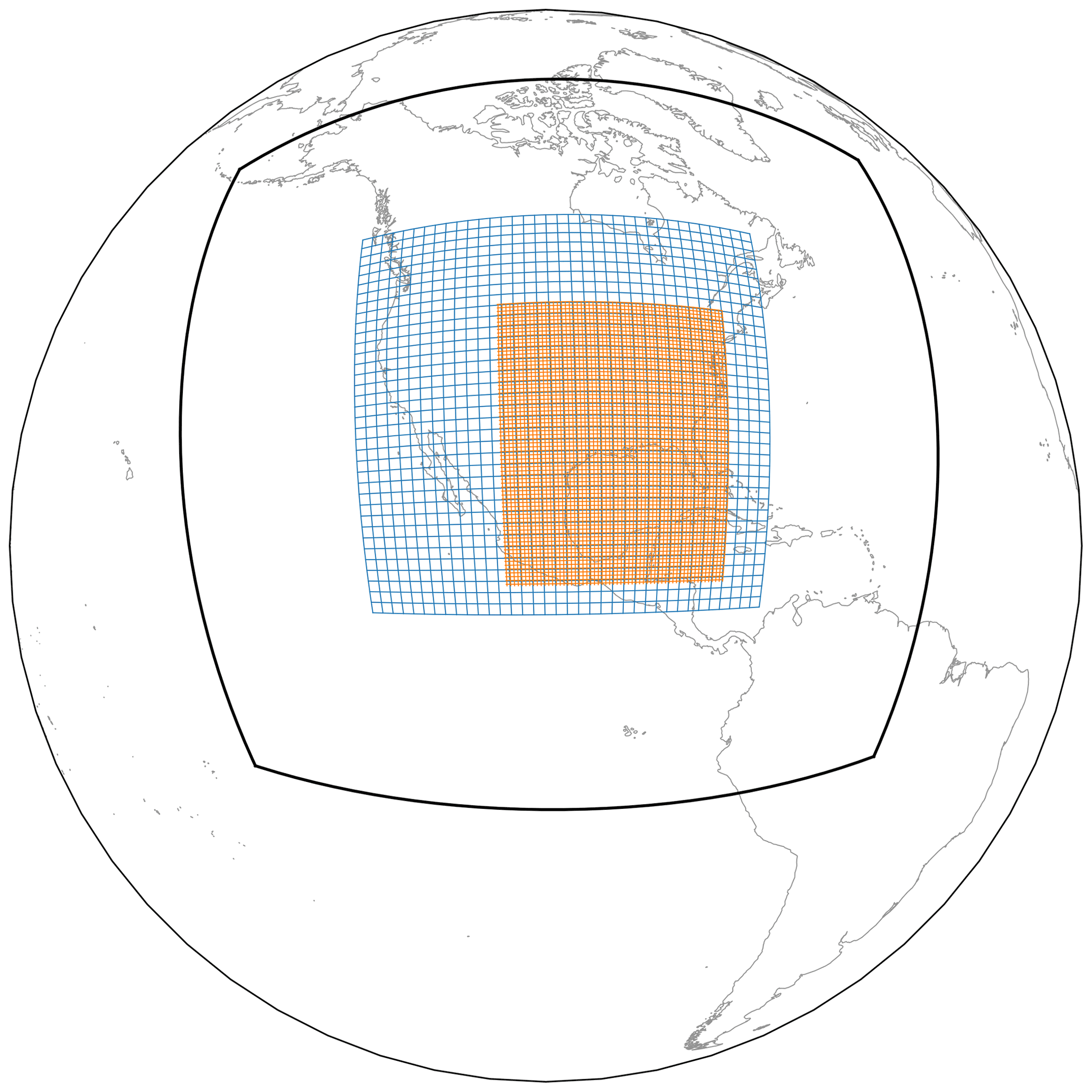
Figure 8 C768_2n3 grid layout showing the location of the level 1 and level 2 telescoping nests. The boundaries of the top parent tile are shown. The number of cells of the nested grids is reduced by a factor of 900.

4.2 High-resolution global case C768

Simulations of the same event, Hurricane Laura, were performed with a higher-resolution C768 global domain with an average grid width of 13 km. In addition, cases with one nest, C768_1n3, and two nests, C768_2n3, centered on the east coast over the hurricane were considered. The C768_2n3 is simply a C768_1n3 with a telescoping nest: a level 2 nest is embedded in the level 1 nest as shown in Fig. 8. The resulting grid resolution of the nests is, consequently, 4.3 km for the first level nest and 1.4 km for the telescoping nest as shown in Table 1.

Figure 9 shows the time evolution of 2-D surface wind speed on the finest grid of cases C768, C768_1n3 and C768_2n3 at 9, 18 and 27 h with a corresponding approximate resolution of 13, 4.3 and 1.4 km from top to bottom. Finer details are captured when going to higher resolution, similar to the results of the previous section. The added detail is especially notable near Laura's center. It is also worth noting that the storm travels slower in the high-resolution case as seen by the location of the eye: the eye reaches the coast faster in case C768_1n3 compared to C768_2n3, which is a matter of future investigation.

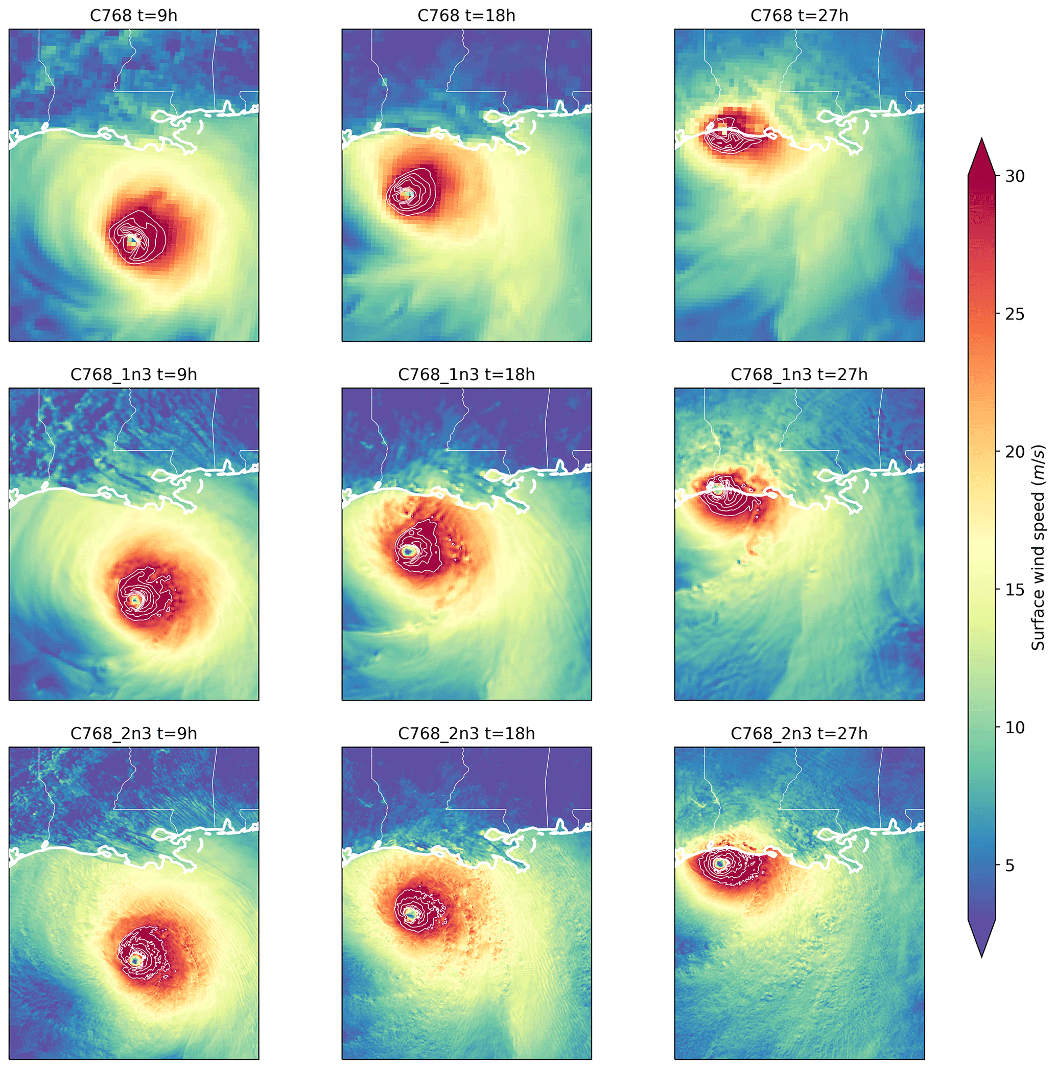
Figure 9 Finest grid surface wind speed time evolution showing Hurricane Laura's landfall at times of t=9, 18 and 27 h in cases C768 (13 km), C768_1n3 (4.3 km) and C768_2n3 (1.4 km). White lines correspond to velocity contours starting at 30 m s⁻¹ with increments of 5 m s⁻¹.

Figure 10 Column-integrated water vapor (PWATclm), hourly accumulated precipitation (PRATsfc) and hourly accumulated precipitation due to convection parameterization (CPRATsfc), all shown at time of 18 h on the finest grid of cases C768, C768_1n3 and C768_2n3. The color scale was selected to capture light and heavy rain.

Figure 10 shows the column-integrated water vapor, the hourly accumulated precipitation and the hourly accumulated precipitation due to convection parameterization at t=18 h on the finest grid of C768, C768_1n3 and C768_2n3. Similar to the velocity field results, finer details are captured with increasing resolutions. The intensity of rain seems to increase with increased resolution and becomes more localized when looking at the 1 km nest. The position of these small-scale features of high intensity indicates the geographic location where most of the storm damage is likely to occur. On the other hand, the precipitation due to convection parameterization decreases in intensity with increasing resolution. This is expected since higher resolution will resolve the bulk of the precipitation and thus the contribution coming from parameterization will be minimal and the contribution of the resolved precipitation will be maximal as previously mentioned. Note that the heaviest rain rates even at 13 km resolution are from the resolved-scale precipitation. The right column of Fig. 10 also clearly shows the scale awareness of the SAS convection scheme (Han et al., 2017) as it becomes less active at higher resolutions, a valuable asset for our multi-scale modeling.

4.3 Quantitative analysis

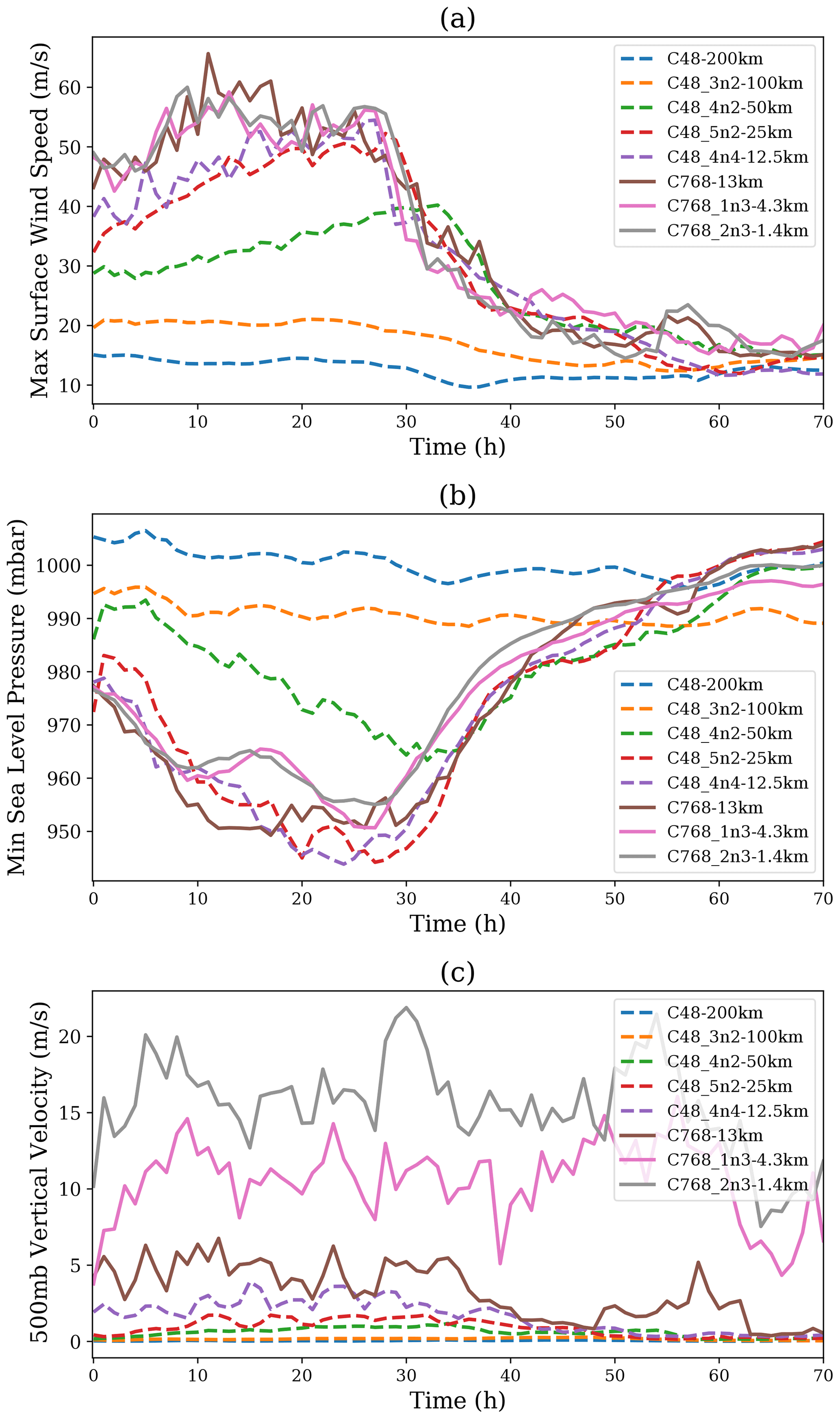
Figure 11 shows the time evolution of (a) maximum surface wind speed, (b) the minimum sea level pressure and (c) 500 mbar vertical updraft of the finest nested grid of each of the low- and high-resolution cases shown in Table 1. For instance, for case C768_2n3, we show the evolution on the level 2 nest of a 1.4 km resolution; for case C48_4n4, the results of the 12.5 km nest are shown and so on. The lower-resolution cases C48 and C48_3n2 present constant values for the three variables as time advances. This shows that a coarse resolution down to 100 km is incapable of capturing the event. For all other cases, we notice an overall increase in storm intensity with nesting levels or with increasing resolution. The maximum surface wind speed increases in magnitude from the initial time to reach a peak of approximately 60 m s⁻¹ between 10 and 20 h for cases C768, C768_1n3 and C768_2n3. Then, it starts to decrease between 25 and 30 h, setting the mark of the beginning of the landfall. Those three curves almost overlap, showing that a minimum resolution of 13 km might be enough to capture the maximum surface wind speed time evolution. For the intermediate resolutions, we notice an increase of surface wind speed magnitude with an increase of nesting level with a delayed peak to around 25 h; however, this starts to decrease shortly after this time for all cases.

A similar behavior is seen for the minimum sea level pressure. A minimal coarse resolution of 100 km is unable to capture the event. All cases reach a minimum of 950 mbar some time between 10 and 30 h, then decrease at the 30 h mark. The sea level pressure decreases with increasing resolution; however, we notice that the high-resolution cases C768_1n3 and C768_2n3 present a slightly higher minimum sea pressure compared to cases C768, C48_5n2 and C48_4n2, which is a matter of future investigation.

The 500 mbar vertical velocity increases systematically with increasing resolution to reach a value 20 m s⁻¹ for the highest-resolution nest. As seen in the plot, the curves corresponding to resolutions coarser than 13 km almost overlap, and the curves' offset starts to increase from a 13 km resolution to the 1 km nest. This shows that while a 13 km resolution looks enough to capture an approximate trend of the time evolution of the velocity and pressure fields, a higher resolution is still required to capture to the 500 mbar vertical updraft.

Finally, the results of cases C48_4n4 (12.5km) and C768 (13 km) are broadly similar, showing that telescoping nesting in a low-resolution global setup is able to capture the evolution of the event similar to a high-resolution global case. In addition, the C48_4n4 telescoping setup is still computationally less expensive than the C768 uniform domain, as discussed in Sect. 6.

Figure 11 Time evolution of (a) maximum surface wind speed, (b) the minimum sea level pressure and (c) 500 mbar vertical updraft of the finest nested grid in each of the cases shown in Table 1.

5 Regional nesting – atmospheric river

We now show nested grid simulations of an atmospheric river striking the US west coast in late January 2021 (https://cw3e.ucsd.edu/cw3e-event-summary-26-29-january-2021/, last access: 30 May 2022) within a parent regional domain, to demonstrate the capabilities of nesting with a regional instead of a global domain. The regional domain is described fully by Black et al. (2021). Several subsequent publications (Dong et al., 2020; Clark et al., 2022) have shown that FV3-based regional models have been proven to be quite useful, yielding good short-range forecasts (0–48 h) while using less computational resources than a global-nest domain. The setup consists of a regional domain spanning from the eastern Pacific to the west coast, embedding two subsequent level 1 and level 2 nests, as shown in Fig. 12. Grid 1 is the outermost regional domain, while grids two and three correspond to the level 1 and level 2 nests. All nests are factor-of-3 refinements, giving a configuration of an approximate resolution of 50–17–6 km, as shown in Table 2. The simulations are initialized at 00:00 Z on 26 January 2021. The size of the nest domains and the simulation computational cost are shown in Table A1.

Figure 12 shows the precipitation rate at t=48 h on the highest-resolution tile of all three cases and superposing the grids in the following order: (a) tile one of R192, (b) tile one of R192 and tile two of R192_1n3 and (c) tile one of R192, tile two of R192_1n3 and tile three of R192_2n3. Results show that increasing the resolution from top to bottom allows capturing finer details in the region where the nested grids are located. Moreover, it is apparent that the gross features of the weather system are the same for all of the simulations, indicating that the nests are not distorting the structure of the atmospheric river. Most notably, despite the abrupt refinement and the significant increase in detail on the successively finer grids, the rain band structures are continuous across the grid interfaces and are free of any apparent numerical artifacts.

Figure 13 shows the accumulated frozen precipitation during the three simulated days. The frozen precipitation is defined as the depth of liquid-water equivalent to the frozen precipitation that has fallen. From left to right, the results are shown, respectively, for the highest-resolution grids of R192, R192_1n3 and R192_2n3. Higher-resolution nests give a more detailed description of geographic distribution of the orographic frozen precipitation. In addition, enhanced resolution is able to capture more intense snowfall in some areas, which is in accordance with the results of the previous section.

This case illustrates the usage of multiple and telescoping nesting in a regional domain and shows that the nest boundaries at different levels do not introduce severe discontinues in coarser solutions. In addition, higher-resolution grids tend to capture finer and more intense details of any weather event whether the top parent grid is a global or regional domain.

Table 2 Simulation names and details. Regional resolution corresponds to the resolution of the regional grid or the top-level one-tile grid. The number of nests and their corresponding resolution are shown per level for each of the cases.

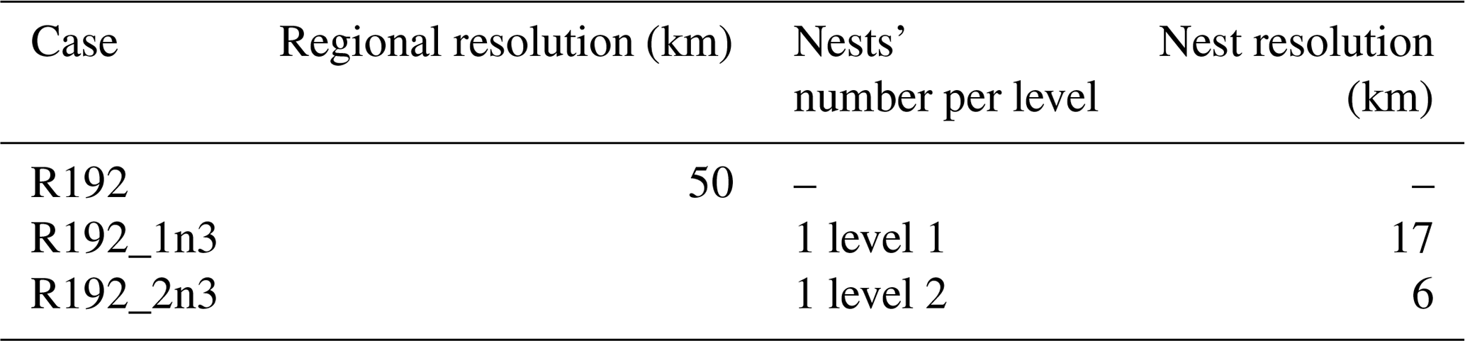
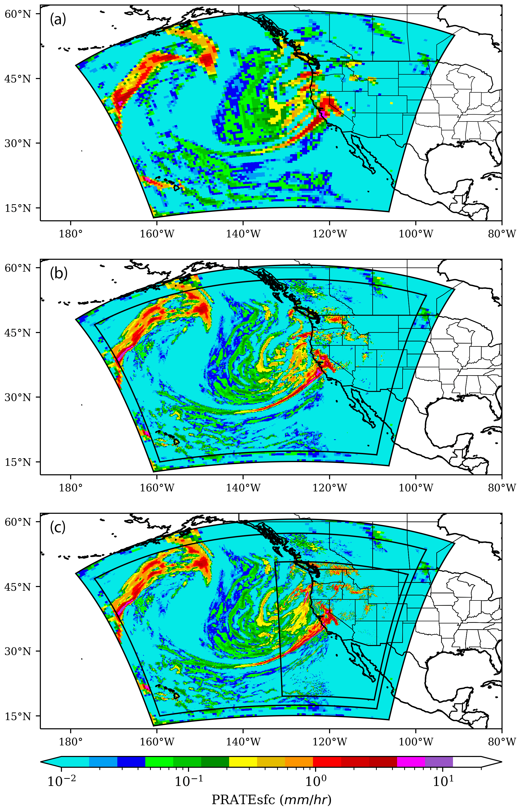
Figure 12 Hourly accumulated precipitation (PRATsfc) at t=48 h (a) R192, (b) R192_1n3 and (c) R192_2n3.

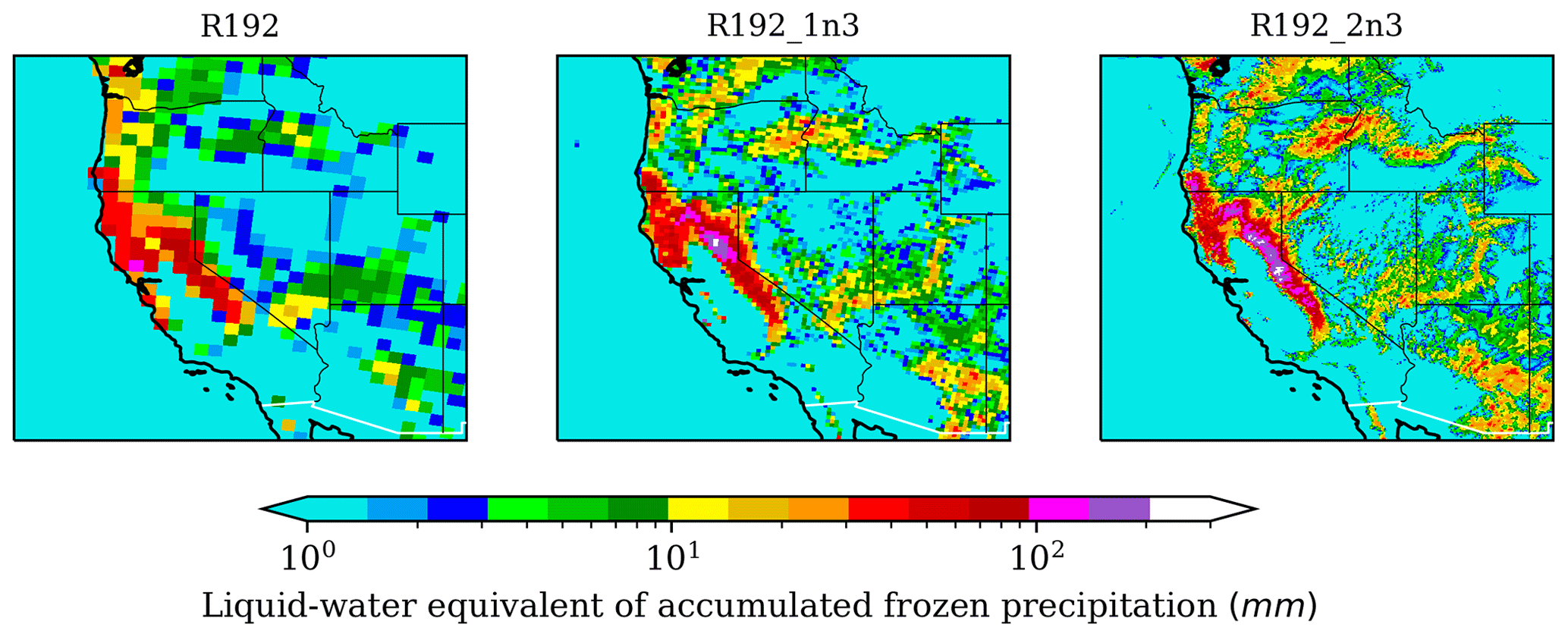
Figure 13 Total 3 d accumulated frozen precipitation, given as liquid-water equivalent, for R192, R192_1n3 and R192_2n3.

6 Code timing and performance

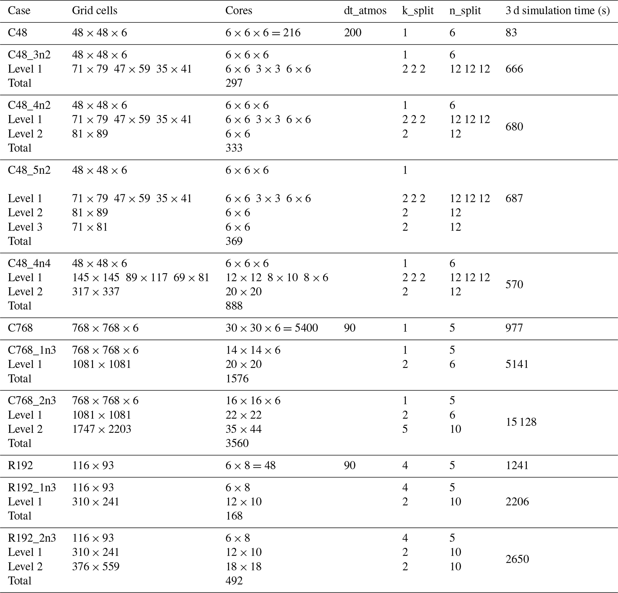
The size of all nest domains, time step details, number of cores and simulation time for all cases are shown in Table A1. n_split was chosen to be in the interval [5,12], and k_split was chosen in a way to get an appropriate Courant number for the different grids. It is clearly obvious that a low-resolution global grid with high-resolution multiple nests requires less computational resources than a high-resolution global grid. In fact, if one is interested in one or more particular events, such as the landfall of Hurricane Laura, using a C48_4n4 setup is much cheaper than a global C768. The telescopic nest of C48_4n4 spanning over the east coast yields a resolution of 12.5 km which is similar to the 13 km of C768. The C48_4n4 requires 140 core hours to simulate a 3 d simulation, whereas a C768 case requires 1465 core hours. This is a 10× reduction in computational resources. In addition, concurrent nesting allows the user to consider additional nests on more cores without compromising the run time of a case. This can be seen by looking at the respective timings 680 and 687 s of C48_4n2 and C48_5n2, where adding a level 3 nest with 36 cores for case C48_5n2 did not degrade the run time of the 3 d simulation. It is worth mentioning that not all cases in Table A1 are fully optimized to get the best computational performance, and further performance improvements may be possible.

7 Conclusions

We present, in this study, the multiple same-level and telescoping two-way nesting capability implemented in the Geophysical Fluid Dynamics Laboratory Finite-Volume Cubed-Sphere Dynamical Core (FV3). Simulations were performed within GFDL's weather model SHiELD with low and high resolutions and multiple same-level and multi-level telescoping nests under both global and regional configurations. Hurricane Laura's landfall was simulated with both low- and high-global-resolution setups with multiple nests with resolutions spanning from 200 km down to 1 km. In addition, for the low-resolution global setup, nests were spread out over the globe covering different geographic locations of interest and were able to capture several independent and simultaneous weather events such as the initial stages of formation of Typhoon Maysak and intense weather activity at the western gulf of Mexico. The multi-level telescoping nesting capability was shown to work well in capturing fine-scale flow features during the landfall of Hurricane Laura at different nest levels. The intensity of the storm increased up to a certain resolution. The velocity magnitude and sea level pressure showed a similar behavior during the landfall. Precipitation and moisture increased with increased resolution as well. Two-way nesting updates, at various telescoping levels, were shown not to introduce numerical artifacts to their corresponding parent grids at the cells where the nest boundaries overlap with their corresponding coarse cells.

Additionally, an atmospheric river event that hit California in January 2021 was simulated in SHiELD in a regional setup. Two nests forming a telescoping setup were considered. The rainfall and total 3 d accumulated frozen precipitation were found to increase with increased resolution. In addition, higher resolutions gave a more detailed description of the geographic distribution of these precipitations. Furthermore, the precipitation rain bands presented a continuous pattern when crossing a nest boundary when overlaying the fine solution on the coarse one, emphasizing the lack of artifacts of the current two-way nesting algorithm.

Furthermore, concurrent multiple nesting has been shown to require less computational resources than a global setup of a comparable resolution. In addition, additional nests do not compromise the performance of a simulation setup if the number of cores is distributed among the grids in a optimal manner.

Multiple nesting within FV3 was made publicly available as of the 202107 release (https://github.com/NOAA-GFDL/GFDL_atmos_cubed_sphere/releases/tag/FV3-202107-public, last access: 30 May 2022). Current and future efforts will focus on developing algorithms to enable moving nests to track weather events such as tropical storms. In addition, nests spanning multiple tiles are currently supported by the FMS infrastructure and will be implemented in the dynamical core FV3.

Appendix A

Table A1 Number of grid cells, cores, remapping time steps per dt_atmos, acoustic time steps per k_split and simulation time of all runs. Number of grid cells and cores are shown on the same line for all nests at the same level. These runs could still be optimized by redistributing the number of cores among grids in a more efficient way, but this is not pursued here.