Global, high-resolution mapping of tropospheric ozone – explainable machine learning and impact of uncertainties

Tropospheric ozone is a toxic greenhouse gas with a highly variable spatial distribution which is challenging to map on a global scale. Here, we present a data-driven ozone-mapping workflow generating a transparent and reliable product. We map the global distribution of tropospheric ozone from sparse, irregularly placed measurement stations to a high-resolution regular grid using machine learning methods. The produced map contains the average tropospheric ozone concentration of the years 2010–2014 with a resolution of 0.1^∘ × 0.1^∘. The machine learning model is trained on AQ-Bench (“air quality benchmark dataset”), a pre-compiled benchmark dataset consisting of multi-year ground-based ozone measurements combined with an abundance of high-resolution geospatial data.

Going beyond standard mapping methods, this work focuses on two key aspects to increase the integrity of the produced map. Using explainable machine learning methods, we ensure that the trained machine learning model is consistent with commonly accepted knowledge about tropospheric ozone. To assess the impact of data and model uncertainties on our ozone map, we show that the machine learning model is robust against typical fluctuations in ozone values and geospatial data. By inspecting the input features, we ensure that the model is only applied in regions where it is reliable.

We provide a rationale for the tools we use to conduct a thorough global analysis. The methods presented here can thus be easily transferred to other mapping applications to ensure the transparency and reliability of the maps produced.

1 Introduction

Tropospheric ozone is a toxic trace gas and a short-lived climate forcer (Gaudel et al., 2018). Contrary to stratospheric ozone which protects humans and plants from ultraviolet radiation, tropospheric ozone causes substantial health impairments to humans because it destroys lung tissue (Fleming et al., 2018). It is also the cause of major crop loss, as it damages plant cells and leads to reduced growth and seed production (Mills et al., 2018). Tropospheric ozone is a secondary pollutant with no direct sources but with formation cycles depending on photochemistry and precursor emissions. It is typically formed downwind of precursor sources from traffic, industry, vegetation, and agriculture, under the influence of solar radiation. Ozone patterns are also influenced by the local topography causing specific flow patterns (Monks et al., 2015; Brasseur et al., 1999). Depending on the on-site conditions, ozone can be destroyed in a matter of minutes or have a lifetime of several weeks with advection from source regions to remote areas (Wallace and Hobbs, 2006). The interrelation of these factors of ozone formation, destruction, and transport is not fully understood (Schultz et al., 2017). This makes ozone both difficult to quantify and to control. Public authorities recognize ozone-related problems. They install air quality monitoring networks to quantify ozone (Schultz et al., 2015, 2017). Furthermore, they enforce maximum exposure rules to mitigate ozone health and vegetation impacts (e.g., European Union, 2008).

Currently, there is increased use of machine learning methods in tropospheric ozone research. Such “intelligent” algorithms can learn nonlinear relationships of ozone processes and connect them to environmental conditions, even if their interrelations are not well understood through process-oriented research. Kleinert et al. (2021) and Sayeed et al. (2021) used convolutional neural networks to forecast ozone at several hundred measurement stations, based on meteorological and air quality data. Large training datasets allowed them to train deep neural networks, resulting in a significant improvement over the first machine learning attempts to forecast ozone (Comrie, 1997; Cobourn et al., 2000). Machine learning is also used to calibrate low-cost ozone monitors that complement existing ozone monitoring networks (Schmitz et al., 2021; Wang et al., 2021). Furthermore, compute-intensive chemical reactions schemes for numerical ozone modeling can be emulated using machine learning (Keller et al., 2017; Keller and Evans, 2019). Ozone datasets which are used as training data for machine learning models are increasingly made available as FAIR (Wilkinson et al., 2016) and open data. AQ-Bench (“air quality benchmark dataset”, Betancourt et al., 2021b), for example, is a dataset for machine learning on global ozone metrics and serves as training data for this mapping study.

We refer to mapping as a data-driven method for spatial predictions of environmental target variables. For mapping, a model is fit to observations of the target variable at measurement sites, which might even be sparse and irregularly placed. Environmental features are used as proxies for the target variable to fit the model. A map of the target variable is produced by applying the model to the spatially continuous features in the mapping domain. Mapping for environmental applications has been performed since the 1990s (Mattson and Godfrey, 1994; Briggs et al., 1997). It was deployed for air pollution as an improvement over spatial interpolation and dispersion modeling, which suffer from performance issues due to sparse measurements, and lack of detailed source description (Briggs et al., 1997). Hoek et al. (2008) describe these early mapping studies as “linear models with little attention to mapping outside the study area”. In contrast, modern machine learning algorithms are often trained on thousands of samples for mapping (Petermann et al., 2021; Heuvelink et al., 2020). Several studies (e.g., Li et al., 2019; Ren et al., 2020) have shown that mapping using machine learning methods is superior to other geostatistical methods such as Kriging because it can capture nonlinear relationships and makes ideal use of environmental features by exploiting similarities between distant sites. In contrast to traditional interpolation techniques, mapping allows to extend the domain to the global scale, because it can predict the variable of interest based on environmental features, even in regions without measurements (Lary et al., 2014; Bastin et al., 2019; Hoogen et al., 2019). Recently, it is questioned whether machine learning methods are the most suitable to “map the world” (Meyer, 2020): Meyer et al. (2018) and Ploton et al. (2020) point out that some studies may be overconfident because they validate their maps on data that are not statistically independent from the training data. This occurs when a random data split is used on data with spatiotemporal (auto)correlations. There are also concerns when the mapping models are applied to areas that have completely different properties from the measurement locations (Meyer and Pebesma, 2021). A model trained on certain input feature combinations can only be applied to similar feature combinations. Furthermore, uncertainty estimates of the produced maps are important as they are often used as a basis for further research.

In this study, we produce the first fully data-driven global map of tropospheric ozone, aggregated in time over the years 2010–2014. This study builds upon Betancourt et al. (2021b) who proved that ozone metrics can be predicted using static geospatial data. We provide the map as a product and combine it with uncertainty estimates and explanations to ensure the trustworthiness of our results. We justify the choice of methods and clarify why they are necessary for a thorough global analysis. Section 2 contains a description of the data and machine learning methods, including explainable machine learning and uncertainty estimation. Section 3 contains the results, which are discussed in Sect. 4. We conclude in Sect. 5.

2 Data and methods

2.1 Data description

In this section, we present the datasets used in this study. Technical details on these data are given in Appendix A.

Figure 1 Average ozone statistic of the AQ-Bench dataset. The values at 5577 measurement stations are aggregated over the years 2010–2014. (a) Values on a map projection. (b) Histogram and summary statistics.

2.1.1 AQ-Bench dataset

We fit our machine learning model on the AQ-Bench dataset (“air quality benchmark dataset”, Betancourt et al., 2021b). The AQ-Bench dataset is a machine learning benchmark dataset that allows to relate ozone statistics at air quality measurement stations to easy-access geospatial data. It contains aggregated ozone statistics of the years 2010–2014 at 5577 stations around the globe, compiled from the database of the Tropospheric Ozone Assessment report (TOAR, Schultz et al., 2017). The AQ-Bench dataset considers ozone concentrations on a climatological time scale instead of day-to-day air quality data. The scope of this dataset is to discover purely spatial relations. Machine learning models trained on this dataset will output aggregated statistics over the years 2010–2014 and will not be able to capture temporal variances. This is beneficial if the required final data products are also aggregated statistics. The majority of the stations are located in North America, Europe, and East Asia. The dataset contains different kinds of ozone statistics such as percentiles or health-related metrics. This study focuses on the average ozone statistic as the target (Fig. 1).

The features in the AQ-Bench dataset characterize the measurement site and are proxies for ozone formation, destruction, and transport processes. For example, the “altitude” and “relative altitude” of the station are important proxies for local flow patterns and ozone sinks. “Population density” in different radii around every station are proxies for human activity and thus ozone precursor emissions. “Latitude” is a proxy for ozone formation through photochemistry, as radiation and heat generally increase towards the Equator. The land cover variables are proxies for precursor emissions and deposition. The full list of features and their relation to ozone processes are documented by Betancourt et al. (2021b). Figure 2 shows predictions of a machine learning model on the test set of AQ-Bench. Table 1 lists all features used in this study.

Figure 2 Predicted ozone values versus measurement values of the test set of the AQ-Bench dataset. See Sect. 3.3.1 for the specifications of the used machine learning model.

2.1.2 Gridded data

Features are needed on a regular grid (i.e., as raster data) over the entire mapping domain to map the target average ozone. The original gridded data used here (Appendix Sects. A and B) has a resolution of 0.1^∘ × 0.1^∘ or finer. Since our target resolution is 0.1^∘ × 0.1^∘, the gridded data are downscaled to that resolution if the original resolution is finer. The “land cover”, “population”, and “light pollution” features of the AQ-Bench dataset are spatial aggregates in a certain radius around the station (see Table 1). To prepare gridded fields of these features, the area around each individual grid point is considered, and the required radius aggregation is written to that grid point. The gridded dataset is available under the DOI https://doi.org/10.23728/b2share.9e88bc269c4f4dbc95b3c3b7f3e8512c (Betancourt et al., 2021c).

Table 1 Features selected from the AQ-Bench dataset.

2.2 Explainable machine learning workflow

We apply a standard mapping workflow and extend it with explainable machine learning methods as described in this section. Together with the uncertainty assessment methods described in Sect. 2.3, they allow for a thorough analysis of our machine learning model. A random forest (Breiman, 2001) is fit on the AQ-Bench dataset to predict average ozone for given features. A random forest is an ensemble of regression trees that is created by bootstrapping the training dataset to increase generalizability. We choose random forest because tree-based models are the state of the art for structured data (Lundberg et al., 2020). Random forest was also shown to outperform linear regression and a shallow neural network in predicting average ozone on the AQ-Bench dataset (Betancourt et al., 2021b). In addition, this algorithm has been proven to be suitable for mapping in several studies (Petermann et al., 2021; Nussbaum et al., 2018; Ren et al., 2020). We use the Python framework SciKit-learn (Pedregosa et al., 2011) for machine learning and hyperactive (Blanke, 2021) for hyperparameter tuning.

A proper validation strategy is crucial for spatial prediction models because both environmental conditions and target variables are often correlated in space. When tested on spatially correlated and thus statistically dependent samples, mapping results may be overconfident (Meyer et al., 2018; Ploton et al., 2020). We use the independent spatial data split provided with the AQ-Bench dataset to validate spatial generalizability. Details on our validation strategy are given in Sect. 2.2.1.

As an extension of the standard mapping workflow described in Sect. 1, we perform experiments to increase interpretability, test robustness, and explain the model. The extended workflow is summarized in Table 2 and further justified in the following.

Table 2 Machine learning experiments as an addition to the standard mapping method. For details on the methods, refer to the given sections.

The use of redundant features in mapping applications can favor spatial overfitting. We thus remove counterproductive features by forward feature selection as proposed by Meyer et al. (2018). Additionally, we apply basic feature engineering to increase the interpretability of the model. Details on feature engineering and feature selection are described in Sect. 2.2.2. In order to make our mapping model trustworthy, we verify its robustness and ability to generalize to unseen locations, and to explore the limits of its predictive capabilities. Noise in the AQ-Bench dataset causes problems if the model is not robust. Additionally, limited availability of ozone measurements in regions like central and southeast Asia, Central and South America, and Africa poses a problem as it is unclear whether our model will generalize to these regions. We address the issues of robustness and generalizability using the spatial cross-validation strategy described in Sect. 2.2.3.

We also aim to explain how the model arrives at its predictions and check consistency with common ozone process understanding by using SHAP (SHapley Additive exPlanations, Lundberg and Lee, 2017), a post hoc explainable machine learning method. It is a game-theoretic approach based on Shapley values (Shapley, 1953). SHAP identifies the importance of the individual features to a model prediction (Sect. 2.2.4).

2.2.1 Evaluation scores

We rely on the independent 60 %–20 %–20 % data split of AQ-Bench as provided by Betancourt et al. (2021b). Here, stations with a distance of more than 50 km are considered independent of each other.

The evaluation score is the coefficient of determination R²,

$$\begin{array}{}\text{(1)}& {\displaystyle }{R}^{\mathrm{2}}=\mathrm{1}-{\displaystyle \frac{{\sum }_{m=\mathrm{1}}^M(y_m-{\widehat{y}}_m{)}^{\mathrm{2}}}{{\sum }_{m=\mathrm{1}}^M(y_m-\langle y\rangle {)}^{\mathrm{2}}}}\text{ with }\langle y\rangle ={\displaystyle \frac{\mathrm{1}}{M}}\sum _{m=\mathrm{1}}^M{y}_m,\end{array}$$

where m denotes a sample index, M the total number of samples, ${\widehat{y}}_m$ a predicted target value, and y_m a reference target value. R² measures the proportion of variance in the output values that the model predicts. Thus, a larger R² represents a better model and the largest possible value is 1. We also evaluate the root mean square error (RMSE) in ppb:

$$\begin{array}{}\text{(2)}& {\displaystyle }\text{RMSE}=\sqrt{\sum _{m=\mathrm{1}}^M{\displaystyle \frac{(y_m-{\widehat{y}}_m{)}^{\mathrm{2}}}{M}}}.\end{array}$$

2.2.2 Feature engineering and feature selection

We perform basic feature engineering to improve the interpretability of our model. Different types of savanna, shrublands, and forests are given individually in AQ-Bench (Table 1). We merge them into “savanna”, “forest”, and “shrubland” because a high number of features with similar properties would make the model interpretation more difficult. Instead of “latitude”, we train on the “absolute latitude”, since radiation and temperature decrease when moving away from the Equator, regardless of whether one moves south or north. Compared to experiments performed without feature engineering, we did not see any change in evaluation scores.

We use the forward feature selection method for spatial prediction models by Meyer et al. (2018). The model is initially trained on all two-feature pairs. The pair with the highest evaluation score is kept. The model is then trained on each remaining feature along with the already selected features. The additional feature with the best evaluation score is appended to the existing list of features. This iterative approach is continued until the R² value drops, which indicates that a feature leads to overfitting. The selected features are presented in Sect. 3.1.1.

2.2.3 Spatial cross validation

We apply cross validation to prove the robustness of our model. We split the test and training set into four independent cross-validation folds of 20 % each. Like Betancourt et al. (2021b), we assume that air quality measurement stations with a distance of at least 50 km are independent of each other. We, therefore, produce the cross-validation folds with a two-step approach. First, we cluster the data based on the spatial location of the measurement sites using the density-based clustering algorithm DBSCAN (Ester et al., 1996). The maximum distance between clusters is set to 50 km so stations closer than that distance are assigned to the same cluster. Small clusters are randomly assigned to the cross-validation folds. In the second step, larger clusters (n > 50) are split with k-means clustering (Duda et al., 2001) to ensure the same statistical distribution of all cross-validation folds. The resulting smaller clusters are again randomly assigned to the cross-validation folds. Figure 3a shows this data split.

Figure 3 Data splits for the spatial cross validation. (a) Station clusters are randomly assigned to four cross-validation (CV) folds. (b) The data are divided by the world regions North America (NAM), Europe (EUR), and East Asia (EAS).

We extend our spatial cross-validation experiment to evaluate the generalizability of our predictions to world regions with few measurements. Here, we divide the data into the three world regions: North America, Europe, and East Asia (Fig. 3b). A random forest is fit and evaluated on two of the three regions and also evaluated on the third region for comparison. For example, it is fit and evaluated on data of Europe and North America and additionally evaluated in East Asia. The difference in the resulting evaluation scores shows the spatial generalizability of the model. The results are presented in Sect. 3.1.2.

2.2.4 SHapley Additive exPlanations

SHAP (Lundberg and Lee, 2017) provides detailed explanations for individual predictions by quantifying how each feature contributes to the result. The contribution refers to the average model output (or base value) over the training set: a feature with the SHAP value x causes the model to predict x more than the base value. We use the TreeShap module (Lundberg et al., 2018) of the Python package SHAP (Lundberg and Lee, 2017) to calculate SHAP values. Global feature importance is obtained by adding up all local contributions to the predictions. Features with high absolute contributions are considered more important. The SHAP values of our model are presented in Sect. 3.1.3.

2.3 Methods to assess the impact of uncertainties

Uncertainty assessment increases the trustworthiness of our machine learning approach and final ozone map. In general, the predictions of machine learning models have two kinds of uncertainties (Gawlikowski et al., 2021): first, model uncertainty, which results from the trained machine learning model itself, and second, data uncertainty which stems from the uncertainty inherent in the data. It is common to treat these uncertainties separately. Developing an uncertainty assessment strategy for our mapping approach is challenging because different uncertainties arise at different stages of the mapping process. Every ozone measurement, every preprocessing step, and every model prediction is a potential source of error. It would be infeasible to investigate the impacts of every error. We, therefore, identify the most important error sources and analyze the uncertainty induced in our produced map only for these. The decision on which aspects to analyze specifically is based on expert knowledge and the results of our machine learning experiments, i.e., robustness analysis (Sect. 2.2.3) and SHAP values (Sect. 2.2.4). We develop a formalized approach which is summarized in Table 3 and further elaborated in the following.

Table 3 Uncertainty assessment for our mapping method. For details on the methods, refer to the given sections.

The model error is caused by the uncertainty of the trainable parameters of the model. It becomes visible, for example, when different results are obtained if the model is initialized with different random seeds before training (Petermann et al., 2021). To rule out this training instability, we re-trained our models several times with different random seeds and monitored the results. We found negligible variations and thus rule out this kind of uncertainty. Apart from uncertainty through training instability, the model uncertainty is usually high for predictions in areas of the feature space where training data are sparse (Lee et al., 2017; Meyer and Pebesma, 2021). For example, a model that was not trained on data from very high mountains or deserts is not expected to produce reliable results in areas with these characteristics. We apply the concept of “area of applicability” by Meyer and Pebesma (2021) to limit our mapping to regions where our model is expected to produce reliable results. The details are described in Sect. 2.3.1.

The target variable “average ozone” is the first choice for assessment of data errors. Fluctuations and random measurement errors introduce uncertainty into the ozone measurements. We evaluate the uncertainty introduced by these influences in the map using a simple error model. The error model is used to perturb the training data, to check how the map changes when the model is trained on perturbed data instead of original data. The error model is described in Sect. 2.3.2.

Additional data uncertainty stems from the features. For example, geospatial data derived from satellite products are sensitive to retrieval errors. Based on the sources and documentation of our geospatial data (Appendix A), we expect such errors to have a small impact in this study. However, we inspect the subgrid features in the geospatial data and their effect on the model results. We limit ourselves to the “altitude” because our SHAP analysis (Sect. 3.1.3) has shown that it is the most important feature besides “latitude” which does not have critical subgrid variations. Subgrid variations of the altitude might influence our final map, especially if a feature like a cliff or a high mountain is present in the respective grid cell. We evaluate the influence of subgrid variations in altitude on the final map by propagating higher resolution altitudes through the final model as described in Sect. 2.3.2.

2.3.1 Area of applicability method

We adopt the area of applicability method from Meyer and Pebesma (2021). The method is based on considering the distance of a prediction sample to training samples in the feature space. This concept is illustrated in Fig. 4, where it can be clearly seen that the AQ-Bench dataset forms a cluster in the feature space, but that our mapping domain contains feature combinations that do not belong to this cluster. Predictions made on these feature combinations suffer from high uncertainty. Consequently, we mark data points with a great distance to the training data cluster as “not predictable”.

Figure 4 Principle of the area of applicability. The plot displays the distribution of all AQ-Bench samples along the three most important feature axes “absolute latitude”, “altitude”, and “relative altitude”. It is clearly visible that the AQ-Bench samples form a cluster, and that some feature combinations in the gridded data are far away from this cluster.

After we normalized the features, we scaled them accordingly to their global feature importance (Sect. 2.2.4) to increase their respective relevance. We use the cross-validation sets described in Sect. 2.2.3 to find a threshold distance for non-predictable samples. In detail, we calculate the distance from every training data point to the closest data point in a different cross-validation set. The threshold distance for “non-predictable” data is the upper whisker of all the cross-validation distances. Since the model is trained on land surface data only, we also remove the oceans from the area of applicability. The result of this experiment is shown in Sect. 3.2.1.

2.3.2 Modeling ozone fluctuations

Here, we describe our error model for evaluating the uncertainty introduced by typical ozone biases in the produced map. Such biases may arise from measurement uncertainties, local geographic effects, or an “unusual” environment with respect to precursor emission sources. We consider all of these effects as ozone measurement uncertainties although it would be more precise to say that they are uncertainties in the determination of ozone concentrations at the scale of our grid boxes.

Quantification of these uncertainties is challenging, as we typically lack the necessary local information. We, therefore, assume the local ozone values are subject to a Gaussian error of mean 0 ppb and variance 5 ppb (Sect. 4, Schultz et al., 2017). We randomly perturb a subset of the training ozone values with this Gaussian error and monitor resulting variances in the final map. Assuming only one-quarter of the measurement values are biased, 25 % of the training ozone values are either increased or decreased by random values in this Gaussian distribution. We use multiple realizations of this error model to perturb the training data, each realization perturbing a different subset with different values. One example error model realization is shown in Appendix C.

We train on the randomly perturbed data, obtain a “perturbed model”, and then create “perturbed maps”. If the perturbations of the resulting ozone maps are less or equal to the initial perturbations, the resulting uncertainty in the map is acceptable. If completely different maps would be produced, this would point to a model lacking robustness. The process of perturbing, training, and comparing maps is repeated until the standard deviation of all perturbed maps converges. The error model converged fully after 100 realizations (Appendix D). The result of this experiment is presented in Sect. 3.2.2.

2.3.3 Propagating subgrid altitude variation through model

In contrast to perturbing the targets and retraining the machine learning model, here we sample inputs from a finer resolution grid and propagate them through the existing trained model. For every grid cell of our final map with 0.1^∘ resolution, we propagate all “altitude” values of the original finer resolution digital elevation model (DEM, resolution 1^′, Appendix A) through our random forest model while leaving the other variables unchanged. For each coarse 0.1^∘ resolution grid cell, we find 36 altitude values of the fine grid cells and can thus make 36 predictions. We monitor the deviation of these predictions from the reference prediction in that cell. The results of these experiments are presented in Sect. 3.2.3.

3 Results

The results of our explainable machine learning mapping workflow (Sect. 2.2, Table 2) are presented in Sect. 3.1. The impact of uncertainties (Sect. 2.3, Table 3) are presented in Sect. 3.2. The final ozone map that is generated based on the knowledge gained from all experiments is presented in Sect. 3.3.

3.1 Explainable machine learning model

3.1.1 Selected hyperparameters and features

We choose the following standard hyperparameters for our random forest model: 100 trees are fit on bootstrapped versions of the AQ-Bench dataset with a mean square error (MSE) loss function and unlimited depth. The evaluation scores found to be insensitive to the choice of hyperparameters. Therefore, the standard hyperparameters are used to fit the model in all experiments of this study.

Based on the forward feature selection (Sect. 2.2.2), the following variables are used to build the model:

• climatic zone,

• absolute latitude,

• altitude,

• relative altitude,

• water in 25 km area,

• forest in 25 km area,

• shrublands in 25 km area,

• savannas in 25 km area,

• grasslands in 25 km area,

• permanent wetlands in 25 km area,

• croplands in 25 km area,

• rice production,

• NO_x emissions,

• NO₂ column,

• population density,

• maximum population density in 5 km area,

• maximum population density in 25 km area,

• nightlight in 1 km area,

• nightlight in 5 km area, and

• maximum nightlight in 25 km area.

The following features are discarded because the validation R² score decreases when they are used to train the model: “urban and built-up in 25 km area”, “cropland/natural vegetation mosaic in 25 km area”, “snow and ice in 25 km area”, “barren or sparsely vegetated in 25 km area”, and “wheat production”. A discussion of why these features are counterproductive follows in Sect. 4.1.

3.1.2 Spatial cross validation reveals limits in the model generalizability

The four-fold cross validation from Sect. 2.2.3 results in R² values in the range of 0.58 to 0.64 and RMSEs in the range of 3.83 to 4.04 ppb (Table 4). These evaluation scores show that all models are useful despite the variance in evaluation scores. The mean R² score is 0.61 and the mean RMSE is 3.97 ppb. Putting this RMSE value into perspective, 5 ppb is a conservative estimate for the ozone measurement error (Schultz et al., 2017). It is also lower than the 6.40 ppb standard deviation of the true ozone values of the training dataset (Fig. 1). Although the evaluation scores of all folds are in an acceptable range, the evaluation scores depend on the data split to some extend.

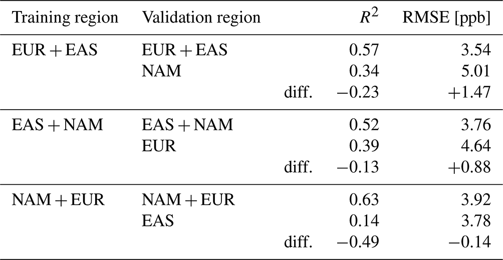
If our model is validated on a different region than it has been trained on, we observe a drop of the R² value by 0.13 to 0.49, while the RMSE increases for two of the three training regions (Table 5). One reason for the change in evaluation scores when training and validating in different world regions could be different feature combinations of the different world regions. We ruled out this reason by inspecting the feature space (similar to Sect. 2.3.1; not shown). The only other possible reason for the decrease in R² is that the relationship between features and ozone is not the same in different world regions. Therefore, the expected evaluation scores of our map vary not only with the feature combinations (as described in Sect. 2.3.1) but also spatially. We differentiate between the two issues and their influence on the model applicability in Sect. 3.2.1.

Table 4 Four-fold cross-validation results.

Table 5 Cross validation on the world regions Europe (EUR), East Asia (EAS), and North America (NAM). We give the difference in R² values and RMSEs when validating the model in another world region than the training region.

3.1.3 SHAP values quantify the influence of the features on the model results

SHAP was used to determine the feature importance of the random forest model as described in Sect. 2.2.4. Figure 5 contains a summary plot with the global feature importance (left side) and SHAP values of all features on the test set (right side). The global importance of the features “absolute latitude”, “altitude”, “relative altitude”, and “nightlight in 5 km area” are highest with a contribution of at least 10 %. The remaining features have a weaker influence on the model output. For example, the influence of the “climatic zone” is often negligible. The local SHAP values in Fig. 5 reveal the contribution of features to the predictions. A lower “absolute latitude” value leads to an increased ozone value prediction. Likewise, higher “altitude” and “relative altitude” increase predicted ozone values. High “nightlight in 5 km area” values lead to lower predicted ozone concentrations. These tendencies are in line with domain knowledge on the atmospheric chemistry of ozone. Appendix E shows SHAP values of two individual predictions. We discuss the physical consistency of the model based on the SHAP values in Sect. 4.1.

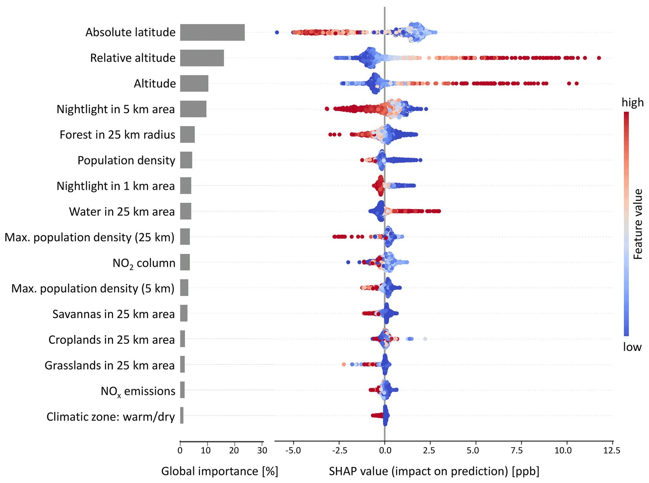
Figure 5 SHAP summary plot. The global importance on the left side is calculated from the averaged sum of the absolute SHAP values. The dots in the beeswarm plots on the right side show the SHAP values of single predictions. The color indicates the respective feature value. This plot shows only features with more than 1 % global importance.

3.2 Evaluating the impact of uncertainties

3.2.1 Applicability and uncertainty of the model depend on both features and location

As described in Sect. 2.3.1, predictions of our model are valid if the feature combinations are similar to those of the training dataset. Additionally, the results of the spatial cross validation (Sect. 3.1.2) have shown that the spatial proximity to the training locations has an influence on the model performance and uncertainty. Two cases were examined in this section: firstly, the cross-validation sets which are close to each other (RMSE in the range of 4 ppb, as seen in Table 4), and secondly, the cross validation on different world regions (RMSE values of up to 5 ppb, as seen in Table 5). In our uncertainty assessment, we therefore combine findings from both the area of applicability (for matching features) and the spatial cross-validation methods (for spatial proximity).

Analogously to the approach of the area of applicability (Sect. 3.2.1), we analyze the distances between measurement stations in the geographical space. To quantify spatial proximity, we calculate the mean distance of a measurement station and its closest neighboring station in a different cross-validation set. Disregarding stations that are too far away from the others, we identified the distance of approximately 182 km (upper whisker), within which we expect a comparable RMSE as shown in Table 4. We assume a higher RMSE for locations that are more than 182 km away from their closest neighboring measurement station. Figure 6 shows the area of applicability of our model including this spatial distinction.

The majority of the regions with good coverage of measurement stations (North America, Europe, and parts of East Asia) are well predictable. In these regions, only some areas in the high north and high mountains are not predictable. Conversely, large areas in South and Central America, Africa, far northern regions, and Oceania have feature combinations different from the training data and therefore are not predictable. There are some regions in the Baltic area, South America, Africa, and south Australia where feature combinations can be predicted by the model, but they are far away from the AQ-Bench stations. A broader discussion of the global applicability of our machine learning model follows in Sect. 4.3.

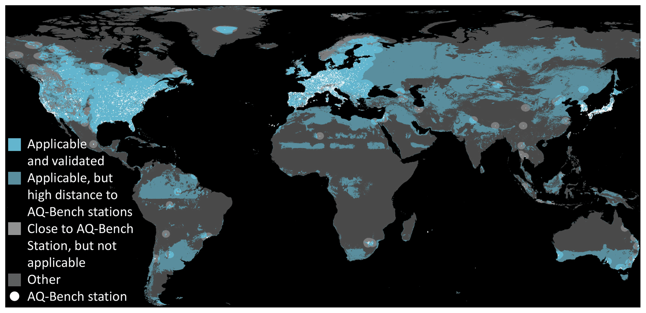
Figure 6 Area of applicability with restrictions in the feature space and spatial restrictions. The bright turquoise areas fulfill all prerequisites to be predictable: they have similar features as the AQ-Bench dataset and they are close to stations for validation. The darker shade of turquoise indicates similar predictions but no proximity to stations for validation. Light gray areas indicate the proximity of a station but no applicability of the model. The locations of all measurement stations are plotted in white.

3.2.2 Uncertainty due to ozone fluctuations is within an acceptable range

The error model for ozone uncertainties is described in Sect. 2.3.2. The R² values of the perturbed models varied between 0.50 and 0.58. Figure 7 shows the resulting standard deviation in the mapped ozone. The assumed ozone fluctuations have a higher impact in areas with sparse training data. We conclude that our error model does not tend to amplify the effects of perturbed training data. This means that the machine learning algorithm smoothes out noise during training. This is explained by the core functioning of the random forest which uses bootstrapping during training.

Figure 7 also shows that regions with poor spatial coverage by measurement stations (darker shade of turquoise in Fig. 6) are more sensitive to noisy training data. Example regions are the patches in Greenland, Africa, Australia, and South America. This is because the model relies its predictions on a few samples and is thus sensitive to perturbations of these few measurements.

Figure 7 Standard deviation of the ozone predictions under perturbations. This map was created by stacking the maps of 100 error model realizations along the z axis and then calculating the grid point-wise standard deviation along the z axis.

3.2.3 Uncertainty through subgrid DEM variation is within an acceptable range

This method was described in Sect. 2.3.3. In most regions of the world, subgrid DEM variations around mean altitude are below 50 m (Fig. 8a), e.g., in the central and eastern United States and in Europe except for the Alps. There are regions with higher variances such as the Rocky Mountains and their surroundings, the Alps, and large parts of Japan outside Tokyo. In Fig. 8b, it can be seen how these variations influence the predicted ozone values. In the flat regions, the variance is below 0.5 ppb, and even in the high-variance regions, the deviation is seldom above 2 ppb. This means the model is robust against these variances. Few exceptions are present at the border of the area of applicability (Sect. 3.2.1), e.g., in the Alps. But even in these regions, the deviation is well below 5 ppb. A discussion of implications for general subgrid variances can be found in Sect. 4.1.

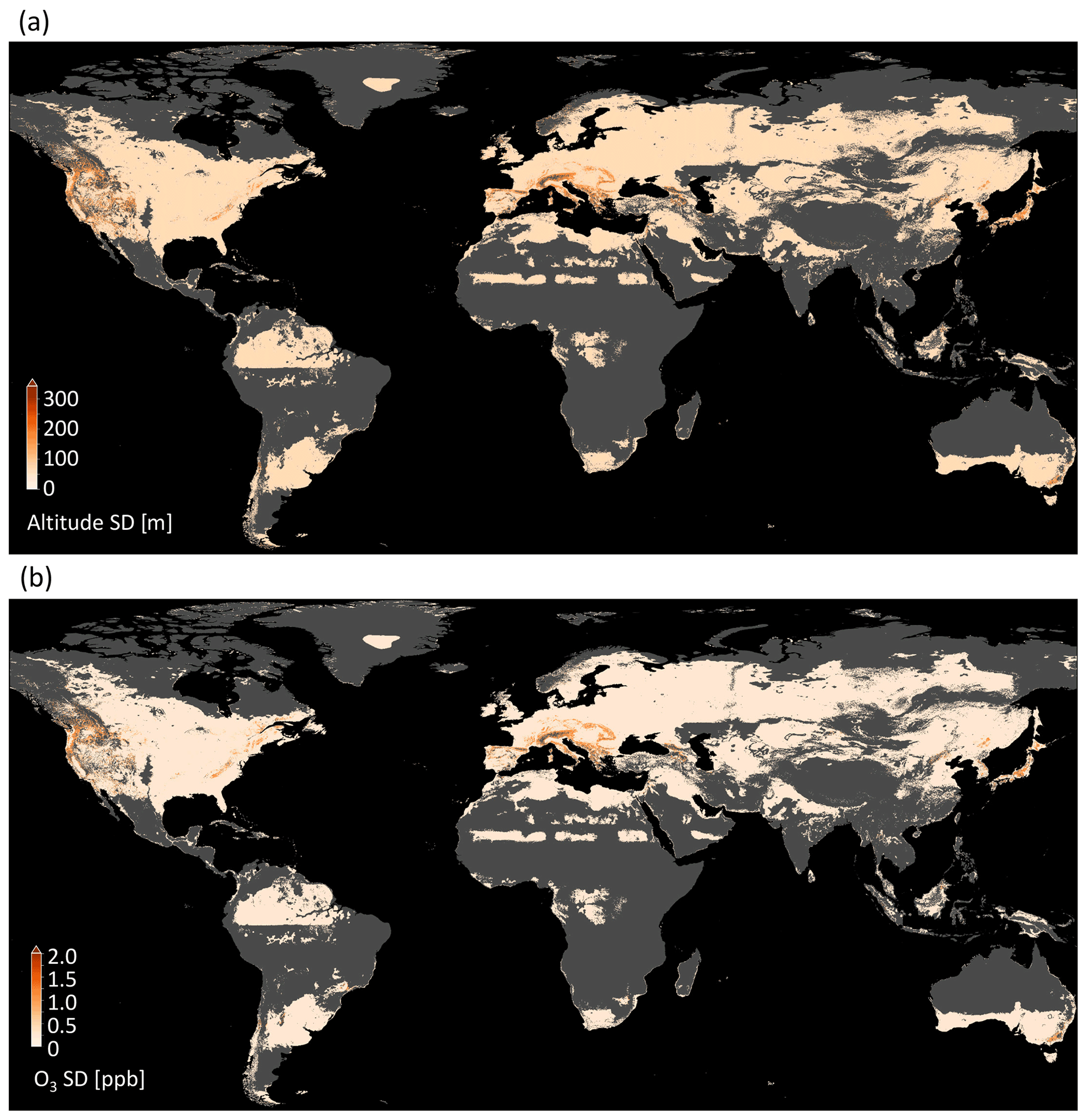
Figure 8 Results of propagating subgrid DEM variations through the model. (a) Spread of subgrid DEM data. (b) Spread of ozone values.

3.3 The final ozone map

3.3.1 Production of the final map

All selected features listed in Sect. 3.1.1 are used to fit the final model. In contrast to the experiments in the previous sections, we train the model on 80 % of the AQ-Bench dataset and test it on the remaining 20 % of the independent test set. Figure 2 shows the predictions on the test set vs. the true values. The R² value of this model is 0.55 and the RMSE is 4.4 ppb. There is a spread around the 1:1 line; furthermore, extremes are not captured as well as values closer to the mean. True values of less than 20 ppb or more than 40 ppb are predicted with high bias, which is expected since random forests tend to predict extremes less accurately than values closer to the mean.

3.3.2 Visual analysis

The final map is shown in Fig. 9 (data available under https://doi.org/10.23728/b2share.a05f33b5527f408a99faeaeea033fcdc, Betancourt et al., 2021d). Predictions are in a range between 9.4 and 56.5 ppb. There are some characteristics that are visible at first sight, e.g., higher values in mountain areas, like in the western US. The global importance of “absolute latitude” shows through a latitudinal stratification and a clear north–south gradient in Europe, the US, and East Asia. Sometimes the borders of climatic zones are visible, like in the north of North America, and across Asia. This shows that even if the climatic zones are not important globally, they can be locally important. There are larger areas with low ozone variation in Greenland, Africa, and South America.

In Fig. 10, a detailed look at three selected areas is given, and the predictions are compared to the true values. In Fig. 10a, a uniform, low ozone concentration is predicted over the peninsula of Florida. Figure 10b shows low ozone values in the Po Valley, a densely populated plane. Towards the mountains which surround the valley, higher values are predicted, and for the higher mountains, no predictions can be made. Figure 10c shows the city of Tokyo, which is covered with ozone measurements and where ozone values are relatively low. At the coasts of Japan, the values are lower. The spatial ozone patterns described here can also be found in ozone maps generated by traditional chemical models such as the fusion products by DeLang et al. (2021). We discuss the prospects of global ozone mapping more thoroughly in Sect. 4.4.

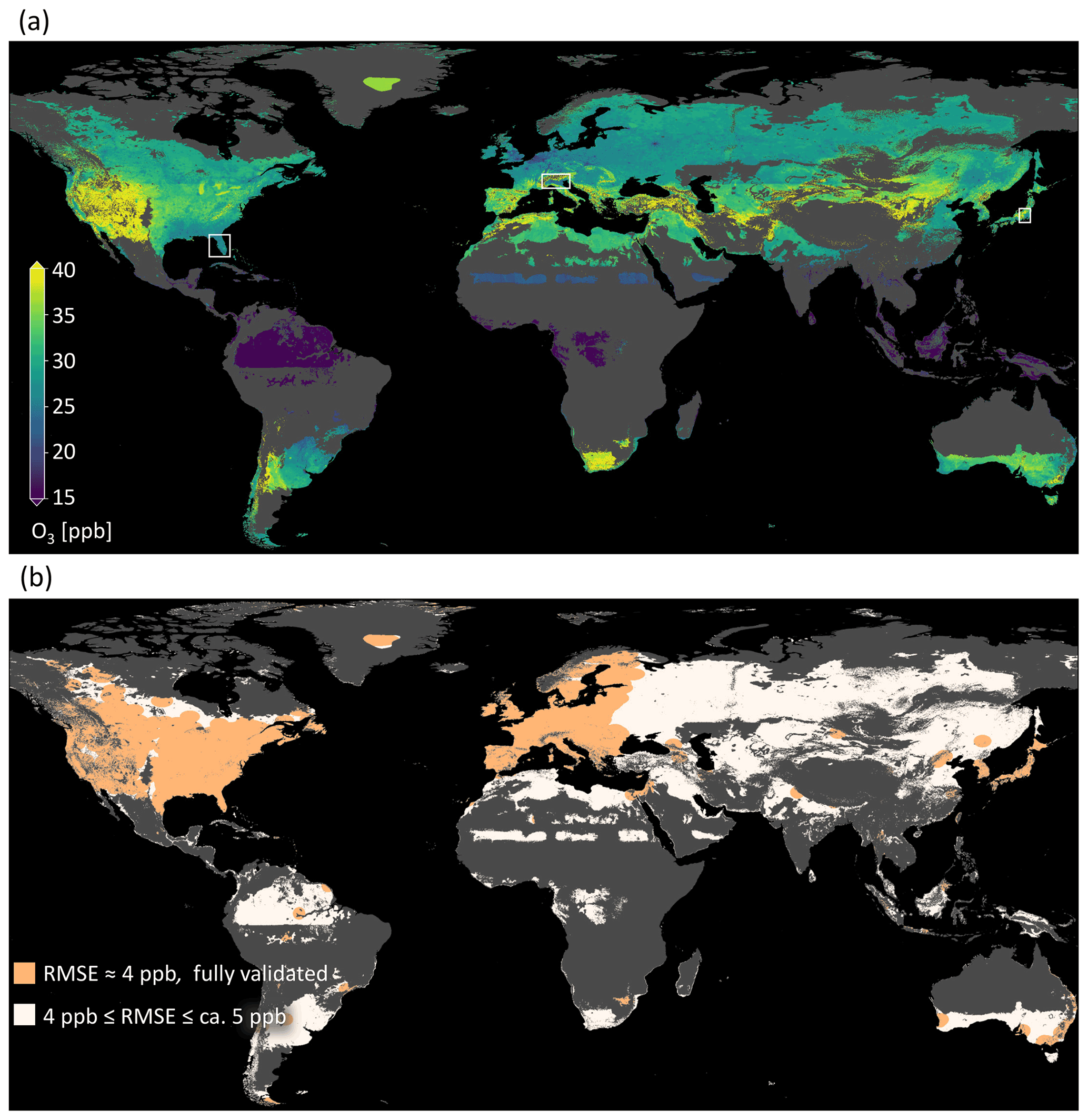
Figure 9 The final ozone map as produced in this study. Panel (a) shows the ozone values; (b) shows the uncertainty estimates. The areas shown in Fig. 10 are highlighted by white boxes.

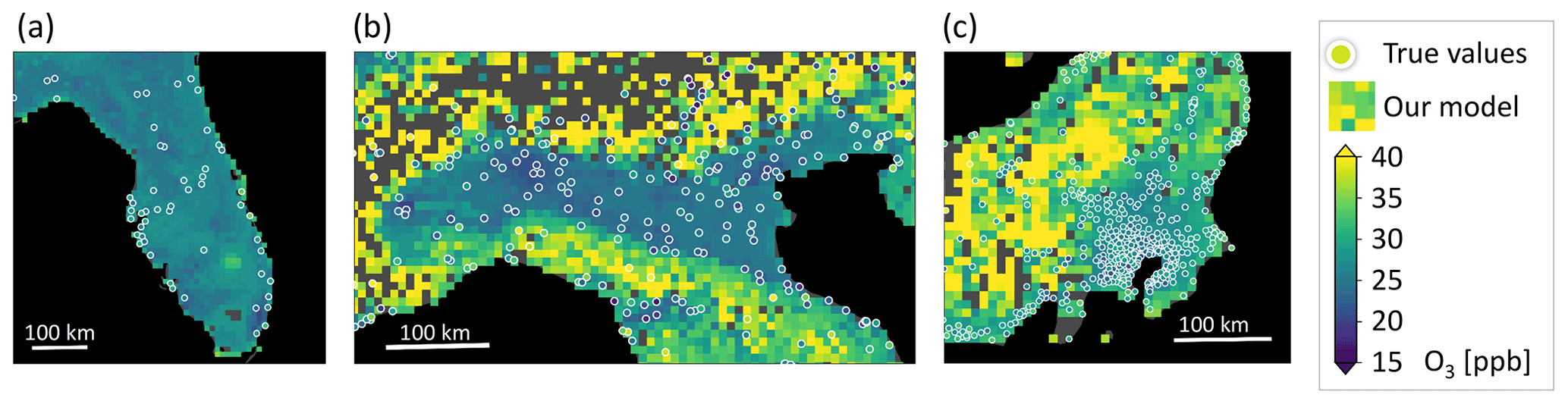
Figure 10 Map details with true values are given as white circles. (a) The Florida peninsula, USA. (b) The Po Valley in northern Italy. (c) Tokyo, Japan, and its surroundings.

4 Discussion

4.1 Robustness

Based on Hamon et al. (2020), we define robustness as follows: The model and map are considered robust if they do not change substantially under noise or perturbations that could realistically occur. We define a 5 ppb change in RMSE score or predicted ozone values as significant (Schultz et al., 2017). Methods to assess the robustness are part of both the explainable machine learning workflow (Table 2) and the uncertainty assessments (Table 3). Regarding the robustness of the training process, the cross-validation results in Table 4 show that the model performance depended on the data split. This was already noted by Betancourt et al. (2021b) and is regarded as an inherent limitation of a noisy dataset.

We tested the robustness regarding typical variances in the ozone and geospatial data. The results from Sect. 3.2.2 and 3.2.3 show that the produced ozone map is robust against these fluctuations. The variances are never above the initial perturbations, and variances in the map do not exceed our limit of 5 ppb. Limits in the robustness were only shown through variances above 3 ppb at the borders of the area of applicability, and in regions with sparse training data (gray and dark turquoise areas in Figs. 7 and 8). This outcome shows that the issues of applicability (Sect. 4.3) and robustness are interconnected. In areas where the model is applicable, it is also more robust and uncertainties are lower.

In order to make the robustness assessment with respect to data feasible, we strongly reduced the dimensionality of our error model by using expert knowledge. We conducted two experiments where we modify training data and model inputs (Sect. 2.3.2 and 2.3.3). These experimental setups were chosen because they are expected to generalize well. The combined robustness experiments have shown that our produced maps are robust.

4.2 Scientific consistency

We discuss the scientific consistency of our model by assessing the results of the explainable machine learning workflow (Table 2). We interpret the selected features, their importance, and their influence on the model predictions. The features are proxies to ozone processes, which makes it challenging to interpret the underlying chemical processes. Nevertheless, the connections between the features can be discussed, if they are plausible and consistent with respect to our understanding of ozone processes. This is a pure a posteriori approach, meaning we did not in any way enforce scientific consistency during the training process.

Regarding the global feature importance of SHAP (Fig. 5), it might be counterintuitive that the model focuses more on geographical features such as “absolute latitude” and “altitude” than chemical factors such as the “NO₂ column”, and “NO_x emissions”. Geographic features are proxies for flow patterns and heat, not for ozone chemistry, which would be expected to be more important. This contradiction is due to the fact that the model provides an as-is view of ozone concentration and is not process oriented in any way. Many features such as “nightlight” and “population density” are correlated, so retraining the model might swap dependence in the SHAP values as noted by Lundberg et al. (2020).

The beeswarm plot in Fig. 5 shows the physical consistency of our model. The effect of “absolute latitude” on predictions is consistent with known ozone formation processes; i.e., ozone production generally increases when more sunlight is available. This is also evident in the latitudinally stratified ozone overview plots in global measurement-based studies such as TOAR health and TOAR vegetation (Fleming et al., 2018; Mills et al., 2018). Ozone is affected by meteorology (temperature, radiation) and precursor emissions (Sect. 1). The fact that there is no continuous increase of ozone towards tropical latitudes shows that the mapping model at least qualitatively captures the influence of low precursor emissions in the tropics. The importance of “absolute latitude” also indicates that the model can be improved by including temperature and radiation features from meteorological data. High “relative altitude” and “altitude” both increase the predicted ozone. These relations are consistent with Chevalier et al. (2007). There are relatively important chemistry-related features. We see that high values of “nightlight in 5 km area” reduce the predicted ozone. This is consistent with NO titration (Monks et al., 2015). Nightlights are a proxy for human activity, generally in the context of fossil fuel combustion, which leads to elevated NO_x concentrations. NO destroys ozone, and especially during the night time this leads to ozone levels close to zero ppb. High “forests in 25 km area” values lead to lower ozone predictions. This is plausible because there is little human activity in forested areas and thus no combustion-related precursor emissions occur. Quantification of either influence is not possible because, for example, it is unclear to what extent the different forests emit volatile organic compounds which are also ozone precursors. A city with “nightlight in 5 km area” equal to 50 cannot be directly quantified in terms of precursor emissions either. It is also not expected that the machine learning model learns the ozone-related processes described above because it is not process based. Instead, it learns the effects of processes if they are reflected in the training data.

The forward feature selection (Sects. 2.2.2 and 3.1.1) can also be discussed in terms of plausibility. Features selected by this method favor a generalizable model. Discarded features may help to characterize the locations, but their addition to the training data does not lead to a more generalizable model. “Urban and built-up in 25 km area” was not selected presumably because urban areas are often localized. This feature is therefore not as meaningful as the variables “nightlight” and “population density”, which are also proxies for human activity, but are available at higher resolution. Similarly, the feature “cropland/natural vegetation mosaic in 25 km area” was discarded because ozone is affected differently by croplands and natural vegetation. Together with the large area considered, this feature becomes obsolete. We suspect the features “snow and ice in 25 km area”, “barren or sparsely vegetated in 25 km area”, and “wheat production” did not contribute to the model generalizability because they are simply not represented well in the training data. A feature may be an important proxy for ozone, but if the relationship is not expressed in the training data, it cannot be learned by a machine learning model. This feature can become more important if other training locations are included. This shows that the placing of measurement locations is crucial.

4.3 Mapping the global domain

The model has to generalize to unseen locations for global mapping. Two prerequisites are (1) the model must have seen the feature combination during training; (2) the connection between features and the target, ozone, must be the same. The two conditions are only fulfilled in a strictly constrained space, as shown in Fig. 6. We combined cross validation with an inspection of the feature space to ensure matching feature combinations. Then, based on the cross validation on different world regions, we point out regions with sparse or no training data, where higher model errors are expected (Sect. 3.2.1). We also conducted spatial cross validation with a shallow neural network (as in the baseline experiments of Betancourt et al., 2021b). The neural network had similar evaluation scores on the test set but did not generalize to other world regions, even showing negative R² values when evaluated in other world regions. We decided to discard the neural network architecture, because our main goal is global generalizability.

We can confidently map Europe, large parts of the US and East Asia, where the majority of the measurement stations are located. Those are industrialized countries in the northern hemisphere. The cross-validation results (Sect. 3.1.2), the area of applicability (Sect. 3.2.1), and expert knowledge confirm that uncertainties increase when a model trained on the AQ-Bench dataset is applied to other world regions. However, the cross validation in connection with the area of applicability technique shows that the model can be used in other world regions with acceptable uncertainties. That is promising for future global mapping approaches. One idea to solve these problems of different connections between features and ozone in different world regions is to train localized models, and apply them wherever possible. Localized models could not only yield more accurate predictions but in connection with SHAP values (Sect. 2.2.4), they could also rule out the governing factors of ozone in the respective regions and be easier to interpret.

With regard to the spatial domain, we can also discuss the resolution. The model was trained on point data of the “absolute latitude”, “altitude”, and “relative altitude”, and one could produce more fine-grained maps if the gridded data are present in higher resolution. However, one may need to reconsider some assumptions made here in terms of regional representativity of the measurements and the relation between geographic features and ozone on a different scale.

4.4 Prospects for ozone mapping

We mapped average tropospheric ozone from the stations in the AQ-Bench dataset to a global domain. For this, we fused different auxiliary geospatial datasets and gridded data with machine learning. We used features that are known proxies for ozone processes, and that were already proven to enable a prediction of ozone concentrations (Betancourt et al., 2021b). Our choice of data and algorithms is well justified and transparent. Errors did not exceed 5 ppb, which is an acceptable uncertainty. The R² value of the final model is 0.55, which is a good value for properly validated mapping. The maps produced show known patterns of ozone such as lower levels in metropolitan areas and higher levels in Mediterranean or mountainous regions. However, extremes (Fig. 2) are predicted with higher bias. This can be considered as a general problem of machine learning (Guth and Sapsis, 2019) but was also noted in other ozone modeling studies (Young et al., 2018).

For this first approach, we limited ourselves to the static mapping of aggregated mean ozone. An advantage of this approach is that the model result is directly the ozone metric of interest (in this case, average ozone). Since the AQ-Bench dataset contains other ozone metrics, they could be mapped as well. For example, vegetation- or health-related ozone metrics can be mapped with the same workflow as described here. Another advantage is that we used a multitude of inputs that could not be used in a traditional model because their connection to ozone is unknown. This means we exploit two benefits of machine learning: first, obtaining a bias-free estimate of the target directly, and second, using a multitude of inputs with unknown direct impact on the target.

Our model is only valid for the training data period (2010–2014), and it is not suitable to predict ozone values in other years. Our data product is a map that is aggregated in time. This could be a limitation as sometimes the data product of interest is a seasonal aggregate or even maps of daily or hourly air pollutant concentrations. The use of meteorological data as static or non-static inputs can be beneficial to further increase model performance and allow time-resolved mapping. We applied a completely data-driven approach, relying heavily on geospatial data. The other side of the spectrum is DeLang et al. (2021), who fused chemical transport model output to observations without exploiting the connection to other features. A possible direction to go from here is described by Irrgang et al. (2021), who propose the fusion of models and machine learning to benefit from both methods.

5 Conclusions

In this study, we developed a completely data-driven, machine-learning-based global mapping approach for tropospheric ozone. We mapped from the 5577 irregularly placed measurement stations of the AQ-Bench dataset (Betancourt et al., 2021b) to a regular 0.1^∘ × 0.1^∘ grid. We used a multitude of geospatial datasets as input features. To our knowledge, this is the first completely data-driven approach to global ozone mapping. We combined this mapping with an end-to-end approach for explainable machine learning and uncertainty estimation. This allowed us to assess the robustness, scientific consistency, and global applicability of the model. We linked interpretation tools with domain knowledge to obtain application-specific explanations, which is in line with Roscher et al. (2020). The methods are interconnected; e.g., forward feature selection made the model easier to interpret. Likewise, the area of applicability was shown to match the model's robustness. We justified the choice of tools and detailed how they provided us with the results to make a comprehensive global analysis. The combination of explainable machine learning and uncertainty quantification makes the model and outputs trustworthy. Therefore, the map we produced provides information on global ozone distribution and is a transparent and reliable data product.

We explained the outcome and the model, which can lead to new scientific insights. Mapping studies like ours could also contribute to studies like Sofen et al. (2016) that propose locations for new air quality measurement sites to extend the observation network. Here, the inspection of the feature space helps to cover not only spatial world regions but also air quality regimes and areas with diverse geographic characteristics. Building locations can also be proposed based on their contribution to maximizing the area of applicability (Stadtler et al., 2022). The map as a data product can also be used to refine studies like TOAR (Fleming et al., 2018; Mills et al., 2018) because it enables analyzing locations with no measurement stations.

It would be beneficial to add time-resolved input features to the training data to improve evaluation scores and increase the temporal resolution of the map. Adding training data from regions like East Asia, or new data sources such as OpenAQ (https://openaq.org/, last access: 2 November 2021), would close the gaps in the global ozone map.

Appendix A: Technical details on the data

Betancourt et al. (2021b)Schultz et al. (2017)Schultz et al. (2017)Schultz et al. (2017)Amante and Eakins (2009)Amante and Eakins (2009)Janssens-Maenhout et al. (2015)Krotkov et al. (2016)CIESIN (2005)

Table A1 Technical details on the data used in this work. For more information on the station location data, refer to Betancourt et al. (2021b). Please note that “land use in 25 km area” comprises all the different land cover features.

Appendix B: Plots of gridded fields used as inputs for mapping model

Figure B1 Gridded fields used for the final map production. Please note that the feature engineering was done as described in Sect. 2.2.2.

Figure B2 Gridded fields used for the final map production. Please note that the feature engineering was done as described in Sect. 2.2.2.

Appendix C: Example realization of error model

Figure C1 Example realization of the error model for ozone uncertainties as described in Sect. 2.3.2. A random subset of 25 % of the ozone values in the training set is perturbed with values sampled from a Gaussian distribution with 0 ppb mean and 5 ppb variance.

Appendix D: Convergence of the error model

Figure D1 This plot justifies the use of 100 error model realizations in Sect. 3.2.2. We have stacked n perturbed maps along the z axis and monitored the grid point wise standard deviation along the z axis. The mean standard deviation over the whole map stabilizes after approximately 40 realizations. The maximum standard deviation exceeds 3.5 ppb for less than 20 realizations. This can be explained by the fact that some grid points base their predictions on single, differently perturbed stations when the number of realizations is low. This effect smoothes out after 20 realizations. Even though the maximum is not as stable as the mean (which is expected), convergence can be assumed after 100 realizations.

Appendix E: SHAP values of single predictions

Figure E1 SHAP force plots for two example low-bias (< 1 ppb) predictions at (a) a rural station in the US and (b) an urban station in France, in addition to SHAP results from Sect. 3.1.3. Starting from the base value (27.7 ppb), a feature can increase or decrease the predicted ozone (red and blue arrows). The final predictions (23.5 and 31.9 ppb, respectively) result from adding all SHAP values to the base value. The most contributing features are labeled and their values are given. The high ozone station (a) is located in a rural area in the US with many agricultural fields and a smaller city nearby. The average ozone at this location is predicted to be high because the model uses the absence of forests, the low “nightlight in 5 km area” value, and the “absolute latitude” as features leading to high ozone values. This is consistent with Fig. 5, where it can be seen that a lower “absolute latitude” often increases the ozone value. The French station (b) is an urban background station surrounded by fields. The location is further in the north than the US station which leads to a strong decrease in the predicted ozone value. The low “(relative) altitude” further decreases the predicted ozone.