Modeling subgrid lake energy balance in ORCHIDEE terrestrial scheme using the FLake lake model

The freshwater 1-D FLake lake model was coupled to the ORCHIDEE land surface model to simulate lake energy balance at the global scale. A multi-tile approach has been chosen to allow the modeling of various types of lakes within the ORCHIDEE grid cell. Thus, three different lake tiles have been defined according to lake depth which is the most influential parameter of FLake, but other properties could be considered in the future. Several depth parameterization strategies have been compared, differing by the way to aggregate the depth of the subgrid lakes, i.e., arithmetical, geometrical, harmonical mean and median. Five atmospheric reanalysis datasets available at 0.5^∘ or 0.25^∘ resolution have been used to force the model and assess model systematic errors. Simulations have been performed, evaluated and intercompared against observations of lake water surface temperatures provided by the GloboLakes database over about 1000 lakes and ice phenology derived from the Global Lake and River Ice Phenology database.

The results highlighted the large impact of the atmospheric forcing on the lake energy budget simulations and the improvements brought by the highest resolution products (ERA5 and E2OFD). The median of the root square mean errors (RMSEs) calculated at global scale ranges between 3.2 and 2.7 ^∘C among the forcings, CRUJRA and ERA5 leading respectively to the worst and best results. The depth parameterization strategy appeared to be less influential, with RMSE differences less than 0.1 ^∘C for the four aggregation scenarios tested.

The simulation of ice phenology presented systematic errors whatever the forcing and the depth parameterization used. Large systematic errors were highlighted such as negative biases on the onset and positive biases on the offset. Freezing onset was shown to be the less sensitive to atmospheric forcing with the median of the errors ranging between 10 and 14 d. Larger errors up to 25 d were observed on the simulation of the end of the freezing period. Such errors, already highlighted in previous works, could be explained by scale effects and deficiencies in the modeling of snow–ice processes not accounting for partial ice cover. Various pathways are drawn to improve the model results, including the use of remote sensing data to better constrain the lake radiative parameters (albedo and extinction coefficient) as well as the lake depth thanks to the recent and forthcoming high-resolution satellite missions.

1 Introduction

Lakes are an important component of the continental hydrology and interfere in the global carbon cycle. Lakes do play a role in many physical and biogeochemical processes at the land–atmosphere interface such as the transfers of energy, water, carbon and other greenhouse gases (GHGs) like methane. However, since they represent only a small percentage of the land surface (about 3.7 % as shown by Verpoorter et al., 2014), their contribution at the global scale is small (at least regarding the energy and water budgets). Therefore, lakes started to be explicitly represented in Earth system models (ESMs) only recently, thanks to the increased grid resolutions and computer advances.

Lake distribution is spatially unequal all around the world with two regions in the high latitudes (Canada and Scandinavia) showing the highest number of lakes (Downing et al., 2006). The second characteristic of this distribution is the presence of large lakes in northern America and Africa which represent 27 % of the world's total lake water volume and 11 % of the lake surface (Messager et al., 2016). Their role in the physical properties of the low atmosphere as well as the importance of modeling these processes has been demonstrated by many studies. For example, Bonan (1995) showed that the implementation of lakes in the NCAR-CCM2 climate model leads to an increase in the latent heat fluxes transferred to the atmosphere and to a decrease in the annual amplitude of the surface temperature. They found that in the high inland lake regions in July, the average lake surface temperature was cooler by 2 to 3 ^∘C and that the latent heat fluxes increased by 10 to 45 W m⁻² depending on the region.

Lakes also play a buffer role in the hydrological cycle substantially impacting the river regimes. As an example, in Alaska, Bowling and Lettenmaier (2010) explain the reduction of the spring peak flow of the Putuligayuk river by the lake storage, which represents up to 80 % of the snowmelt.

Regarding the carbon and nitrogen cycles, lake emissions are poorly constrained, but it is recognized that their contribution is significant (Bastviken et al., 2004). Lakes are a carbon source for the atmosphere, with CO₂ emissions of about 110 Tg C in annual mean, but they are also a sink since an important part of organic carbon is buried into the bottom sediments (Cole et al., 2007). Another important GHG is the methane generated from methanogenesis by micro-organisms in anaerobic conditions, processes which are presently poorly understood but could lead to lake emissions between 8 and 48 Tg C-CH₄ yr⁻¹, comparable to the emissions of the oceans (Bastviken et al., 2004). For example, West et al. (2016) estimated that between 8 % and 16 % of the non-anthropic methane emissions are coming from lakes. Recently, Beaulieu et al. (2019) gave a higher estimation of lake methane emissions with an amount of 112 Tg C-CH₄ yr⁻¹.

Given the role of lakes in the global carbon and water cycles, the large uncertainties related to GHG budgets (Saunois et al., 2020) and the increasing spatial resolution of ESMs allowing the land surface diversity to be better accounted for, it becomes necessary to implement water bodies in ESMs. At the scale of the ESMs (typically a few hundred of kilometers), lakes can not be explicitly represented and have to be aggregated in water fractions with effective parameters, allowing the surface energy balance to be solved and the prediction of the time evolution of the surface temperature and fluxes exchanged with the atmosphere. Among all the models developed for that purpose, the one-dimensional approaches are the most used in ESMs because of their low computational cost and the robustness of the parameterizations based on a few number of free parameters. In this category, the FLake model (Mironov, 2008) and the Hostleter model (Hostetler and Bartlein, 1990) are the most used to represent lakes in ESMs. These two models follow different approaches to solve the lake energy budget and to calculate the energy vertical transfers and the water temperature profile: in FLake, the temperature profile is computed through the self-similarity theory, whereas in Hostleter’s model, the eddy diffusive equations are explicitly resolved. An intermediate methodology resolving the turbulence in the mixing layer with a bulk approach was used by MacKay (2012) in the Canadian Small Lake Model (CSLM). This model was successfully implemented in the Environment and Climate Change Canada's surface prediction system (Garnaud et al., 2022). All these methods have shown good performances when compared at site level and participated in various intercomparison exercises. For example, in LakeMIP, Stepanenko et al. (2010, 2013) showed the good performances of a number of these models in predicting the water surface temperature and fluxes of various types of lakes.

As such, FLake has been implemented in numerous climate and numerical weather prediction models. For example, it has been coupled to the German regional atmospheric model (COSMO) and its TERRA land component (Mironov et al., 2010), the European Centre for Medium-Range Weather Forecasts (ECMWF) atmospheric model and its HTESSEL land surface component (Balsamo et al., 2012; Dutra et al., 2010), and the French CNRM-CM5 ESM and its SURFEX interface (Le Moigne et al., 2016). Flake is also part of the JULES Land simulator (Rooney and Bornemann, 2013) of the UK Met Office Unified Model and can be run in a stand-alone version. The coupling of FLake with all these LSMs showed strong benefits in the climate and weather simulations. In addition, the LISSS (Subin et al., 2012) model based on the Hostetler model is used in the CLM land component of the CESM climate model developed by the NCAR institute (Oleson et al., 2013) and in the land models BCC-AVIM (Golaz et al., 2019) and NorESM2 (Seland et al., 2020). The LISSS model is also implemented in the LM4 land component of the Geophysical Fluid Dynamics Laboratory’s ESM (Milly et al., 2014) and in the land component CLASS of the Canadian ESM (Martynov et al., 2012). More recently, mass balance equations have been implemented in some ESMs in order to solve the coupled energy and water cycles. For example, Huziy and Sushama (2017) implemented a lake mass budget in the CLASS LSM and tested it for regional applications. As well as this, Guinaldo et al. (2021) developed the MLake mass budget model in SURFEX environment, thus enabling the improvement of the global-scale water discharges and the seasonal evolution of lakes water levels.

This study aims to include lakes in the ESM of the Institut Pierre Simon Laplace (IPSL) and more precisely in its land surface component ORCHIDEE. Contrary to Krinner (2003) who directly introduced the Hostetler model in its atmospheric model component (LMDZ) and in this way highlighted the role of water surfaces in the boreal climate, we chose here to explicitly represent the lakes in ORCHIDEE and to resolve, as a first step, the energy balance. For that purpose, the FLake lake model was coupled to ORCHIDEE and various developments were made to represent lakes in the grid cell, define effective parameters and set up the new parameterizations. We present these developments here and the results obtained through a series of simulations devoted to assessing the respective role of the atmospheric forcing and of depth parameterization in the model performances. We focus on the analysis of the simulated surface variables (temperature, freezing state and turbulent fluxes) which are impacting the atmospheric surface boundary layer. Model performances are analyzed at the lake scale and globally against satellite datasets. The contribution of lakes in the simulation of the surface temperature and energy fluxes is quantified. The following steps including further model developments and parameter optimization are finally discussed.

2 Data and modeling framework

2.1 Datasets used

2.1.1 Land cover map

The Land Cover CCI product (v2.0.7, Bontemps et al., 2015, ESA, 2017) developed in the framework of the Climate Change Initiative program of the European Space Agency (ESA) is used as a standard in ORCHIDEE to map the natural vegetation and derive the plant functional types (PFTs) describing the subgrid variability of the vegetation. The product is available at a resolution of 300 m and the global maps are provided on a yearly basis, over the period 1992–2020. The interpretation of the 38 land cover classes in terms of ORCHIDEE PFTs is fully presented in Poulter et al. (2015) and Hartley et al. (2017) and detailed in the dedicated website https://orchidas.lsce.ipsl.fr/dev/lccci (last access: 19 May 2022​​​​​​​). In this work, we used the PFT maps generated at the resolution of 0.25 and 0.5^∘ for the standard version of ORCHIDEE.

2.1.2 Lake area and depth

The HydroLAKES database (Messager et al., 2016) has been used to characterize lake fractions and depths. The dataset provides georeferenced polygons for 1.4 million lakes of size larger than ​​​​​​​0.1 km². A mean depth is provided for each water body, estimated either from in situ measurements or from geomorphological considerations allowing assessment of lake shape from which depth is derived. Additional attributes include estimates of the shoreline length, water volume and residence time, but they were not used in this work. Moreover, all lakes are co-registered to the global river network of the HydroSHEDS database used in ORCHIDEE to describe the river system and constrain the water routing scheme. This specificity will then insure the coherence for the next developments around the modeling of the water budgets and the lake–river interactions. The data can be downloaded at https://hydrosheds.org/page/hydrolakes (last access: 19 May 2022​​​​​​​).

2.1.3 Lake surface temperatures

The Global Observatory of Lake Responses to Environmental Change (GloboLakes) database is used to evaluate our simulations. This dataset has been developed thanks to a project funded by the UK Natural Environment Research Council in the continuity of the ARC-Lake database (MacCallum and Merchant, 2012) funded by the European Space Agency. It provides daily observations of lake surface water temperature (LSWT) for about 1000 lakes distributed all around the world, with uncertainties and quality level. The observations cover the period 1995–2016 with a spatial resolution of 0.05^∘ and combine different instruments such as the AVHRR (Advanced Very High Resolution Radiometer) on MetOpA, AATSR (Advanced Along Track Scanning Radiometer) on Envisat and ATSR-1/2 (Along Track Scanning Radiometer) on ERS-1/2 (European Remote Sensing Satellite) covering different periods. The time series from ATSR-2 are available for the period 1995–2002, from AATSR for the period 2002–2010 and from AVHRR for the period 2007–2016. A common processing methodology as well as the fact that all the satellites have a quasi polar orbit leading to a constant local solar time allowed a time homogeneity in the measurements and a homogeneous resulting dataset (Carrea and Merchant, 2019). Given the lack and lower quality of the data before 2002 due to the older instruments, we used the reduced period 2000–2016 for the model evaluation. For the whole period between 1995 and 2009 and for the previous version of the database ARC-Lake, the product uncertainty estimated by Carrea and Merchant (2019) is less than 1 ^∘C. The comparison against local measurements shows that errors are slightly larger for daytime measurements (0.7 ^∘C) compared to nighttime (0.5 ^∘C) with a small negative bias (−0.2 ^∘C during daytime and −0.1 ^∘C at night) linked to the thermal skin cooling effect. The data can be found at http://dx.doi.org/10.5285/76a29c5b55204b66a40308fc2ba9cdb3 (Carrea and Merchant, 2019)​​​​​​​.

2.1.4 Lake ice phenology

The Global Lake and River Ice Phenology Database is used to validate the lake freezing processes. This dataset provides the start, end and duration of the freezing period for 857 lakes located in the northern latitudes. The dataset is based on in situ measurements, which are sometimes discontinuous and acquired over different periods, and reports the dates of full ice coverage. The data are available for some lakes back to the year 1850 updated to 2020 (Benson et al., 2000). The data can be downloaded at https://doi.org/10.7265/N5W66HP8.

2.1.5 Atmospheric forcings

Different atmospheric reanalyses were used in this work to force the ORCHIDEE model and assess the model sensitivity to meteorological forcing uncertainties. These reanalysis differ by the model and data used to constrain the atmospheric fields, differences that may introduce some biases. Here, we used five different datasets available at three different spatial resolutions: 31 km, 0.25 and 0.5^∘ and three different temporal resolutions, hourly, 3-hourly and 6-hourly.

Then, for the simulations performed at 0.5^∘ resolution, we used the following forcing datasets: (a) WFDEI-CRU, a 3-hourly 0.5^∘ global forcing product which is a combination of the ERA-Interim reanalysis and the Climate Research Unit (CRU)-TS 3.1 climatological data (Harris et al., 2014) presented by Weedon et al. (2011); (b) CRUJRA, a 6-hourly 0.5^∘ global forcing product, which is based on JRA-55 reanalysis (Kobayashi et al., 2015) corrected by CRU-TS 3.2 (Harris et al., 2014); and finally (c) CRUNCEP, a 6-hourly 0.5^∘ global forcing product, which is a combination of two datasets, the CRU-TS 3.2 and the National Center for Environmental Prediction (NCEP) reanalysis product described by Viovy (2018). ERA5 (Hersbach et al., 2020), an hourly global forcing product at a resolution of 31 km, and E2OFD (Beck et al., 2017), a 3-hourly 0.25^∘ global forcing product complete the selection. All the data have been formatted by the ORCHIDEE team to be used and interpolated at the half-hourly time step, following the methodology presented in Wei et al. (2014) and summarized in https://forge.ipsl.jussieu.fr/orchidee/wiki/Documentation/Forcings (last access: 19 May 2022​​​​​​​). In brief, the interpolation of the meteorological variables is done linearly except for the solar radiation, where the interpolation between two time steps of the atmospheric forcing, follows a typical sinusoidal daily evolution according to the solar zenithal angle. It should be noted that no extra atmospheric fields are needed to solve the energy balance at the lake–atmosphere interface compared to what is done for the vegetated fraction of the grid.

2.2 Modeling framework

2.2.1 ORCHIDEE land surface model

ORCHIDEE is the land surface component of the IPSL ESM. It simulates the surface energy balance and the water, carbon and nitrogen cycles for large-scale and climate applications. The model is composed of two main modules named SECHIBA and STOMATE. SECHIBA resolves the thermal and hydrological processes at a half-hourly time step and computes the key surface variables and fluxes such as the soil temperatures (Wang et al., 2016) and water content (de Rosnay, 2003) with an 11-layer discretization, the evolution of the snow cover with an explicit 3-layer representation (Wang et al., 2013), and the photosynthesis of the vegetation (Vuichard et al., 2019). The second module STOMATE computes with a daily time step and the fully coupled carbon and nitrogen dynamics and therefore calculates key processes such as the vegetation respiration, the soil carbon dynamics, the litter decomposition and the vegetation phenology, constrained by the nutrients availability (Vuichard et al., 2019). The model can be run in forced mode with atmospheric variables prescribed or coupled with the atmosphere simulated by the atmospheric general circulation model LMDZ (Cheruy et al., 2020). In ORCHIDEE, the land surface is represented by two surface functional types (SFTs) differentiating bare and vegetated surfaces from glaciers. The first SFT allows the land surface to be represented in fractions of 15 different broad PFTs merging both plant species and main climate zones, one of them representing bare soils. In the standard version of ORCHIDEE, urban areas and water surfaces are not represented explicitly and are considered as bare soils. The fractions of PFTs assigned in a grid cell are determined by a land cover map and a cross-walking table (CWT) allowing the land cover classes to be linked to the ORCHIDEE PFTs. This procedure is fully presented in Lurton et al. (2020). The model can be used at various scales, from the local to the global scale, with grid resolutions constrained by the scale of the atmospheric input fields (incoming shortwave and longwave radiations, surface air temperature and humidity, wind speed and precipitation). In this work, the model version used is the AR6 version, which participated in the CMIP6 model intercomparison exercise and contributed to the IPCC 6th Assessment Report (Boucher et al., 2020; Cheruy et al., 2020).

2.2.2 FLake lake model

FLake (Mironov, 2008) is a 1-D thermodynamic lake model primarily developed for weather forecast modeling purposes. It is a bulk model capable of predicting the vertical temperature structure and mixing conditions in lakes, given the meteorological conditions at the atmosphere interface (incoming radiation, air temperature and humidity, wind speed, snowfall). The water temperature profile is represented by a single mixed layer with a uniform temperature above a thermocline. Extra modules are implemented to model the snow, ice and sediment profile temperatures into specific layers.

The structure of the lake thermocline is parameterized using the concept of self-similarity. Therefore, the depth–temperature relationship depends on a shape factor, which is resolved at each time step according to the boundary conditions. The same approach of “assumed shape” is used to represent the snow, ice and sediment layer temperature profiles.

The resolution of the bulk energy budgets of the mixed layer and thermocline allows the model prognostic variables to be calculated, i.e., the mixed-layer temperature and depth, the water bottom temperature, the thermocline shape factor, the ice layer top temperature, and ice thickness.

If the snow module is activated, the snow temperature at the atmosphere interface and the snow depth are calculated through an evolution equation that considers the snow precipitation rate within the time step. It should be noted that the model only resolves the energy budget equations and not the water balance. That means that the water volume is kept constant in time. The depth is therefore an input parameter of the model. In addition, two important radiative parameters, surface albedo and light extinction coefficient, as well as the surface fetch involved in the calculation of the surface fluxes need to be prescribed to run the model.

FLake does not model the hypolimnion, the layer under the thermocline which is present or may appear seasonally in stratified lakes and where the water density is the highest. For deep lakes and to get around modeling this layer, the lake depth is set to a maximum value of 50 m as recommended in the FLake documentation available on the dedicated website (http://www.flake.igb-berlin.de/site/download, last access: 19 May 2022).

3 ORCHIDEE-FLake coupling developments

3.1 Integrating FLake into ORCHIDEE

The FLake model has been implemented in the ORCHIDEE model, following the same approach proposed by Salgado and Le Moigne (2010), i.e., a multi-tile approach where separate energy budgets are computed for the vegetation and the lake respective fractions within a grid cell. The developments were done in the SECHIBA routine driving the resolution of the water and energy surface budgets. All the tiles shared the same atmospheric forcing data and exchange fluxes with the atmosphere according to their respective surface area. The number of lake tiles within a grid cell is variable and can be defined by the user, in order to allow the simulation of different types of water bodies which could present different properties such as depth or radiative properties. Figure 1 presents a general scheme of the ORCHIDEE-FLake coupled model. In the following sections, we present some refinements that were brought in FLake to account for recent improvements in the resolution of the water temperature profile and in the snow model. The parameterization of lakes within the ORCHIDEE grid cell and the choices made for their characterization is then presented.

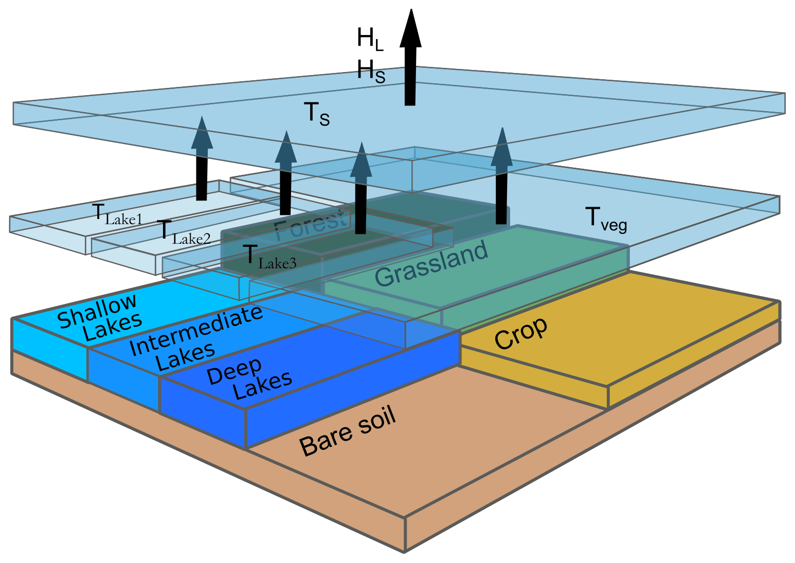
Figure 1 Multi-tile lake representation in the ORCHIDEE land surface model in a three-tile configuration.

3.2 FLake model refinements

3.2.1 Shape factor revision

As already noted, in FLake, the temperature profiles in the thermocline layer (but also in the sediment layer not activated in this work) are solved following the concept of self-similarity. The temperature profile in the thermocline is computed through a shape function parametrized by an empirical polynomial equation which satisfies boundary conditions at the top and at the bottom of the thermocline. The equation was proposed by Malkki and Tamsalu (1985) where two cases are differentiated depending on whether the mixed layer h is developing or retracting following Eq. (1).

$$\begin{array}{}\text{(1)}& {\mathrm{\Phi }}_{\mathrm{\Theta }}\left(\mathit{\zeta }\right)=\left\{\begin{array}{ll}\mathrm{1}-(\mathrm{1}-\mathit{\zeta }{)}^{\mathrm{3}}& \text{if }\mathrm{d}h/\mathrm{d}t>\mathrm{0}\\ \mathrm{1}-\mathrm{4}(\mathrm{1}-\mathit{\zeta }{)}^{\mathrm{3}}+\mathrm{3}(\mathrm{1}-\mathit{\zeta }{)}^{\mathrm{4}}& \text{if}\mathrm{d}h/\mathrm{d}t\le \mathrm{0}\end{array}\right.\end{array}$$

Φ_Θ represents the normalized temperature depending of the normalized depth ζ as follows:

$$\begin{array}{}\text{(2)}& \begin{array}{rl}{\mathrm{\Phi }}_{\mathrm{\Theta }}& ={\displaystyle \frac{T_{\mathrm{s}}-T\left(z\right)}{T_{\mathrm{s}}-T_{\mathrm{b}}}},\\ & \mathit{\zeta }={\displaystyle \frac{z}{D}},\end{array}\end{array}$$

where we define T_s as the lake surface water temperature, T_b as the lake bottom temperature and T(z) as the water temperature at the depth z.

Mironov (2008) defined a shape factor C_θ as the integration over the depth of the temperature profile. Equation (3) controls the evolution of the shape factor and allows the transition to be made between the two temperature profiles. This factor linearly changes with time and proportionally to a relaxing characteristic time t_rc between the two extreme values $C_{\mathit{\theta }}^{min}$ and $C_{\mathit{\theta }}^{max}$.

$$\begin{array}{}\text{(3)}& {\displaystyle \frac{\mathrm{d}{C}_{\mathit{\theta }}}{\mathrm{d}t}}=\mathrm{sign}(\mathrm{d}h/\mathrm{d}t){\displaystyle \frac{C_{\mathit{\theta }}^{max}-C_{\mathit{\theta }}^{min}}{t_{\mathrm{rc}}}},C_{\mathit{\theta }}^{min}\le C_{\mathit{\theta }}\le C_{\mathit{\theta }}^{max}\end{array}$$

Some issues were reported by Salgado and Le Moigne (2010) who found unrealistic behavior of the temperature profile in spring seasons for long-term simulations, with an overly large decrease in the bottom temperature. They reveal that the numerical instabilities of the shape factor during winter were playing a role in this issue. On our side, we observed similar instabilities even when no freezing conditions were encountered. Salgado and Le Moigne (2010) proposed to limit the shape factor time evolution to a threshold fixed to 0.01 h⁻¹ and to raise the minimum value $C_{\mathit{\theta }}^{min}$ from 0.5 to 0.65. They found that the deep temperature evolution with these changes was more realistic with a large decrease in the numerical instabilities. After some tests, we came to the same conclusions and chose to apply the same corrections to the shape factor parameterization.

3.2.2 Lake snow module

The snow module within FLake, which allows the simulation of the time evolution of the snowpack when the lake is frozen, was not well tested in its original parameterization (Mironov et al., 2010). The snow temperature is represented following the same approach as the one developed for the ice layer below, i.e., integral heat budget of the ice and snow layers and self-similarity assumption of the temperature profiles. At the snow–ice interface, Eq. (4) is used to calculate the snow temperature based on the condition of continuity of the heat flux.

$$\begin{array}{}\text{(4)}& T_{\mathrm{snow}}=T_{\mathrm{ice}}+R_{\mathrm{h}}\cdot (T_{\mathrm{ice}}-T_{\mathrm{freeze}})\end{array}$$

R_h is the ratio of the thermal resistance between the ice layer and the snow layer equal to $\frac{H_{\mathrm{S}}}{H_{\mathrm{I}}}\frac{{\mathrm{\Phi }}_{\mathrm{I}}^{\prime }\left(\mathrm{1}\right)}{{\mathrm{\Phi }}_{\mathrm{S}}^{\prime }\left(\mathrm{0}\right)}\frac{k_{\mathrm{I}}}{k_{\mathrm{S}}}$ where H_I and H_S are the ice and snow height and k_I and k_S are the thermal conductivity of ice and snow. This formulation can lead to numerical instabilities for high values of R_h. To fix this issue, Pietikäinen et al. (2018), when coupling the German REgional MOdel (REMO, Jacob and Podzun, 1997) with FLake, proposed to set a threshold for the ice layer thickness above which the snow layer can develop. On our side, we did not implement this solution and prefer to decrease the time step of the FLake snow module to prevent the numerical instabilities with the advantage of preserving the water budget. Several global test simulations were performed to adjust the time split factor. As a result, it appeared necessary to go down to time steps of the order of 1 min to remove all the instabilities. Therefore, it has been decided to set the time split factor to a value of 50 and to activate it only when the snow thickness is less than 3 cm. Other improvements to the snow module of FLake were proposed by Semmler et al. (2012). The improvements concern the parameterizations of the snow density, the thermal conductivity and the snow and ice albedos. Based on data acquired on Lake Bear in Canada, Semmler et al. (2012) revised the snow density relationship with height, which can lead to unrealistic values during the melting period, and tested various parameterizations including the use of a constant value of 320 kg m⁻³. Their results show the benefit of parameterizations accounting for snow aging, but given that the use of a constant value permitted them to better represent the snow and ice cover dynamics compared to the original FLake parameterization, we chose this option as a first step.

The original equation of the snow thermal conductivity $k_{s_{\mathrm{eff}}}$ was given by Eq. (5) with $k_{s_{\max }}$ and $k_{s_{\min }}$ the maximum and minimum values of the snow heat conductivity and h_s the snow depth. It was replaced by Eq. (6), where $k_{s_{\mathrm{eff}}}$ varies between the ice and snow conductivity values according to the snow layer thickness. The bounds of the interval were set to 0.14 W m⁻¹ K⁻¹ for the heat conductivity of the fresh snow k_s and 2.29 W m⁻¹ K⁻¹ for the heat conductivity of the lake ice k_i and the empirical constant c was fixed to a value of 5 m⁻¹, following Semmler et al. (2012).

$$\begin{array}{}\text{(5)}& {\displaystyle }{k}_{s_{\mathrm{eff}}}=min(k_{s_{\max }},k_{s_{\min }}+\mathrm{1.3}\cdot h_{\mathrm{s}}\cdot {\displaystyle \frac{{\mathit{\rho }}_{\mathrm{s}}}{{\mathit{\rho }}_{\mathrm{w}}}})\text{(6)}& {\displaystyle }{k}_{s_{\mathrm{eff}}}=k_{\mathrm{s}}+(k_{\mathrm{i}}-k_{\mathrm{s}})\cdot e^{c\cdot h_{\mathrm{s}}}\end{array}$$

Following Semmler et al. (2012), Pietikäinen et al. (2018) also revised the calibration of the ice and snow albedos and proposed to change the white (blue) ice albedos values from 0.6 (0.1) to 0.5 (0.3) and the dry (melt) snow albedo values from 0.6 (0.1) to 0.87 (0.77). We implemented the same modifications in our developments.

3.3 Model settings

ORCHIDEE requires the description of the land surface variability in each model grid cell to simulate the energy and biogeochemical processes. As already noted, the standard version uses PFT maps derived from the CCI Land Cover product. Since the standard PFT maps do not consider water surfaces, the permanent water bodies from the CCI Land Cover product have been merged with the bare surfaces in the corresponding PFT. The new splitting in SFTs with different energy budgets calculation requires that lake fraction is first removed from the bare soil fraction and transferred to the new lake SFT. For that purpose, new PFT maps excluding lakes for each year of the simulation have been generated. In a second step, we have worked on the definition of the lake fraction within a grid cell and the need to split it according to the depth, following the recommendations of Bernus et al. (2021). Indeed, one important outcome of our previous work was to quantify the role of FLake parameters in the simulation of the surface variables and to show that depth is especially determinant in the case of shallow lakes. Therefore, we decided to prescribe the number of lake tiles in our model. This new parameter, that has to be set prior to the simulation, allows the definition of different types of lakes within a grid cell, differing by their input parameters (depth, surface area, radiative properties, etc.). The methodology developed to define those parameters is presented in the following.

3.3.1 Lake surface area and depth

The HydroLAKES database (Messager et al., 2016) was analyzed to parameterize lake surface area and depth in ORCHIDEE. In the study of Bernus et al. (2021), three categories were defined according to depth ranges: shallow lakes with depth below 5 m, deep lakes with depth larger than 25 m and the intermediate class in between (depth range between 5 and 25 m).

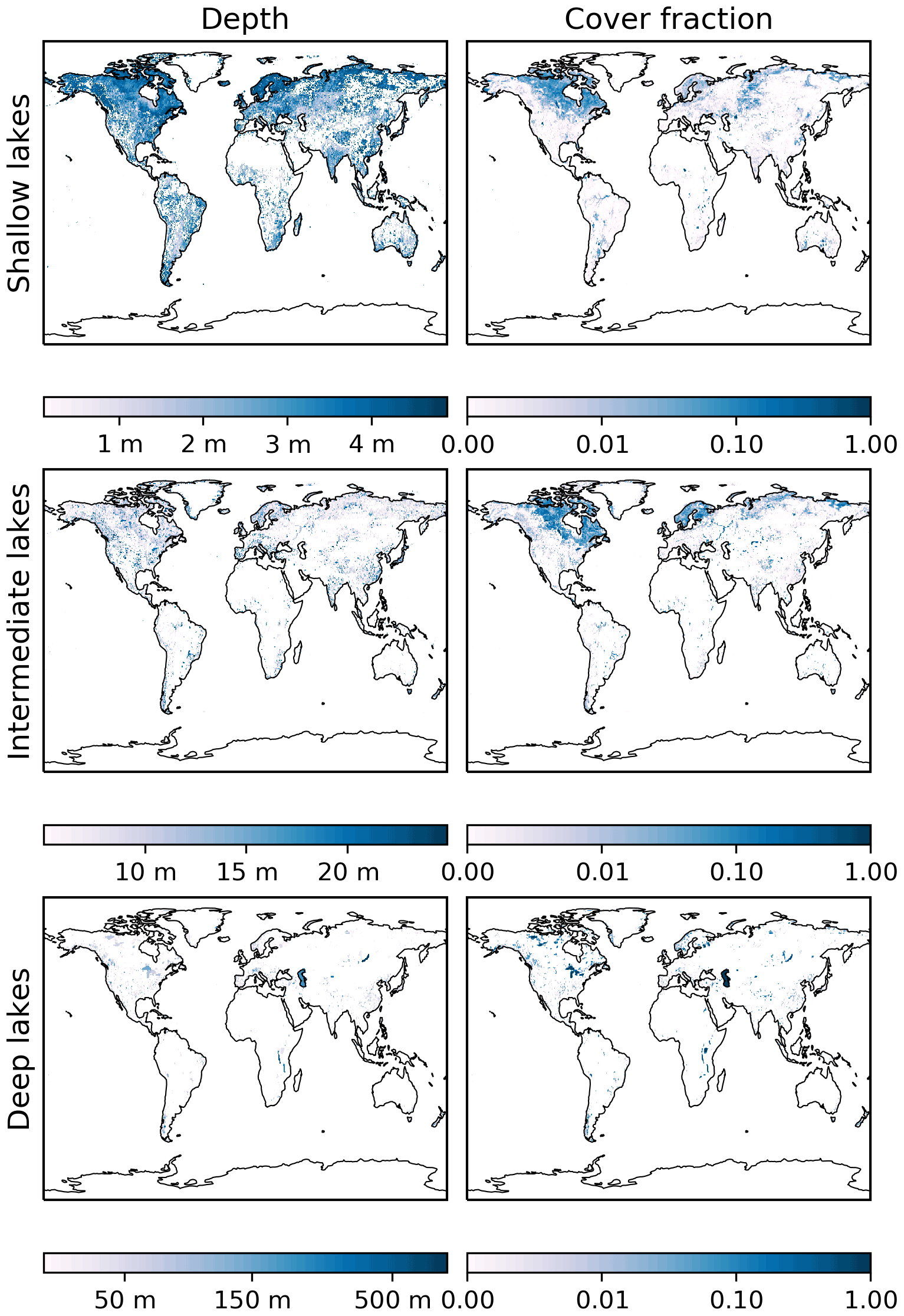
Figure 2 Lake depth (left column) averaged for each lake categories: shallow (below 5 m), intermediate (between 5 and 25 m) and deep (above 25 m), and cover fractions (right column) at a spatial resolution of 0.5^∘.

Figure 2 shows the lake surface fractions (in logarithmic scale), plotted at 0.5^∘ resolution, for the three categories of lake depths and aggregated in a single class. The median values of the corresponding depths are shown in the same figure. The higher amount of lake surfaces in the high northern latitudes, mainly in northern Canada, Scandinavia and western Siberia, are clearly highlighted. The lake distribution shows a minimum at the latitudes between 20^∘ N and −30^∘ S, in coherence with the arid climates found at these latitudes, produced by the descending branch of the Hadley circulation. The plots of the corresponding depths show a higher concentration of shallow and intermediate lakes in the northern high latitudes, whereas deep lakes look well distributed on all the continents. The major big lakes appear clearly on the plots, such as the Great Lakes in Canada, Lake Victoria in South Africa, Lake Malawi in South America, and Lake Baikal and the Caspian Sea in Eurasia. It can be noted that when ORCHIDEE is fully coupled to the IPSL ESM, the Caspian Sea is handled like the other seas and oceans in the ocean model NEMO (Madec et al., 2008).

3.3.2 Other lake parameters

FLake requires the prescription of other parameters like the radiative parameters of water (surface albedo and extinction coefficient) and the wind fetch. For the radiative parameters, the standard values and parameterizations proposed in FLake have been kept. Therefore, an albedo of 0.07 and an extinction coefficient of 1 m⁻¹ was set for water. The fetch parameter, which appeared less influential in the sensitivity analysis performed by Bernus et al. (2021), has been defined according to the mean of the fetch values estimated for all the lakes falling in the ORCHIDEE grid cell. More precisely, the fetch for a given lake was approached from its surface extent. Assuming a circular pattern, the fetch was set to the diameter of a circle of equivalent surface, and the effective fetch of the tile was derived from the aggregation of the fetch values of all the lakes falling in the lake tile considered (mean average).

3.4 Performed experiments

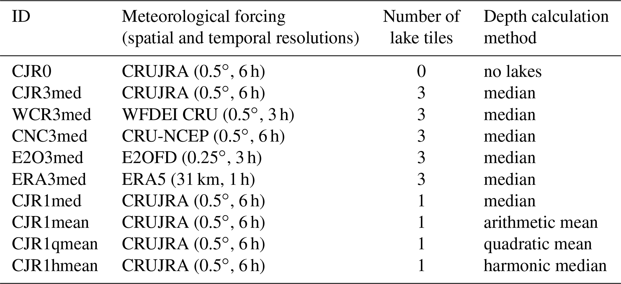
ORCHIDEE-FLake was run at global scale forced by the various atmospheric datasets presented in Sect. 2.1.5 and for two different configurations of lake tiling: the first one when all the lakes are grouped in a single class and the second one, where lakes are grouped in three classes according to lake depth. A control simulation corresponding to the standard ORCHIDEE configuration without lakes (i.e., considered as bare soils) and using only one atmospheric forcing (CRUJRA) was also performed. Table 1 presents the list of all the simulations performed, the atmospheric forcing used and its spatial resolution, the number of lake categories, and the way the depth was set for each class (median depth value of all the lakes within the tile, arithmetic, quadratic or harmonic averages). All the simulations were run on the period (1979–2016) at a time step of 30 min. The first 20 years (1979–1999) were used as spin-up to bring the prognostic variables to equilibrium. Therefore, the results were analyzed over the period 2000–2016. The name of each simulation is composed of three letters referring to the atmospheric forcing, one number corresponding to the number of lake tiles and between three and five characters referring to the way the depth has been averaged. Then, the comparison of CJR3med to CJR0 allows the assessment of the contribution of lakes on the ORCHIDEE surface variables. Comparison of CJR3med to CJR1med allows the impacts of the number of lake tiles and the way of averaging to be seen in the comparison of CJR1med to CJR1mean, CJR1qmean and CJR1hmean. Finally, the comparison of CJR3med to WCR3med, CNC3med, E2O3med and ERA3med allows the impact of the atmospheric forcing and the related uncertainties to be highlighted. The performance metrics, i.e., the RMSE, the MSE and its components, used in the evaluation are presented in the Appendix A.

We also compared the aggregation depth of each experience to the depth of the observed lake in HYDROLAKES. To assess the model errors in the comparison to the observations, a preliminary step was to link the lakes from HydroLAKES to the GloboLakes ones. We succeeded in linking 964 of the 979 lakes of GloboLakes. The 15 missing lakes which were not present in HydroLAKES have not been included in the evaluation procedure. When GloboLakes and HydroLAKES were in agreement over a single lake, the depth referenced in HydroLAKES was assigned as the observed depth. But when several water bodies in HydroLAKES corresponded to a single observed lake, we assigned the area-weighted mean depth to assess the depth of the observed lake.

Table 1 List of the 10 ORCHIDEE-FLake simulations performed at global scale, differing from the atmospheric forcing used and the number of lake tiles considered in the ORCHIDEE grid cell.

4 Results

4.1 Evaluation at global scale

4.1.1 LSWT

The simulated LSWT values obtained in CJR3med configuration have been compared to the observations provided by GloboLakes for the 979 lakes matching ORCHIDEE simulated lake tiles. We recall that CJR3med corresponds to the simulation performed with the meteorological forcing CRUJRA and prescribing three lake tiles differing by their depth (shallow, intermediate and deep lakes). The comparison was done with the lake tile corresponding to the depth category of the observed lake. The RMSE calculated on the 17-year period (2000–2016) are plotted in Fig. 3 along with latitudinal and zonal averages. Each dot corresponds to a lake of the GloboLakes dataset. Figure 3 shows that the observations are well distributed globally and sampled a large variety of climates and continents. Their density is well correlated with the lake area distribution plotted in Fig. 2. Therefore, the LSWT errors calculated with GloboLakes should be a good representation of the ORCHIDEE-FLake model error. Since GloboLakes does not provide LSWT for frozen lakes, LSWTs below 0 ^∘C are not used in the RMSE calculations. The results show that most of the RMSEs are ranging between 2 and 4 ^∘C. Higher errors can be seen for a few lakes with RMSE values up to 8 ^∘C. The latitudinal representation highlights a positive trend of the RMSE, when moving from the temperate to the boreal regions. In the tropics, some large RMSE peak values are observed, which are all the results of individual lakes presenting large errors which impact greatly the zonal average. Because of the low number of lakes at these latitudes, a lake badly simulated has a larger impact on the performance metrics than in the higher latitudes.

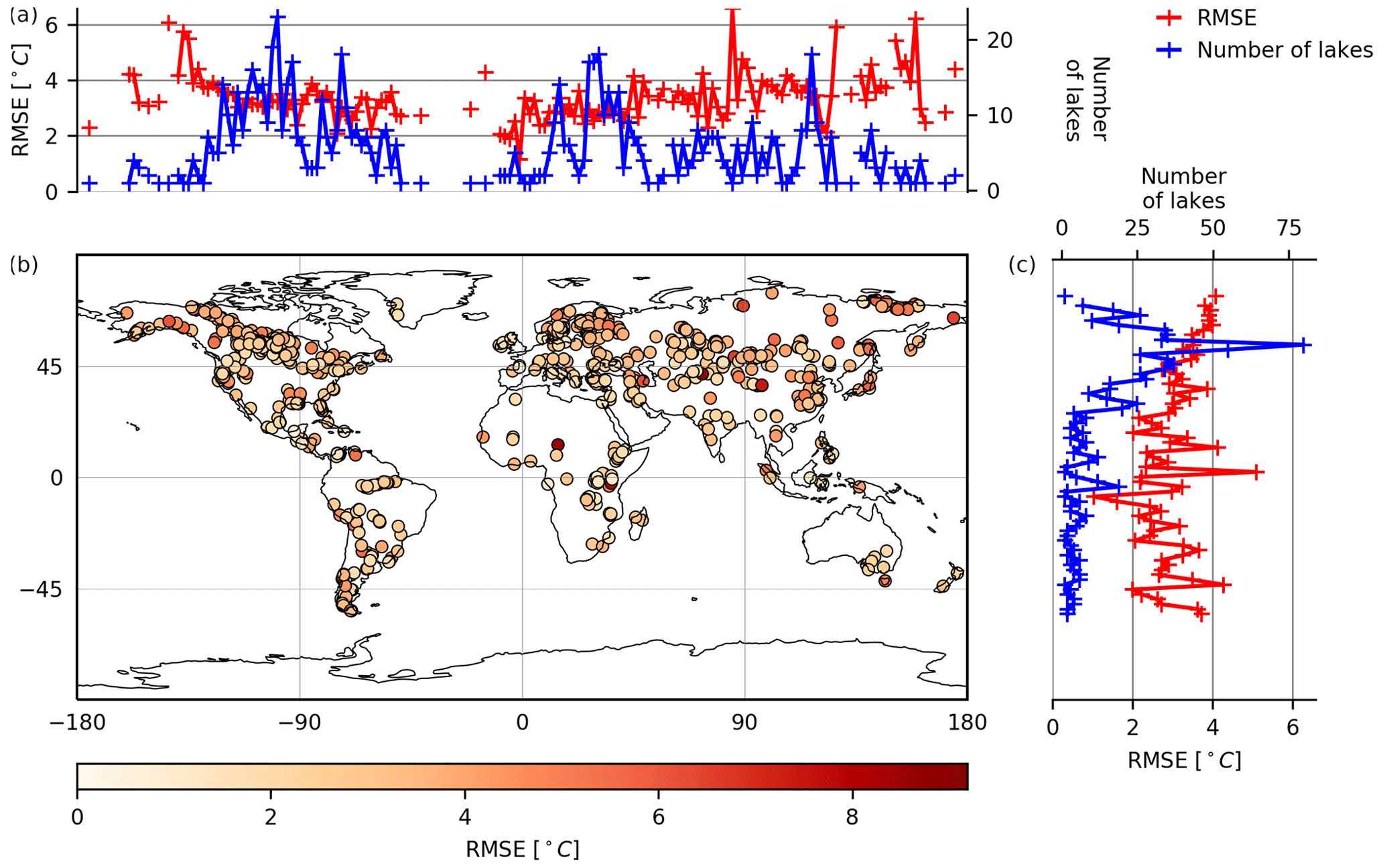
Figure 3 LSWT errors (RMSEs) simulated by ORCHIDEE-FLake in the CJR3med configuration run at 0.5^∘ resolution. Longitudinal (a) and latitudinal (c) averages of the RMSEs (in red) and number of lakes observed in GloboLakes (in blue) are plotted along the map.

4.1.2 Ice phenology

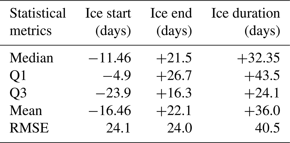
Freezing processes were evaluated against the data provided by the Global Lake and River Ice Phenology database over the lakes observed in the northern latitudes. Since the observations provide the dates of the full ice end, start and duration of a complete ice coverage, we compared with the same simulated dates and did not consider ice-free periods (if there were any) within this interval. In Table 2, the mean, quartiles and median of the differences between simulated and observed three stages of the ice phenology are given in days for the CJR3med simulation. The results show that the ice start errors are all negative and the ice end errors are all positive. That means that the lakes are generally freezing earlier and melting later in the model compared to the observations. Therefore, the simulated ice duration is larger. The mean bias on ice start is about −11 (median value), +21 d for ice end, leading to an ice duration overestimated by 32 d in average. The RMSE values are around 24 d for both ice start and ice end and reach 40 d for the ice duration error. The interquartile range is larger for ice start (19 d) compared to ice end (10 d) highlighting the fact that the ice start errors are more scattered. This also explains why the differences between the median and mean values are larger for ice start compared to ice end.

Table 2 Statistical metrics (simulations – observations) of the lake ice phenology (ice start, end and duration) obtained in the CJR3med configuration.

4.2 Sensitivity to meteorological forcing

4.2.1 Analysis on specific lakes

Model evaluation has been performed at the local scale for various lakes sampling a large variety of climates and lake properties, in particular their mean depth. Figure 4 presents the comparison of simulated LSWTs to observations for a selection of eight lakes. Among those, Victoria and Titicaca are located in tropical regions; Erie, Superior and Baikal in boreal ones; and Constance, Tahoe and Tai in more temperate ones. Lake Tai is a shallow lake, the others being deeper (mean depth of each lake is noted on the respective plots). Another criteria for the choice of these lakes was their spatial extent, covering at least one ORCHIDEE grid cell at 0.5^∘ resolution, enabling a better comparison with the observations. The LSWT time series (simulated and observed over the year 2010 chosen as an example) are plotted in Fig. 4 along with the MSE errors decomposed into its three components (Kobayashi and Salam, 2000), i.e., squared bias (SB), squared difference between standard deviations (SDSD) and lack of correlation weighted by the standard deviation (LCS), all represented in bar plots. We recall that the metrics are calculated only for positive values of LSWT, since GloboLakes observations do not consider frozen conditions.

Figure 4 shows that the seasonal variations of LSWT are generally well represented for all the lakes. The MSE values are ranging between 0.9 and 27.7 ^∘C² (i.e., RMSE between 0.95 and 5.3 ^∘C) but can show large variations according to the atmospheric forcing. The MSE decomposition shows that the model errors are either explained by biases or by deficiencies to simulate the fluctuation patterns, and less by failure to model the amplitude of the seasonal cycle, since SDSD is always much lower than the SB and LCS components. Among all the lakes, lakes Tai and Tahoe present the lowest errors and Lake Titicaca the largest ones for at least three of the forcings used. It is interesting to note that the results do not vary much among the forcings for a same lake, except for the two tropical lakes, Victoria and Titicaca, the latter showing the largest variability. Indeed, RMSE of Lake Titicaca is equal to 0.9 ^∘C when CRUJRA forcing is used and can be up to 5 ^∘C for CRU-NCEP or WFDEI-CRU forcings. It is the same for Lake Victoria where RMSE is around 0.95 ^∘C in the E2OFD simulation and up to 3.5 ^∘C in the WFDEI-CRU one, all these errors being explained mainly by biases.

For the other lakes, the errors are more homogeneous among the forcings, even if significant differences appear. If we consider the three temperate lakes, we can see that the annual surface temperature amplitude is larger than for the tropical ones, between 15 and 20 ^∘C. Lake Tai is well represented with MSEs below 8 ^∘C² (i.e, RMSE below 2.8 ^∘C) for all the forcings. For the two other temperate lakes (Tahoe and Constance), the model fails to simulate the annual amplitude which is slightly underestimated, and the cooling at the end of summer is delayed whatever the forcing used. For the Lake Constance, the SDSD component can reach 4.5 ^∘C². Such errors could result from parameterization errors, such as depth errors which are known to influence greatly the seasonal LSWT pattern.

The results obtained for the boreal lakes do not show the same features: the cooling after summer is generally well reproduced whatever the forcing used but the warming in spring looks too rapid for Lake Erie and Lake Superior and too late for Lake Baikal. Frozen processes show also large deficiencies in all simulations, with lakes Superior and Erie freezing in winter, contrary to the observations and an overestimation of the frozen season for Lake Baikal which is freezing by about 1 month in advance with CRU-NCEP forcing and melting one month too late, preventing to simulate correctly the temperature time evolution in spring. In these two cases, the simulations performed with E2OFD forcing show the best results in terms of MSE. The fact that the duration of the freezing period is largely overestimated whatever the atmospheric forcing could be the result of parameterization errors of the cryospheric processes that will be investigated in the following.

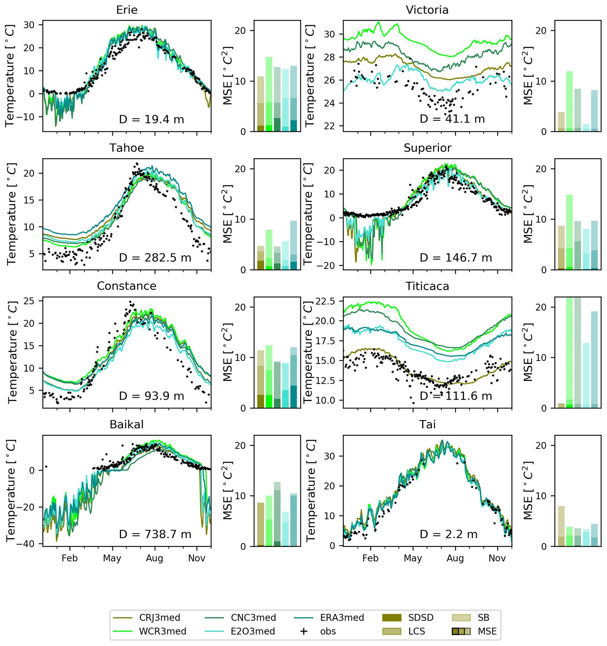
Figure 4 Example of time series of the daily mean lake surface temperature simulated for eight lakes with five different meteorological forcings compared to GloboLakes observations for the year 2010. The bar plots represent the decomposition of the MSEs in terms of bias (SB), lack of correlation (LCS) and difference of standard deviations (SDSD) (represented with different shadings) between the model and the observations.

4.2.2 Global-scale analysis

Figure 5 presents the performance metrics calculated on all the lakes observed in GloboLakes (i.e., 979 lakes all around the world). The comparison is done at the lake level with the corresponding ORCHIDEE lake tile the lake falls in (given its mean depth). The statistics were calculated for the 17 years of the whole simulation period (2000–2016). The metrics shown here are the RMSE, the unbiased RMSE and the three normalized components of the MSE, i.e., SB (with the sign), SDSD and LCS, in terms of fractions, calculated for each simulation forced by the five atmospheric forcings used. We recall that the sum of the three components is equal to unity.

The results show that the simulations forced by the meteorological reanalysis with the lower resolution (i.e., 0.5^∘) lead to the worst performances (higher RMSEs between 3.18 for CRUJRA, 3.16 for CRUNCEP and 2.82 ^∘C for WFDEI-CRU). When higher resolution forcings are used (E2OFD and ERA5), the RMSEs decrease to 2.81 and 2.69 ^∘C. An important part of the errors is therefore explained by the resolution and accuracy of the meteorological forcings. It should also be noted that ERA5 is based on the ECMWF atmospheric model which includes the HTESSEL land surface model accounting for lakes, unlike the other atmospheric products. This feature could lead to atmospheric surface variables of better quality over lakes and explain that the simulated lake surface temperatures are closer to the observations.

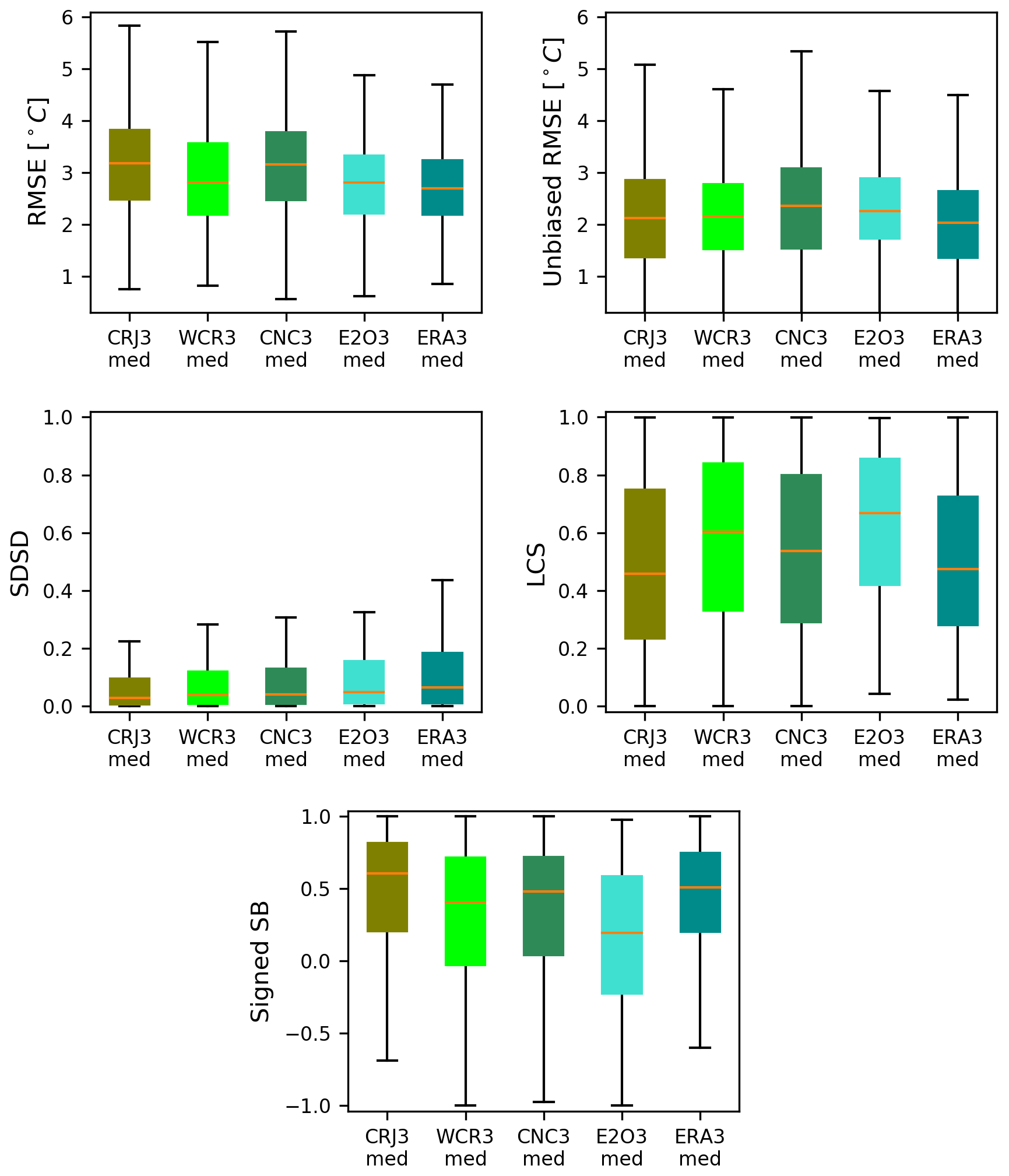
Figure 5 LSWT errors obtained on the 979 lakes observed in GloboLakes for the five simulations CRJRA3med, WCR3med, CNC3med, E2O3med and ERA3med. RMSE, unbiased RMSE, LCS, SDSD and sign SB are represented in boxplots. Median values are represented by orange lines, and quartiles by the edges of the color box.

However, the decomposition of the MSE is quite similar among the forcings on average. For half of the lakes, LCS component represents at least 45 % of the MSE error for CRUJRA and ERA5 simulations and up to 65 % for the E2OFD simulation. The SDSD component is very minor since it is less than 20 % of the MSE for more than 75 % of the observed lakes. Thus, the LSWT errors are firstly explained by the model biases and deficiencies to reproduce the seasonal patterns, confirming what was already noted for the individual lakes analyzed previously. In Fig. 5, we can see that the biases are positive for all the forcings, meaning that the model generally overestimates the surface temperature. The signed SB (median values) obtained with E2O 3med is the closest to 0. Compared to the total RMSE that can reach up to 10 ^∘C, the unbiased RMSEs are reduced and do not exceed 6 ^∘C.

The sensitivity of the simulated ice phenology to the meteorological forcing has been evaluated and the results are plotted in Fig. 6. The whisker plots show that the impact of the meteorological forcing is lower on the prediction of the start of lake freezing (ice start) than on the prediction of the end of the freezing period (ice end), and consequently on the ice duration where the two errors cumulate. It can be seen also that the errors are smaller for the two simulations performed with the higher resolution forcings (E2OFD and ERA5) with a significant advantage of E2OFD especially for the simulation of ice end. The ice start, ice end and duration median errors are respectively equal to −6, 11 and 20 d with E2OFD, whereas they are up to −14, 25 and 41 d with the CRUNCEP forcing.

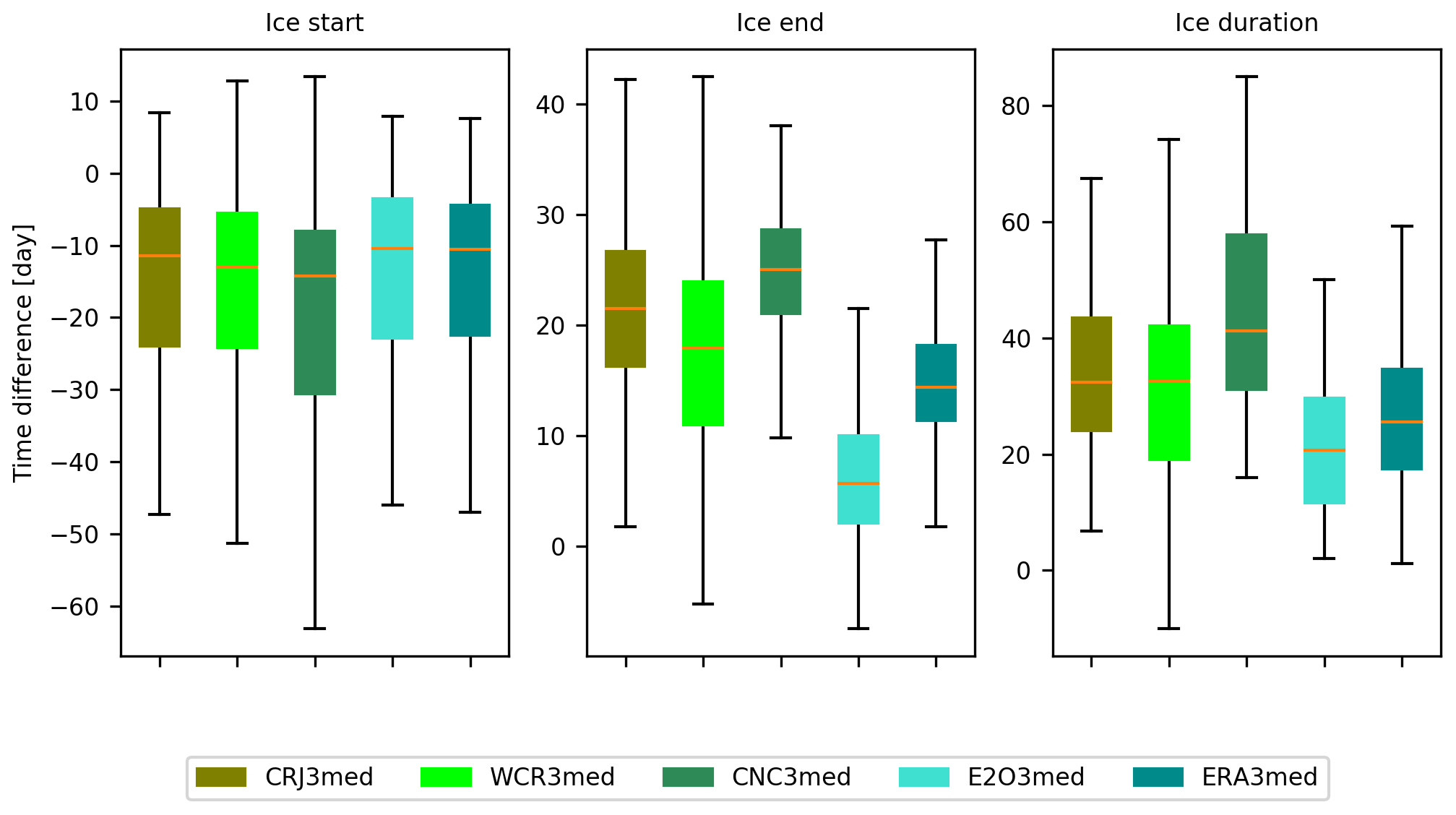
Figure 6 Boxplot of the model errors on the start, end and duration of the ice period for the five simulations CJR3med, WCR3med, CNC3med, E2O3med and ERA3med. Median values are represented by orange lines, and quartiles by the edges of the color box.

4.3 Sensitivity to lake depth parameterization

To understand the impact of the depth parametrization, we analyze the differences between the real depth of the 979 observed lakes and the depth prescribed in the corresponding ORCHIDEE tile at a grid resolution of 0.5^∘.

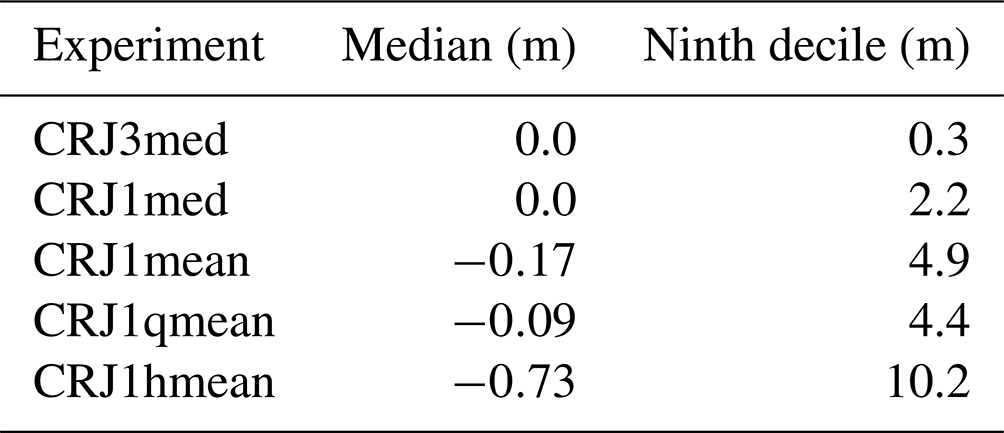
Figure 7 presents the distribution of the errors between the depth of the observed lake and the depth prescribed in the corresponding ORCHIDEE tile, for the five model configurations, i.e., median depth value calculated in a three-lake tile configuration (3med) and in the one-lake tile configurations (1med, 1mean, 1hmean and 1qmean). The histogram of the errors and the cumulative distribution functions (CDFs) are both plotted. Table 3 gives the median and the ninth decile of the depth error distribution.

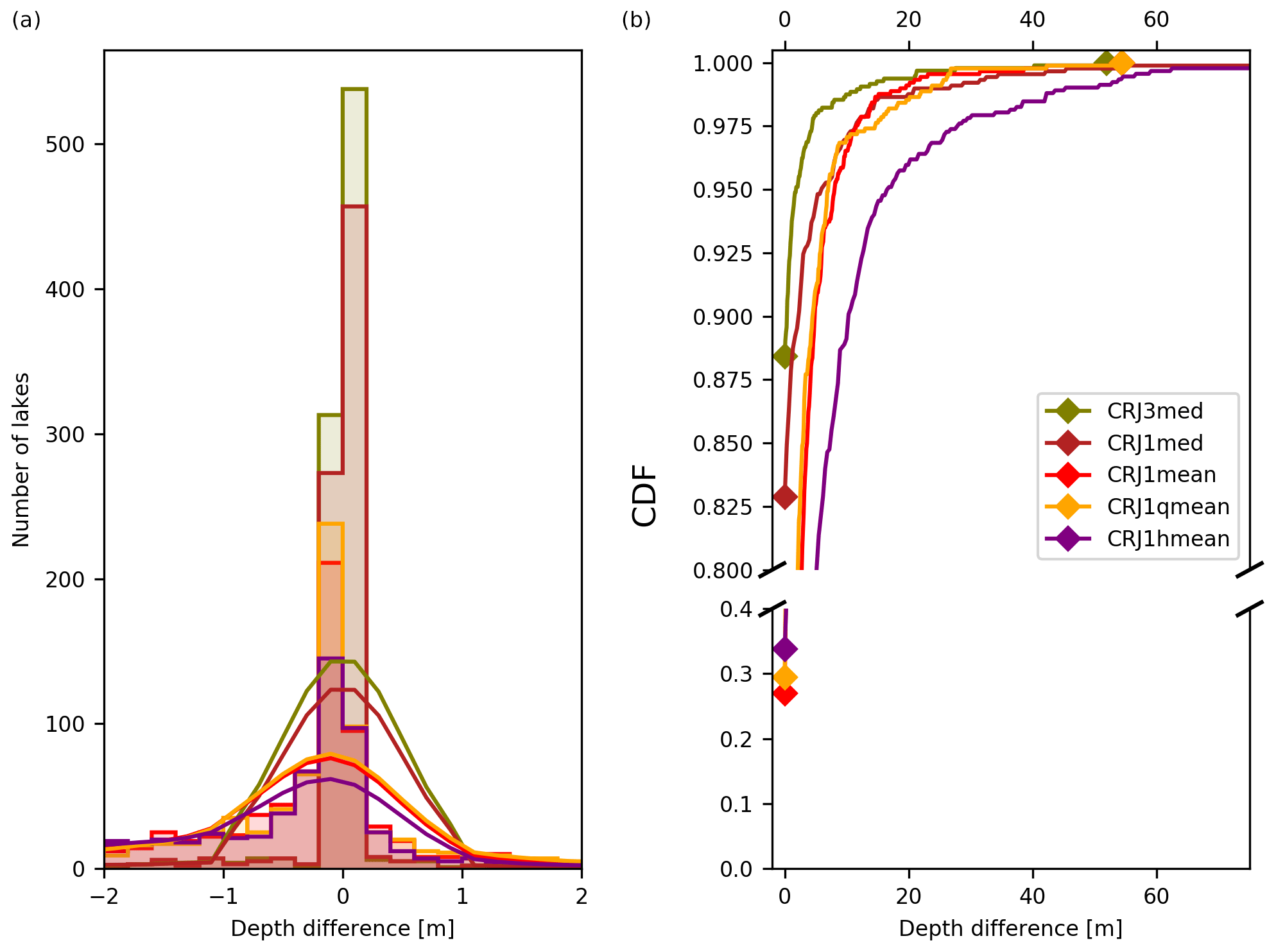
Figure 7 The histogram (a) and cumulative density function (b) of the depth errors between the observed and simulated lake for each depth parameterization strategy. In (a), the lines correspond to the smoothing of the histogram with a Gaussian window.

The histogram of the errors are well centered around 0 for the three-tile configuration and the one-tile one when the median average is performed. The three other ways to aggregate the lake depths (arithmetic, quadratic and harmonic means) show negative biases (the median ranging between −0.1 and −0.7 m) illustrating the fact that grouping all the lakes of the same mesh in a single tile leads to a slight underestimation of the representative depth. This is probably the result of the worldwide lake distribution previously presented in Fig. 2, showing that shallow lakes are more numerous and cover a larger extent than deeper lakes. This is confirmed by the CDF curves plotted in Fig. 7 showing that the configuration with three tiles presents the lowest errors on the depth parameterization, and the median appears to be the best way of depth aggregation in the one-tile configurations. Indeed, we have seen that about 90 % of the observed lakes have an absolute error less than 0.3 m in the three-tile configuration and less than 2.2 m when the depth parameter is set to the median value within the lake tile. In comparison, 90 % of the observed lakes have an absolute error less than 4.4 m with the quadratic mean and less than 4.9 m with mean depth estimation approach. The harmonic mean is the worst approach since 10 % of the observed lakes have an absolute depth error larger than 10.2 m.

Table 3 Statistical metrics of the depth error distributions according to the depth parameterization strategy used: the median and ninth decile values are given in meters.

In Fig. 8, the LSWT errors obtained for all the simulations using the one-tile configuration are compared to the three-tile simulation already presented in Sect. 3.4. The total and unbiased RMSEs, SDSD and LCS and the signed bias are plotted as box plots. Compared to the previous sensitivity analysis to the atmospheric forcing, the errors are slightly lower, as is the dispersion among the simulations. The RMSE values are generally lower than 6 ^∘C with a median value between 3.1 and 3.2 ^∘C. The components present a similar order of magnitude among the simulations with positive bias and lack of correlation (LCS) explaining most of the MSE, as already seen in the three-tile configuration. This result was expected since the lake depth parameter in FLake mostly impacts the pattern of the seasonal cycle of LSWT and to a lesser extent its amplitude.

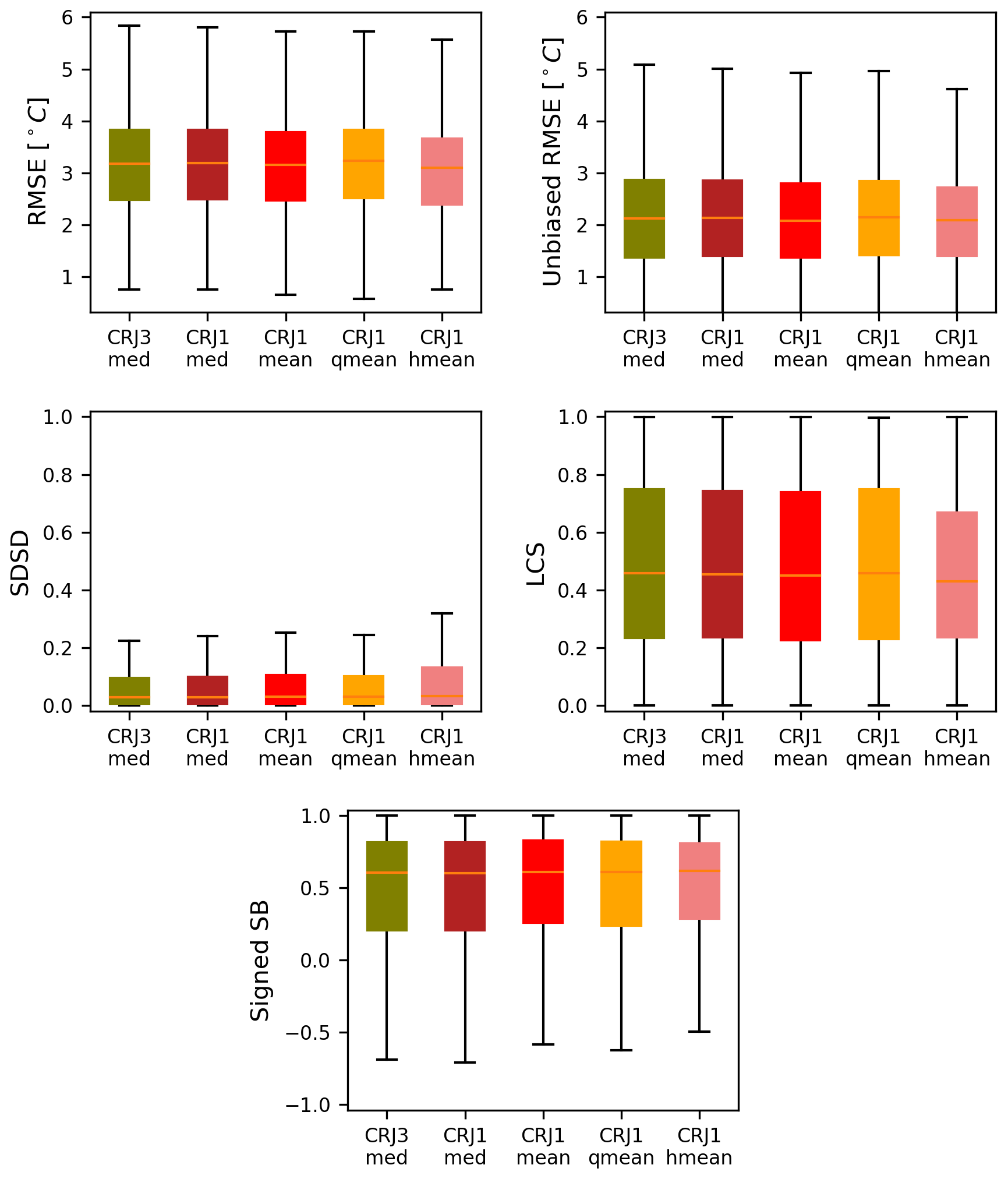
Figure 8 LSWT errors obtained on the 979 lakes observed in GloboLakes for the five simulations CJR3med, CJR1med, CJR1mean, CJR1qmean and CJR1hmean. RMSE, unbiased RMSE, LCS, SDSD and SB are represented as boxplots. Median values are represented by orange lines, and quartiles by the edges of the color box.

The ice phenology sensitivity to the number of lake tiles and depth parameterization strategy is presented in Fig. 9. Here also, the results show less impact compared to the sensitivity obtained with the meteorological forcing. In contrast, it appears that the ice start errors are reduced by half in the one-tile configurations compared to the three-tile one. In the four one-tile simulations, ice start errors are around 5 d, whereas it is equal to 10 d in the CJR3med simulation. However, the variance is quite similar, and the three-tile simulation shows a clear bias not observed in the one-tile simulations. Ice end and duration errors are similar among the five simulations, equal to about 22 and 27 d respectively, comparable to what is obtained in the CJR3med simulation. The improvement observed in the simulation of ice start in the one-tile simulations compared to the three-tile one, despite the increased depth errors, can be explained by the model biases. As a matter of fact, we highlighted in Sect. 4.2.1 the systematic underestimation of ice start time: LSWT cooling at the end of summer is too rapid and the lake freezing is earlier compared to the observations. If we consider that the shallow lakes represent a larger fraction of the lakes which are most likely to freeze and that the depth parameter of this class is the most impacted in the one-tile configuration, it is clear that parameter errors are compensating model deficiencies. The depth of shallow lakes, is most likely to be overestimated in the one-tile configuration. The deeper the lake, the later the start of freezing. Therefore, the depth overestimation will help to compensate the overly early cooling. The impact of this error is less visible on the ice end because the depth parameter is less influential during the ice melting process (Bernus et al., 2021).

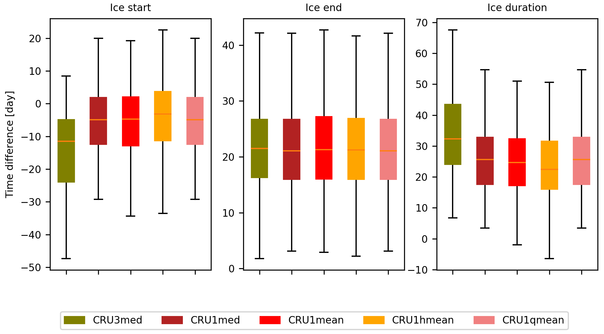
Figure 9 Boxplot of the RMSE errors on the start, end and duration of the ice period for the five simulations CJR3med, CJR1med, CJR1mean, CJR1qmean and CJR1hmean. Median values are represented by orange lines, and quartiles by the edges of the color box.

4.4 Energy balance impacts of lakes in ORCHIDEE

To analyze the impact of representing lakes on the global energy and water budgets, the two simulations CJR0 et CJR3med were compared at the global scale. The differences (CJR3med-CJR0) in terms of surface temperature, latent and heat fluxes averaged over the grid cell, were calculated for the four seasons of the year and plotted in Fig. 10. Winter period is defined as the average of the December, January and February months, summer as the average of June, July and August.

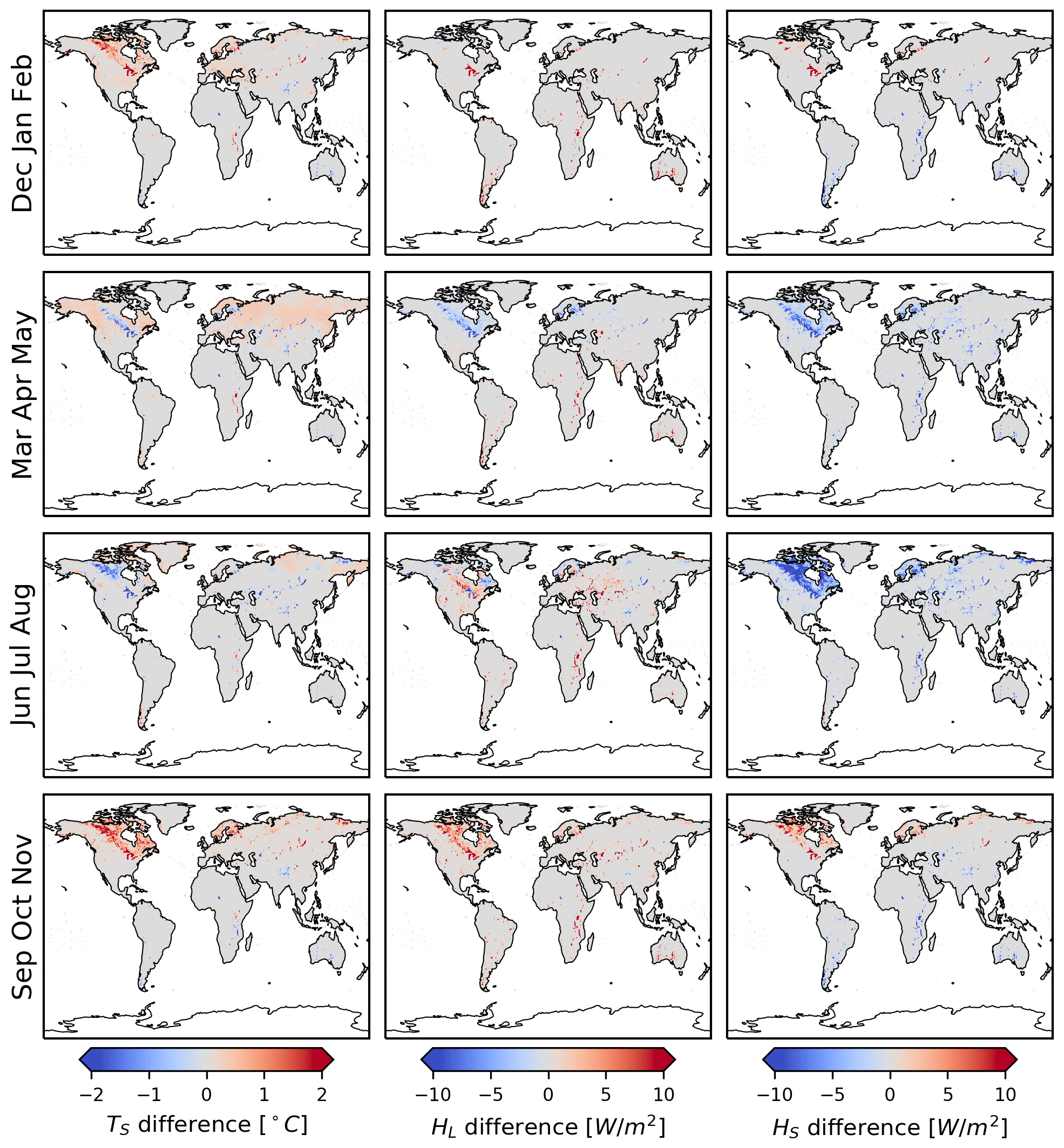
Figure 10 Differences (CJR3med − CJR0) in the surface temperature (first line) latent heat flux (second line) and sensible heat flux, simulated with and without lakes, averaged over 3-month periods starting from December (one per column).

The comparison of the two simulations (with and without lakes) shows interesting features. First, the surface temperatures appear warmer during a large part of the year, except for summer where the regions presenting large fractions of lakes of intermediate depth appear colder. In the high latitudes during the winter and autumn seasons, the temperature is generally warmer for all kind of lakes. For the deeper lakes, this difference can reach 10 ^∘C. It is the case for Lake Baikal, whereas for the Michigan and Superior lakes the difference is between 5 and 7 ^∘C. In the regions covered by smaller and shallower lakes in Scandinavia and Canada, this difference remains below 2 ^∘C due to the lower lake fraction and smaller smoothing effect of shallower lakes. In spring, the deep lakes as the great American lakes or Lake Baikal are cooler than their environment and explain the differences of temperature between the two simulations by 5–6 and 3–4 ^∘C respectively. However, the regions where the lakes are shallower remain warmer in the lake simulation because of their lower thermal inertia (but only by 0.5 ^∘C). In summer, most of the lakes are cooler in the northern latitudes compared to a neighboring bare soil, and the differences between the two simulations are always positive. In tropical latitudes, the pattern is different. During the humid season between October and April, the simulation with lakes is warmer at the end of the humid season by 1 or 2 ^∘C (in Africa during the spring season) and cooler during the end of the dry season by 0 or 3 ^∘C (in Africa).

Averaged at yearly timescale, the simulated global evaporation is 1.07 with lakes and 0.82 mm d⁻¹ without lakes. Focusing on the summer period, the global evaporation rises up to 1.72 with lakes and to 1.50 mm d⁻¹ without lakes when lakes occupy at least 20 % of the cell fraction. Then, the contribution of lakes raises the summer evaporation by 0.22 mm d⁻¹. For a grid cell completely covered by water, i.e., lake fraction equal to 1, the evaporation difference can reach 0.31 mm d⁻¹. In tropical areas, during the summer period and for latitudes below 30^∘ N, this difference is larger and equal to 1.16 mm d⁻¹ when the lake fraction is above 20 % and amount to 1.6 mm d⁻¹ when the lake fraction is equal to 1.

In terms of fluxes, the latent heat flux is generally stronger everywhere during part of spring and summer as is shown by the rise of the mean evaporation rates. In spring and in the northern latitudes, the latent heat flux is lower in the simulation with lakes, because of the freezing processes which prevent the lake evaporation. Compared to a bare soil that starts to evaporate earlier in ORCHIDEE, the lake evaporation is lower in early spring. For example, the latent heat flux of Lake Baikal is between 25 and 50 W m⁻² less than the bare soil evaporation and it is about the same for Lake Superior (between 20 and 40 W m⁻²). The freezing duration is longer for a lake than for a bare soil. The sensible heat fluxes are generally weaker everywhere during part of spring and summer because of the larger latent heat fluxes in the simulation with lakes.

5 Discussion and conclusion

This work presents how lake energy balance is now represented in the ORCHIDEE land surface model, thanks to the FLake lake model. The methodology and the model evaluation at global scale were presented. Several simulations were performed to evaluate the model sensitivity to the meteorological forcing and to the depth parameterization of the lake tile. The evaluation of LSWT and ice phenology against the GloboLakes and Global Lake and River Ice Phenology databases showed that the lake surface temperature is quite well simulated in this new ORCHIDEE version. Compared to the observations, LSWT errors range between 2 and 4 ^∘C, even if in some few cases, the errors can reach 8 ^∘C. These results are comparable to what was obtained by previous works, such as that of Dutra et al. (2010), who obtained RMSEs around 3.75 ^∘C in the high latitudes (>40^∘) and around 2.25 ^∘C for low latitudes (<40^∘) as median values. The lake ice phenology evaluation showed that the ice–snow coupled processes are also fairly well simulated with ice duration errors explained partly by start of freezing errors. Here also, compared to previous studies, the results obtained are quite similar. As an example, Dutra et al. (2010) obtained an ice start error of 30 d (in advance) for 75 % of lakes after optimization of the depth parameter against LSWT observations. The expected impacts of lakes on the near-surface atmospheric variables have been assessed by comparing the grid-cell-averaged surface temperatures and fluxes simulated by ORCHIDEE, considering lakes energy balance or not (in that case, lakes were considered as bare soils). The results show larger evaporation rates at the annual scale (around 0.25 mm d⁻¹) and smoother LSWT seasonal amplitudes. The impacts of these added fluxes on the atmosphere should be significant at regional scales, in particular on precipitation-predicted fields. As an example, Van de Walle et al. (2020) showed that Victoria lake evaporation explains up to 50 % local precipitation and storm events. The addition of lakes in the IPSL climate model is expected to produce similar impacts, helping to better reproduce the near-surface variables, the precipitation regimes and the extreme events.

5.1 Atmospheric forcing uncertainties

A large part of the LSWT errors is explained by the atmospheric forcing uncertainties. We have examined in more detail the lakes which present the largest RMSEs. Among the 969 lakes studied, only 15 present large RMSEs, larger than 6 ^∘C. For those lakes, we observed strong biases in the atmospheric temperatures and downwelling longwave radiation (whatever the reanalysis product), which explain the largest part of the error. If we consider the whole dataset, our results show the large sensitivity of LSWT to the atmospheric conditions and the large uncertainties of the reanalysis products. When looking to the RMSE decomposition, biases were explaining more than 50 % of the error for more than 50 % of lakes. It was particularly the case for the tropical lakes where the LSWT seasonal amplitude is lower than for higher-latitude conditions. The model sensitivity to the atmospheric conditions is also very strong during the intermediate seasons for the lakes which are subject to freezing. Because of the non-linearity of these processes, a small bias in the air temperature can completely change the temperature evolution of the lake and greatly influence the seasonal pattern and the ice phenology. The large sensitivity of the ice start and ice end times to the atmospheric forcing shown in our simulations is a good demonstration of this effect. Therefore, it appears very necessary to use various atmospheric forcing products in the model evaluation, since they all contain biases, which on top of that, present regional features. These biases are the result of the different atmospheric models and datasets used in the generation process, which consists of merging model simulations and multiscale observations through data assimilation techniques. It should be noted that the land surface models used in this process do not account for lakes except for the ERA5 forcing and are constrained by static land cover maps which are not updated regularly. Biases are also linked to the spatial and time resolution of the datasets. It has been shown that LSWT errors were smaller when the two high-resolution forcings are used (E2OFD and ERA5). Increasing the spatial resolution improved LSWT RMSEs by 0.5 ^∘C. Grid resolution is indeed an important parameter for the modeling of land surfaces which have very different functioning than the rest of the environment. Moreover, the atmospheric conditions above a lake surface are different than in the surroundings, complicating greatly the model evaluation at global scale. The use of various reanalysis products is, therefore, the only way to separate forcing and model errors.

5.2 Model parameterization

Systematic model errors appeared among the simulations and could be the result of parameterization errors. Sensitivity to depth parameterization was highlighted in previous works. Our simulations did not show a large impact of the depth parameterization at global scale on the LSWT error statistics, but the impacts on the ice phenology were shown to be significant, especially in the determination of the time of the start of freezing (ice start). As already said, the influence of lake depth on lake freezing is stronger than on ice melting, which is more driven by the atmospheric conditions and the amount of snow than the lake features directly. These results are in line with those obtained by Choulga et al. (2019), who previously showed the impact of the lake depth on the ice phenology.

Scaling issues may explain also part of the errors: FLake is a 1-D model and therefore does not consider the spatial variability of the within lake thermal processes and properties, nor the temporal variability of the parameters. In particular, the lake depth is a constant parameter in FLake, whereas it is clear that in reality, it varies spatially and temporally, and so do LSWT and ice phenology. Lakes, especially those subject to anthropogenic management as reservoirs, see their surface and water level changing throughout the year. The averaged depth and surface area referenced in the databases do not report these changes. For example, Lake Chad in HydroLAKES has a surface area doubled compared to the current value, and the average depth is probably erroneous as well. As well as this, if we consider the ice observations, the time of ice start refers to a complete ice coverage, whereas it can take some days before the lake is completely frozen. In contrast in FLake, because of the 1-D assumption, the lake surface is considered completely frozen when the surface temperature falls below 0 ^∘C. Then, the ice layer starts to grow and so will abruptly vary the related radiative parameters. For big lakes with large surface areas, this scaling error may be important. Similar conclusions were drawn by Pietikäinen et al. (2018), who identified two factors explaining the delay in their simulated ice end and the advance of ice start with the coupled FLake-REMO model. Because lakes are freezing too early, the snow accumulation can start earlier. An overestimation of the snow cover may explain the delay in the timing of the end of freezing and the overestimation of the ice duration period. To overcome this issue, the parameterization of the freezing processes could be revised by accounting for a partial ice cover as proposed by Choulga et al. (2019) or Garnaud et al. (2022), for example. In these two studies, the ice coverage is defined according to the ice layer thickness and so are the radiative properties. Such a modeling could help to slow down the freezing processes in FLake and improve the modeling of the surface temperature and fluxes. The prescription of a constant average value of the snow conductivity in our simulations could also play a role in the deficient representation of the dynamics of the ice and snow melting. Moreover, processes such as the snow erosion and transport by the wind are not modeled and may lead to an overestimation of the snow accumulation in the simulations.

Scaling and parameterization issues may affect other parameters like the radiative ones: albedo and extinction coefficient were both prescribed as constant values in space and time. This assumption may also impact the model performances. Recent databases can be used to solve this issue, based on satellite measurements. Albedo products could be used to spatialize the albedo parameters. The extinction coefficients are also known to be key (Heiskanen et al., 2015). For example, Zolfaghari et al. (2017) demonstrated the improvements brought by constraining the extinction coefficient of Lake Superior using FLake, based on remote sensing observations.

Missing processes could also explain part of the errors such as the impact of water salinity, which could present seasonal and interannual variations linked to human activities and water level changes. In our evaluation, among the 15 lakes presenting the largest errors, three of them are saline lakes (Issyk-Kul, Urmia and Natron) with high salinity levels, and which can present salt crust regularly (Zavialov et al., 2018, Sima et al., 2013, Tebbs et al., 2013). Salinity impacts surface albedo and evaporation (which is lower compared to those of freshwater), and consequently the surface temperature and its seasonal evolution. As reported by Ahmadzadeh Kokya et al. (2011), the temperature rising during the summer can be more rapid for saline lakes, as they observed for the Urmia lake in Azerbaijan. The consideration of salinity could therefore improve the modeling of the energy balance in the regions subject to high evaporation and also the modeling of the cryospheric processes in the cold ones.

5.3 Future work

Our results have shown the potential of ORCHIDEE-FLake coupled model to represent the energy balance of lakes, the surface temperature and fluxes at the atmosphere interface. The model performances are satisfactory, and the various sources of errors are well identified. The flexibility of our developments allows a variable number of lake tiles within a model grid cell to be prescribed and opens new perspectives for improvement. First, we intend to study the spatial and temporal variability of the lake radiative parameters and to implement them in the model. Data from high spatial resolution optical sensors such as Sentinel-2 with a 10 m resolution are very promising, and some products have recently came out such as that shown in Wang et al. (2020) for the lakes of the Tibetan plateau, or Zolfaghari et al. (2017) for the Erie Lake.

Lake area and depth are key parameters of the model. Thanks to satellite altimetry, water level changes as well as surface areas can be monitored. Future instruments such as the next SWOT mission will soon provide these data at the global scale for lakes larger than 250 m × 250 m with a temporal resolution varying along the swath but better than 21 d (Biancamaria et al., 2016). Such data will be of tremendous interest to improve the calibration of both lake depth and area in FLake. As well as this, the data will be also key to constrain water volumes, since resolving the lakes mass budget is the next development planned in our model.

Our preliminary results have shown that lakes are expected to impact the near-surface atmospheric fields. These impacts have already been shown by numerous studies such as the one of Le Moigne et al. (2016). The coupling of ORCHIDEE-FLake to the atmospheric model LMDZ is another mid-term perspective that will require developments in LMDZ to account for different atmospheric columns within an ORCHIDEE grid cell. But before that, simulating the thermal processes in lakes provides the possibility to model other biogeochemical cycles, in particular fluxes of GHGs like carbon dioxide and methane. Then, the tools developed are opening the path to studies on the contribution of lakes to global warming and impacts of climate and environmental changes.

Appendix A: Performance metrics

Bennett et al. (2013) describes several methods to characterize model performances. A simple way is to use an index such as the root mean square error (RMSE) which is widely used to measure the performance of a model and is defined by Eq. (A1).

$$\begin{array}{}\text{(A1)}& \mathrm{RMSE}=\sqrt{{\displaystyle \frac{\mathrm{1}}{N}}\mathrm{\Sigma }(T_{\mathrm{sim}}-T_{\mathrm{obs}}{)}^{\mathrm{2}}}\end{array}$$

To better understand the errors, we decomposed the MSE (the square of the RMSE) into three components: the squared bias (SB), the lack of correlation weighted by the standard deviation (LCS) and the squared difference between standard deviations (SDSD). After normalization, the sum of these three components is equal to unity. The demonstration of this decomposition is done with the method described by Kobayashi and Salam (2000). LCS evaluates if the model correctly reproduces the temporal pattern and SDSD if the model gives the correct temporal amplitude. We also used the signed squared bias (SSB) to analyze the sign of the biases and identify systematic errors.

$$\begin{array}{}\text{(A2)}& \begin{array}{rl}& \mathrm{LCS}=\mathrm{2}{\mathrm{SD}}_{\mathrm{sim}}{\mathrm{SD}}_{\mathrm{obs}}(\mathrm{1}-r)\\ & \mathrm{SDSD}=({\mathrm{SD}}_{\mathrm{sim}}-{\mathrm{SD}}_{\mathrm{obs}}{)}^{\mathrm{2}}\\ & \mathrm{SB}=(\stackrel{\mathrm{‾}}{T_{\mathrm{sim}}}-\stackrel{\mathrm{‾}}{T_{\mathrm{obs}}}{)}^{\mathrm{2}}\\ & \mathrm{SBB}=\mathrm{sign}(\stackrel{\mathrm{‾}}{T_{\mathrm{sim}}}-\stackrel{\mathrm{‾}}{T_{\mathrm{obs}}})\mathrm{SB}\end{array}\end{array}$$

with

$$\begin{array}{}\text{(A3)}& \begin{array}{rl}& {\mathrm{SD}}_{\mathrm{sim}}=\sqrt{{\displaystyle \frac{\mathrm{1}}{N}}\sum (T_{\mathrm{sim}}-\stackrel{\mathrm{‾}}{T_{\mathrm{sim}}}{)}^{\mathrm{2}}}\\ & {\mathrm{SD}}_{\mathrm{obs}}=\sqrt{{\displaystyle \frac{\mathrm{1}}{N}}\sum (T_{\mathrm{obs}}-\stackrel{\mathrm{‾}}{T_{\mathrm{obs}}}{)}^{\mathrm{2}}}\\ & r={\displaystyle \frac{\frac{\mathrm{1}}{N}\sum (T_{\mathrm{sim}}-\stackrel{\mathrm{‾}}{T_{\mathrm{sim}}})(T_{\mathrm{obs}}-\stackrel{\mathrm{‾}}{T_{\mathrm{obs}}})}{\sqrt{\frac{\mathrm{1}}{N}\sum (T_{\mathrm{sim}}-\stackrel{\mathrm{‾}}{T_{\mathrm{sim}}}{)}^{\mathrm{2}}}\sqrt{\frac{\mathrm{1}}{N}\sum (T_{\mathrm{obs}}-\stackrel{\mathrm{‾}}{T_{\mathrm{obs}}}{)}^{\mathrm{2}}}}}\end{array}\end{array}$$

In some studies, the errors between the simulations and the observations are evaluated after removing the bias. This metric is the unbiased RMSE (RMSE_unbiased) defined with Eq. (A4). We also used this metric in our study.

$$\begin{array}{}\text{(A4)}& {\mathrm{RMSE}}_{\mathrm{unbiased}}=\sqrt{{\displaystyle \frac{\mathrm{1}}{N}}\mathrm{\Sigma }(T_{\mathrm{sim}}-T_{\mathrm{obs}}-\mathrm{sign}(\stackrel{\mathrm{‾}}{T_{\mathrm{sim}}}-\stackrel{\mathrm{‾}}{T_{\mathrm{obs}}})\sqrt{\mathrm{SB}}{)}^{\mathrm{2}}}\end{array}$$