A comparative analysis for a deep learning model (hyDL-CO v1.0) and Kalman filter to predict CO concentrations in China

The applications of novel deep learning (DL) techniques in atmospheric science are rising quickly. Here we build a hybrid DL model (hyDL-CO), based on convolutional neural networks (CNNs) and long short-term memory (LSTM) neural networks, to provide a comparative analysis between DL and Kalman filter (KF) to predict carbon monoxide (CO) concentrations in China in 2015–2020. We find the performance of DL model is better than KF in the training period (2015–2018): the mean bias and correlation coefficients are 9.6 ppb and 0.98 over eastern China and are −12.5 ppb and 0.96 over grids with independent observations (i.e., grids with CO observations that are not used in DL training and KF assimilation). By contrast, the assimilated CO concentrations by KF exhibit comparable correlation coefficients but larger negative biases. Furthermore, the DL model demonstrates good temporal extensibility in the test period (2019–2020): the mean bias and correlation coefficients are 95.7 ppb and 0.93 over eastern China and 81.0 ppb and 0.91 over grids with independent observations, while CO observations are not fed into the DL model as an input variable. Despite these advantages, we find a weaker prediction capability of the DL model than KF in the test period, and a noticeable underestimation of CO concentrations at extreme pollution events in the DL model. This work demonstrates the advantages and disadvantages of DL models to predict atmospheric compositions with respect to traditional data assimilation, which is helpful for better applications of this novel technique in future studies.

1 Introduction

Accurate simulation and prediction of air pollutants are critical for making effective policies to improve air quality. Chemical transport models (CTMs), as powerful tools, have been widely used to simulate atmospheric compositions (Li et al., 2019; X. Chen et al., 2021; Lu et al., 2021). Despite the advances of CTMs, there are still noticeable discrepancies in the simulations due to uncertainties in the emission, physical and chemical processes (Quennehen et al., 2016; Kong et al., 2020). Tropospheric CO is one of the most important pollutants with significant sources from fossil fuel combustion. Atmospheric observations are thus used to evaluate the capacity of CTMs to capture the observed variabilities in atmospheric CO. For example, Kong et al. (2020) exhibited good consistency between modeled and observed CO variations in China but with significantly underpredicted CO concentrations. Tang et al. (2022) found the observed CO concentrations are noticeably higher than model simulations over low-pollution areas in China, but with a smaller difference over high-pollution areas.

Based on CTMs, data assimilation techniques integrate simulations and observations and thus can improve the modeled atmospheric compositions. For instance, Ma et al. (2019) found the assimilation of surface observations can effectively reduce the uncertainties in fine particulate matter (PM_2.5), ozone (O₃) and CO forecasts. Peng et al. (2018) assimilated surface observations and obtained near-perfect forecasts for PM_2.5, O₃ and CO on the first day, but the effects of the data assimilation decayed quickly with longer forecasts. The propagation of observational information in data assimilation depends on the modeled physical and chemical processes; i.e., the adjustment over grids lacking observations relies on regional transport of observational information from other grids. The assimilated results are thus still affected by potential model errors (e.g., the uncertainty in transport), which can lead to rapid decline of assimilation effects, if observations become unavailable.

Accompanied with recent advances in machine learning (ML) techniques, novel data-driven architectures and approaches have been extensively applied in the field of atmospheric science (R. Li et al., 2020; Zhang et al., 2020; Shi et al., 2021; Xing et al., 2021). Based on artificial neural networks, particularly convolutional neural networks (CNNs), deep learning (DL) uses multiple layers of computational kernels to extract and capture non-linear relationships between input and output variables. The predictions, provided by DL, are driven by observational or reanalysis data sets, which provides a new way of predicting atmospheric compositions without the influence of model errors. The non-linear relationships learned in the training data set can be extended spatially and temporally; for example, Kleinert et al. (2021) found the DL model can forecast surface O₃ within a 4 d range. The application of long short-term memory (LSTM) networks further improves the ability of DL models in capturing temporal dynamics. For example, Y. Chen et al. (2021) found the LSTM-based approach can provide a good prediction for surface PM_2.5 on the next day; He et al. (2022) exhibited the capability of a DL model to predict surface O₃ in North America.

Despite the advantages of the DL approaches, the lack of parameterization of physical and chemical processes implies the predicted atmospheric compositions may deviate from the realistic atmospheric state, in contrast to conventional data assimilation approaches that are constrained by modeled processes. The lifetime of tropospheric CO is about 1–2 months, which makes it an ideal tracer for atmospheric transport. In this study, we present an application of a hybrid DL model (hyDL-CO) to the prediction of surface CO concentrations in China from 2015 to 2020, which utilizes both CNNs and LSTMs. We perform a comparative analysis between the DL model and a Kalman filter (KF) system in this work, to investigate the performances of the two approaches in predictions of atmospheric composition with a long lifetime and strong regional transport. Considering the lifetimes of O₃ and PM_2.5 are shorter than CO, we may assume comparable or better performances of DL in the predictions of O₃ and PM_2.5. The comparison in this work is helpful for understanding the advantages and disadvantages of the DL approach with respect to traditional data assimilation in the predictions of atmospheric compositions, which is critical for better applications of this novel technique in atmospheric environmental studies in the future.

This paper is organized as follows: in Sect. 2, we describe the CO observations, the KF approach and the hyDL-CO model used in this work. In Sect. 3, we assess the predicted CO by the DL model, the changes in CO emissions in China, the comparison between the DL model and KF, and the evaluation with independent observations. Our conclusions follow in Sect. 4.

2 Data and methodology

2.1 MEE surface CO measurements

We use the China Ministry of Ecology and Environment (MEE) monitoring network surface in situ CO concentration data (https://quotsoft.net/air/, last access: 26 May 2022) for the period of 2015–2020. These real-time monitoring stations have the ability to report hourly concentrations of pollutants that fulfill the criteria from about 1700 sites in 2020. Concentrations were reported by the MEE in units of mg m⁻³ under standard temperature (273 K) until 31 August 2018. This reference state was changed on 1 September 2018 to 298 K. We converted CO concentrations to ppb and rescaled post-August 2018 concentrations to standard temperature (273 K) to keep the consistency in the trend analysis. The reported data with CO concentrations larger than 6000 ppb are removed in our analysis. The station-based observations are averaged and regridded to the 0.5^∘ × 0.625^∘ grid of the MERRA-2 reanalysis, with about 500 grids in total having observations. About 50 grids, or 10 % of grid-based observations, are randomly selected as independent observations, which are only used in the evaluation of the predicted CO from the DL model and the KF system. The training of the DL model and the assimilation using the KF are performed using the remaining 90 % observations.

2.2 KF approach

We employ the sequential KF based on the GEOS-Chem CTM to assimilate surface CO observations. This approach has been used in previous studies to optimize tropospheric CO concentrations (Jiang et al., 2017; Tang et al., 2022). The GEOS-Chem model (http://www.geos-chem.org, last access: 26 May 2022, version 12-8-1) is driven by assimilated meteorological data of MERRA-2. Our analysis is conducted at a horizontal resolution of nested 0.5^∘ × 0.625^∘ and employs the CO-only simulation in GEOS-Chem, which uses archived monthly OH fields from the full chemistry simulation (Fisher et al., 2017). The CO boundary conditions are updated every 3 h from a global simulation with 4^∘ × 5^∘ resolution. Emissions in GEOS-Chem are computed by the Harvard-NASA Emission Component (HEMCO). Global default anthropogenic emissions are from the Community Emissions Data System (CEDS) (Hoesly et al., 2018) and replaced by MEIC (Multiresolution Emission Inventory for China) in China and MIX (full name) in other regions of Asia (Li et al., 2017). The total anthropogenic CO emissions in the MEIC inventory are further scaled with linear projection. We refer the reader to X. Chen et al. (2021) for the details of model configurations.

Figure 1 Hybrid DL model used in this paper.

In the assimilation algorithm, the forward model (M) predicts CO concentration (x_at) at time t:

$$\begin{array}{}\text{(1)}& {\mathit{x}}_{\text{at}}={\mathbf{M}}_t{\mathit{x}}_{t-\mathrm{1}}.\end{array}$$

The optimized CO concentrations can be expressed as follows:

$$\begin{array}{}\text{(2)}& {\mathit{x}}_t={\mathit{x}}_{\text{at}}+{\mathbf{G}}_t({\mathit{y}}_t-{\mathbf{K}}_t{\mathit{x}}_{\text{at}}),\end{array}$$

where y_t is observation, and K_t represents the operation operator which projects CO concentrations from the model space to the observation space. G_t is the KF Gain matrix, which can be described as follows:

$$\begin{array}{}\text{(3)}& {\mathbf{G}}_t={\mathbf{S}}_{\text{at}}{\mathbf{K}}_t^T{\left({\mathbf{K}}_t{\mathbf{S}}_{\text{at}}{\mathbf{K}}_t^T+{\mathbf{S}}_{\mathit{ϵ}}\right)}^{-\mathrm{1}},\end{array}$$

where S_at and S_ϵ are model and observation covariance, respectively. Because the DL model is designed to reproduce observations without considering error covariance, here we assume fixed model error (50 %) and small observation error (1 %) to provide a fair comparison. The covariance matrix is diagonal without the consideration of off-diagonals.

2.3 hyDL-CO v1.0 model

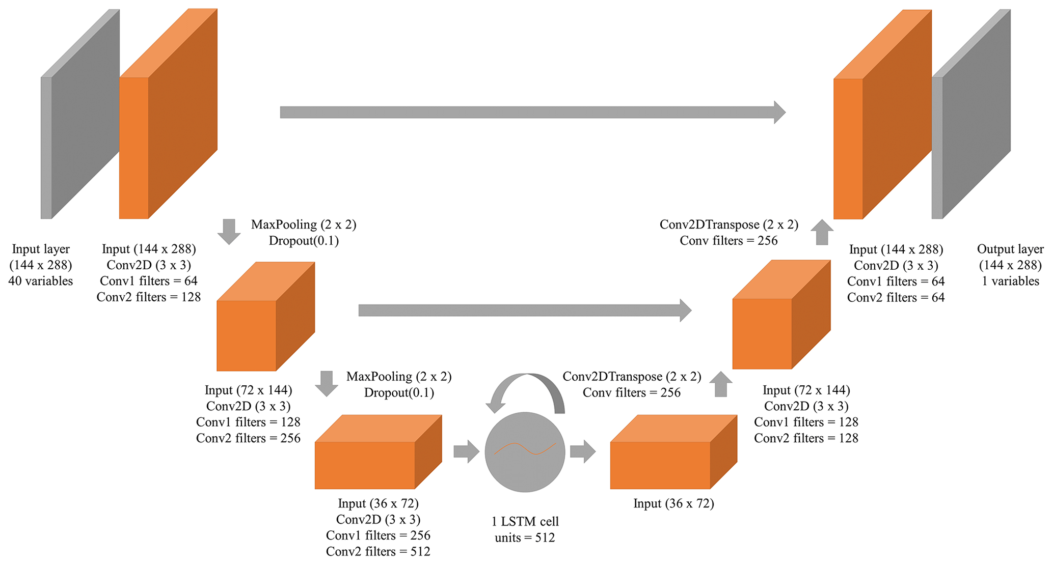
Our hyDL-CO model is a modified version of the U-net model used in He et al. (2022), where the model shows a superior capability in predicting surface summertime O₃ in North America. The U-net architecture is a variant of autoencoder and was originally proposed for biomedical segmentation applications. In the first U-net paper, Ronneberger et al. (2015) conducted three experiments and showed that the U-net model outperforms other DL models. Since the proposal of U-net, it has become one of the most popular choices in the DL community and is compared with other ML models in many studies. For example, Korznikov et al. (2021) used several ML models for tree recognition using satellite images, and the U-net model shows the highest accuracy. Ravuri et al. (2021) used U-net as a baseline model and compared it with their generative adversarial network (GAN) in precipitation nowcasting. Andersson et al. (2021) showed that their IceNet, which is an ensemble of similar U-Net networks, has outstanding performance in seasonal forecasts of Arctic Sea ice.

As shown in Fig. 1, the first three blocks of neural layers behave as an encoder, which has six convolutional layers and two max pooling layers, to extract the features hidden in the input data. A dropout layer is added after each pooling layer to prevent data overfitting. The output from the encoder is highly compressed information that is not manipulated during the training process, which is also called the latent vector. We embed the LSTM model into the U-net architecture after the encoder, inspired by the idea of convolutional LSTM proposed in Shi et al. (2015), to capture short-term changes and long-term trends in the latent vectors. The output from the LSTM is then forwarded to a decoder with three blocks of layers, which has four convolutional layers and two transposed convolutional layers. The outputs from each convolutional layer in the model are passed through the rectified linear unit (ReLU) activation function to increase non-linearity. Residual learning connections (He et al., 2016) that forward the high-resolution features extracted by the encoder to the decoder are also added, which are shown to improve the performance of U-net (Ghorbanzadeh et al., 2021; Qi et al., 2020; Liu et al., 2020). These connections contain trainable weights that represent a more direct relationship between input and output variables.

Table 1 Hyperparameters used in the hybrid DL model.

The optimization of the model is supervised by the “ground truth”, which is the daily mean surface CO concentrations measured by the MEE network. The weights in the CNNs and transposed CNNs are optimized using the back-propagation algorithm (Rumelhart et al., 1986; LeCun et al., 1989), which employs the partial derivatives of the cost function with respect to the truth. Here cost function is defined as follows:

$$\begin{array}{}\text{(4)}& L={\displaystyle \frac{\mathrm{1}}{N}}\sum _{i=\mathrm{1}}^N{\left(y_i-\widehat{y_i}\right)}^{\mathrm{2}},\end{array}$$

where y_i and $\widehat{y_i}$ are the “true” and “predicted” values. This performance evaluation is calculated only in the grid with “true” values, so that the optimization of the model avoids the influence of regions without CO observations. The loss function to be optimized is the mean square error (MSE) between the “predicted” and “true” values. We use the Adam optimizer, which is a computationally efficient algorithm for gradient-based optimization of stochastic objective functions. For a faster convergence speed and the stability of the model performance, we rescale all the features to the nearly same scale. The processing method is multiplying the original variable by a constant 10ⁿ and adapting n for each variable according to the specified scale. For example, most of the values of sea level pressure (SLP) are distributed around 10⁵, so we multiply SLP by 10⁻⁴ to make the value of the feature SLP distributed around 10¹. This processing prevents the DL model from being overfit by the features in input variables that have significantly larger scales than others. The hybrid model was built and implemented using Keras and Tensorflow, which are Python packages that are extensively used in DL studies. Table 1 shows some of the configuration hyperparameters of the training of our model.

The input variables include six meteorological variables: SLP, surface incoming shortwave flux (SWGDN), 2 m air temperature (T2M), 10 m eastward wind (U10M), 10 m northward wind (V10M), total precipitation (TP), and total anthropogenic CO and volatile organic compounds (VOC) emissions. The meteorology and emission data are extracted from the GEOS-Chem model with 0.5^∘ × 0.625^∘ horizontal resolution. Our focus area is 0–72^∘ N, 0–180^∘ E, and the output resolution is same as the 0.5^∘ × 0.625^∘ resolution of MERRA-2. The DL model grid thus has 288 grid boxes along the longitudinal direction and 144 for the latitude. Considering the long lifetime of CO, the concentration of surface CO is not only related to the emission and meteorological conditions at the current moment, but also at the previous moment. We trained the DL model using the information related to the “history” of CO, by adding the same set of input variables for the current day and previous 4 d as predictors. The information from the 5 d history has 40 predictors in total for the prediction of daily mean surface CO in each day. We use 2015–2018 as the training data set and 2019–2020 as the test set. The dimension of each input vector for the DL model is then (144, 288, 40), and the dimension of the output from the DL model is (144, 288, 1).

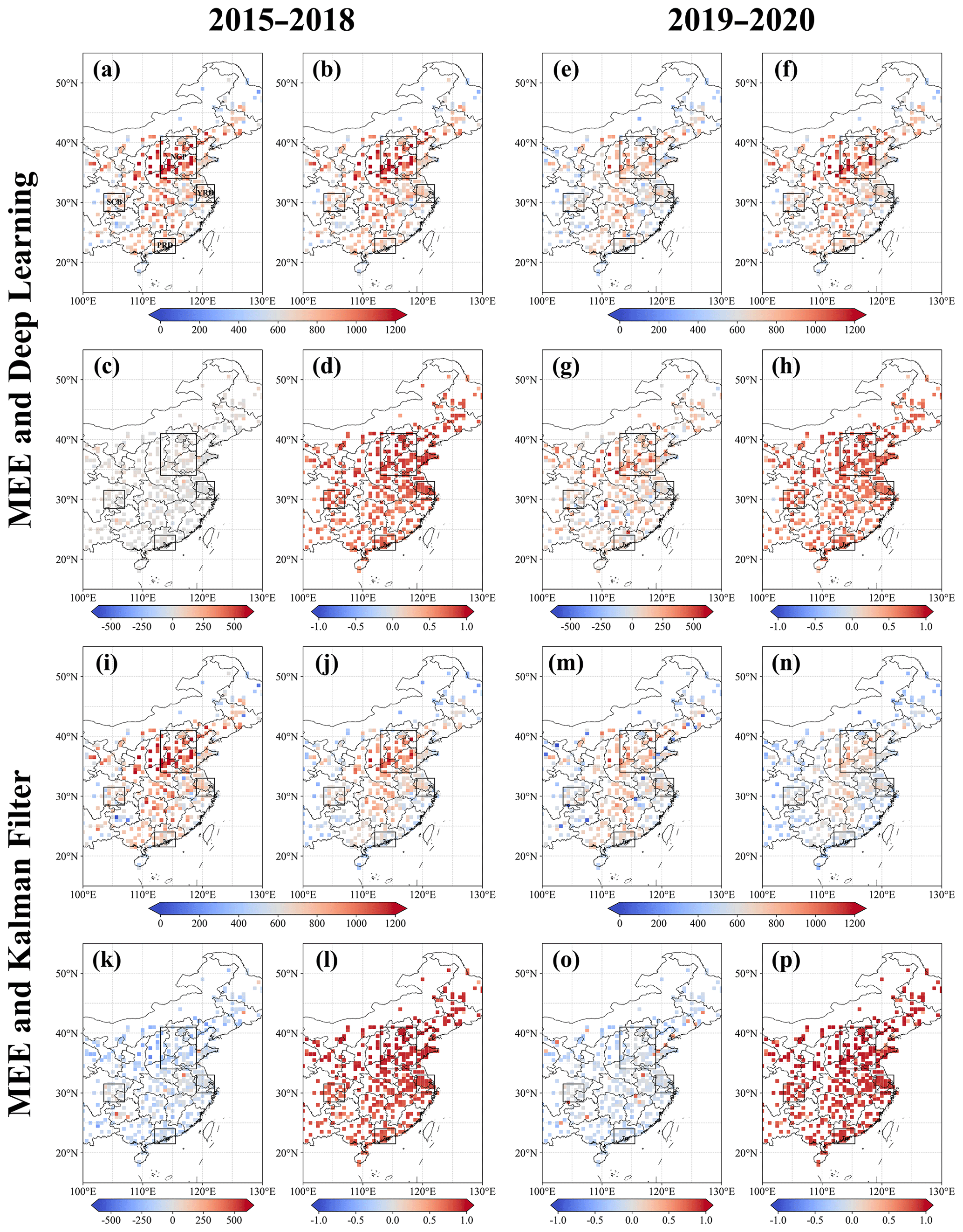
Figure 2 (a) MEE CO observations (90 % stations) in 2015–2018. (b) Predicted CO concentrations by the DL model in 2015–2018. (c, d) Differences and Pearson correlation coefficients between predicted and observed CO in 2015–2018. (e–h) MEE CO observations (90 % stations), predicted CO concentrations by DL model and their differences, and Pearson correlation coefficients in 2019–2020. (i–p) Same as panels (a–h), but for KF. The unit is ppb.

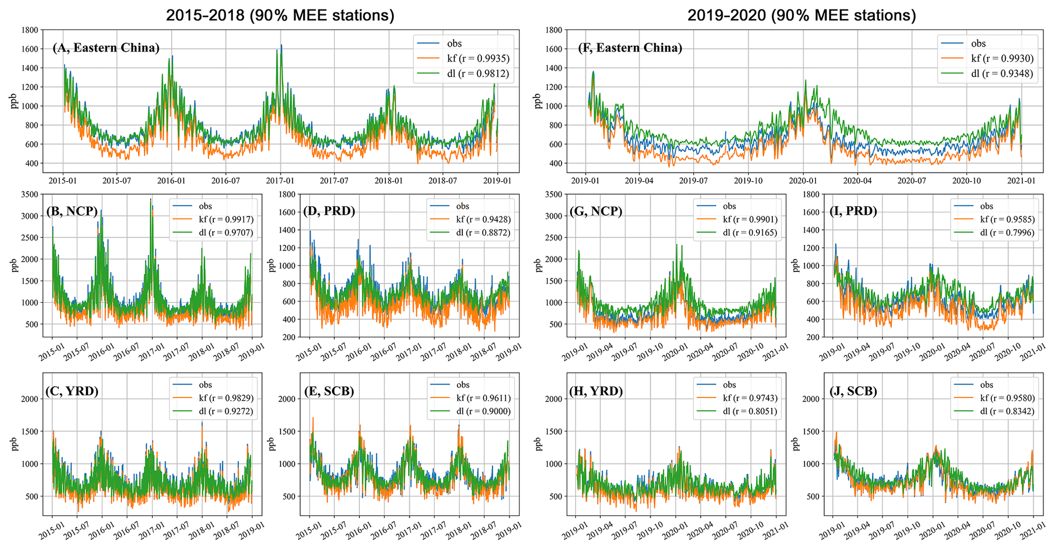
Figure 3 Daily variabilities of CO concentrations from MEE (90 % stations), DL and KF in 2015–2018 and 2019–2020.

Table 2 Deep learning (DL), Kalman filter (KF) and control run (CR) with respect to MEE CO observations in 2015–2018 and 2019–2020. The locations of independent MEE stations are shown in Fig. 6.

3 Results and discussions

3.1 CO concentrations predicted by DL model

As shown in Fig. 2a, the annual averaged MEE CO observations are broadly higher than 400 ppb in eastern China in 2015–2018 and can reach 1000 ppb over the highly polluted North China Plain (NCP). The predicted CO concentrations by the DL model (Fig. 2b) match well with observations in 2015–2018. We find small differences between predictions and observations in Fig. 2c. The Pearson correlation coefficients are larger than 0.7 over eastern China and are as high as 0.9 over the highly polluted NCP (Fig. 2d). Figure 3a–e exhibit daily variabilities of CO concentrations over eastern China, as well as NCP, Yangtze River Delta (YRD), Pearl River Delta (PRD) and Sichuan Basin (SCB) domains. There is large seasonality in the observed CO concentrations: the wintertime CO concentrations can reach 1400 ppb over eastern China and 2500 ppb over the highly polluted NCP; the summertime CO concentrations are about 500 ppb over eastern China and 800 ppb over NCP. The predicted CO concentrations by the DL model demonstrate high consistency with observations. As shown in Table 2, the correlation coefficients between the DL model and MEE CO observations are 0.98, 0.97, 0.93, 0.89 and 0.90; the biases are 9.6, 18.2, −2.6, 12.7 and 17.6 ppb for eastern China, NCP, YRD, PRD and SCB, respectively.

The high consistency between observations and the DL model in the training period (2015–2018) is expected. Here we further evaluate the capability of the DL model to predict CO concentrations without the inputs of CO observations (i.e., in the test period). Figure 2e shows the MEE CO observations in 2019–2020. As shown in Fig. 2f, the DL model overestimated surface CO concentrations in 2019–2020, particularly, over the highly polluted NCP. The Pearson correlation coefficients in 2019–2020 (Fig. 2h) are slightly lower than those in the training period (Fig. 2d). As shown in Fig. 3f, the predicted CO concentrations exhibit larger deviations from observations in 2019–2020. The correlation coefficients (see Table 2) between observed and predicted CO in the test period are 0.93, 0.92, 0.81, 0.80 and 0.83; the biases are 95.7, 224.2, 22.0, 60.8 and 52.8 ppb for eastern China, NCP, YRD, PRD and SCB, respectively. Consequently, the lack of inputs of CO observations in the test period led to a decline of prediction capability, but it is still high enough to provide useful information to predict CO variabilities.

3.2 Changes of CO emissions inferred by DL model

Here we further explore the possible sources for the deviations of predicted CO concentrations from observations in 2019–2020. The observed CO concentrations are about 640 ppb in the summer of 2015 and decreased gradually to about 620 ppb by the summer of 2018. However, the observed CO concentrations dropped to about 550–530 ppb in the summer of 2019 and 2020. The rapid decrease in surface CO concentrations is dominated by the highly polluted NCP (Fig. 3g), whereas the differences between predicted and observed CO concentrations are limited over other domains. The rapid decrease in surface CO concentrations over NCP in 2019 could be associated with an unexpected drop in CO emissions, which is not considered in the linear projection of emission inventory, and led to overestimated CO concentrations in the DL model. In addition, recent studies (K. Li et al., 2020; X. Chen et al., 2021) indicated a dramatic increase in surface O₃ concentration over NCP in 2019. The possible changes in atmospheric oxidation capability and sink of CO may not be sufficiently captured by the DL model, as the relevant information is not used as the input while training the model.

The unprecedented lockdowns across the world to contain the 2019 novel coronavirus (COVID-19) spread have led to a slowdown of economic activities, with pronounced declines in anthropogenic emissions. Shi and Brasseur (2020) found surface CO concentrations over northern China were 1.2–1.5 and 0.7–1.0 mg m⁻³ before and during the pandemic spread. Gaubert et al. (2021) suggested a reduction of about 15 % in CO emissions over northern China due to the COVID-19 controls. As shown in Fig. 3f, the MEE CO observations are about 10.2 % and 25.8 % lower than predicted CO by the DL model in Feb 2019 and 2020, respectively; the MEE CO observations are about 11.1 % and 14.2 % lower than predicted CO by the DL model in June–August 2019 and 2020, respectively. Assuming the difference in June–August (i.e., 11.1 % and 14.2 %) represents the annual CO emission trends, our analysis thus suggests a decline of about 12.5 % in CO emissions caused by COVID-19 controls, which is consistent with Gaubert et al. (2021).

3.3 Comparison between the DL model and KF assimilation

Figure 2i–p show the MEE CO observations and assimilated CO concentrations by KF in 2015–2018 and 2019–2020. In contrast to the DL approach, CO observations are assimilated in KF in both periods. While the spatial distributions of assimilated CO match well with observations, the CO concentrations in the assimilations are noticeably lower. As shown in Fig. 3a–e and Table 2, the differences between assimilated and observed CO are −114.9, −139.6, −58.0, −108.8 and −29.3 ppb for eastern China, NCP, YRD, PRD and SCB, respectively, which are larger than the differences in the DL model. Furthermore, the modeled CO concentrations in the control runs (CR, without assimilation of CO observations) are much lower: the differences are −409.6, −512.3, −246.0, −400.5 and −172.4 ppb for eastern China, NCP, YRD, PRD and SCB, respectively. The dramatic underestimations of CO concentrations in model simulations have been reported in recent studies (Feng et al., 2020; Kong et al., 2020; Peng et al., 2018), which could be associated with significant model representation error because most MEE stations are urban sites (Tang et al., 2022). It reveals the important discrepancy between DL and data assimilations: the analyzed concentrations in KF are based on the a priori and observed concentrations by considering the model and observation errors, which are not designed to reproduce the observations. In addition, the correlation coefficients are 0.99, 0.99, 0.98, 0.94 and 0.96 for eastern China, NCP, YRD, PRD and SCB in 2015–2018 in the KF, respectively, which are comparable with the DL model.

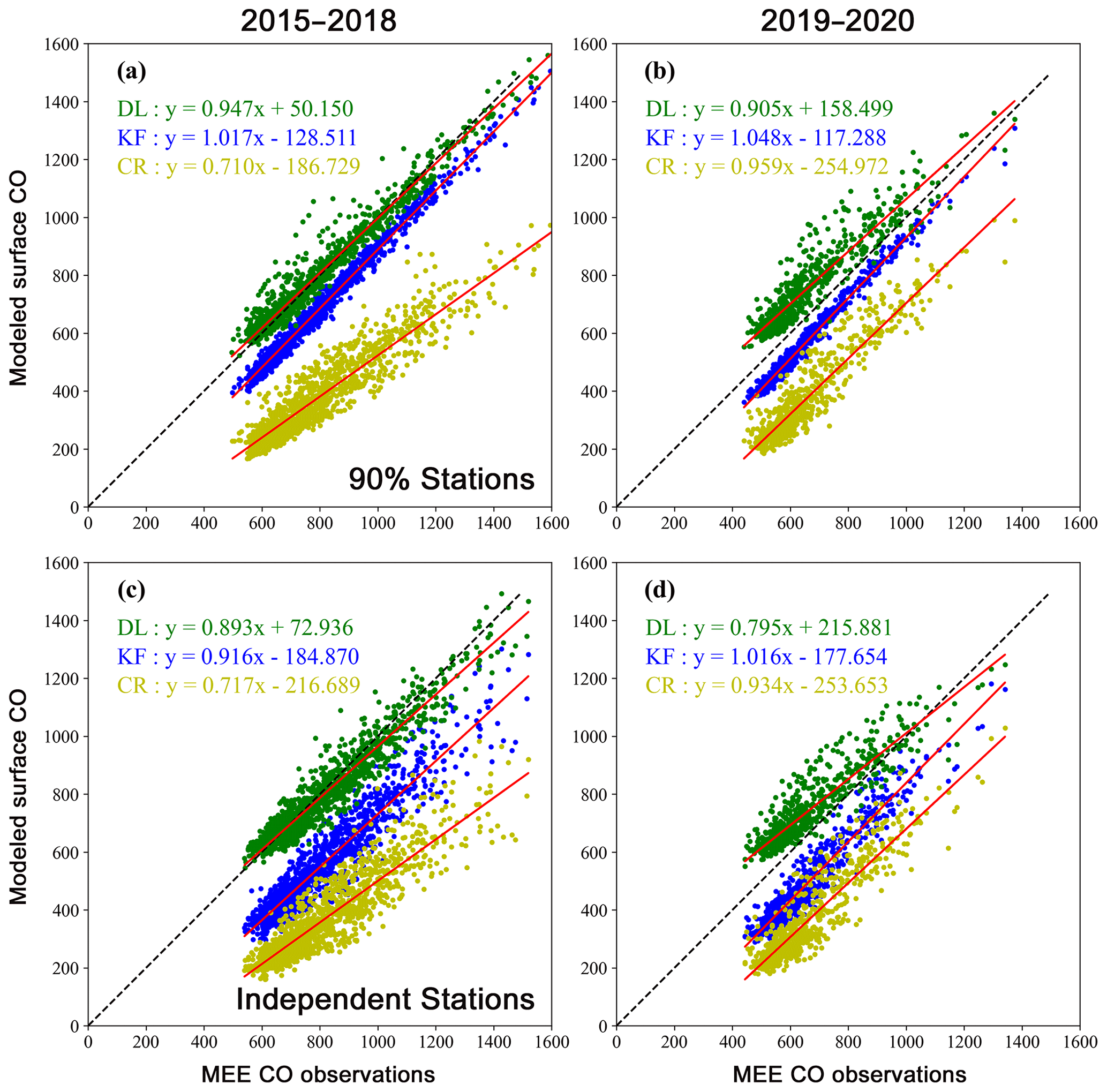
Figure 4 (a, b) Relationships between CO concentrations provided by DL, KF, control run (CR) and MEE CO observations in 2015–2018 and 2019–2020. The dots represent daily average of CO concentrations over eastern China. The unit is ppb. (c, d) Same as panels (a, b), but with randomly selected independent MEE stations. The locations of independent MEE stations are shown in Fig. 6.

As shown in Fig. 3f–j and Table 2, the differences between assimilated and observed CO concentrations in 2019–2020 are −85.5, −66.3, −52.9, −89.3 and −18.7 ppb for eastern China, NCP, YRD, PRD and SCB, respectively, which are comparable with the differences in the DL model except for the highly polluted NCP; even the MEE CO observations are not inputted in the DL model in the test period. The correlation coefficients are 0.99, 0.99, 0.97, 0.96 and 0.96 for eastern China, NCP, YRD, PRD and SCB in 2019–2020 in the KF, respectively, which are higher than the DL model. In addition, Fig. 4a and b show the relationships between modeled CO and MEE CO observations. Both DL and KF show dramatic improvements with respect to the CR simulations in Fig. 4a and b, while the performance of the DL model is better than KF in the training period (Fig. 4a). In addition, the comparable performances between DL and KF in 2019–2020 (Fig. 4b) demonstrate the good temporal extensibility of DL model; i.e., skills learned in the training period can be extended to the following years with a limited decline in the prediction effects.

Figure 5 (a, b) Predicted by DL (contour) and MEE (dotted) surface CO concentrations in 2015–2018 and 2019–2020. (c, d) Same as panels (a, b), but for KF.

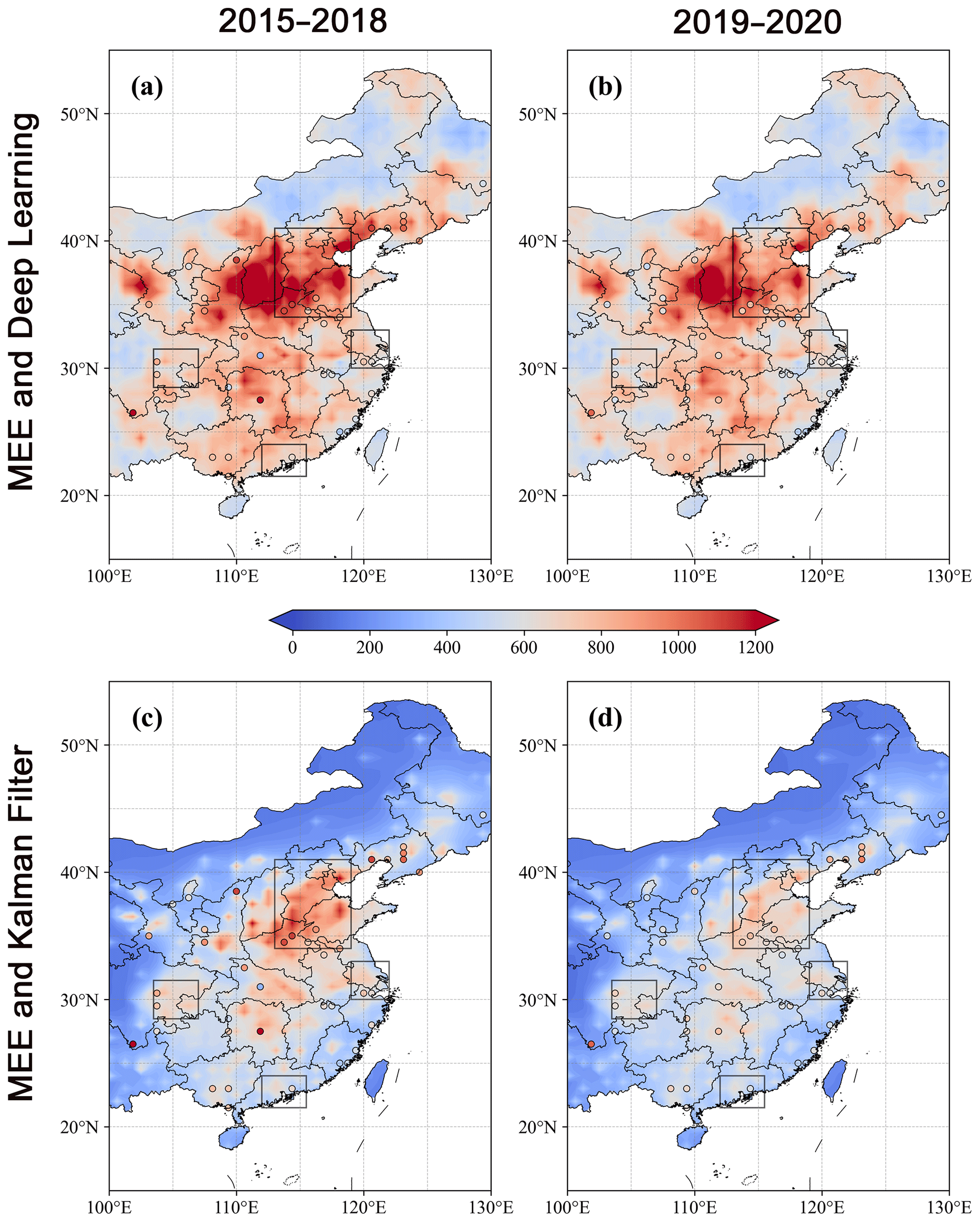
Figure 6 (a, b) Predicted by DL (contour) and independent MEE (dotted) surface CO concentrations in 2015–2018 and 2019–2020. (c, d) Same as panels (a, b), but for KF. The randomly selected independent MEE stations (about 10 % of total stations) are not used in both DL and KF in 2015–2020.

Figure 7 Daily variabilities of CO concentrations from independent MEE stations, DL and KF in 2015–2018 and 2019–2020. The locations of independent MEE stations are shown in Fig. 6.

3.4 Evaluation with independent MEE CO observations

Figure 5a and b show the spatial distributions of predicted CO concentrations by the DL model and MEE CO observations; Fig. 6a and b further exhibit the locations of randomly selected independent MEE stations (about 10 % of total stations). These independent stations are not used in either the DL model or KF in 2015–2020. Although we find broadly good agreements in the spatial distributions between predicted CO concentrations by DL and KF and MEE CO observations, there is still a noticeable discrepancy. The DL model suggests the highest CO concentrations are in the Shanxi province, by more than 1200 ppb, and background CO concentrations by about 400 ppb over remote areas. By contrast, the CO concentrations in the KF (Figs. 5c, d and 6c, d) are lower, and the highest CO concentrations are found in NCP rather than the Shanxi province. As shown in Fig. 7a–e, the DL model demonstrates a smaller bias with respect to independent MEE CO observations and higher correlation coefficients than KF in 2015–2018, suggesting better capability to predict CO concentrations. In 2019–2020 (Fig. 7f–j), the DL model exhibits a smaller bias over eastern China, but a larger bias than KF over the highly polluted NCP. The Pearson correlation coefficients are smaller in DL in 2019–2020 (see Table 2).

As shown in Fig. 4c and d, the assimilated CO concentrations by KF are closer to the control simulations with larger deviations from the MEE CO observations than those in Fig. 4a and b. It demonstrates the decline of assimilation effects when observations are unavailable. On the other hand, the slopes in the linear fits are 0.89 and 0.92 in DL and KF in 2015–2018 (Fig. 4c), respectively, and become 0.80 and 1.02 in 2019–2020 (Fig. 4d). The deviations in the slopes reflect an underestimation of CO concentrations in the DL model at grids with extremely high CO concentrations. The DL model predicts CO concentrations based on the skills learned in the training process. However, the training is dominated by the majority of CO observations with low and medium CO concentrations. As shown in Fig. 4a and b, extreme pollution events, with CO concentrations > 1200 ppb, account for only 3.4 % of the total number of observations. It cannot be learned sufficiently, because the DL model, as a data-driven approach, would require more observations about the extreme pollution events to improve the predictions. By contrast, KF is driven by observations directly so that both high and low CO concentrations can be simulated. In addition, because most MEE stations are urban sites, the good agreement between the DL model and MEE CO observations may not be able to ensure the accuracy of predicted CO concentrations over remote rural areas, as well as the high CO concentrations over mountain areas around urban basins in the Shanxi province. Integration of modeled CO concentrations in the DL model in future studies may improve predicted CO concentrations over remote areas without local observations.

4 Conclusion

A hybrid DL model (hyDL-CO), based on CNN and LSTM, was built in this work to provide a comparative analysis between DL and KF to predict CO concentrations in China in 2015–2020. We find the performance of the DL model is better than KF in the training period (2015–2018): the bias and correlation coefficients are 9.6 ppb and 0.98 over eastern China and −12.5 ppb and 0.96 over grids with independent observations. By contrast, the assimilated CO concentrations by KF demonstrate comparable correlation coefficients but larger negative biases: the bias and correlation coefficients are −114.9 ppb and 0.99 over eastern China and −252.5 ppb and 0.95 over grids with independent observations. The larger biases in the KF are caused by the discrepancy in the algorithm; i.e., the objective of data assimilation is to improve the simulated atmospheric compositions by considering the model and observation errors, which are not designed to reproduce the observations. Both DL and KF show better predictions than the control runs: the bias and correlation coefficients are −409.6 ppb and 0.94 over eastern China and −443.3 ppb and 0.91 over grids with independent observations.

Furthermore, we find good temporal extensibility of the DL model in the test period (2019–2020): the bias and correlation coefficients are 95.7 ppb and 0.93 over eastern China and 81.0 ppb and 0.91 over grids with independent observations. The correlation coefficients (0.91–0.93) show there is enough capability to provide useful information to predict CO variabilities without inputs of CO observations. In addition, we find an unexpected drop in CO emissions over the highly polluted NCP in 2019. Our analysis further exhibits a significant decline in CO emissions in early 2020 due to the COVID-19 controls. Despite these advantages, we find a noticeable underestimation of CO concentrations at grids with extremely high CO concentrations in the DL model, because the training is dominated by the majority of CO observations with low and medium CO concentrations, and thus the extreme pollution events cannot be learned sufficiently. This work demonstrates the advantages and disadvantages of DL models to predict atmospheric compositions with respect to traditional data assimilation. We assume comparable or better performances of DL in the predictions of O₃ and PM_2.5 than the CO analysis shown in this work, because of their shorter lifetimes, and advise more efforts to explore new applications of DL models in the predictions of other atmospheric compositions.