The Regional Coupled Suite (RCS-IND1): application of a flexible regional coupled modelling framework to the Indian region at kilometre scale

A new regional coupled modelling framework is introduced – the Regional Coupled Suite (RCS). This provides a flexible research capability with which to study the interactions between atmosphere, land, ocean, and wave processes resolved at kilometre scale, and the effect of environmental feedbacks on the evolution and impacts of multi-hazard weather events. A configuration of the RCS focussed on the Indian region, termed RCS-IND1, is introduced. RCS-IND1 includes a regional configuration of the Unified Model (UM) atmosphere, directly coupled to the JULES land surface model, on a grid with horizontal spacing of 4.4 km, enabling convection to be explicitly simulated. These are coupled through OASIS3-MCT libraries to 2.2 km grid NEMO ocean and WAVEWATCH III wave model configurations. To examine a potential approach to reduce computation cost and simplify ocean initialization, the RCS includes an alternative approach to couple the atmosphere to a lower resolution Multi-Column K-Profile Parameterization (KPP) for the ocean. Through development of a flexible modelling framework, a variety of fully and partially coupled experiments can be defined, along with traceable uncoupled simulations and options to use external input forcing in place of missing coupled components. This offers a wide scope to researchers designing sensitivity and case study assessments. Case study results are presented and assessed to demonstrate the application of RCS-IND1 to simulate two tropical cyclone cases which developed in the Bay of Bengal, namely Titli in October 2018 and Fani in April 2019. Results show realistic cyclone simulations, and that coupling can improve the cyclone track and produces more realistic intensification than uncoupled simulations for Titli but prevents sufficient intensification for Fani. Atmosphere-only UM regional simulations omit the influence of frictional heating on the boundary layer to prevent cyclone over-intensification. However, it is shown that this term can improve coupled simulations, enabling a more rigorous treatment of the near-surface energy budget to be represented. For these cases, a 1D mixed layer scheme shows similar first-order SST cooling and feedback on the cyclones to a 3D ocean. Nevertheless, the 3D ocean generally shows stronger localized cooling than the 1D ocean. Coupling with the waves has limited feedback on the atmosphere for these cases. Priorities for future model development are discussed.

1 Introduction

There is a growing focus from researchers around the world on the potential of more integrated coupled approaches to environmental prediction on regional scales. A key driver for this development is to provide more accurate forecasts and warning of natural hazards and their impacts, focusing where multiple hazards occur concurrently and where representing the effect of air–sea interactions impacts the evolution of high-impact weather systems. The application of regional coupled models is gaining attention to improve simulations focussed on both short-term operational natural hazard prediction (e.g. Ruti et al., 2020) and longer-timescale assessments of environmental change (e.g. Gutowski et al., 2020).

This paper describes a new kilometre-scale atmosphere–land–ocean–wave coupled system designed to support research on the sensitivity of environmental predictions in the Indian region to the representation of interactions and feedbacks between model components. As reviewed by Hagos et al. (2020), the application of atmosphere–ocean coupled systems in tropical regions is particularly relevant given that air–sea interactions drive and can impact tropical meteorological processes. Recent studies have highlighted the sensitivity of environmental processes in the Indian region to interactions between different components of the environment. For example, Roman-Stork et al. (2020) examined reanalysis products to demonstrate that reduced transport of fresher water from the Bay of Bengal over the past 15 years, fed by river discharge, has increased the depth of a barrier layer in the south-eastern Arabian Sea, in turn contributing to a reduction in the number of intense monsoons. Salinity–precipitation feedback mechanisms were also explored by Krishnamohan et al. (2019), who focussed on more localized processes in the Bay of Bengal. Karmakar and Misra (2020) found propagation of the summer monsoon rainfall to be faster over the Arabian Sea than the Bay of Bengal due to a relative enhancement of convection over the Arabian Sea associated with moisture convergence.

On shorter timescales, the importance of air–sea interaction in modulating the evolution of tropical weather systems is also well known. This is most clearly illustrated for tropical cyclones (TCs) that are prevalent within the Bay of Bengal, and there is a notably high number of studies published on this topic in recent years. For example, TC Vardah (December 2016) was shown to be sensitive to atmosphere–wave coupling and the inclusion of dynamic sea spray flux in the COAWST system of Warner et al. (2010) (Prakash et al., 2019) and to atmosphere–ocean mixed layer coupling, with sensitivity depending on initial mixed layer depth (Yesubabu et al., 2020). The sensitivity of TC simulations using a regional coupled model were found to be highly sensitive to the surface drag parameterization by Greeshma et al. (2019). Mohanty et al. (2019) quantified improvements in TC position and timing errors of 20 % and 33 % respectively for HWRF (Biswas et al., 2018) atmosphere model simulations of several TCs in the Bay of Bengal when applying 6-hourly updating SST boundary conditions compared to a control simulation in which the SST conditions persist through the simulations. This latter approach is typical of regional modelling configurations used in most operational NWP centres (e.g. Routray et al., 2017; Mahmood et al., 2021). The relevance of spatial resolution of SST boundary conditions for atmosphere-only simulation of TC Phailin was examined by Rai et al. (2019), who found improved performance of the order of 30 %–40 % when using a higher-resolution (0.083^∘ × 0.083^∘) SST analysis.

Beyond the well-documented impacts of TC multi-hazards on lives and livelihoods (e.g. Pandey et al., 2021), the impact of TCs on physical and biogeochemical ocean processes in the Bay of Bengal are also receiving increasing attention. For example, Maneesha et al. (2019) and Girishkumar et al. (2019) discussed the observed impact of TC Hudhud on upper ocean dynamics and chlorophyll a, finding this was maintained for 2 weeks after the passage of the storm. The impact of TC Phailin on the upper ocean was assessed by Jyothi and Joseph (2019) and Qiu et al. (2019) in different ocean-only simulations, building on the earlier COAWST coupled model assessment of this case by Prakash and Pant (2017). The signature cooling of the ocean mixed layer by as much as 7 ^∘C in response to the passage of the TC was noted, in addition to strong TC-induced upwelling and substantial increases of up to 5 psu in surface salinity over these regions. Maneesha et al. (2021) highlighted the considerable impacts that TCs can have on marine biogeochemistry in the region but noted relatively limited impacts of TC Titli due to persistent stratification in western regions suppressing upwelling.

This paper aims to document the first implementation of a regional coupled modelling system focussed on the Indian region that uses the Unified Model atmosphere, JULES land surface, NEMO or Multi-Column K-Profile Parameterization (KPP) ocean and WAVEWATCH III wave model codes. The modelling framework described in this paper is defined to run at kilometre scale across all components (4.4 km atmosphere, 2.2 km ocean), to enable explicit representation of key processes including atmospheric convection (e.g. Turner et al., 2019; Volonté et al., 2020) and ocean eddies and internal tides within shelf seas (e.g. Jithin et al., 2019). This resolution also offers the potential to represent catchment-scale hydrology and land–sea interactions at coastlines with better fidelity than typically possible with regional and global-scale coupled model approaches running with grid resolutions of the order of 10 km or coarser (e.g. Eilander et al., 2020). This represents a marked increase in spatial resolution relative to most coupled modelling studies highlighted above for the region that tend to be based on atmosphere (typically WRF; Skamarock et al., 2008) and ocean (typically ROMS; Shchepetkin et al., 2005) simulations running of the order of 10 km resolution or coarser, for which atmospheric convection is parameterized. Furthermore, there has been relatively little assessment of the role of wave processes in modifying the air–sea interactions under extreme conditions such as TCs in previous modelling studies. The option of using a lower horizontal resolution KPP ocean mixed layer parameterization component is also introduced here to examine the performance of a computationally cheaper coupled configuration relative to the 2.2 km resolution 3D general ocean circulation model with a full dynamical ocean representation.

The rest of this paper is organized as follows. Section 2 describes the RCS-IND1 definition of the RCS modelling framework and its component configurations. Section 3 provides an initial assessment of system performance and the impact of coupling for case study simulations of cyclones Titli and Fani which developed in the Bay of Bengal during October 2018 (post-monsoon) and April 2019 (pre-monsoon) respectively. Future development priorities are finally outlined in Sect. 4.

2 The RCS-IND1 implementation of the Regional Coupled Suite prediction framework

The first version of the India-focussed implementation of the RCS, termed RCS-IND1 for brevity, builds on the development of a regional environmental prediction system using the same model components and grid resolutions focussed on the north-west European shelf region (UKC; Lewis et al., 2019, 2018). RCS-IND1 incorporates atmosphere, land surface, ocean and wave model components. Coupling between required components is achieved with the OASIS3-MCT (Ocean Atmosphere Sea Ice Soil) coupling libraries (version 2.0; Valcke et al., 2015). Configurations of the following model codes are included:

• Unified Model (UM) atmosphere (version 11.1; e.g. Brown et al., 2012);

• Joint UK Land Environment Simulation (JULES) land surface model (version 5.2; Best et al., 2011; Clark et al., 2011);

• Nucleus for European Models of the Ocean (NEMO) 3D ocean model (version 4.0.1; NEMO team, 2019);

• Multi-Column K-Profile Parameterization (KPP) 1D ocean model (version 1.0; Hirons et al., 2015);

• WAVEWATCH III surface wave model (version 4.18; WW3DG, 2016).

As described below, some code modifications are applied to the referenced versions for use in the RCS-IND1 configuration, mainly related to optimization, introduction of coupling capability, or enabling additional diagnostic output. The UM and JULES models are compiled as a single executable, with implicit coupling between the land and atmosphere using the coupling methodology of Best et al. (2004) for each model time step, rather than via the OASIS-MCT coupler.

2.1 Model domain

The model domain illustrated in Fig. 1 covers the region 3.5–40^∘ N and 65–101^∘ E. This is selected to be comparable to the extent and grid resolution of the NCUM-R operational atmosphere configuration (Jayakumar et al., 2017; Mamgain et al., 2018; Jayakumar et al., 2019) and operational coastal ocean and wave modelling capabilities (e.g. Francis et al., 2021; Remya et al., 2022). The benefit of building on the NCUM-R domain is that potential atmosphere model issues, for example those related to steep Himalayan orography, have previously been considered and addressed.

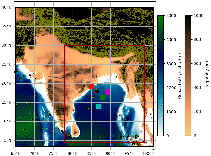
Figure 1 Illustration of RCS-IND1 domain coupled system domain extent. Shaded contours represent the atmosphere model orography over land and ocean model bathymetry respectively. Orography contours for land higher than 1000 m (black shading) are marked every 1000 m. The region highlighted by the maroon box shows the region of focus for results presented in this paper. Marked locations indicate in situ observation points referred to in the results section: from north to south, red shows Gopalpur (84.9^∘ E, 19.3^∘ N), magenta shows 23091 (89.2^∘ E, 17.8^∘ N), green shows 23093 (88.0^∘ E, 16.3^∘ N), and blue shows 23459 (87.0^∘ E, 14.0^∘ N).

Relative to the NCUM-R atmosphere domain, the RCS-IND1 coupled system domain is marginally extended to the east to cover the whole ocean extent of the Malacca strait. The appropriate location for the southern domain boundary was considered, given the importance of the south-west monsoon current in exchanging water between the Bay of Bengal and Arabian Sea (e.g. Schott and McCreary, 2001) and of the equatorial currents further south (e.g. Sanchez-Franks et al., 2019). On balance, it was considered preferable to follow the approach of the operational regional ocean model development by the Indian National Centre for Ocean Information Services (INCOIS; e.g. Francis et al., 2021) in limiting the southern domain extent to 3.5^∘ N with the assumption that this was sufficiently far south to capture much of the monsoon current and sufficiently far north that the equatorial currents could be better captured through lateral boundary conditions, rather than being partially included in the domain, or needing to extend the atmosphere and ocean domain size across the Equator as far as order 3–5^∘ S.

The ocean and wave components extend across all sea areas of the coupled model domain (Fig. 1). Note that sea grid points in the Gulf of Thailand to the far east of the domain are masked in the ocean and removed in the wave model, so that ocean and wave calculations do not take place in this region.

2.2 Coupling framework

The RCS is built as a rose suite (http://metomi.github.io/rose/doc/html/index.html, last access: 27 October 2021) that defines the component configurations and methods for running simulations. Models are run with daily cycling, whereby every cycle after the first day uses the final state of the previous cycle to re-initialize. Details of component initialization are provided further below. The flexibility of the RCS results from it being possible to run one of multiple different coupled and uncoupled configuration options (Fig. 2), based on the setting of a RUN_MODE environment variable specified from within the same rose suite (see Tables 1 and 2). This flexibility prevents the need to develop and maintain different suites for different run options (e.g. as in Lewis et al., 2018, 2019). The main modes of running simulations are as follows:

• Fully coupled (RUN_MODE = atm-ocn-wav): two-way feedbacks represented between all model components in the system (Table 1).

• Partially coupled (RUN_MODE = atm-ocn, atm-kpp, atm-wav, or ocn-wav): two-way feedbacks represented between only two selected components (Table 1).

• Uncoupled (RUN_MODE = atm, ocn, or wav): no coupled feedbacks with external components are represented, but model components can be configured with different forcing options (Table 2).

Surface boundary conditions are provided via file forcing when not available via coupling, such as when running in partially coupled or uncoupled mode. Different choices for the source of file forcing data can be specified in the RCS as environment variables prior to a model run (see Tables 3–5), which are pre-processed as part of the suite workflow during run time given the location of the source data.

Table 1 Summary of the RCS-IND1 fully and partially coupled configurations available within the RCS, and naming conventions used in this paper. Options are controlled in the RCS using the RUN_MODE environment variable. Results for configuration names in bold are demonstrated in this paper. See also Fig. 2.

Table 2 Summary of the RCS-IND1 uncoupled configurations available in the RCS, and naming conventions used in this paper. Results from configuration names in bold are demonstrated in this paper. Options are controlled in the RCS using the RUN_MODE environment variable. See also Fig. 2.

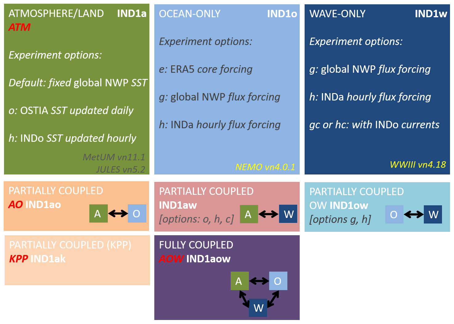
Figure 2 Schematic summary of RCS-IND1 modelling framework configuration, experiment options and naming conventions. Configurations highlight with experiment identifiers in red are presented in this paper.

The KPP ocean component is only currently supported in the suite to run in atmosphere–KPP coupled mode, and therefore no additional forcing is necessary. Tables 1 and 2 summarize all currently available research configurations of the RCS modelling framework, which are illustrated in Fig. 2, along with the associated naming convention introduced to support a variety of potential experimental designs. Not all possible configurations will be further discussed in this paper for simplicity.

Namelists defining all the available RCS-IND1 configurations are provided under the rose framework as suite u-bf945, accessible to registered researchers under a repository at https://code.metoffice.gov.uk/trac/roses-u/browser/b/f/9/4/5/trunk (last access: 30 May 2022). A more detailed description of the namelists used for each configuration is included in the Supplement to this paper.

The exchange of model variables between each coupled component and their required order of coupling (Table 3) have previously been described in detail for the UKC2 and UKC3 regional coupled systems (Lewis et al., 2018, 2019), although there are some minor differences in the fields that are now exchanged. When coupling the ocean to the wave model (with or without coupling to the atmosphere model), components of the water-side stress vector transmitted into the ocean are exchanged from the wave to the ocean model, rather than in the previous approach where the fraction of the atmospheric momentum transferred to the ocean was exchanged (i.e. Eq. 3 of Lewis et al., 2019). The surface momentum budget can be expressed as follows:

$$\begin{array}{}\text{(1)}& {\mathit{\tau }}_{\mathrm{oc}}={\mathit{\tau }}_{\mathrm{atm}}-{\mathit{\tau }}_{\mathrm{wav}}+{\mathit{\tau }}_{\mathrm{wav}:\mathrm{ocn}},\end{array}$$

where τ_oc is the atmospheric stress transmitted into the ocean, τ_atm is the stress applied by the atmosphere on the ocean surface, τ_wav is the momentum flux absorbed by the wave field, and τ_wav:ocn is the momentum stored by waves that is transferred to the ocean through wave breaking. Options to further simplify and enhance the representation of the near-surface momentum budget across a three-way-coupled system are under investigation. The first change to exchanging components rather than a fractional momentum transfer enables a more consistent treatment of the air–sea momentum transfer across the coupled system than in UKC3, with a single derivation of the stress applied rather than these terms being recomputed in UM, NEMO and WAVEWATCH III. This helps to ensure that stress is applied in the same direction in all components. In atm-ocn-wav mode, the atmospheric stress is computed in WAVEWATCH III, derived from the 10 m wind speeds received from the atmosphere. The wave-modified stress components are then passed to NEMO. When the ocean is coupled only to the atmosphere (atm-ocn mode, no wave coupling), the water-side stress transmitted into the ocean is equal to the atmospheric momentum, and the ocean model receives these components as computed by UM/JULES and received directly via the coupler. The wind speed defined at 10 m above the ocean surface is no longer exchanged, and this parameter is only used in the ocean model when forced using the bulk formulation. Finally, although it is possible to pass the local water depth from the ocean to the wave model, this is not done in RCS-IND1, as it was found that extensive changes to the wave code running for SMC wave grids would be required to enable this exchange. This issue will be revisited in future in the context of updating the WAVEWATCH III code.

All coupling fields are computed as hourly mean values and exchanged every hour of the simulation starting from the initialization of the models (time step zero). A series of experiments using the UKC3 mid-latitude domain determined that increasing the coupling frequency from an hour to every 10 min did not substantially impact results in that domain, but this will need to be revisited for the RCS-IND1 tropical domain to better represent timescales for changing conditions in squalls and tropical cyclones.

2.3 Atmosphere and land surface components

The atmosphere and land surface components in RCS-IND1 have a fixed-resolution latitude–longitude grid with horizontal grid spacing of 4.4 km, which translates to 900 grid cells in the west–east zonal direction and 904 in the north–south meridional direction. They use the RAL1-T science configuration, for which science parameters and performance are described in detail by Bush et al. (2020). RAL1-T uses an 80-level terrain-following vertical coordinate set with Arakawa C-grid staggering (Arakawa and Lamb, 1977), up to 40 km altitude, with 59 levels in the troposphere below 18 km and 21 levels further above. The land surface is defined with 4 soil levels to a depth of 3 m and 9 land surface tiles to represent land surface heterogeneity within each 4.4 km wide grid cell. The integration time step for UM atmosphere and JULES land components is set to 120 s, matching the time step used in NCUM-R at the time of development (Jayakumar et al., 2021).

The initial state is taken from reconfiguration (interpolation) of a global-scale UM analysis for a given initialization time. For the experiments described in this paper, these are provided by the operational analysis used for Met Office global numerical weather prediction (Walters et al., 2019; Sharma et al., 2021), which was running with a horizontal grid resolution of the order of 17 km at tropical latitudes at the time of Titli and Fani cases. Horizontal boundary conditions are provided by re-running simulations of that global UM configuration. Given the extended length of case study simulations considered here, those global UM simulations were re-initialized from a new analysis each day through a case study, such that lateral boundary conditions were no more than 24 h beyond a new analysis time.

Optimization and coupling modifications were added to the UM version 11.1 reference code for RCS-IND1, in order to

• activate wave coupling capabilities independently of ocean coupling,

• add OMP barriers (OpenMP) to avoid threads accessing the same memory without proper synchronization (data race), and

• adjust the bounds of some loops and how coordinate sentences are written between OMP threads.

The following code changes were also introduced in JULES version 5.2:

• introduction of a variable Charnock parameter at each grid point,

• improved convergence stability in the calculation of the Obukhov length.

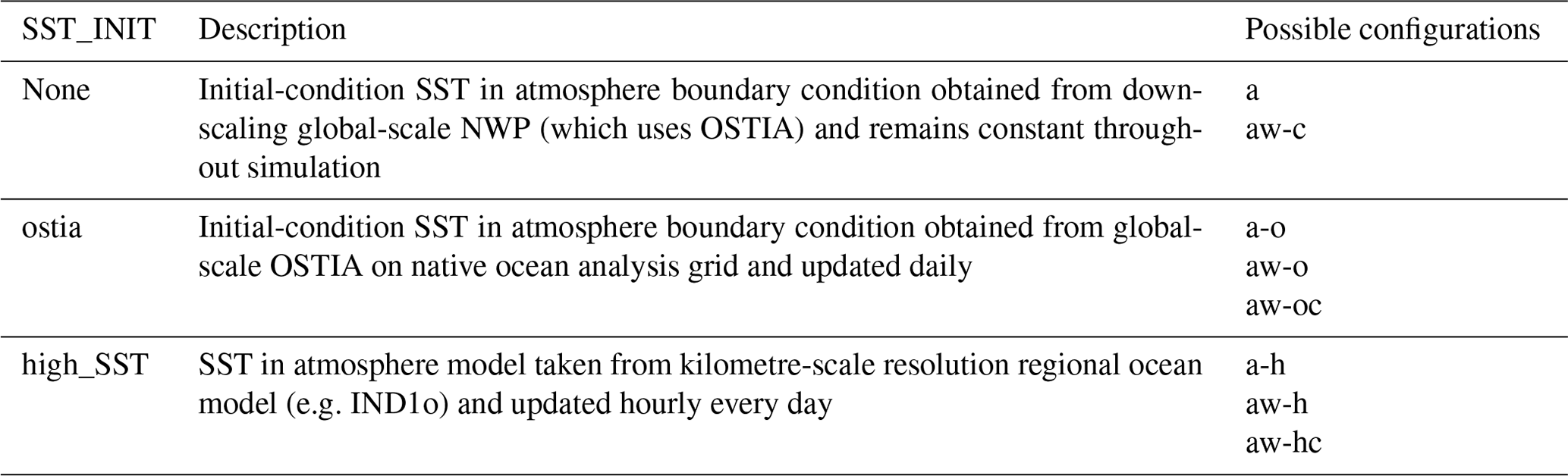
When run without ocean coupling, different approaches are supported in the RCS to define how the sea surface temperature (SST) is applied as a lower boundary condition to the atmosphere component, controlled by SST_INIT and SST_REINIT environment variables (Table 4):

• Initial-condition SST is read either from a global UM analysis (SST_INIT = none), which uses the OSTIA analysis (Donlon et al., 2012) available at the time of its creation and mapped onto the global UM grid or from reading OSTIA data directly on its native 0.05^∘ grid (SST_INIT = ostia). This initial-condition SST is either kept constant for the duration of a simulation (the default) or can be updated daily through the run (set if SST_REINIT = true).

• Initial-condition SST is interpolated from kilometre-scale resolution ocean model simulation data, e.g. the output of an ocean-only simulation of the RCS-IND1 (SST_INIT = high_sst; note not applied in this paper), and then either kept fixed or updated hourly through the run if SST_REINIT = true.

When running in uncoupled mode, surface ocean currents are assumed to be zero, and the Charnock parameter has a constant value at all ocean points of 0.011.

Table 3 Summary of the coupling exchanges between atmosphere/land (A), ocean (O), and wave (W) components within the RCS-IND1 regional coupled configuration. The fields marked with ^a are only exchanged in atmosphere/land–ocean coupled configurations. Only the fields marked with ^b are exchanged in atmosphere/land–KPP ocean coupled configurations.

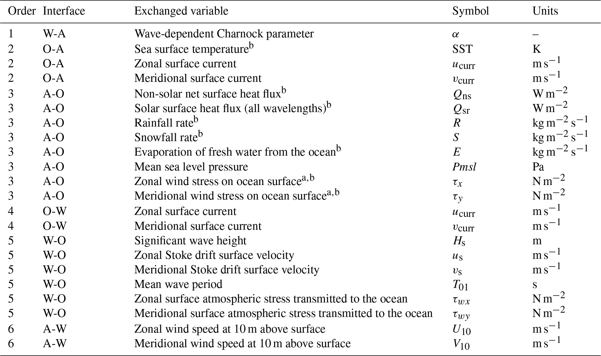
Table 4 Summary of the different SST initialization and updating options available within the RCS, applicable for model configurations in which there is no dynamic coupling to an ocean model. Options are controlled using the SST_INIT environment variable.

2.4 NEMO ocean component

The ocean component in RCS-IND1 is defined on a fixed-resolution grid with a horizontal resolution of 2.2 km (1760 grid cells in the zonal and 1100 in the meridional directions). It uses the same science configuration as used in the AMM15 ocean model developed initially for the north-west European shelf region (Graham et al., 2018; Tonani et al., 2019) and applied in the UKC regional coupled system (Lewis et al., 2019). AMM15 runs at a similar 1.5 km eddy-permitting horizontal resolution to the 2.2 km grid used for the Indian region. Some changes were applied relative to that configuration due to both updating the NEMO version from 3.6 to 4.01 and to attempt to account for specific details of the India domain:

• Integration time step is increased from 60 to 90 s. This is possible because the lower grid resolution of the RCS-IND1 model relaxes the stability conditions relative to AMM15.

• In uncoupled or ocean–wave simulations using the bulk formulation for atmospheric forcing, the Large and Yeager (2009) algorithm is substituted by the COARE 3.5 algorithm (Edson et al., 2013), as it is closer to the formulation that is used in operational implementation of AMM15 (Tonani et al., 2019).

• The formulation of the momentum advection changes from the vector form second centred scheme to the flux form third-order UBS scheme (Shchepetkin and McWilliams, 2005), as the former scheme will be removed in later versions of NEMO.

• For the RCS-IND1 configuration only one set of ocean boundary conditions is needed.

• Tidal data are read only on boundary segments, instead of assuming that each tidal data file contains all complex harmonic amplitudes.

The ocean model component has 75 vertical levels with a vertical grid using a hybrid terrain following z–s coordinate system (NEMO Team, 2019), and a non-linear free surface condition. The ocean bathymetry at 2.2 km resolution is based on the 2-Minute Gridded Global Relief Data (ETOPO2), modified to improve shallow regions (Sindhu et al., 2007). In the initial configuration described here, no river forcing is applied, which is recognized will compromise the quality of simulated ocean salinity structures. In future, it is envisaged that river flows simulated from the land component will feed into the ocean (e.g. Lewis and Dadson, 2021).

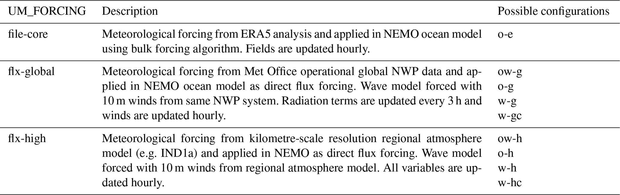
Several options for forcing the NEMO ocean model are supported when running without atmosphere coupling (Table 5):

• bulk formulation with ERA5 (Hersbach et at., 2019) input data (UM_FORCING = file-core),

• flux formulation using global atmosphere model data (UM_FORCING = flx-global),

• flux formulation using kilometre-scale resolution regional atmosphere data, such as the data produced by an atmosphere-only simulation of the RCS-IND1 configuration (UM_FORCING = flx-high).

Ocean-forced runs using the flux formulation are more easily comparable to ocean coupled runs, as the surface boundary condition forcing fields are equivalent to the coupling fields (Table 3). For more detail on the differences between the bulk and the flux forcing formulation, see NEMO team (2019).

Table 5 Summary of the different meteorological forcing options available within the RCS modelling framework, applicable for model configurations in which there is no dynamic coupling to a regional atmosphere model. Options are controlled using the UM_FORCING environment variable.

For the case studies presented in this paper, the 3D ocean state is initialized by a RCS-IND1 ocean-only simulation with ERA5 forcing starting from rest conditions on 1 January 2016, where the initial temperature and salinity profiles were obtained from the Global_Analysis_Forecast_PHY_001_024 product of the Copernicus Marine Environment Monitoring Service (CMEMS), available after registration to the Copernicus services on http://marine.copernicus.eu/ (last access: 27 October 2021). The initial temperature and salinity profiles were horizontally and vertically interpolated to the 2.2 km model grid beforehand, with coastal areas inundated and steep horizontal gradients smoothed via linear interpolation to maintain the initial stability of the run. Daily updated horizontal boundary data were obtained from the same global CMEMS product, where horizontal interpolation to the model grid is required prior to running simulations, but vertical interpolation is applied “on the fly” during simulation by a modification to the NEMO code. The rim width of the boundary data is 9 grid cells, compared to 15 in the AMM15 configuration. Tidal forcing at open boundaries takes place as a sum of five tidal constituents (M2, S2, K2, O1, K1) obtained from the FES2014 tidal model, available after registration on https://datastore.cls.fr/catalogues/fes2014-tide-model/ (last access: 27 October 2021). Further details and guidance on the workflow for the generation of the ocean component is provided by Polton et al. (2020).

Some modifications to the NEMO version 4.01 trunk source code have been made to correct issues or enable additional capabilities, as follows:

• Use the mean sea level pressure value obtained via coupling when available, instead of using a forcing file.

• Compute additional mixed layer depth diagnostics.

• Perform coupling exchanges before the initial time step of the simulation, so that the initial values of the coupling fields are available at the beginning of the run.

• Amend vertical interpolation of boundary data when the number of levels of the input boundary data is not the same as the number of levels of the model.

• Add a time stamp in the NEMO restart file name for convenience during post-processing.

2.5 Multi-Column K-Profile Parameterization (KPP) ocean component

The multi-column KPP version 1.0 code (Hirons et al., 2015) was used without modifications as an alternative approach to couple to the atmospheric model. The same regional configuration as described by Klingaman and Woolnough (2017) for the Indo-Pacific region was used in this study. By using the vertical mixing scheme of Large et al. (1994), KPP provides a computationally efficient approach to simulate one-dimensional processes such as heat fluxes in the vertical and re-distribution within the water column in the absence of horizontal advection processes. Initial conditions for temperature, salinity, and current velocity components were obtained via vertical and horizontal interpolation of the operational ORCA025 global ocean model analysis run at the Met Office (Blockley et al., 2014). Over the India-focussed domain used in this configuration (Fig. 1), the KPP component covered the same extent as the NEMO ocean component, but with a latitude–longitude horizontal grid with 0.094^∘ latitude and 0.141^∘ longitude spacing (order 15 km resolution) and 100 vertical levels. This coarser horizontal grid spacing matches the initial ocean analysis resolution (262 grid cells in the zonal and 392 in the meridional directions) and enables the 1D scheme to be applied at sufficiently coarse resolution that horizontal advection can be assumed to be neglected.

2.6 WAVEWATCH III surface wave component

The surface wave model component uses WAVEWATCH III version 4.18, using the same domain and ocean bathymetry as defined for the ocean components. The wave model uses a spherical multiple-cell (SMC) grid (Li, 2011) with 425 841 unstaggered wave grid cells with grid spacing of 2.2 km in coastal areas and expanding to 4.4 km in open seas. Some modifications were applied for RCS-IND1 to improve the support for coupling all required fields. The component applied in RCS-IND1 is the same as for the UKC3 regional coupled environmental prediction system (Lewis et al., 2019) with minor improvements detailed below:

• minor bug fixes for declaration of constant variables;

• improved initialization of coupling fields along the land/sea boundary;

• application of a cap to the coupled Charnock values larger than 0.32, to avoid spuriously high instantaneous values, noting 0.32 is an order of magnitude higher than typical climatological values.

The ST4 source term parameterization scheme (Ardhuin et al., 2010) is used in all RCS-IND1 wave configurations. The linear input source term parameterization of Cavaleri and Malanotte-Rizzoli (1981) is applied to improve initial wave growth behaviour. Non-linear wave–wave interactions are parameterized following the discrete interaction approximation (Hasselmann et al., 1985). Bottom friction is taken into account with the JONSWAP formulation (Hasselmann et al., 1973), and depth-induced breaking using the Battjes and Janssen (1978) approach. Wind and current forcing are linearly interpolated in time and space at the coarsest grid scale (4.4 km), and the wind speed forcing is corrected relative to the ocean current velocity.

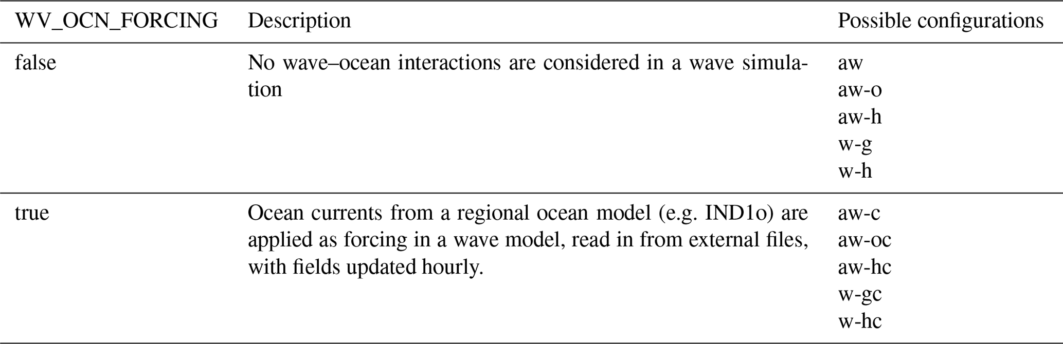
When run in uncoupled modes, the wave model can be forced (see Table 6) with ocean currents (obtained from a regional ocean model, such as the ocean-only component of RCS-IND1) and atmospheric wind, or just atmospheric wind (WV_OCN_FORCING = true/false, respectively). The atmospheric wind forcing can be provided via global NWP model data (UM_FORCING = flx-global) or regional kilometre-scale model simulations (UM_FORCING = flx-high).

Table 6 Summary of the uncoupled ocean forcing options available when running wave model configurations within the RCS modelling framework, applicable for model configurations in which there is no dynamic coupling to a regional ocean model. Options are controlled using the WV_OCN_FORCING environment variable.

The wave component in all simulations presented in this paper is initialized from a restart file generated by first running the RCS-IND1 wave-only configuration from rest for a 5 d period prior to a required case study initial time. In these spin-up simulations, wind forcing is provided by the operational global UM forecast archive, running at approximately 17 km resolution at tropical latitudes at the time of the case studies described in this paper. Spectral boundary conditions were provided from archived operational global wave model output.

3 RCS-IND1 performance and the impact of coupling: TC Titli and TC Fani case study assessment

The sensitivity of TC simulation to model coupling using the RCS-IND1 configuration has been assessed by Saxby et al. (2021) for six TCs that developed in the Bay of Bengal between 2016 and 2019. They consider RCS-IND1 performance across a range of model lead times and focus on the impact of coupling from analysis of atmosphere-only uncoupled and atmosphere–ocean coupled simulations. In this paper, the full flexibility of the RCS-IND1 framework is demonstrated for two of the cases assessed by Saxby et al. (2021), namely Cyclone Fani (April 2019; pre-monsoon, e.g. Routray et al., 2020; Zhao et al., 2020; Singh et al., 2021) and Cyclone Titli (October 2018; post-monsoon, e.g. Mahala et al., 2019; Maneesha et al., 2021). Here, the performance of a broader range of coupled simulation approaches and configuration options is considered for a single initialization time to examine the potential diversity of results.

3.1 RCS-IND1 sensitivity experiments

The different simulation approaches demonstrated in this paper for 7 d simulations of Titli (initialized at 00:00 UTC on 8 October 2018) and Fani (initialized at 00:00 UTC on 28 April 2019) cases are summarized in Table 7 (see also Fig. 2). Saxby et al. (2021) considered atmosphere-only and atmosphere–ocean coupled simulations for a variety of initialization times, but the focus on the initialization and run duration discussed here represents a balance of capturing much of each storm's life cycle and subsequent impacts. Titli formed on 8 October 2018, reaching landfall in Andhra Pradesh around 00:00 UTC on 11 October (i.e. 3 d into simulations presented here), and dissipated on 12 October. Fani was a long-lived storm, forming on 26 April 2019, 2 d prior to the initialization time assessed here, but did not reach landfall in Odisha until 02:30 UTC on 3 May 2019 (i.e. over 5 d into simulations) and dissipated on 5 May 2019, 9 d after first forming.

Table 7 Summary of naming conventions used in describing RCS-IND1 simulation experiments for Titli and Fani cases. Simulations for which frictional heating is activated in the Unified Model configuration are signified by “_FH” after the relevant run identifier. ATMfix uses fixed SST for the duration of a simulation, while ATM has daily updating SST.

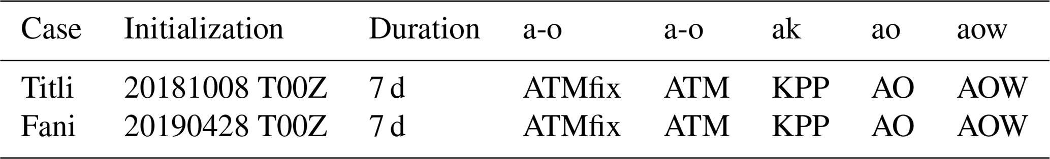
Two types of atmosphere-only control simulations are considered using the following naming conventions:

• ATMfix. Initial-condition OSTIA SST surface boundary is kept constant throughout the run of RCS-IND1a configuration,

• ATM. SST field is updated daily with the OSTIA product generated by 00:00 UTC on each day through the simulation period, to reflect the data that would have been available at that (re)-initialization time if running in near-real time.

Three approaches to representing feedbacks between atmosphere and ocean are then considered:

• KPP. The RCS-IND1ak coupled configuration is used, where the UM atmosphere component is coupled to the 1D mixed layer multi-column KPP parameterization (Sect. 2.5) each hour through the simulation.

• AO. The RCS-IND1ao configuration is used with two-way coupling between the atmosphere and the 3D NEMO ocean model component (Sect. 2.4).

• AOW. The fully coupled RCS-IND1aow configuration is run with hourly two-way coupling between atmosphere, ocean and WAVEWATCH III wave model components (Sect. 2.2; Table 3).

All simulations presented are run for 7 d from a common initial atmosphere condition, with differences of ocean and wave initial conditions described for the experiment in Sect. 2. The lateral boundary forcing at the domain edges is common across all experiments, using the same global-scale boundary conditions relevant to atmosphere, ocean and wave components.

Given the focus of application in this paper on simulation of TCs, the relative sensitivity of simulations to whether the dissipation of turbulent kinetic energy is included in the UM boundary layer parameterization is also considered. Turbulent motions are ultimately dissipated as heat, which can result in a significant contribution to the energy budget particularly at stronger wind speeds (e.g. Kilroy et al., 2017). This contribution, termed frictional heating here, is represented in the UM boundary layer parameterization following the approach of Zhang and Altshuler (1999), such that the heating rate due to dissipation can be expressed as follows:

$$\begin{array}{}\text{(2)}& {\left.{\displaystyle \frac{\partial {\mathit{\theta }}_l}{\partial t}}\right|}_{\mathrm{Dis}}={\displaystyle \frac{\mathrm{1}}{\mathit{\rho }{c}_p}}\left[{\displaystyle \frac{\mathrm{d}u}{\mathrm{d}z}}{\mathit{\tau }}_x+{\displaystyle \frac{\mathrm{d}v}{\mathrm{d}z}}{\mathit{\tau }}_y\right],\end{array}$$

with θ_l being the static energy, density ρ, specific heat of moist air at constant pressure c_p, and separated components of the vertical wind shear $\mathrm{d}\mathbf{V}/\mathrm{d}z$ and stress τ.

This term can be computed or omitted in the UM through setting a parameter option (fric_heating), which is typically enabled in global-scale model configurations running with grid spacing of order 10 km or coarser. Frictional heating is, however, typically disabled in higher-resolution regional model configurations (e.g. Bush et al., 2020) as a pragmatic approach to limiting the tendency to over-intensify strong cyclones when running convective-scale atmosphere simulations. The move towards coupled predictions and more explicit representation of air–sea interactions requires this to be re-examined. All simulations listed in Table 7 have therefore been performed without (fric_heating = 0) and with (fric_heating = 1) the frictional heating term added to the computation of sub-grid turbulent kinetic energy budget. In the current UM formulation, the additional heating is applied uniformly in the vertical over the boundary layer. Simulations with frictional heating enabled have _FH added to the respective experiment identifier when referred to in the text (e.g. ATMfix_FH for fixed SST atmosphere-only simulation with frictional heating enabled).

3.2 Impact of coupling on representation of SST

The variety of approaches to representing SST within the RCS framework is illustrated in Figs. 3 and 4 for Titli and Fani cases respectively. The ATMfix simulations exemplify the assumption imposed in most operational regional atmosphere forecasting systems, whereby the initial-condition OSTIA (representative of satellite-observed foundation SST typically 2 d prior to initialization time) persisted throughout the simulation. Note this is typically only applied over a forecast duration of a few days, for example with the NCUM-R regional forecasts currently run to 76 h (Routray et al., 2020), while the simulations used in the current case studies extend for twice as long. While only feasible for “hindcast” case study assessments rather than operational forecasting, the ATM simulations in Figs. 3d and 4d show the Bay of Bengal sub-region mean OSTIA SST becomes around 0.5 K cooler when applying daily updating OSTIA SST over the 7 d period of the Titli and Fani cases. In contrast, the capability for ocean model components in KPP, AO and AOW configurations to simulate both cyclone-induced cooling over the duration of the cyclone evolution and diurnal heating effects of order 0.5 K is evident.

Figure 3 (a) Constant SST field in ATMfix(_FH) control simulation, based on OSTIA data available for forecasting at 00:00 UTC on 8 October 2018 for simulations of cyclone Titli (note central scale value of 303 K is approximately 30 ^∘C), and (b, c) initial-condition difference in SST for (b) KPP and (c) AO (and AOW) simulations. Note that ATMfix and ATM use same SST on the first day of simulations, and that initial conditions are common to each experiment with/without frictional heating. (d) Time series of regional mean SST for each experiment during the 7 d Titli case study, for the sub-domain shown in (a). (e–h) Difference in SST for ATM_FH, KPP_FH, AO_FH and AOW_FH simulations respectively at run final time compared to run start time, illustrating extent and magnitude of cooling during each simulation. (i, j, k) Comparison of time series of SST from each experiment with in situ ocean buoy observations at 23459, 23093 and 23091 respectively. Model data are taken as means in 5×5 grid neighbourhood surrounding each buoy location (shown in Fig. 1 and panel a–c). Simulations without frictional heating are shown as solid lines, with frictional heating with dashed lines.

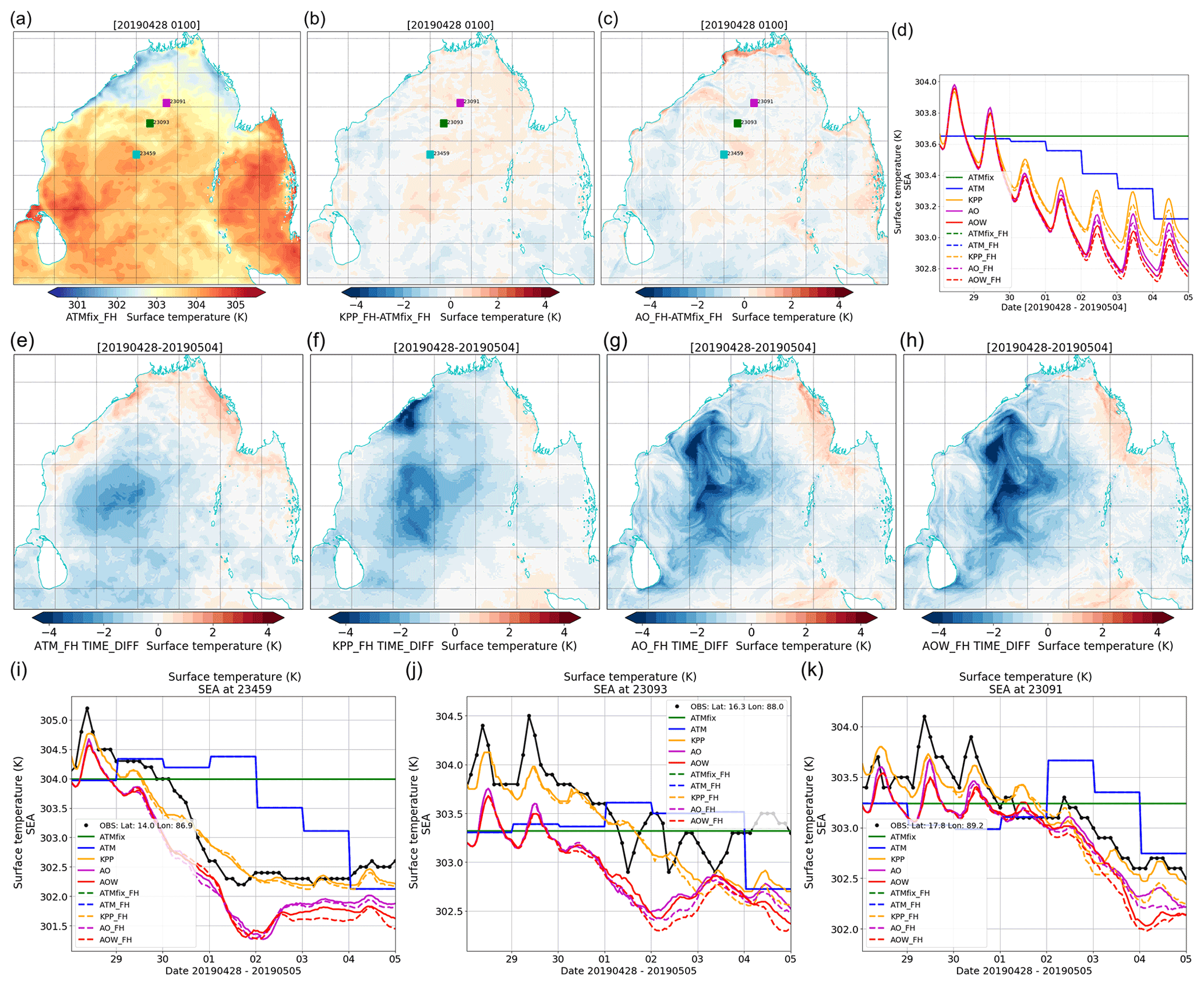
Figure 4 (a) Constant SST field in ATMfix(_FH) control simulation, based on OSTIA data available for forecasting at 00:00 UTC on 28 April 2019 for simulations of cyclone Fani (note central scale value of 303 K is approximately 30 ^∘C), and (b, c) initial-condition difference in SST for (b) KPP and (c) AO (and AOW) simulations. Note that ATMfix and ATM use same SST on the first day of simulations, and that initial conditions are common to each experiment with/without frictional heating. (d) Time series of regional mean SST for each experiment during the 7 d Fani case study, for the sub-domain shown in (a). (e–h) Difference in SST for ATM_FH, KPP_FH, AO_FH and AOW_FH simulations respectively at run final time compared to run start time, illustrating extent and magnitude of cyclone-induced cooling captured in each simulation. (i, j, k) Comparison of time series of SST from each experiment with in situ ocean buoy observations at 23459, 23093 and 23091 respectively (locations shown in Fig. 1 and panel a–c). Model data are taken as means in 5×5 grid neighbourhood surrounding each buoy location. Simulations without frictional heating are shown as solid lines, with frictional heating with dashed lines.

One of the limitations of the current experimental design of RCS-IND1 is that a free-running ocean-only simulation has been used to spin up the small-scale dynamics in the 3D ocean model component used in AO and AOW coupled runs. For the Titli case, the ocean initialization (Fig. 3c) is on average 0.6 K cooler than OSTIA, noting this is larger than the magnitude of mean observed cyclone-induced cooling during the event. Figure 3c shows this cooling is broadly distributed across the Bay of Bengal, though as much as 2 K cooler towards the eastern side. The KPP simulation for Titli is initialized on average about 0.2 K cooler than OSTIA, but with more varied spatial distribution of initial-condition differences. The mean initial condition for the Fani case is much more similar between all experiments, albeit with KPP initialization slightly warmer than OSTIA in the central and northern Bay of Bengal. When interpreting differences in the atmospheric response between experiments, it should be noted that not all experiments could be initialized from a common initial SST. Note also that while the SST imposed on the atmosphere in ATMfix and ATM are an observation-based foundation SST, representative of order 10 m below the ocean surface, the coupled system involves exchanging the top ocean model level temperature, typically within 1 m of the surface (e.g. Mahmood et al., 2021).

The diurnal cycle heating effect on SST evolution can be seen in Figs. 3d and 4d, with AOW ocean temperatures around 0.4 K warmer during the day than at night in periods when the influence of cyclones was less prevalent, such as after the passage of Titli (e.g. 14 October) and before the passage of Fani (e.g. 28 April 2019). Wave coupling leads to slightly reduced magnitude of diurnal warming than in AO for both cases, consistent with wave-enhanced mixing in AOW.

The magnitude and spatial distribution of cyclone-induced cooling is shown in Figs. 3e–h and 4e–h. Based on OSTIA data, Titli led to a decrease of 0.6 K in foundation SST, spread relatively evenly across the northern Bay of Bengal with the largest cooling over the whole period of 2.4 K. For KPP_FH, the maximum temperature decrease is 3.0 K, although the imprint of the passage of Titli can be more clearly seen in Fig. 3f than the OSTIA-based observations in ATM_FH (Fig. 3d). Larger but more focussed cooling of up to 3.8 K (AO_FH; Fig. 3g) and 4.3 K (AOW_FH; Fig. 3h) is evident when coupling to a 3D NEMO ocean component. Similar features can be seen for the Fani case. Figure 4d demonstrates that the OSTIA data available on 4 May 2019 (representative of satellite-observed ocean temperatures on 2 May 2019), on average 0.5 K cooler than on 28 April, do not yet represent the full extent of cyclone-induced cooling across the region. The largest OSTIA temperature reduction in the central Bay of Bengal during the period is 2.5 K (ATM; Fig. 4e), in contrast to more focussed and stronger cooling in coupled simulations of up to 4.8 K (KPP_FH; Fig. 4f), 5.9 K (AO; Fig. 4g) and 6.5 K (AOW; Fig. 4h). The more intense cyclone-induced cooling in AO and AOW than in KPP is consistent with the absence of upwelling using a 1D approach (Yablonsky and Ginis, 2009).

The different approaches to representing SST are compared to in situ ocean buoy data from three illustrative sites located in the central Bay of Bengal (see Fig. 1) in Figs. 3i–k and 4i–k. This analysis is complicated by the different ocean initialization approaches required across experiments, positional differences in cyclone track and intensity evolution, along with relatively infrequent and coarse numerical precision of reported ocean observations. There are also discrepancies between ocean buoys sampling within an order of 1 m of the surface, NEMO ocean temperatures representing the upper ocean model layer, and OSTIA representing a foundation SST. However, it is evident that AO and AOW simulations capture the scale of ocean cooling relatively well for the Titli case, though with cooling tending to initiate up to a day earlier than observed. Accounting for the KPP simulations being slightly warmer than observed at initialization, the magnitude of cooling is stronger than observed during Titli at buoy locations 23093 and 23091, but with KPP temperatures remaining too warm throughout the simulation at 23459 further south. It would be interesting to explore the sensitivity of Bay of Bengal SST to the representation of lateral advection, for example by running the NEMO ocean component without tides (e.g. Arnold et al., 2021), to better understand their influence on the KPP results.

For the Fani case, given that the initial-condition OSTIA data are up to 0.5 K cooler than buoy observations, the constant (ATMfix) and daily updating (ATM) SST assumptions in fact provide a reasonable 7 d approximation to observed temperatures in the northern Bay of Bengal (e.g. 7 d mean bias of −0.22 K at 23093 and 0.03 K at 23091 for ATMfix SST, relative to −0.70 and −0.33 K for AOW_FH at those buoys). The KPP runs are initialized with SST in good agreement with the observed buoys and provide a good representation of both the diurnal cycle ahead of Fani passing and of the observed cyclone-induced cooling later during the period at all three buoy locations. This leads to smallest root mean squared errors of all experiments for the KPP run (i.e. without frictional heating) of 0.25, 0.34 and 0.18 K at buoys 23459, 23093 and 23091 respectively. Initial-condition errors for AO and AOW are preserved through the simulations relative to observed SST, and there is some evidence that AO and AOW cool too much as the cyclone passes (e.g. 00:00 UTC on 2 May at 23459 and 00:00 UTC on 4 May at 23091). If removing initial-condition offsets, however (not shown), AO has the smallest mean bias and root mean squared errors (RMSEs) of all experiments relative to observations for buoy location 23091 (RMSE of 0.16 K) and 23093 (RMSE of 0.23 K), whereas KPP has slightly lower RMSE at 23459 (RMSE of 0.44 K).

The SST time series in Figs. 3 and 4 also highlight some sensitivity in KPP, AO and AOW simulations to the representation of frictional heating in the coupled atmosphere component. Small differences in SST evolve after about 3 (Titli) or 4 (Fani) days between equivalent simulations with or without frictional heating, with the introduction of frictional heating leading to stronger induced ocean cooling (due to more intense storm development), and SST of order 0.2 K cooler than for runs without this process enabled. The fit relative to observed SST, after removing initial-condition offsets, is similar but slightly degraded in coupled simulations using frictional heating for the locations plotted in Figs. 3 and 4. It can also be concluded that the influence of frictional heating is of secondary importance relative to the choice of coupling approach for SST evolution over the 7 d period for both cases.

3.3 Tropical cyclone structure, track and intensity

Cyclone tracks have been diagnosed from mean sea level pressure (MSLP) and relative vorticity at 850 hPa (850RV) model diagnostics for each experiment conducted using the method described by Heming (2017). Storms are initially identified based on a search for the highest 850RV within a 3^∘ radius of an observed cyclone centre position, followed by a search for minimum MSLP within 3^∘ radius of that point. For a storm to be diagnosed from model outputs, the maximum 850RV must be above $\mathrm{4}\times {\mathrm{10}}^{-\mathrm{4}}$ s⁻¹ and minimum MSLP below 1010 hPa, with both thresholds and the search radii being tuneable.

Simulated maximum wind speed and diagnosed tracks for the Titli case are compared in Fig. 5 (for experiments with frictional heating), alongside an illustration of the observed cyclone structure as it neared landfall from Meteosat satellite imagery at 00:00 UTC on 10 October 2018 and a multi-agency observed track as diagnosed and shared via the Global Telecommunication System (GTS) in near-real time during each event, based on bulletins from Regional Specialized Met Centres (RSMCs), tropical cyclone warning centres, and the Joint Typhoon Warning Center (Heming, 2017). Contours of outgoing longwave radiation at the equivalent time are plotted to illustrate the simulated cyclone structure. Corresponding results for simulations without frictional heating are provided for reference in Supplement Fig. S1. Results for Cyclone Fani are presented in Fig. 6 (see also Supplement Fig. S2), where the observed cyclone structure is shown by brightness temperatures from the INSAT satellite at 06:00 UTC on 2 May 2019. Results from both cases provide qualitative evidence that the RCS-IND1 configuration can be used to simulate intense storm development over the Bay of Bengal with realistic cloud structures and peak simulated winds aligning with the diagnosed model track that are generally well aligned to observed tracks.

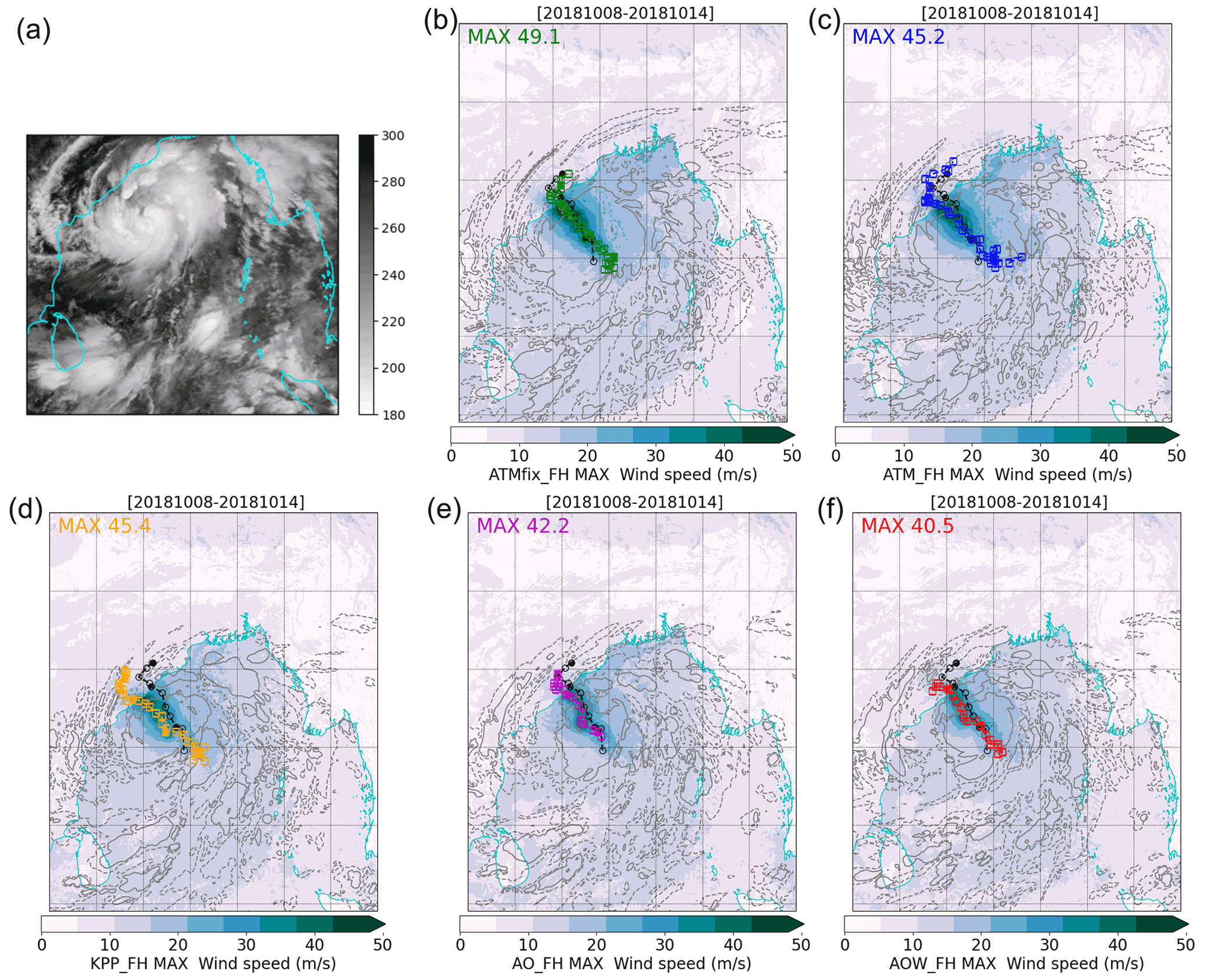
Figure 5 (a) Illustration of Cyclone Titli satellite-observed brightness temperature from Meteosat at 00:00 UTC on 10 October 2018. In (b)–(f), results from RCS-IND1 experiments showing maximum wind speed during the 7 d simulation (coloured shading). Also plotted is the diagnosed simulated cyclone track at 3-hourly intervals (coloured line and squares) compared with observed track at 6-hourly intervals (black line and circles). Line contours show instantaneous simulated outgoing longwave radiation at top of atmosphere (dashed line indicating 150 W m⁻², solid line 100 W m⁻² contour) at coincident hour to the satellite observation in (a). See Fig. S1 in the Supplement for corresponding figure for simulations without frictional heating enabled.

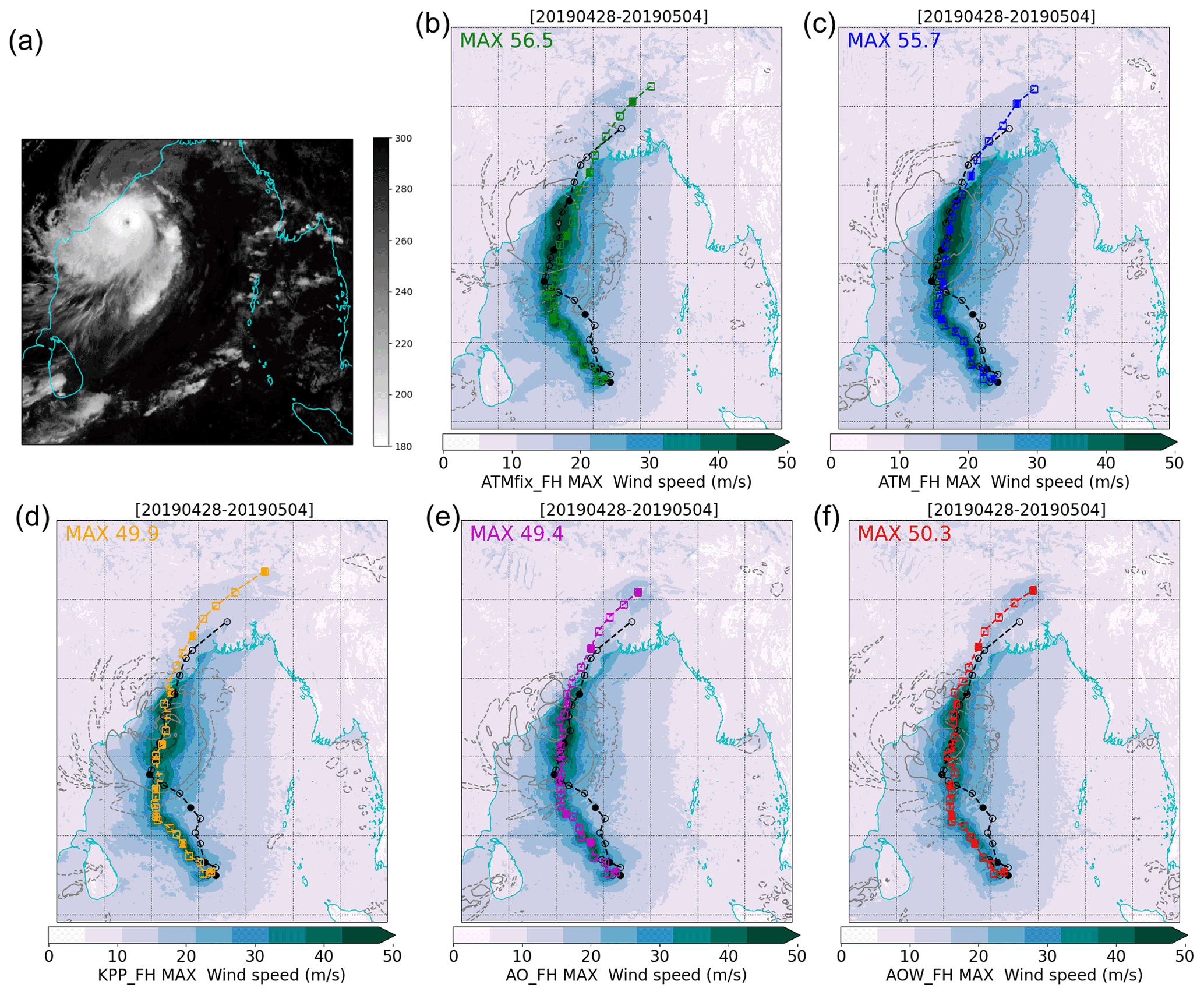
Figure 6 (a) Illustration of Cyclone Fani satellite-observed brightness temperature from INSAT at 06:00 UTC on 2 May 2019. In (b)–(f), results from RCS-IND1 experiments showing maximum wind speed during the 7 d simulation (coloured shading). Also plotted is the diagnosed simulated cyclone track at 6-hourly intervals (coloured line and squares) compared with observed track at 6-hourly intervals (black line and circles). Line contours show instantaneous simulated outgoing longwave radiation at top of atmosphere (dashed line indicating 150 W m⁻², solid line 100 W m⁻² contour) at coincident hour to the satellite observation in (a). See Fig. S2 for corresponding figure for simulations without frictional heating enabled.

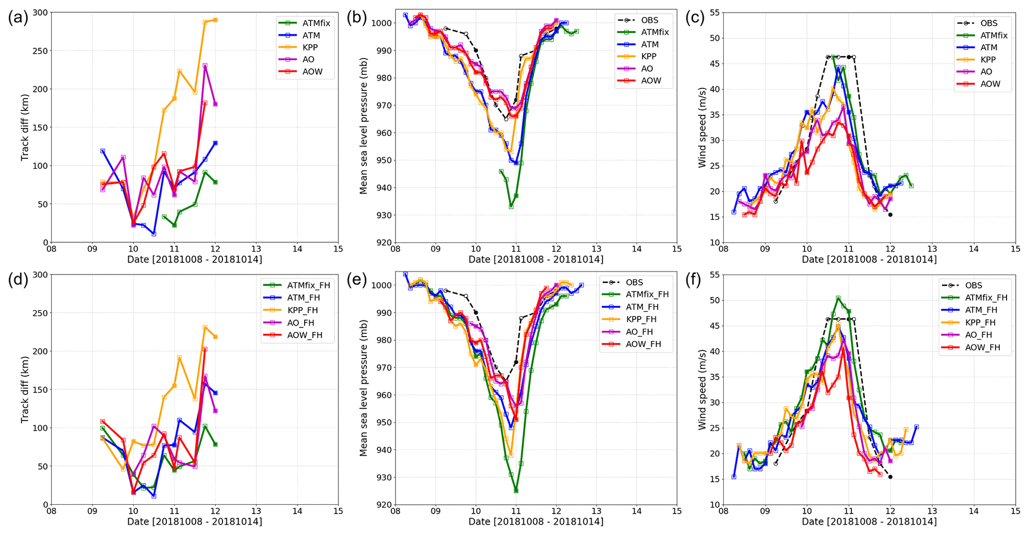
Figure 7 Comparison of observed and simulated cyclone track statistics for all simulations of cyclone Titli. Panels (a)–(c) show results without and (d)–(f) with frictional heating represented. Panels (a) and (d) show difference between coincident simulated and observed track position, (b) and (e) show mean sea level pressure at diagnosed track centre, and (c) and (f) show along-track maximum wind speed. Observed track data are taken from the SXXT50 bulletin based on satellite data interpretation.

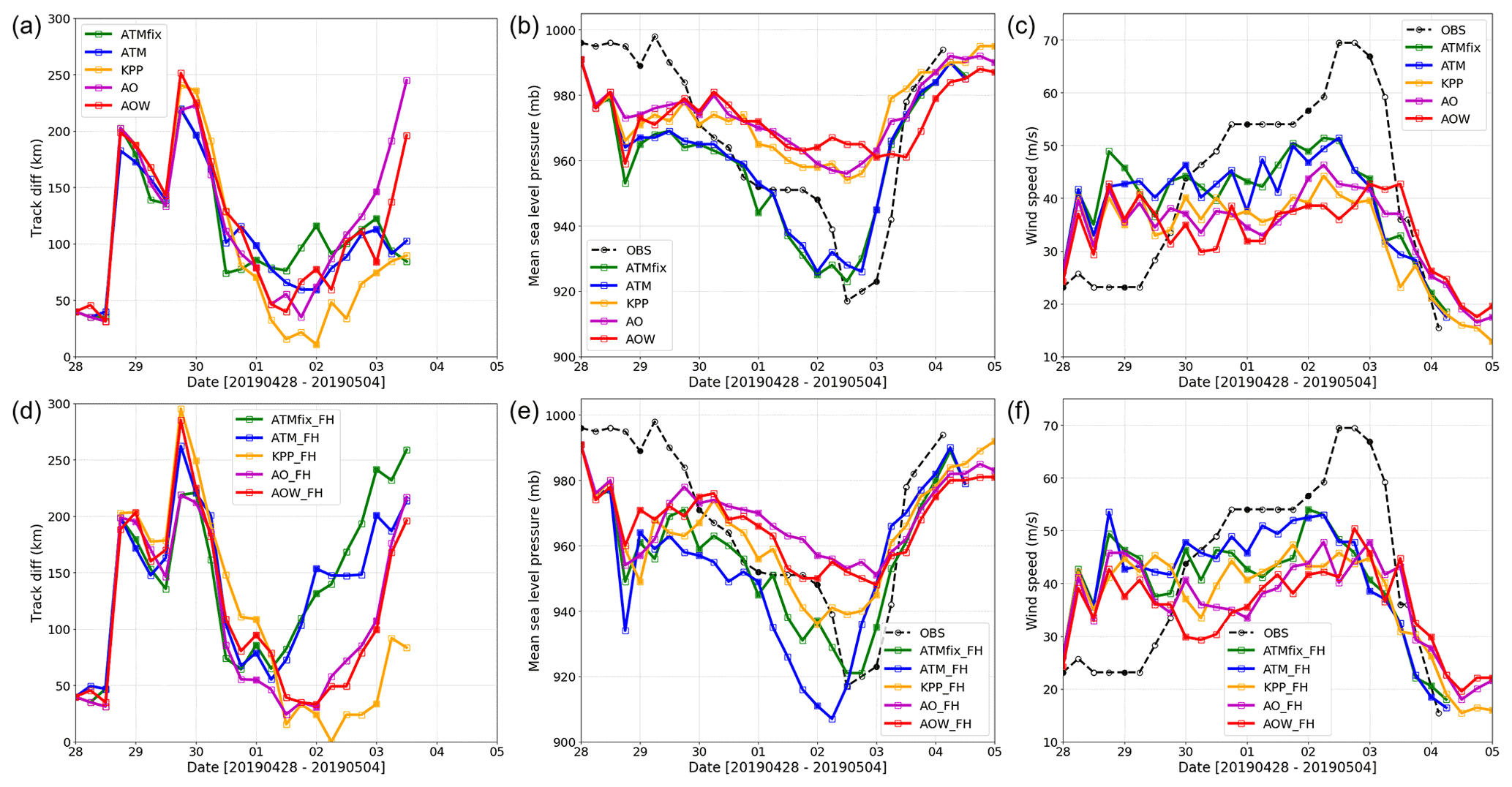
Figure 8 Comparison of observed and simulated cyclone track statistics for all simulations of cyclone Fani. Panels (a)–(c) show results without and (d)–(f) with frictional heating represented. Panels (a) and (d) show difference between coincident simulated and observed track position, (b) and (e) show mean sea level pressure at diagnosed track centre, and (c) and (f) show along-track maximum wind speed. Observed track data are taken from the SXXT50 bulletin based on satellite data interpretation.

Figures 7 and 8 provide a more quantitative comparison of the diagnosed track and intensity for all experiments considered for the Titli and Fani cases respectively. Summary metrics are provided in Table 8. An important result from Figs. 7 and 8 is evidence that while coupling tends to drive the same differences between experiments whether run with or without frictional heating, including the frictional heating contribution to the boundary layer energy budget can have as large an impact on cyclone characteristics as the introduction of model coupling. The relative impact of coupling on results with and without frictional heating is therefore considered within the same discussion below.

Table 8 Summary of observed and simulated cyclone statistics for Titli and Fani cases. Figures in round bracket italics indicate results from simulations with frictional heating enabled, with differences listed in square brackets. Underlined values indicate which of the simulations with or without frictional heating give the closest metric to observed data for a given run type. Bold values indicate which simulation has the best metric across all experiments conducted. The final row summarizes difference between highest and smallest simulated values. ^* ATMfix cyclone tracking identified the cyclone later than for other experiments.

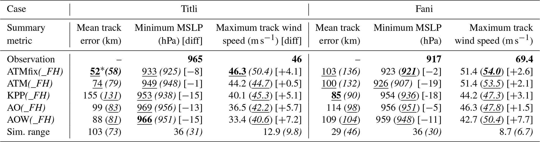
While Fani was considerably longer lived and more intense than Titli, the sensitivity of cyclone intensity to coupling is similar for both cases. The lack of air–sea interaction in ATMfix (ATMfix_ FH) results in deeper cyclones, by 33 hPa (31 hPa) for Titli and 36 hPa (30 hPa) for Fani, compared to the fully coupled AOW (AOW_FH) simulations. This is consistent with the well-established result that the representation of surface cooling feedbacks in coupled simulations tends to limit cyclone intensification (e.g. Vincent et al., 2012; Feng et al., 2019; Vellinga et al., 2020; Saxby et al., 2021). This demonstrates considerable sensitivity to ocean state for both cases, and greater than typically found in other studies. For example, Vellinga et al. (2020), based on assessment of global coupled UM forecasts, showed differences of the order of 10 hPa between central pressure in coupled and uncoupled simulations across different ocean basins by 168 h into a forecast, although with extreme cases having differences of order 20 hPa. Rai et al. (2019) showed that use of a relatively cooler (0.2–0.4 K cooler than control) time-evolving SST data product could lead to about 7 hPa more intense storms after 78 h forecast time over the Bay of Bengal in atmosphere-only experiments. It should be noted, however, that SST differences between ATMfix and AOW of up to 2 K develop in the RCS-IND1 simulations, initialized around 3–4 d ahead of the deepest cyclone intensity, and based on different initial ocean states.

3.3.1 Cyclone Titli

For Titli, the ATMfix and ATM uncoupled and KPP coupled simulations are found to over-deepen relative to the observed intensification, while the AO and AOW coupled results with a 3D ocean model component are considerably closer to the observed minimum pressure. This conclusion is common to simulations with and without frictional heating. The over-deepening is consistent with relatively warmer initial-condition SST in the KPP and uncoupled simulations in the cyclone genesis region (Fig. 3b, i), and the simulated cyclone being too intense may have contributed to the excessive cooling of KPP in the northern Bay of Bengal relative to observations (Fig. 3k). All cyclone simulations deepen more quickly than observed, although AO and AOW intensify later than the uncoupled and KPP simulations for this case. The addition of wave coupling in AOW results in slightly earlier intensification than AO, particularly with frictional heating (Fig. 7e). This may reflect the different paths that AO and AOW storms take around 10 October (Fig. 7d), with AO_FH tracking relatively westward of the observed track earlier than AOW_FH (Fig. 5e and f).

The smallest cyclone track errors are evident for the ATMfix(_FH) experiments (Fig. 7a, d), with tracks deviating westward in ATM(_FH) and all coupled experiments. This westward trajectory is particularly pronounced for the KPP(_FH) coupled simulations (Fig. 5d). Katsube and Inatsu (2016) illustrated a tendency for TCs in the north-west Pacific to recurve faster over relatively warmer oceans for storms in the north-west Pacific and thereby propagate relatively rightward of a simulation with intermediate SSTs. Over relatively cooler oceans, they found slower re-curvature and leftward propagation. The RCS framework provides the capability to perform such sensitivity experiments for these cases, and it would be of interest to examine if similar processes account for track deviation in the Bay of Bengal, although beyond the scope of the current study. Rather, it can at least be noted that the relatively westward propagation is consistent with more slowly intensifying cyclones in coupled cases over a relatively cooler ocean. The reasons for KPP deviating so far to the west for the Titli case, further westward than AO and AOW, resulting in largest track errors, are, however, unclear. For KPP, AO and AOW, the track trajectory is improved with representation of frictional heating (i.e. westward tendency reduced), consistent with relatively quicker storm intensification and deeper storms developing.

3.3.2 Cyclone Fani

By contrast, the coupled simulations for Fani, which deepened considerably to an observed minimum MSLP of 917 hPa, are considerably too weak (minimum simulated central pressure in AOW of 959 hPa), and unlike for Titli, the KPP results are now more similar to the AO and AOW coupled simulations. It is notable that none of the simulations captured the initial northward propagation and relative delay to intensification of Fani's evolution, with all simulated storms deepening within the first day of simulation and thereby veering westward too early. This suggests errors in the common initial conditions inherited from the global model analysis. Further analysis (not shown) indicated that the initial stages of the Fani simulations may have been degraded by distortion of the cyclonic vortex within the global operational analysis used in the initialization, suggesting that RCS-IND1 results may improve with implementing a vortex initialization scheme for experiments specially aimed at simulating tropical cyclones (e.g. Liu et al., 2020).

All simulated storms turned northward from around 3 d into the simulation, when the uncoupled simulations further deepened and track errors were much reduced (Fig. 8a, d). Over-deepening over a relatively warm ocean SST is associated with a rightward-propagating cyclone for ATMfix(_FH) and ATM(_FH), such that ATMfix(_FH) tracks to the east of the observed track. This is more pronounced when frictional heating is applied (ATMfix_ FH). In contrast, each of coupled simulations KPP(_FH), AO(_FH) and AOW(_FH) track along the observed path from 30 April 2019, with AOW(_FH) having slightly improved track relative to AO(_FH). After landfall early on 3 May 2019, the diagnosed tracks in coupled simulations progress too far north, consistent with relatively slower deintensification. Track errors are reduced when frictional heating is included in all coupled simulations, consistent with more intense storms developing.

3.3.3 Summary impact of frictional heating

The approach of not including the heating term in uncoupled regional UM configurations to date as a pragmatic means to improving model results seems to be supported in results for both Titli and Fani cases, with ATMfix_FH and ATM_FH over-deepening and thereby having larger errors of MSLP and track position relative to the equivalent ATMfix and ATM simulations without frictional heating. Track errors are more impacted for Fani than Titli, for which ATM_FH considerably over-deepens from 1 May to a minimum central MSLP as low as 907 hPa. In contrast, addition of frictional heating improves track errors for AO and AOW coupled simulations for both Titli and Fani, and there seems to be some improvement to the timing of the dissipation phase. While more intense storms are simulated for Fani with AO_FH and AOW_FH than for the equivalent runs without frictional heating, its impact is insufficient to deepen as much as observed or uncoupled simulations. There is also some indication that the relative impact of coupling on simulations may be slightly reduced with frictional heating (i.e. range of pressure and wind speeds smaller between experiments). These results lead to the recommendation that while it continues to be pragmatic to disable frictional heating when running the UM in uncoupled modes, coupled results can be improved when frictional heating is active. In summary, by representing coupled feedbacks it appears possible and desirable to include an additional term in the energy budget of regional simulations and thereby provide a fuller representation of the physics of tropical systems.

3.4 Impact of coupling on wind speed

In general, the comparison of track-diagnosed wind speed relative to those indicated in the real-time GTS bulletins in Figs. 7 and 8 show that all simulations under-predicted peak wind speeds, particularly for the Fani case. Saxby et al. (2021; see their Fig. 5) illustrated from their analysis of a larger number of simulated TC cases in the Bay of Bengal and a range of initialization times that the wind–pressure relationship for kilometre-scale UM simulations has generally overly low winds for given MSLP relative to observations above around 35 m s⁻¹, with those errors being reduced but not eliminated with coupling. This is consistent with the parameterization of surface drag in RAL1-T (see below). The over-deepening of uncoupled simulations for both cases shown here therefore gives closer agreement to the observation-based peak wind, while frictional heating also leads to deeper and thereby stronger winds. With frictional heating, the UM can generate intense storms with insufficient maximum wind speeds (i.e. deepest MSLP of 907 hPa with maximum wind speed 54 m s⁻¹ for ATM_FH in Table 8), while in the equivalent coupled simulations, cyclones do not deepen sufficiently albeit with relatively stronger wind speeds for given MSLP (e.g. AOW_FH deepened to 948 hPa with maximum wind speed 50.4 m s⁻¹).

These results are supported by a comparison of simulated wind speed at 10 m above the surface with in situ observations near landfall on the Indian coast (Gopalpur; Fig. 1) and at two ocean buoy locations in the Bay of Bengal, shown for Titli and Fani cases in Fig. 9. As discussed in Sect. 3.2, quantitative comparison with observations is challenging due to the different cyclone tracks in each simulation, and potentially substantial observation errors both during extreme conditions and above the ocean. Some caution might therefore be applied to the apparent tendency for simulations to have stronger wind speeds than observed by ocean buoys during both cases, although is it clear that stronger winds are simulated with fixed and daily updating SST than for any of the coupled simulations, which tend to have improved bias and RMSE statistics. AO_FH and AOW_FH have statistically significant improvements to the bias relative to ATMfix_FH at 95 % confidence level for both 23091 and 23093 buoy locations shown for both Titli and Fani cases. Note similar statistically significant bias improvement is also found for KPP_FH for both cases at 23091, but only for Titli at buoy 23093 (i.e. KPP_FH wind speed bias at 23093 is statistically indistinguishable from ATMfix_FH results for Fani at 95 % level). The overly rapid deintensification of Titli in uncoupled simulations is also evident in comparison with observations at 23091 (Fig. 9c), where the beneficial impact of frictional heating can be seen by the final simulation day.

Figure 9 Comparison of observed (black lines) and simulated wind speed at (a, d) Gopalpur coastal location, (b, e) 23093 ocean buoy and (c, f) 23091 ocean buoy during (a–c) Titli, and (d–f) Fani case study periods. See Fig. 1 for summary of observation locations. Note that different y-axis scales are used in each panel. Simulation results without (solid lines) and with frictional heating (dashed lines) are provided, based on mean of 5×5 neighbourhood of grid points nearest the observation point.

Consistent with along-track results for Titli (Fig. 7c, d), comparisons at Gopalpur (Fig. 9a) show that only peak simulated wind speed with ATMfix of 21 m s⁻¹ starts to approach the observed maximum wind speed of around 30 m s⁻¹. The timing of maximum wind speeds matches observations well, however. AO_FH provides the best match to observed peak winds at Gopalpur for the Fani case (Fig. 9d), although the timing is slightly delayed relative to observations. These results also clearly show peak winds too early in uncoupled simulations relative to observations, noting that peak wind speeds from the uncoupled simulations are relatively weaker at this location given that the simulated storm tracked further eastward than observed (Fig. 6b, c). The impact of wave coupling on wind speeds is relatively small during both cases. Some improvements to the earlier timing and greater magnitude of maximum winds with frictional heating is evident for KPP_FH, AO_FH and AOW_FH simulations relative to equivalent runs without frictional heating. This is consistent with the relative additional surface heating generating stronger, more rapidly developing storms. However, in comparison with the clear impact on cyclone track and intensity, the sensitivity of cyclone winds away from the cyclone track to frictional heating is relatively small for these cases.

Developments to improve the wind speed characteristics of the RCS-IND1 configuration are in progress, and their impact will need to be evaluated in future studies. A key consideration is the representation of surface drag at high wind speeds (more than 30 m s⁻¹). Different approaches to change the UM drag parameterization under investigation were discussed recently by Gentile et al. (2021) in the context of kilometre-scale coupled UM simulations of extratropical cyclones. This includes testing the impact of moving to the COARE 4.0 parameterization at lower wind speeds, with a cap and reduction in drag coefficient at higher wind speeds. In the RAL1 physics configuration used in the current study, the drag coefficient is assumed to increase linearly as a function of wind speed, implying that winds are excessively dampened at higher wind speeds, consistent with the increasing wind speed bias with deeper MSLP introduced above. This is known to be unrealistic, with Donelan (2018) for example arguing that a reduction in the drag coefficient above 30 m s⁻¹ was critical to representing rapid intensification. It will therefore be important to re-examine these and other cyclone cases using revised RAL physics definitions. For example, Baki et al. (2022) found simulation of TCs in the Bay of Bengal could be improved by up to 16 % for wind speed using optimal parameters of the WRF model based on sensitivity analysis of a range of physics parameters.

3.5 Impact of coupling on precipitation

The impact of coupling on accumulated precipitation is illustrated for Titli and Fani cases in Figs. 10 and 11 respectively, and a more quantitative comparison of the domain-accumulated precipitation is shown in Figs. 12 and 13. Results are compared with the NASA GPM (Global Precipitation Measurement; Hou et al., 2014) IMERG observations, with all precipitation data interpolated to the GPM resolution of 0.1^∘ prior to analysis and expressed as the cumulative precipitation depth over the defined area for a given period of interest. The influence of model spin-up from global-scale atmosphere initialization can be seen during the first day of each simulation (Figs. 12a, d and 13a, d) and thereby the first day is omitted from the following analysis. Figures 10 and 11 demonstrate relatively good simulation of the spatial extent of precipitation across the Bay of Bengal associated with both cyclones and their subsequent eastward passage following landfall. All simulations tend to have too little light precipitation, which is a common feature of convective-scale UM simulations with RAL1-T configuration (Bush et al., 2020). This is illustrated by relatively fewer accumulations of less than 100 mm in all simulations than observed by GPM in Figs. 12c, f and 13c, f. There is, however, better agreement with GPM for the relative frequency of higher accumulated precipitation totals.

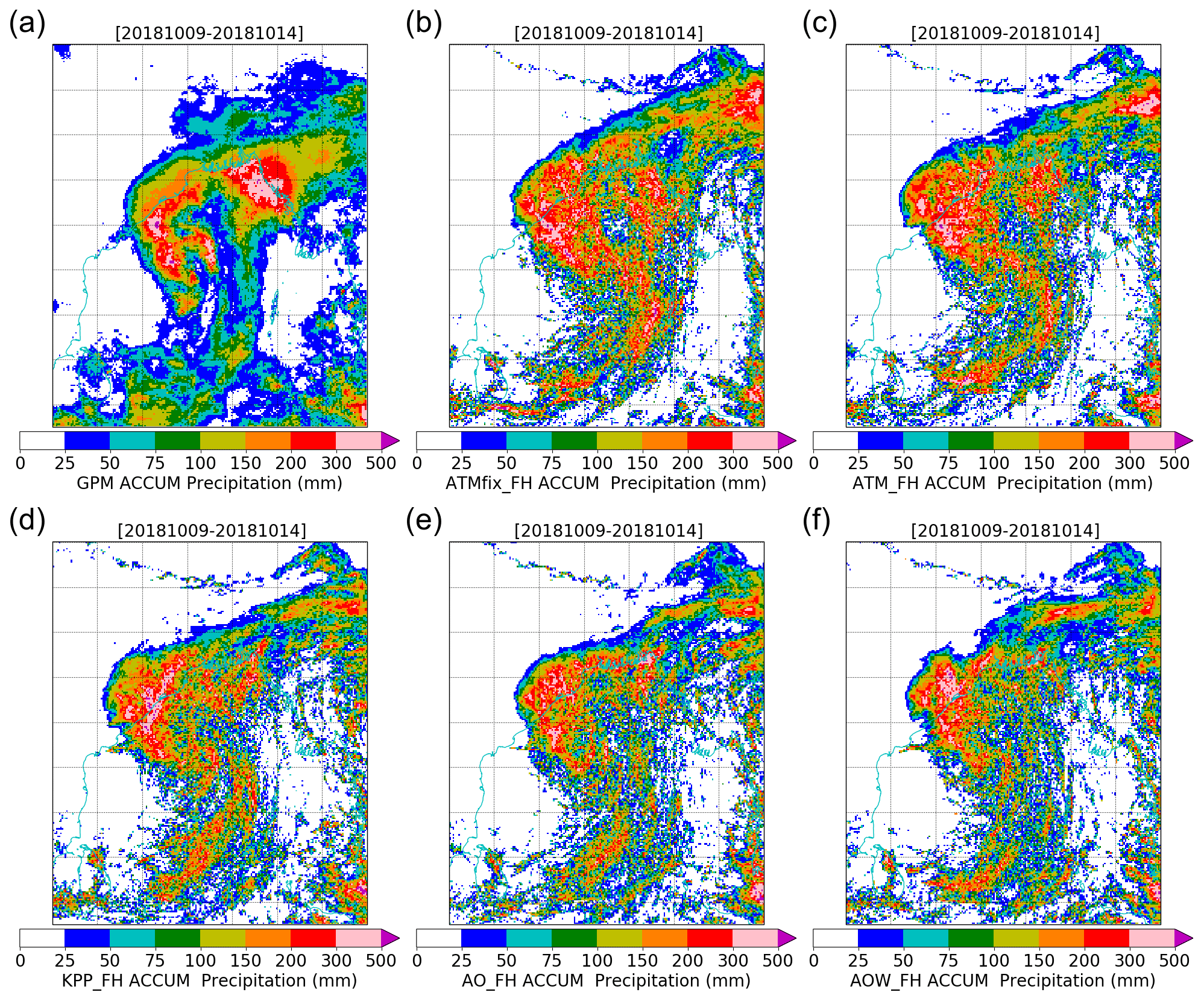
Figure 10 7 d precipitation accumulation during Titli case study over Bay of Bengal sub-domain region (a) observed by GPM (NASA Global Precipitation Measurement) and simulated by (b) ATMfix_FH, (c) ATM_FH, (d) KPP_FH, (e) AO_FH and (f) AOW_FH. All simulated data are interpolated to the GPM resolution prior to computing accumulations. See Fig. S3 for corresponding figure for simulations without frictional heating enabled.

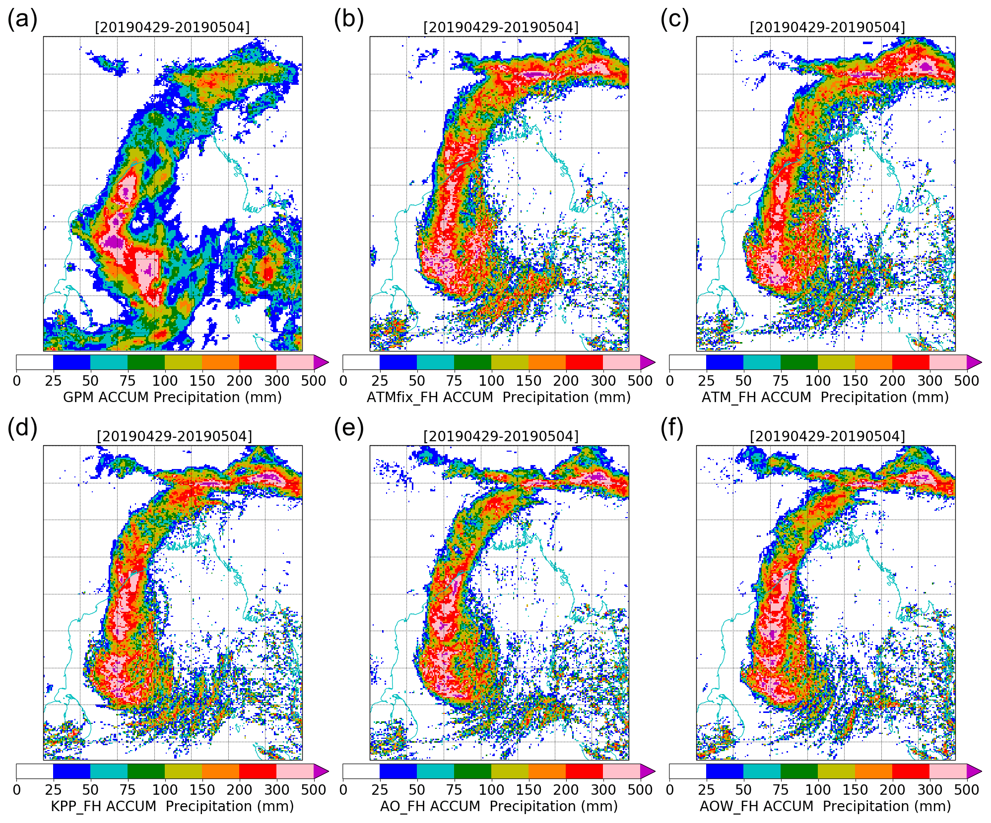
Figure 11 7 d precipitation accumulation during Fani case study over Bay of Bengal sub-domain region (a) observed by GPM (NASA Global Precipitation Measurement) and simulated by (b) ATMfix_FH, (c) ATM_FH, (d) KPP_FH, (e) AO_FH and (f) AOW_FH. All simulated data are interpolated to the GPM resolution prior to computing accumulations. See Fig. S4 for corresponding figure for simulations without frictional heating enabled.

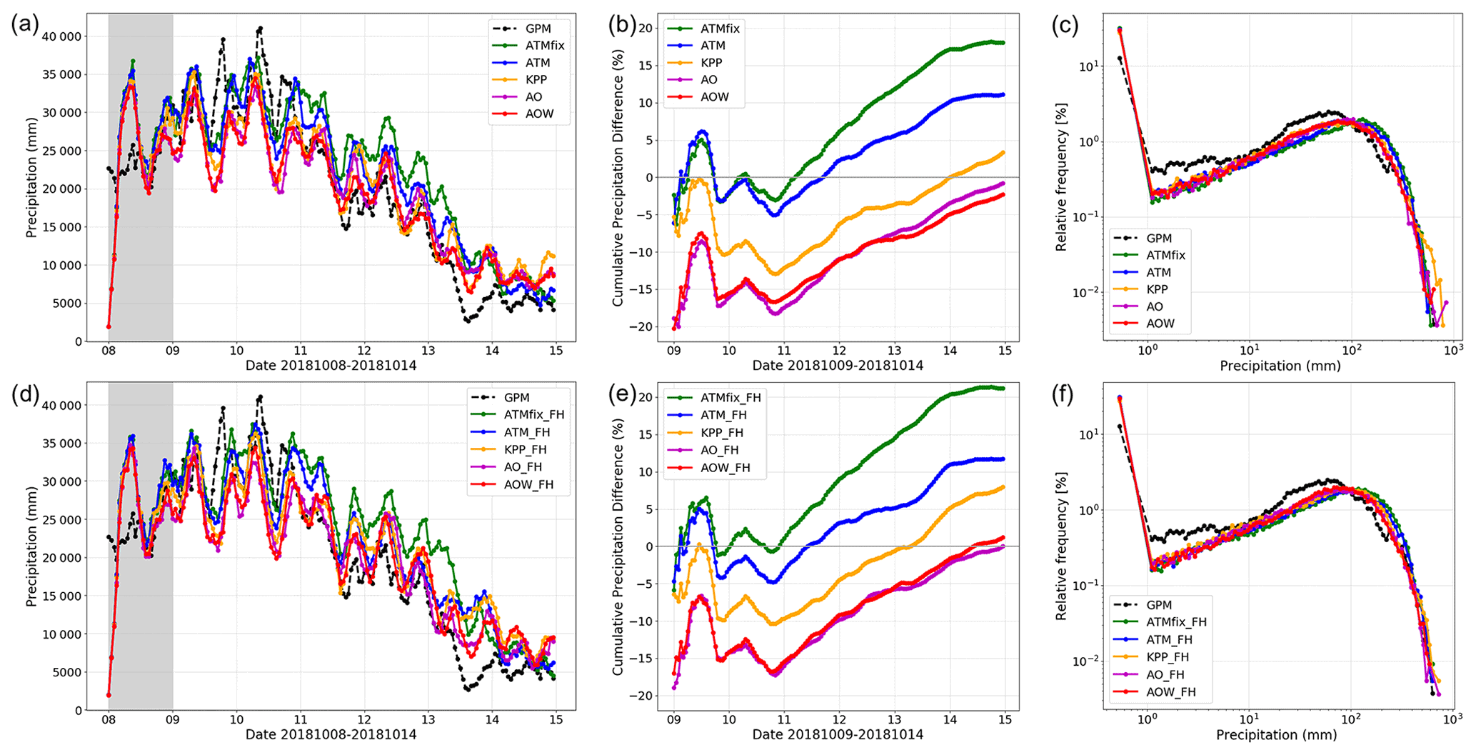
Figure 12 Comparison of Bay of Bengal sub-domain precipitation characteristics for Titli case study for simulations (a–c) without and (d–f) with frictional heating enabled. (a, d) Time series of sub-domain accumulated precipitation for region shown in Fig. 10. (b, e) Cumulative percentage difference between simulated precipitation and GPM observations, computed after day 1 of simulation to avoid spin-up effects. (c, f) Frequency distribution of 7 d accumulated precipitation relative to GPM.

The over-intensification of uncoupled simulations of Titli is evident in Fig. 12 with ATMfix(_FH) accumulated precipitation consistently higher than observed after 11 October, contributing to a net over-prediction of accumulated precipitation of 18 % (21 %) for ATMfix (ATMfix_FH) and 11 % (12 %) for both ATM (ATM_FH) simulations. Coupled simulations have a net deficit of accumulated precipitation during the first half of the Titli case study relative to GPM, but over the 6 d period KPP has slightly higher accumulated precipitation (3 % higher than GPM for KPP and 8 % for KPP_FH) while AO(_FH) and AOW(_FH) are well matched (biases of AO: −1 %, AO_FH: 0 %; AOW: −2 %; AOW_FH: 1 %). For the Fani case (Fig. 13), all simulations miss the peak in observed precipitation on 30 April 2019, perhaps associated with the lack of initial northward cyclone propagation. ATMfix and ATM simulations then have relatively good estimates of Bay of Bengal regional accumulation (6 d accumulation bias of 1.5 % and 0.5 % respectively), but with higher accumulations when frictional heating was applied, consistent with a more intense simulated cyclone (biases of 6 % for ATMfix_FH and 2 % for ATM_FH). For this case, the KPP, AO and AOW results tend to underpredict accumulated precipitation (by 9 % for KPP and 12 % for AO and AOW), particularly after landfall early on 3 May 2019, with enhanced precipitation and a slightly improved agreement relative to GPM with frictional heating (bias of −6 % for KPP_FH and −10 % for both AO_FH and AOW_FH).

Figure 13 Comparison of Bay of Bengal sub-domain precipitation characteristics for Fani case study for simulations (a–c) without and (d–f) with frictional heating enabled. (a, d) Time series of sub-domain accumulated precipitation for region shown in Fig. 10. (b, e) Cumulative percentage difference between simulated precipitation and GPM observations, computed after day 1 of simulation to avoid spin-up effects. (c, f) Frequency distribution of 7 d accumulated precipitation relative to GPM.

In common with the wind speed results, it will be valuable to re-examine the impact of using revised RAL configurations on the RCS-IND1 precipitation characteristics. For example, development of a new bimodal diagnostic cloud fraction (Van Weverberg et al., 2021) and cloud microphysics (e.g. Hill et al., 2015) parameterizations in RAL offer pathways towards improving the frequency distribution of simulated precipitation. Improving the representation of precipitation in RCS-IND1 is a key priority in the context of coupled prediction given the opportunity to further assess and develop the land surface model component to enable a more integrated approach to simulating the terrestrial water cycle (e.g. Lewis and Dadson, 2021). This is of particular importance in the Bay of Bengal given potential feedbacks through the ocean state (e.g. Krishnamohan et al., 2019).

3.6 Computational resources

Table 9 provides a summary of the computational resources required to run different RCS-IND1 configurations of the RCS modelling framework. Simulations discussed in this paper were conducted on the Met Office Cray XC40. Reported values indicate that the RCS provides a suitable tool for running research configurations within a practical time limit, with configurations typically completing a day simulation within the order of a 20 min runtime. Run times for comparable simulations run on the NCMRWF Cray XC40 are also listed, with the RCS having been successfully ported to that machine to enable ongoing collaboration and motivate new simulation experiments. Considerable opportunities for system optimization are thought to exist in both the regional model components and coupling interfaces, which will be implemented in future updates. For example, updating the wave model component from WAVEWATCH III vn4.18 to vn7.2 is anticipated to enable coupling to be performed independently between each model processor, rather than coupling via a single processor as required at present.

Table 9 Summary of the typical computational resources required to run RCS-IND1 experiments, runtimes and output data volumes for completing a day simulation. Run durations quoted in row ¹ were completed using the Met Office Cray XC40, and those completed in row labelled ² were completed using the NCMRWF high-performance computing server Mihir Cray XC40. Two output data volume rows are given. The diagnostic output (row ³) shows output data size saved to disk for daily restart and model variables of interest to enable analysis. Note number and type of output diagnostics are dependent on user specifications, but values are indicative of default RCS-IND1 configurations and data volumes typically archived. The coupling output (row ⁴) shows the volume of data written to disk to support coupling exchanges (computed as difference between total output volume quoted in daily log file and the diagnostic output size on disk). Note that the data volumes required for coupling are less user specific, and these data are not relevant for archiving but will scale with choice of coupling frequency. All values reflect configurations without optimization.

4 Discussion and ongoing development

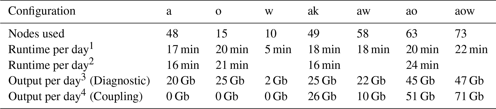
A new implementation of a flexible regional coupled modelling framework focussed on the Indian region has been described. The primary motivation for this development is to provide underpinning capability for research into the sensitivity of hazardous weather and its impacts to how interactions are represented within simulations of the environmental system. This research may ultimately lead to improved operational predictions and services delivered through the Indian Ministry of Earth Sciences. Given the high population density, particularly in coastal regions, and prevalence of natural hazards linked to the Indian monsoon progression, these research questions and operational impacts are of critical importance.

This paper documents the scientific and technical basis of the RCS-IND1 implementation, with aspects of its flexibility to support a range of experimental designs highlighted to motivate a breadth of future research activities using these capabilities. Results have been presented to demonstrate the sensitivity of simulations of cyclone Titli and Fani with a variety of approaches to the representation of the ocean, including uncoupled atmosphere simulations with fixed SST (ATMfix), daily updating OSTIA (ATM), a simplified coupled system with the ocean represented by a 1D mixed layer parameterization (KPP), and coupling to a 3D ocean model (AO) or coupling to both ocean and wave models with two-way interactions between all components (AOW).

The relative influence of frictional heating in the UM boundary layer formulation has also been examined. This study confirms that the uncoupled simulations still tend to be optimized without frictional heating. While the sensitivity to coupling is consistent with and without frictional heating, results show that coupling effectively enables this term to be included in a convective-scale simulation. Although Fani was a stronger storm than Titli, and the effect of frictional heating might be expected to be more significant for more intense storms, these results show a broadly similar difference between results with and without frictional heating for each case. A broader study of the sensitivity of coupled results to frictional heating, in particular to assess the sensitivity of runs with earlier initialization times would be of interest to assess its impact during initial cyclogenesis (e.g. Kilroy et al., 2017).

All simulations demonstrate some long-standing model biases that are not substantially corrected through model coupling, such as a tendency for winds to be too light for a given MSLP, and insufficient light rain. While the introduction of air–sea interactions through coupling markedly improves the intensification of Titli to be closer to observations, the reduced intensification leads to poorer simulation of minimum pressure but improved cyclone track prediction for Fani. These results are consistent with the analysis of Saxby et al. (2021), who provide a review of RCS-IND1 performance for ATM and AO configuration across a broader range of cyclone cases.

For the two TC cases discussed in this paper, coupling with the waves shows smaller impact than coupling with the ocean. This contrasts with the sensitivity found for extra-tropical cyclones (Gentile et al., 2021), potentially as the wave feedback on drag saturates for the higher wind speeds found in TCs. Work is ongoing to assess the representation of surface drag in both coupled and uncoupled configurations in RCS-IND1, noting that the RAL1-T science definition does not cap the drag at higher wind speeds, as employed in some parameterizations (see discussion in Sect. 3.4).

For these cases, a 1D mixed layer scheme shows similar first-order SST cooling and feedback on the atmosphere as for coupling to a full 3D ocean model. Nevertheless, the 3D ocean generally shows stronger localized cooling than the 1D mixed layer ocean. This is consistent with shear-induced mixing of the upper ocean being the main cooling mechanism, with 3D ocean upwelling playing a secondary role (Yablonsky and Ginis, 2009). As discussed by Singh et al. (2021) for the Fani case, effective incorporation of ocean initial conditions (surface and sub-surface) is vital for effective representation of cyclone genesis and intensification, and thereby improving these aspects in the RCS framework remains a priority.

Further scientific and technical development of the RCS-IND1 configuration is planned. Key research priorities include the following:

• analysis of ocean and wave performance of RCS-IND1, for example associated with the ocean response to cyclone evolution;

• improving the initialization of components, in particular the regional ocean, for example based on initialization from equivalent uncoupled regional analyses or through developing regional weakly coupled data assimilation;

• reviewing and improving the conservation of the surface momentum budget across the atmosphere–wave–ocean interface and its treatment between the three component models;

• understanding the sensitivity of air–sea interaction and optimizing results to the choice of coupling frequency;

• demonstrating and assessing application of RCS-IND1 for concurrent multi-hazard prediction, such as wind–tide–surge interactions and coastal flooding;

• understanding the impact of choice of lateral boundary conditions on system performance, for example to establish the sensitivity to use of coupled or uncoupled global model boundaries;

• assessment of the impact of convective-scale precipitation on the land surface, and thereby representation of the terrestrial water cycle, river flows, and discharge to the ocean;

• examination of sensitivity to coupling for a broader range of meteorological cases, for example of monsoon depressions, or simulations over longer timescales.

Key technical developments to the RCS, which will be tested for the India-focussed domain, will include the following:

• addition of the capability to run coupled experiments in ensemble mode, to explore the relative sensitivity of coupled results to the model spread introduced through initial condition and stochastic perturbations (e.g. Gentile et al., 2022);

• improvement of the representation of climatological freshwater inflow to the ocean component, before later adding simulation of river flow and surface inundation within the JULES land surface model, thereby enabling a more integrated treatment of the hydrological cycle between atmosphere, land, and ocean components (e.g. Pandey et al., 2021);

• upgrade to the atmosphere, ocean, and wave model codes (for example to update UM to vn12.1, NEMO to vn4.2 and WAVEWATCH III to vn7.2) and scientific configurations (for example transitioning from RAL1-T to RAL2 and RAL3 enhancements in development) to more recently available versions;

• examination of the impact of system updates on system scientific and computational performance, and more detailed computational optimization to balance nodes used per component for most efficient coupled performance relative to uncoupled configurations;

• improvement to the flexibility of pre-processing and domain set-up workflows within the modelling framework, to further simplify the process of establishing new regional coupled domains to support further research.

It should also be noted that different coupled and uncoupled implementations of RCS-IND1 have been successfully run over longer periods of up to a month as part of its development. The focus of this paper has been to demonstrate the current RCS-IND1 capability, with an emphasis on the flexibility offered for testing different approaches to coupling within the same experimental framework. One of the major limitations at present is the different initialization strategies required for coupled and uncoupled simulations (see second bullet of key research priorities above). This makes it challenging to interpret direct quantitative performance comparisons between the different configurations, for example to determine which may be best optimized for operational forecasting at this stage. However, the potential to better represent air–sea interactions with a coupled system relative to more typically used approaches for weather forecasting has been demonstrated, along with steps to further enhance the system.

This continues to be an exciting time in the development and application of coupled tools to better understand the role of environmental interactions at regional scales. The RCS modelling framework provides the flexibility required to better understand the role of different feedbacks and processes within the system, with the prospect that this will lead to improved operational services and information to better protect lives and livelihoods in the years ahead.