Earth System Model Aerosol–Cloud Diagnostics (ESMAC Diags) package, version 1: assessing E3SM aerosol predictions using aircraft, ship, and surface measurements

An Earth system model (ESM) aerosol–cloud diagnostics package is developed to facilitate the routine evaluation of aerosols, clouds, and aerosol–cloud interactions simulated by the Energy Exascale Earth System Model (E3SM) from the US Department of Energy (DOE). The first version focuses on comparing simulated aerosol properties with aircraft, ship, and surface measurements, which are mostly measured in situ. The diagnostics currently cover six field campaigns in four geographical regions: eastern North Atlantic (ENA), central US (CUS), northeastern Pacific (NEP), and Southern Ocean (SO). These regions produce frequent liquid- or mixed-phase clouds, with extensive measurements available from the Atmospheric Radiation Measurement (ARM) program and other agencies. Various types of diagnostics and metrics are performed for aerosol number, size distribution, chemical composition, cloud condensation nuclei (CCN) concentration, and various meteorological quantities to assess how well E3SM represents observed aerosol properties across spatial scales. Overall, E3SM qualitatively reproduces the observed aerosol number concentration, size distribution, and chemical composition reasonably well, but it overestimates Aitken-mode aerosols and underestimates accumulation-mode aerosols over the CUS and ENA regions, suggesting that processes related to particle growth or coagulation might be too weak in the model. The current version of E3SM struggles to reproduce the new particle formation events frequently observed over both the CUS and ENA regions, indicating missing processes in current parameterizations. The diagnostics package is coded and organized in a way that can be extended to other field campaign datasets and adapted to higher-resolution model simulations.

1 Introduction

Aerosol number, mass, size, composition, and mixing state affect how aerosol populations scatter and absorb solar radiation and influence cloud albedo, amount, lifetime, and precipitation (Twomey, 1977; Albrecht, 1989) by acting as cloud condensation nuclei (CCN) (e.g., Petters and Kreidenweis, 2007). However, there are still knowledge and measurement gaps in the physical and chemical mechanisms regulating the sources, sinks, gas-to-particle partitioning (e.g., secondary formation processes), and spatiotemporal distribution of aerosol populations. Consequently, the representation of the aerosol life cycle and the interaction of aerosol populations with clouds and radiation in Earth system models (ESMs) still suffer from large uncertainties (Seinfeld et al., 2016; Carslaw et al., 2018), which impacts the ability of ESMs to predict the evolution of the climate system (IPCC, 2013).

To facilitate model evaluation and document the performance of parameterizations in ESMs, many modeling centers have developed standardized diagnostics packages. Some examples focus on meteorological metrics include the US National Center of Atmospheric Research (NCAR) Atmospheric Model Working Group (AMWG) diagnostics package (AMWG, 2021), the US Department of Energy (DOE) Energy Exascale Earth System Model (E3SM, Golaz et al., 2019) diagnostics (E3SM, 2021), the European Union (EU) Earth System Model Evaluation Tool (ESMValTool, Eyring et al., 2016), and the Program for Climate Model Diagnosis and Intercomparison (PCMDI) Metric Package (PMP, Gleckler et al., 2016). Some recent efforts focus on process-oriented diagnostics (PODs) that are designed to provide insights into parameterization developments to address long-standing model biases. Maloney et al. (2019) summarizes the activities by the US National Oceanic and Atmospheric Administration (NOAA) Modeling, Analysis, Prediction, and Projections (MAPP) program Model Diagnostics Task Force (MDTF) to apply community-developed PODs to climate and weather prediction models. Zhang et al. (2020) developed a diagnostics package that utilizes statistics derived from long-term ground-based measurements from the DOE Atmospheric Radiation Measurement (ARM) user facility for climate model evaluation. Aerosol properties, however, are not included in these diagnostics packages.

The international collaborative AeroCom project (Myhre et al., 2013; Schulz et al., 2006) focuses on evaluation of aerosol predictions using available measurements and includes intercomparisons among global models to assess uncertainties in seasonal and regional variations in aerosol properties and their potential impact on climate. Their diagnostics heavily rely on satellite remote sensing products (e.g., aerosol optical depth) which have global coverage but poor spatial and temporal resolution that hinder a process-level understanding of the sources of model uncertainty. More recently, the Global Aerosol Synthesis and Science Project (GASSP, Reddington et al., 2017; Watson-Parris et al., 2019) has developed a global database of aerosol observations from fixed surface sites as well as ship and aircraft platforms from 86 field campaigns between 1990 and 2015 that can be used for model evaluation. Recent field campaigns after the year 2015 are not included in this effort.

Many aerosol properties are difficult to measure directly. Remote sensing instruments (e.g., ground and satellite radiometers) that only measure radiative properties of column-integrated aerosols, such as optical depth, are frequently used to evaluate model predictions. Instruments such as ground lidars (e.g., Campbell et al., 2002) or lidars onboard aircraft (e.g., Müller et al., 2014) and satellite (e.g., CALIPSO, Winker et al., 2009) platforms can provide vertical profiles of aerosol extinction, backscatter, and/or depolarization, but they do not directly measure aerosol number, size, or composition. Therefore, the quantities measured by remote sensing instruments cannot be used alone to assess model predictions of aerosol–radiation–cloud–precipitation interactions. Surface monitoring sites provide long-term in situ aerosol property measurements but are limited to land locations with far fewer operational sites compared with those dedicated to routine meteorological sampling. Ship and aircraft platforms are commonly deployed during field campaigns to obtain in situ and remote sensing aerosol property measurements in remote or poorly sampled locations, such as over the ocean and within the free troposphere, which are highly valuable when studying spatial variations in aerosols. Aircraft platforms also provide a means to obtain the coincident measurements of aerosol and cloud properties needed to understand their interactions. Although in situ ship and airborne aerosol measurements are usually limited to specific locations for short time periods, the increasing number of completed field campaigns conducted over a range of atmospheric conditions provides an opportunity to use them for model evaluation.

As noted by Reddington et al. (2017), the considerable investment in collecting field campaign measurements of aerosol properties is underexploited by the climate modeling community. This can be largely attributed to datasets located in disparate repositories and the lack of a standardized file format that requires excessive time and effort be spent on manipulating the datasets to facilitate comparisons between observed and simulated values, especially for those unfamiliar with measurement techniques, assumptions, and uncertainties. With many field campaigns conducted since 2015 being available but rarely used for model evaluation, this study describes the first version of the ESM Aerosol–Cloud Diagnostics (ESMAC Diags) package to facilitate the evaluation of ESM-predicted aerosols, utilizing recent measurements from aircraft, ship, and surface platforms collected by the US DOE ARM and National Science Foundation (NSF) NCAR user facilities, most of which are in situ measurements. The overall structure of ESMAC Diags is designed in a similar fashion to the Aerosol Modeling Testbed for the Weather Research and Forecasting (WRF) model described in Fast et al. (2011), except that ESMAC Diags uses Python to interface the measurements with ESM output and does not preprocess the observational dataset into a common format. The diagnostics package is firstly designed with and applied to E3SM Atmosphere Model version 1 (EAMv1, Rasch et al., 2019). EAMv1 uses an improved modal aerosol treatment implemented based on the four-mode version of the modal aerosol module (MAM4, Liu et al., 2016), such as improved treatment of H₂SO₄ vapor for new particle formation (NPF), improved secondary organic aerosol (SOA) treatment, new marine organic aerosol (MOA) species, improvements to aerosol convective transport, wet removal, resuspension from evaporation, and aerosol-affected cloud microphysical processes (Wang et al., 2020).

Table 1 Descriptions of the field campaigns used in this study. Numbers after an aircraft or ship represent the number of flights or ship trips in each field campaign or intensive operational period (IOP).

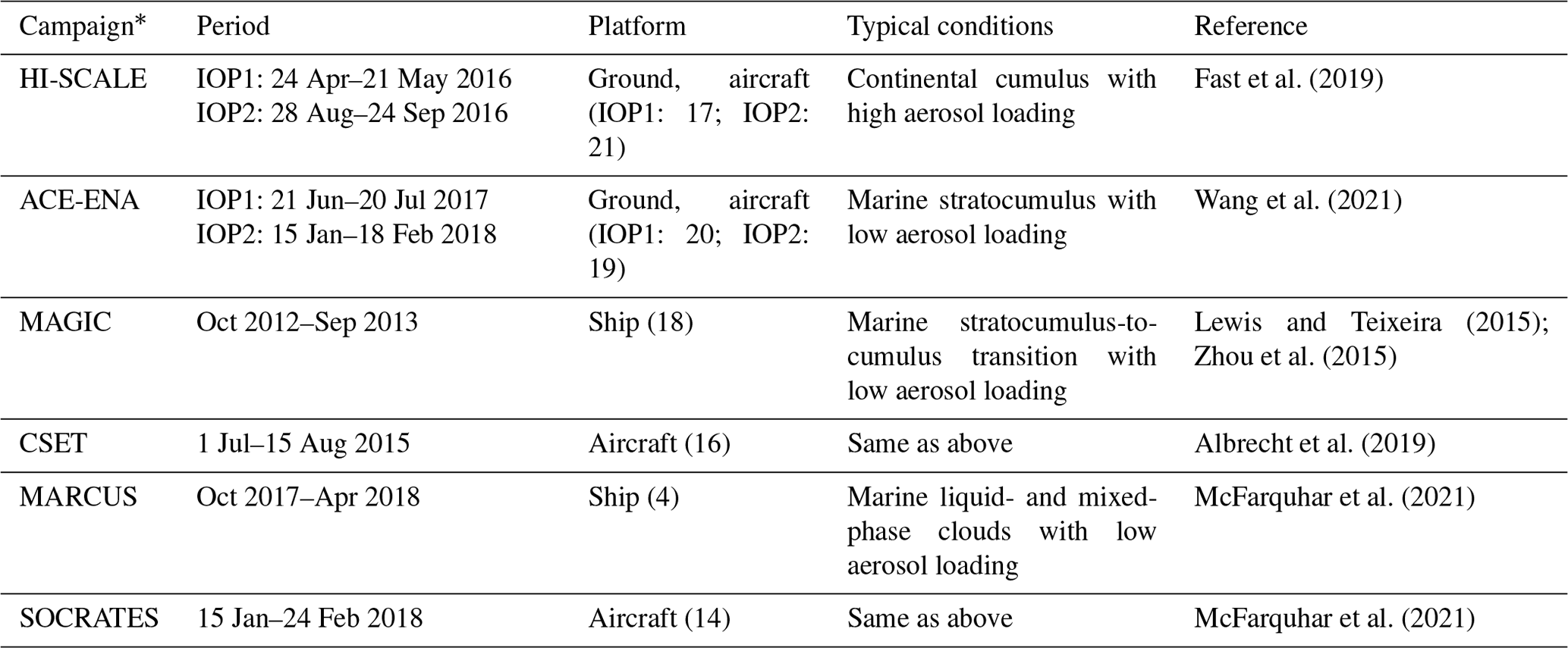
^* The full names of the listed field campaigns are as follows: HI-SCALE – Holistic Interactions of Shallow Clouds, Aerosols and Land Ecosystems; ACE-ENA – Aerosol and Cloud Experiments in the Eastern North Atlantic; MAGIC – Marine ARM GCSS Pacific Cross-section Intercomparison (GPCI) Investigation of Clouds; CSET – Cloud System Evolution in the Trades; MARCUS – Measurements of Aerosols, Radiation and Clouds over the Southern Ocean; SOCRATES – Southern Ocean Cloud Radiation and Aerosol Transport Experimental Study.

2 Introduction of ESMAC Diags

The workflow of ESMAC Diags v1 is illustrated in Fig. 1. Most field campaign datasets are directly read by the diagnostics package. In some field campaigns, more than one instrument is used to measure aerosol size distribution over different size ranges. Therefore, we merge these datasets to create a more complete description of the size distribution. These data are introduced in Sect. 2.1. Model outputs are extracted at the ground sites and along the flight tracks or ship tracks. The simulation and preprocessing details are provided in Sect. 2.2. ESMAC Diags reads in these field campaign and model data with quality controls and generates a set of diagnostics and metrics (as listed in Sect. 2.3). The diagnostics package is designed to be flexible so that additional measurements and functionality can be included in the future. Figure 2 depicts the directory structure to illustrate the organization of the datasets and code. Most of the datasets used in ESMAC Diags are in a standardized network common data form (netCDF) format (NETCDF, 2021); however, some ARM aircraft measurements use different American standard code (ASCII) formats. Currently, the diagnostic package reads observational data directly from their original format. In the long term, we may standardize the observational data format in a similar manner as was done in the GASSP project (Reddington et al., 2017).

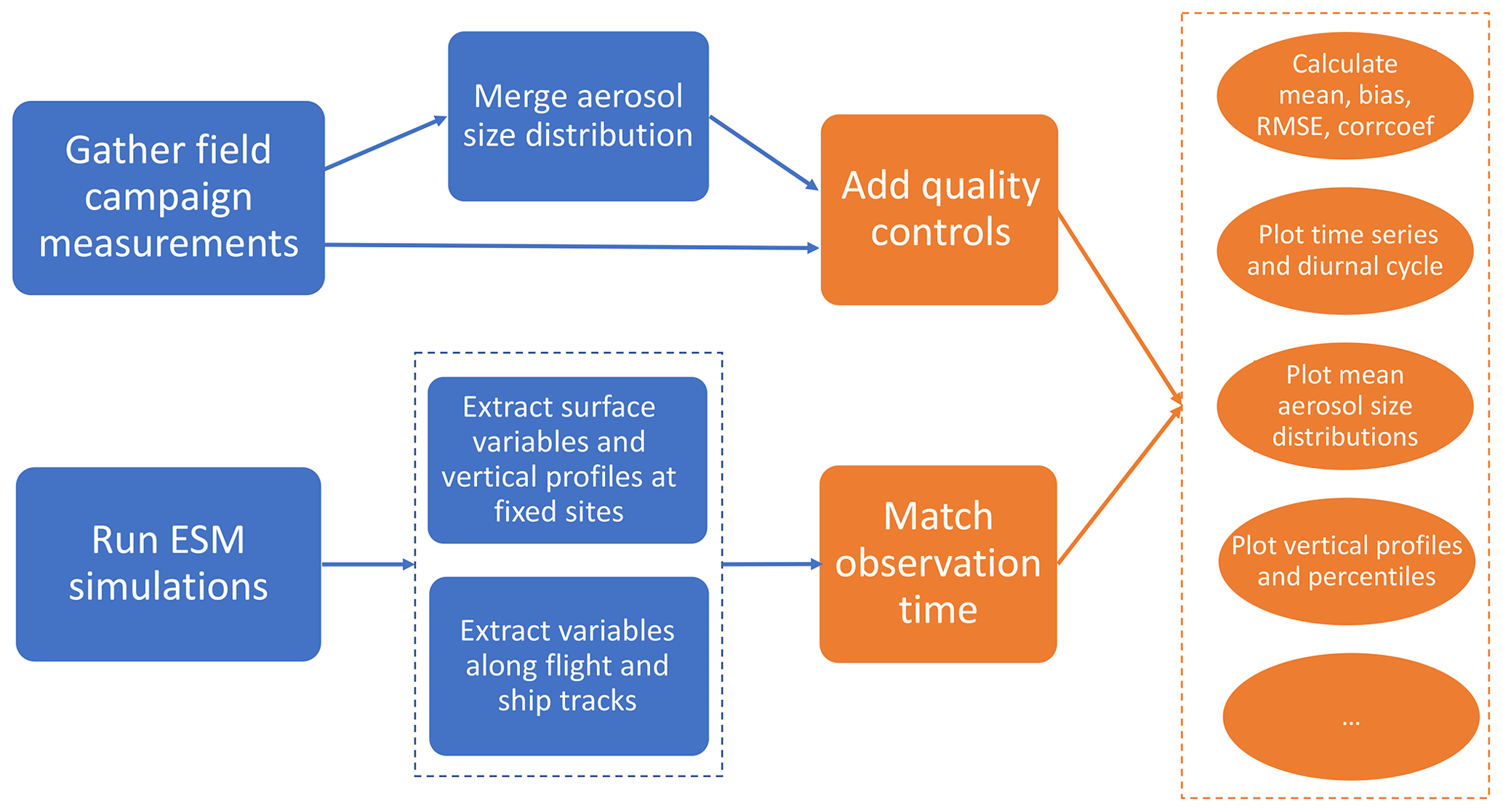
Figure 1 Workflow of ESMAC Diags. Data preprocessing and input are indicated by blue; diagnostics and plotting are indicated by orange.

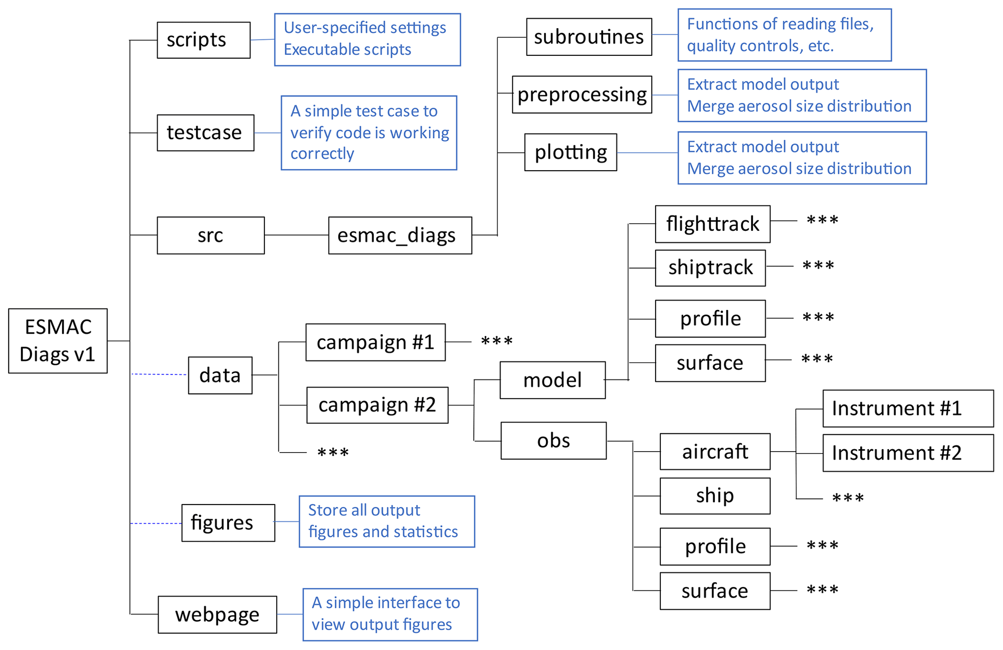
Figure 2 Structure of ESMAC Diags. The “scripts” directory contains executable scripts and user-specified settings. The “src” directory contains all source code, including code used to preprocess model output, read files, merge measurements from different instruments, compute observed versus simulated statistical relationships, and plot results. All observational and model data in the “data” directory are organized by field campaign. The diagnostic plots and statistics are put in the “figures” directory, also organized by field campaign. The “testcase” directory includes a small amount of input and verification data to test if the package is installed properly. The “webpage” directory provides an interface to view diagnostics figures. Boxes in blue describe the functions of the directory. Asterisks represent boxes that follow the same format as those shown in parallel.

2.1 Field observations and merged aerosol size distribution

We initially focus on four geographical regions where liquid clouds occur frequently and extensive measurements are available from ARM and other agencies: eastern North Atlantic (ENA), northeastern Pacific (NEP), central US (CUS, where the ARM Southern Great Plains, SGP, site is located), and Southern Ocean (SO). Aerosol properties also vary among these regions. Six field campaigns from these four test beds are selected in version 1 of ESMAC Diags (Table 1). HI-SCALE and ACE-ENA are based on long-term ARM ground sites with aircraft field campaigns sampling below, within, and above convective and marine boundary layer clouds, respectively, within a few hundred kilometers around the sites. CSET and MAGIC are field campaigns with respective aircraft and ship platforms sampling transects between California and Hawaii, which is an area characterized by a transition between stratocumulus- and trade-cumulus-dominated regions. SOCRATES and MARCUS are field campaigns with respective aircraft and ship platforms based out of Hobart, Australia. Aircraft transects during SOCRATES extended south to around 60^∘ S, while ship transects during MARCUS extended southwest from Hobart to Antarctica. The aircraft (black) and ship (red) tracks for these field campaigns are shown in Fig. 3.

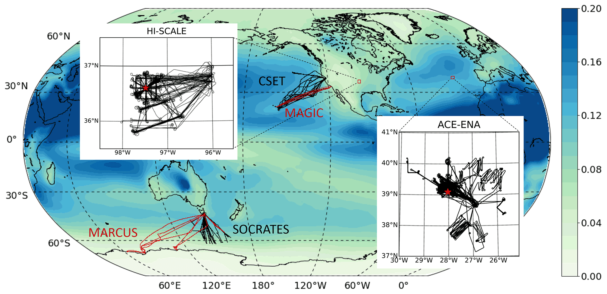
Figure 3 Aircraft (black) and ship (red) tracks for the six field campaigns. Overlaid is aerosol optical depth at 550 nm averaged from 2014 to 2018 simulated in EAMv1.

The instruments and measurements used in ESMAC Diags version 1 are listed in Table 2. All in situ measurements are converted to under ambient temperature and pressure. Note that some instruments are only available for certain field campaigns or failed operationally during certain periods; thus, model evaluation is limited by the availability of data collected in each field campaign. ARM data usually include quality flags indicating bad or indeterminate data. These flagged data are filtered out, except for surface condensation particle counter (CPC) measurements for HI-SCALE. CPC data flagged as greater than a maximum value (8000 cm⁻³) are retained, as aerosol loading can be higher than the abovementioned value during NPF events. This exception ensures a reasonable diurnal cycle, as shown in Sect. 3.3. For some data that do not have a quality flag, a simple minimum and maximum threshold is applied (e.g., a 500 cm⁻³ maximum threshold is used for each Ultra-High Sensitivity Aerosol Spectrometer, UHSAS, bin from the NCAR research flight measurements).

Table 2 List of instruments and measurements used in ESMAC Diags v1.

For some field campaigns (HI-SCALE and ACE-ENA), there are several instruments (e.g., fast integrated mobility spectrometer, passive cavity aerosol spectrometer probe, and optical particle counter for aircraft; scanning mobility particle sizer and nano-scanning mobility particle sizer for ground) measuring aerosol size distribution over different size ranges. These datasets are merged to create a more complete size distribution. In ESMAC Diags v1, aerosol “size” refers to the mobility and optical dry diameter of particles. The aerosol concentrations in the “overlapping” bins measured by multiple instruments are weighted by the uncertainty of each instrument based on the knowledge of the ARM instrument mentors. An example of the merged aerosol size distribution and individual measurements for one flight in ACE-ENA is shown in Fig. 4. Ranging from 10¹ to 10⁴ nm, the merged aerosol size distribution data account for the ultrafine, Aitken, and accumulation modes.

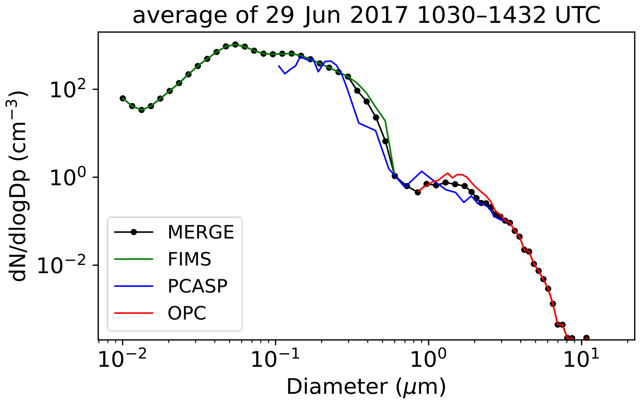
Figure 4 An example of a mean aerosol number distribution merged from the FIMS, PCASP, and OPC instruments for ACE-ENA aircraft measurements on 29 June 2017.

Although these measurements are considered as “truth” when evaluating ESMs, we note that they are subject to limitations and uncertainties due to factors such as theoretical/methodological formulations, sampling representativeness, instrumental accuracy and precision, imperfect calibration, and random errors. In addition, sampling volumes differ between observations and model output and are not reconcilable. It is difficult to quantify every aspect of observational uncertainty within the context of interpreting comparisons with model output, but we try to discuss some of them in this study to the best of our knowledge. Percentiles (either 25th–75th or 5th–95th) are used in some analyses of this study to approximate data variability that is likely to be much higher than measurement uncertainty.

2.2 Preprocessing of model output

In this study, we run EAMv1 from 2012 to 2018, covering all six field campaign periods introduced previously, with enough time for model spin-up. The model is configured to follow the Atmospheric Model Intercomparison Project (AMIP) protocol (Gates et al., 1999) with real-world forcings (e.g., greenhouse gases, sea surface temperature, and aerosol emissions). For each simulation year, we use the year 2014 emission data from Phase 6 of the Coupled Model Intercomparison Project (CMIP6), as the emission data do not cover years after 2014. The simulated horizontal winds are nudged towards the Modern-Era Retrospective analysis for Research and Applications, Version 2 (MERRA-2, Gelaro et al., 2017) with a relaxation timescale of 6 h. Using such a nudging configuration, previous studies (Sun et al., 2019; Zhang et al., 2014) have shown that the large-scale circulation is well constrained in the nudged simulation, especially for the mid- and high-latitude regions. The simulation uses a horizontal grid spacing of ∼ 1^∘ (NE30, the number of elements along a cube face of the E3SM High-Order Methods Modeling Environment, HOMME, dynamics core) with a 30 min time step. We saved hourly output for comparison with field campaign measurements. The diagnostics package post-processes 3-D model variables associated with aerosol concentration, size, composition, optical properties, precursor concentration, CCN concentration, and atmospheric state variables. The size of the output data is reduced by saving 3-D variables only over the field campaign regions. The model configuration and execution scripts are uploaded as an electronic supplement to this paper. Users can apply it in their own E3SM simulations (or output similar variables if running other models) to use this package.

We extracted model output along the aircraft (ship) tracks using an “aircraft simulator” (Fast et al., 2011) strategy to facilitate comparisons of observations and model predictions. At each aircraft (ship) measurement time, we find the nearest model grid cell, output time slice, and vertical level of the aircraft altitude (or the lowest level for ship) to obtain the appropriate model values. As both spatial and temporal mismatch exist between model output and field measurements, the evaluation focuses on overall statistics. We also calculate the aerosol size distribution from 1 to 3000 nm at 1 nm increments from the individual size distribution modes in MAM4 to facilitate comparisons with the observed aerosol number distribution that has different size ranges for different instruments. All of these variables are saved in separate directories according to the specific aircraft (ship) tracks, as indicated in Fig. 2.

2.3 List of diagnostics and metrics

Currently, ESMAC Diags produces the following diagnostics and metrics:

• mean value, bias, root-mean-square error (RMSE), and correlation of aerosol number concentration;

• time series of aerosol variables (aerosol number concentration, aerosol number size distribution, chemical composition, CCN number concentration) for each field campaign or intensive observational period (IOP) at the surface or along each flight (ship) track;

• diurnal cycle of aerosol variables at the surface;

• mean aerosol number size distribution for each field campaign or IOP;

• percentiles of aerosol variables by height for each field campaign or IOP;

• percentiles of aerosol variables by latitude for each field campaign or IOP;

• pie/bar charts of observed and predicted aerosol composition averaged over each field campaign or IOP;

• vertical profile of cloud fraction and liquid water content composite of aircraft measurements for each field campaign or IOP;

• time series of atmospheric state variables;

• aircraft and ship track maps.

In the next section, we will demonstrate these diagnostics and metrics by providing several examples.

3 Examples

Aerosol number concentration, size distribution, and chemical composition (that controls hygroscopicity) are key quantities that impact aerosol–cloud interactions, such as the activation of cloud droplets. Errors in model predictions of these aerosol properties contribute to uncertainties in aerosol direct and indirect radiative forcing. These aerosol properties vary dramatically depending on location, altitude, season, and meteorological conditions due to variability in emissions, formation mechanisms, and removal processes in the atmosphere. This section shows some examples to illustrate the usage of this diagnostics package in evaluating global models.

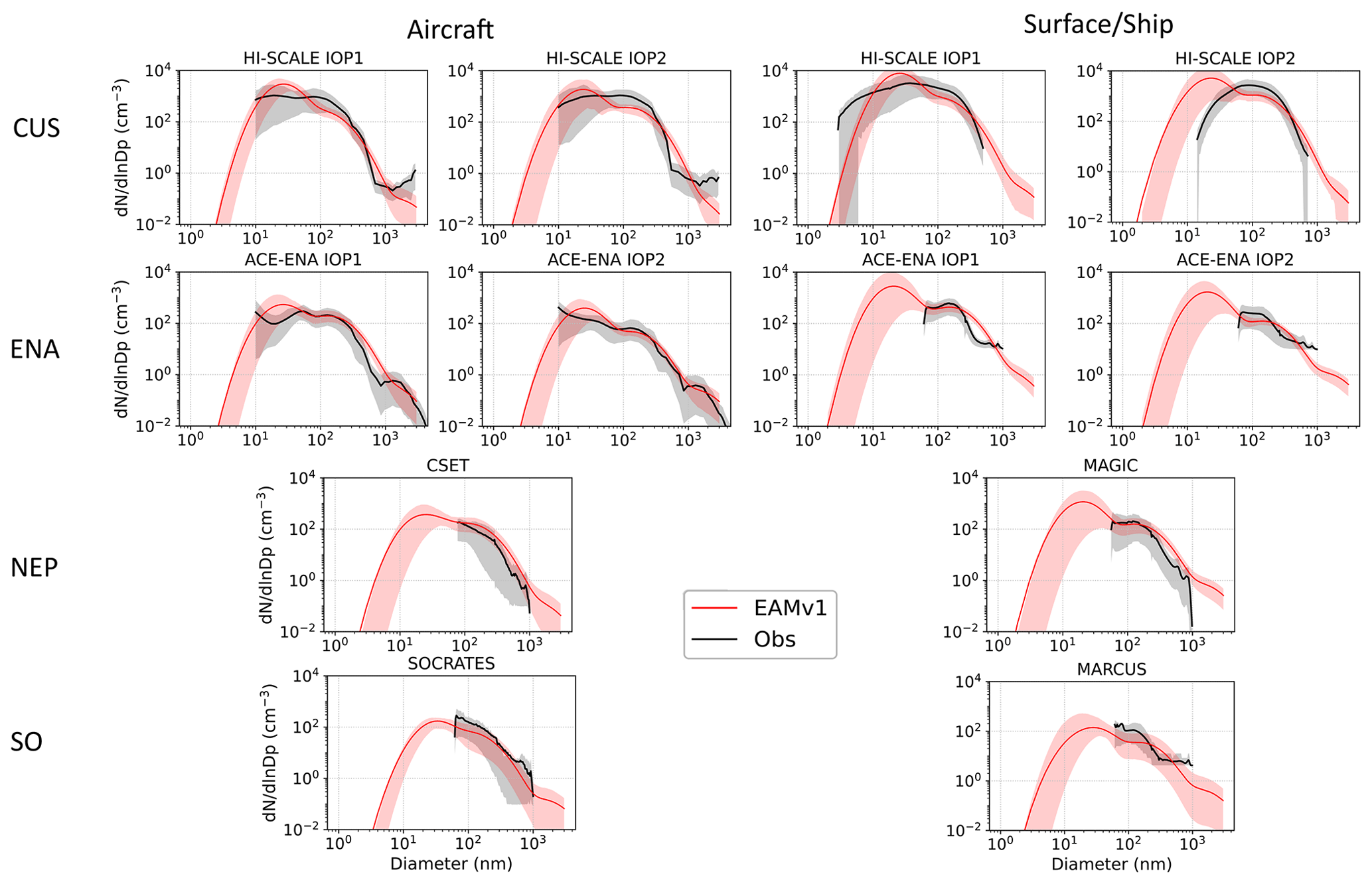
Figure 5 Mean aerosol number distribution averaged for each field campaign or IOP. Shadings denote the range between the 10th and 90th percentiles.

Table 3 Mean aerosol number concentration and interquartile range (25th and 75th percentiles, small numbers in parenthesis) for two size ranges averaged for each field campaign (or each IOP for HI-SCALE and ACE-ENA). Aircraft measurements 30 min after takeoff and before landing are excluded to remove possible contamination from the airport.

^* PCASP is available only on aircraft for HI-SCALE and ACE-ENA. UHSAS is available only in surface measurements for HI-SCALE and ACE-ENA as well as in other field campaigns. NA denotes not available.

3.1 Aerosol size distributions and number concentrations

Aerosol properties are highly dependent on location and season. Figure 5 shows the mean aerosol size distribution for each of the four test bed regions. For HI-SCALE and ACE-ENA, the two IOPs operated in different seasons are shown separately. Table 3 shows the mean aerosol number concentration from these field campaigns for two particle size ranges: >10 and >100 nm. The interquartile range (25th and 75th percentiles) is also shown to illustrate the variability in space and time. Among the four test bed regions, the CUS region has the largest aerosol number concentrations, as the other field campaigns are primarily over open ocean. Overall, EAMv1 overestimates Aitken-mode (10–70 nm) aerosols and underestimates accumulation-mode (70–400 nm) aerosols for the CUS and ENA regions, suggesting that processes related to particle growth or coagulation might be too weak in the model. Over the NEP region, EAMv1 overestimates aerosol number for particle sizes >100 and >10 nm (Table 3), both at the surface and aloft. Over the SO region, which is considered a pristine region with a low aerosol concentration, observations show a significant number of particles <200 nm in both aircraft and ship measurements (Fig. 5). The mean aerosol number concentration over the SO region is comparable to or even greater than the other ocean test beds (Table 3). In contrast, EAMv1 simulates a clean environment with the lowest aerosol number concentrations among the four regions. These types of comparisons demonstrate the need for additional analyses to understand why the SO has a similar aerosol number to other ocean regions and why EAMv1 cannot simulate this feature. The observed 75th percentiles are sometimes smaller than the mean value (Table 3), indicating a skewed aerosol size distribution with a long tail in the large aerosol size. EAMv1 usually produces a smaller interquartile range than the observations, likely because the current model resolution is too coarse to capture the observed spatial variability in aerosol properties.

Both the observed and simulated aerosol size distribution and number concentration show large variability during these field campaigns. Over the period of a few weeks or longer, aerosol number can vary by an order of magnitude between the 10th and 90th percentiles, especially for small particles (Fig. 5). Figure 6 shows the mean aerosol size distributions for two flight days during HI-SCALE: one with a large number of small (<70 nm) particles (14 May) and the other (3 September) with fewer small particles but more accumulation-mode (70–300 nm) particles. On both days, EAMv1 reproduces the observed planetary boundary layer height (PBLH) reasonably well with sufficient samples below and above the planetary boundary layer (PBL). On 14 May, EAMv1 reproduces the observed aerosol size distribution reasonably well, both within the PBL and in the lower free atmosphere. However, on 3 September, EAMv1 produces too many aerosols in the Aitken mode and too few accumulation mode aerosols in the PBL. In the free atmosphere, EAMv1 reproduces the lower concentration of Aitken-mode aerosols but still underestimates the accumulation mode. Such contrasting cases will be useful to help diagnose the specific processes contributing to model uncertainties in future analyses. This large day-to-day variability also indicates that long-term measurements are needed to avoid sampling bias in building robust statistics in aerosol properties. The next version of ESMAC Diags will be extended to include the available long-term ARM measurements at SGP, ENA, and other sites outside of the field campaign time periods.

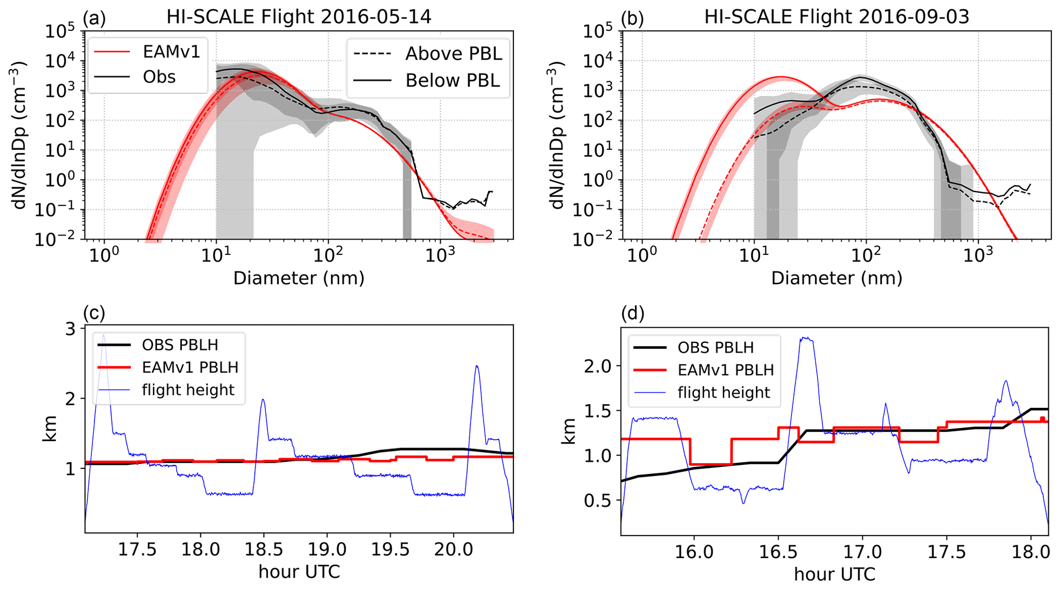
Figure 6 (a–b) Mean aerosol number distribution for two flights during HI-SCALE, (a) 14 May 2016 and (b) 3 September 2016, for data above (dashed line) and below (solid line) the observed PBLH. If there is cloud observed within a 1 h window of the sample point, the above-PBL sample needs to be above cloud top and the below-PBL sample needs to be below cloud base for the sample point to be chosen. Shadings represent the data range between the 10th and 90th percentiles. Relatively large particles with no shading indicate more than 90 % of samples with zero values. (c–d) Time series of the observed (black) and simulated (red) PBLH overlaid with flight height (blue) during the two flight periods. The observed PBLH is derived from Doppler lidar measurements.

3.2 Vertical profiles of aerosol properties

A research aircraft is the primary platform to provide information on the vertical variations in key aerosol properties that cannot be obtained accurately by remote sensing instrumentation. In this section, we show an example of evaluating vertical profiles of aerosol properties using aircraft measurements as well as illustrating the capability to evaluate multiple model simulations with ESMAC Diags. In addition to the standard EAMv1 simulation described in the previous section, we performed an EAMv1 simulation using the regionally refined mesh (RRM) (Tang et al., 2019). The model is configured to run with a horizontal grid spacing of ∼ 0.25^∘ over the continental US and ∼ 1^∘ elsewhere. The two model configurations are identical except for the higher spatial resolution (including primary aerosol emissions) in the RRM over the continental US. All aircraft measurements with a cloud detected simultaneously (cloud flag =1) were excluded.

Figure 7 shows vertical percentiles of aerosol number concentration, composition, and CCN number concentration among all of the HI-SCALE aircraft flights. Note that aircraft rarely flew above 3 km during HI-SCALE; thus, the sample size above that altitude is much smaller. The observed aerosol concentrations of number and chemical composition decrease with height, as the major sources of aerosols (anthropogenic, biogenic, and biomass burning) (Liu et al., 2021) are from precursors emitted near the surface and chemical formation within the PBL. EAMv1 generally simulates less variability than observations, except for sulfate. Overall, EAMv1 reproduces the observed mean aerosol number concentration for aerosol size >10 nm but underestimates the number of larger particles >100 nm during HI-SCALE (Table 3). The model also overestimates sulfate and underestimates organic matter concentrations when compared with aircraft AMS measurements. Its underestimation of the CCN number concentration is consistent with the underestimation of aerosol number concentration for diameters >100 nm but contrary to the overestimation of sulfate. A similar relationship is seen for ACE-ENA, which is described later in this section.

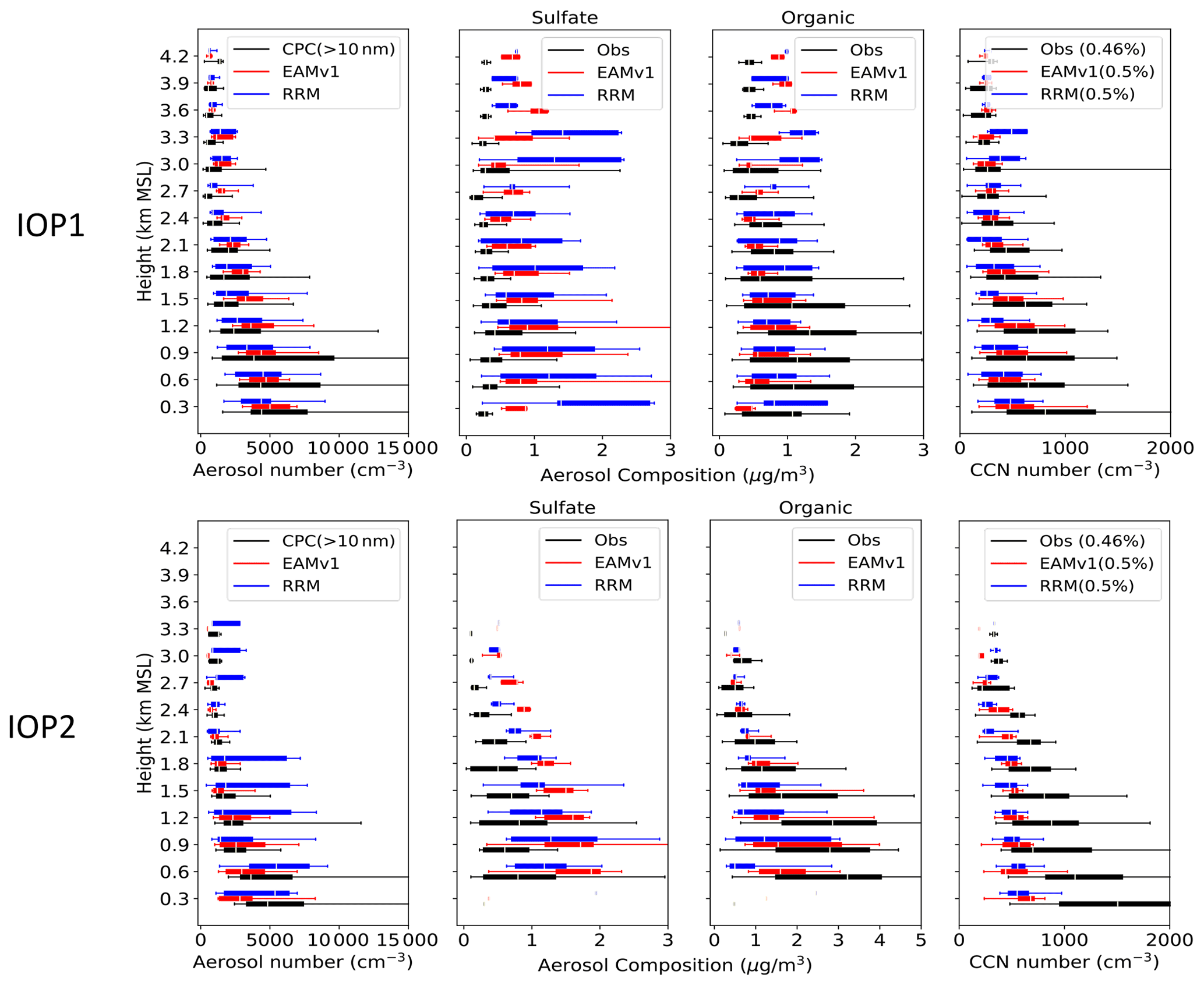
Figure 7 Vertical profiles of (from left to right) aerosol number concentration, mass concentration of sulfate, mass concentration of total organic matter, and CCN number concentration under the supersaturation in the parentheses for HI-SCALE (top) IOP1 and (bottom) IOP2. The percentile box represents the 25th and 75th percentiles, and the bar represents the 5th and 95th percentiles.

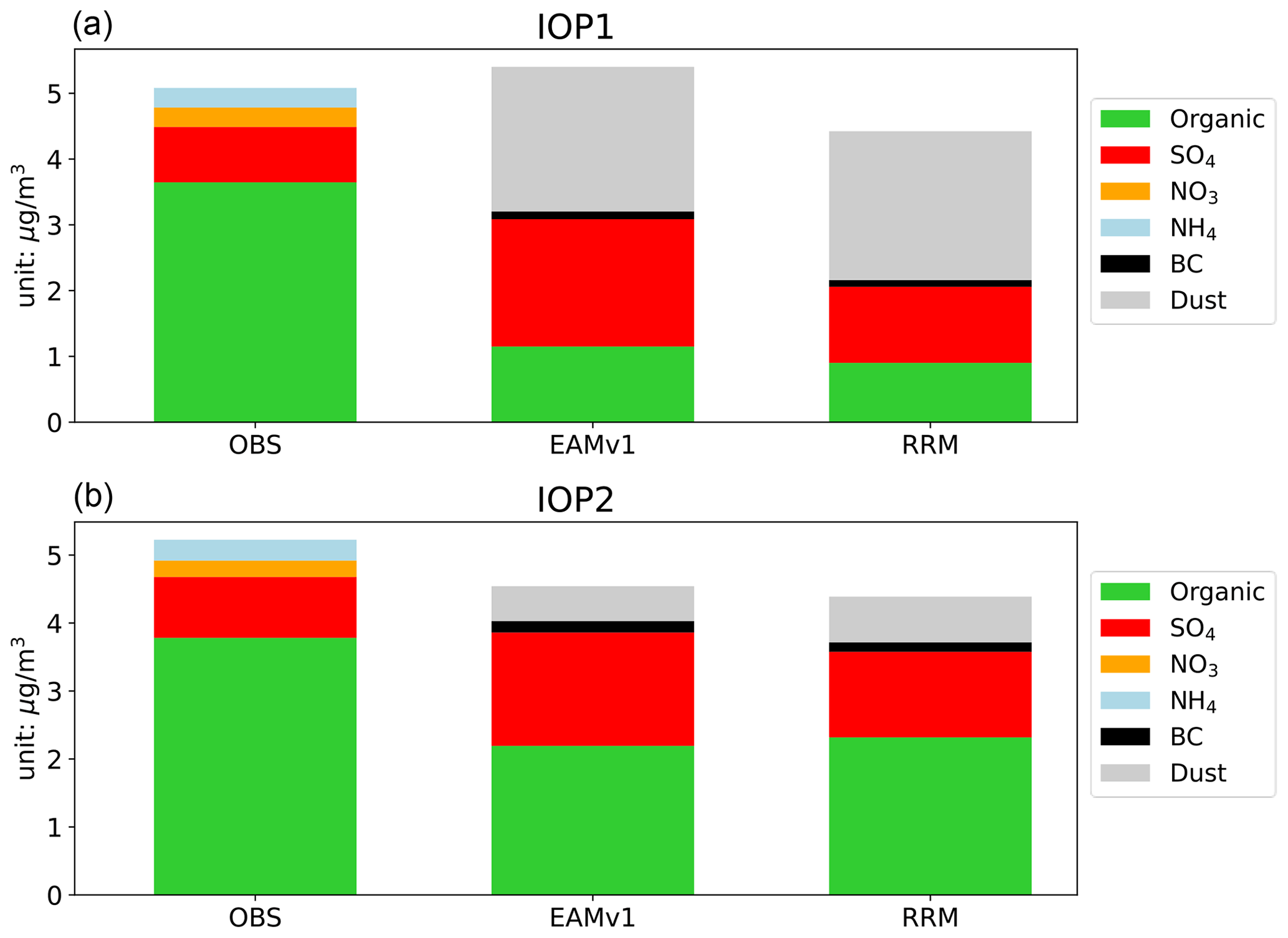
Figure 8 Bar plots of the surface average aerosol composition during HI-SCALE IOP1 (a) and IOP2 (b). Observations are obtained from an ACSM. Dust and black carbon (BC) are not measured in the observations. NO₃ and NH₄ are not predicted in EAMv1 and RRM.

The differences in sulfate and organic matter aloft are consistent with the longer-term surface measurement differences shown in Fig. 8, suggesting that this is a model bias. Note that near-surface measurements by aircraft are not always consistent with ground measurements (e.g., total organic matter in IOP1), which reflects the large spatial variability in aerosol properties associated with the aircraft flight paths up to a few hundred kilometers around the ARM site. The greater fraction of sulfate in EAMv1 suggests that the simulated aerosol hygroscopicity is likely higher than observed. Currently only these two species are available in both EAMv1 and AMS/ACSM observations for comparison purposes. Zaveri et al. (2021) recently added chemistry associated with NO₃ formation in MAM4, which is expected to be implemented in a future version of EAM.

Ongoing developments in E3SM will soon permit regionally refined meshes with grid spacings as small as ∼ 3 km as well as global convection-permitting simulations ($\mathrm{\Delta }\times \sim$ 3 km); therefore, this diagnostics package is designed to be flexible in scale to take advantage of higher-resolution ESM simulations that are more compatible with high-resolution in situ aerosol observations. This study demonstrates this ability by using a 0.25^∘ RRM simulation. Overall, the RRM analyzed here has similar biases as EAMv1, with differences that vary seasonally. The interquartile ranges in Fig. 7 show that the variability in organic aerosols and CCN from the EAMv1 and RRM simulations are similar. However, the variability in sulfate in RRM is larger than EAMv1 and observations during the spring IOP (IOP1). During the summer IOP (IOP2), the variabilities in sulfate in EAMv1, RRM, and observations are similar, and the sulfate concentrations from RRM are closer to observed values than EAMv1. Individual time series from the RRM simulation are still too smooth to capture the fine-scale variability in aerosols in observations (not shown). We expect E3SM to capture more fine-scale variabilities related to urban and point sources of aerosols and their precursors when the simulation grid spacing is further reduced to ∼ 3 km. A sensitivity study will be conducted when this high-resolution version of E3SM simulation becomes available.

Figure 9 Same as Fig. 7 but for ACE-ENA.

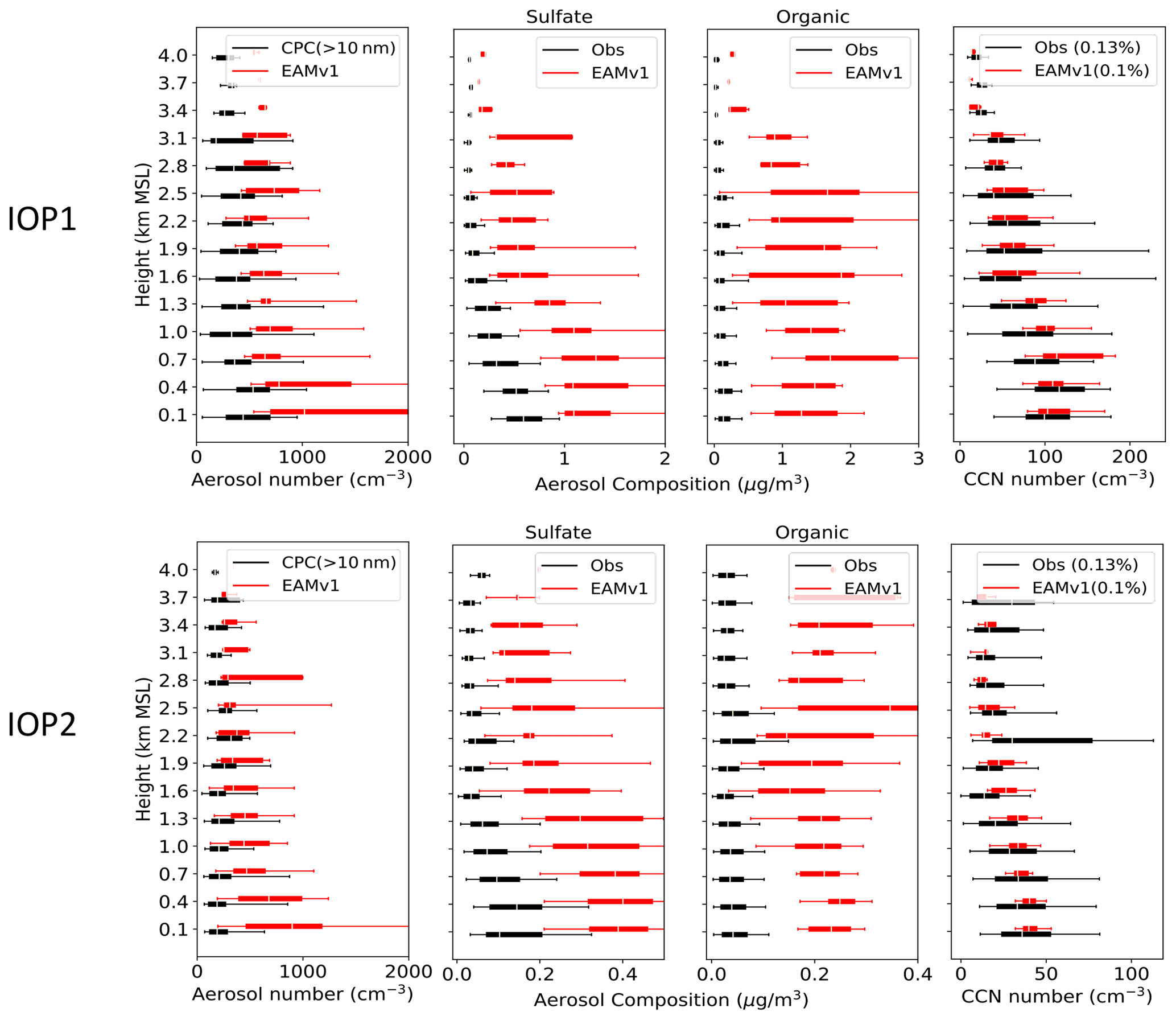
Figure 9 shows the vertical variation in percentiles of aerosol properties for ACE-ENA. The observed aerosol number concentrations, composition masses, and CCN number concentrations are much smaller than those for HI-SCALE, representing a cleaner ocean environment. EAMv1 produces larger mean values than the observations for all of these quantities. The overall variabilities in predicted aerosol number and concentrations of sulfate and organic matter are also greater than observed. Note that the observed variabilities for HI-SCALE are much larger than for ACE-ENA, indicating that EAMv1 has smaller location variation in aerosol variabilities. The observed total organic concentration shows a peak aloft between 1.6 and 2.2 km, corresponding to the level of the CCN number concentration peak. This implies that a major source of aerosols or precursors is free tropospheric transport (Zawadowicz et al., 2021). This peak in the total organic concentration aloft is also captured by the model.

Figure 10 Same as Fig. 8 but for ACE-ENA.

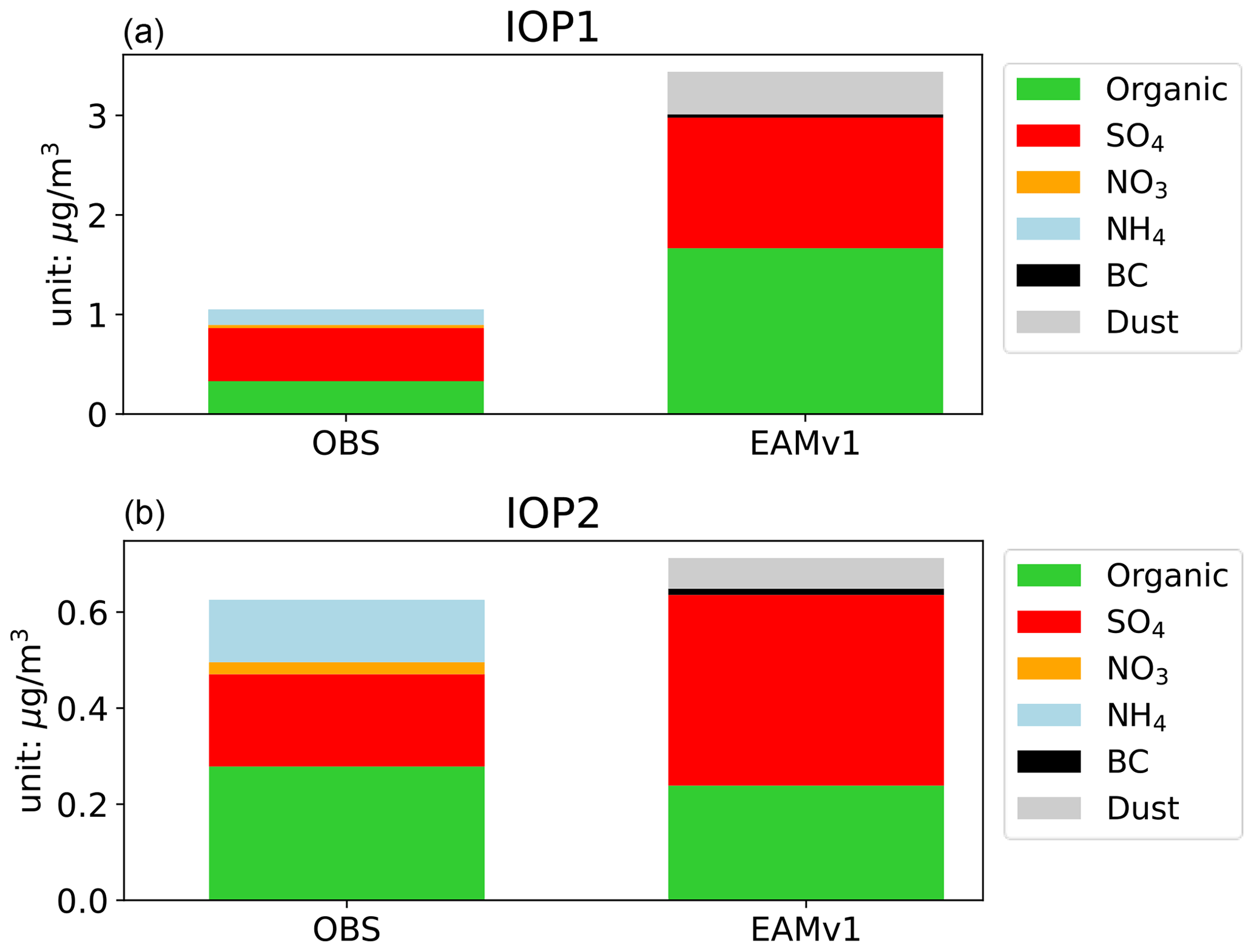
The bar plots of aerosol composition at the surface during ACE-ENA from the ACSM instrument and EAMv1 (Fig. 10) illustrate a similar bias in sulfate and organic mass as aloft. While the surface sulfate measurements are like those from the aircraft at the lowest altitudes, the observed surface organic matter is much higher than aloft, particularly during IOP2. The differences in these measurements may be due to local effects or possible contamination from aircraft, as the surface station is located near an airport on an island.

3.3 New particle formation events

Aerosol number concentrations and size distributions are highly impacted by NPF events (Kulmala et al., 2004), which further influence CCN concentration (e.g., Kuang et al., 2009; Pierce and Adams, 2009) and ultimately cloud properties. NPF and subsequent particle growth are frequently observed in the CUS region (Hodshire et al., 2016). As described by Fast et al. (2019) and shown in Fig. 11a, several NPF events were observed during the HI-SCALE spring IOP (IOP1). Large concentrations of aerosols smaller than 10 nm were observed, with the size growing larger over the next few hours. The average diurnal variation in the aerosol number distribution in Fig. 12a shows that NPF events usually occur during the morning between 12:00 and 15:00 UTC (06:00–09:00 LT, local time), followed by particle growth during the rest of the morning and afternoon. This variation is also seen in the diurnally averaged CPC measurements of aerosol diameters >3 and >10 nm (Fig. 12c), but diurnal changes in CCN number concentrations (Fig. 12d) are more modest.

Figure 11 Time series of (a) observed and (b) simulated surface aerosol number distribution during HI-SCALE IOP1. The observed aerosol number distribution is from merged nanoSMPS and SMPS data. Model data are cut off at 500 nm for comparison with observations.

Figure 12 Average diurnal cycle of surface (a) observed aerosol number distribution, (b) simulated aerosol number distribution, (c) aerosol number concentration for diameters >10 and >3 nm, and (d) CCN number concentration for supersaturations of 0.1 % and 0.5 % for HI-SCALE IOP1.

Various NPF pathways associated with different chemical species have been proposed and implemented in models. Two NPF pathways are considered in MAM4 in EAMv1: a binary nucleation pathway and a PBL cluster nucleation pathway. However, the current simulation does not reproduce the observed large day-to-day variability in small particle concentrations due to NPF. Instead, the model produces high aerosol concentrations between 10 and 100 nm almost all the time. It also fails to reproduce the large diurnal variability in the aerosol and CCN number concentration with a peak seen in the morning near 15:00 UTC (09:00 LT), 7 h earlier than the observed 22:00 UTC (16:00 LT) afternoon peak. Its overestimation of the aerosol number concentration for particle diameters >10 nm and its underestimation of the CCN number concentration is consistent with the information shown in Fig. 5. Several efforts are underway to improve the simulation of NPF by adding a nucleation mode in MAM4 to explicitly resolve ultrafine particles and by implementing new chemical pathways to simulate NPF following Zhao et al. (2020). ESMAC Diags is being used to evaluate these new model developments.

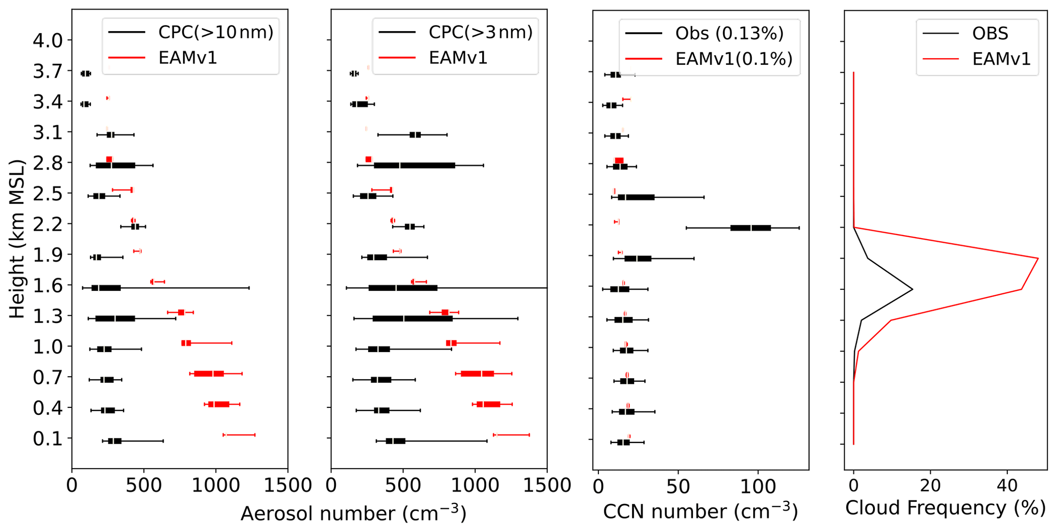
Figure 13 Vertical profiles of aerosol number concentration for diameters >10 and >3 nm, CCN number concentration, and cloud frequency measured by the 16 February 2018 flight in ACE-ENA. The percentile box represents the 25th and 75th percentiles, and the bar represents the 5th and 95th percentiles.

Figure 14 Percentiles of (a) air temperature, (b) grid-mean liquid water path (LWP), (c) aerosol number concentration for diameters >10 nm, and (d) aerosol number concentration for diameters >100 nm for all ship tracks in MAGIC binned by 1^∘ latitude bins. The percentile box represents the 25th and 75th percentiles, and the bar represents the 5th and 95th percentiles. The observed aerosol number concentrations for diameters >10 and >100 nm are obtained from CPC and UHSAS, respectively.

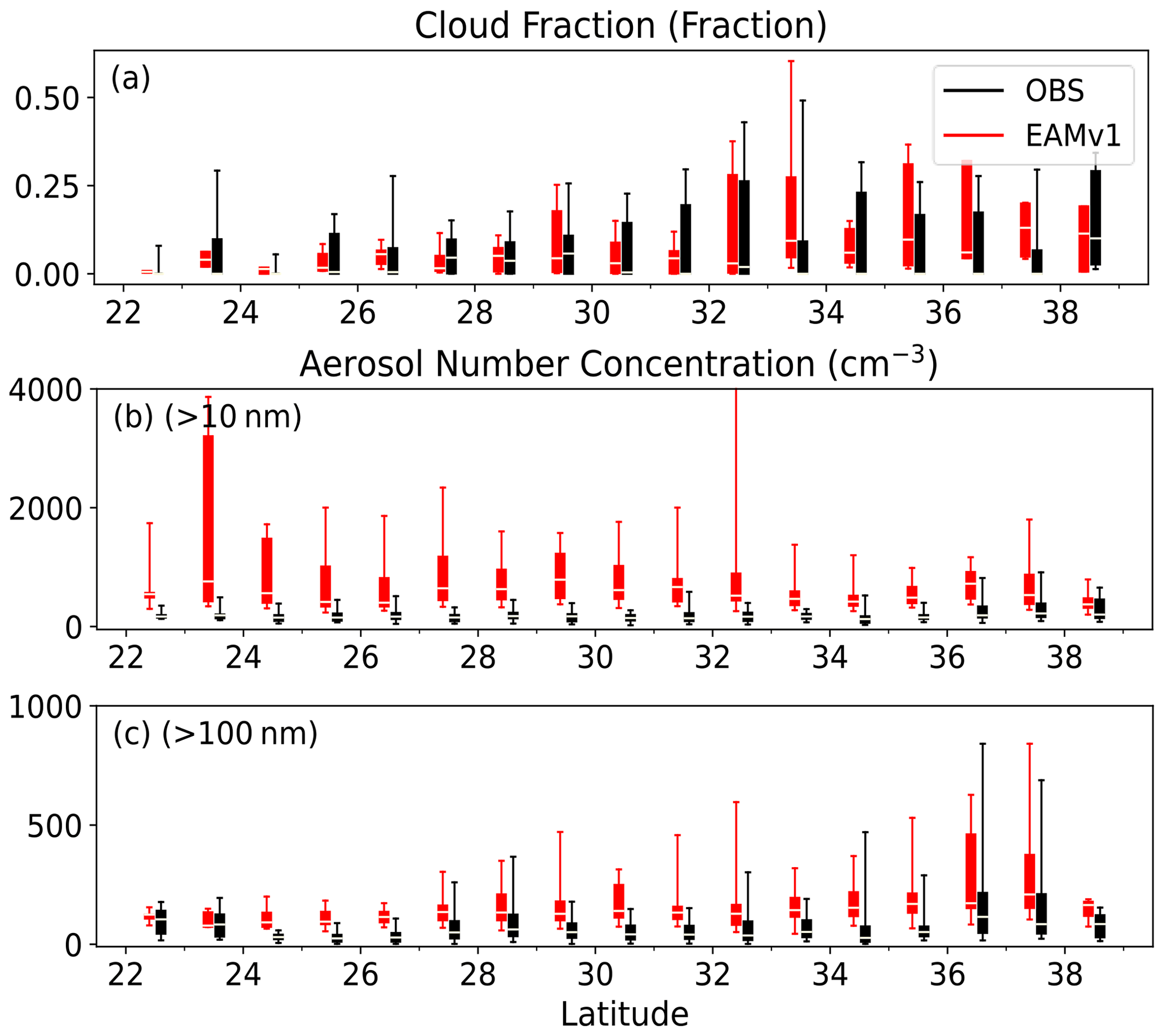
Figure 15 Percentiles of (a) cloud fraction, (b) aerosol number concentration for diameters >10 nm, and (c) aerosol number concentration for diameters >100 nm for all aircraft measurements between 0 and 3 km in CSET binned by 1^∘ latitude bins. The percentile box represents the 25th and 75th percentiles, and the bar represents the 5th and 95th percentiles. The observed aerosol number concentrations for diameters >10 and >100 nm are obtained from CNC and UHSAS, respectively.

Using aircraft measurements from ACE-ENA, Zheng et al. (2021) recently found evidence of NPF events occurring in the upper part of the marine boundary layer between broken clouds following the passage of a cold front. The 16 February 2018 is identified as a typical NPF day in Zheng et al. (2021). The vertical profiles of aerosol number and CCN concentrations measured by aircraft on 16 February 2018 are shown in Fig. 13. The NPF event and particle growth that occurred in the upper boundary layer are shown by the large mean and variance in the aerosol number concentration just below the base of the marine boundary layer clouds. EAMv1 could not simulate NPF events in the upper marine boundary layer on this day and other days during ACE-ENA, likely due to the lack of NPF mechanisms related to effective removal of existing particles, cold air temperatures, vertical transport of dimethyl sulfide (DMS), and high actinic fluxes in broken marine boundary layer clouds (Zheng et al., 2021). Similarly, the sharp increase in the CCN number just above the level of marine boundary layer clouds is not simulated.

3.4 Latitudinal dependence of aerosols and clouds

Unlike some field campaigns (i.e., HI-SCALE and ACE-ENA) in which aircraft missions were conducted over a relatively localized region with limited spatial variability in the meteorological conditions, ship and/or aircraft measurements over the NEP and SO test bed regions span regions >1500 km (i.e., from California to Hawaii and from Tasmania to the far Southern Ocean, respectively). As shown in Fig. 3, there are large spatial gradients in EAMv1-simulated aerosol optical depth along these ship/aircraft tracks. In ESMAC Diags version 1, we include composite plots of aerosol and cloud properties binned by latitude to assess model representation of synoptic-scale variations.

The research ship (aircraft) from the MAGIC (CSET) field campaign in the NEP test bed traveled between California and Hawaii, where there is frequently a transition between marine stratocumulus clouds near California and broken trade cumulus clouds near Hawaii (e.g., Teixeira et al., 2011). Although ESMAC Diags v1 focuses primarily on aerosols, we show some basic meteorological and cloud fields here, as they are important to illustrate the transition of cloud regimes along the ship (aircraft) tracks. Additional cloud properties derived from surface and satellite measurements are not included in the current analysis, but they are being implemented in ESMAC Diags v2. Some of the meteorological, cloud, and aerosol properties along the ship (aircraft) tracks binned by latitude are shown in Fig. 14 (Fig. 15). Note that the cloud fraction in Fig. 15 is calculated as the cloud frequency in the aircraft observations and from the grid-mean cloud fraction in the model along the flight track. This is different from the classic definition of cloud fraction usually used for satellite measurements or models and is subject to aircraft sampling strategy. As the surface temperature increases from California to Hawaii (Fig. 14a), the cloud fraction (Fig. 15a) shows a decreasing trend southwestward, indicating the transition from stratocumulus to cumulus clouds. However, the ship-measured liquid water path (LWP, Fig. 14b) has no trend related to latitude, possibly because cumulus clouds at lower latitudes have a smaller cloud fraction but a larger LWP when clouds exist. EAMv1 shows decreasing trends in both cloud fraction and LWP from high to low latitudes along these tracks. It generally underestimates the LWP and overestimates the cloud fraction to the north of 30^∘ N. For aerosol number concentrations, EAMv1 produces too many aerosols compared with measurements, both at the surface (ship) and aloft (aircraft), consistent with the aerosol size distribution in Fig. 5 and the total number concentration in Table 3. However, EAMv1 does reproduce the increase trend in the accumulation-mode aerosol concentration approaching the California coast.

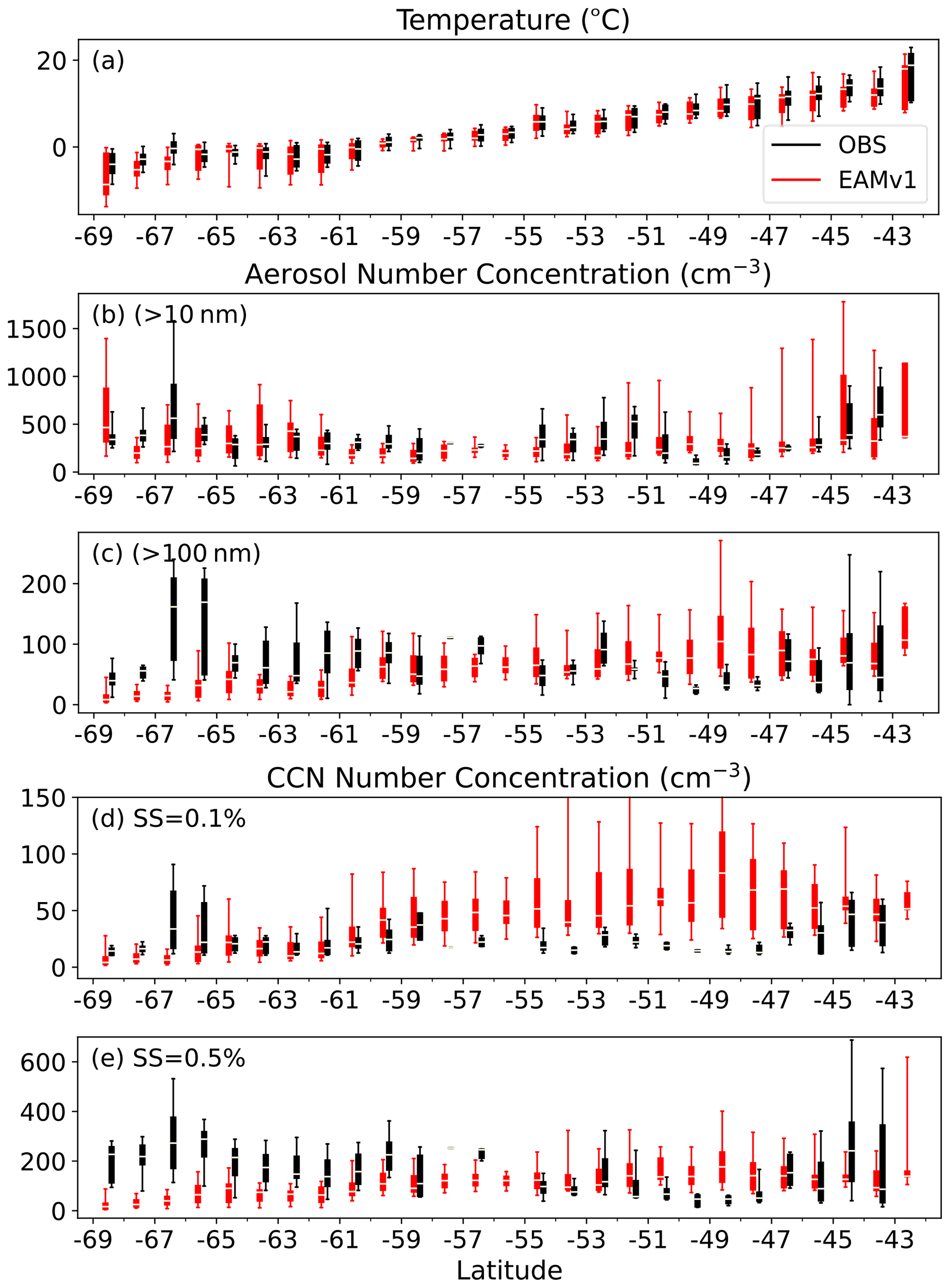
Figure 16 Percentiles of (a) air temperature, (b) aerosol number concentration for diameters >10 nm, (c) aerosol number concentration for diameters >100 nm, (d) CCN number concentration for SS=0.1 %, and (e) CCN number concentration for SS=0.5 % for all ship tracks in MARCUS binned by 1^∘ latitude bins.

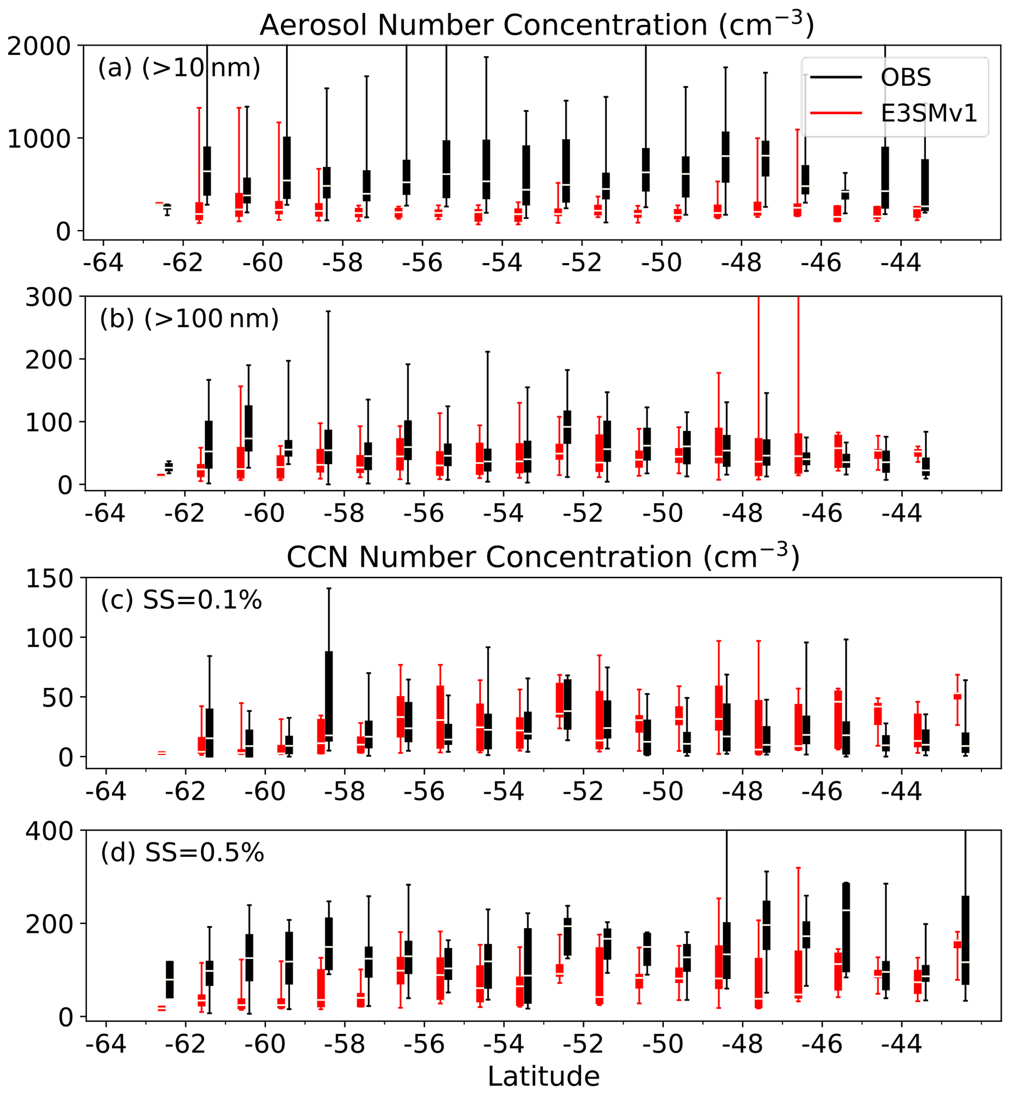
Figure 17 Percentiles of (a) aerosol number concentration for diameters >10 nm, (b) aerosol number concentration for diameters >100 nm, (c) CCN number concentration for SS=0.1 %, and (d) CCN number concentration for SS=0.5 % for all aircraft measurements between 0 and 3 km in SOCRATES binned by 1^∘ latitude bins.

Similar latitudinal gradients of aerosol and CCN number concentrations along ship tracks from MARCUS and aircraft tracks from SOCRATES are shown in Figs. 16 and 17, respectively. Over the SO region, NPF frequently occurs during austral summer when ample biogenic precursor gases (e.g., DMS) are released and rise into the free troposphere (McFarquhar et al., 2021; McCoy et al., 2021). Large values of ship-measured aerosol and CCN number concentration are observed near Antarctica, corresponding to the coastal biological emissions of aerosol precursors, and also occur to the north of 45^∘ S, indicating impacts from continental and anthropogenic sources. This is consistent with other studies (Sanchez et al., 2021; Humphries et al., 2021). EAMv1 underestimates the aerosol and CCN number concentration near Antarctica. This bias, which may be related to overly strong wet scavenging or insufficient NPF and growth, is commonly seen in many other ESMs (e.g., McCoy et al., 2020; McCoy et al., 2021). Aircraft flight paths during SOCRATES (Fig. 17) do not extend as far south as the ship measurements (Fig. 16). The observed aerosol properties generally have little latitudinal variation. EAMv1 underestimates the aerosol number concentration for particle sizes >10 nm and CCN number concentration with SS=0.5 %, but the predictions are closer to observed values for aerosol sizes >100 nm and CCN with SS=0.1 % (Fig. 17), consistent with the mean aerosol size distribution in Fig. 5. This indicates that the model performs better in simulating accumulation-mode particles than Aitken-mode particles over SO. These model aerosol biases are highly relevant when considering their interaction with clouds and radiations, which will be included in version 2 of ESMAC Diags.

4 Summary

A Python-based ESM aerosol–cloud diagnostics (ESMAC Diags) package is developed to quantify the performance of the DOE's E3SM atmospheric model using ARM and NCAR field campaign measurements. The first version of this diagnostics package focuses on aerosol properties. The measurements include aerosol number, size distribution, chemical composition, and CCN collected from surface, aircraft, and ship platforms; these measurements are needed to assess how well the aerosol life cycle is represented across spatial and temporal scales, which will subsequently impact uncertainties in aerosol radiative forcing estimates. Currently, the diagnostics cover the ACE-ENA, HI-SCALE, MAGIC/CSET, and MARCUS/SOCRATES field campaigns over the northeastern Atlantic, the continental US, the northeastern Pacific, and the Southern Ocean, respectively. The code structure is designed to be flexible and modular for future extension to other field campaigns or additional datasets. As there is no one instrument that can measure the entire aerosol size distribution, we have constructed merged aerosol size distributions from two or more ARM instruments to better assess the predicted size distributions. An “aircraft simulator” is used to extract aerosol and meteorological model variables along flight paths that vary in space and time. Similarly, the aircraft simulator is applied to ship tracks in which the altitude remains fixed at sea level.

Version 1 of the ESMAC Diags package provides various types of diagnostics and metrics, including time series, diurnal cycles, mean aerosol size distribution, pie charts for aerosol composition, percentiles by height, percentiles by latitude, and mean statistics of aerosol number concentration, among others. This allows for the quantification of model performance with respect to predicting the aerosol number, size, composition, vertical distribution, spatial distribution (along ship tracks or aircraft tracks), and new particle formation events. A full set of diagnostics plots and metrics for simulations used in this paper are available at https://portal.nersc.gov/project/m3525/sqtang/ESMAC_Diags_v1/forGMD/webpage/ (last access: 18 March 2022) and are archived as an electronic supplement to this paper. This article shows some examples to demonstrate the capability of ESMAC Diags to evaluate EAMv1-simulated aerosol properties. The diagnostics package also allows for multiple simulations in one plot in order to compare different models or model versions. Moreover, it can be applied to evaluate other ESMs with necessary modifications to fit different model output formats.

Because in situ aerosol measurements are usually collected at high temporal frequency (typically 1 s to 1 min) over fine spatial volumes, there is a spatiotemporal scale mismatch with the standard climate model resolution (usually 1^∘ grid spacing with hourly output). This is a limitation that cannot be completely overcome and must be accepted to perform the model–observation comparisons necessary for identifying shortcomings in the model representation of aerosol, cloud, and aerosol–cloud interaction processes that are the primary source of uncertainties in the prediction of future climate. As new versions of E3SM become available that have grid spacings as small as a few kilometers via regionally refined and convection-permitting global domains (e.g., Caldwell et al., 2021), spatiotemporal variabilities in aerosols at finer scales should be captured and should be more compatible with fine-resolution observations such that resolution impacts on statistical differences can be quantified. The diagnostics package will be applied to diagnose high-resolution model output when the data are available.

While the current version focuses on aerosol properties, version 2 of ESMAC Diags is being developed to include more diagnostics and metrics for cloud, precipitation, and radiation properties to facilitate the evaluation of aerosol–cloud interactions. These include inversion strength, above-cloud relative humidity, cloud–surface coupling, cloud fraction, depth, LWP, optical depth, effective radius, droplet number concentration, adiabaticity, albedo, and precipitation rate, among others. Long-term surface-based and satellite retrievals will also be used to provide better statistics in model evaluation and to address limitations related to data coverage and uncertainty. Analyses are being designed to quantify relationships between these variables and relate them to effective radiative forcing, which will be used to assess and improve model parameterizations. In the future, this diagnostics package may also be extended to include other field campaigns that provide valuable data on aerosol properties and cloud–aerosol interactions, such as the ARM Layered Atlantic Smoke Interactions with Clouds (LASIC, Zuidema et al., 2018), the NASA ObseRvations of Aerosols above CLouds and their intEractionS (ORACLES, Redemann et al., 2021), or the NASA Atmospheric Tomography Mission (ATom, Brock et al., 2019) campaigns. As an open-source package, ESMAC Diags can also be applied by any user to other ESMs with small modifications to model preprocessing.

While there are other efforts to develop model diagnostics packages, this diagnostics package provides a unique capability for detailed evaluation of aerosol properties that are tightly connected with parameterized processes. Together with other commonly used diagnostics packages, such as the ARM diagnostics package (Zhang et al., 2020), the DOE E3SM diagnostics package, and the PCMDI Metric Package (Gleckler et al., 2016), we expect to better understand the strengths and weaknesses of E3SM or other ESMs and to provide insights into model deficiencies to guide future model development. This includes studies that develop a better understanding of how various processes contribute to uncertainties in aerosol number and composition predictions and subsequent representation of CCN and aerosol radiative forcing estimates.