the Creative Commons Attribution 4.0 License.
the Creative Commons Attribution 4.0 License.
 | 16 May 2022
Description and evaluation of the community aerosol dynamics model MAFOR v2.0
Matthias Karl
Liisa Pirjola
Tiia Grönholm
Mona Kurppa
Srinivasan Anand
Xiaole Zhang
Andreas Held
Rolf Sander
Miikka Dal Maso
David Topping
Shuai Jiang
Leena Kangas
Jaakko Kukkonen
Numerical models are needed for evaluating aerosol processes in the atmosphere in state-of-the-art chemical transport models, urban-scale dispersion models, and climatic models. This article describes a publicly available aerosol dynamics model, MAFOR (Multicomponent Aerosol FORmation model; version 2.0); we address the main structure of the model, including the types of operation and the treatments of the aerosol processes. The model simultaneously solves the time evolution of both the particle number and the mass concentrations of aerosol components in each size section. In this way, the model can also allow for changes in the average density of particles. An evaluation of the model is also presented against a high-resolution observational dataset in a street canyon located in the centre of Helsinki (Finland) during afternoon traffic rush hour on 13 December 2010. The experimental data included measurements at different locations in the street canyon of ultrafine particles, black carbon, and fine particulate mass PM1. This evaluation has also included an intercomparison with the corresponding predictions of two other prominent aerosol dynamics models, AEROFOR and SALSA. All three models simulated the decrease in the measured total particle number concentrations fairly well with increasing distance from the vehicular emission source. The MAFOR model reproduced the evolution of the observed particle number size distributions more accurately than the other two models. The MAFOR model also predicted the variation of the concentration of PM1 better than the SALSA model. We also analysed the relative importance of various aerosol processes based on the predictions of the three models. As expected, atmospheric dilution dominated over other processes; dry deposition was the second most significant process. Numerical sensitivity tests with the MAFOR model revealed that the uncertainties associated with the properties of the condensing organic vapours affected only the size range of particles smaller than 10 nm in diameter. These uncertainties therefore do not significantly affect the predictions of the whole of the number size distribution and the total number concentration. The MAFOR model version 2 is well documented and versatile to use, providing a range of alternative parameterizations for various aerosol processes. The model includes an efficient numerical integration of particle number and mass concentrations, an operator splitting of processes, and the use of a fixed sectional method. The model could be used as a module in various atmospheric and climatic models.
- Article
(13562 KB) - Full-text XML
-
Supplement
(1085 KB) - BibTeX
- EndNote


Urban environments can contain high concentrations of aerosol particle numbers as a result of the emissions from local sources, most frequently vehicular traffic (Meskhidze et al., 2019), ship traffic (Pirjola et al., 2014), airports (Zhang et al., 2020), industrial emissions (Keuken et al., 2015), or all of these sources (Kukkonen et al., 2016). The majority of the urban aerosol particles – in terms of number concentration – are ultrafine particles (UFPs), having aerodynamic diameters less than 100 nm (e.g. Morawska et al., 2008). UFPs exhibit high deposition efficiency and large active surface area, and they are often associated with toxic contaminants, such as transition metals, polycyclic aromatic hydrocarbons, and other particle-bound organic compounds (Bakand et al., 2012). Owing to their small size, inhaled UFPs can penetrate deep in the human lungs, deposit in the lung epithelium, and translocate to other organs. Long-term exposure to UFPs negatively affects cardiovascular and respiratory health in humans (Wichmann and Peters, 2000; Evans et al., 2014; Breitner et al., 2011). Sub-micrometre soot particles emitted from diesel engines, mainly consisting of light-absorbing black carbon (BC), other combustion-generated carbonaceous materials, and condensed organics (Kerminen et al., 1997), often dominate the absorption of solar light by aerosols, thereby influencing the visibility in urban areas (Hamilton and Mansfield, 1991). The physicochemical characteristics of UFPs and their dynamic evolution also play an important role in changing the optical properties as they quickly coagulate with each other and larger particles or grow by the condensation of vapours into the size range of cloud condensation or ice nuclei, affecting the indirect climate effects of atmospheric aerosol by regulating cloud formation and cloud albedo, as well as changing the precipitation processes (Andreae and Rosenfeld, 2008).
In urban areas, the temporal variation and spatial inhomogeneity of both the particle number (PN) and particulate matter (PM) concentrations are closely linked to local meteorology and traffic flows (e.g. Kumar et al., 2011; Singh et al., 2014; Kukkonen et al., 2018). For example, particle concentrations in street canyons can be several times higher than in unobstructed locations. PN concentrations in a street canyon depend upon traffic characteristics, building geometry, turbulence that can be induced by traffic, the prevailing winds, and atmospheric stability (e.g. Kumar et al., 2009). However, measurements of particle number and size distributions in urban environments are scarce, and the complexity of the urban environment prevents extrapolation from single point measurements to the wider urban area.
A key question in applying aerosol process models is the scarcity of reliable and comprehensive emission data. Kukkonen et al. (2016) presented an emission inventory for particulate matter numbers (PNs) in the whole of Europe and in more detail in five target cities. The modelled PN concentrations (PNCs) were compared with experimental data on regional and urban scales. They concluded that it is feasible to model PNCs in major cities with reasonable accuracy; however, there were major challenges, especially in the evaluation of the emissions of PNCs. The rapid transformation of freshly emitted aerosol particles by condensation and evaporation, coagulation, and dry deposition was also found to pose challenges for dispersion modelling on the urban scale.
A substantial fraction of state-of-the-art chemical transport models contain treatments of aerosol processes (e.g. Kukkonen et al., 2012). However, only a limited number of urban dispersion models can deal with PN dispersion and processes affecting the particle size distribution, especially addressing the modelling of the dispersion of particles in complex urban terrain, such as street canyons (Gidhagen et al., 2004). This has been partly caused by the large effort toward model development that is necessary to implement size-resolved aerosol and particle dynamics models in urban modelling systems.
Modelling of particle transformation in parallel with plume dispersion is necessary to represent the evolution of the particle number and mass size distribution from the point of emission to the point of interest. Since the particle size and composition evolve on a short timescale, it is important to examine the evolution near the source at high spatial and temporal resolution. Modelling studies examining the evolution of particle emissions have used zero-dimensional (0-D) models (Vignati et al., 1999; Pohjola et al., 2003, 2007; Karl et al., 2016), one-dimensional (1-D) models (Fitzgerald et al., 1998; Capaldo et al., 2000; Boy et al., 2006), two-dimensional (2-D) models (Roldin et al., 2011), and three-dimensional (3-D) models (Gidhagen et al., 2005; Andersson et al., 2015). Jacobson and Seinfeld (2004) have modelled the near-source evolution of multiple aerosol size distributions with a 3-D chemistry-transport model (CTM) over a high-resolution limited-area grid; however, only a few minutes were simulated. Long-range aerosol transport models coupled with numerical weather prediction models can be used to trace the mass and number concentrations of aerosols from point source emissions at the surface and different vertical levels (Fountoukis et al., 2012; Sarkar et al., 2017; Chen et al., 2018). The size distribution of emissions in large-scale models can only be approximated because they need to take into account the size distribution of the primary emitted particles at the point of emissions and the ageing processes that occur at sub-model grid scales (Pierce et al., 2009). Higher temporal resolution is therefore necessary to better characterize primary and secondary particle sources. Computational fluid dynamics (CFD) models, notably building-resolving large eddy simulation (LES) models, are advantageous in simulating the airflow and dispersion of air pollutants in urban areas. Until now, only a few LES models have included modules for treating aerosol particles and their dynamics (Tonttila et al., 2017; Kurppa et al., 2019; Zhong et al., 2020). The implementation of aerosol dynamics into LES models increases their computational load tremendously.
Lagrangian approaches to the fluid flow are often employed in 0-D models that combine a vehicular plume model with an aerosol dynamics model in order to assess the impacts of coagulation, condensation of water vapour, and plume dilution of the particle number size distribution (e.g. Pohjola et al., 2007). On the urban scale, application of Lagrangian models is limited because of the large variability of emission sources and because they do not account for different wind speed or direction at different altitudes. However, the Lagrangian approach is advantageous for the examination of exhaust plumes in street environments, as it allows for the inclusion of more details on the representation of the aerosol dynamics and gas-phase chemistry than would be possible in a 3-D CTM. The traffic exhaust plume can be considered an isolated air parcel moving with the fluid flow, without mixing with other air parcels on the neighbourhood scale.
The Multicomponent Aerosol FORmation model MAFOR (Karl et al., 2011) is a 0-D Lagrangian-type sectional aerosol process model, which includes multiphase chemistry in addition to aerosol dynamics. It was originally developed to overcome the limitations of monodisperse models with respect to the simulation of continuous new particle formation in the marine boundary layer. Later, the model was extended with a module for dilution of particles in urban plumes with particles from background air (Karl et al., 2016). The aerosol dynamics module of MAFOR simultaneously solves the time evolution of particle number concentration and mass concentration of aerosol components in each size section in a consistent manner. The model allows for changes in the average density of particles and represents the growth of particles in terms of both the particle number and mass.
The aerosol dynamics in MAFOR are coupled to a detailed gas-phase chemistry module, which offers full flexibility for inclusion of new chemical species and reactions. Many aerosol dynamics models are designed to be coupled with a separate gas-phase chemistry module when implemented in atmospheric 3-D models. However, there are only a few other aerosol dynamics models for use in atmospheric studies that inherently integrate gas-phase chemistry together with aerosol processes as a function of time. Examples are ADCHEM (Roldin et al., 2011) and AEROFOR (Pirjola, 1999; Pirjola and Kulmala, 2001) that both use the kinetic code developed by Pirjola and Kulmala (1998), originally representing a modified EMEP chemistry scheme (Simpson, 1992). An advantage of AEROFOR is that it allows for multicomponent condensation to an externally or internally mixed particle population. AEROFOR has been applied to study aerosol dynamics and particle evolution under different atmospheric conditions such as arctic, boreal forest, and marine environments (e.g. Pirjola et al., 1998, 2002, 2004; Kulmala et al., 2000) as well as for the study of diesel exhaust particles under laboratory conditions (Pirjola et al., 2015). However, the model has limitations with respect to the treatment of particle-phase chemistry and does not solve mass concentration distributions as a function of time.
MAFOR has been proven to be particularly useful for studying changes in the emitted particle size distributions by dry deposition (to rough urban surfaces), coagulation processes, considering the fractal nature of soot aggregates, and condensation and evaporation of organic vapours emitted by vehicular traffic. The model is very versatile in its application: due to its modular structure, the model user can switch the different aerosol processes on and off or use alternative parameterizations for the same process, depending on the research question.
The first objective of this paper is to present the model's structure, the treatment of aerosol processes, the coupling to multiphase chemistry, and the main updates compared to the first publication of the model (version 1, in Karl et al., 2011). The second objective of the paper is the evaluation of the model performance of MAFOR version 2 with respect to its ability to predict particle and mass number size distributions.
Several of the new features of MAFOR version 2 were investigated in numerical scenarios and compared to reference data. Specifically, they included the evaluation of (1) the model's sectional representation of the aerosol size distribution in a scenario of new particle formation in urban areas (Case 1; Sect. S2 in the Supplement), (2) Brownian coagulation under the condition of continuous injection of nanoparticles (Case 2; Sect. S3), and (3) the dynamic treatment of semi-volatile inorganic gases by condensation and dissolution (Case 3; Sect. S4), and (4) a new parameterization for nucleation in the case of neutral and ion-induced particle formation (Appendix H).
The main performance evaluation of MAFOR version 2 is addressed in a real-world scenario of a street canyon environment in comparison with other aerosol process models and experimental data. In combination with the plume dispersion module, MAFOR version 1 has previously been evaluated against PN measurements at a motorway (Keuken et al., 2012) and against observed particle size distributions in the exhaust plumes of passenger ships arriving or leaving a ferry terminal (Karl et al., 2020). The real-world scenario in the present study focuses on the application of MAFOR version 2 for plume dispersion in a street canyon based on a published dataset of observations (Pirjola et al., 2012); from now on it is referred to as the Urban Case. Results from the MAFOR model are intercompared to the aerosol process models AEROFOR and SALSA (Kokkola et al., 2008). The relative importance of aerosol dynamic processes in this scenario is evaluated for the three models, with the dispersion–coagulation model LNMOM-DC (Anand and Mayya, 2015; Sarkar et al., 2020) as a reference for the relevance of coagulation. The performance of the aerosol dynamics models is evaluated based on defined criteria, such as statistical performance indicators, computational demand, and number of model output variables.
Section 2 describes the structure of the community aerosol dynamics model MAFOR version 2, the included physical and chemical processes, and their numerical solution. In addition, previous applications of the model are summarized and the new setup for modelling of the particle evolution in a street canyon is introduced. Section 3 presents the methods and the experimental data that are used for evaluation of the model in the Urban Case scenario. Section 4 discusses the results from the evaluation and from the comparison with other aerosol dynamics models.
MAFOR v2.0 is available as an open-source community aerosol model. The publication of MAFOR v2.0 as a community model is driven by the intention to provide both newcomers and experts in aerosol modelling with an easy-to-use stand-alone aerosol box model. A consortium of aerosol scientists guides the development of the community model. For application in atmospheric studies, apart from SALSA (Kokkola et al., 2008) and PartMC (Riemer et al., 2009), there is no other aerosol dynamics model to date that is available as open-source code. In recent years, several aspects of the MAFOR model have been revised and updated with aerosol process parameterizations published in the peer-reviewed literature. The main new features of MAFOR v2.0 compared to the original version (MAFOR v1.0, Karl et al., 2011) are the following:
-
coupling to the chemistry sub-model MECCA (Module Efficiently Calculating the Chemistry of the Atmosphere) of the community atmospheric chemistry box model CAABA/MECCA v4.0 (Sander et al., 2019);
-
extension of the Brownian coagulation kernel to consider the fractal geometry of soot particles, van der Waals forces, and viscous interactions;
-
inclusion of new nucleation parameterizations for neutral and ion-induced nucleation of H2SO4–water particle formation (Määttänen et al., 2018a, b) and H2SO4–water–NH3 ternary homogeneous and ion-mediated particle formation (Yu et al., 2020);
-
the Predictor of Nonequilibrium Growth (PNG) scheme (Jacobson, 2005a) implemented and linked with the thermodynamic module MESA (Zaveri et al., 2005b) of the MOSAIC (Model for Simulating Aerosol Interactions and Chemistry; Zaveri et al., 2008) to enable dynamic dissolution and evaporation of semi-volatile inorganic gases; and
-
absorptive partitioning of organic vapours to form secondary organic aerosol (SOA), following the formulation of the two-dimensional volatility basis set (2-D VBS; Donahue et al., 2011, within the framework of dynamic condensation and evaporation.)
The model can be run in three different types of operation: (1) simulation of an air parcel extending from the surface to the height of the planetary boundary layer (PBL) for multiple days along a given air mass trajectory or as a box model at a single geographic location, assuming a well-mixed boundary layer and clear-sky conditions (as a variation of this operation type, the multiphase chemistry during a fog cycle with pre-defined liquid water content and pH value of the fog and cloud can be simulated); (2) chamber experiment simulation assuming homogeneous mixing of constituents in a defined air volume for a given chamber geometry, considering sink terms and source terms of gases to and from chamber walls, deposition of particles to chamber walls, and constant dilution by replenishment of air; and (3) plume dispersion simulation that considers the evolution of the particle number and mass composition distributions in a single exhaust plume along one dimension in space by treating the transformation of emitted gases, condensing vapours, and particles concurrently with the dilution with background air during the spread of the plume volume. A special case is the simulation of dilution and ageing in a laboratory system for diesel exhaust using a simple parameterization for the dilution and cooling processes as described in Pirjola et al. (2015).
In the following sections, a detailed description of the physical and chemical processes and their numerical solution will be given. The focus is on presenting the new features that have been implemented after version 1.0. We begin with a review of the currently available aerosol process models in Sect. 2.1. Section 2.2 gives an overview of the structure and workflow of the MAFOR model. Section 2.3 describes the multiphase chemistry processes and each of the individual aerosol transformation processes in the model. Section 2.4 explains the dynamic treatment of semi-volatile inorganic gases in more detail. Section 2.5 presents SOA formation by absorptive partitioning of organic vapours according to the 2-D VBS. The numerical solution of the aerosol dynamics in the model is given in Sect. 2.6. A brief overview of previous applications of the model in plume dispersion scenarios is given in Sect. 2.7.
Throughout the paper, index q (q=1, … , NC) is used to denote chemical constituents, with NC being the number of constituents in the aerosol. Index i (i=1, … , NB) is used to denote the size section of the particle distribution, and NB is the number of size sections (bins). A list of acronyms and mathematical symbols is given in Appendix A.
2.1 Review of current aerosol process models
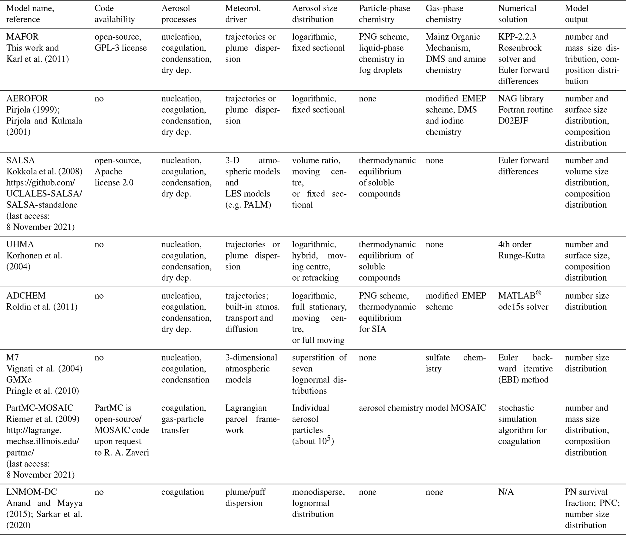
Table 1 provides a comparison of selected aerosol dynamics models that are currently used in studies of atmospheric aerosols. According to their representation of the particle size distribution, aerosol dynamics models can be divided into sectional, modal, monodisperse, and moment models (refer to Whitby and McMurry, 1997, for a detailed review).
Sectional models (Gelbard and Seinfeld, 1990; Warren and Seinfeld, 1985; Jacobson and Turco, 1995; Pirjola and Kulmala, 2001; Korhonen et al., 2004) place a grid on the independent variable space (e.g. particle diameter or volume). The aerosol size distribution is approximated by a finite number of size sections (bins) whose locations on the grid can either vary with time or be fixed. The first attempts to solve the stochastic collection equation for a droplet size distribution used a single-moment sectional approach, which tracks either particle number or particle mass. Later, two-moment sectional models were developed, which explicitly track both particle number (i.e. zeroth moment) and the mass concentration of aerosol components (i.e. first moment) in each size bin to predict the particle number and mass size distributions (Tzivion et al., 1987). The two-moment sectional approach can conserve both number and mass very accurately (Adams and Seinfeld, 2002). Two-moment sectional models have been implemented in global aerosol microphysics models for improving the understanding of the processes that control concentrations of cloud condensation nuclei (CCN), for example the climate model GISS-TOMAS (Lee and Adams, 2010) and the global offline CTM GLOMAP (Spracklen et al., 2005).
Modal models (Wright et al., 2001; Vignati et al., 2004) represent the particle distribution as a sum of modes, each having a lognormal or similar size distribution, typically described by mass, number, and width. Modal size distributions can be solved very efficiently, which makes them favourable candidates for global 3-D CTMs. However, the accuracy of the modal method is lower compared to the sectional method, especially if the standard deviation (width) of the modes is treated as constant (Zhang et al., 2002). In monodisperse models (Pirjola et al., 2003), all particles in each mode have the same size but can have different composition.
Karl et al. (2011)Pirjola (1999)Pirjola and Kulmala (2001)Kokkola et al. (2008)Roldin et al. (2011)Pringle et al. (2010)Anand and Mayya (2015)Sarkar et al. (2020)Table 1Comparison of selected zero-dimensional aerosol dynamics models for atmospheric simulation studies.
Moment models (McGraw, 1997) track a few low-order moments of the particle population but do not explicitly resolve the size distribution. Anand and Mayya (2009) have developed a formalism based on an analytical solution of the coagulation–diffusion equation for estimating the survival fraction of aerosols in dispersing puffs and plumes under the assumption of an initially Gaussian-distributed particle number concentration and spatially separable size spectra. The parameterization scheme has been further developed and is termed the Log Normal Method Of Moments – Diffusion Coagulation (LNMOM-DC) model, enabling the simultaneous treatment of aerosol coagulation and dispersion in an expanding exhaust plume.
The sectional aerosol dynamics model MAFOR allows for multicomponent condensation of vapours (sulfuric acid – H2SO4, methane sulfonic acid – MSA, ammonia – NH3, amines, nitric acid – HNO3, hydrochloric acid – HCl, water – H2O, and nine different organic compounds) to an internally mixed aerosol that includes all atmospherically relevant aerosol constituents, i.e. sulfate, ammonium, nitrate, methane sulfonate (MSAp), sea salt, soot, primary biological material, and mineral dust. The assumption of internally mixed particles, i.e. that all particles in the same size bin have the same chemical composition, lowers the accuracy in cases of high humidity in air because the ability to take up water can vary considerably for particles of the same size that have different composition (Korhonen et al., 2004). However, handling multivariate distributions that allow for same-sized particles with different hygroscopic properties involves large storage and computation requirements. The particle-resolved model PartMC-MOSAIC (Riemer et al., 2009; Tian et al., 2014) stores the composition of many individual aerosol particles (typically about 105) within a well-mixed computational volume. The computational burden is reduced by simulating the coagulation stochastically, assuming coagulation events are Poisson-distributed with a Brownian kernel.
The size-segregated aerosol model UHMA (Korhonen et al., 2004), another sectional aerosol dynamics model, has demonstrable good performance in reproducing new particle formation and solves the evolution of particle number and surface size distribution together with the composition distribution. In UHMA, the discretization of particle sizes is based on the volume of the particle core. A shortcoming of UHMA is that it does not explicitly solve the mass concentration change in individual aerosol components with time, whereas MAFOR takes into account the fact that the condensation or evaporation of an individual component results in the growth or shrinkage of the (total) mass concentration size distribution, affects the total aerosol mass, and moves the component's mass concentration distribution on the diameter coordinate.
The aerosol process models M7 (Vignati et al., 2004) and SALSA (Kokkola et al., 2008), partly owing to their computationally efficiency, have been implemented into the 3-D aerosol–climate model ECHAM5 (Bergman et al., 2012). SALSA is a sectional aerosol module developed with the specific purpose of implementation in large-scale models. It is part of the Hamburg Aerosol Model (HAM) (Stier et al., 2005) that handles the emissions, removal, and microphysics of aerosol particles and the gas-phase chemistry of dimethyl sulfide (DMS) within ECHAM5. Other implementation examples for SALSA in 3-D models are UCLALES-SALSA (Tonttila et al., 2017), PALM (Kurppa et al., 2019), and ECHAM-HAMMOZ (Kokkola et al., 2018). The focus of the implementation of SALSA is the description of the aerosol processes with sufficient accuracy, which is important for understanding aerosol–cloud interactions and their impacts on global climate. SALSA includes the aerosol microphysical processes nucleation, condensation, hydration, coagulation, cloud droplet activation, and oxidation of sulfur dioxide (SO2) in cloud droplets. The main advantage of SALSA is that particle size bin width does not have to be fixed, and lower size resolution can be used in the particle size range less affected by microphysical processes.
2.2 Model structure
Figure 1 illustrates the model structure of MAFOR v2.0. The model consists of three basic modules: (1) a chemistry module, (2) an aerosol dynamic module, and (3) a plume dispersion module. MAFOR is coupled with the chemistry sub-model MECCA v4.0 that allows the dynamic generation of new chemistry solver code and photolysis routines after adding new species and/or reactions to the chemistry mechanism. The newly generated code is packaged into a Fortran library that is included during the compilation of MAFOR, avoiding the need to build the MECCA interface each time when changes are made in the model code.
The chemistry module of MAFOR calculates time-varying gas-phase concentrations and aqueous-phase concentrations (in the droplet mode) by solving the non-linear system of stiff chemical ordinary differential equations (ODEs). The photolysis module JVAL (Sander et al., 2014) is used to calculate photolysis rate coefficients for photo-dissociation reactions. JVAL includes the JVPP (JVal PreProcessor), which pre-calculates the parameters required for calculating photolysis rate coefficients based on absorption cross sections and quantum yields of the atmospheric molecules. The Kinetic PreProcessor (KPP v2.2.3) (Sandu and Sander, 2006) is used to transform the chemical equations into programme code for the chemistry solver. The numerical integration of the ODE system of gas-phase and aqueous-phase reactions is done with Rosenbrock 3 using automatic time step control. The chemistry module also includes the emission and dry deposition of gases.
The aerosol dynamics module includes homogeneous nucleation of new particles according to various parameterizations, Brownian coagulation, condensation and evaporation, dry deposition, wet scavenging, and primary emission of particles. The composition of particles in any size bin can change with time due to multicomponent condensation and/or due to coagulation of particles. The aerosol dynamic solver updates number and component mass concentrations in the following order: (1) condensation and evaporation, (2) coagulation, (3) nucleation, (4) dry and wet deposition, and (5) emission. It returns an updated number concentration, updated component mass concentration per size bin, and updated gas-phase concentration of condensable and nucleating vapours.
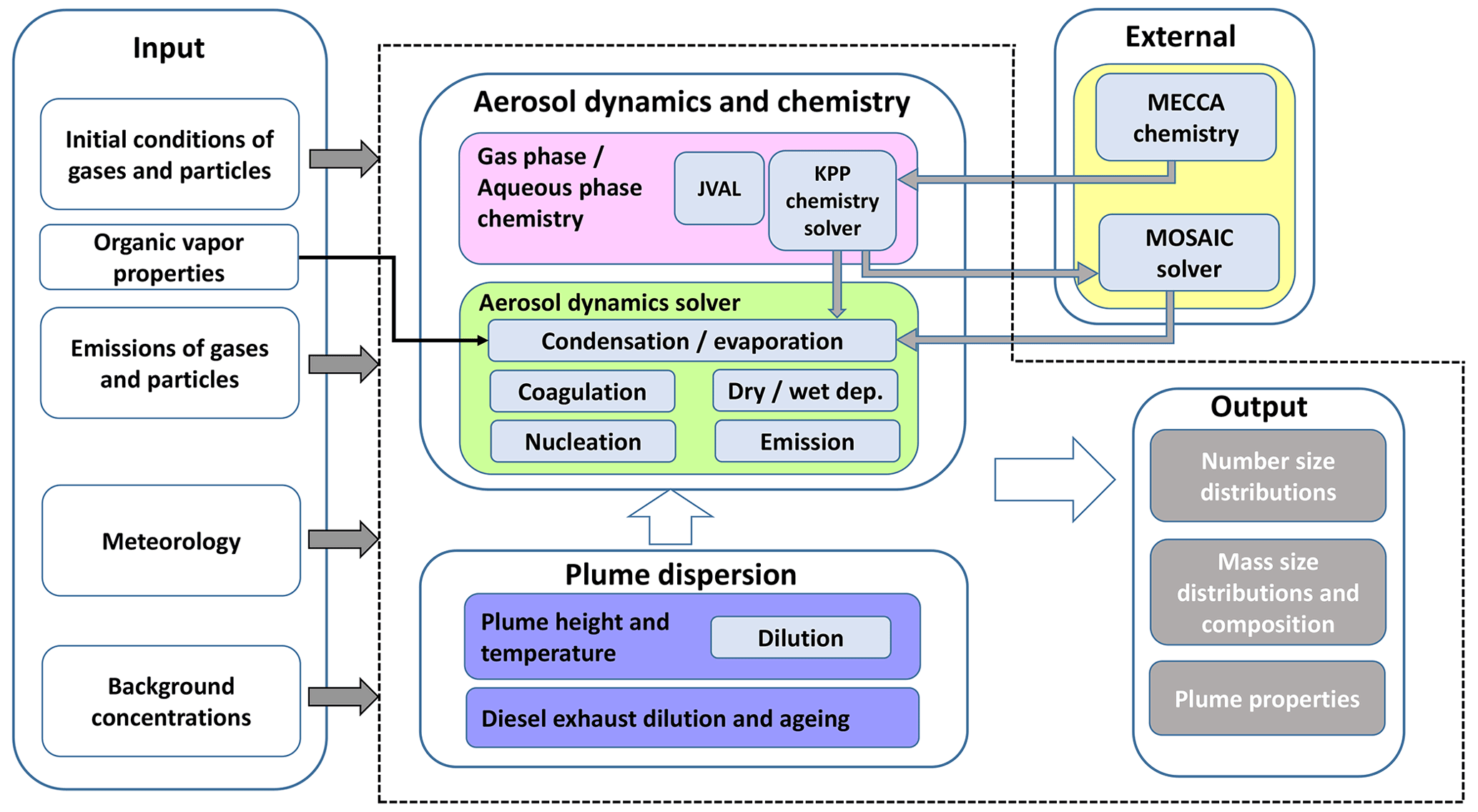
Figure 1Illustration of the model structure. Input data are on the left side. The area with a dashed outline contains the MAFOR model. External modules: interface to MECCA v4.0 and interface to MOSAIC solver (the models are not part of MAFOR). MECCA v4.0 is used to create the modules for the KPP chemistry solver, and the JVAL solver provides photolysis rate constants.
The plume dispersion module calculates the vertical dispersion of a Gaussian plume as a function of x (the downwind distance from the point of emission) and the dilution rate for the particle and gas concentrations in the plume. Temperature in the plume and the plume height varies with time according to prescribed dispersion parameters. In the case that the MAFOR model were included into a dispersion or climate modelling system, the plume dispersion model in Fig. 1 would be replaced by the advection–diffusion modules of that system.
The model starts with the initialization of the particle number and mass composition distributions as well as gas-phase concentrations. In the plume simulation, the aerosol distribution and gas-phase concentrations of the background air and dispersion parameters are initialized based on the user input. Meteorological conditions are updated on an hourly basis. It is possible to tailor the properties of the (lumped) organic compounds for the simulation to best represent the conditions in a chamber experiment or specific atmospheric region. As the model begins the integration over time, each process is solved using operator splitting in the following order: plume dispersion, chemical reactions, and aerosol dynamics. The changed gas-phase concentrations from the chemistry module are used in the aerosol dynamic module in the condensation and evaporation as well as nucleation processes. Pre-existing mass and number are input in the calculation of aerosol dynamic processes. The module first calculates the mass concentration of liquid water in each size section and consequently the wet diameter of particles, which is used for the calculation of aerosol dynamic processes. The dilution of particles is calculated after the number and mass concentrations of the current time step have been updated.
MAFOR has an interface to the MOSAIC model (Zaveri et al., 2008) for the treatment of condensation and evaporation of semi-volatile inorganic gases. This interface encapsulates a reduced version of the MOSAIC solver code in an external Fortran library. The thermodynamic module of MOSAIC is the Multicomponent Equilibrium Solver for Aerosols (MESA) model (Zaveri et al., 2005b). MESA is used here to calculate aerosol phase state, the activity coefficients of electrolytes in the aqueous solution, the equilibrium concentration of ammonium () in all size bins, and the parameters for dynamic growth by dissolution. An operator-split aerosol equilibrium calculation in MESA is performed to recalculate electrolyte composition and activity coefficients in each size bin. Finally, the MOSAIC interface provides the parameters required to determine the solubility terms in the PNG scheme (Jacobson, 2005b). In the PNG scheme, condensation (dissolution) and evaporation of HNO3, HCl, and H2SO4 are solved first. Following the growth calculation for all acid gases, NH3 is equilibrated with all size bins, conserving charge among all ions. In this method, ammonia growth is effectively a time-dependent process because the equilibration of NH3 is calculated after the diffusion-limited growth of all acids. The PNG scheme allows operator split to be done at a long time step (e.g. 150–300 s) between the growth calculation and the equilibrium calculation without causing oscillatory solutions when solving the condensation and evaporation of acid and base as separate processes (Jacobson, 2005b).
Two aspects in the implementation of the dynamic partitioning of inorganic and organic aerosol components in MAFOR v2.0 advance beyond the original concepts.
-
The condensation and dissolution of HNO3 and HCl were modified compared to the original PNG scheme. Condensation of the two gases to a particle size bin is applied when a solid is present in the bin using the minimum saturation vapour concentration. This leads to more nitrate mass to transfer to the aerosol phase compared to the original PNG scheme, which only considers solubility.
-
The coupling of the mass-based formulation from the 2-D VBS framework was implemented (Donahue et al., 2011) for organic aerosol phase partitioning, considering non-ideal solution behaviour, with the dynamics of organic condensation and evaporation according to a so-called hybrid approach, addressing the critical role of condensable organics in the growth of freshly nucleated particles.
2.3 Processes included in the model
2.3.1 Multiphase chemistry
The gas-phase and aqueous-phase chemistry mechanism is based on the MECCA chemistry sub-model of CAABA/MECCA v4.0 (Sander et al., 2019). In addition to the basic tropospheric chemistry it contains the Mainz Organic Mechanism (MOM) as an oxidation scheme for volatile organic compounds (VOCs), including alkanes, alkenes (up to four carbon atoms), ethyne (acetylene), isoprene, several aromatics, and five monoterpenes. Most of the VOC species of MOM are available for initialization in simulations with MAFOR. Diurnal variations of photolysis rates are based on Landgraf and Crutzen (1998) with the updates included in the JVAL photolysis module (Sander et al., 2014), such as updated UV–Vis cross sections as recommended by the Jet Propulsion Laboratory (JPL), evaluation no. 17 (Sander et al., 2011). The chemistry mechanism of MECCA was extended by a comprehensive reaction scheme for DMS adopted from Karl et al. (2007) and oxidation schemes of several amines: methylamine, dimethylamine, trimethylamine (Nielsen et al., 2011), 2-aminoethanol (Karl et al., 2012b), amino methyl propanol, diethanolamine, and triethanolamine. In total, the current chemistry mechanism of MAFOR v2.0 contains 781 species and 2220 reactions in the gas phase, as well as 152 species and 465 reactions in the aqueous phase. Initial concentrations of relevant gas-phase species, their dry deposition rate, and their emission rate can be provided by the model user.
The aqueous-phase chemistry is currently restricted to the liquid phase of coarse-mode aerosol (short: droplet mode). The composition of the liquid phase may be initialized with concentrations of the most relevant cations and anions. Transfer of molecules between the gas phase and the aqueous phase of coarse-mode aerosol and vice versa is treated by the resistance model of Schwartz (1986), which considers gas-phase diffusion, mass accommodation, and the Henry's law constants. The mass transfer coefficient km,q, a first-order loss rate constant, describes the mass transport of compound q from the gas phase to the aqueous phase:
where Dq is the molecular diffusion coefficient in the gas phase, cm,q is the molecular speed, αl,q is the mass accommodation coefficient (adsorption of the gas to the droplet surface), and rd is the droplet radius (mean radius of the monodisperse droplet mode). The first term represents the resistance caused by gas-phase diffusion, while the second term represents the interfacial mass transport. It is assumed that the liquid aerosol (cloud–fog droplet) behaves as an ideal solution and that no formation of solids occurs in the solution.
The change in gas-phase and aqueous-phase concentrations, Cg,q and Caq,q, of a (soluble) compound with time due to chemical reactions in a system with equilibrium partitioning is then described by
and
where Qg,q and Qaq,q are the gas-phase and aqueous-phase net production terms in chemical reactions, respectively, and LWC is the liquid water content. The dimensionless Henry's law coefficient, HA,q, for the equilibrium partitioning is independent of the liquid water content. Aqueous-phase partitioning parameters and aqueous-phase reactions are adopted from the MECCA chemistry module, extended with a treatment of organic molecules in the aqueous phase from Ervens et al. (2004) and amines in the aqueous phase from Ge et al. (2011).
2.3.2 Condensation and evaporation
The growth of particles through multicomponent condensation is implemented in MAFOR according to the continuum–transition regime theory corrected by a transitional correction factor (Fuchs and Sutugin, 1970). The scheme used for condensation and evaporation is the Analytical Predictor of Condensation (APC; Jacobson, 2005b) for dynamic transfer of gas-phase molecules to the particles over a discrete time step.
The difference between partial pressure of a condensable compound in air and vapour pressure on the particle surface is the driving force for condensation and evaporation in the model. Condensation and evaporation are solved by first calculating the single-particle molar condensation growth rate Iq,i (m3 s−1) for each compound q in each size bin i, given by
where υi is the particle volume, υg,q is the molecular volume of the condensing vapour, and Ceq,q (in µg m−3) is the saturation vapour concentration over a flat solution of the same composition as the particles. The factor is for conversion from mass-based to molecular units, where NA is the Avogadro constant ( mol−1) and MWq is the molecular weight of the condensing vapour (g mol−1). The diffusion coefficient Dq is estimated using an empirical correlation by Reid et al. (1987). The equilibrium saturation ratio of the condensing vapour, , is determined by the Kelvin effect and Raoult's law, Ke, with the molar fraction in the particle phase, γq,i, and the Kelvin term Ke.
The transitional correction factor βq,i is (Fuchs and Sutugin, 1970)
where αq is the mass accommodation (or sticking) coefficient of compound q. The default values for the accommodation coefficient are 0.5 for H2SO4 and 0.13 for MSA. The model user can replace these values by unity. The accommodation coefficient of organic vapours and all other inorganic vapours is assumed to be equal to unity. The Knudsen number is Kn , λv is the mean free path of vapour molecules, and ri is the particle radius.
The Kelvin effect due to curvature of particles is considered for the condensation and evaporation of all vapours. Inclusion of the Kelvin term reduces the condensation flux of vapours to particles smaller than 10 nm diameter in size. The Kelvin term Ke is expressed as
where R is the universal gas constant (R=8.3144 kg m2 s−2 K−1 mol−1), T is the air temperature (K), σq is the surface tension (kg s−2), ρL,q is the density of the pure liquid (kg m−3), and ri is particle radius in size bin i (m). Surface tension and density of the pure liquid for the condensing vapours are given in Table 2. The vapour pressure of the lumped organic compounds is modified by their molar fraction in the particle phase (according to Raoult's law) and by their molar volume and surface tension according to the Kelvin effect. The condensation flux of H2SO4 and MSA is corrected by the effect of hydrate formation following Karl et al. (2007). For organic vapours, the revised flux formulation by Lehtinen and Kulmala (2003) is used, which accounts for the molecule-like properties of the small particles, by modification of the transitional correction factor, Knudsen number, and mean free path.
The condensation of NH3 is coupled to the concentration of acid gases (H2SO4, HNO3, and HCl). If the NH3 concentration is at least 2-fold compared to the H2SO4 concentration, then two NH3 molecules are removed from the gas phase, assuming formation of ammonium sulfate [(NH4)2SO4]. If there is excess NH3 available for reaction with HNO3 to produce ammonium nitrate (NH4NO3), then each HNO3 molecule removes one NH3 molecule from the gas phase. NH3 can also react with HCl to produce ammonium chloride (NH4Cl). The formation of NH4NO3 and/or NH4Cl then determines the saturation vapour pressures of NH3, HNO3, and HCl. At equilibrium, the relation between the saturation concentration and the gas–solid equilibrium coefficients and , together with the mole balance equation, can be used to obtain the analytical solution for the saturation concentration of NH3 (i.e. ), as follows.
with
The saturation concentrations of HNO3 (i.e. ) and HCl (i.e. Ceq,HCl) are obtained accordingly. The reaction of alkylamines with HNO3 to alkyl ammonium nitrate is treated in analogy to the ammonia–nitric acid system. Alternatively, the PNG scheme, applicable across the entire relative humidity range, can be used to solve the growth by dissolution of HNO3 and HCl, as well as equilibration of NH3, as will be described in Sect. 2.4.
Saturation vapour pressures of the organic compounds are based on the C0 values (pure-compound saturation mass concentration) provided by the model user. Typical C0 values are shown in Table 2. Alternatively, the absorptive partitioning of organics is considered using the 2-D VBS method, as will be described in Sect. 2.5.
The gas-phase concentration of a condensing vapour with respect to condensation and evaporation as well as gas-phase chemistry is predicted according to
where Ni is the number concentration of particles (m−3). The second term on the right-hand side (RHS) in this equation represents the condensation–evaporation flux to a particle population, as defined in Eq. (3).
The change in the particle-phase mass concentration, mq,i, of the compound in each size bin with time due to condensation and evaporation is described by
with
where is the mass transfer rate (s−1) of gas to the particles of a size bin.
Table 2Molecular properties of the condensing vapours. Saturation concentration C0 is provided by the model user for the lumped organic compounds.

a Vehkamäki et al. (2002) using unity mole fraction of H2SO4.
b Temperature-dependent expression from Bolsaitis and Elliott (1990) using unity mole fraction of H2SO4.
c Temperature-dependent expression from Kreidenweis and Seinfeld (1998).
d Wyslouzil et al. (1991).
e Eq. (6) with and from Zaveri et al. (2008).
f Treated in analogy to the ammonia–nitric acid system.
g Temperature-dependent surface tension for pure succinic acid from Hyvärinen et al. (2006).
h Value for the organic vapours BSOV, BLOV, BELV, ASOV, ALOV, and AELV can be replaced by model user.
A non-iterative solution for the gas-phase and particle-phase concentration in each bin due to condensation over time is obtained by making use of the mass balance equation of the final aerosol- and gas-phase concentrations (Jacobson, 2005b). Details of the APC solver are given in Appendix B.
The condensation of H2O is accounted for by assuming the particles to be in equilibrium with the ambient water vapour. The uptake of water is calculated based on equilibrium thermodynamics (Binkowski and Shankar, 1995) using empirical polynomials (Tang and Munkelwitz, 1994) for the mass fraction of solute as a function of water activity. Polynomials for ammonium nitrate and ammonium sulfate are adopted from Chan et al. (1992). The water uptake of (soluble) semi-volatile organics is treated as sodium succinate with polynomials adopted from Peng and Chan (2001), and water uptake of sea salt particles is treated as sodium chloride (NaCl) according to Tang et al. (1997).
2.3.3 Nucleation
New particles are introduced into the atmosphere either by direct emission or by in situ nucleation of semi-volatile or low-volatility vapours. Nucleated particles (critical clusters) have initial sizes of the order of a few nanometres or less, which is much smaller than typical primary emission particle size ranges. Competition between growth by condensation and loss by coagulation determines the survival probability of a nucleated particle through a certain size range, usually up to 100 nm. Since freshly nucleated particles are small, they are highly diffusive and have a high propensity to collide with pre-existing particles. Nucleation in the atmosphere is a dynamic process that involves interactions of precursor vapour molecules, small clusters, and pre-existing particles (Zhang et al., 2012). However, the atmospheric nucleation mechanism is still surrounded with uncertainties. Several options of parameterized nucleation mechanisms can be chosen in the model; Table 3 provides a list of the available mechanisms.
Sulfuric acid is a highly probable candidate for atmospheric nucleation (Kulmala et al., 2004). Sihto et al. (2006) reported that nucleation-mode particle concentrations observed in a boreal forest (Hyytiälä, southern Finland) typically depend on H2SO4 concentration via a power-law relation with the exponent of 1 or 2. The proposed theory (Kulmala et al., 2006) of atmospheric nucleation by cluster activation (option 5) or kinetic nucleation (option 1) could be used to explain the observed behaviour. Charged clusters formed on ions are more stable and can grow faster than neutral clusters. Ion-mediated nucleation (IMN) considers the role of ubiquitous ions in enhancing the stability of pre-nucleation clusters (Yu and Turco, 2001). The ionization rate of air is about 2 ion pairs cm−3 s−1 at ground level and increases up to 20–30 ion pairs cm−3 s−1 in the upper troposphere. A constant ionization rate of 2 ion pairs cm−3 s−1 is used in all nucleation parameterizations that consider charged clusters in MAFOR. The combined nucleation scheme (option 7) is a combination of IMN and cluster activation (Karl et al., 2011; hereafter K2011) providing an upper estimate for the nucleation rate at low H2SO4 concentrations under tropospheric conditions.
Kulmala et al. (2006)Vehkamäki et al. (2002, 2003)Merikanto et al. (2007, 2009)Yu et al. (2018, 2020)Kulmala et al. (2006)Karl et al. (2012b)Karl et al. (2011)Karl et al. (2012a)Paasonen et al. (2010)Karl et al. (2012a)Paasonen et al. (2010)Karl et al. (2012a)Paasonen et al. (2010)Määttänen et al. (2018a, b)Pirjola et al. (2015)Henschel et al. (2016)Baranizadeh et al. (2016)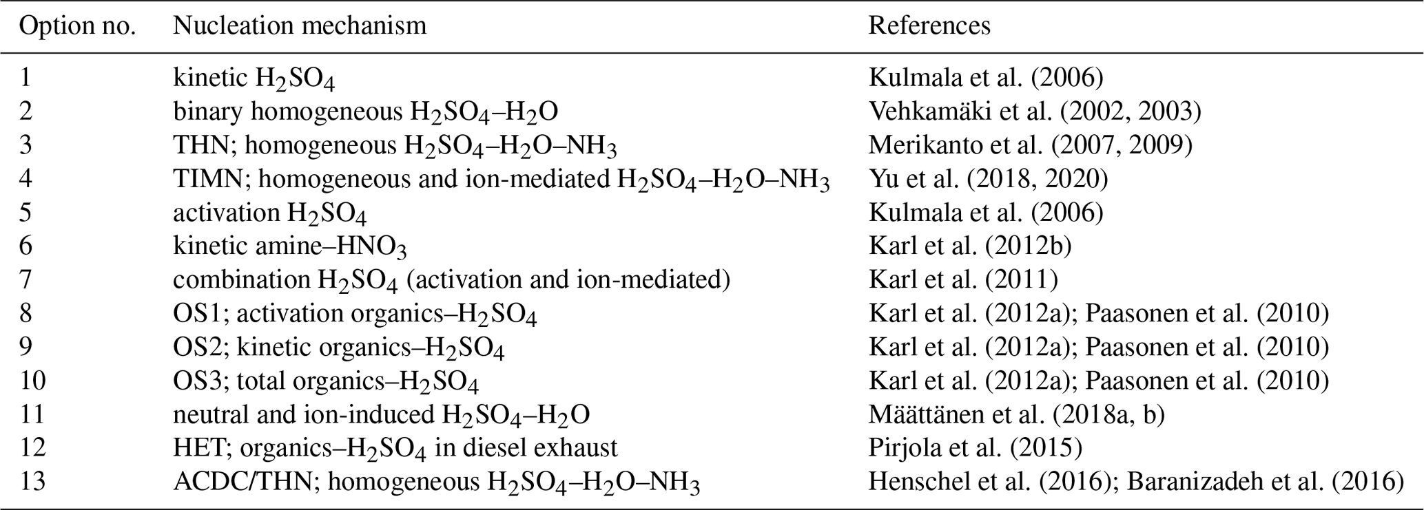
Binary homogeneous nucleation (BHN) of H2SO4–H2O may be the prevailing mechanism in the upper troposphere, and in some cases, classical BHN theory has successfully explained the observed formation rates of new particles (Weber et al., 1999; Pirjola et al., 1998). BHN is implemented in MAFOR based on the parameterization of Vehkamäki et al. (2002; hereafter V2002), which takes into account the effect of hydrate formation (Jaecker-Voirol et al., 1987; Noppel et al., 2002), extended to temperatures above 305 ∘C (Vehkamäki et al., 2003), which is suitable for predicting the particle formation rate at high temperatures in exhaust conditions (option 2).
Määttänen et al. (2018a; hereafter M2018) presented new parameterizations of neutral and ion-induced H2SO4–H2O particle formation (option 11) valid for large ranges of environmental conditions, which have been validated against a particle formation rate dataset generated in Cosmics Leaving OUtdoor Droplets (CLOUD) experiments. The implementation of the M2018 parameterization in MAFOR v2.0 has been tested in an urban background scenario (Case 1, T=288 K and RH =90 %), giving a maximum particle formation rate of 0.95 cm−3 s−1 when the H2SO4 concentration peaked at 5 × 107 cm−3 (Sect. S2). Only the ion-induced nucleation was active under these conditions.
Participation of a third compound in the nucleation process might explain discrepancies between H2SO4–water nucleation theories and laboratory measurements as well as field studies. Ternary homogeneous nucleation (THN) involving NH3 is a strong option due to the abundance of NH3 in the atmosphere and its ability to lower the partial pressure of H2SO4 above the solution surface. Merikanto et al. (2007) revised the classical theory of THN by including the effect of stable ammonium bisulfate formation (option 3), resulting in predicted nucleation rates that are several orders of magnitude lower compared to the original ternary nucleation model by Napari et al. (2002). More recently, the particle formation rates for THN have been updated based on simulations with the Atmospheric Cluster Dynamics Code (ACDC; Olenius et al., 2013) using quantum chemical input data (option 13). ACDC simulates the dynamics of a population of molecular clusters by numerically solving the cluster birth–death equations. Details of the ACDC simulations of the ternary H2SO4–NH3–H2O system can be found in Henschel et al. (2016; hereafter H2016). The ACDC/THN lookup table published by Baranizadeh et al. (2016) was implemented in MAFOR v2.0, allowing for the interpolation of particle formation rates under various conditions. MAFOR v2.0 also includes an implementation of the lookup table parameterization of ternary nucleation (TIMN, option 4) by Yu et al. (2020; hereafter Y2020). TIMN includes both ion-mediated and homogeneous ternary nucleation of H2SO4–NH3–H2O. At very low NH3 concentrations ([NH3] ≤105 cm−3), TIMN predicts nucleation rates according to BHN. Hence, the TIMN scheme offers the clear advantage that it can be directly applied to calculate nucleation rates in the whole troposphere in 3-D models.
Figure 2 compares the most relevant parameterizations for the particle formation from sulfuric acid nucleation under conditions relevant for the Urban Case scenario (T=262 K and RH =80 %) as a function of the H2SO4 concentration. The H2SO4 concentration for which the particle formation rate reaches Jnuc=1 cm−3 s−1 is 3.2 × 10⁶, 4.6 × 10⁶, 1.8 × 10⁷, 7.4 × 107 cm−3, and 6.0 × 10⁷ for K2011, M2018, Y2020 (at [NH3]=105 cm−3), H2016 (at cm−3), and V2002, respectively. K2011 gives the highest nucleation rates at low H2SO4 concentrations and shows an almost linear dependence on [H2SO4] because this parameterization does not consider kinetic limitation. The M2018 curve shows two turning points: the first at cm−3, when ion-induced nucleation reaches the kinetic limit, and the second at cm−3, when neutral BHN starts to dominate the total particle formation rate. The Y2020 parameterization is very sensitive to [H2SO4] at low H2SO4 concentrations but becomes insensitive to [H2SO4] at high concentrations due to the limitation of nucleation by the ionization rate. Particle formation rates from M2018 at high [H2SO4] are an order of magnitude higher than those predicted from the earlier V2002 parameterization.
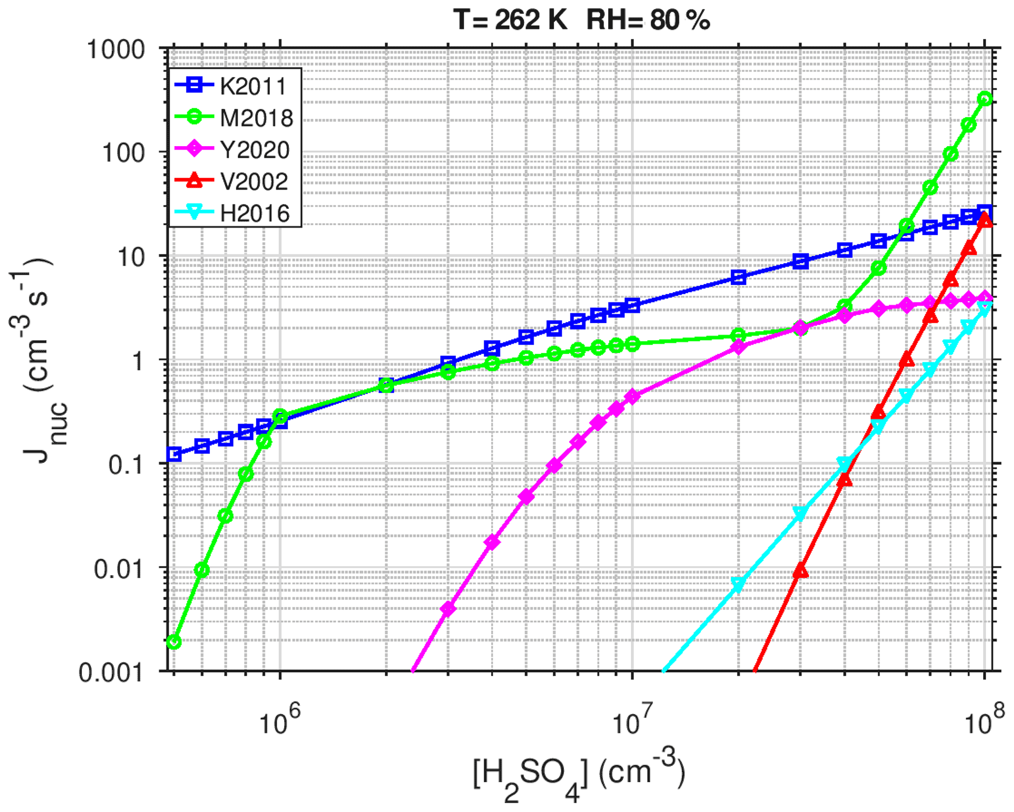
Figure 2Predicted nucleation rate Jnuc (cm−3 s−1) as a function of the concentration of H2SO4 (at T=262 K and RH =80 %) calculated with different parameterizations for particle formation through sulfuric acid: combined activation and IMN (K2011), neutral and ion-induced BHN (M2018), TIMN at cm−3 (Y2020), THN at cm−3 (H2016), and classical BHN (V2002).
Direct evidence for the participation of low-volatility organic vapours in the nucleation process comes from laboratory experiments (e.g. Metzger et al., 2010) that revealed higher nucleation rates compared to H2SO4 alone when the concentration of organics was increased. Paasonen et al. (2010) proposed different empirical parameterizations for the nucleation of organics–H2SO4 clusters, analogous to the kinetic and cluster activation mechanisms for H2SO4 clusters (Kulmala et al., 2006). From their proposed organics–H2SO4 nucleation mechanisms, three are included in MAFOR: (1) activation of non-identified clusters by both H2SO4 and organics (OS1, option 8), (2) homogeneous heteromolecular nucleation between H2SO4 and organic molecules combined with homogeneous homomolecular nucleation of H2SO4 according to kinetic nucleation theory (OS2, option 9), and (3) homogeneous nucleation of the organics in combination with the nucleation routes of OS2 according to kinetic nucleation theory (OS3, option 10). The same low-volatility organic vapour (SOA precursor BLOV) is used in all three parameterizations; it may also be involved in particle growth by condensation. Further nucleation options are organics–H2SO4 nucleation in diesel exhaust (HET, option 12), as suggested in Pirjola et al. (2015), and kinetic nucleation of amine–HNO3 (option 6) proposed by Karl et al. (2012b) for amine photo-oxidation experiments.
2.3.4 Coagulation
Coagulation of particles leads to a reduction in the total number of particles, changes the particle number size distribution and the chemical composition distribution, and leaves the total particle mass concentration unchanged. Coagulation is more efficient between particles of different sizes (inter-modal coagulation) than between same-sized particles (self-coagulation). The rate of coagulation is a product of size and diffusion coefficient: large particles provide a large collision surface, and the smaller particles have high mobility (Brownian motion). For instance, a particle of 10 nm diameter size coagulates about 170 times faster with a 1 µm particle than with another 10 nm particle (Ketzel and Berkowicz, 2004). Thermal coagulation of particles caused by Brownian motion of the particles is considered with an accurate treatment in MAFOR: a semi-implicit solution is applied to coagulation (Jacobson, 2005b). The (non-iterative) semi-implicit solution yields an immediate volume-conserving solution for coagulation with any time step. Brownian coagulation coefficients between particles in size bin i and j are calculated according to Fuchs (1964). For particles in the transition regime, the Brownian coagulation coefficient can be calculated with the interpolation formula of Fuchs (1964):
where δm is the mean distance from the centre of a sphere reached by particles leaving the sphere's surface and travelling a distance of the particle mean free path. Further, r is particle radius, Dm is the particle diffusion coefficient, and is the mean thermal speed of a particle with index i and j for the respective size bin. Details on the Brownian coagulation algorithm are given in Appendix C.
Brownian coagulation is well understood for coalescing particles of spherical shape. Soot particles in diesel exhaust, however, are fractal-like agglomerates that consist of nano-sized primary spherules. In the direct exhaust plume, the fractal shape of freshly emitted soot particles larger than 50 nm might increase their effective surface area that acts as a coagulation sink for the smaller particles (Ketzel and Berkowicz, 2004). The coagulation rate for agglomerate particles depends on particle mobility and the effective collision diameter; it is usually assumed that the collision diameter is equal to either the mobility diameter or the outer diameter (Rogak and Flagan, 1992).
The effect of fractal geometry on coagulation is treated in the model by considering the effect of shape on radius, diffusion coefficient, and Knudsen number in the Brownian coagulation kernel. It is assumed that the collision radius, rc, is equal to the outer radius, rf, of the agglomerate, defined as
where ns is the number of primary spherules in the aggregate, rs is the radius of spherules, and Df is the fractal dimension. The model user is asked to provide values for rs and Df for the fractal (soot) particles. In accordance with Lemmetty et al. (2008), the effective density of fractal (soot) particles larger than the primary spherules is expressed as
where Dp,i is particle diameter of size bin i, while ds and ρs are the diameter and density of the primary spherules (for soot: 1200 kg m−3), respectively.
The Brownian coagulation kernel is modified for fractal geometry with (Jacobson and Seinfeld, 2004)
with the mean distance, δm, from the particle's centre and the Knudsen number for air evaluated at the mobility radius. Here, the particle diffusion coefficient is evaluated at the mobility radius. For Df=3 (spherical shape), the fractal radius, mobility radius, area-equivalent radius, and collision radius are identical and equal to the volume-equivalent radius; hence, Eq. (12) simplifies to the Brownian kernel for spheres.
Two forces that increase or decrease the rate of aerosol coagulation are van der Waals forces, which result from the interaction of fluctuating dipoles, and viscous forces, which arise from the fact that velocity gradients induced by a particle approaching another particle in a viscous medium affect the motion of the other particle. It has been shown that van der Waals forces can enhance the coagulation rate of particles with diameter <50 nm by up to a factor of 5 (Jacobson and Seinfeld, 2004). Viscous forces retard the rate of van der Waals force enhancement in the transition and continuum regimes (Schmitt-Ott and Burtscher, 1982).
In MAFOR, the correction of the Brownian kernel for van der Waals and viscous forces is done as in Jacobson and Seinfeld (2004). An interpolation formula for the van der Waals–viscous collision kernel between the free-molecular and continuum regimes is applied (Alam, 1987; Jacobson and Seinfeld, 2004):
The quotient inside the curly brackets is the enhancement factor due to van der Waals–viscous forces. The correction factors Wk for the free-molecular regime and Wc for the continuum regime are given in Appendix D. Figure 3 shows the predicted effect of van der Waals forces and viscous forces on Brownian coagulation for spherical as well as for fractal particles (rs=13.5 nm and Df=1.7) when the volume-equivalent diameter of the first particle is 10 nm.
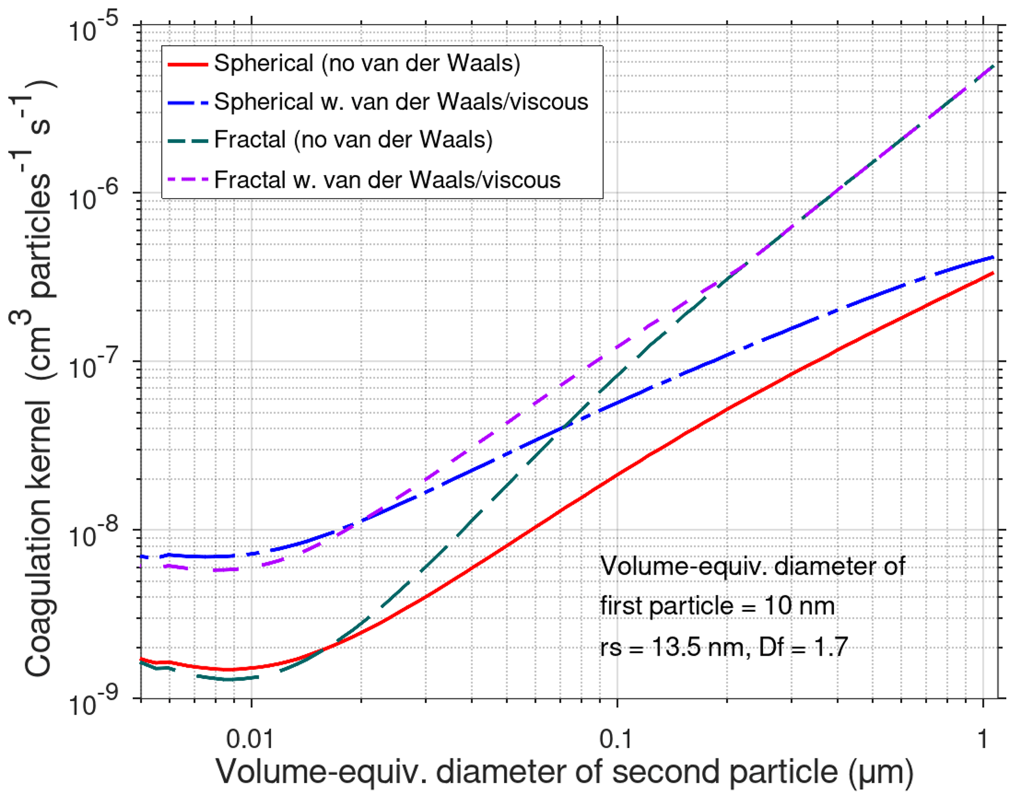
Figure 3Modelled effect of fractal geometry and van der Waals–viscous forces when the volume-equivalent diameter is 10 nm and the volume-equivalent diameter of the second particle varies from 5 to 1000 nm.
Brownian motion by far dominates the collisions of sub-micrometre particles in the atmosphere. The coagulation of particles in turbulent flow is affected by two mechanisms: spatial fluctuations of the turbulent flow and particle inertia, which cause the larger particles not to follow the flow. Since turbulent shear coagulation is only important for particles larger than several micrometres in diameter under conditions characterized by intense turbulence (Pnueli et al., 1991), its treatment is not considered in the model.
2.3.5 Dry deposition and wet scavenging of particles
Different mechanical processes contribute to the deposition of particles, mainly Brownian diffusion, interception, inertial impaction, and sedimentation. The effectiveness of the deposition process is usually described with the dry deposition velocity, Vd, which depends on the properties of the deposited aerosol particle, the characteristics of the airflow in the atmospheric surface layer and inside the thin layer of stagnant air adjacent to the surface (the so-called quasi-laminar sub-layer), and the properties of the surface. Four dry deposition schemes are included in the model: (1) Schack et al. (1985) (hereafter SPF1985), (2) Kouznetsov and Sofiev (2012) (hereafter KS2012), (3) Hussein et al. (2012) (hereafter HS2012), and (4) Zhang et al. (2001) (hereafter ZH2001). All schemes calculate size-dependent dry deposition velocities of particles.
The SPF1985 scheme considers dry deposition of particles by Brownian diffusion, interception, and gravitational settling. This parameterization is derived for deposition to completely rough surfaces based on the analysis of several field studies.
The KS2012 scheme can consider the deposition to a vegetation canopy and can be used for smooth and rough surfaces. In the KS2012 scheme, the deposition pathway is split into the aerodynamic layer between heights z1 and z0 and the in-canopy layer. Within the aerodynamic layer the Monin–Obukhov profiles of turbulence are assumed. The in-canopy layer is assumed to be well mixed and to have a regular wind speed Utop (Utop is the wind speed at top of the canopy, i.e. at height zC). The deposition in the in-canopy layer is treated as a filtration process. KS2012 defines a collection length scale to characterize the properties of rough surfaces. This collection length depends on the ratio and the effective collector size, dcol, of the canopy.
The HS2012 scheme is based on a three-layer deposition model formulation with Brownian and turbulent diffusion, turbophoresis, and gravitational settling as the main particle transport mechanisms to rough surfaces. An effective surface roughness length F+ is used to relate the roughness height to the peak-to-peak distance between the roughness elements of the surface.
The ZH2001 scheme calculates dry deposition velocities as a function of particle size and density as well as relevant meteorological variables. The parameterization is widely used in atmospheric large-scale models because it provides empirical parameters for dry deposition over different land use types.
The model user defines the roughness length, friction velocity near the surface, and other parameters specific to the dry deposition schemes in an input file.
Figure 4 shows a numerical comparison of the deposition schemes for a typical rough urban surface, representative of a street canyon using friction velocity m s−1, roughness length z0=0.4 m, and an average particle density of 1400 kg m−3. This example is chosen to illustrate the differences in the size dependence of the dry deposition velocity when all parameterizations are used with identical meteorological parameters and particle density. Effects of buildings on deposition are not considered.
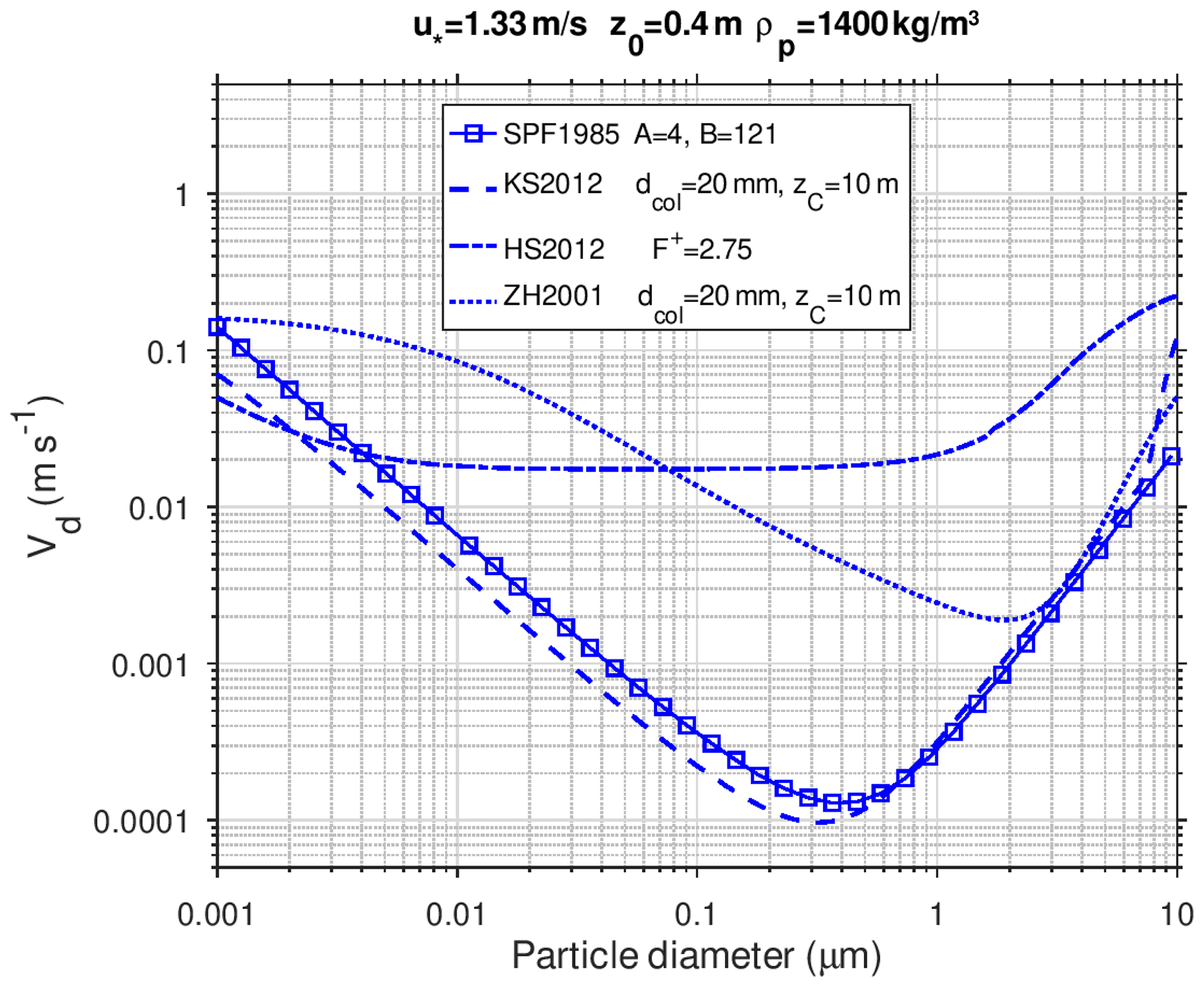
Figure 4Dry deposition of particles over a rough urban surface calculated with the SPF1985 scheme (solid line with squares), KS2012 scheme (lower dashed line), HS2012 scheme (upper dashed line), and ZH2001 scheme (dotted line) using m s−1, z0=0.4 m, and an average particle density of 1400 kg m−3. Specific parameter values are given in the legend.
Size-dependent deposition velocities calculated with the SPF1985 and KS2012 schemes agree within a factor of 2, except for large particles. Both curves have a minimum in the diameter size range 0.2–0.5 µm, while the curve from the ZH2001 scheme has a minimum at ∼2 µm. For the HS2012 scheme, an upper-limit value of the effective surface roughness length () was chosen, which is adequate for dry deposition to rough environmental surfaces, that results in higher deposition velocities for particles above 0.1 µm diameter compared to the other schemes. For particles in the size range between 0.01 and 0.5 µm the calculated deposition velocities with HS2012 are nearly independent of particle size.
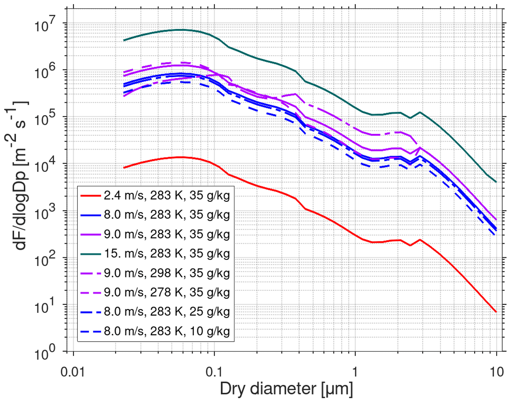
Figure 5Sea salt particle source function (size-dependent number flux, F) at different wind speed, sea surface temperature, and salinity with the parameterization by Spada et al. (2013). The effect of wind speed is shown with the green, violet, blue, and red solid lines (at SST 283 K and salinity of 35 g kg−1). The effect of SST is shown with the solid and dashed violet lines (at 9 m s−1 and salinity of 35 g kg−1). The effect of salinity is shown with the solid and dashed blue lines (at 8 m s−1 and SST 283 K).
Wet scavenging of particles is described with a simple parameterization of the scavenging rate for in-cloud removal of particles by accretion based on Pruppacher and Klett (1997). Nucleation-mode particles are not scavenged. The wet scavenging rate of particles, λwet, (s−1) is parameterized as
where fc is the volume fraction occupied by clouds, assumed to be 0.1, which is typical for the marine boundary layer. The precipitation rate P (mm h−1) can be provided in the input by the model user and may vary with time.
2.3.6 Emission of particles
Emissions of primary particles are controlled by an input file. The prescribed particle emissions can either occur at a constant rate during the entire simulation period or be time-varying as in the simulation of the Urban Case. The emitted size spectrum of particles and their chemical composition are defined by the model user.
Emissions of marine sea salt particles are calculated online using the emission parameterization from Spada et al. (2013), which combines the number flux parameterizations of Mårtensson et al. (2003), Monahan et al. (1986), and Smith et al. (1993). Sea salt particles are assumed to be composed of NaCl. A treatment of primary organic aerosol (POA) particle emissions from the ocean surface will be developed in the future. The parameterization of Spada et al. (2013) describes the size distribution of sea salt particle emissions in terms of number for the diameter size range 0.2–10.0 µm. Sea salt particle emissions in the model depend on wind speed (provided in the meteorological input), sea surface temperature (SST; user-provided value), and salinity (user-provided value). The wind speed dependence is described by the whitecap coverage relating to the 10 m wind speed and the fraction of the sea surface covered by whitecaps. Figure 5 shows the size-dependent sea salt particle flux as a function of particle size for different conditions.
2.4 Dynamic partitioning of semi-volatile inorganic gases
Several aerosol models rely on thermodynamic equilibrium principles to predict the composition and physical state of inorganic atmospheric aerosols. Examples of thermodynamic equilibrium aerosol models commonly applied in 3-D CTMs include EQUISOLV II (Jacobson, 1999), MARS (Binkowski and Shankar, 1995), ISORROPIA (Nenes et al., 1999), and AIM (Wexler and Clegg, 2002). However, in cases in which the equilibrium timescale is long compared to the residence time of particles in a given environment, the thermodynamic equilibrium is not a good approximation (Meng and Seinfeld, 1996). A dynamic partitioning approach for the formation of secondary inorganic aerosol (SIA) is therefore preferable and is expected to give results that are more realistic.
To enable dynamic partitioning of semi-volatile inorganics in the model, the APC scheme for condensation and evaporation (Sect. 2.3.2) was extended with the PNG scheme (Jacobson, 2005a). The PNG scheme involves four steps: (1) calculation of the growth of semi-volatile acidic gases by dissolution at moderate and high aerosol LWC (determined as total liquid water over all sizes), (2) calculation of the growth of semi-volatile acidic gases by condensation at low LWC, (3) calculation of the growth of non-volatile gases (such as H2SO4 when forming ammonium sulfate) at all LWC, and (4) equilibration of NH3 and pH between the gas phase and all particle size bins while conserving charge and moles.
In this implementation, the PNG scheme is coupled with the iterative equilibrium code MESA (Zaveri et al., 2005b) that calculates internal aerosol composition and the size-dependent solubility terms. Figure 6 illustrates the workflow for the coupling between the PNG scheme and the thermodynamic equilibrium module of the MOSAIC model. MESA computes aerosol phase state, temperature-dependent equilibrium coefficients, activity coefficients of electrolytes (solutes), and the water activity coefficient in all size sections for solid, liquid, and mixed-phase aerosols. MESA solves the solid–liquid equilibrium by applying a pseudo-transient continuation technique to the set of ODEs describing the precipitation reactions and dissolution reactions for each salt until the system satisfies the equilibrium or mass convergence criteria. The internal aerosol composition in MESA includes sodium (Na+), chloride (Cl−), potassium (K+), calcium (Ca2+), magnesium (Mg2+), sulfate (), NH3 ammonium(), and HNO3 nitrate () in the ionic, liquid, and/or solid phases. MESA employs the multicomponent Taylor expansion method (MTEM; Zaveri et al., 2005a) for estimating activity coefficients of electrolytes. MTEM calculates the mean activity coefficient of the electrolyte in a multicomponent solution on the basis of its values in binary solutions of all the electrolytes present in the mixture.
The PNG scheme solves the growth of particles by dissolution of semi-volatile compounds (here HNO3 and HCl) when the LWC is moderate or high (here: > 0.01 µg m−3); i.e. a liquid solution pre-exists on the particle surface. The concentration change in particle compound q (here either the dissolved, undissociated nitric acid plus the nitrate ion or the undissociated hydrochloric acid plus the chloride ion) due to dissolution in one size bin is
where accounts for the Kelvin effect and is the dimensionless effective Henry's law coefficient for the respective size bin. However, if a solid pre-exists in a particle size bin, condensation occurs and
The saturation vapour concentration (short: SVC) varies continuously over the aerosol size distribution as a function of particle composition. The size-dependent SVC and the effective Henry's law coefficient are calculated in the MOSAIC solver at the beginning of the time step. The size-dependent SVC of HNO3 and of HCl is determined by several processes (gas–ion reaction, solid–gas equilibrium, and solid–ion reactions). The minimum SVC arising in any of the processes is chosen for the calculation of the condensation term when a solid is present in a particle size bin. The gas concentration Cg,q and the total dissolved concentration are unknowns in Eq. (15).
Integration of Eq. (15a) for one size bin over a time step Δt gives (Jacobson, 2005a)
The final gas concentration of the semi-volatile acid and final particle concentration in each bin are obtained analogous to the APC scheme with the solution described in Appendix B. The solution is unconditionally stable and mole-conserving.
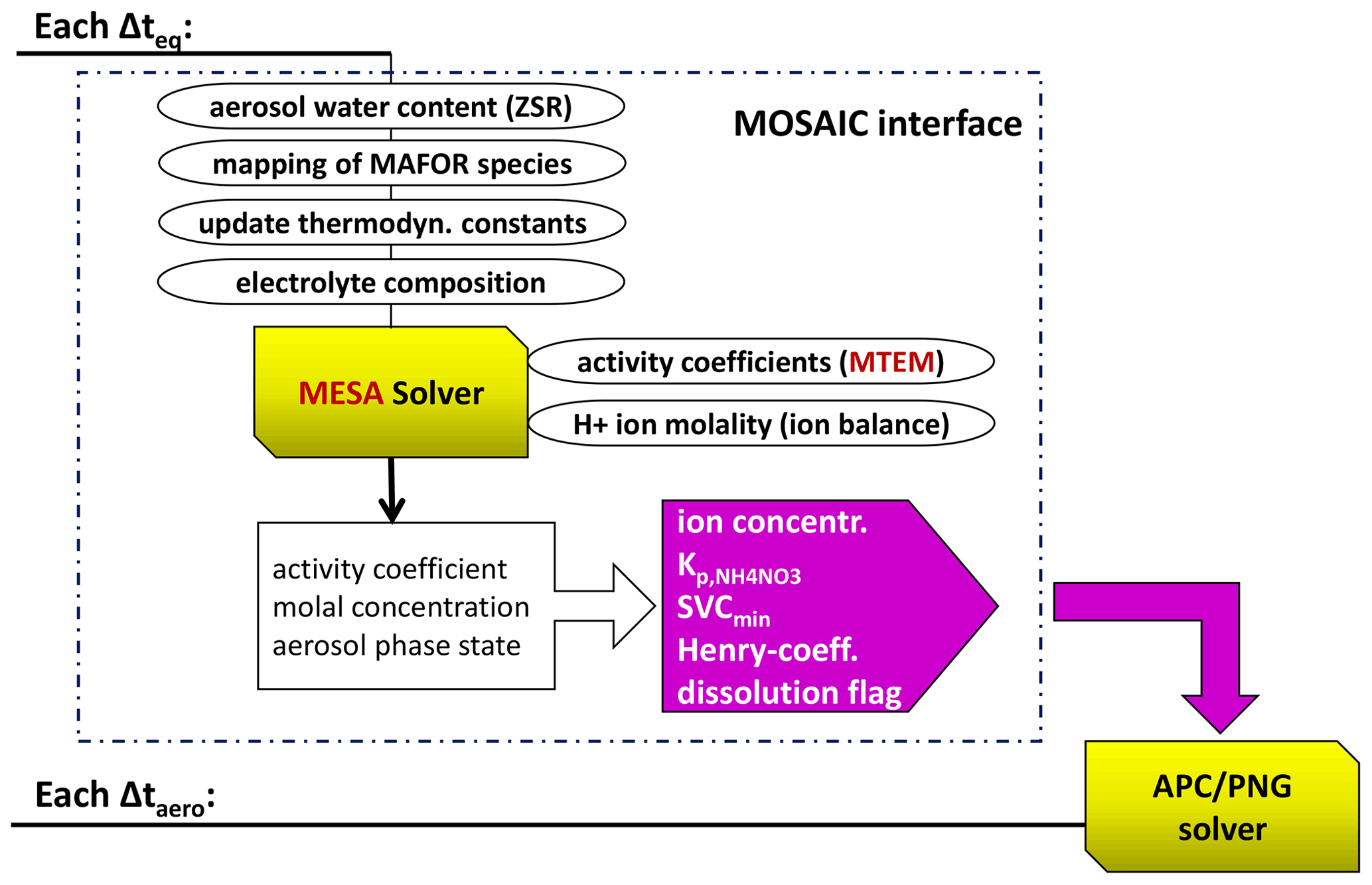
Figure 6Workflow of the dynamic partitioning of semi-volatile inorganic gases. The MOSAIC interface is called every Δteq=120 s, while the PNG solver is called every time step of the aerosol dynamic solver (Δtaero). The MOSAIC interface outputs the gas–solid equilibrium coefficient for ammonium nitrate, the minimum saturation vapour concentration (SVCmin), the effective Henry's law coefficient, the ion concentrations, and a dissolution flag (indicating if a solid is present in a size bin or not) for each size bin of the particle population.
When the LWC is below 0.01 µg m−3, the growth of nitric acid is treated as a condensation process rather than a dissolution process. The saturation vapour concentrations of HNO3 and HCl are calculated considering the gas–solid equilibrium of ammonium nitrate and the gas–solid equilibrium of ammonium chloride as described in Jacobson (2005b). The solution for the coupled ammonia–nitric acid–hydrochloric acid system is then obtained from Eq. (6) and the growth by condensation is treated in the APC solver (Sect. 2.3.2). The condensation and evaporation of low-volatility or non-volatile gases, such as H2SO4 and high-molecular-weight organics, are solved as a condensation process among all size bins independent of the aerosol LWC.
Following the growth calculation for the acidic gases, NH3 is equilibrated with all ions and solids in all size bins of the aerosol phase, conserving charge among all ions, also for those that enter the liquid solution during the dissolution and condensation process. NH3 is equilibrated with all size bins of the aerosol phase simultaneously, resulting in an exact charge balance among all ions in the solution, and conserves mass of NH3 between the gas phase and all particle size bins.
Following the ammonia calculation, an operator-split internal aerosol equilibrium calculation in the MESA solver is performed to recalculate aerosol ion, liquid, and solid composition, activity coefficients, and Henry's law coefficients, accounting for all species in solution in each size bin. In order to reduce the computational time, the liquid solution terms and composition are updated at longer time intervals than the aerosol dynamic solver time step (Δtaero). The operator-split time interval between growth and equilibrium is 115 s in the current implementation. An advantage of the PNG scheme is that it can be applied at a long time interval (several minutes) without causing oscillatory behaviour in the numerical solution (Jacobson, 2005a). Such oscillatory behaviour at a long time step was observed in an earlier dissolution solver (Jacobson, 1997b) that did not treat the condensation (dissolution) of acid and base separately.
2.5 Absorptive partitioning of organic vapours
The new concept for SOA formation in MAFOR v2.0 relies on the 2-D VBS framework introduced by Neil Donahue and co-workers (Donahue et al., 2011). This classification uses the carbon oxidation state and the saturation concentration of the pure compound to define the organic aerosol composition in a two-dimensional space. The 2-D VBS is able to represent the variety of organic aerosol components in the atmosphere and their conversion due to ageing chemistry.
A hybrid approach of condensation–evaporation (Sect. 2.3.2) and the absorptive partitioning into an organic liquid is used to treat condensation to an organic mixture considering non-ideal solution behaviour. For absorptive partitioning, the equilibrium gas-phase concentration (or saturation concentration) of the condensing organic vapour can be obtained from the following relation (Bowman et al., 1997):
where mtot,p is the total particle mass concentration, mtot,q is the total mass concentration of compound q in the particle, fom is the fraction of absorbing organic material in the aerosol, and Kom,q (m3 µg−1) is the absorption partitioning coefficient of the compound. Using the relation for the mass-based absorption partitioning, (Donahue et al., 2006), Eq. (17) can be rewritten as
with the effective saturation mass concentration (in µg m−3) of compound q:
where γom,q is the activity coefficient of the individual compound (solute) in the organic mixture (solvent). A simplifying assumption of the 2-D VBS framework is that the activity coefficient is a function of the average carbon fraction (O : C) of the organic aerosol as well as the properties of the individual organic solute. Donahue et al. (2011) give an empirical relation to estimate the activity coefficient γom,q for organic mixtures (at 300 K):
where bCO is an empirical constant for the carbon–oxygen non-ideality (), nM is the size of the solute calculated as sum of carbon and oxygen atoms, is the carbon fraction of the individual solute, and is the carbon fraction of the solvent. The activity coefficient for compound q depends exponentially on the size of the solute, while the non-ideality is driven by the differences between the carbon fraction in the solvent and the solute. The formulation of the activity coefficient neglects the role of water or other inorganics in the absorbing material. The effect of these constituents may be treatable within the 2-D VBS framework in the future.
Three classes of organic compounds are represented in the model: oxidized secondary biogenic organics, oxidized secondary aromatic organics, and primary emitted organics. Each class is divided into three volatility levels, resulting in a total of nine lumped gaseous SOA precursors. Formation of secondary organic compounds is coupled to the gas-phase chemistry of biogenic VOCs (isoprene, monoterpenes) as well as aromatic VOCs (toluene, xylene, trimethylbenzene). The lumped SOA precursors are produced in the gas-phase oxidation reactions via their molar stoichiometric yields. They can undergo oxidative ageing and/or oligomerization. Primary emitted organics can either undergo oxidative ageing or fragmentation. Figure 7 presents a scheme of SOA formation reactions in the model.

Figure 7Chemical reactions involved in SOA formation. BRO2 and ARO2 stand for all the peroxy radicals of the respective biogenic or aromatic VOCs. The molar stoichiometric yields α1, … , α5, and β1, …, β5 represents the formation yields of SOA precursors in the gas-phase reaction of biogenic and aromatic VOCs, respectively. Oligomerization and fragmentation reactions are approximated with first-order rate constants (Tsimpidi et al., 2010; Lambe et al., 2009; Carlton et al., 2010; Lim and Ziemann, 2009). The nine lumped organics are BSOV (biogenic semi-volatile compound), BLOV (biogenic low-volatility compound), BELV (biogenic extremely low-volatility compound), ASOV (aromatic semi-volatile compound), ALOV (aromatic low-volatility compound), AELV (aromatic extremely low-volatility compound), PIOV (primary intermediate-volatility compound), PSOV (primary semi-volatile compound), and PELV (primary extremely low-volatility compound).
Extremely low-volatility organic compounds (ELVOCs) may play an important role in new particle formation. Ehn et al. (2014) have demonstrated the significant formation of ELVOCs with a branching ratio of ca. 7 % in the reaction of α-pinene with ozone (O3). The compounds have been identified as highly oxygenated molecules (HOMs). Their formation is induced by one attack of ozone in the initial reaction of the monoterpene, followed by an autoxidation process involving molecular oxygen. In the model, the production of ELVOCs from monoterpenes (represented by BELV) is simplified by assuming direct formation in the reaction of the monoterpene with O3. The formation of HOMs in the reaction of aromatics with hydroxyl (OH) radicals occurs either via an autoxidation mechanism or via multi-generation OH oxidation steps (Wang et al., 2020). Again, only direct formation of ELVOCs (represented by AELV) in the initial reaction of toluene with OH radicals is implemented here. The model further assumes that BELV and AELV are the products from the oligomerization reaction of more volatile organics. It is possible to implement a more detailed treatment of the autoxidation mechanism in the future.
The implementation of the 2-D VBS framework requires a series of input parameters for each SOA precursor, namely the number of carbon atoms, number of oxygen atoms, saturation concentration C0, and enthalpy of vaporization. The user-provided C0 value (in µg m−3) of the lumped organic compound is then used to compute the saturation vapour concentration according to Eqs. (17)–(20).
2.6 Numerical solution of the aerosol dynamics
The model solves the particle number and mass concentration distribution of a multicomponent aerosol using the full stationary (fixed) sectional method. The fixed sectional method (Gelbard and Seinfeld, 1990; Tsang and Rao, 1988) is computationally efficient and advantageous when treating continuous nucleation of new particles, which is relevant for the modelling of new particle formation. The method is also convenient for the combined treatment of nucleation, emission, coagulation, and particle transport because the particle volume in one size section is always constant (Korhonen et al., 2004). This is achieved by a splitting procedure for the particle growth that determines the fraction of particles in one size bin that will grow to the next size bin. However, this splitting procedure is prone to numerical diffusion, causing a wider particle size distribution with lower peak concentrations than the accurate solution. Relevant alternative sectional methods are the full moving structure (Gelbard, 1990), the hybrid structure (Jacobson and Turco, 1995), and the moving centre structure (Jacobson, 1997a), which all eliminate the numerical diffusion arising from the splitting between size sections. The full moving structure allows the particles to grow to their exact size. However, the full moving structure causes problems if new particle formation is considered. The disadvantage of the hybrid structure is that if the particles gain or lose non-volatile material, they must be fitted back to the fixed grid. The moving centre structure allows the particle size to vary in a section within certain boundaries. It causes some numerical diffusion due to averaging of moved particles with pre-existing ones in a section.
Korhonen et al. (2004) tested different sectional structures in the simulation of the particle distribution during a new particle formation event and found that the hybrid structure was most vulnerable to numerical diffusion upon particle growth. The moving centre structure permitted fairly realistic treatment of the particle evolution (Korhonen et al., 2004). The ADCHEM model uses the moving centre structure due to its good performance when the size distribution is represented by only a few size sections (see Table 1). In the SALSA model, the moving centre structure is used for particles below 730 nm in diameter, whilst for particles larger than that, fixed size sections are used. In SALSA, the particle size spectrum is divided into three subranges based on the size. This enables variation in including or excluding microphysical aerosol processes and chemical components in simulations in each subrange based on the relevance of the process in the range. For instance, in the lowest subrange cloud processing can be neglected and particles contain only sulfate and organic matter.
Because of the advantages when simulating new particle formation, the fixed structure has been chosen for MAFOR (Karl et al., 2011). A fixed sectional grid on the diameter coordinate is used when the number of size sections can be selected by the model user. By using a high number of size sections, the numerical diffusion can be largely reduced. Karl et al. (2011) showed that in an 80 h simulation of the particle distribution in the Arctic marine boundary layer, the final number distribution for the model using 60 size bins closely agreed with the solution of the model using 120 sections. To determine the number of size bins that are necessary to accurately represent an urban particle size distribution, numerical calculations using different number of size sections were performed (Sect. S2). This test (Case 1) confirmed that the model using 60 bins performs very well in comparison to a sectional representation using 160 bins (the reference in Case 1), although slight spreading of the nucleation mode due to numerical diffusion could be noted. For lower size resolution, the discretization errors were more relevant, leading to a broader nucleation mode with peak diameter at smaller size.
In model simulations, size bins are evenly distributed on a logarithmic scale, ranging from the smallest diameter of 1 nm to the largest diameter of 10 µm. It is possible to use a different maximum diameter (in the range 1–10 µm). Typical model applications in plume dispersion simulations use 120 size sections to represent the aerosol size distribution in the size range 0.001–1.0 µm, resolving the nucleation mode at molecular level. Simulations are initiated with the particulate mass concentrations of the aerosol constituents in four aerosol modes: nucleation mode (Nuc; diameter range 1–25 nm), Aitken mode (Ait; diameter range 25–100 nm), accumulation mode (Acc; diameter range 100–1000 nm), and coarse mode (Coa; diameter range 1–10 µm). The initial mass concentrations of the lognormal modes are distributed over the size bins (Jacobson, 2005b):
where Dp,i is the particle diameter of section i, ΔDp,i the corresponding width of the section, and MA,q and σA the mass concentration of the constituent q and geometric standard deviation of the lognormal mode A, respectively. The initial number concentration in each mode is then matched by varying the geometric mean mass diameter, GMDm,A.
Due to full stationary structure, collision of particles from section k with particles from section j generates a particle which has a volume between those of two sections i and i+1 and needs to be partitioned between the two bins, as described in Appendix C. A semi-implicit method is applied to coagulation, which yields an immediate volume-conserving solution with any time step (Jacobson, 2005b). Though particle number is not exactly conserved, the error in number concentration is reduced when the number of bins to describe the size distribution is increased (Karl et al., 2011). Condensation and evaporation of vapours result in the redistribution of particles between adjacent size sections. Number concentration in section i increases when particles from section i−1 grow by condensation or particles from section i+1 shrink due to evaporation. It decreases when particles from section i change volume by condensation or evaporation of vapour.
Considering the presence of a supersaturated vapour (e.g. H2SO4), stable clusters containing a certain number of monomers, g∗, will form continuously at the rate of neutral or ion-induced nucleation (see Sect. 2.3.3), denoted by Jnuc(t). Then coagulation, heterogeneous condensation, and evaporation of vapour on and from particles of size and nucleation of g∗-mers are distinct processes. The time evolution of the particle number concentration (in m−3) and mass concentration (in µg m−3) of all aerosol constituents in section i (with , … , ) can be written as discrete general dynamic equations in Eqs. (22) and (23).
Here, f is the volume fraction of the intermediate volume of the colliding particles, δ is the Kronecker delta function, λdry (s−1) is the dry deposition rate, λdil (s−1) is the dilution rate, Nbg,i is the number concentration of background particles in the same size section, is the mass concentration of background particles of compound q in the same section, is the mass-based emission rate (), Hmix is the height of the simulation box (m), ρq is the density of compound q (kg m−3), and cv is a conversion factor to convert kilograms to micrograms. In Eq. (23), Mk is the total mass of a particle (µg) in section k (i.e. the sum of the masses of its individual components), Mj is the mass of a particle in section j, and qnuc indicates that the compound is able to nucleate (e.g. H2SO4). The first term on the RHS of Eq. (23) describes the effect of condensation and evaporation of a vapour on the total aerosol mass. The second and third terms on the RHS take into account the fact that the mass of the individual constituent increases or decreases and consequently the mass concentration distribution moves on the diameter coordinate.
The discrete equations describing the change in particle number and mass concentration with time are solved with forward finite differences. In plume dispersion simulations, MAFOR uses a time step of 0.1 s for the integration of chemistry and of the aerosol processes, which is sufficiently small when compared to the typical timescales in the range 0.5–4 s for dilution in exhaust plumes (Ketzel and Berkowicz, 2004). When simulating an air parcel along multiple-day trajectories and for chamber experiments, the time step is 5 s.
2.7 Previous applications of MAFOR in plume dispersion studies
In this section, published applications of MAFOR version 1 in plume dispersion studies and the previously developed procedure for treating the dilution term in the model are presented. An evaluation of MAFOR version 2, including the new features, against experimental data and two aerosol dynamics models is presented in Sect. 3.
The MAFOR model version 1 has been used in the European TRANSPHORM (Transport related Air Pollution and Health impacts – Integrated Methodologies for Assessing Particulate Matter) project to examine the influence of aerosol transformation processes on PN concentrations in several European cities (Karl et al., 2016; Kukkonen et al., 2016). Dry deposition and coagulation were found to be generally relevant on the neighbourhood scale, but less so in efficient dispersion conditions. Sensitivity tests with the model showed that coagulation causes removal of particles with <25 nm diameter between the roadside and ambient environment. Particle removal was further enhanced when the fractal nature of soot aggregates and the combined effect of van der Waals and viscous interactions were considered.
For the treatment of dilution of vehicular exhaust gases and particles in combination with aerosol transformation processes on the neighbourhood scale, it is practical to divide the exhaust dilution near roadways into two distinct dilution stages: the first stage (tailpipe-to-road) is characterized by traffic-generated turbulence, and in the second stage (road-to-ambient) atmospheric turbulence prevails (Zhang and Wexler, 2004). The dilution ratio in the first stage can reach up to about 1000:1 in around 1–3 s, while the dilution ratio in the second stage is commonly of the order of about 10:1 on a timescale of about 10 min. A detailed simulation of the first stage would require the use of LES to explicitly describe the plume turbulent dispersion and account for the fluctuations in the wake of the vehicles (e.g. Chan et al., 2008). However, in practical applications, the early plume phase has been mainly treated using analytic equations for the jet–plume development up to a few seconds (e.g. Vignati et al., 1999). Due to the rapid temperature decrease immediately after exhaust release, the formation of a nucleation mode has already occurred within the timescale of the first dilution stage (Rönkkö et al., 2007).
In the study of Karl et al. (2016), model simulations with MAFOR for the road-to-ambient particle evolution were initialized with particle size distribution measurements at the roadside and at an urban background station. It was assumed that emission of primary exhaust particles and nucleation processes had already occurred before the exhaust plume reached the air quality (AQ) monitoring site, located a few metres away from the street. The horizontal particle dilution parameterization was defined by a numerical power function, , where x (in m) is the distance from the roadside and U is the horizontal wind speed (m s−1) perpendicular to the road (Pohjola et al., 2007). Typical values of the dispersion parameters a and b were chosen to represent different meteorological dispersion regimes. Assuming a circular plume cross section, the particle dilution rate as a function of time is then simply .
The dispersion parameters can either be derived from dispersion models or from concentration measurements (typically of NOx) at several distances perpendicular to the road. The applied treatment of particle dilution assumes a well-mixed state within each cross-wind cross section of the plume. The simple dilution model coupled with the aerosol dynamics model has been tested and evaluated in an earlier study (Keuken et al., 2012) simulating the particle evolution downwind of a motorway under free dispersion conditions. The comparison of the modelled total PN and size distributions with measurements at different distances from the motorway gave reasonable agreement.
The model has also been applied to study the formation of particles in the exhaust of a diesel engine equipped with an oxidative after-treatment system (Pirjola et al., 2015) consisting of a dilution unit and an ageing chamber. The rapid dilution and cooling in the dilution unit were described with empirical parameterizations, wherein temperature follows the exponential curve of the Newtonian cooling and dilution is modelled by using an exponential equation for the dilution ratio, as in Lemmetty et al. (2006). These functions have been implemented in MAFOR and in AEROFOR. Modelled particle number size distributions of the two models were in good agreement with each other and with measurements after 2.7 s of exhaust dilution.
In a study of ship exhaust plumes, MAFOR was applied to determine the in-plume number size distribution and chemical composition of ultrafine particles at different distances from passenger ships (Karl et al., 2020). The dilution of aerosol particles in the ship exhaust plume was approximated using dilution parameters provided by the 3-D atmospheric dispersion model EPISODE-CityChem (Karl et al., 2019). The aerosol dynamics model was used to compute the particle number and mass distributions during the second dilution stage as a function of the distance from the ship stack along the centreline of the ship plume. Dilution in the first stage, when rapid cooling and expansion occur, was calculated with the jet plume model of Vignati et al. (1999), assuming a circular cross section of the plume. Neglecting the removal of particles by coagulation during the first-stage dilution was estimated to introduce an error of 10–15 % in the computed PN concentrations. The particle evolution in the ship plume during the second dilution stage was computed with the aerosol dynamics model considering nucleation, condensation and evaporation, coagulation of particles, dry deposition of particles, gas-phase chemistry within the plume, and mixing of the air parcel with gases and particles from the background. Modelled PN concentrations agreed within 50 % with measured PN concentrations when a peak in the signal was detected that related to the ship passage.
Recently, the MAFOR model has been utilized to investigate the particle number concentrations induced by aviation emissions in the surrounding communities of Zurich airport (Zhang et al., 2020). The offline coupling between the atmospheric dispersion model and MAFOR was achieved through the plume dilution curve, which was approximated by fitting a power-law function using the dispersion results and then adopted by MAFOR for the aerosol dynamics calculations. The plume dilution curve was analysed based on the centreline concentration of the plume. The particle evolution in the aviation exhaust was calculated with the aerosol dynamics code using the obtained dilution curve in conjunction with meteorological data (humidity, temperature, precipitation, and wind speed) and the background PN concentration. Kinetic nucleation of H2SO4, condensation and evaporation, coagulation, deposition, and mixing of the air parcel with the background particles were considered in the model simulations. The results suggested that particles between 10 and 30 nm contributed significantly to the particle number concentration. The predicted PN concentrations were within a factor of 2 of the measurements.
3.1 Experimental data for the Urban Case in Helsinki, 2010
The Urban Case scenario for the evaluation of the MAFOR model version 2 was developed as a plume dispersion study inside a half-open street canyon, where emissions from vehicular traffic and dilution with background air are the key processes in modifying PN concentrations and size distributions. Mobile and stationary measurements during a street canyon campaign (Pirjola et al., 2012) in winter 2010 (November–December 2010) in Helsinki, Finland, performed as part of the Finnish national research programme MMEA (Measurement, Monitoring and Environmental Assessment, 2010–2014), were used to construct the Urban Case scenario. Measurements with the mobile laboratory van, called Sniffer, were obtained while driving back and forth on the main street Mannerheimintie (MA) and on the side streets. Stationary measurements were performed at the sidewalks and inner courts. MA passes through the city of Helsinki in the northwestern direction. There are four vehicular traffic lanes in the considered street segment (two in each direction), and in addition, there are two tramway tracks in the middle of the street. The mean traffic flow in the busy sections of MA is about 40 000 vehicles per workday, and the fraction of heavy-duty vehicles has been estimated to be 10 %.
For the Urban Case, measurements on 13 December 2010 in the microenvironment M2 (as defined in Pirjola et al., 2012; see Fig. 8a), during the afternoon traffic rush hour between 17:00 and 18:00 local time, were selected. The length of this street canyon is 230 m. In M2, the buildings downwind of the main street are oriented perpendicular to MA, and the distance between the buildings is ∼22 m (Fig. 8b). On the other side of the street, buildings are parallel to MA. The buildings are ∼21 m tall and the width of the canyon is 38 m, leading to an aspect ratio of 0.55. Although the aspect ratio is relatively shallow and MA is a half-open environment at the place of measurements, it can be considered a street canyon due to the large traffic intensity (Vardoulakis et al., 2003).
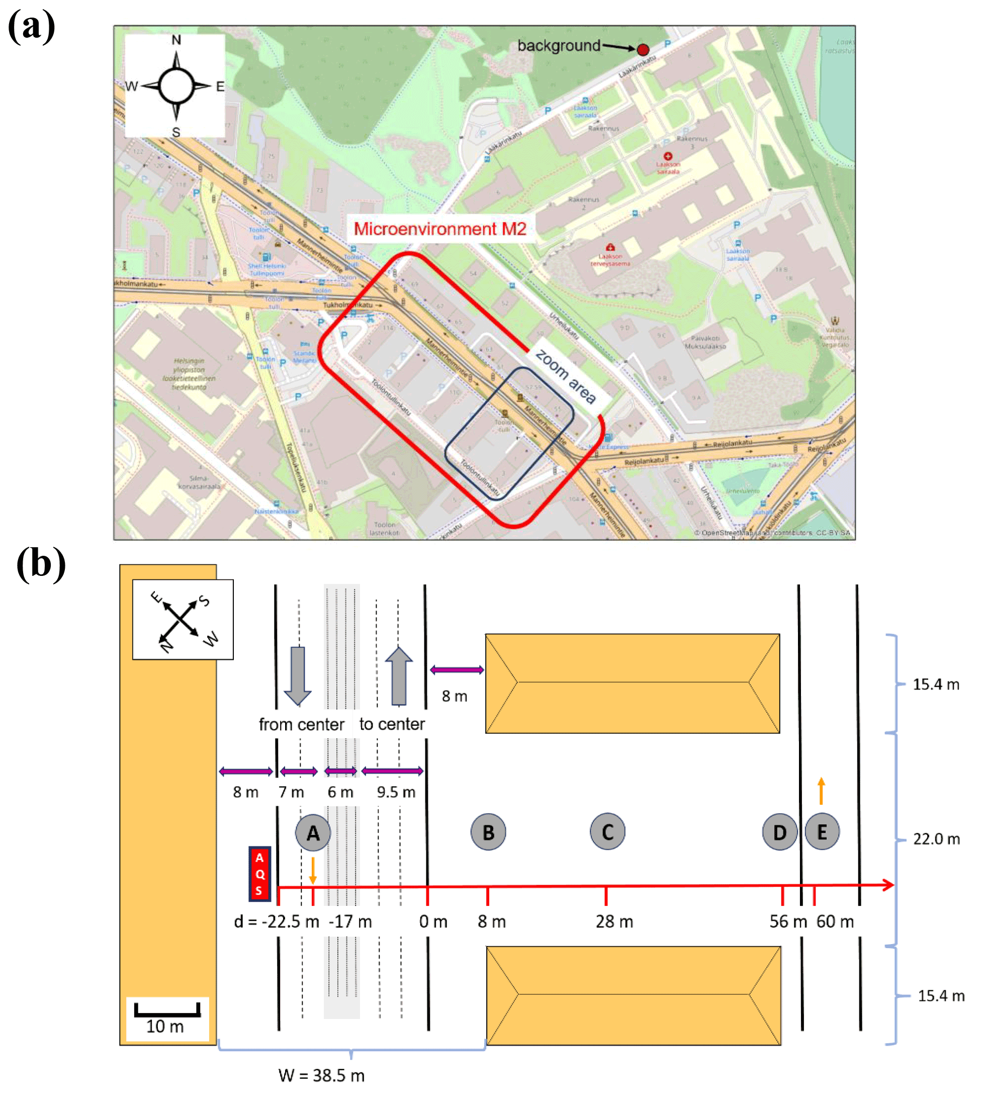
Figure 8Urban Case microenvironment M2: (a) map showing microenvironment M2, the street canyon zoom area, and the background measurement location. © OpenStreetMap contributors 2021. Distributed under the Open Data Commons Open Database License (ODbL) v1.0 (see http://www.openstreetmap.org/, last access: 14 June 2021). (b) The horizontal geometries and Sniffer measurement locations in the M2 zoom area. The red arrow shows the distance d from curbside in metres (m).
Measurements with Sniffer for dispersion studies in M2 were taken during the driving times on the second lane (outwards from the centre of Helsinki, A), during the standing times (5–10 min) downwind of MA in the space between the buildings (B, C, and D), and during the driving times on the side street (E, towards the city centre) shown in Fig. 8b. Monitoring with Sniffer included measurements of particles (particle number concentration, size distribution, particulate matter – PM2.5, and BC, as well as gases – NO, NO2, and NOx; see details of the instruments in Pirjola et al., 2012). A weather station on the roof of the van at a height of 2.9 m above ground level provided measurements of the temperature and relative humidity as well as wind speed and direction. A GPS device saved the van's speed and location. Background concentrations of particles were measured by Sniffer at Lääkärinkatu; 300 m north from M2; additionally, background air concentrations of O3, NO, and NO2 were monitored at the nearby urban background site Kallio-2 (60∘11'14.85” N, 24∘57'02.04” E). Measurements of NO, NO2, PM2.5, PM10, and BC from an air quality monitoring station (AQS) operated by the Helsinki Region Environmental Service Authority (HSY), located on the pavement of M2 (60∘11'24.51” N, 24∘54'56.81” E) (Fig. 8b), were also available.
Hourly meteorological data were estimated in this study using the meteorological preprocessor MPP-FMI (Karppinen et al., 2000). The MPP-FMI results for the selected day are based on meteorological measurements at Helsinki Vantaa airport (60.3267∘ N; 24.95675∘ E), a site which has been found to be meteorologically representative for the whole of the Helsinki Metropolitan Area. Data from MPP-FMI include the parameters defining the atmospheric stability, in addition to wind data. However, the meteorological data measured at Sniffer during the standing times in M2 were used whenever possible, as they better represented the local conditions in the street canyon. The dispersion situation for the Urban Case scenario is evaluated at Sniffer inlet height for particles, i.e. at a height of 2.4 m above the ground level.
3.2 Configuration of the simulation
In the Lagrangian air parcel simulation we assume that the initial height of the air parcel volume corresponds to the situation in which vehicular exhaust gases and particles have been diluted at a timescale of less than 0.5 s after release from the tailpipe (Pohjola et al., 2007), and the process of initial nucleation in the exhaust has been finalized. The initial air parcel height was assumed to be 0.80 m (Pohjola et al., 2007). As in previous plume dispersion studies for exhaust dilution near roadways (see Sect. 2.7), a two-stage dilution process was applied for the Urban Case scenario. The initial air parcel (sub-scale box in Fig. 9) is initialized with a concentration of particles and gases in the background air. In the first dilution stage, the dispersion of the plume and the growth of the (diluted) exhaust plume are calculated with the jet plume model of Vignati et al. (1999), which takes into account the turbulence generated by traffic, the atmospheric turbulence, and the entrainment of fresh air due to the jet effect of the exhaust gas. In the second dilution stage, when the air parcel reaches the curbside and is further transported to the ambient environment, atmospheric turbulence dominates the plume dispersion. Growth of the air parcel and dilution parameters are calculated with a line source dispersion model that considers the geometry of the street canyon.
The combination of the dispersion model and the aerosol process models was straightforward: the jet plume model and the street canyon dispersion model provided the required parameters for the dilution function of the Lagrangian air parcel, while the aerosol process models then allowed analysing the aerosol transformation within the temporally expanding volume of the plume. Figure 9 illustrates the coupling of the plume dispersion models with the aerosol dynamics models. The dilution of particles in the moving air parcel is divided into two regimes, i.e. the first between the sub-scale box from emission source to curbside and the second between curbside and the ambient environment (street environment box). The change in particle number concentration in a size section due to dilution with background air during the first stage is expressed by
During the second stage, it is expressed by
The dilution ratio DR in the vehicle exhaust plumes increases approximately linearly with time during the first seconds of the dilution. Details on the calculation of the plume height as a function of the air parcel transport time and the dilution functions are given in Appendix E. The two dilution functions were implemented in MAFOR and the other Lagrangian-type aerosol process models that were used in the comparison for the Urban Case scenario. The dispersion situation in the street canyon was first evaluated using the simplified street canyon model (SSCM), a component of the urban dispersion model EPISODE-CityChem (Karl et al., 2019). This street canyon model follows the Operational Street Pollution Model (OSPM; Berkowicz et al., 1997) in most respects but simplifies the geometry of the street canyon. Then the dilution parameters for the second stage were derived from the simulated concentrations obtained from the street canyon model using line source emissions of total PN in both directions of the street.
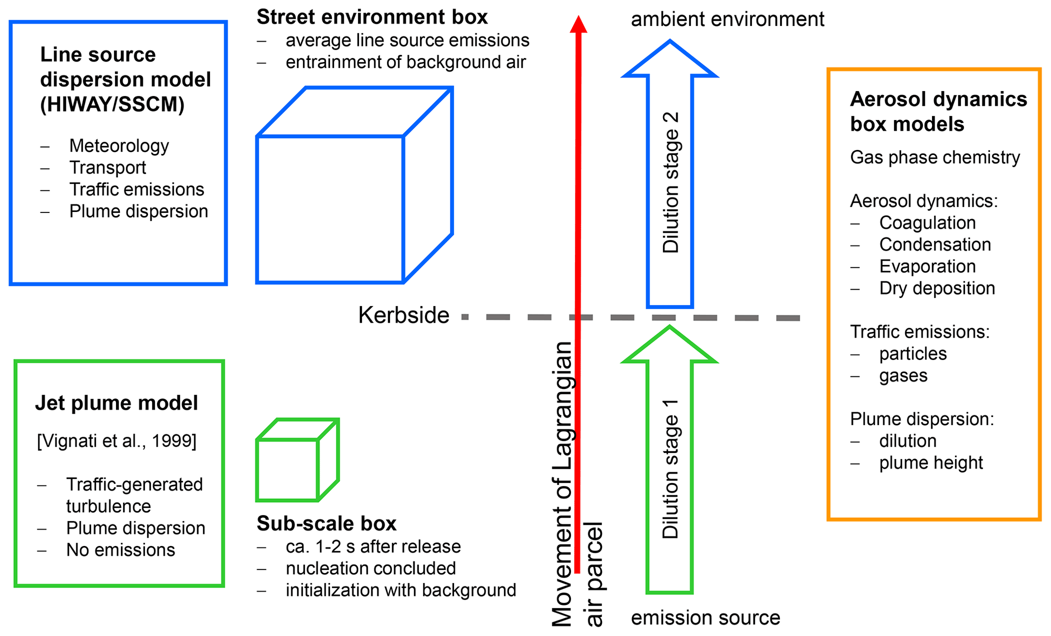
In the Lagrangian simulation, a continuous flux of vehicular emissions to the moving air parcel occurs during the times when the air parcel is transported over the lanes. The air parcel is released at m (d is the distance from curbside) and transported over the street (with the street geometry in Fig. 8b). All gaseous and particulate constituents of the air parcel are diluted during the transport, with the rate of dilution changing at curbside (d=0 m). The air parcel receives emissions while passing over the two lanes in the outwards direction, is only diluted while passing over the tram tracks, and then again receives emissions while passing over the three lanes in the direction of the city. After passing d=0 m, the air parcel is freely diluted, with no influence from buildings and ground surfaces (smooth terrain assumption).
The composition of the air parcel was initialized with particle size distribution data from Sniffer measurements in the background air, 300 m north of M2 (Fig. 8a). The chemical composition of the initial aerosol was based on the urban background aerosol described in Pohjola et al., 2007 (Table 2 therein). Table 4 summarizes the meteorological input and initial conditions for the Urban Case scenario.
Pohjola et al. (2007)Pohjola et al. (2007)Table 4Overview of meteorological input and initial conditions for the Urban Case.
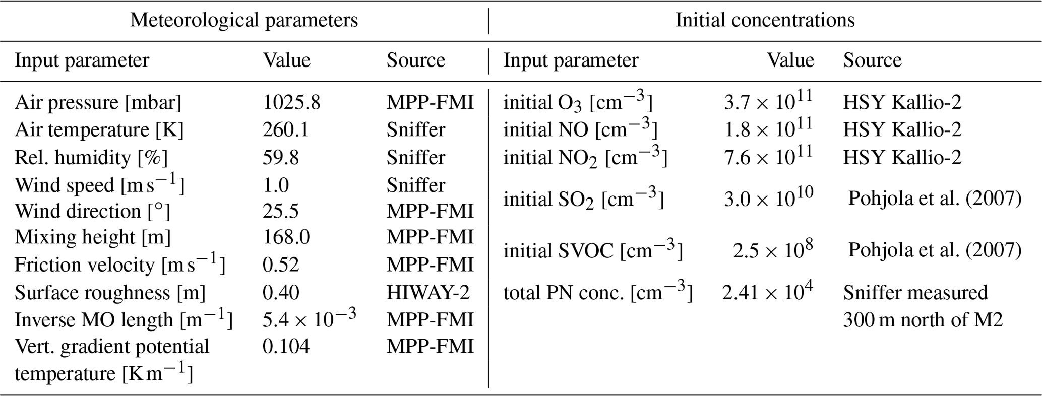
Emission factors of gases and particulates for the Urban Case were adopted from Kurppa et al. (2020; Table 3 therein). Kurppa et al. (2020) applied a particle number emission factor of EF per kilogram of fuel. Fuel consumption per vehicle (veh) of 9.8 L per 100 km is assumed here for conversion of emission factors in particle number per kilogram of fuel to units of . From this we obtain a particle emission factor of 4.14 × 10¹⁴ . This emission factor is 34 % lower than the estimate from Gidhagen et al. (2003) of 6.23 × 10¹⁴ , which was used in the model simulations of the LIPIKA campaign (Pohjola et al., 2007). Emissions of total particle numbers were distributed over the particle size spectrum by utilizing the number size distribution when Sniffer was driving on Mannerheimintie to the north so that the modelled size distribution after 5.5 m of distance from the start (on the middle of lane 2; m) matched the measured size distribution on lane 2.
Exhaust particles were assumed to be composed of organic carbon (OC) and BC with constant modal OC-to-BC ratios – nucleation mode: 100:0, Aitken mode: 80:20, accumulation mode 1 (Acc1): 40:60, accumulation mode 2 (Acc2): 60:40, as in Karl et al. (2016). The emission factors for vehicle exhaust gases EFNO, EF, EF, and EFSVOC were 4.94 × 10⁻⁴, 1.39 × 10⁻⁴, 1.0 × 10⁻⁷, and 3.9 × 10⁻⁷ , respectively (SVOC is the sum of semi-volatile organic vapours), adopted from Kurppa et al. (2020). The emission factors for the two line sources were then weighted by the vehicle count in each direction. Traffic flow was 1462 veh h−1 in the outward direction and 1085 veh h−1 in the city direction (Pirjola et al., 2012). Emissions of particles and gases in the outward direction were shared equally between the two lanes and the emissions toward the city were shared equally between the lanes in this direction. To calculate the particle emission rates () and gas emission rates (), the emission factors were divided by the width of the lanes to one direction and by the air parcel box height (plume height), assuming the air in the box is well mixed. The plume height, dilution rate, and emission rate of exhaust particles during the Urban Case simulation are plotted in Fig. E1.
3.3 Comparison with other aerosol models
Results from simulations of the Urban Case scenario with MAFOR were compared to results from two other aerosol dynamics models, AEROFOR and SALSA. Processes included in the simulation of the Urban Case for the respective aerosol process models are summarized in Table 5. MAFOR, AEROFOR, and SALSA consider the condensation of H2SO4 and organic vapours emitted from the vehicles, in addition to Brownian coagulation and dry deposition. The dilution of particles and gases according to Eqs. (24)–(25) was implemented in AEROFOR and SALSA, ensuring that the same dilution schemes were applied in all models. The three sectional aerosol dynamics models used 120 bins for the diameter range between 1 and 1000 nm, a model time step of 0.01 s for the aerosol dynamics, and a time step of 0.5 s for changes in the dilution rate. The model evaluation was done without inclusion of sulfuric acid–water nucleation. A preliminary run with MAFOR showed that freshly nucleated particles formed by the atmospheric nucleation of H2SO4 emitted from the vehicles, based on nucleation rates using the Määttänen et al. (2018a) parameterization, did not grow beyond a diameter of 2 nm in size.
Hussein et al. (2012)Schack et al. (1985)Zhang et al. (2001)Table 5Processes and employed parameterizations in each of the aerosol process models.
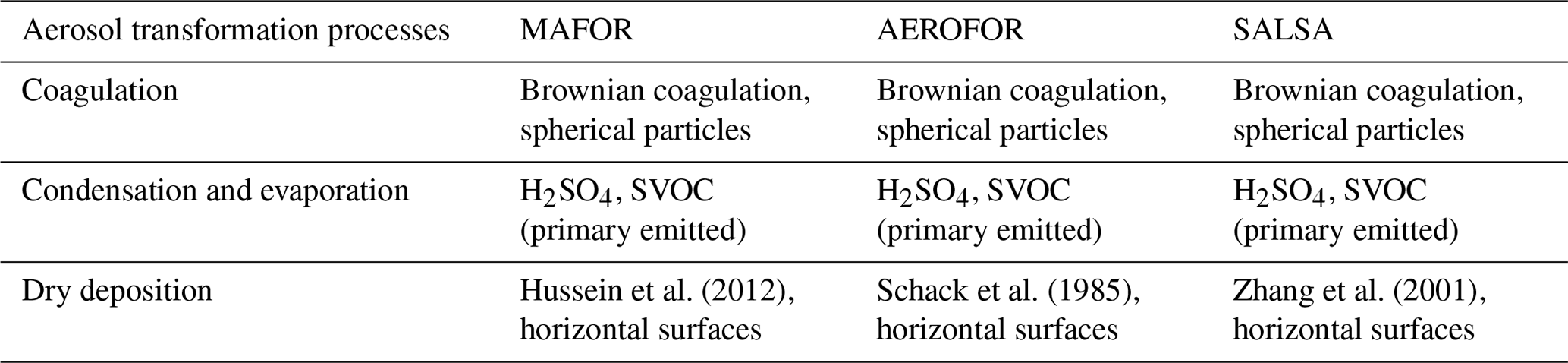
Emissions of particles were inserted differently in the models. In AEROFOR and SALSA particle emissions were distributed over the respective size sections, while in MAFOR the emitted particles as a function of size were fitted with a lognormal distribution and attributed to four modes in terms of mass and modal composition (see Eq. 21). SVOC emissions were treated slightly differently in the models: in AEROFOR they were represented by one compound with properties of adipic acid, in SALSA as semi-volatile organic carbon (Kurppa et al., 2019), and in MAFOR they were split with half to PIOV (intermediate volatility; C0=1.0 µg m−3 at 298 K) and half to PSOV (semi-volatile; C0=0.01 µg m−3 at 298 K).
LNMOM-DC treats simultaneous coagulation and dispersion from a continuous emission source (Anand and Mayya, 2015; Sarkar et al., 2020). With respect to the coagulation–dispersion system, the parameterization scheme for near-source aerosol dynamics was used as a reference for the relevance of coagulation in the Urban Case simulation.
4.1 Model evaluation against experimental data
4.1.1 Comparison with other aerosol dynamics models and experimental data
The model performance of MAFOR version 2 was evaluated in terms of total particle number, number size distributions, total particulate matter, and composition (only BC) by comparison against experimental data and against results from two other aerosol dynamics models in an urban environment. Model runs for the Urban Case were performed with the three aerosol dynamics under identical conditions for plume dispersion using the same configuration in the models to the extent that this was possible (Sect. 3.3). The focus of the model evaluation is on the analysis of aerosol processes that are relevant in urban environments. Experimental data on particle number and mass concentrations from observations within the street canyon M2, obtained with the Sniffer mobile lab, were used for the comparison. Statistical performance indicators for the model–observation (M–O) comparison were: index of agreement (IOA), coefficient of efficiency (COE), and the mean absolute error (MAE). The definitions of these indicators are given in Appendix F. In short, IOA is a refined index (Willmott et al., 2012) that spans values between −1 and +1 with values close to 1.0 representing better model performance. A COE value of 1.0 indicates perfect agreement, while negative values of COE indicate that the model predicts the observed variation less effectively than the mean of the observations. The M–O comparison was based on a four-point dataset obtained at the locations A, B, C, and D (see Fig. 8b) where Sniffer was positioned during the measurement campaign. Location E was excluded from the analysis because it appears that the measurements at E were affected by emissions from outside the street canyon. The statistics were prepared for each of the models. Note that model results are instantaneous concentrations, whereas experimental data represent an average over a longer time period (typically 5–10 min). Therefore, it is worth noticing that the large variation in the traffic situations, especially while Sniffer was driving on the main street and on the side street, might have affected the experimental results.
First, the predicted total PN concentrations from the three aerosol dynamics models were compared against measurements by SMPS (scanning mobility particle sizer; combined with a nano-SMPS). Figure 10 shows the modelled time series of total PN from the three models and the measured total PN (including 1σ standard deviation) as a function of downwind distance, which is the distance from the edge of the road ( m; Fig. 8), i.e. the starting point of the simulation, in the downwind direction. All models matched the total PN concentration at street level and the reduction of PN concentrations with increasing distance from the street, as the vehicular exhaust plume is diluted in the open space between the buildings. The total PN curve predicted by SALSA deviates from the other models after curbside; in 120 m of downwind distance total PN remains 52 % higher than in the other models. The statistical evaluation revealed that AEROFOR and MAFOR were in slightly better agreement with the measurement data than SALSA, although the differences in performance are small. Measured and modelled concentration values at the four measurement points, together with the statistical performance parameters for all models, are displayed in Table 6.
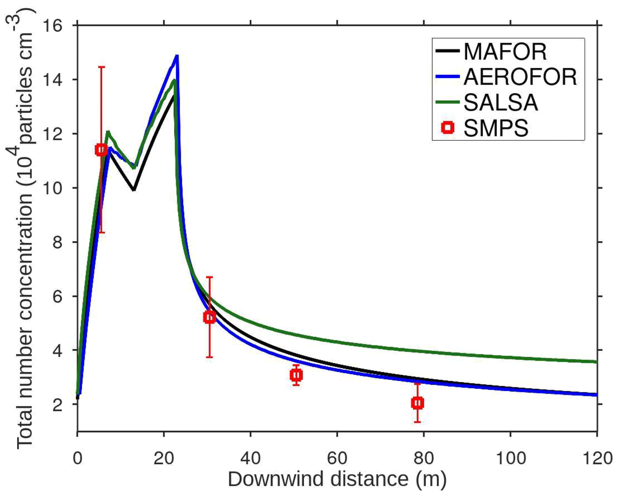
Figure 10Comparison of total particle number concentrations as a function of downwind distance in the Urban Case scenario. Model results from the aerosol dynamics models MAFOR, AEROFOR, and SALSA. Measurement data from SMPS at points A, B, C, and D (error bars indicate 1σ standard deviation).
Table 6Comparison of modelled total number concentration from different aerosol dynamics models and measured data together with statistical indicators. Standard deviations of measurements are given in round brackets.
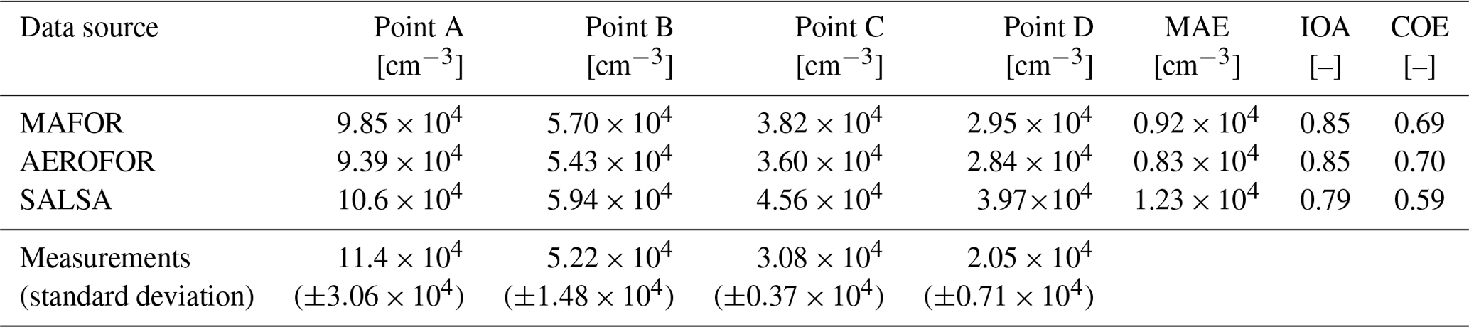
Next, the modelled and measured particle number size distributions were compared at the four point locations A, B, C, and D (Fig. 11). Modelled number size distributions at point A, at street level, to a large extent reflect how the vehicular particle emissions were distributed over the relevant size range. SALSA and AEROFOR, both using a bin-wise distribution of emitted particles, capture the measured size distribution at point A, especially in the size range <20 nm in diameter, better than MAFOR using a mode-wise distribution. Clearly, the bin-wise distribution allows for a more accurate representation of particle emissions. However, the particle size distribution of SALSA does not match the peak of the measured size distribution at 15–30 nm, in contrast to MAFOR and AEROFOR. At the second location, point B, at 8 m of distance from the street, particle concentrations have been strongly diluted (Fig. 10) and the modelled distributions are now closer to each other and the measured distribution. At points C and D, both modelled size distributions from AEROFOR and SALSA apparently overestimate number concentrations in the size range 7–20 nm compared to the measurements, indicating that the small particles are not removed efficiently enough. Number concentrations of larger particles (>100 nm in size) at greater downwind distance (points C and D) show a large variability that was not captured by the models. The possibility that sources of large particles from outside the street canyon contributed to the number size distribution measured at points C and D cannot be excluded.
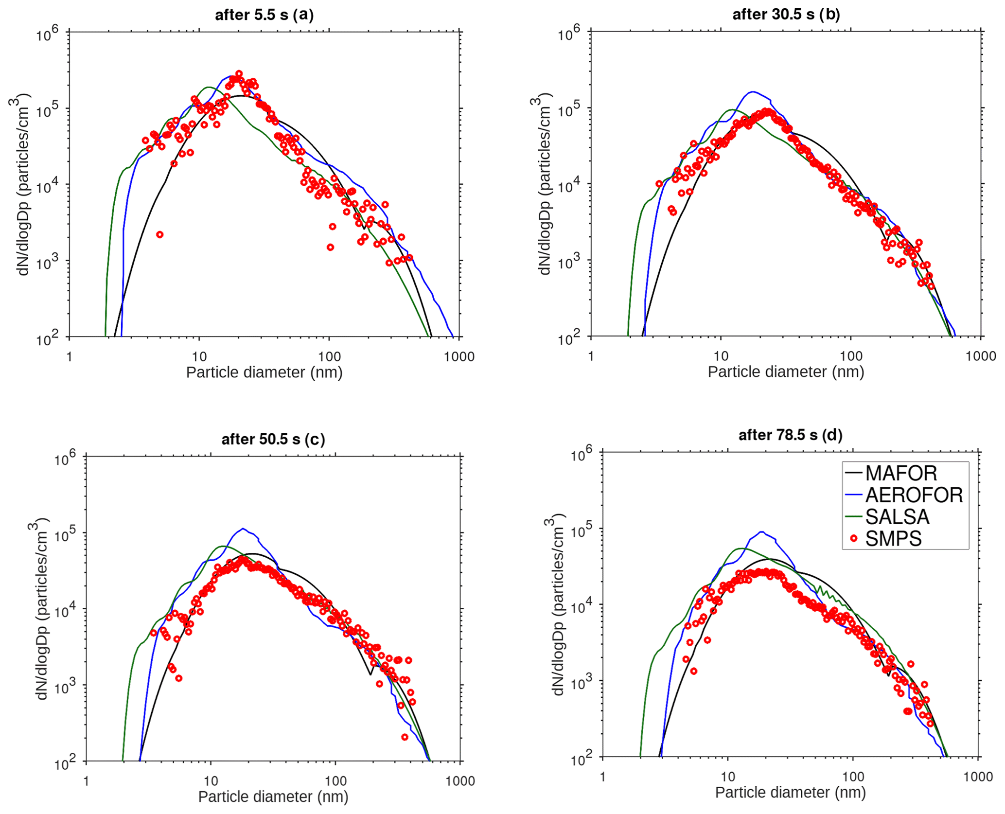
Figure 11Comparison of particle number size distributions in the Urban Case scenario. Modelled size distributions from the aerosol dynamics models MAFOR, AEROFOR, and SALSA and measured size distributions from SMPS are shown at location points A, B, C, and D.
Table 7Statistical performance indicators for the comparison of modelled and measured number size distributions for each location point A, B, C, and D as well as the average performance (mean IOA and mean COE). MAE is given in particles cm−3.
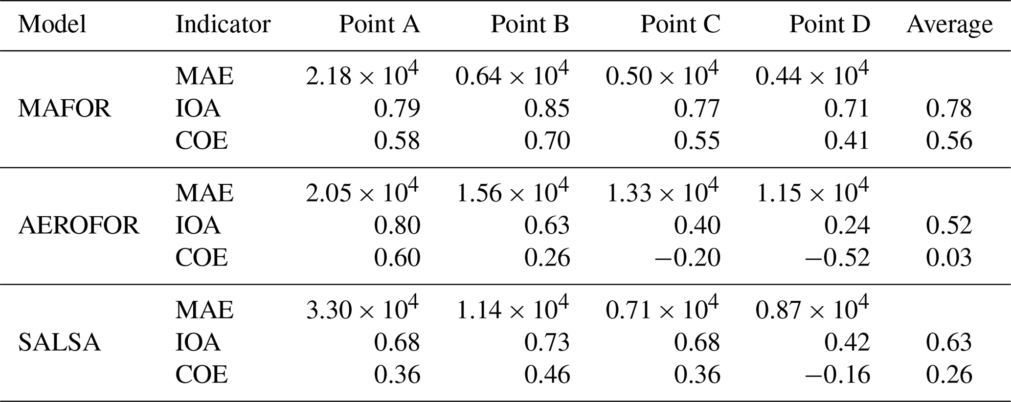
The measured size distribution from SMPS spans the size range of 3–420 nm in diameter with a size resolution of 138 bins. For the M–O comparison, the modelled size distributions () were synchronized to the size resolution of the measured size distribution by linear interpolation. The statistical comparison of size distribution was evaluated separately at points A, B, C, and D. Results of the performance evaluation at the four points and the average performance are presented in Table 7. It turns out that MAFOR and AEROFOR performed better in the prediction of the size distribution at street level (point A) compared to SALSA. However, the deviation between modelled size distributions from AEROFOR and the measured ones becomes larger with increasing downwind distance. All models show the weakest predictive capability at point D. Overall modelled size distributions from MAFOR are in good agreement with the measured distributions (IOA range: 0.71–0.85; mean IOA: 0.78), and the model has the smallest MAE at points B–D. MAFOR best reproduced the development of the number size distribution with increasing distance from the road edge. The weaker performance of SALSA (mean IOA: 0.63) is mainly due to the lower peak diameter of the modelled size distributions compared to the measured size distributions (Fig. 11).
Modelled and measured total particle mass and BC concentrations were also compared. Modelled PM1 (particles with <1µm in diameter) from MAFOR and SALSA was compared against measurement data on PM1 from an ELPI (electrical low-pressure impactor), assuming particle density of 1000 kg m−3. MAFOR outputs mass concentrations and mass size distributions, while SALSA outputs volume distributions of total mass and components. From AEROFOR no output of particle mass or volume is available. Comparison of PM1 from ELPI to PM2.5 measured with DustTrak at Sniffer indicates that the mass of supermicron particles contributed little to PM2.5 (Fig. 12a). The DustTrak measurements had large relative uncertainties, which can be attributed to short-term variations caused by passing exhaust plumes at street level, for instance from heavy-duty vehicles, or from other sources outside the street canyon. Measurements of BC with an Aethalometer similarly show high uncertainty at street level and at point E (Fig. 12b).
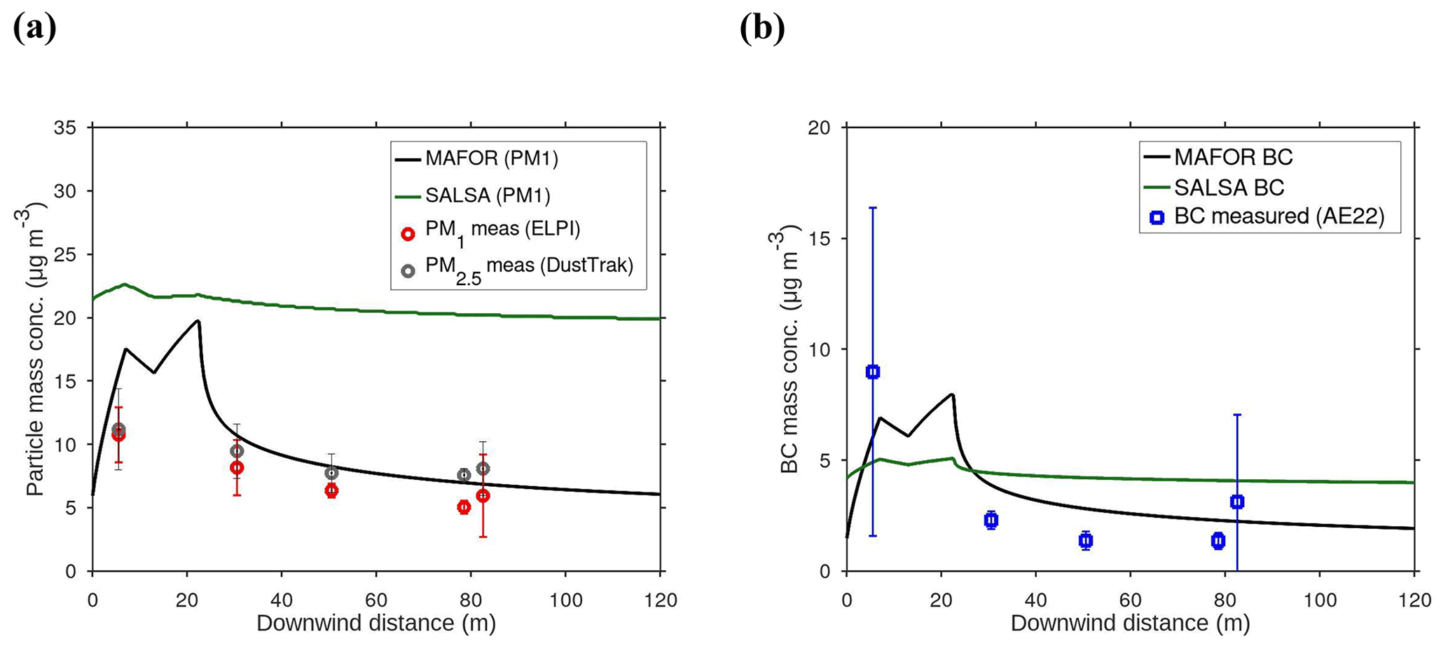
Figure 12Comparison of total particle mass and black carbon concentrations in the Urban Case simulation: (a) modelled particulate matter (PM1) from MAFOR and SALSA together with measured PM1 from ELPI (assuming particle density of 1000 kg m−3) and PM2.5 from DustTrak (error bars represent 1σ standard deviation); (b) modelled BC from MAFOR and SALSA together with measured BC with an Aethalometer (AE22, Magee Scientific; error bars represent 1σ standard deviation). Measurement data were obtained with the mobile lab Sniffer at location points A–E. Note that point E was excluded from the M–O comparison.
Modelled PM1 from SALSA considerably overestimated measured PM1. Modelled PM1 from MAFOR was closer to the measurements, although modelled PM1 at point A was 45 % higher than measured PM1 (Fig. 12a). The statistical indicators show that MAFOR (MAE = 2.29 µg m−3, IOA = 0.26, COE = −0.48) and SALSA (MAE = 13.0 µg m−3, IOA = −0.76, COE = −7.41) both have a weak performance in predicting the variation of the observations. However, the absolute error of MAFOR model results is still acceptable, and the IOA indicates better agreement with observations than the SALSA model.
Measurements of black carbon concentrations show a steeper decline between points A and D than the modelled BC concentrations from the two aerosol process models (Fig. 12b). MAFOR overestimated measured BC concentrations between points B and D but captured the decreasing trend in measured BC. The statistical evaluation shows that MAFOR (MAE = 1.72 µg m−3, IOA = 0.69, COE = 0.37) performs slightly better than SALSA (MAE = 2.94 µg m−3, IOA = 0.46, COE = −0.07) in predicting variation of observed BC. Due to the large variation in the uncertainty bars of measured BC, results from the M–O comparison for BC should be regarded with caution.
The comparison of gas-phase concentrations of condensing vapours was of particular interest to analyse discrepancies in the magnitude of condensation and evaporation between the models. In the absence of measurements of these compounds, only the model results were compared with each other. Figure 13 shows the comparison of modelled gas-phase concentrations of sulfuric acid and semi-volatile organics (sum of condensable organic vapours) calculated by the three aerosol dynamics models. While modelled peak concentrations of condensable vapours at street level were very similar among the models, differences can be noted at greater downwind distance. For H2SO4, the maximum deviation of a single model from the model mean was ±3.0 % at peak concentration but ±96 % at 100 m of distance from the road edge. For SVOCs, the maximum deviation was ±2.4 % at peak concentration and ±32 % at 100 m of distance.
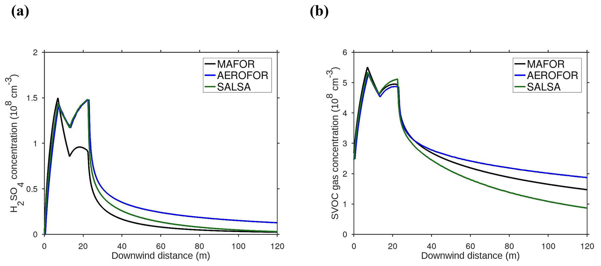
Figure 13Comparison of modelled gas-phase concentrations as a function of downwind distance in the Urban Case simulation: (a) sulfuric acid and (b) sum of semi-volatile organics (here SVOCs for short).
Modelled H2SO4 from MAFOR shows a notably lower second peak (at around 18 m downwind distance) than the other two models. This appears to be a sign of faster condensation of H2SO4 to the particle population in the simulation with MAFOR compared to the other models. The applied vapour pressure and accommodation coefficient of H2SO4 were not identical in the different aerosol models. The relevance of condensation in MAFOR simulations will be discussed in more detail in Sect. 4.1.3.
4.1.2 Importance of aerosol processes
The importance of aerosol processes was evaluated for total PN concentrations by comparing the model runs including all processes to model runs excluding one of the aerosol processes, i.e. either condensation and evaporation, dry deposition, or coagulation, and excluding all aerosol processes (dilution only). The evaluation was based on the change in total PN concentration between point A and point D relative to the PN concentration at point A:
The relative contribution of dilution was calculated as RCdilution(%)=ΔPNPNall×100, whereas the relative contribution RCproc(%) of aerosol processes was defined as
Table 8 summarizes the results of the process evaluation. Dilution dominated the change in total PN between street level and neighbourhood scale in the model runs, with a relative contribution in the range 86 %–96 %. Although the same dilution function was implemented in the models, PN change in simulations with AEROFOR was more strongly controlled by dilution than in simulations with the other models. In all aerosol dynamics models, dry deposition was the most important aerosol process, while coagulation played a minor role.
Dry deposition caused a reduction in the total PN concentration (ΔPNall−ΔPNdeposition) by 9 %, 3 %, and 6 % in model runs with MAFOR, AEROFOR, and SALSA, respectively. Differences in the relative contribution of deposition in the models are most probably due to the different schemes for dry deposition in the models (Table 5). To assess the differences in the model results due to the application of different deposition schemes, additional model runs including all processes were performed with the MAFOR model, first using the deposition scheme in AEROFOR (SPF1985) and second the deposition scheme in SALSA (ZH2001). The comparison of the final particle size distribution at point D is shown in Fig. E2, obtained from MAFOR runs with different dry deposition parameterizations. The HU2012 deposition scheme that was used in the reference run with MAFOR was more efficient in removing particles >10 nm in diameter than the other two deposition schemes. However, differences between using either the scheme SPF1985 or ZH2001 were negligible, which implies that the application of different dry deposition parameterizations was not the main reason for differences of the predicted particle size distributions.
Table 8Importance of dilution and aerosol processes in the Urban Case scenario: relative changes in total PN concentrations between points A and D (ΔPN) and relative contribution (RC) of dilution and aerosol processes.
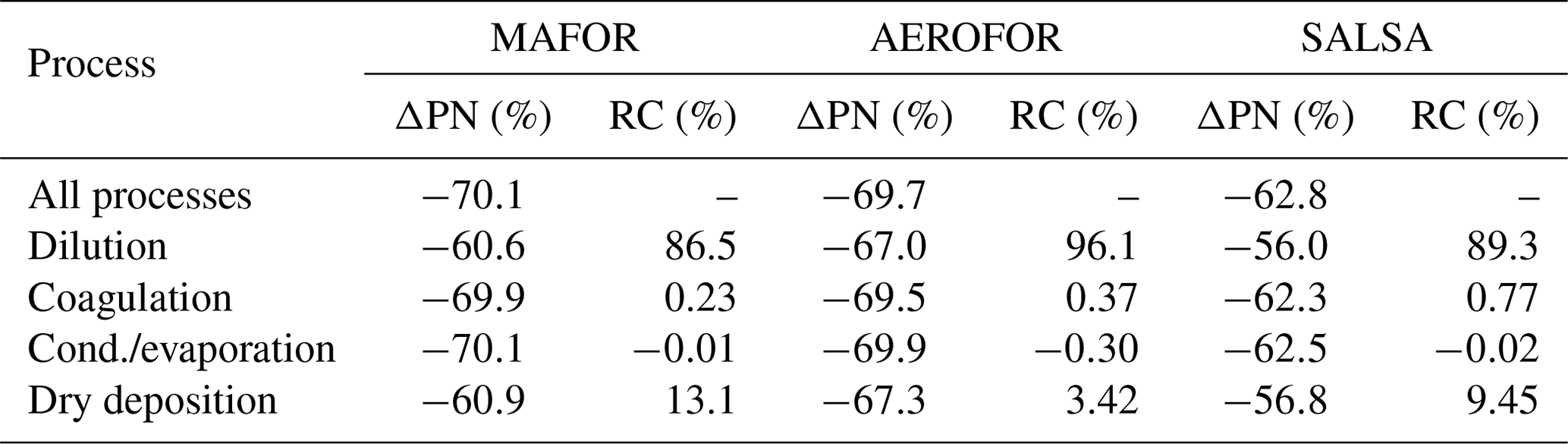
LNMOM-DC was employed to estimate the relevance of coagulation in the Urban Case by modelling the coagulation–dispersion system with an identical setup. The change in the total PN due to coagulation at 100 m of downwind distance was estimated to be less than 2 %. Due to the small impact of coagulation, LNMOM-DC could not be utilized further to calculate the change in the size distribution parameters due to coagulation.
Condensation and evaporation contributed almost negligibly to PN changes but effectively increased total PN (negative RC value; Table 8). Under inefficient dispersion conditions, an increase in total PN due to condensation has been noted previously by Karl et al. (2016) in a study of aerosol processes on the neighbourhood scale. While condensation of vapours is not expected to change the total number concentrations, it serves to increase the volume of particles (Seinfeld and Pandis, 2006) and can modify the shape of particle size distributions. The increase in total PN is related to the competition between condensation and dry deposition or coagulation: small particles that grow by condensation as the air parcel moves away from the emission source will be less affected by removal through deposition or coagulation.
The results on the importance of aerosol processes from the three models in this study agree with the general notion that dilution dominates over other processes and that dry deposition onto the road surface is the only competitive aerosol process that alters total PN concentrations and size distributions related to vehicular traffic emissions in a street canyon (Kumar et al., 2011).
One method of determining the relative importance of various processes is timescale analysis (Ketzel and Berkowicz, 2004). Timescale analysis for a street canyon in Cambridge, UK, showed that timescales were of the order of 40 s for dilution, 30–130 s for dry deposition on the road surface, 600–2600 s for the dry deposition on the street walls, about 105 s for coagulation, and about 104–105 s for condensation (Kumar et al., 2008). The timescale analysis by Nikolova et al. (2014) based on results from CFD modelling for an urban street canyon in Antwerp, Belgium, showed that the timescale for coagulation was about 3 times longer than for dilution, while the timescale for dry deposition was close to that of dilution under low-wind-speed conditions.
The importance of coagulation in street canyons is subject to ongoing controversy. The relevance of coagulation may depend on a variety of different factors, such as exhaust emissions, meteorological conditions, canyon geometry, and complexity of the area (Kumar et al., 2011). The timescales for self-coagulation and inter-modal coagulation of nucleation-mode particles are typically longer than the timescales for dilution (Kerminen et al., 2007; Pohjola et al., 2007). Kerminen et al. (1997) concluded that under conditions characterized by exceptionally slow mixing, simultaneous processing of ultrafine particles by dilution, self- and inter-modal coagulation, and condensation and evaporation can occur. Karl et al. (2016) found that coagulation was relevant for street environments in situations when large numbers of small particles (diameter <50 nm) from vehicle exhaust emissions co-occurred with a significant PN fraction of larger particles (diameter >100 nm). Kerminen et al. (1997) estimated the timescale for inter-modal coagulation of particles with Dp=10 nm to be 900–1200 s during rush hours, which is short enough to allow moderate removal of nucleation-mode particles by inter-modal coagulation.
4.1.3 Effect or influence of condensation and evaporation of organics
In the following, the relevance of condensation and evaporation of organic vapours in the Urban Case scenario is analysed with the MAFOR model. Condensation and evaporation are potentially important processes in the urban case simulation because condensable vapours are first emitted from the vehicles, then condense to primary emitted particles inside the street canyon, and eventually re-evaporate from the condensed phase as the air parcel moves away from the street. Condensation and evaporation do not change the total number concentrations but will alter the size distributions and particle volume. According to Kumar et al. (2011), the effect of condensation in street canyons is uncertain, especially regarding the sub-10 nm particles. Evaporation reduces the volume concentration of particles. Partial evaporation can also increase the rate of coagulation by increasing the diffusion coefficient of the remaining particles (Jacobson et al., 2005).
The uncertainties of condensation and evaporation in the models are partly attributable to the algorithm of the condensation process (e.g. mass accommodation coefficient in Eq. 4) and partly to the properties of the condensing or evaporating vapours (e.g. volatility of the chosen substances, vapour pressures of the liquid). In addition, the emission of semi-volatile organic vapours by vehicles is highly uncertain. Several sensitivity runs were done with MAFOR to evaluate the effect of uncertain parameters in the condensation of organic vapours. The evaluation of modelled size distributions was done by grouping particle sizes into six size categories (size classes S1–S6; see Karl et al., 2016).
Sensitivity runs with MAFOR were as follows.
-
C0(SVOC) ×100
-
Replace SVOCs by adipic acid (C0=0.95)
-
Accommodation coefficient for organics: 0.1
-
EFSVOC×20
-
EFSVOC×50
Table 9Effect of the chosen parameters for the condensing organic vapour(s) in the MAFOR model when simulating the Urban Case scenario (all processes included). The reference is the model run with all processes presented in Sect. 4.1.1. The size ranges of the six size classes are S1: 1–10 nm, S2: 10–25 nm, S3: 25–50 nm, S4: 50–75 nm, S5: 75–100 nm, and S6: >100 nm.
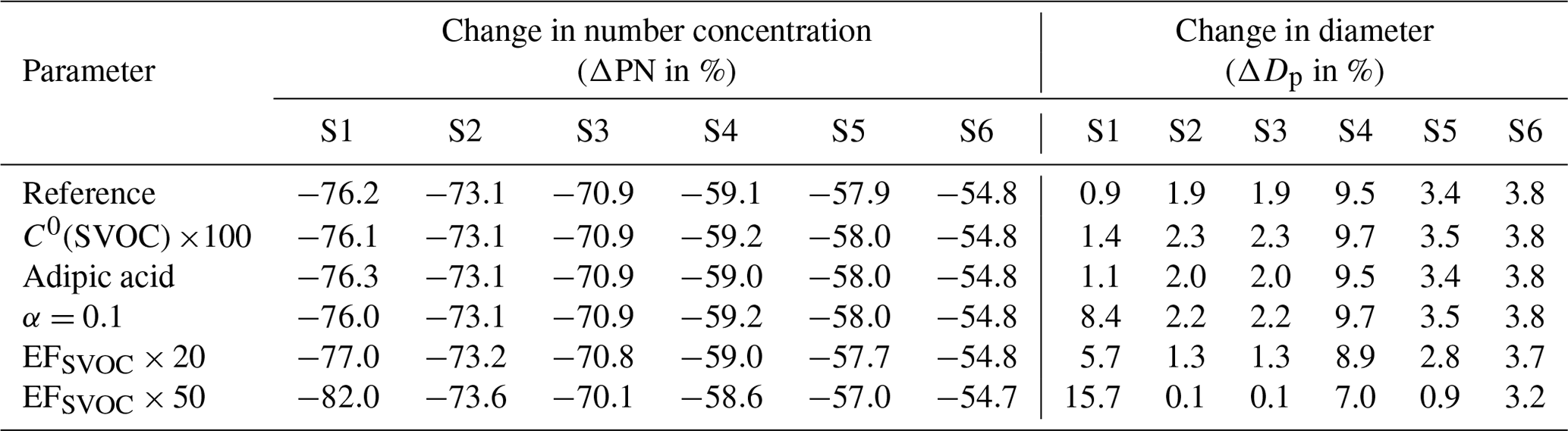
The model run with all processes presented in the previous sections is used as a reference. Results are shown in Table 9. The sensitivity tests reveal that uncertainties associated with the properties of the organic vapour(s) affect only the sizes of particles that are smaller than 10 nm, and these do not limit the ability to simulate most of the number size distributions and total PN concentrations. Even a 20-fold increase in SVOC emissions only affects the sub-10 nm particles. A 50-fold increase in SVOC emissions results in clear growth of <25 nm particles, mainly to sizes of 75–100 nm. The chemical composition of the traffic exhaust aerosol at points A and D computed with MAFOR indicates that condensation of organic vapours in the high emission case leads to uniform mass increases in the size range 20–200 nm compared to the reference (Fig. 14).

Figure 14Aerosol chemical composition obtained from the MAFOR model, given as mass concentration per size bin, in the Urban Case scenario: (a) reference simulation at point A; (b) simulation EFSVOC×50 at point A; (c) reference simulation at point D; and (d) simulation EFSVOC×50 at point D.
Modelled and measured mass size distribution of total particles at different distances from the edge of the road in the reference run and the sensitivity runs is presented in Appendix G and Fig. G1. The highest emission rate of SVOCs clearly leads to an overestimation of the measured mass concentration in the size range below 100 nm diameter. The simulations with MAFOR therefore allow estimating the magnitude of vehicle-emitted organic vapours to be on the order of 10−7 to 10−6 .
4.2 Discussion
4.2.1 Uncertainties in the Urban Case scenario
Computation of the aerosol evolution within the street canyon environment of the Urban Case scenario involves several assumptions and uncertain parameters. In the following the uncertainties of the processes and the design of the street canyon scenario are discussed.
Dry deposition is identified as the most important aerosol process in the Urban Case; at the same time, the size dependence of the dry deposition velocity is very uncertain. Measurements of dry deposition velocities for one particular surface type generally vary by 1 order of magnitude for a given particle size range of half of a logarithmic decade (Petroff et al., 2008). The HS2012 scheme used in the model is representative for dry deposition to rough environmental surfaces, which results in higher deposition velocities than for the other two aerosol dynamics models. The relative contribution on average of the three models was 9.7 %; together with an uncertainty of ±60 % (Karl et al., 2016), the RC of dry deposition could be as high as 15 %. The Zhang et al. (2001) parameterization used in SALSA predicts a size-dependent deposition velocity with a minimum at particle diameters of ∼1 µm, but measurements over vegetated surfaces suggest that the deposition velocity minimum occurs closer to ∼0.1 µm at the lower bound of the accumulation mode (Emerson et al., 2020). Dry deposition onto the road surface and/or building walls in a street canyon is mainly influenced by traffic movement and can reduce total PN concentrations by about 10 %–20 % (Gidhagen et al., 2004; Kurppa et al., 2019).
Brownian coagulation was identified as a minor aerosol process. While the timescales for coagulation of nucleation-mode particles is typically longer than the timescales for dilution, the effect of fractal geometry may enhance the coagulation rates. For small particles, fractal geometry enhances the coagulation kernel with increasing size of the colliding particle compared to spherical shape. A preliminary test of fractal geometry (rs=13.5 nm and Df=1.7) in a model run for the Urban Case (all processes included) resulted in PN reduction 0.2 % higher compared to compact particles. This suggests a higher importance of coagulation but does not change the conclusion that coagulation is a minor aerosol process in the Urban Case.
Evaporation might play a role in removing small particles and shrinking larger particles (Harrison et al., 2016), but the low temperature applied in the Urban Case scenario favoured condensation over evaporation. Uncertainties associated with the properties of the organic vapour(s) may affect the sizes of sub-10 nm particles. In particular, using a lower mass accommodation coefficient (α=0.1) for the organic vapour(s) may suppress condensation on small particles (Fig. G1), since more vapour molecules reflect from the particle surface back to air. However, molecular dynamics simulations and measurements indicate that the accommodation coefficient of atmospherically relevant organics is consistent with α=1 (nearly perfect accommodation), regardless of the molecular structural properties (Julin et al., 2014).
Traffic-originated particles in the diameter range of 1.3–3.0 nm, so-called nanocluster aerosol (NCA), have been measured in different traffic environments (Rönkkö et al., 2017). Hietikko et al. (2018) reported a clear connection between NCA concentrations and traffic volume in a street canyon. In the M2 street canyon, no significant number concentrations of particles with a diameter less than 4 nm have been observed. The measurement techniques of the instruments used, i.e. nano-SMPS and ELPI, are not suitable for detection of these small particles. The formation mechanism of NCA particles is not fully understood. It has been hypothesized that depending on the after-treatment systems of vehicles NCA represents non-volatile nano-sized particles formed in the combustion process in the cylinder or exhaust manifold or formed by an atmospheric nucleation mechanism during the dilution process of the exhaust (Järvinen et al., 2019; Alanen et al., 2015). The model is not able to simulate solid particles that form in the early stage of the engine exhaust. Nor did the sulfuric-acid-driven (atmospheric) nucleation produce these small particles (Sect. 3.3). Currently, the relative contribution of traffic-emitted NCA versus atmospheric nucleation to the formation of clusters and/or particles in this size range is not known and very likely depends on the driving conditions and environmental factors. Based on model calculations, condensational growth of NCA to larger sizes is more important than removal by coagulation on the street scale (Kangasniemi et al., 2019).
In the coupled dilution–aerosol process modelling of the present study, an average line source is assumed so that high particle emissions from certain vehicles (e.g. trucks or buses) are not considered. Gidhagen et al. (2004), using a CFD model for a street canyon, found a relatively high influence of coagulation on the removal of particles inside a street canyon. For a wind speed of 2 m s−1, the effect of coagulation on total PN was 15 % at the leeward side and 21 % at the windward side. The reason for the higher influence of coagulation might be the more realistic simulation of dispersion in the street canyon, resulting in a longer residence time of particles inside the street canyon. The CFD simulation considered the plumes of all vehicles inside the street canyon (diluted with clean air), which enhances the effect of removal by coagulation because coagulation is more efficient close to the particle source. The average dilution timescale in the Urban Case (from road edge to point D) was 31 s, which is close to the dilution timescale of a real street canyon at a wind speed of 3 m s−1 (Nikolova et al., 2014). For low wind speeds and low traffic intensity the dilution timescale in a street canyon with a unit aspect ratio is typically 120 s (Ketzel and Berkowicz, 2004). With a longer residence time in the street canyon, processing of ultrafine particles by coagulation and condensational growth would be more relevant.
Based on the national calculation system for traffic exhaust emissions and energy consumption in Finland (LIPASTO, 2021), the average exhaust emission of PM2.5 by vehicles in 2010 was on average 1.5–2.9 times higher than that in 2017 (the reference year of EFPN used in the present study). The decreasing trend is qualitatively in agreement with the corresponding data in Fig. 6 in Kukkonen et al. (2018); however, that figure only addresses developments until 2014. Ultrafine particles originate from exhaust emissions, so those have probably diminished in time, mainly due to the implementation of diesel particulate filters. How much exactly is not known, as this depends on the development of engine technology, fuels, and other factors. Model simulations of the Urban Case show that the EFPN from 2017 is in accordance with the total PN concentrations measured in the street canyon.
4.2.2 Discussion of model performance
Statistical performance indicators in the comparison of model data against observation data in the Urban Case scenario provide an unambiguous criterion for evaluating the performance of MAFOR in comparison to that of other models. The results on the statistical performance of the model with respect to total PN, number size distribution, PM1, and BC are summarized here.
-
The model reproduced the reduction of total PN concentrations with increasing distance from the street in excellent agreement with the experimental data.
-
The model performs well for the number size distributions at street level and different distances from the street despite the coarser resolution of the particle emission size spectrum from vehicles.
-
The model performed weaker for PM1, but the mean error of the prediction is still acceptable given the high relative uncertainties of the measurements. The low predictability of the observed PM1 variation is partly attributed to the long averaging interval of the measurements (ca. 5–10 min) compared to the instantaneous model simulation.
-
The model performs fairly well for BC, but varying traffic conditions may have affected the measurements, making the M–O comparison for BC less reliable.
Overall, the simulation of the Urban Case demonstrates the good performance of MAFOR v.2 in predicting particle number, size distribution, and chemical composition of traffic exhaust aerosol. A major advantage of the model is the consistent treatment of particle number concentrations and mass concentrations of each aerosol component through the simultaneous solution of aerosol dynamics processes in terms of number and mass. This procedure allows the changes in the average density of particles to affect the predicted number and mass size distributions. An added value of the model is that it can be used to determine the (order or magnitude) emission rate of SVOCs by comparison between the modelled and the observed size distribution of total mass.
In addition to the statistical model performance of the aerosol process models presented in Sect. 4.1.1, we define a set of additional criteria for the overall evaluation. Clearly, this is not a strength-and-weakness analysis because model user feedback cannot be provided at the current stage. The additional indicators are intended to characterize the capabilities of the models in an objective way to be comparable between the models. The selected additional criteria are
-
computing time,
-
comprehensiveness of model outputs, and
-
representation of aerosol chemical composition.
Computing time is an important criterion for comparing the computational efficiency of models and algorithms. Computer models that have an excessive demand of time are less attractive for the model user and are usually not suitable for integration in 3-D models. The computational time on a single CPU for the base simulation of the Urban Case scenario (all processes included) for a plume travel distance of 120 m was 1.5 min for MAFOR (Linux mini PC, 7.6 GB RAM), 1.2 min for SALSA (Linux desktop PC, 32 GB RAM), and 5.2 min for AEROFOR (desktop PC, Windows XP, 2.96 GB RAM, year 2002). Since the different aerosol dynamics models were run on different computers it is not possible to give an accurate ranking of the time required by each model. Nevertheless, roughly comparing the computational times of the models indicates that MAFOR runs with similar speed as SALSA.
Particle number size distribution is the basic output of all models. Additionally, model output of MAFOR comprises size distributions of total mass and the chemical composition (mass fractions). SALSA outputs volume size distributions of particle components, which at known density can be translated to mass concentration. An added value of MAFOR is the capability to resolve the chemical composition of each size section in terms of mass, which allows the size-resolved quantification of the condensed mass of volatile species within the full diameter range.
Regarding the speciation of the aerosol chemical composition in the models, MAFOR has a similar degree of detail and capabilities as SALSA, with the addition that two organic vapours (optionally three) of different volatility were used to represent condensation and evaporation of SVOCs. AEROFOR used two condensable vapours (H2SO4 and SVOCs) to describe the condensation and evaporation to an internally mixed aerosol, with all particles containing both compounds. In MAFOR and SALSA, the composition of the background aerosol (sulfate, BC, mineral dust, sea salt, etc.) can be defined separately from the composition of exhaust emissions.
4.2.3 Consistent treatment of mass- and number-based concentrations of PM
The consistent treatment of mass- and number-based concentrations of particulate matter in the model has several aspects:
-
initialization of the aerosol size distribution,
-
insertion of particles from aerosol source emissions,
-
mathematical solution of the aerosol dynamics processes, and
-
comparability to both the observed PM mass and number concentrations.
In the MAFOR model, the aerosol is initialized based on the modal mass composition, which is then distributed over the size bins of the model (Eq. 21) and converted to number based on the material density of the different aerosol components, assuming spherical particles.
This procedure ensures that the initial aerosol is consistent in terms of mass and number. The model simultaneously solves the number concentrations and mass concentrations for each size section as they change with time due to different aerosol dynamics processes in a given scenario. This method has two advantages: (1) it takes into account the concurrent change in average particle density during the evolution of an aerosol size distribution in the prediction of number and mass concentrations, and (2) it represents the growth of particles in terms of both the number and the mass. Finally, the output of modelled particle number size distribution and mass concentration size distribution can be directly compared to observed number and mass concentration size distributions, respectively.
Some of the above-mentioned aspects have uncertainties and limitations, which results in a certain deviation from the full consistency of number and mass.
In the real-world scenario in a street canyon environment (Urban Case), particle emissions are reported on the basis of numbers. However, the emissions in the MAFOR model are mass-based, and these are subsequently converted to number-based using assumptions on their densities. The total PN emission factor is dependent on the setups of the measurements (Kukkonen et al., 2016). First, the emissions may include either only solid particles or solid and volatile PN; second, the PN emission factor has a variable lower particle size cut-off, depending on the employed instrumental method.
In the case of the street canyon simulation, the PN emission factor was adopted from Kurppa et al. (2020) and emissions were distributed over the particle size distribution. This was done so that the modelled size distribution after a distance of 5.5 m from the start matched the measurement of the particle size distribution at street level. A limitation of this modelling was that the particle emissions were attributed to a modal distribution in MAFOR. The MAFOR model represented the variation of particle emissions between different size bins less well than the two other models, SALSA and AEROFOR, which used a bin-wise representation, in particular for the particles with sizes below 20 nm diameter.
When comparing the modelled total particle mass concentration distribution to observations from ELPI in the Urban Case (see Fig. 12), we have assumed that all particles were spheres and had the same density of 1000 kg m−3. The ELPI charging efficiency depends on particle mobility diameter, whereas the ELPI measures the aerodynamic diameter of particles. This dilemma is usually circumvented by assuming that the particles are unit density spheres, for which mobility diameter equals aerodynamic diameter. For soot particles that form as agglomerates of approximately spherical primary particles with 10–30 nm diameter, the effective density decreases with particle growth. This in turn narrows their aerodynamic size distribution relative to their mobility distribution. The uncertainty due to changes in effective density of soot particles is estimated to cause a systematic error for the determination of PM with ELPI of about 20 % (Maricq et al., 2006). Salo et al. (2019) compared ELPI+ to PM10 cascade impactors in combustion emission measurements. ELPI+ mass concentrations were larger for most combustion cases, probably because the effective density of the particles was not the assumed unit density and because volatile particles were measured by ELPI+, but not with the cascade impactors.
DeCarlo et al. (2004) mention two issues that affect the conversion of particulate matter mass to numbers: ultrafine particles with irregular shape and the internal void volumes of diesel soot agglomerates. Therefore, the evaluation of modelled total mass concentration in comparison against the measurements relies on the assumption of spherical particles without internal voids.
4.2.4 Evaluation of the model improvements
The Urban Case scenario was selected for the evaluation of the model because it considers the scale between the release of exhaust and the roadside, for which the aerosol dynamics processes are typically not resolved in city-scale dispersion models. Semi-volatile organic vapours can grow nucleation-mode particles with a non-volatile core that formed in the vehicle exhaust before the dilution process, without any significant chemical transformation in the atmosphere (Rönkkö et al., 2013). The improved treatment of semi-volatile organic compounds in MAFOR v2.0 with respect to their volatility distribution and their role in the growth of small particles was evaluated in Sect. 4.1.
However, it was not possible to evaluate SOA formation through VOC photo-oxidation because the gas-phase concentrations of VOCs in the street canyon environment have not been measured. In follow-up work, it is planned to evaluate the performance of MAFOR v2.0 in simulations of secondary aerosol formation in aged vehicle exhaust in a smog chamber experiment or in an oxidation flow reactor (OFR). The model evaluation will be designed to consider the production of SOA precursors from the oxidation of VOCs using the mass-based formulation of the embedded 2-D VBS framework for organic aerosol-phase partitioning.
The simulation of SOA formation with coupled photochemistry and aerosol dynamics has previously been evaluated in a smog chamber experiment for the OH-initiated oxidation of 2-aminoethanol (Karl et al., 2012b). In the applied version of the MAFOR model, the coupling was with the gas-phase chemistry scheme of MECCA v3.0. The main advantage of using the new version 4.0 of MECCA in MAFOR v2.0 is the much more detailed VOC chemistry of the Mainz Organic Mechanism (MOM). In a study of the oxidation processes in the Mediterranean atmosphere, simulated atmospheric OH concentrations with the CAABA/MECCA box model using MOM chemistry were in good agreement with in situ OH observations (Mallik et al., 2018).
The performance of the improved coagulation kernel in MAFOR v2.0 was analysed in the simulation of a chamber experiment in the presence of continuous emission of nanoparticles (Case 2). For details, we refer to Sect. S3. When assuming compact spherical particles, the simulation of the evolution of the particle size distribution due to Brownian coagulation was in good agreement with the modelled particle size spectra and total particle number concentrations for the same case published in Anand et al. (2012). When fractal particles are considered in the model (Df=1.75), the resulting particle size distribution is similar to the same case of Anand et al. (2012); however, growth of the fractal particles into a secondary mode is less efficient (Fig. S3). Differences in the coagulation efficiency probably lie in the details of the implementation of the fractal geometry in the coagulation kernel, although the same particle morphology was used in the present evaluation. The coagulation solution with respect to particle mass conservation is sufficiently accurate, with an error of less than 0.5 %.
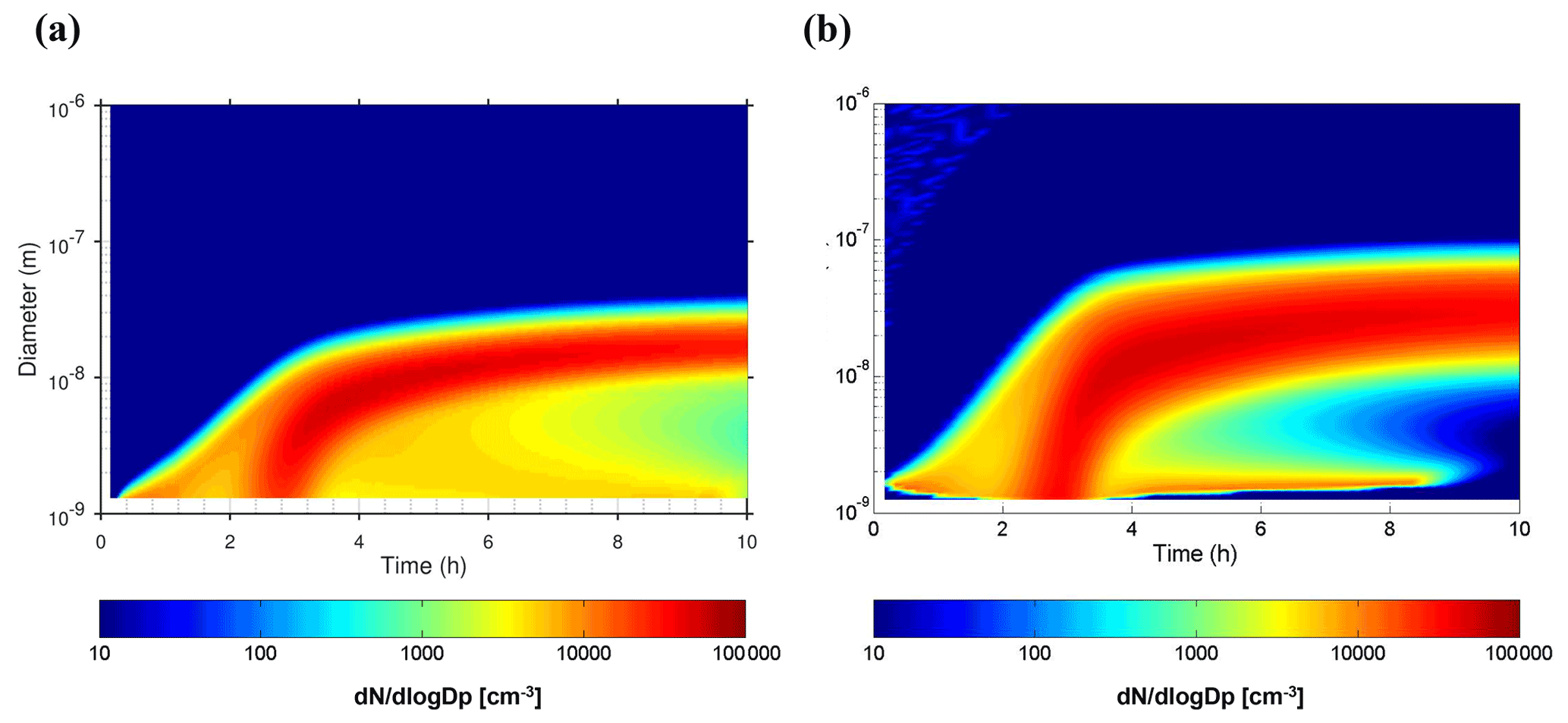
Figure 15Evolution of the modelled particle number size distribution in a 10 h simulation to compare the performance of the nucleation code M2018 in (a) MAFOR v2.0 to that in (b) AEROFOR. New particles were inserted at 1.0 and 1.5 nm diameter in MAFOR and AEROFOR, respectively. The first particle formation after 15 min is due to ion-induced nucleation, and the main particle burst after 2 h is due to neutral nucleation. Final mean Dp was 18 and 22 nm, respectively, in MAFOR and AEROFOR simulations. Details on the configuration of the numerical experiment are given in Appendix H.
The performance of the new binary parameterization of Määttänen et al. (2018a, b; M2018) in MAFOR v2.0 was compared to the AEROFOR model, as described in Appendix H. Simulation of particle formation was evaluated in a numerical experiment with zero background particles, mimicking conditions over the high Arctic in summer characterized by a very low number of pre-existing particles and low temperatures (Mauritsen et al., 2011; Karl et al., 2013). A particle burst occurred in simulations with both models 2 h after the beginning due to neutral nucleation. The maximum nucleation rate, total particle (Dp>3 nm) number concentration, and H2SO4 concentration calculated by MAFOR agreed well with results from AEROFOR (Fig. G2). Growth of the nucleated particles in MAFOR was weaker and resulted in a size band of new particles that was narrower than in the simulation with AEROFOR (Fig. 15). The weaker particle growth might be attributed to differences in the treatment of sulfuric acid condensation and particle deposition.
The coupled PNG–MOSAIC system that enables dynamic dissolution and evaporation of semi-volatile inorganic gases (Sect. 2.4) was tested in numerical scenario calculations with different initial concentrations of NH3 and HNO3 at RH = 90 % (Case 3), as described in Supplement Sect. S4. The initial conditions for Case 3 were adopted from the tests of the PNG–EQUISOLV II scheme presented in Jacobson (2005a). In simulations of Case 3, H2SO4 was condensed, HCl and HNO3 were dissolved and/or dissociated, and NH3 was equilibrated with dissolved and dissociated species. Uptake of water occurred at each model time step based on equilibrium thermodynamics. Under conditions of high concentrations of both NH3 and HNO3, an equilibrium was reached within about 6 h, and the time-dependent summed concentrations of inorganic aerosol species matched the equilibrium levels from EQUISOLV II fairly well (Fig. S2 in the Supplement). Under low nitrate conditions, the performance of the PNG–MOSAIC scheme is very accurate. Under low ammonia conditions, the simulated time series of summed concentrations of inorganic aerosol species from MAFOR are smooth, showing no sign of oscillation, and the model achieves similar accuracy as PNG–EQUISOLV II.
4.3 Planned developments for MAFOR
The future development of MAFOR beyond version 2.0 in view of application in urban settings is briefly outlined in the following. Specifically, the further improvement for application of the model in plume dispersion scenarios and the integration in 3-D atmospheric models on the urban scale will be the focus of the planned development for the next versions of MAFOR.
4.3.1 Plume dispersion simulation
The processes relevant for simulating urban cases and the emissions from mobile transport sources are in the focus of the upcoming development. The following topics will be addressed in the continued development of the model.
-
Currently, the size spectra of particle emissions can only be represented in four modes. Improving the size resolution of particle emissions (bin-wise) in the model has high priority.
-
Traffic-originated NCA particles may be formed via a delayed primary emission route by rapid nucleation of low-volatility vapours (e.g. primary emitted H2SO4) during exhaust cooling after release from the tailpipe (Olin et al., 2020), or they are directly emitted as solid particles (Alanen et al., 2015). While the emission of nano-sized solid particles is already implemented (Karl et al., 2013), it is envisaged to implement the delayed primary route in the model to test this hypothesis.
-
Ammonia emissions from road traffic represent an emerging issue (Farren et al., 2020); NH3 is released from catalyst-equipped gasoline vehicles as well as light-duty and heavy-duty diesel vehicles that rely on selective catalytic reduction (SCR). Vehicle emissions of NH3 may affect new particle formation via the ternary route and secondary aerosol formation in urban areas. It is planned to activate the PNG–MOSAIC module in plume dispersion runs in order to simulate SIA formation in vehicle exhaust plumes.
-
Soot particles acquire a large mass fraction of sulfuric acid during atmospheric ageing. Condensation of H2SO4 to soot particles was shown to occur at a similar rate for a given mobility size, regardless of their morphology (Zhang et al., 2008). Coating of fractal soot agglomerates with H2SO4 and water is accompanied by restructuring to a more compact form. The change in fractal dimension and effective density during soot ageing will be implemented in the model.
-
Additional dilution schemes for ship exhaust for ocean-cruising vessels may be implemented. Chosson et al. (2008) proposed a dilution parameterization for use in CTMs based on sophisticated methods to represent dilution in boundary layers by taking into account the initial buoyancy flux of the ship exhaust. For close-to-stack dispersion, the current method in Karl et al. (2020) is considered to be more suitable (Sect. 2.7).
-
Particles from ship exhaust can act as CCN. Aerosol activation will be implemented in the model based on the scheme of Abdul-Razzak and Ghan (2002) with a sectional representation. Instead of using a single-parameter representation for hygroscopicity growth (Petters and Kreidenweis, 2007), the dynamically calculated concentrations in the liquid droplet will be used.
With the proposed implementations, it is ensured that the model will remain state-of-the-art and could even become a benchmark model for aerosol dynamics process simulations.
4.3.2 Integration in 3-D atmospheric models
Implementation of the presented aerosol dynamics module into 3-D atmospheric dispersion models is facilitated by the operator splitting of processes and by the efficient integration of particle number and mass concentrations. The fixed sectional method is the most practical way to consider continuous nucleation of new particles together with the atmospheric transport and emission of particles. Coagulation is the process with the highest computational demand due to the representation of collisions of a particle from one size section with particles from all other sections. It will be considered in the future to implement an adaptive time stepping scheme for solving the coagulation process.
With regard to implementation of the aerosol dynamics code into large-scale atmospheric models it is of special interest to assess how much one can lower the accuracy of the size distribution description without compromising on the accuracy of the model results. The evaluation of the sectional size representation in Case 1 (Sect. S2 in the Supplement) revealed that the use of 16 size sections causes a numerical error of ∼10 %, and the use of 32 size sections causes an error of only ∼3 % in the final total PN concentrations under those conditions. The error of both representations is considered still acceptable when compared to measurement errors of observed total PN concentrations. Further, the computational demand increases only slightly when using a larger number of size sections. Overall, the size representation using 32 size sections is adequate for the simulation of long periods, as the accuracy in terms of size distribution changes and total number concentration is sufficiently high, while the computational demand is only 2 % higher compared to the lowest tested resolution of 16 size sections.
Aerosol representations in large-scale models are often limited to fewer than 20 size classes, as the particles in each size section have to be included in the advection routine and a higher number of advected species increases the computing time. Therefore, methods need to be developed for the mapping of the size representation used in the aerosol dynamics code and the advected particle species. The effect of changing the number of size classes in 3-D model needs to be tested thoroughly.
Studies have demonstrated the relevance of episodes of new particle formation in cities situated in high insolation regions such as southern Europe. Both photo-induced nucleation and traffic emissions play a critical role in determining UFP concentrations in cities (Rivas et al., 2020). In addition, there is the highly dynamic sequence of chemical and physical processes such as condensation, deposition, and coagulation that modulates the number size distributions, making modelling of UFP concentrations on the city scale a complex task.
It is planned to integrate the aerosol dynamics code into the open-source city-scale model EPISODE-CityChem (Karl et al., 2019). The first requirement is the implementation of a size-resolved particle number emission inventory that compiles PN emission factors and size distributions for different sectors (e.g. Paasonen et al., 2016). The basic assumption of these PN emission inventories is that all primary particles are non-volatile and composed of the same material, although one could assume a certain fraction of particles (in each size section) to be either BC, OC, or a different material. According to this definition, volatile particles would always be secondary particles, i.e. forming in photo-induced nucleation or by condensation of gases already existing in the atmosphere, ignoring the fact that volatile particles may also form rapidly very close to the source of emissions, on the sub-grid scale of the 3-D model (grid resolution typically 100–1000 m). Nevertheless, the division into primary non-volatile particles and secondary volatile particles serves as a good starting point for the implementation of aerosol dynamics in the city-scale model.
There are certain specifications of the MAFOR box model that need to be retained in the large-scale model: (1) the structure of the four aerosol modes (nucleation, Aitken, Accumulation, coarse) with each mode divided into the same number of size sections and (2) the consistency between number and mass calculations. Condensation and evaporation of a chemical species in MAFOR adhere to the mass balance between gas phase and particle phase. Therefore, the mass concentration of the condensing species in each size section has to be considered an additional model species. If, for instance, 16 tracers for PN (16 size classes) are used, then the condensation of a single gas species will require the addition of 16 tracers for mass concentration. For computational reasons, one should aim to restrict the variety of chemical aerosol components as much as possible, for example by lumping all components of primary emitted particles (BC, primary OC, sea salt, etc.) into one single non-volatile model species, consistent with the PN emission approach outlined above.
The MAFOR box model inherently includes coupling to a detailed gas-phase chemistry. However, the aerosol dynamics solver can be applied as a separate module in 3-D atmospheric models. The treatment of secondary organic aerosol by a hybrid approach in MAFOR (Sect. 2.5) is already in line with possible implementation in 3-D models. For the implementation in an atmospheric model it is important to connect the vapours to their origin and source region, e.g. biogenic versus anthropogenic, for later research applications. The chemistry solver of the 3-D model needs to be modified to account for chemical reactions that lead to the production of gaseous precursors, or a subset of these, involved in SOA formation (Fig. 7).
The open-source aerosol dynamics model MAFOR v2.0, as a new community model, was described and evaluated against measured data, and the predictions were intercompared with those of two other aerosol process models.
The main new features of MAFOR v2.0 compared to the original model version (v.1) are the following. (1) The model has been coupled with the chemistry module MECCA, comprising detailed up-to-date photolysis rates of VOC chemistry. This allows the partitioning of chemical species and the subsequent aqueous-phase reactions in the liquid phase of coarse-mode particles. (2) The model includes a revised Brownian coagulation kernel that takes into account the fractal geometry of soot particles, van der Waals forces, and viscous interactions. (3) The model contains a multitude of state-of-the-art nucleation parameterizations that can be selected by the model user. (4) The model has been coupled with PNG–MOSAIC, enabling size-resolved partitioning of semi-volatile inorganics at a relatively long time interval. (5) The model includes a hybrid method for the formation of SOA within the framework of condensation and evaporation. These features make the model well suited for studying changes in the emitted particle size distributions by dry deposition, coagulation, and condensation and evaporation of organic vapours in urban environments as well as for the simulation of new particle formation over multiple days.
The performance of MAFOR v2.0 was evaluated against field-scale measurements of plume dispersion in a street environment located in the centre of Helsinki, published by Pirjola et al. (2012). The experimental data were obtained with a mobile laboratory van at different locations in the street environment. The data included particle number measurements in the size range of 3–414 nm, black carbon, and fine particulate mass PM1. The model was also intercompared with the results from two other aerosol dynamic models (AEROFOR and SALSA). MAFOR reproduced the reduction of total number concentrations with increasing distance from the street in good agreement (IOA = 0.85) with observations. MAFOR performed well in predicting the number size distributions at street level and at different distances from the street (average IOA = 0.78), and it was able to reproduce the development of the size distributions with increasing distance better than AEROFOR and SALSA. A limitation of MAFOR is that it represents the particle emission size spectrum as a multi-modal distribution, which may result in an underestimation of the number of small particles, while the total number of emitted particles is not affected. MAFOR predicted the variation of fine particulate matter PM1 (IOA = 0.25) in the street environment in better agreement with experimental data than SALSA. The difficulty in predicting the variation of observed PM1 is related to the long averaging interval of the mass measurements compared to the model simulations that reflect instantaneous concentrations.
Dry deposition was found to be the only aerosol process that can compete with dilution, in agreement with several previous aerosol process studies in street canyons. Brownian coagulation played a minor role, and this was also confirmed by a simulation with the dispersion–coagulation code LNMOM-DC. Longer residence time in the street canyon and higher-than-average emissions from certain vehicles may increase the relevance of self- and inter-modal coagulation of nucleation-mode particles. For future aerosol process modelling studies in urban environments it is recommended to (1) select an appropriate deposition scheme based on the environmental conditions, (2) parameterize the dilution rate based on turbulence-resolving CFD simulations, and (3) constrain the particle emission size spectrum by independent measurements in the same environment.
The early phase of the vehicle exhaust plume was not resolved in this study. The vehicle wake is the first spatial scale from which the emitted UFPs will disperse into the ambient environment (e.g. Kumar et al., 2011). The parcel of exhaust emission at the tailpipe contains pre-existing particles from fuel combustion, unburnt droplets from lubricant oil, and various precursor gases for condensation. This parcel may already contain traffic-originated particles in the diameter range of 1.3–3.0 nm, so-called nanocluster aerosol (NCA) particles that were previously not detected by the instruments due their small size. Their origin might be either the direct emission of non-volatile particles that formed in the engine or the rapid nucleation of low-volatility vapours during exhaust cooling after the tailpipe. The delayed primary emission route to explain the formation of NCA during exhaust cooling should be implemented in MAFOR in the future. The subsequent growth of NCA by organic vapours also needs to be investigated; MAFOR could be an ideal research tool for this, as the model allows constraining the emission rate of condensable organic vapours based on the measured mass size distribution.
For the consideration of the aerosol processes in urban-scale 3-D models, a division into primary non-volatile particles and secondary volatile particles is proposed here as a starting point for the implementation of the aerosol dynamics code. The treatment of primary particles as non-volatile is consistent with current size-resolved PN emission inventories. The volatile particles form by nucleation, and both particle types grow by condensation of semi-volatile or low-volatility vapours. The division enables the mass-conserving approach to condensation and evaporation of vapours, and it allows minimizing the total number of aerosol chemical species in the 3-D model.
The continued development of the open-source code by the community is advised and steered by a consortium of aerosol scientists. Several aspects of the numerical solutions (efficient integration of number and mass concentrations, operator splitting of processes, use of the fixed sectional method, and low numerical diffusion) make the aerosol dynamics code a promising candidate for implementation into large-scale atmospheric models. Ultimately, it is intended to establish MAFOR v2.0 as a state-of-the-art benchmark model for evaluating aerosol processes in dispersion studies from local to regional and global scales. We encourage and support the integration of this aerosol dynamics code into urban-, regional-, and global-scale atmospheric chemistry-transport models, possibly also into Earth system models.
A list of the acronyms and abbreviations used in this work is given in Table A1. The nomenclature used in this work is summarized in Table A2.
A1 List of the acronyms and abbreviations used in this work
A2 Nomenclature used in this work
The Analytical Predictor of Condensation (APC; Jacobson, 2005b) obtains a non-iterative solution for the change in the gas-phase concentration of the condensable compound with time using the mass balance equation of the final aerosol- and gas-phase concentrations.
An equation that describes the condensational growth of a component q onto particles of size i is Eq. (8) in Sect. 2.3.2 (Jacobson, 1997b).
The mass transfer rate between the gas phase and all particles of size i can be approximated as , where Ni is the number concentration of particles of size i, ri is the radius of a single particle, Dq is the diffusion coefficient, and βq,i is the transitional correction factor.
For the dissolution process, the saturation vapour concentration is a function of particle composition, and the corresponding equation is (Jacobson, 1997b)
where is the equilibrium saturation ratio and is the dimensionless effective Henry's law coefficient for the respective size bin.
Mass is conserved between the gas phase and all size bins of the particle phase by respectively writing the gas conservation equations for Eqs. (B1) and (B2) as
Equations (B1) and (B3) together represent NB+1 ordinary differential equations for condensation and evaporation that are solved in the APC scheme. The APC solution follows from integration of Eq. (B1) to obtain the final concentration of compound q in size bin i. The resulting implicit expression for the mass concentration after a time step of condensational growth is
where the subscripts t and t−Δt indicate the current time and one time step backward, and Δt is the length of the (growth) time step. The final gas-phase concentration of the component is currently unknown.
Based on the mass balance equation, the total concentration Ctot,q of the compound in gas and particles is constrained by
Substituting Eq. (B5) in Eq. (B6) and solving for gives the final gas-phase concentration in the condensation process at the end of time step Δt:
where is the gas-phase concentration of compound q calculated at the end of the chemistry time step.
The concentration calculated from Eq. (B7) for condensation and evaporation cannot fall below zero but can increase above the total mass of the compound. Therefore, the gas-phase concentration is limited by , Ctot,q). This value serves as an estimate and is substituted into Eq. (B5).
It is problematic that Eq. (B5) can result in a negative aerosol mass concentration or in a concentration that exceeds the maximum (i.e. the total compound concentration). Therefore, two limits have to be placed subsequently after the computation of Eq. (B5). The first limit is = , 0) and the second limit is (Jacobson, 2005b)
where the values of on the right side of the equation are determined after the first limit has been applied for all size bins.
A solution for the growth by the dissolution process is given in Jacobson (2005a). Equations (B2) and (B4) together represent NB+1 ordinary differential equations for growth by dissolution. The solution to the equations of dissolutional growth is obtained by integration of Eq. (B4) to obtain the final mass concentration of component q in size bin i. The resulting expression is Eq. (16) in Sect. 2.4. The final gas-phase concentration in Eq. (16) is currently unknown.
Substituting Eq. (16) into the mass balance Eq. (B6) and solving for gives the final gas-phase concentration for dissolution at the end of time step Δt (Jacobson, 2005a):
The Analytical Predictor of Condensation, with the mass balance restrictions above, and the solution for the growth by dissolution are unconditionally stable, since all final concentrations for the gas and particle are bounded between 0 and Ctot, regardless of the time step.
In the model size distribution, particles from the first size section collide with particles from all other size sections. Particles from the second size section collide with particles from the third to largest size section, and so on. The number concentration of particles in section i, Ni, increases if the colliding particles result in a particle of the same size as particles in section i. It decreases if particles in section i coagulate with particles of other size sections or of the same section. When particles of volume υk and υj collide, the resulting particle has an intermediate volume . If the intermediate volume falls between the two size sections i and i+1, then the new particle is split between the two sections and constrained by volume conservation. Thus, a size-splitting operator, the volume fraction for the partitioning to each model section i, is defined as in Jacobson (2005b).
An advantage of this method is that the volume fractions obtained in Eq. (C1) are independent of the representation of the size distribution.
The free-molecular collision rate correction factor Wk of the coagulation rate due to van der Waals forces is given by
In the free-molecular limit, there is no viscous interaction between particles.
The van der Waals interaction potential E(r) is given by
where AH is the Hamaker constant, which is specific for the van der Waals properties of each substance. Here, the Hamaker constant of water, , is used for all particle types. The derivatives of the van der Waals interaction potential in Eq. (D1), and , are obtained using the MATLAB™ symbolic package.
The correction factor Wc in the continuum regime is
Viscous force correction of the diffusion coefficient in the continuum regime is
In Eq. (D4), is a relative diffusion coefficient between particles i and j, and = is the sum of the individual diffusion coefficients of the two particles.
The integral in the correction factors Wk and Wc is approximated by numerical integration using the Gauss–Legendre quadrature formula after transforming the variable r using the relation (with the dimensionless coordinate x) so that the limits of the integral become 0, and and can be evaluated as a function of x (where a=ri, b=rj; and b≥a).
The first dilution stage of the diluted exhaust plume, between the upwind curbside and the downwind curbside of the street, was described with the jet plume dispersion model of Vignati et al. (1999). In this model, dispersion of the plume is calculated taking into account the atmospheric turbulence, the traffic-generated turbulence, and the entrainment of fresh air due to the jet effect of the exhaust gas. The expression for the evolution of the plume cross section during the first dilution stage is given by
where S is the cross-sectional area of the air parcel or exhaust plume (in m2), S0 is the cross section of the initial air parcel (here: 0.8 m), σw(0) is the initial entrainment velocity (in m s−1), and u0 is the initial exhaust gas velocity (here: 0.23 m s−1).
The entrainment velocity is given by
where ustreet is the street-level wind speed, σwt is the traffic-generated turbulence, and ujet is the plume jet velocity. The proportionality constant α is set to 0.1, which is typical for mechanically induced turbulence (Berkowicz et al., 1997). The traffic-generated turbulence is estimated using the traffic count, street width, horizontal area of a vehicle, and typical vehicle speed.
The evolution of the plume height, Hp, during the first stage is derived from Eq. (E1), assuming a circular plume cross section:
The dilution ratio DR in the vehicle exhaust plumes increases approximately linearly with time during the first seconds of the dilution. The dilution ratio is given by
The change in the dilution ratio with time, , is obtained from the derivation of ,
The particle dilution rate as a function of time for the first dilution stage is
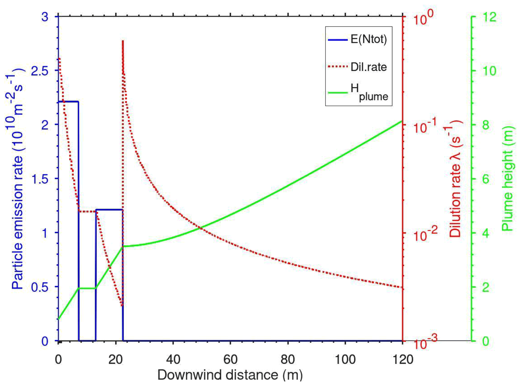
Figure E1Plot of emission rate of exhaust particles in 1010 (blue line), dilution rate, λdil, (red dotted line), and air parcel height (green line) as a function of time after simulation start in the Urban Case scenario. The plume height and the dilution rate are constant while the air parcel passes over the tram tracks in the middle of the street.
For the second dilution stage, between the downwind curbside and ambient environment, the dispersion situation was analysed with the simplified street canyon model SSCM, a component of EPISODE-CityChem (Karl et al., 2019) using realistic street canyon geometry, line source emissions of total particles in both directions of the street, and the meteorological conditions of the Urban Case. Modelled total PN concentrations were obtained at certain receptor points located perpendicular to the street in the downwind direction, beginning at the curbside, at distances of 10 m. A numerical power function was fit to the modelled PN concentration data. The resulting fit equation for total particle number concentration was found to be Ntot (cm−3) d−0.306, with downwind distance d from the curbside in metres (m). The dilution parameter is close to the reported value of 0.34 in Pirjola et al. (2012) that was derived from PN measurements. The obtained parameter b=0.306 is used in Eq. (25) to calculate the change in particle number concentration with time due to dilution in aerosol dynamics models.
The height of the air parcel containing the vehicle exhaust, as a function of time during the second dilution stage, is given by
where Hp,0 is the height of the plume at the end of the first dilution stage, while a′ and b′ are dispersion parameters and depend on the atmospheric stability. For stable conditions prevailing in the Urban Case scenario, and (Petersen, 1980) were chosen. The evolution of air parcel height, dilution rate, and particle emission rates during the Urban Case scenario simulation is shown in Fig. E1.

Figure E2Modelled particle number size distribution with MAFOR using different dry deposition parameterizations at point D (after 78.5 s of plume transport time). HU2012 is the reference dry deposition configuration used in MAFOR, SPF1985 is the dry deposition scheme in AEROFOR, and ZH2001 is the dry deposition scheme in SALSA. Measured size distributions from SMPS are shown as red circles.
To assess the differences in model results due to the application of different dry deposition schemes (Table 5), model runs including all aerosol dynamics processes and dilution were performed with the MAFOR model for the Urban Case scenario using the dry deposition parameterizations HU2012 (reference configuration in MAFOR), SPF1985 (deposition scheme in AEROFOR), and ZH2001 (deposition scheme in SALSA). The dry deposition parameterizations are introduced in Sect. 2.3.5. The comparison of the final particle size distribution at point D, obtained from these MAFOR runs with different dry deposition parameterizations, is shown in Fig. E2.
The HU2012 deposition scheme that is used in the reference run with MAFOR is more efficient than the other two deposition schemes in removing particles with sizes above 10 nm diameter. The final size distribution resulting from SPF1985 is similar to that from ZH2001.
Statistical performance indicators for the model–observation comparison were calculated with the modStats function of the openair R package (Carslaw and Ropkins, 2012). The mean absolute error, MAE (also named mean gross error, MGE), is defined as
where M and O stand for the model and observation results, respectively, and No is the number of observations. The use of MAE compared to measures that are based on squared differences was preferred here because the absolute values of the differences are less sensitive to high values.
Two measures of model performance were selected, the index of agreement (IOA) and the coefficient of efficiency (COE). In this study, the COE is used to rank the models according to their performance in predictive capability.
The calculation procedure of COE in openair is based on Legates and McCabe (1999). A COE of 1 indicates a perfect model. A COE of 0.0 indicates a model that is no better than the observed mean; therefore, such a model can have no predictive advantage. If COE takes negative values, the model is less effective than the observed mean in predicting the variation in the observations. COE is defined as
The O with overbar is the observation mean.
The index of agreement (IOA) is a refined index for measuring model skill (Willmott et al., 2012). IOA spans values between −1 and +1 with values approaching +1 representing better model performance. When IOA is 0.0, it signifies that the sum of the magnitudes of the errors and the sum of the perfect-model deviation and observed deviation magnitudes are equivalent. Some caution is needed when IOA approaches −1 because it can either mean that the model-estimated deviations about O are poor estimates of the observed deviations or that there is simply little observed variability. IOA is defined as
Modelled mass size distributions () of total particles obtained for the reference run (all processes) and the sensitivity runs with different representation of condensable organic vapours were compared to the measured mass size distributions. The measured mass size distribution was obtained from particle number data observations with SMPS (138 size sections in the range of 3–420 nm; 150 s resolution data; on board the mobile lab Sniffer), assuming a particle density of 1000 kg m−3. For points A and D, the modelled mass size distributions of the reference run and the five sensitivity tests for condensation of organics are plotted together with the measured mass size distributions in Fig. G1.
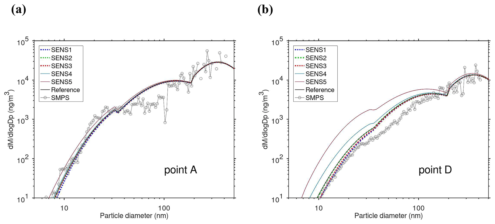
Figure G1Comparison of particle mass size distribution for the diameter range 5–500 nm in the Urban Case simulation. Plots show the modelled mass size distribution from the reference run (including all processes) and the five condensation sensitivity tests (SENS1 to SENS5) with MAFOR together with the observed mass size distribution derived from SMPS measurements using particle density of 1000 kg m−3 to convert from number to mass: (a) size distribution of the total mass at point A; (b) size distribution of the total mass at point D.
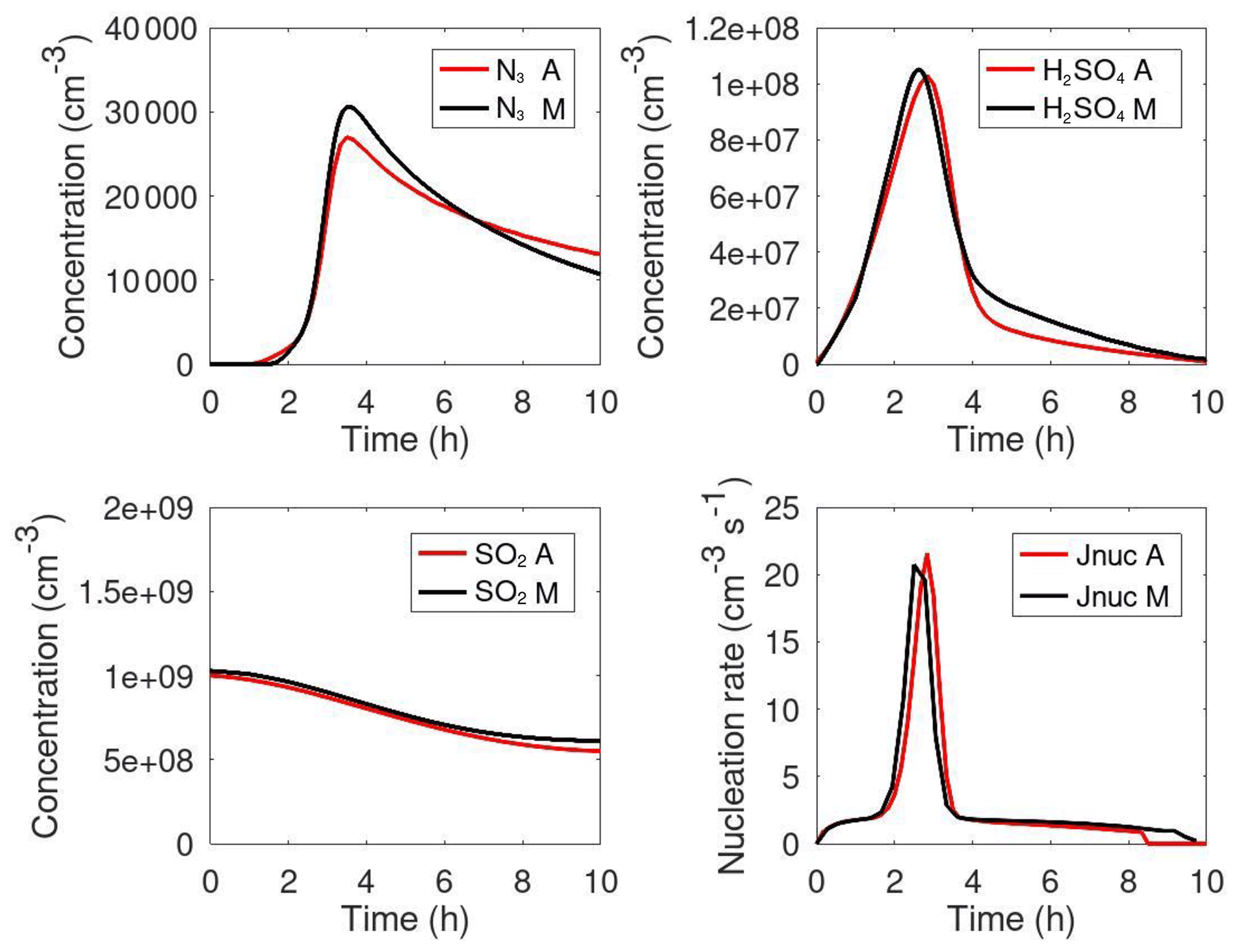
Figure G2Comparison of modelled total particle number with diameter >3 nm (N3), gas-phase concentrations of H2SO4 and SO2, and nucleation rate from MAFOR v2.0 (black lines) and AEROFOR (red lines) in a test of the new nucleation parameterization M2018 for new particle formation under clear-sky conditions (T=267 K, RH =90 %). The simulations started at 8:00 local time.
The modelled mass size distribution obtained in the reference run matches the measured distribution at point A closely, except for the size range 40–100 nm in which the model overestimates measured mass (Fig. G1a), mainly because of inaccurate particle emissions in this size range. Increased volatility of the semi-volatile organics (SENS1) and a lower accommodation coefficient (SENS3) to some extent suppressed the condensation to the sub-10 nm particles. For the sensitivity run with adipic acid (SENS2) no deviation from the reference run is apparent in the mass size distributions. The 20-fold increase in SVOC emissions (SENS4) increases the mass concentrations of sub-10 nm particles at point D (by roughly a factor of 2), but not at point A. The 50-fold increase in SVOC emissions (SENS5) increases mass concentrations of sub-10 nm particles at point A, still consistent with the measured mass size distribution. However, at point D the mass concentrations of particles with diameter <160 nm are largely overestimated compared to the measurements. Given a factor of 2 uncertainty of the experimental mass concentration data (measurement error and uncertain particle density), the emission rate of condensable organics is bound between the reference emission (EF ) as a lower limit and the 20-fold emission (SENS4) as an upper limit for the model to be in agreement with observations. Based on MAFOR simulations, vehicle-emitted organics are thus determined to be on the order of 10−7 to 10−6 .
Particle formation with the new binary parameterization of Määttänen et al. (2018a, b) (M2018) in MAFOR v2.0 was compared against the AEROFOR model in a 10 h simulation experiment with zero background particles (T=267 K and RH = 90 %) under clear-sky conditions. Both models used a size representation with 120 bins in the diameter size range 0.001–1.0 µm. Binary homogeneous neutral and ion-induced nucleation (with an ion pair production rate of 2 cm−3 s−1) using the M2018 code was applied in both models.
New particles were inserted at 1.0 and 1.5 nm diameter in MAFOR and AEROFOR, respectively. Sulfuric acid and an organic vapour were allowed to condense or evaporate with a unity sticking coefficient. The gas-phase concentrations of the OH radical and an organic vapour (C0=0.028 µg m−3) were prescribed by a semisinusoidal pattern. Sulfuric acid formed in the oxidation of SO2 with OH ( cm3 s−1; initial cm−3). Modelled concentrations of OH and H2SO4 peaked at local noon at and cm−3, respectively. The onset of neutral nucleation occurred 2 h after the beginning of the simulation and lasted for about 1 h. Nucleation rate Jnuc peaked at about 21 cm−3 s−1 (Fig. G2). The rate of ion-induced nucleation was almost constant at close to 2 cm−3 s−1 during the experiment. Modelled total number concentrations of particles with diameter >3 nm, N3, reached a maximum 3 h after the beginning of the experiment and dropped afterwards due to decreasing production of sulfuric acid. The radius of critical clusters calculated in the M2018 routine was 0.5 and 0.7 nm for ion-induced and neutral nucleation, respectively, at maximum nucleation. Slight differences are noted between the models in the timing of the nucleation maximum. Maximum N3 calculated in MAFOR (3.1 × 104 cm−3) was 13 % higher than in AEROFOR. The decline of N3 in the second half of the experiment was faster in MAFOR than in AEROFOR, probably due to differences in the parameterization of particle deposition.
The code of the MAFOR v2.0 community model and the relevant data are available at https://doi.org/10.5281/zenodo.5718579 (Karl et al., 2021). This Zenodo repository contains the source code of the MAFOR model as an archived snapshot that was used in this study (including the external libraries for MOSAIC and MECCA), the user manual of the model, and the post-processing scripts applied in the data analysis and model evaluation described in this paper. The model code, documentation, and input data are published under the GPL v3.0. The experimental data measured by the mobile laboratory Sniffer used in this paper can be downloaded from https://doi.org/10.5281/zenodo.5718579 (Karl et al., 2021).
The project repository for the development of the open-source MAFOR v2.0 community model is at https://github.com/mafor2/mafor (last access: 10 May 2022).
A Docker image with the pre-installed MAFOR model based on the official Ubuntu Docker image is available at https://hub.docker.com/repository/docker/matthkarl/ubuntu-mafor2 (last access: 10 May 2022). The image (ca. 1.9 GB) includes the following libraries and programmes: gcc, gfortran-9, gawk, flex, nano, git, graphviz, and octave.
MOSAIC code is accessible within the chemistry version of the Weather Research and Forecasting model (WRF-Chem), which is publicly available. Model users are required to cite Zaveri et al. (2008) in publications resulting from application of MAFOR when the MOSAIC module was activated.
The model code of AEROFOR can be made available upon request to Liisa Pirjola (liisa.pirjola@helsinki.fi) as a private copy. SALSA as a stand-alone model is freely available as an open-source code under the Apache License 2.0. The code is available at https://github.com/UCLALES-SALSA/SALSA-standalone (Kokkola, 2018). For simulating the Urban Case with SALSA, a simple driver was written that models the dispersion and emission of aerosol particles and gases and then calls SALSA functions for aerosol processes. The driver can be found at https://doi.org/10.5281/zenodo.5718579 (Karl et al., 2021).
The supplement related to this article is available online at: https://doi.org/10.5194/gmd-15-3969-2022-supplement.
MaK developed the model code of MAFOR v2, with LP contributing calculation routines for dry deposition and the condensation coefficient, RS supporting the coupling to MECCA, and SJ contributing the ACDC/THN lookup tables. All co-authors participated in developing the concept of the study. JK, MaK, LP, TG, SA, MDM, and MoK designed the setup of the Urban Case simulation. LP prepared the experimental data for the Urban Case. LK did the preprocessing of the meteorological input data. MaK conducted the simulations with MAFOR v2, LK conducted the simulations with AEROFOR, and MoK conducted the simulations with SALSA. SA conducted a simulation with the dispersion–coagulation code LNMOM-DC and discussed results of the particle coagulation experiment. MaK developed the post-processing scripts for the statistical performance analysis. MaK, LP, MoK, and TG analysed the model data for the Urban Case intercomparison. MaK wrote the paper with contributions from all co-authors. JK, LP, SA, AH, DT, and XZ reviewed the paper draft.
At least one of the (co-)authors is a member of the editorial board of Geoscientific Model Development. The peer-review process was guided by an independent editor, and the authors also have no other competing interests to declare.
This work reflects only the authors' view, and the
Innovation and European Climate, Infrastructure and Environment
Executive Agency (CINEA) is not responsible for any use that may
be made of the information it contains. This research has
also received funding from the Academy of Finland for the project
“Global health risks related to atmospheric composition and
weather (GLORIA)”.
Publisher's note: Copernicus Publications remains neutral with regard to jurisdictional claims in published maps and institutional affiliations.
We thank Caroline Leck and Allan Gross for encouraging the publication of MAFOR as an open-source model. We want to thank Martin Seipenbusch (ParteQ GmbH) for permission to use experimental data on particle coagulation experiments. We are grateful to the following contributors for giving permission to publish their codes as part of open-source MAFOR v2: Francis S. Binkowski for the aerosol water uptake routine, Tareq Hussein for the module on dry deposition onto rough surfaces, Anni Määttänen for the new parameterization on sulfuric acid–water nucleation, Joonas Merikanto for the THN code, Hanna Vehkamäki for the BHN code, and Fangqun Yu for the TIMN lookup table code. Rahul A. Zaveri is acknowledged for maintaining the MOSAIC code in WRF-Chem.
This research has been supported by the European Commission Horizon 2020 Framework Programme projects SCIPPER (grant no. 814893) and EMERGE (grant no. 874990).
The article processing charges for this open-access publication were covered by the Helmholtz-Zentrum Hereon.
This paper was edited by Samuel Remy and reviewed by two anonymous referees.
Abdul-Razzak, H. and Ghan, S. J.: A parameterization of aerosol activation, 3. Sectional representation, J. Geophys. Res., 107, 4026, https://doi.org/10.1029/2001JD000483, 2002. a
Adams, P. J. and Seinfeld, J. H.: Predicting global aerosol size distributions in general circulation models, J. Geophys. Res., 107, 4370, https://doi.org/10.1029/2001JD001010, 2002. a
Alam, M. K.: The effect of van der Waals and viscous forces on aerosol coagulation, Aerosol Sci. Technol., 6, 41–52, https://doi.org/10.1080/02786828708959118, 1987. a
Alanen, J., Saukko, E., Lehtoranta, K., Murtonen, T., Timonen, H., Hillamo, R., Karjalainen, P., Kuuluvainen, H., Harra, J., Keskinen, J., and Rönkkö, T.: The formation and physical properties of the particle emissions from a natural gas engine, Fuel, 162, 155–161, https://doi.org/10.1016/j.fuel.2015.09.003, 2015. a, b
Anand, S. and Mayya, Y. S.: Coagulation in a diffusing Gaussian aerosol puff: Comparison of analytical approximations with numerical solutions, J. Aerosol Sci., 40, 348–361, https://doi.org/10.1016/j.jaerosci.2008.12.004, 2009. a
Anand, S. and Mayya, Y. S.: Comment on “Reduced efficacy of marine cloud brightening geoengineering due to in-plume aerosol coagulation: parameterization and global implications” by Stuart et al. (2013), Atmos. Chem. Phys., 15, 753–756, https://doi.org/10.5194/acp-15-753-2015, 2015. a, b, c
Anand, S., Mayya, Y. S., Yu, M., Seipenbusch, M., and Kasper, G.: A numerical study of coagulation of nanoparticle aerosols injected continuously into a large, well stirred chamber, J. Aerosol Sci., 52, 18–32, https://doi.org/10.1016/j.jaerosci.2012.04.010, 2012. a, b
Andersson, C., Bergström, R., Bennet, C., Robertson, L., Thomas, M., Korhonen, H., Lehtinen, K. E. J., and Kokkola, H.: MATCH-SALSA – Multi-scale Atmospheric Transport and CHemistry model coupled to the SALSA aerosol microphysics model– Part 1: Model description and evaluation, Geosci. Model Dev., 8, 171–189, https://doi.org/10.5194/gmd-8-171-2015, 2015. a
Andreae, M. O. and Rosenfeld, D.: Aerosol-cloud-precipitation interactions. Part 1. The nature and sources of cloud-active aerosols, Earth Sci. Rev., 89, 13–41, https://doi.org/10.1016/j.earscirev.2008.03.001, 2008. a
Bakand, S., Hayes, A., and Dechsakulthorn, F.: Nanoparticles: a review of particle toxicology following inhalation exposure, Inhal. Toxicol., 24, 125–135, https://doi.org/10.3109/08958378.2010.642021, 2012. a
Baranizadeh, E., Murphy, B. N., Julin, J., Falahat, S., Reddington, C. L., Arola, A., Ahlm, L., Mikkonen, S., Fountoukis, C., Patoulias, D., Minikin, A., Hamburger, T., Laaksonen, A., Pandis, S. N., Vehkamäki, H., Lehtinen, K. E. J., and Riipinen, I.: Implementation of state-of-the-art ternary new-particle formation scheme to the regional chemical transport model PMCAMx-UF in Europe, Geosci. Model Dev., 9, 2741–2754, https://doi.org/10.5194/gmd-9-2741-2016, 2016. a, b
Bergman, T., Kerminen, V.-M., Korhonen, H., Lehtinen, K. J., Makkonen, R., Arola, A., Mielonen, T., Romakkaniemi, S., Kulmala, M., and Kokkola, H.: Evaluation of the sectional aerosol microphysics module SALSA implementation in ECHAM5-HAM aerosol-climate model, Geosci. Model Dev., 5, 845–868, https://doi.org/10.5194/gmd-5-845-2012, 2012. a
Berkowicz, R., Hertel, O., Sørensen, N. N., and Michelsen, J. A.: Modelling air pollution from traffic in urban areas, in: Flow and dispersion through groups of obstacles, edited by: Perkins, R. J. and Belcher, S. E., Clarendon Press, Oxford, UK, 121–141, ISBN: 0198511906, 1997. a, b
Binkowski, F. and Shankar, U.: The Regional Particulate Matter Model: 1. Model description and preliminary results, J. Geophys. Res., 100, 26191–26209, 1995. a, b
Bolsaitis, P. and Elliott, J. F.: Thermodynamic activities and equilibrium partial pressures for aqueous sulfuric acid solutions, J. Phys. Chem. Eng. Data., 35, 69–85, https://doi.org/10.1021/je00059a022, 1990. a
Bowman, F. M., Odum, J. R., Seinfeld, J. H., and Pandis, S. N.: Mathematical model for gas-particle partitioning of secondary organic aerosols, Atmos. Environ., 31, 3921–3931, https://doi.org/10.1016/S1352-2310(97)00245-8, 1997. a
Boy, M., Hellmuth, O., Korhonen, H., Nilsson, E. D., ReVelle, D., Turnipseed, A., Arnold, F., and Kulmala, M.: MALTE – model to predict new aerosol formation in the lower troposphere, Atmos. Chem. Phys., 6, 4499–4517, https://doi.org/10.5194/acp-6-4499-2006, 2006. a
Breitner, S., Liu, L., Cyrys, J., Brüske, I., Franck, U., Schlink, U., Leitte, A. M., Herbarth, O., Wiedensohler, A., Wehner, B., Hu, M., Pan, X.-C., Wichmann, H.-E., and Peters, A.: Sub-micrometer particulate air pollution and cardiovascular mortality in Beijing, China, Sci. Total Environ., 409, 5196–5204, https://doi.org/10.1016/j.scitotenv.2011.08.023, 2011. a
Capaldo, K. P., Pilinis, C., and Pandis, S.: A computationally efficient hybrid approach for dynamic gas/aerosol transfer in air quality models, Atmos. Environ., 34, 3617–3627, https://doi.org/10.1016/S1352-2310(00)00092-3, 2000. a
Carlton, A. G., Bhave, P. V., Napelenok, S. L., Edney, E. O., Sarwar, G., Pinder, R. W., Pouliot, G. A., and Houyoux, M.: Model representation of secondary organic aerosol in CMAQv4.7, Environ. Sci. Technol., 44, 8553–8560, https://doi.org/10.1021/es100636q, 2010. a
Carslaw, D. C. and Ropkins, K.: openair – an R package for air quality data analysis, Environ. Model. Softw., 27–28, 52–61, https://doi.org/10.1016/j.envsoft.2011.09.008, 2012. a
Chan, C. K., Flagan, R. C., and Seinfeld, J. H.: Water activities of NH4NO3(NH4)2SO4 solutions, Atmos. Environ., 26, 1661–1673, https://doi.org/10.1016/0960-1686(92)90065-S, 1992. a
Chan, T. L., Luo, D. D., Cheung, C. S., Chan, C. K.: Large eddy simulation of flow structures and pollutant dispersion in the near-wake region of the studied ground vehicle for different driving conditions, Atmos. Environ., 42, 5317–5339, https://doi.org/10.1016/j.atmosenv.2008.02.068, 2008. a
Chen, X., Wang, Z., Li, J., Yang, W., Chen, H., Wang, Z., Hao, J., Ge, B., Wang, D., and Huang, H.: Simulation on different response characteristics of aerosol particle number concentration and mass concentration to emission changes over mainland China, Sci. Total Environ., 643, 692–703, https://doi.org/10.1016/j.scitotenv.2018.06.181, 2018. a
Chosson, F., Paoli, R., and Cuenot, B.: Ship plume dispersion rates in convective boundary layers for chemistry models, Atmos. Chem. Phys., 8, 4841–4853, https://doi.org/10.5194/acp-8-4841-2008, 2008. a
DeCarlo, P. F., Slowik, J. G., Worsnop, D. R., Davidovits, P., and Jimenez, J. L.: Particle morphology and density characterization by combined mobility and aerodynamic diameter measurements. Part 1: Theory, Aerosol Sci. Technol., 38, 1185–1205, https://doi.org/10.1080/027868290903907, 2004. a
Donahue, N. M., Robinson, A. L., Stanier, C. O., and Pandis, S. N.: Coupled partitioning, dilution, and chemical aging of semivolatile organics, Environ. Sci. Technol., 40, 2635–2643, https://doi.org/10.1021/es052297c, 2006. a
Donahue, N. M., Epstein, S. A., Pandis, S. N., and Robinson, A. L.: A two-dimensional volatility basis set: 1. organic-aerosol mixing thermodynamics, Atmos. Chem. Phys., 11, 3303–3318, https://doi.org/10.5194/acp-11-3303-2011, 2011. a, b, c, d
Ehn, M., Thornton, J. A., Kleist, E., Sipilä, M., Junninen, H., Pullinen, I., Springer, M., Rubach, F., Tillmann, R., Lee, B., Lopez-Hilfiker, F., Andres, S., Ismail-Hakki, A., Rissanen, M., Jokinen, T., Schobesberger, S., Kangasluoma, J., Kontkanen, J., Nieminen, T., Kurtén, T., Nielsen, L. B., Jørgensen, S., Kjaergaard, H. G., Canagaratna, M., Dal Maso, M., Berndt, T., Petäjä, T., Wahner, A., Kerminen, V.-M., Kulmala, M., Worsnop, D. R., Wildt, J., and Mentel, T. F.: A large source of low-volatility secondary organic aerosol, Nature, 506, 476–479, https://doi.org/10.1038/nature13032, 2014. a
Emerson, E. W., Hodshire, A. L., DeBolt, H. M., Bilsback, K. R., Pierce, J. R., McMeeking, G. R., and Farmer, D. K.: Revisiting particle dry deposition and its role in radiative effect estimates, Proc. Natl. Acad. Sci. USA, 117, 26076–26082, https://doi.org/10.1073/pnas.2014761117, 2020. a
Ervens, B., Feingold, G., Frost, G. J., and Kreidenweis, S. M.: A modeling study of aqueous production of dicarboxylic acids: 1. Chemical pathways and speciated organic mass production, J. Geophys. Res., 109, D15205, https://doi.org/10.1029/2003JD004387, 2004. a
Evans, K. A., Halterman, J. S., Hopke, P. K., Fagnano, M., and Rich, D. Q.: Increased ultrafine particles and carbon monoxide concentrations are associated with asthma exacerbation among urban children, Environ. Res., 129, 11–19, https://doi.org/10.1016/j.envres.2013.12.001, 2014. a
Farren, N. J., Davison, J., Rose, R. A., Wagner, R. L., and Carslaw, D. C.: Underestimated ammonia emissions from road vehicles, Environ. Sci. Technol., 54, 15689–15697, https://doi.org/10.1021/acs.est.0c05839, 2020. a
Fitzgerald, J. W., Hoppel, W. A., and Gelbard, F.: A one-dimensional sectional model to simulate multicomponent aerosol dynamics in the marine boundary layer. 1. Model description, J. Geophys. Res., 103, 16085–16102, https://doi.org/10.1029/98JD01018, 1998. a
Fountoukis, C., Riipinen, I., Denier van der Gon, H. A. C., Charalampidis, P. E., Pilinis, C., Wiedensohler, A., O'Dowd, C., Putaud, J. P., Moerman, M., and Pandis, S. N.: Simulating ultrafine particle formation in Europe using a regional CTM: contribution of primary emissions versus secondary formation to aerosol number concentrations, Atmos. Chem. Phys., 12, 8663–8677, https://doi.org/10.5194/acp-12-8663-2012, 2012. a
Fuchs, N. A.: The Mechanics of Aerosols, edited by: Davies, C. N., translated by: Daisley, R. E. and Fuchs, M., Pergamon Press, London, UK, ISBN: 9780080100661, 1964. a, b
Fuchs, N. A. and Sutugin, A. G.: Highly Dispersed Aerosols, Ann Arbor Science Publ., Ann Arbor, MI, USA, ISBN: 9780706507607, 1970. a, b
Ge, X., Wexler, A. S., and Clegg, S. L.: Atmospheric amines – Part II. Thermodynamic properties and gas/particle partitioning, Atmos. Environ., 45, 561–577, https://doi.org/10.1016/j.atmosenv.2010.10.013, 2011. a
Gelbard, F.: Modeling multicomponent aerosol particle growth by vapor condensation, Aerosol Sci. Technol., 12, 399–412, https://doi.org/10.1080/02786829008959355, 1990. a
Gelbard, F. and Seinfeld, J. H.: Simulation of multicomponent aerosol dynamics, J. Colloid Interface Sci., 78, 485–501, https://doi.org/10.1016/0021-9797(80)90587-1, 1980. a, b
Gidhagen, L., Johansson, C., Ström, J., Kristensson, A., Swietlicki, E., Pirjola, L., and Hansson H.-C.: Model simulation of ultrafine particles inside a road tunnel, Atmos. Environ., 37, 2023–2036, https://doi.org/10.1016/S1352-2310(03)00124-9, 2003. a
Gidhagen, L., Johansson, C., Langner, J., and Olivares, G.: Simulation of NOx and ultrafine particles in a street canyon in Stockholm, Sweden, Atmos. Environ., 38, 2029–2044, https://doi.org/10.1016/j.atmosenv.2004.02.014, 2004. a, b, c
Gidhagen, L., Johansson, C., Langner, J., and Foltescu, V. L.: Urban scale modeling of particle number concentration in Stockholm, Atmos. Environ., 39, 1711–1725, https://doi.org/10.1016/j.atmosenv.2004.11.042, 2005. a
Hamilton, R. S. and Mansfield, T. A.: Airborne particulate elemental carbon: its sources, transport and contribution to dark smoke and soiling, Atmos. Environ., 25A, 715–723, https://doi.org/10.1016/0960-1686(91)90070-N, 1991. a
Harrison, R. M., Jones, A. M., Beddows, D. C. S., Dall'Osto, M., and Nikolova, I.: Evaporation of traffic-generated nanoparticles during advection from source, Atmos. Environ., 125, 1–7, https://doi.org/10.1016/j.atmosenv.2015.10.077, 2016. a
Henschel, H., Kurtén, T., and Vehkamäki, H.: Computational study on the effect of hydration on new particle formation in the sulfuric acid/ammonia and sulphuric acid/dimethylamine systems, J. Phys. Chem. A, 120, 1886–1896, https://doi.org/10.1021/acs.jpca.5b11366, 2016. a
Hietikko, R., Kuuluvainen, H., Harrison, R. M., Portin, H., Timonen, H., Niemi, J. V., and Rönkkö, T.: Diurnal variation of nanocluster aerosol concentrations and emission factors in a street canyon, Atmos. Environ., 189, 98–106, https://doi.org/10.1016/j.atmosenv.2018.06.031, 2018. a
Hussein, T., Smolik, J., Kerminen, V.-M., and Kulmala, M.: Modeling dry deposition of aerosol particles onto rough surfaces, Aerosol Sci. Technol., 46, 44–59, https://doi.org/10.1080/02786826.2011.605814, 2012. a, b
Hyvärinen, A.-P., Lihavainen, H., Gaman, A., Vairila, L., Ojala, H., Kulmala, M. and Viisanen, Y.: Surface tensions and densities of oxalic, malonic, succinic, maleic, malic, and cis-pinonic acids, J. Chem. Eng. Data 51, 255–260, https://doi.org/10.1021/je050366x, 2006. a
Jacobson, M. Z.: Development and application of a new air pollution modeling system – II. Aerosol module structure and design, Atmos. Environ., 31, 131–144, https://doi.org/10.1016/1352-2310(96)00202-6, 1997a. a
Jacobson, M. Z.: Numerical techniques to solve condensational and dissolutional growth equations when growth is coupled to reversible reactions, Aerosol Sci. Technol., 27, 491–498, https://doi.org/10.1080/02786829708965489, 1997b. a, b, c
Jacobson, M. Z.: Studying the effects of calcium and magnesium on size-distributed nitrate and ammonium with EQUISOLV II, Atmos. Environ., 33, 3635–3649, https://doi.org/10.1016/S1352-2310(99)00105-3, 1999. a
Jacobson, M. Z.: A solution to the problem of nonequilibrium acid/base gas-particle transfer at long time step, Aerosol Sci. Technol., 39, 92–103, https://doi.org/10.1080/027868290904546, 2005a. a, b, c, d, e, f, g
Jacobson, M. Z.: Fundamentals of Atmospheric Modeling, 2nd edn., Cambridge University Press, Cambridge, UK, ISBN: 0521548659, 2005b. a, b, c, d, e, f, g, h, i, j
Jacobson, M. Z. and Seinfeld, J. H.: Evolution of nanoparticle size and mixing state near the point of emission, Atmos. Environ., 38, 1839–1850, https://doi.org/10.1016/j.atmosenv.2004.01.014, 2004. a, b, c, d
Jacobson, M. Z. and Turco, R. P.: Simulating condensational growth, evaporation, and coagulation of aerosols using a combined moving and stationary size grid, Aerosol Sci. Technol., 22, 73–92, https://doi.org/10.1080/02786829408959729, 1995. a, b
Jacobson, M. Z., Kittelson, D. B., and Watts, W. F.: Enhanced coagulation due to evaporation and its effect on nanoparticle evolution. Environ. Sci. Technol., 39, 9486–9492, https://doi.org/10.1021/es0500299, 2005. a
Jaecker-Voirol, A., Mirabel, P. and Reiss, H.: Hydrates in supersaturated binary sulfuric acid-water vapor: a re-examination, J. Chem. Phys. 87, 4849–4852, https://doi.org/10.1063/1.452847, 1987. a
Järvinen, A., Timonen, H., Karjalainen, P., Bloss, M., Simonen, P., Saarikoski, S., Kuuluvainen, H., Kalliokoski, J., Dal Maso, M., Niemi, J. V., Keskinen, J., and Rönkkö, T.: Particle emissions of Euro VI, EEV and retrofitted EEV city buses in real traffic, Environ. Pollut., 250, 708–716, https://doi.org/10.1016/j.envpol.2019.04.033, 2019. a
Julin, J., Winkler, P. M., Donahue, N. M., Wagner, P. E., and Riipinen, I.: Near-unity mass accommodation coefficient of organic molecules of varying structure, Environ. Sci. Technol., 48, 12083–12089, https://doi.org/10.1021/es501816h, 2014. a
Kangasniemi, O., Kuuluvainen, H., Heikkilä, J., Pirjola, L., Niemi, J. V., Timonen, H., Saarikoski, S., Rönkkö, T., and Dal Maso, M.: Dispersion of a traffic related nanocluster aerosol near a major road, Atmosphere, 10, 309, https://doi.org/10.3390/atmos10060309, 2019. a
Karl, M., Gross, A., Leck, C., and Pirjola, L.: Intercomparison of dimethylsulfide oxidation mechanisms for the marine boundary layer: gaseous and particulate sulfur constituents, J. Geophys. Res., 112, D15304, https://doi.org/10.1029/2006JD007914, 2007. a, b
Karl, M., Gross, A., Pirjola, L., and Leck, C.: A new flexible multicomponent model for the study of aerosol dynamics in the marine boundary layer, Tellus B, 63, 1001–1025, https://doi.org/10.1111/j.1600-0889.2011.00562.x, 2011. a, b, c, d, e, f, g, h, i
Karl, M., Leck, C., Gross, A., and Pirjola, L.: A study of new particle formation in the marine boundary layer over the central Arctic Ocean using a flexible multicomponent aerosol dynamic model, Tellus B, 64, 17158, https://doi.org/10.3402/tellusb.v64i0.17158, 2012a. a, b, c
Karl, M., Dye, C., Schmidbauer, N., Wisthaler, A., Mikoviny, T., D'Anna, B., Müller, M., Borrás, E., Clemente, E., Muñoz, A., Porras, R., Ródenas, M., Vázquez, M., and Brauers, T.: Study of OH-initiated degradation of 2-aminoethanol, Atmos. Chem. Phys., 12, 1881–1901, https://doi.org/10.5194/acp-12-1881-2012, 2012b. a, b, c, d
Karl, M., Leck, C., Coz, E., and Heintzenberg, J.: Marine nanogels as a source of atmospheric nanoparticles in the high Arctic, Geophys. Res. Lett., 40, 3738–3743, https://doi.org/10.1002/grl.50661, 2013. a, b
Karl, M., Kukkonen, J., Keuken, M. P., Lützenkirchen, S., Pirjola, L., and Hussein, T.: Modeling and measurements of urban aerosol processes on the neighborhood scale in Rotterdam, Oslo and Helsinki, Atmos. Chem. Phys., 16, 4817–4835, https://doi.org/10.5194/acp-16-4817-2016, 2016. a, b, c, d, e, f, g, h
Karl, M., Walker, S.-E., Solberg, S., and Ramacher, M. O. P.: The Eulerian urban dispersion model EPISODE – Part 2: Extensions to the source dispersion and photochemistry for EPISODE–CityChem v1.2 and its application to the city of Hamburg, Geosci. Model Dev., 12, 3357–3399, https://doi.org/10.5194/gmd-12-3357-2019, 2019. a, b, c, d
Karl, M., Pirjola, L., Karppinen, A., Jalkanen, J.-P., Ramacher, M. O. P., and Kukkonen, J.: Modeling of the concentrations of ultrafine particles in the plumes of ships in the vicinity of major harbors, Int. J. Environ. Res. Public Health, 17, 777, https://doi.org/10.3390/ijerph17030777, 2020. a, b, c
Karl, M., Pirjola, L., Grönholm, T., Kurppa, M., Anand, S., Zhang, X., Held, A., Sander, R., Dal Maso, M., Topping, D., Jiang, S., Kangas, L., and Kukkonen, J.: Release of the community aerosol dynamics model MAFOR v2 and the urban case dataset published in Karl et al., GMD, (v1.9.9), Zenodo [code], https://doi.org/10.5281/zenodo.5718580, 2021. a, b, c
Karppinen, A., Kukkonen, J., Elolähde, T., Konttinen, M., Koskentalo, T., and Rantakrans, E.: A modelling system for predicting urban air pollution: Model description and applications in the Helsinki metropolitan area, Atmos. Environ., 34, 3723–3733, https://doi.org/10.1016/S1352-2310(00)00074-1, 2000. a
Kerminen, V.-M., Mäkelä, T. E., Ojanen, C. H., Hillamo, R. E., Vilhunen, J. K., Rantanen, L., Havers, N., von Bohlen, A., and Klockow, D.: Characterization of the particulate phase in the exhaust from a diesel car, Environ. Sci. Technol., 31, 1883–1889, https://doi.org/10.1021/es960520n, 1997. a, b, c
Kerminen, V.-M., Pakkanen, T. A., Mäkelä, T., Hillamo, R. E., Rönkkö, T., Virtanen, A., Keskinen, J., Pirjola, L., Hussein, T., and Hämeri, K.: Development of particle number size distribution near a major road in Helsinki during an episodic inversion situation, Atmos. Environ., 41, 1759–1767, https://doi.org/10.1016/j.atmosenv.2006.10.026, 2007. a
Ketzel, M. and Berkowicz, R.: Modelling the fate of ultrafine particles from exhaust pipe to rural background: An analysis of time scales for dilution, coagulation and deposition, Atmos. Environ., 38, 2639–2652, https://doi.org/10.1016/j.atmosenv.2004.02.020, 2004. a, b, c, d, e
Keuken, M. P., Henzing, J. S., Zandveld, P., van den Elshout, S., and Karl, M.: Dispersion of particle numbers and elemental carbon from road traffic, a harbor and an airstrip in the Netherlands, Atmos. Environ., 54, 320–327, https://doi.org/10.1016/j.atmosenv.2012.01.012, 2012. a, b
Keuken, M. P., Moerman, M., Zandveld, P., and Henzing, J. S.: Total and size-resolved particle number and black carbon concentrations near an industrial area, Atmos. Environ., 122, 196–205, https://doi.org/10.1016/j.atmosenv.2015.01.015, 2015. a
Kokkola, H.: UCLALES-SALSA/SALSA-standalone 2.0 (v2.0), Zenodo [code], https://doi.org/10.5281/zenodo.1251669, 2018. a
Kokkola, H., Korhonen, H., Lehtinen, K. E. J., Makkonen, R., Asmi, A., Järvenoja, S., Anttila, T., Partanen, A.-I., Kulmala, M., Järvinen, H., Laaksonen, A., and Kerminen, V.-M.: SALSA – a Sectional Aerosol module for Large Scale Applications, Atmos. Chem. Phys., 8, 2469–2483, https://doi.org/10.5194/acp-8-2469-2008, 2008. a, b, c, d
Kokkola, H., Kühn, T., Laakso, A., Bergman, T., Lehtinen, K. E. J., Mielonen, T., Arola, A., Stadtler, S., Korhonen, H., Ferrachat, S., Lohmann, U., Neubauer, D., Tegen, I., Siegenthaler-Le Drian, C., Schultz, M. G., Bey, I., Stier, P., Daskalakis, N., Heald, C. L., and Romakkaniemi, S.: SALSA2.0: The sectional aerosol module of the aerosol–chemistry–climate model ECHAM6.3.0-HAM2.3-MOZ1.0, Geosci. Model Dev., 11, 3833–3863, https://doi.org/10.5194/gmd-11-3833-2018, 2018. a
Korhonen, H., Lehtinen, K. E. J., and Kulmala, M.: Multicomponent aerosol dynamics model UHMA: model development and validation, Atmos. Chem. Phys., 4, 757–771, https://doi.org/10.5194/acp-4-757-2004, 2004. a, b, c, d, e, f
Kouznetsov, R. and Sofiev, M.: A methodology for evaluation of vertical dispersion and dry deposition of atmospheric aerosols, J. Geophys. Res., 117, 1–19, https://doi.org/10.1029/2011JD016366, 2012. a
Kreidenweis, S. M. and Seinfeld, J. H.: Nucleation of sulfuric acid-water and methanesulfonic acid-water solution particles: Implications for the atmospheric chemistry of organosulfur species, Atmos. Environ., 22, 283–296, https://doi.org/10.1016/0004-6981(88)90034-0, 1988. a
Kukkonen, J., Olsson, T., Schultz, D. M., Baklanov, A., Klein, T., Miranda, A. I., Monteiro, A., Hirtl, M., Tarvainen, V., Boy, M., Peuch, V.-H., Poupkou, A., Kioutsioukis, I., Finardi, S., Sofiev, M., Sokhi, R., Lehtinen, K. E. J., Karatzas, K., San José, R., Astitha, M., Kallos, G., Schaap, M., Reimer, E., Jakobs, H., and Eben, K.: A review of operational, regional-scale, chemical weather forecasting models in Europe, Atmos. Chem. Phys., 12, 1–87, https://doi.org/10.5194/acp-12-1-2012, 2012. a
Kukkonen, J., Karl, M., Keuken, M. P., Denier van der Gon, H. A. C., Denby, B. R., Singh, V., Douros, J., Manders, A., Samaras, Z., Moussiopoulos, N., Jonkers, S., Aarnio, M., Karppinen, A., Kangas, L., Lützenkirchen, S., Petäjä, T., Vouitsis, I., and Sokhi, R. S.: Modelling the dispersion of particle numbers in five European cities, Geosci. Model Dev., 9, 451–478, https://doi.org/10.5194/gmd-9-451-2016, 2016. a, b, c, d
Kukkonen, J., Kangas, L., Kauhaniemi, M., Sofiev, M., Aarnio, M., Jaakkola, J. J. K., Kousa, A., and Karppinen, A.: Modelling of the urban concentrations of PM2.5 on a high resolution for a period of 35 years, for the assessment of lifetime exposure and health effects, Atmos. Chem. Phys., 18, 8041–8064, https://doi.org/10.5194/acp-18-8041-2018, 2018. a, b
Kulmala, M., Pirjola, L., and Mäkelä, J. M.: Stable sulphate clusters as a source of new atmospheric particles, Nature, 404, 66–69, https://doi.org/10.1038/35003550, 2000. a
Kulmala, M., Vehkamäki, H., Petäjä, T., Dal Maso, M., Lauri, A., Kerminen, V.-M., Birmili, W., and McMurry, P. H.: Formation and growth rates of ultrafine atmospheric particles: a review of observations, J. Aerosol Sci., 35, 143–176, https://doi.org/10.1016/j.jaerosci.2003.10.003, 2004. a
Kulmala, M., Lehtinen, K. E. J., and Laaksonen, A.: Cluster activation theory as an explanation of the linear dependence between formation rate of 3 nm particles and sulphuric acid concentration, Atmos. Chem. Phys., 6, 787–793, https://doi.org/10.5194/acp-6-787-2006, 2006. a, b, c, d
Kumar, P., Fennell, P., Langley, D., and Britter, R.: Pseudo-simultaneous measurements for the vertical variation of coarse, fine and ultrafine particles in an urban street canyon, Atmos. Environ., 42, 4304–4319, https://doi.org/10.1016/j.atmosenv.2008.01.010, 2008. a
Kumar, P., Robins, A., and Britter, R.: Fast response measurements for the dispersion of nanoparticles in a vehicle wake and in a street canyon, Atmos. Environ., 43, 6110–6118, https://doi.org/10.1016/j.atmosenv.2009.08.042, 2009. a
Kumar, P., Ketzel, M., Vardoulakis, S., Pirjola, L., and Britter, R.: Dynamics and dispersion modelling of nanoparticles from road traffic in the urban atmospheric environment – A review, J. Aerosol Sci., 42, 580–603, https://doi.org/10.1016/j.jaerosci.2011.06.001, 2011. a, b, c, d, e
Kurppa, M., Hellsten, A., Roldin, P., Kokkola, H., Tonttila, J., Auvinen, M., Kent, C., Kumar, P., Maronga, B., and Järvi, L.: Implementation of the sectional aerosol module SALSA2.0 into the PALM model system 6.0: model development and first evaluation, Geosci. Model Dev., 12, 1403–1422, https://doi.org/10.5194/gmd-12-1403-2019, 2019. a, b, c, d
Kurppa, M., Roldin, P., Strömberg, J., Balling, A., Karttunen, S., Kuuluvainen, H., Niemi, J. V., Pirjola, L., Rönkkö, T., Timonen, H., Hellsten, A., and Järvi, L.: Sensitivity of spatial aerosol particle distributions to the boundary conditions in the PALM model system 6.0, Geosci. Model Dev., 13, 5663–5685, https://doi.org/10.5194/gmd-13-5663-2020, 2020. a, b, c
Lambe, A. T., Miracolo, M. A., Hennigan, C. J., Robinson, A. L., and Donahue, N. M.: Effective rate constants and uptake coefficients for the reactions of organic molecular markers (n-alkanes, hopanes, and steranes) in motor oil and diesel primary organic aerosols with hydroxyl radicals, Environ. Sci. Technol., 43, 8794–8800, https://doi.org/10.1021/es901745h, 2009. a
Landgraf, J. and Crutzen, P. J.: An efficient method for online calculations of photolysis and heating rates, J. Atmos. Sci., 55, 863–878, https://doi.org/10.1175/1520-0469(1998)055<0863:AEMFOC>2.0.CO;2, 1998. a
Lee, Y. H. and Adams, P. J.: Evaluation of aerosol distributions in the GISS-TOMAS global aerosol microphysics model with remote sensing observations, Atmos. Chem. Phys., 10, 2129–2144, https://doi.org/10.5194/acp-10-2129-2010, 2010. a
Legates, D. R. and McCabe, G. J.: Evaluating the use of “goodness-of-fit” Measures in hydrologic and hydroclimatic model validation, Water Resour. Res., 35, 233–241, https://doi.org/10.1029/1998WR900018, 1999. a
Lehtinen, K. E. J. and Kulmala, M.: A model for particle formation and growth in the atmosphere with molecular resolution in size, Atmos. Chem. Phys., 3, 251–257, https://doi.org/10.5194/acp-3-251-2003, 2003. a
Lemmetty, M., Pirjola, L., Mäkelä, J. M., Rönkkö, T., and Keskinen, J.: Computation of maximum rate of water-sulphuric acid nucleation in diesel exhaust, J. Aerosol Sci., 37, 1596–1604, https://doi.org/10.1016/j.jaerosci.2006.04.003, 2006. a
Lemmetty, M., Rönkkö, T., Virtanen, A., Keskinen, J. and Pirjola, L.: The Effect of Sulphur in Diesel Exhaust Aerosol: Models Compared with Measurements, Aerosol Sci. Technol., 42, 11916–11929, https://doi.org/10.1080/02786820802360682, 2008. a
Lim, Y. B. and Ziemann, P. J.: Effects of molecular structure on aerosol yields from OH radical-initiated reactions of linear, branched, and cyclic alkanes in the presence of NOx, Environ. Sci. Technol., 43, 2328–2334, https://doi.org/10.1021/es100636q, 2009. a
LIPASTO: Calculation system for traffic exhaust emissions and energy use in Finland, VTT Technical Research Centre of Finland Ltd., http://lipasto.vtt.fi/en/index.htm, last access: 8 November 2021. a
Määttänen, A., Merikanto, J., Henschel, H., Duplissy, J., Makkonen, R., Ortega, I. K., and Vehkamäki, H.: New parameterizations for neutral and ion-induced sulfuric acid-water particle formation in nucleation and kinetic regimes, J. Geophys. Res.-Atmos., 123, 1269–1296, https://doi.org/10.1002/2017JD027429, 2018a. a, b, c, d
Määttänen, A., Merikanto, J., Henschel, H., Duplissy, J., Makkonen, R., Ortega, I. K., and Vehkamäki, H.: Revised release of a Fortran code including the particle formation parameterizations published in Määttänen et al., JGR D, 2018 (v1.0, Vol. 123, pp. 1269–1296), J. Geophys. Res.-Atmos., Zenodo [code], https://doi.org/10.5281/zenodo.1217782, 2018b. a, b
Mallik, C., Tomsche, L., Bourtsoukidis, E., Crowley, J. N., Derstroff, B., Fischer, H., Hafermann, S., Hüser, I., Javed, U., Keßel, S., Lelieveld, J., Martinez, M., Meusel, H., Novelli, A., Phillips, G. J., Pozzer, A., Reiffs, A., Sander, R., Taraborrelli, D., Sauvage, C., Schuladen, J., Su, H., Williams, J., and Harder, H.: Oxidation processes in the eastern Mediterranean atmosphere: evidence from the modelling of HOx measurements over Cyprus, Atmos. Chem. Phys., 18, 10825–10847, https://doi.org/10.5194/acp-18-10825-2018, 2018. a
Maricq, M. M., Xu, N., and Chase, R. E.: Measuring particulate mass emissions with the Electrical Low Pressure Impactor, Aerosol Sci. Technol., 40, 68–79, https://doi.org/10.1080/02786820500466591, 2006. a
Mårtensson, E. M., Nilsson, E. D., de Leeuw, G., Cohen, L. H., and Hansson, H.-C.: Laboratory simulations and parameterization of the primary marine aerosol production, J. Geophys. Res., 108, 4297, https://doi.org/10.1029/2002JD002263, 2003. a
Mauritsen, T., Sedlar, J., Tjernström, M., Leck, C., Martin, M., Shupe, M., Sjogren, S., Sierau, B., Persson, P. O. G., Brooks, I. M., and Swietlicki, E.: An Arctic CCN-limited cloud-aerosol regime, Atmos. Chem. Phys., 11, 165–173, https://doi.org/10.5194/acp-11-165-2011, 2011. a
McGraw, R.: Description of aerosol dynamics by the quadrature method of moments, Aerosol Sci. Technol., 27, 255–265, https://doi.org/10.1080/02786829708965471, 1997. a
Merikanto, J., Napari, I., Vehkamäki, H., Anttila, T., and Kulmala, M.: New parameterization of sulphuric acid-ammonia-water ternary nucleation rates at tropospheric conditions, J. Geophys. Res., 112, 1–9, https://doi.org/10.1029/2006JD007977, 2007. a, b
Merikanto, J., Napari, I., Vehkamäki, H., Anttila, T., and Kulmala, M.: Correction to “New parameterization of sulphuric acid-ammonia-water ternary nucleation rates at tropospheric conditions”, J. Geophys. Res., 114, 1–2, https://doi.org/10.1029/2009JD012136, 2009. a
Meskhidze, N., Jaimes-Correa, J. C., Petters, M. D., Royalty, T. M., Phillips, B. N., Zimmerman, A., and Reed, R.: Possible wintertime sources of fine particles in an urban environment, J. Geophys. Res.-Atmos., 124,, 13055–13070, https://doi.org/10.1029/2019JD031367, 2019. a
Morawska, L., Ristovski, Z., Jayaratne, E. R., Koegh, D. U., and Ling, X.: Ambient nano and ultrafine particles from motor vehicle emissions: characteristics, ambient processing and implications on human exposure, Atmos. Environ., 42, 8113–8138, https://doi.org/10.1016/j.atmosenv.2008.07.050, 2008. a
Meng, Z. and Seinfeld, J. H.: Time scales to achieve gas-aerosol equilibrium for volatile species, Atmos. Environ., 30, 2889–2900, https://doi.org/10.1016/1352-2310(95)00493-9, 1996.
Metzger, A., Verheggen, B., Dommen, J., Duplissy, J., Prevôt, A. S., Weingartner, E., Riipinen, I., Kulmala, M., Spracklen, D. V., Carslaw, K. S., and Baltensperger, U.: Evidence for the role of organics in aerosol particle formation under atmospheric conditions, P. Natl. Acad. Sci., 107, 6646–6651, https://doi.org/10.1073/pnas.0911330107, 2010. a
Monahan, E. C., Spiel, D. E., and Davidson, K. L.: A model of marine aerosol generation via whitecaps and wave disruption, in: Oceanic Whitecaps, 1st edn., Oceanographic Sciences Library, edited by: Monahan, E. C. and Mac Niocaill, G., 167–174, D. Reidel, Norwell, Massachusetts, ISBN: 9789027722515, 1986. a
Napari, I., Noppel, M., Vehkamäki, H., and Kulmala, M.: An improved model for ternary nucleation of sulfuric-acid-ammonia water, J. Chem. Phys., 116, 4221–4227, https://doi.org/10.1063/1.1450557, 2002. a
Nenes, A., Pandis, S. N., and Pilinis, C.: Continued development and testing of a new thermodynamic aerosol module for urban and regional air quality models, Atmos. Environ., 33, 1553–1560, https://doi.org/10.1016/S1352-2310(98)00352-5, 1999. a
Nielsen, C. J., D'Anna, B., Karl, M., Aursnes, M., Boreave, A., Bossi, R., Bunkan, A. J. C., Glasius, M., Hallquist, M., Hansen, A.-M. K., Kristensen, K., Mikoviny, T., Maguta, M. M., Müller, M., Nguyen, Q., Westerlund, J., Salo, K., Skov, H., Stenstrøm, Y., and Wisthaler, A.: Atmospheric Degradation of Amines. Summary Report: Photo-oxidation of methylamine, dimethylamine and trimethylamine, CLIMIT project no. 201604, NILU Report OR 2/2011, Norwegian Institute for Air Research, Kjeller, Norway, https://www.nilu.com/publication/25495/ (last access: 9 May 2022), 2011. a
Nikolova, I., Janssen, S., Vos, P., and Berghmans, P.: Modelling the mixing of size resolved traffic induced and background ultrafine particles from an urban street canyon to adjacent backyards, Aerosol Air Qual. Res., 14, 145–155, https://doi.org/10.4209/aaqr.2013.06.0221, 2014. a, b
Noppel, M., Vehkamäki, H., and Kulmala, M.: An improved model for hydrate formation in sulfuric acid-water nucleation, J. Chem. Phys., 116, 218–228, https://doi.org/10.1063/1.1423333, 2002. a
Olenius, T., Kupiainen-Määttä, O., Ortega, I. K., Kurtén, T., and Vehkamäki, H.: Free energy barrier in the growth of sulphuric acid–ammonia and sulfuric acid–dimethylamine clusters, J. Chem. Phys., 139, 084312, https://doi.org/10.1063/1.4819024, 2013. a
Olin, M., Kuuluvainen, H., Aurela, M., Kalliokoski, J., Kuittinen, N., Isotalo, M., Timonen, H. J., Niemi, J. V., Rönkkö, T., and Dal Maso, M.: Traffic-originated nanocluster emission exceeds H2SO4-driven photochemical new particle formation in an urban area, Atmos. Chem. Phys., 20, 1–13, https://doi.org/10.5194/acp-20-1-2020, 2020. a
Paasonen, P., Nieminen, T., Asmi, E., Manninen, H. E., Petäjä, T., Plass-Dülmer, C., Flentje, H., Birmili, W., Wiedensohler, A., Hõrrak, U., Metzger, A., Hamed, A., Laaksonen, A., Facchini, M. C., Kerminen, V.-M., and Kulmala, M.: On the roles of sulphuric acid and low-volatility organic vapours in the initial steps of atmospheric new particle formation, Atmos. Chem. Phys., 10, 11223–11242, https://doi.org/10.5194/acp-10-11223-2010, 2010. a, b, c, d
Paasonen, P., Kupiainen, K., Klimont, Z., Visschedijk, A., Denier van der Gon, H. A. C., and Amann, M.: Continental anthropogenic primary particle number emissions, Atmos. Chem. Phys., 16, 6823–6840, https://doi.org/10.5194/acp-16-6823-2016, 2016. a
Peng, C. and Chan, C. K.: The water cycles of water-soluble organic salts of atmospheric importance, Atmos. Environ., 35, 1183–1192, https://doi.org/10.1016/S1352-2310(00)00426-X ,2001. a
Petersen, W. B.: User's Guide for Hiway-2: A Highway Air Pollution Model, US Environmental Protection Agency, EPA-600/8-80-018, Research Triangle Park, NC, USA, https://nepis.epa.gov (last access: 8 November 2021), 1980. a
Petroff, A., Mailliat, A., Amielh, M., and Anselmet, F.: Aerosol dry deposition on vegetative canopies. Part II: A new modelling approach and applications, Atmos. Environ., 42, 3654–3683, https://doi.org/10.1016/j.atmosenv.2007.12.060, 2008. a
Petters, M. D. and Kreidenweis, S. M.: A single parameter representation of hygroscopic growth and cloud condensation nucleus activity, Atmos. Chem. Phys., 7, 1961–1971, https://doi.org/10.5194/acp-7-1961-2007, 2007. a
Pierce, J., Theodoritsi, G., Adams, P., and Pandis, S. N.: Parameterization of the effect of sub-grid scale aerosol dynamics on aerosol number emission rates, J. Aerosol Sci., 40, 385–393, https://doi.org/10.1016/j.jaerosci.2008.11.009, 2009. a
Pirjola, L.: Effects of the increased UV radiation and biogenic VOC emissions on ultrafine sulphate aerosol formation, J. Aerosol Sci., 3, 355–367, https://doi.org/10.1016/S0021-8502(98)00065-2, 1999. a, b
Pirjola, L. and Kulmala, M.: Modelling the formation of H2SO4-H2O particles in rural, urban and marine conditions, Atmos. Res., 46, 321–347, https://doi.org/10.1016/S0169-8095(97)00072-0, 1998. a
Pirjola, L. and Kulmala, M.: Development of particle size and composition distributions with a novel aerosol dynamics model, Tellus B, 53, 491–509, https://doi.org/10.3402/tellusb.v53i4.17128, 2001. a, b, c
Pirjola, L., Laaksonen, A., Aalto, P., and Kulmala, M.: Sulfate aerosol formation in the Arctic boundary layer, J. Geophys. Res., 103, 8309–8321, https://doi.org/10.1029/97JD03079, 1998. a, b
Pirjola, L., O'Dowd, C. D. and Kulmala, M.: A model prediction of the yield of CCN from tidal-related nucleation events, J. Geophys. Res., 107, PAR3-1–PAR3-15, https://doi.org/10.1029/2000JD000213, 2002. a
Pirjola, L., Tsyro, S., Tarrason, L., and Kulmala, M.: A monodisperse aerosol dynamics module – a promising candidate for use in the Eulerian long-range transport model, J. Geophys. Res., 108, 4258, https://doi.org/10.1029/2002JD002867, 2003. a
Pirjola, L., Lehtinen, K. E. J., Hansson, H.-C., and Kulmala, M.: How important is nucleation in regional/global modelling, Geophys. Res. Lett., 31, L12109, 1–4, https://doi.org/10.1029/2004GL019525, 2004. a
Pirjola, L., Lähde, T., Niemi, J. V., Kousa, A., Rönkkö, T., Karjalainen, P., Keskinen, J., Frey, A., and Hillamo, R.: Spatial and temporal characterization of traffic emissions in urban microenvironments with a mobile laboratory, Atmos. Environ., 63, 156–167, https://doi.org/10.1016/j.atmosenv.2012.09.022, 2012. a, b, c, d, e, f
Pirjola, L., Pajunoja, A., Walden, J., Jalkanen, J.-P., Rönkkö, T., Kousa, A., and Koskentalo, T.: Mobile measurements of ship emissions in two harbour areas in Finland, Atmos. Meas. Tech., 7, 149–161, https://doi.org/10.5194/amt-7-149-2014, 2014. a
Pirjola, L., Karl, M., Rönkkö, T., and Arnold, F.: Model studies of volatile diesel exhaust particle formation: are organic vapours involved in nucleation and growth?, Atmos. Chem. Phys., 15, 10435–10452, https://doi.org/10.5194/acp-15-10435-2015, 2015. a, b, c, d, e
Pnueli, D., Gutfinger, C., and Fichman, M.: A turbulent-Brownian model for aerosol coagulation, Aerosol Sci. Technol., 14, 201–209, https://doi.org/10.1080/02786829108959483, 1991. a
Pohjola, M. A., Pirjola, L., Kukkonen, J., and Kulmala, M.: Modelling of the influence of aerosol processes for the dispersion of vehicular exhaust plumes in street environment, Atmos. Environ., 37, 339–351, https://doi.org/10.1016/S1352-2310(02)00887-7, 2003. a
Pohjola, M. A., Pirjola, L., Karppinen, A., Härkönen, J., Korhonen, H., Hussein, T., Ketzel, M., and Kukkonen, J.: Evaluation and modelling of the size fractionated aerosol particle number concentration measurements nearby a major road in Helsinki – Part I: Modelling results within the LIPIKA project, Atmos. Chem. Phys., 7, 4065–4080, https://doi.org/10.5194/acp-7-4065-2007, 2007. a, b, c, d, e, f, g, h, i, j
Pringle, K. J., Tost, H., Message, S., Steil, B., Giannadaki, D., Nenes, A., Fountoukis, C., Stier, P., Vignati, E., and Lelieveld, J.: Description and evaluation of GMXe: a new aerosol submodel for global simulations (v1), Geosci. Model Dev., 3, 391–412, https://doi.org/10.5194/gmd-3-391-2010, 2010. a
Pruppacher, H. R. and Klett, J. D.: Microphysics of Clouds and Precipitation, 2nd edn., Kluwer Academic Publishers, Dordrecht, The Netherlands, 954 pp., ISBN: 0-79-234211-1, 1997. a
Reid, R. C., Prausnitz, J. M., and Poling, B. E.: The Properties of Gases and Liquids, 4th edn., edited by: Sun, B. and Fleck, G. H., McGraw-Hill, New York, USA, 741 pp., ISBN: 0070517991, 1987. a
Riemer, N., West, M., Zaveri, R. A., and Easter, R. C.: Simulating the evolution of soot mixing state with a particle-resolved aerosol model, J. Geophys. Res., 114, 1–22, https://doi.org/10.1029/2008JD011073, 2009. a, b
Rivas, I., Beddows, D. C. S., Amato, F., Green, D. C., Järvi, L., Hueglin, C., Reche, C., Timonen, H., Fuller, G. W., Niemi, J. V., Pérez, N., Aurela, M., Hopke, P. K., Alastuey, A., Kulmala, M., Harrison, R. M., Querol, X., and Kelly, F. J.: Source apportionment of particle number size distribution in urban background and traffic stations in four European cities, Environ. Int., 135, 1–19, https://doi.org/10.1016/j.envint.2019.105345, 2020. a
Rogak, S. N. and Flagan, R. C.: Coagulation of aerosol agglomerates in the transition regime, J. Colloid Interface Sci., 151, 203–224, https://doi.org/10.1016/0021-9797(92)90252-H, 1992. a
Roldin, P., Swietlicki, E., Schurgers, G., Arneth, A., Lehtinen, K. E. J., Boy, M., and Kulmala, M.: Development and evaluation of the aerosol dynamics and gas phase chemistry model ADCHEM, Atmos. Chem. Phys., 11, 5867–5896, https://doi.org/10.5194/acp-11-5867-2011, 2011. a, b, c
Rönkkö, T., Virtanen, A., Kannosto, J., Keskinen, J., Lappi, M., and Pirjola, L.: Nucleation mode particles with a non-volatile core in the exhaust of a heavy duty diesel vehicle, Environ. Sci. Technol., 41, 6384–6389, https://doi.org/10.1021/es0705339, 2007. a
Rönkkö, T., Lähde, T., Heikkilä, J., Pirjola, L., Bauschke, U., Arnold, F., Schlager, H., Rothe, D., Yli-Ojanperä, J., and Keskinen, J.: Effects of gaseous sulphuric acid on diesel exhaust nanoparticle formation and characteristics, Environ. Sci. Technol., 47, 11882–11889, 2013. a
Rönkkö, T., Kuuluvainen, H., Karjalainen, P., Keskinen, J., Hillamo, R., Niemi, J. V., Pirjola, L., Timonen, H. J., Saarikoski, S., Saukko, E., Järvinen, A., Silvennoinen, H., Rostedt, A., Olin, M., Yli-Ojanperä, J., Nousiainen, P., Kousa, A., Dal Maso, M.: Traffic is a major source of atmospheric nanocluster aerosol, Proc. Natl. Acad. Sci. USA, 114, 7549–7554, https://doi.org/10.1073/pnas.1700830114, 2017. a
Salo, L., Mylläri, F., Maasikmets, M., Niemelä, V., Konist, A., Vainumäe, K., Kupri, H.-L., Titova, R., Simonen, P., Aurela, M., Bloss, M., Keskinen, J., Timonen, H., and Rönkkö, T.: Emission measurements with gravimetric impactors and electrical devices: An aerosol instrument comparison, Aerosol Sci. Technol., 53, 526–539, https://doi.org/10.1080/02786826.2019.1578858, 2019. a
Sander, S. P., Abbatt, J., Barker, J. R., Burkholder, J. B., Friedl, R. R., Golden, D. M., Huie, R. E., Kolb, C. E., Kurylo, M. J., Moortgat, G. K., Orkin, V. L., and Wine, P. H.: Chemical Kinetics and Photochemical Data for Use in Atmospheric Studies, Evaluation No. 17, JPL Publication 10-6, Jet Propulsion Laboratory, Pasadena, https://jpldataeval.jpl.nasa.gov/pdf/JPL%2010-6%20Final%2015June2011.pdf (last access: 8 November 2021), 2011. a
Sander, R., Jöckel, P., Kirner, O., Kunert, A. T., Landgraf, J., and Pozzer, A.: The photolysis module JVAL-14, compatible with the MESSy standard, and the JVal PreProcessor (JVPP), Geosci. Model Dev., 7, 2653–2662, https://doi.org/10.5194/gmd-7-2653-2014, 2014. a, b
Sander, R., Baumgaertner, A., Cabrera-Perez, D., Frank, F., Gromov, S., Grooß, J.-U., Harder, H., Huijnen, V., Jöckel, P., Karydis, V. A., Niemeyer, K. E., Pozzer, A., Riede, H., Schultz, M. G., Taraborrelli, D., and Tauer, S.: The community atmospheric chemistry box model CAABA/MECCA-4.0, Geosci. Model Dev., 12, 1365–1385, https://doi.org/10.5194/gmd-12-1365-2019, 2019. a, b
Sandu, A. and Sander, R.: Technical note: Simulating chemical systems in Fortran90 and Matlab with the Kinetic PreProcessor KPP-2.1, Atmos. Chem. Phys., 6, 187–195, https://doi.org/10.5194/acp-6-187-2006, 2006. a
Sarkar, T., Anand, S., Singh, K. D., Tripathi, R. M., Pradeepkumar, K. S., Goto, D., and Nakajima, T. :Simulating long range transport of radioactive aerosols using a global aerosol transport model, Aerosol Air Qual. Res., 17, 2631–2642, https://doi.org/10.4209/aaqr.2017.01.0049, 2017. a
Sarkar, T., Anand, S., Singh, K. D., Kulkarni, M. S., Mayya, Y. S., and Venkataraman, C.: Near-source aerosol dynamics – a parameterization scheme for global aerosol transport model, European Aerosol Conference (EAC 2020), Aachen, Germany, 31 August–4 September 2020, https://phaidra.univie.ac.at/view/o:1164483 (last access: 10 May 2022), 2020. a, b, c
Schack Jr., C. J., Pratsinis, S. E., and Friedlander, S. K.: A general correlation for deposition of suspended particles from turbulent gases to completely rough surfaces, Atmos. Environ., 19, 953–960, https://doi.org/10.1016/0004-6981(85)90240-9, 1985. a, b
Schmitt-Ott, A. and Burtscher, H.: The effect of van der Waals forces on aerosol coagulation, J. Colloid Interface Sci., 89, 353–357, https://doi.org/10.1016/0021-9797(82)90187-4, 1982. a
Schwartz S. E.: Mass transport considerations pertinent to aqueous phase reactions of gases in liquid water clouds, in: Chemistry of Multiphase Atmospheric Systems, NATO ASI Series, Vol. 6, edited by: Jaeschke, W., Springer, Berlin, 415–471, https://doi.org/10.1007/978-3-642-70627-1_16, 1986. a
Seinfeld, J. H. and Pandis, S. N.: Atmospheric Chemistry and Physics: From Air Pollution to Climate Change, 2nd edn., Wiley-Interscience, Hoboken, NJ, USA, ISBN: 9780471720188, 2006. a
Sihto, S.-L., Kulmala, M., Kerminen, V.-M., Dal Maso, M., Petäjä, T., Riipinen, I., Korhonen, H., Arnold, F., Janson, R., Boy, M., Laaksonen, A., and Lehtinen, K. E. J.: Atmospheric sulphuric acid and aerosol formation: implications from atmospheric measurements for nucleation and early growth mechanisms, Atmos. Chem. Phys., 6, 4079–4091, https://doi.org/10.5194/acp-6-4079-2006, 2006. a
Simpson, D.: Long-period modelling of photochemical oxidants in Europe. Model calculations for July 1985, Atmos. Environ., 26, 1609–1634, 1992. a
Singh, V., Sokhi, R., and Kukkonen, J.: PM2.5 concentrations in London for 2008 – A modeling analysis of contributions from road traffic, JAPCA J. Air. Waste Ma., 64, 509–518, https://doi.org/10.1080/10962247.2013.848244, 2014. a
Smith, M. H., Park, P. M., and Consterdine, I. E.: Marine aerosol concentrations and estimated fluxes over the sea, Q. J. Roy. Meteor. Soc., 119, 809–824, https://doi.org/10.1002/qj.49711951211, 1993. a
Spada, M., Jorba, O., Pérez García-Pando, C., Janjic, Z., and Baldasano, J. M.: Modeling and evaluation of the global sea-salt aerosol distribution: sensitivity to size-resolved and sea-surface temperature dependent emission schemes, Atmos. Chem. Phys., 13, 11735–11755, https://doi.org/10.5194/acp-13-11735-2013, 2013. a, b
Spracklen, D. V., Pringle, K. J., Carslaw, K. S., Chipperfield, M. P., and Mann, G. W.: A global off-line model of size-resolved aerosol microphysics: I. Model development and prediction of aerosol properties, Atmos. Chem. Phys., 5, 2227–2252, https://doi.org/10.5194/acp-5-2227-2005, 2005. a
Stier, P., Feichter, J., Kinne, S., Kloster, S., Vignati, E., Wilson, J., Ganzeveld, L., Tegen, I., Werner, M., Balkanski, Y., Schulz, M., Boucher, O., Minikin, A., and Petzold, A.: The aerosol-climate model ECHAM5-HAM, Atmos. Chem. Phys., 5, 1125–1156, https://doi.org/10.5194/acp-5-1125-2005, 2005. a
Tang, I. N. and Munkelwitz, H. R.: Water activities, densities, and refractive indices of aqueous sulfates and sodium nitrate droplets of atmospheric importance, J. Geophys. Res., 99, 18801–18808, https://doi.org/10.1029/94JD01345, 1994. a
Tang, I. N., Tridico, A. C., and Fung, K. H.: Thermodynamic and optical properties of sea salt aerosols, J. Geophys. Res., 102, 23269–23275, https://doi.org/10.1029/97JD01806, 1997. a
Tian, J., Riemer, N., West, M., Pfaffenberger, L., Schlager, H., and Petzold, A.: Modeling the evolution of aerosol particles in a ship plume using PartMC-MOSAIC, Atmos. Chem. Phys., 14, 5327–5347, https://doi.org/10.5194/acp-14-5327-2014, 2014. a
Tonttila, J., Maalick, Z., Raatikainen, T., Kokkola, H., Kühn, T., and Romakkaniemi, S.: UCLALES–SALSA v1.0: a large-eddy model with interactive sectional microphysics for aerosol, clouds and precipitation, Geosci. Model Dev., 10, 169–188, https://doi.org/10.5194/gmd-10-169-2017, 2017. a, b
Tsang, T. H. and Rao, A.: Comparison of different numerical schemes for condensational growth of aerosols, Aerosol Sci. Technol., 9, 271–277, https://doi.org/10.1080/02786828808959214, 1988. a
Tsimpidi, A. P., Karydis, V. A., Zavala, M., Lei, W., Molina, L., Ulbrich, I. M., Jimenez, J. L., and Pandis, S. N.: Evaluation of the volatility basis-set approach for the simulation of organic aerosol formation in the Mexico City metropolitan area, Atmos. Chem. Phys., 10, 525–546, https://doi.org/10.5194/acp-10-525-2010, 2010. a
Tzivion, S., Feingold, G., and Levin, Z.: An efficient numerical-solution to the stochastic collection equation, J. Atmos. Sci., 44, 3139–3149, 1987. a
Vardoulakis, S., Fisher, B. E. A., Pericleous, K., and Gonzalez-Flesca, N.: Modelling air quality in street canyons: a review, Atmos. Environ., 37, 155–182, https://doi.org/10.1016/S1352-2310(02)00857-9, 2003. a
Vehkamäki, H., Kulmala, M., Napari, I., Lehtinen, K. E. J., Timmreck, C., Noppel, M., and Laaksonen, A.: An improved parameterization for sulfuric acid-water nucleation rates for tropospheric and stratospheric conditions, J. Geophys. Res., 107, 4622, AAC3-1–AAC3-10, https://doi.org/10.1029/2002JD002184, 2002. a, b
Vehkamäki, H., Kulmala, M., Lehtinen, K. E. J., and Noppel, M.: Modelling binary homogeneous nucleation of water-sulfuric acid vapours: Parameterisation for high temperature emissions, Environ. Sci. Technol., 37, 3392–3398, https://doi.org/10.1021/es0263442, 2003. a, b
Vignati, E., Berkowicz, R., Palmgren, F., Lyck, E., and Hummelshoj, P.: Transformation of size distributions of emitted particles in streets, Sci. Total Environ., 235, 37–49, https://doi.org/10.1016/S0048-9697(99)00188-6, 1999. a, b, c, d, e
Vignati, E., Wilson, J., and Stier, P.: M7 – An efficient size-resolved aerosol microphysics module for large-scale aerosol transport models, J. Geophys. Res., 109, D22202, https://doi.org/10.1029/2003JD004485, 2004. a, b
Wang, M., Chen, D., Xiao, M., Ye, Q., Stolzenburg, D., Hofbauer, V., Ye, P., Vogel, A. L., Mauldin III, R. L., Amorim, A., Baccarini, A., Baumgartner, B., Brilke, S., Dada, L., Dias, A., Duplissy, J., Finkenzeller, H., Garmash, O., He, X.-C., Hoyle, C. R., Kim, C., Kvashnin, A., Lehtipalo, K., Fischer, L., Molteni, U., Petäjä, T., Pospisilova, V., Quéléver, L. L. J., Rissanen, M., Simon, M., Tauber, C., Tomé, A., Wagner, A. C., Weitz, L., Volkamer, R., Winkler, P. M., Kirkby, J., Worsnop, D. R., Kulmala, M., Baltensperger, U., Dommen, J., El-Haddad, I., and Donahue, N. M.: Photo-oxidation of aromatic hydrocarbons produces low-volatility organic compounds, Environ. Sci. Technol., 54, 7911–7921, https://doi.org/10.1021/acs.est.0c02100, 2020. a
Warren, D. R. and Seinfeld, J. H.: Simulation of aerosol size distribution evolution in systems with simultaneous nucleation, condensation, and coagulation, Aerosol Sci. Technol., 4, 31–43, https://doi.org/10.1080/02786828508959037, 1985. a
Weber, R. J., McMurry, P. H., Mauldin, R. L., Tanner, D., Eisele, F. L., Clarke, A. D., and Kapustin, V.: New particle formation in the remote troposphere: A comparison of observations at various sites, Geophys. Res. Lett., 26, 307–310, https://doi.org/10.1029/1998GL900308, 1999. a
Wexler, A. S. and Clegg, S. L.: Atmospheric aerosol models for systems including the ions H+, , Na+, , , Cl−, Br−, and H2O, J. Geophys. Res., 107, 4207, https://doi.org/10.1029/2001JD000451, 2002. a
Whitby, E. R. and McMurry, P. H.: Modal aerosol dynamics modeling, Aerosol Sci. Technol., 27, 673–688, https://doi.org/10.1080/02786829708965504, 1997. a
Wichmann, H. E. and Peters, A.: Epidemiological evidence of the effects of ultrafine particle exposure, Philos. Trans. Royal Soc. A, 358, 2751–2769, https://doi.org/10.1098/rsta.2000.0682, 2000. a
Willmott, C. J., Robeson, S. M., and Matsuura, K.: A refined index of model performance, Int. J. Climatol., 32, 2088–2094, https://doi.org/10.1002/joc.2419, 2012. a, b
Wright, D. L., Kasibhatla, P. S., McGraw, R., and Schwartz, S. E.: Description and evaluation of a six-moment aerosol microphysical module for use in atmospheric chemical transport models, J. Geophys. Res., 106, 20275–20291, https://doi.org/10.1029/2001JD900098, 2001. a
Wyslouzil, B. E., Seinfeld, J. H., Flagan, R. C., and Okuyama, K.: Binary nucleation in acid-water systems – Part 1: methanesulfonic acid-water, J. Chem. Phys., 94, 6827–6841, https://doi.org/10.1063/1.460261, 1991. a
Yu, F. and Turco, R. P.: From molecular clusters to nanoparticles: Role of ambient ionization in tropospheric aerosol formation, J. Geophys. Res., 106, 4797–4814, https://doi.org/10.1029/2000JD900539, 2001. a
Yu, F., Nadykto, A. B., Herb, J., Luo, G., Nazarenko, K. M., and Uvarova, L. A.: H2SO4–H2O–NH3 ternary ion-mediated nucleation (TIMN): kinetic-based model and comparison with CLOUD measurements, Atmos. Chem. Phys., 18, 17451–17474, https://doi.org/10.5194/acp-18-17451-2018, 2018. a
Yu, F., Nadykto, A. B., Luo, G., and Herb, J.: H2SO4–H2O binary and H2SO4–H2O–NH3 ternary homogeneous and ion-mediated nucleation: lookup tables version 1.0 for 3-D modeling application, Geosci. Model Dev., 13, 2663–2670, https://doi.org/10.5194/gmd-13-2663-2020, 2020. a, b
Zaveri, R. A., Easter, R. C., and Wexler, A. S.: A new method for multicomponent activity coefficients of electrolytes in aqueous atmospheric aerosols, J. Geophys. Res., 110, D02201, https://doi.org/10.1029/2004JD004681, 2005a. a
Zaveri, R. A., Easter, R. C., and Peter, L. K.: A computationally efficient Multicomponent Equilibrium Solver for Aerosols (MESA), J. Geophys. Res., 110, D24203, https://doi.org/10.1029/2004JD005618, 2005b. a, b, c
Zaveri, R. A., Easter, R. C., Fast, J. D., and Peters, L. K.: Model for Simulating Aerosol Interaction and Chemistry (MOSAIC), J. Geophys. Res., 113, D13204, https://doi.org/10.1029/2007JD008782, 2008. a, b, c
Zhang, K. M. and Wexler, A. S.: Evolution of particle number distribution near roadways – Part I: Analysis of aerosol dynamics and its implications for engine emission measurement, Atmos. Environ., 38, 6643–6653, https://doi.org/10.1016/j.atmosenv.2004.06.043, 2004. a
Zhang, L., Gong, S., Padro, J., and Barrie, L.: A size-segregated particle dry deposition scheme for an atmospheric aerosol module, Atmos. Environ., 35, 549–560, https://doi.org/10.1016/S1352-2310(00)00326-5, 2001. a, b, c
Zhang, R., Khalizov, A. F., Pagels, J., Zhang, D., Xue, H., and McMurry, P. H.: Variability in morphology, hygroscopicity, and optical properties of soot particles during atmospheric processing, Proc. Natl. Acad. Sci. USA, 105, 10291–10296, https://doi.org/10.1073/pnas.0804860105, 2008. a
Zhang, R., Khalizov, A., Wang, L., Hu, M., and Xu, W.: Nucleation and growth of nanoparticles in the atmosphere, Chem. Rev., 112, 1957–2011, https://doi.org/10.1021/cr2001756, 2012. a
Zhang, X., Karl, M., Zhang, L., and Wang, J.: Influence of aviation emission on the particle number concentration near Zurich Airport, Environ. Sci. Technol., 54, 14161–14171, https://doi.org/10.1021/acs.est.0c02249, 2020. a, b
Zhang, Y., Easter, R. C., Ghan, S. J., and Abdul-Razzak, H.: Impact of aerosol size representation on modeling aerosol-cloud interactions, J. Geophys. Res., 107, 4558, https://doi.org/10.1029/2001JD001549, 2002. a
Zhong, J., Nikolova, I., Cai, X., MacKenzie, A. R., Alam, M. S., Xu, R., Singh, A., and Harrison, R. M.: Traffic-induced multicomponent ultrafine particle microphysics in the WRF v3.6.1 large eddy simulation model: General behaviour from idealised scenarios at the neighbourhood-scale, Atmos. Environ., 223, 117213, https://doi.org/10.1016/j.atmosenv.2019.117213, 2020. a
- Abstract
- Introduction
- Model description
- Methods of evaluation against experimental data
- Results
- Summary and conclusions
- Appendix A: List of acronyms and nomenclature
- Appendix B: Analytical Predictor of Condensation
- Appendix C: Brownian coagulation
- Appendix D: Correction factors for the coagulation rate
- Appendix E: Dilution function for the Urban Case
- Appendix F: Statistical indicators and model performance indicators
- Appendix G: Comparison of modelled and measured mass size distributions
- Appendix H: Performance of the implemented nucleation code M2018
- Code and data availability
- Author contributions
- Competing interests
- Disclaimer
- Acknowledgements
- Financial support
- Review statement
- References
- Supplement