the Creative Commons Attribution 4.0 License.
the Creative Commons Attribution 4.0 License.
 | 16 May 2022
Description of historical and future projection simulations by the global coupled E3SMv1.0 model as used in CMIP6
Tian Zhou
Luke P. Van Roekel
Jean-Christophe Golaz
Hailong Wang
Philip Cameron-Smith
This paper documents the experimental setup and general features of the coupled historical and future climate simulations with the first version of the US Department of Energy (DOE) Energy Exascale Earth System Model (E3SMv1.0). The future projected climate characteristics of E3SMv1.0 at the highest emission scenario (SSP5-8.5) designed in the Scenario Model Intercomparison Project (ScenarioMIP) and the SSP5-8.5 greenhouse gas (GHG) only forcing experiment are analyzed with a focus on regional responses of atmosphere, ocean, sea ice, and land.
Due to its high equilibrium climate sensitivity (ECS of 5.3 K), E3SMv1.0 is one of the Coupled Model Intercomparison Project phase 6 (CMIP6) models with the largest surface warming by the end of the 21st century under the high-emission SSP5-8.5 scenario. The global mean precipitation change is highly correlated with the global temperature change, while the spatial pattern of the change in runoff is consistent with the precipitation changes. The oceanic mixed layer generally shoals throughout the global ocean. The annual mean Atlantic meridional overturning circulation (AMOC) is overly weak with a slower change from ∼ 11 to ∼ 6 Sv (Sverdrup) relative to other CMIP6 models. The sea ice, especially in the Northern Hemisphere, decreases rapidly with large seasonal variability. We detect a significant polar amplification in E3SMv1.0 from the atmosphere, ocean, and sea ice.
Comparing the SSP5-8.5 all-forcing experiment with the GHG-only experiment, we find that the unmasking of the aerosol effects due to the decline of the aerosol loading in the future projection period causes transient accelerated warming in the all-forcing experiment in the first half of the 21st century. While the oceanic climate response is mainly controlled by the GHG forcing, the land runoff response is impacted primarily by forcings other than GHG over certain regions, e.g., southern North America, southern Africa, central Africa, and eastern Asia. However, the importance of the GHG forcing on the land runoff changes grows in the future climate projection period compared to the historical period.
- Article
(27303 KB) - Full-text XML
- BibTeX
- EndNote


Compared to previous Coupled Model Intercomparison Project phase 6 (CMIP6) climate models, the latest CMIP phase 6 (CMIP6) models simulate a higher ensemble equilibrium climate sensitivity (ECS) with a larger spread (Meehl et al., 2020; Zelinka et al., 2020). Within CMIP6, the Scenario Model Intercomparison Project (ScenarioMIP) aims to generate multi-model climate projections for alternate scenarios of future emissions and land-use changes produced with integrated assessment models. The climate model projections from the ScenarioMIP experiments facilitate scientific understandings of future climate change. An ensemble analysis of the Scenario-MIP participating global coupled Earth system models has shown that the global mean surface air temperature and surface precipitation response of each individual model is highly correlated with its climate sensitivity, especially for the high-emission scenario (Tebaldi et al., 2021).
The US Department of Energy (DOE) Energy Exascale Earth System Model (E3SM) project is a new and ongoing climate modeling effort to develop a state-of-the-art Earth system model. The E3SM project aims to develop code optimized for DOE's high-performance computing infrastructure and to advance Earth system prediction of changes in environmental variables that are critical to energy-sector decisions, such as regional trends in air and water temperatures, water availability, storms and heavy precipitation, coastal flooding, and sea-level rise (Bader et al., 2014; Leung et al., 2020). E3SM version 1.0 (E3SMv1.0) at the standard horizontal resolution of ∼ 100 km reported a high ECS of 5.3 K, a high transient climate response (TCR) of 2.93 K, along with a strong aerosol-related effective radiative forcing (ERFaero) of −1.65 W m−2 (Golaz et al., 2019). Previous estimates found that the net positive cloud feedback of 0.94 W m−2 K−1 in E3SMv1.0 is too strong compared with other CMIP6 models at the range of 0.42±0.36 W m−2 K−1 (Zelinka et al., 2020, Table S1). The overly high ECS and strong ERFaero resulted in a delayed warming followed by an excessive warming trend during the second half of the 20th century in the E3SMv1.0 historical ensemble (Golaz et al., 2019). It is expected that E3SMv1.0 will be among the warmest models in terms of the global mean surface temperature in future climate projections due to its high ECS and TCR. Through our participation in the ScenarioMIP project, we conducted future climate projection experiments in a high-emission scenario with E3SMv1.0. Inspired by the Detection and Attribution MIP (DAMIP) project (Gillett et al., 2016), we additionally conducted a set of historical and future projection simulations with greenhouse gas (GHG)-only forcing for the high-emission scenario to estimate the contribution of the GHG emissions to observed global warming and the future projected climate change in E3SMv1.0.
There are two main goals for this paper. Firstly, document future climate characteristics of E3SMv1.0 (which is a model member of the ScenarioMIP project) at the highest emission scenario along with its historical climate evolution. In particular, we describe regional responses of key climate components, namely atmosphere, ocean, sea ice, and land runoff in the high-emission scenario simulated by E3SMv1.0. The currently available ScenarioMIP simulations from other CMIP6 models serve as a reference to characterize the E3SMv1.0 simulations. Secondly, we describe regional responses of key climate components in the GHG-only simulations. The difference between the high-emission all-forcing experiment and the GHG-only experiment is analyzed. Specifically, we compare the relative impacts of GHG forcing vs. other forcing on the different climate components. In Sect. 2, we present a brief model description of E3SMv1.0 and the detailed experimental setup. Section 3 includes all the results from these experiments, while the findings are summarized in Sect. 4.
2.1 E3SMv1.0 model description
Golaz et al. (2019) and references therein provide the full description of E3SMv1.0. Here, we only briefly describe the model information relevant to this study. E3SMv1.0 includes five Earth system components (atmosphere, ocean, sea ice, land, and rivers) and the coupler to interface these five components. The atmosphere component of E3SMv1.0, EAMv1, uses a spectral element dynamical core at 110 km resolution on a cubed-sphere geometry. It has 72 layers with a top at approximately 60 km. The main atmosphere physics time step is 30 min. The ocean and sea-ice components of E3SMv1.0 are developed based on the Model for Prediction Across Scales (MPAS) framework (Ringler et al., 2010): MPAS-Ocean and MPAS-Seaice. The MPAS framework uses spherical centroidal Voronoi tessellations (SCVTs) for multi-resolution modeling. MPAS-Ocean and MPAS-Seaice share the same unstructured grid with a horizontal grid spacing varying from 30 km in the tropics and high latitudes to 60 km in the midlatitudes. The vertical discretization consists of 60 layers with thickness varying from 10 m at the surface to 250 m at depth. Ocean model time step is 10 min with a barotropic sub-time step of 40 s. The sea-ice model time step is 30 min. The land component in E3SMv1.0, ELMv1, is developed from the Community Land Model version 4.5. The time step of ELMv1 is 30 min. The river runoff component of E3SMv1.0 is the Model for Scale Adaptive River Transport (MOSART). In the standard E3SMv1.0 1∘ resolution, MOSART uses a regular latitude–longitude grid with the resolution of 0.5∘. The time step of MOSART is 1 h. The component coupler in E3SMv1.0 is the Common Infrastructure for Modeling the Earth. The coupling frequency for all components is 30 min, except for MOSART which communicates every 3 h.
The key source code git hash numbers involved in the E3SMv1.0 simulation campaign are documented in Golaz et al. (2019). A maintenance branch (maint-1.0; https://github.com/E3SM-Project/E3SM/tree/maint-1.0, last access: 12 May 2022) has also been created and maintained to reproduce these E3SMv1.0 simulations performed for this study. The run scripts used to set up simulations beyond the default configuration in the model compset and submit jobs for these experiments are also archived to reproduce these simulations (see “Code availability”).
2.2 The CMIP6 historical experiment
The E3SMv1.0 CMIP6 historical simulations follow the CMIP6 Diagnosis, Evaluation, and Characterization of Klima (DECK) specifications (Eyring et al., 2016). Golaz et al. (2019) documents the model input data (i.e., input4MIPS data), the spin-up, initialization, and the tuning efforts for the E3SMv1.0 pre-industrial control simulation (piControl). Five ensemble members of the CMIP6 historical simulations (historical_Hn) were initialized from 1 January of five different years of the piControl simulation (Golaz et al., 2019, Table 2). These historical_Hn simulations cover the 1850–2014 period.
2.3 ScenarioMIP SSP5-8.5 experiment
The E3SMv1.0 future climate projections adopt the Shared Socioeconomic Pathway – Representative Concentration Pathway (SSP-RCP) framework of the ScenarioMIP experiments (O'Neill et al., 2016). The ScenarioMIP experimental design includes a set of eight pathways of future emissions, concentrations, and land use, with additional ensemble members and long-term extensions to facilitate future research on mitigation, adaptation, and residual climate impacts (O'Neill et al., 2016). We conducted the future climate projection experiment with the high-emission SSP5-8.5 scenario, which represents the upper end of the scenarios in terms of fossil fuel use, food demand, energy use, and greenhouse gas emissions (Kriegler et al., 2017). The high-level results from these future projection runs were included in the CMIP6 ScenarioMIP paper (Tebaldi et al., 2021). The SSP5-8.5 scenario experiment produces a radiative forcing of 8.5 W m−2 in the year 2100 (O'Neill et al., 2016). The relatively high forcing level reached by this scenario enables the model to simulate the potential responses of the Earth system components over a range of global average radiative forcing and temperature changes that are larger than in lower emission scenarios by the end of the 21st century.
Kriegler et al. (2017) describe forcings including global spatial distributions of emissions and concentrations of greenhouse gases, ozone concentrations, aerosols, land use, and other natural forcings, in particular solar forcing and volcanic emissions, for the ScenarioMIP SSP5-8.5 experiment. To keep the consistency through the harmonization of emissions, concentrations, and land use across scenarios and between the SSP5-8.5 simulations and historical simulations, five ensemble members of the ScenarioMIP simulations (future_Pn-SSP5-8.5) use the conditions at the end of the historical_Hn simulations (31 December 2014) as the initial conditions for future climate projections. The E3SM future climate simulations and the CMIP6 historical simulations are performed with the same model configuration, including the input data processing for GHGs and aerosol emissions (Golaz et al., 2019). We will link these two experiments and analyze the present-day climate and the future climate projections together to see if these are any disruptions in the first years of the SSP5-8.5 simulations related to the historical simulations.
2.4 GHG-only experiment
As one of the CMIP6-endorsed MIPs, DAMIP aims to estimate the contributions of anthropogenic and natural forcing changes to observed global warming as well as to observed global and regional changes in other climate variables (Gillett et al., 2016). While there are a number of experimental designs covering the historical period and the future projection period with the SSP2-4.5 future scenario in DAMIP, we simply adopt the “only” approach for the GHG forcing in the historical period and the SSP5-8.5 future scenario. We conducted a total of three ensemble members of the GHG-only simulations for the historical period and the future projection period, respectively. The model settings of these GHG-only historical simulations (historical_Hn-GHG) are the same as those of the historical_Hn runs except that all forcings other than GHG forcing are held at pre-industrial values. The GHG-only future projection simulations (future_Pn-SSP5-8.5-GHG) use the end of the historical_Hn simulations as the starting points and use the GHG forcing in the SSP5-8.5 scenario, while the other forcings are still set at the same pre-industrial values as historical_Hn-GHG. Similarly to the CMIP6 historical experiment and the ScenarioMIP SSP5-8.5 experiment, we connect the GHG-only historical and future projection experiments together to analyze the climate responses from the year 1850 to the year 2099.
3.1 Historical simulation and SSP5-8.5 experiment
3.1.1 Atmosphere climatology
Before we analyze the global mean or zonal mean of the variables, the monthly variables are regridded to 1∘ lat–long grids with the first-order conservative remapping method through NetCDF Operators (NCO) version 4.8.1. CMIP6 models project an overall higher warming with a larger intermodel spread for different forcing levels, particularly for the high-emission SSP5-8.5 scenario, compared to the corresponding CMIP5 future climate projections (e.g., Meehl et al., 2020; Brunner et al., 2020; Tebaldi et al., 2021). These changes are likely due to the different experimental designs between CMIP5 and CMIP6 experiments and the higher climate sensitivities in a subset of the CMIP6 models (Tebaldi et al., 2021). To adopt the CMIP6 models as the reference, this study analyzes these CMIP6 model runs of which both the historical simulation and SSP5-8.5 simulation are available at the time of writing. Only one ensemble member (r1i1p1f1) of the CMIP6 model runs is included in this study.
Figure 1 presents the time evolution of annual global mean near-surface air temperature (Tair) anomalies and surface precipitation rate anomalies with respect to 1850–1869 from E3SMv1.0 along with the other CMIP6 models. As shown in Golaz et al. (2019), E3SMv1.0 simulated global mean Tair anomalies during the historical period demonstrate a prolonged cooling after 1950 and then a rapid warming around 2000. E3SMv1.0 is at the lower end of the model range during the prolonged cooling period (Fig. 1a). However, the Tair anomalies in E3SMv1.0 catch up and reach the middle range of the CMIP6 model spread by the end of the historical run (year 2014) due to the rapid warming. This rapid warming in E3SMv1.0 continues in the SSP5-8.5 experiment at a speed faster than that of most of CMIP6 models. Near the end of the 21st century, E3SMv1.0 projects one of the warmest Tair anomalies at ∼8 K, consistent with the overly strong TCR and ECS. The global mean precipitation rate is driven by the energy balance between the radiative cooling and the latent heating (O'Gorman et al., 2012); the global mean change in precipitation is mainly set by the Clausius–Clapeyron relation as an approximately 7 % K−1 increase in atmospheric water vapor content (e.g., Stephens and Hu, 2010). As a result, the time evolution of the global mean surface precipitation rate (Fig. 1b) is strongly correlated with the Tair trend with larger interannual fluctuations. The median and mean values of the Pearson correlation coefficients for Tair and precipitation anomalies from the CMIP6 models and the E3SMv1.0 simulations are higher than 0.96. The global mean precipitation in E3SMv1.0 increases by >0.3 mm d−1 from the end of the historical period (year 2014) to the end of the future projection (year 2099). The spread of the E3SMv1.0 ensemble members is much smaller than the CMIP6 intermodel spread throughout the historical and future climate projection periods for both Tair and surface precipitation rate anomalies. Treating the available CMIP6 models as a reference, we sort the global mean Tair changes between the years 2070–2099 and 1850–1869 in the SSP5-8.5 simulations from the available CMIP6 models (blue bars) and E3SMv1.0 ensemble members (red bars) from the lowest warming to the highest warming (Fig. 1c). The global mean Tair changes in the E3SMv1.0 ensemble members are comparable to the CMIP6 models with the highest warming.

Figure 1Time evolution of (a) annual global mean near-surface air temperature (Tair) anomalies and (b) annual global mean surface precipitation rate anomalies with respect to 1850–1869 from E3SMv1.0 ensemble members (black lines) and CMIP6 models (colored lines) for the historical simulation and SSP5-8.5 all-forcing experiment. These three ensemble members of the E3SMv1.0 GHG-only experiments are denoted as dashed gray lines. The magenta line in panel (a) is the time series of the observation (HadCRUT4, Morice et al., 2012), while it is the time series of Global Precipitation Climatology Project (GPCP) v2.3 precipitation (Adler et al., 2018) change from the year 1979. (c) The changes of global mean (Tair) from the years 1850–1869 to 2070–2099 for CMIP6 models (blue bars) and the five E3SMv1.0 members from the SSP5-8.5 simulations. The five models between two vertical brown lines and the five models between vertical gray lines are models within 0–20th and 40–60th percentiles, respectively.
The global distribution of the Tair and surface precipitation change in E3SMv1.0 resembles the ensemble average pattern from the ScenarioMIP participant models for the SSP5-8.5 scenario (Tebaldi et al., 2021) based on the global maps of Tair (Fig. 2e) and surface precipitation rate (Fig. 3e) for the years 2070–2099 from the SSP5-8.5 simulations and those for the years 1985–2014 from the historical simulations. The global pattern of Tair change between 2070–2099 and 1985–2014 reveals a polar amplification of surface warming and interhemispheric asymmetric warming. Along the same latitude bands, the surface warming over the continents is generally higher than that of the ocean. The strongest surface warming occurs over the Arctic with a magnitude >15 ∘C.
Figure 2Annual mean Tair (∘C) from (a) five SSP5.85 ensemble simulations (2070-2099), (c) five historical ensemble simulations (1985–2014), and (e) the change between the time period of 2070–2099 and the period of 1985–2014. Annual mean Tair (∘C) from (b) three SSP5.85-GHG ensemble simulations (2070–2099), (d) three historical-GHG ensemble simulations (1985–2014), and (f) the change between the time period of 2070–2099 and the period of 1985–2014.
The global mean precipitation increases by ∼10 % due to the warmer climate. In the tropics, the rain bands over the Intertropical Convergence Zone (ITCZ) are all strengthened, while the precipitation in the Amazon and Central America is reduced (Fig. 3e). Furthermore, the ITCZ over the central and eastern Pacific Ocean becomes narrower, whereas it shifts northward over the Indian and Atlantic oceans with more precipitation over the monsoon regions. In the midlatitudes and high latitudes, the precipitation over both the North American and the Eurasian continents increases in the SSP5-8.5 simulations except that in the Mediterranean region. The major drying regions include the Mediterranean region, Central America, the Amazon region, southern Africa, and western Australia. The drying regions experience more severe precipitation reduction during boreal summer (JJA, Fig. A2e) than boreal winter (DJF, Fig. A1e). As shown in Fig. 3c, E3SMv1.0 has a double-ITCZ bias that is persistent in generations of CMIP models (Tian and Dong, 2020). The double-ITCZ bias is found to have a large impact on the projection of precipitation and tropical climate change. Specifically, the projected precipitation change tends to be proportional to the precipitation bias in the double-ITCZ regions (Brown et al., 2015; Zhou and Xie, 2015; Samanta et al., 2019). Furthermore, the drying regions projected by E3SMv1.0 also show dry biases in the historical runs based on the Global Precipitation Climatology Project v2.2 observational estimate for the years 1979–2014 (Golaz et al., 2019). The magnitudes of the midlatitude continental summer warm biases in the present climate in CMIP5 models were found to be closely linked to the projected climate change amplification in the local warming (Cheruy et al., 2014). Due to the strong land–atmosphere coupling, we speculate that the magnitude of the precipitation bias in the current climate simulation also links to the projected climate change amplification in the drying signal, which needs further multi-model investigation in order to be confirmed in a future study.
Figure 3Annual mean precipitation rate (mm d−1) from (a) five SSP5.85 ensemble simulations (2070–2099), (c) five historical ensemble simulations (1985–2014), and (e) the change between the time period of 2070–2099 and the period of 1985–2014. Annual mean precipitation rate (mm d−1) from (b) three SSP5.85-GHG ensemble simulations (2070–2099), (d) three historical-GHG ensemble simulations (1985–2014), and (f) the change between the time period of 2070–2099 and the period of 1985–2014.
As for the response of the atmospheric circulation, the pattern change in the annual zonal wind at 250 hPa between the years 2070–2099 and 1985–2014 (Fig. 4a, c, e) indicates that the subtropical edges of the Hadley cell in both hemispheres shift poleward in the warmer climate. The poleward shift is larger in the Southern Hemisphere, which is also seen in CMIP5 and CMIP6 models (e.g., Grise and Davis, 2020, and references therein). Meanwhile, the boreal winter (DJF) precipitation change (Fig. A1e) shows a sign of the poleward shift of the storm tracks especially in the North Pacific Ocean and the North Atlantic Ocean, which is projected by most general circulation models (GCMs) (Yin, 2005).
Figure 4Annual mean 250 hPa zonal wind (m s−1) from (a) five SSP5.85 ensemble simulations (2070–2099), (c) five historical ensemble simulations (1985–2014), and (e) the change between the time period of 2070–2099 and the period of 1985–2014. Annual mean 250 hPa zonal wind (m s−1) (b) three SSP5.85-GHG ensemble simulations (2070–2099), (d) three historical-GHG ensemble simulations (1985–2014), and (f) the change between the time period of 2070–2099 and the period of 1985–2014.
Besides the global mean Tair anomaly and surface precipitation rate, we analyze the time evolution of zonal mean Tair and shortwave cloud radiative effect (SWCRE) to characterize the regional temperature changes and cloud responses simulated by E3SMv1.0 in the historical and future climate simulations. We also analyze the CMIP6 models with low (0–20th percentiles) and median warming (40–60th percentiles) from Fig. 1c to better illustrate the model intercomparison of these regional patterns. Figure 5a shows the time evolution of the zonal mean Tair from all E3SMv1.0 ensemble members, revealing a rapid warming in the Arctic and a clear warming asymmetry between the Northern Hemisphere and the Southern Hemisphere in the SSP5-8.5 simulations. To better detect the regional pattern in Tair changes from the historical simulations and the future climate simulations, we calculated the local Tair anomalies (Fig. 5b) by subtracting the zonal mean Tair for the years 1850–1869 from the time evolution of the zonal mean Tair (i.e., Fig. 5a). The local Tair anomalies reveal a continuous enhanced cooling in the Northern Hemisphere (10–60∘ N) lasting from 1870 to 2000 in E3SMv1.0 (Fig. 5b), which is the main contributor to the prolonged cooling shown in the global mean Tair anomaly (Fig. 1a). The time evolution of SWCRE (Fig. 6a and b) indicates that this continuous enhanced cooling in the Northern Hemisphere before 2000 corresponds clearly to an enhanced negative SWCRE over the same region. The local changes in Tair and SWCRE from CMIP6 models with low and median warming have no signal of such a continuous cooling in the Northern Hemisphere in the historical simulations (Fig. 6c and d).
Figure 5Time evolution of zonal mean (a) E3SMv1.0 annual (Tair). Time evolution of the local changes in zonal mean Tair with respect to 1850–1869 from the historical simulations and SSP5-8.5 simulations for (b) E3SMv1.0, (c) CMIP6 models within the 0–20th percentile range, and (d) CMIP6 models within the 40–60th percentile range based on Fig. 1c.
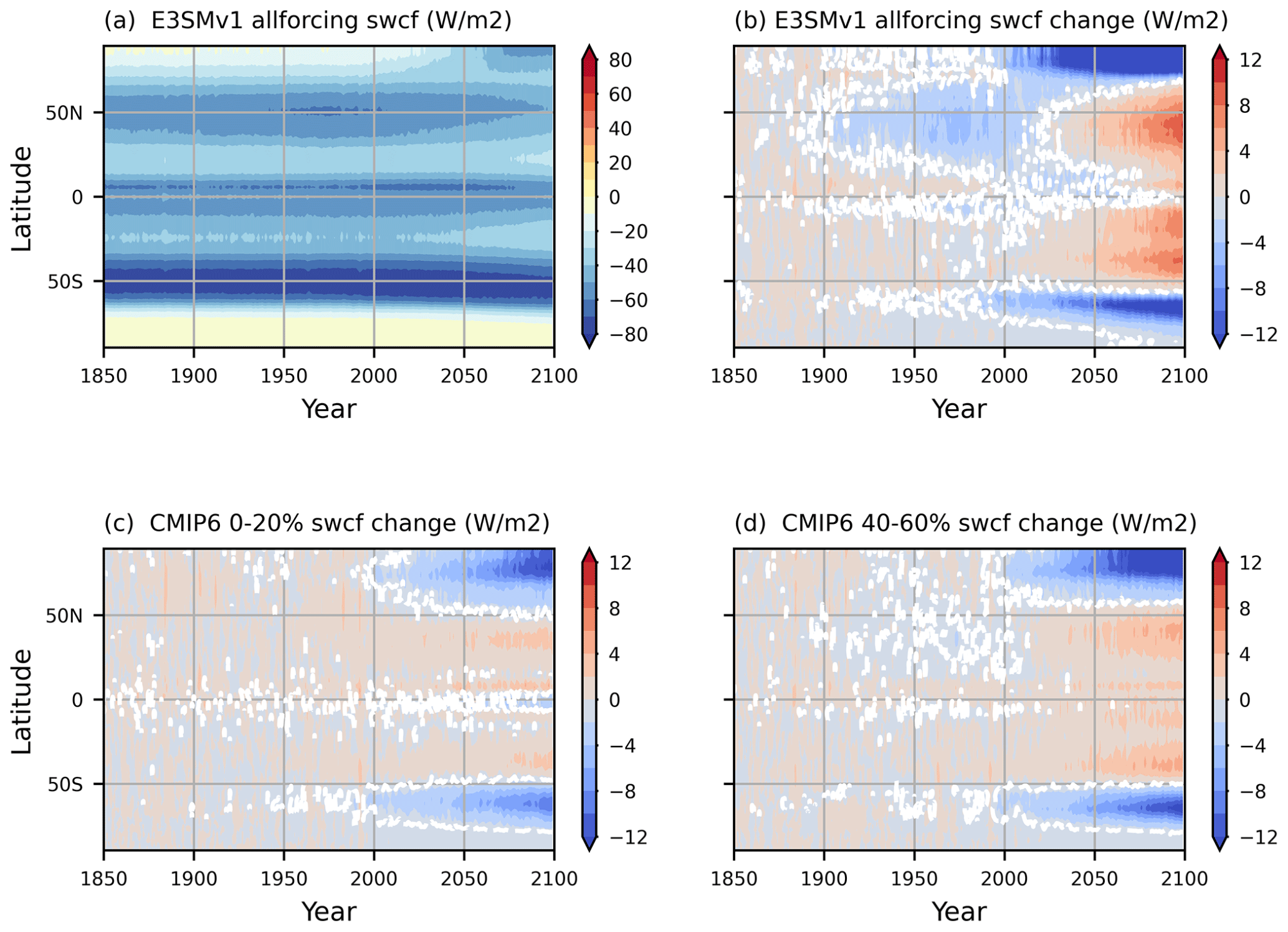
Figure 6Time evolution of zonal mean (a) SWCRE for E3SMv1.0. Time evolution of the local changes in zonal mean SWCRE with respect to 1850–1869 from the historical simulations and SSP5-8.5 future climate simulations (b) E3SMv1.0, (c) CMIP6 models within the 0–20th percentiles, and (d) the 40–60th percentiles.
After the year 2000, Tair in E3SMv1.0 and other CMIP6 models starts increasing, especially over the polar regions. E3SMv1.0 shows a clearly faster warming over the Arctics than CMIP6 models with low and median warming, indicating a stronger polar amplification in E3SMv1.0. The stronger polar amplification tends to be associated with lower sea-ice concentrations, the weaker poleward ocean heat transport at high latitudes, and increases in cloud cover over the polar regions (Holland and Bitz, 2003; Pithan and Mauritsen, 2014; Cohen et al., 2020). Indeed, the negative changes in SWCRE over the polar regions, an indicator of the increased polar cloud amount, in E3SMv1.0 are stronger and are enhanced faster than CMIP6 models with low and median warming after the year 2000 (Fig. 6). However, the regions with a strong negative SWCRE changes in E3SMv1.0 are confined to higher latitudes in both hemispheres. Especially after the year 2050, the region with a strong negative SWCRE change in the Northern Hemisphere retreats to latitudes higher than 60∘ N in E3SMv1.0, while the weakening of the negative SWCRE (i.e., a positive change in SWCRE in Fig. 6) becomes much stronger and broader in low latitudes and midlatitudes compared with the CMIP6 models with low and median warming. Overall, the clouds in E3SMv1.0 show a slightly stronger but more confined negative SW feedback in the high latitudes, while a much stronger and broader positive SW feedback in the low latitudes and midlatitudes relative to CMIP6 models with low and median warming. Compared with CMIP6 models with medium warming, while the E3SMv1.0 simulated negative SWCRE change in the Arctic is stronger than −12 W m−2 after 2050, the positive SWCRE change in both Northern Hemisphere and Southern Hemisphere low latitudes and midlatitudes increases after 2050 and the difference exceeds 8 W m−2 by 2100 (Fig. 6b and d). Meanwhile, the near-surface warming across the low latitudes, midlatitudes, and high latitudes after 2050 (Fig. 5b) indicates that the strong warming in E3SMv1.0 is primarily due to a stronger polar amplification and stronger positive cloud feedbacks from decreasing extratropical low cloud coverage and albedo (Zelinka et al., 2020). Throughout the historical period and the future climate projection period, E3SMv1.0 produces an interhemispheric asymmetric cooling between 1900 and 2000, followed by an interhemispheric asymmetric warming until the end of the 21st century, both of which are closely linked to the cloud responses, especially in the Northern Hemisphere. A recent study (Wang et al., 2021) found that CMIP6 models with a more positive cloud feedback tend to have a stronger cooling effect from aerosol–cloud interactions. The CMIP6 models with a weak aerosol indirect effect and a low cloud feedback are more consistent with the observed warming asymmetry during the mid–late 20th century. We will discuss the impact of the strong aerosol indirect effect in E3SMv1.0 on the future climate projection in Sect. 3.2.1.
3.1.2 Ocean and sea ice
The time evolution of sea surface temperature (SST) anomaly reference to the mean over 1870–1899 (Fig. 7a) in the historical and SSP5-8.5 simulations is consistent with that of Tair in Fig. 1a. The simulated SST anomaly in E3SMv1.0 historical simulations shows relatively weaker warming among the CMIP6 models. It agrees with the Hadley-NOAA/OI merged data product (red Shea et al., 2020) pretty well, except slightly cooler than the data during 1950–1990, mostly occurring in the Northern Hemisphere (Golaz et al., 2019). In the SSP5-8.5 simulations, however, E3SMv1.0 projects a much faster warming than most of other CMIP6 models. By the end of the year 2099, SST in E3SMv1.0 increases by ∼ 5 ∘C compared to the present state, the strongest warming among the CMIP6 models. Note that the CMIP6 models used in Sect. 3.1.1 are slightly different from the CMIP6 models in this section due to the availability of model output varying between the atmospheric variables, ocean, and sea-ice variables.
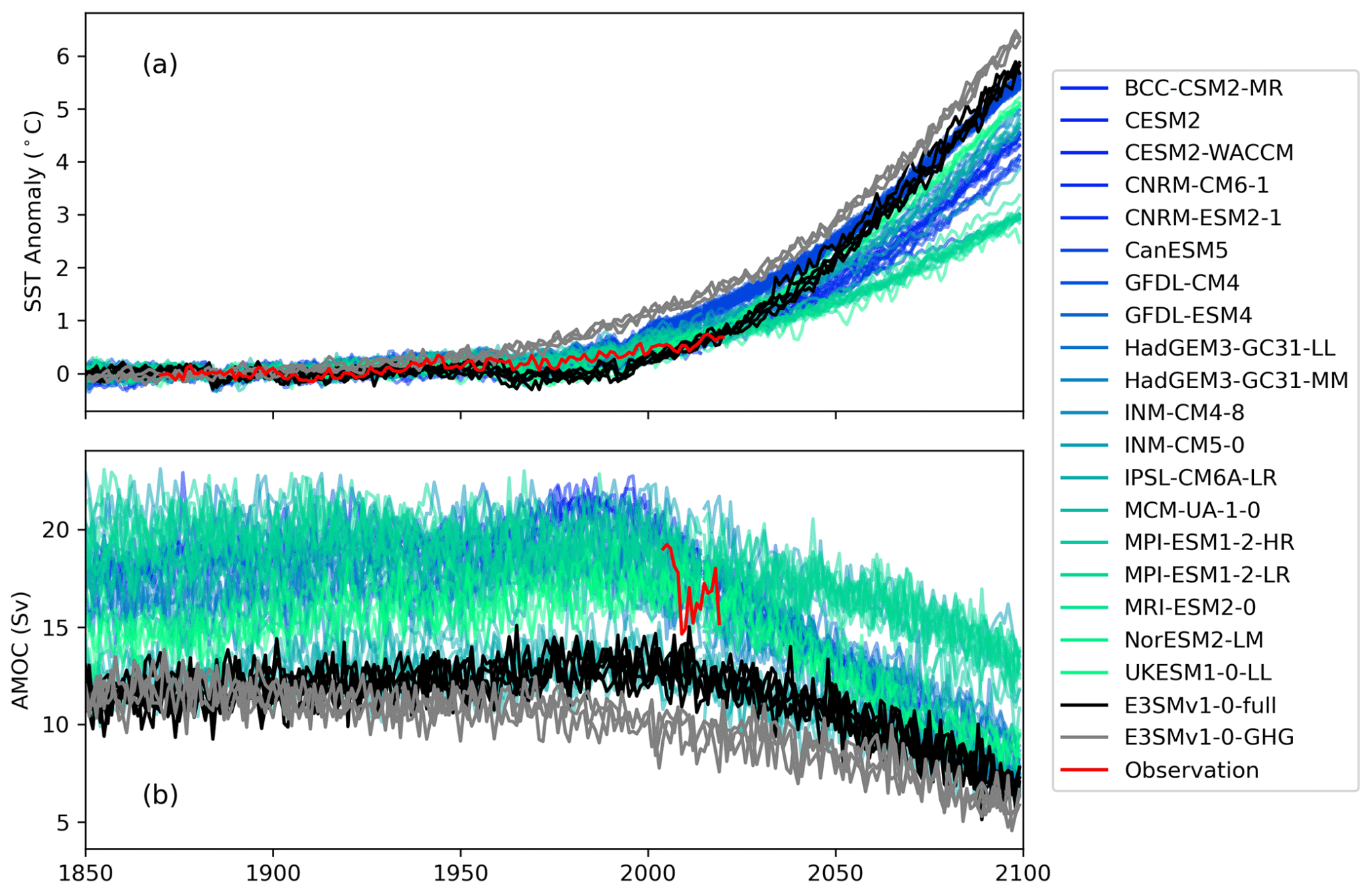
Figure 7Time evolution of (a) annual and global mean SST (∘C) anomaly reference to the mean over 1870–1899 and (b) annual mean AMOC (1 Sv = 106 m3 s−1) in E3SMv1.0 (black), E3SMv1.0 GHG-only (gray), CMIP6 models (blue to green colors), and observations (red). The SST observation is from the Hadley-NOAA/OI merged SST product (Shea et al., 2020). The AMOC is measured by the maximum streamfunction at 26.5∘ N below 500 m depth, consistent with the observation at the RAPID array (Frajka-Williams et al., 2021). Different ensemble members of the same model are denoted using the same color.
Together with the SST anomaly, we plot the simulated annual mean Atlantic meridional overturning circulation (AMOC) in E3SMv1.0 and other CMIP6 models in Fig. 7b, measured by the maximum streamfunction at 26.5∘N below 500 m depth, consistent with the observation at the RAPID array (Frajka-Williams et al., 2021). The mean AMOC simulated in the E3SMv1.0 historical ensemble (∼ 11 Sv) is weaker than the observed mean (16.9 Sv) and the ensemble mean of CMIP6 models (Weijer et al., 2020). It is also at the lower end of the CMIP6 ensemble for the future SSP5-8.5 climate projection. Possible reasons have been discussed in Golaz et al. (2019), including the spurious diapycnal mixing, poor representation of the Nordic overflows, and critical passageways transporting freshwater from the Arctic, as well as excess simulated sea ice in the Labrador Sea in E3SMv1.0.
Interestingly, E3SMv1.0 also exhibits the slowest weakening of AMOC among all the CMIP6 models available in the SSP5-8.5 experiment. This is better seen in Fig. 8, which shows the changes in AMOC and SST between the mean states at the end of the historical and SSP5-8.5 simulations (averaged over 1985–2014 and 2070–2099, respectively). Consistent with Hu et al. (2020), a weaker simulated AMOC is often associated with a weaker change in AMOC in response to the SSP5-8.5 forcing (Fig. 8a), and this often corresponds to a faster warming (Fig. 8c). In addition to the comparison of E3SMv1.0 and CESM2 explored in their study, here we show that this relation also seems to be valid for a group of other CMIP6 models. We note that the simulated mean and change of SST do not seem to show a clear linear relationship as seen in the simulated AMOC, presumably due to the fact that SST is controlled by multiple factors happening at different temporal and spatial scales (e.g., air–sea coupling, ocean mixing). But it is interesting to see a linear relation between the changes in SST and changes in AMOC even within the ensemble of a particular model (e.g., IPSL-CM6A-LR, MPI-ESM1.2-HR, and MPI-ESM1.2-LR in Fig. 8c).
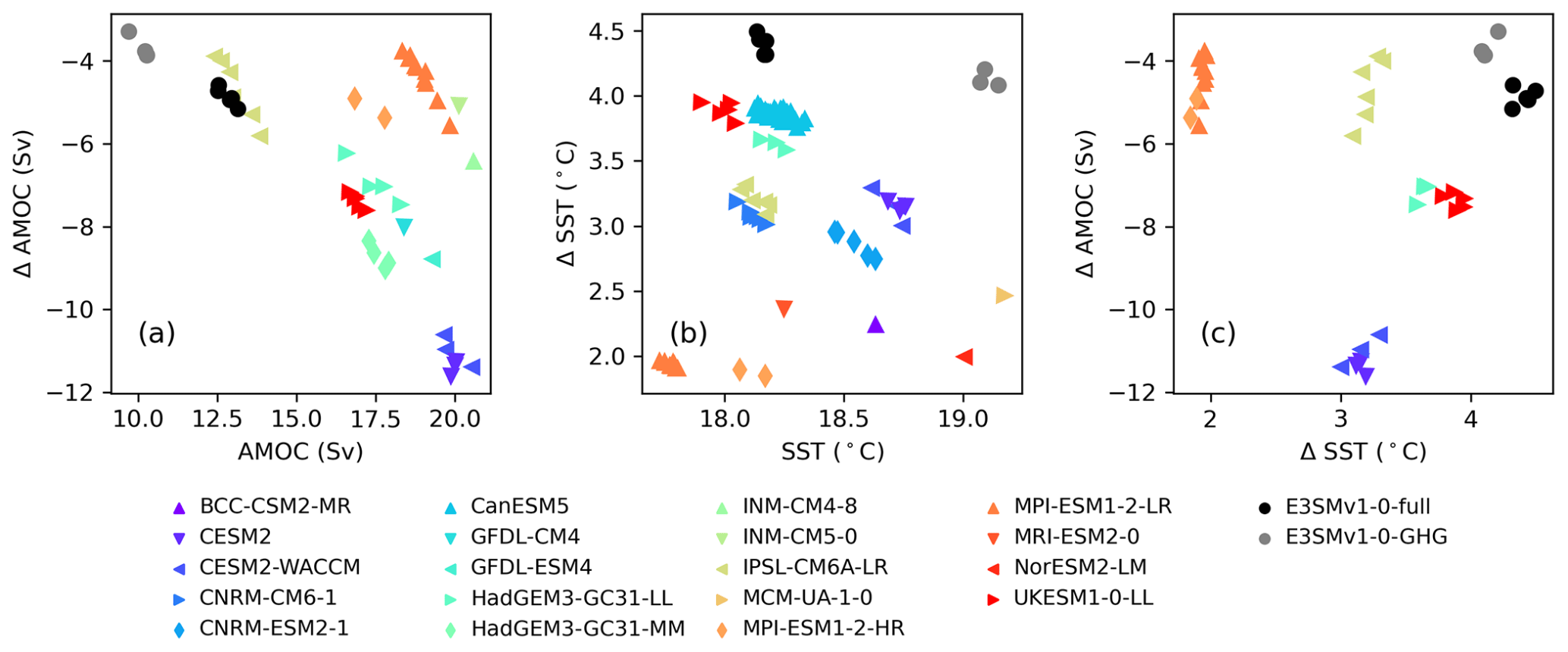
Figure 8Scatter plot showing (a) the change in AMOC versus the reference AMOC, (b) the change in SST versus the reference SST, and (c) the change in AMOC versus the change in SST in the SSP-8.5 experiment. The reference AMOC and SST are the average over 1985–2014 and the changes are measured by the difference between the average over 2070–2099 and the reference.
The ocean has a larger thermal inertia than the atmosphere so there is a delay in the seasons in the ocean as compared to the atmosphere. It is conventional to use January–February–March for boreal winter and July–August–September for boreal summer to describe the seasonal variation of ocean variables. Figure 9a and b show the changes in the ensemble averaged SST in E3SMv1.0 between the period of 2070–2099 and 1985–2014 in the boreal winter (January, February, March) and summer (July, August, September). We see a warming in excess of 2 ∘C almost everywhere in the global ocean, especially in the high latitudes in boreal summer, when the changes in SST can reach over 10 ∘C locally. This is consistent with the strong polar amplification described in Sect. 3.1.1. Correspondingly, there is a strong freshening in the Arctic in both seasons as illustrated by the changes in the sea surface salinity (SSS) in Fig. 10a and b. This is a result of the melting sea ice in the Arctic due to the polar amplification of global warming. The overall decrease in SSS in the North Atlantic and increase in SST in the South Atlantic may be related to the weakening of the AMOC. The mixed layer generally shoals due to an overall warming throughout the global ocean. This is especially true for the winter mixed layer depth (MLD), e.g., the Kuroshio and Gulf Stream extensions in boreal winter and the Southern Ocean in boreal summer in Fig. 11. Figure 12a and b show the ensemble averaged spatial patterns of the simulated AMOC in historical simulations and the changes in SSP5-8.5 simulations. In addition to the latitude and depth of the maximum AMOC, strong weakening also occurs at high latitudes around 50∘ N. This may be linked to the melting of sea ice and weakening of deep water formation in the high-latitude North Atlantic.

Figure 9Panels (a) and (b) show the changes of the ensemble averaged SST (∘C) between the period of 2070–2099 and 1985–2014 in (a) January, February, and March (JFM), and (b) July, August, and September (JAS) in the E3SMv1.0 all-forcing simulations. Panels (c) and (d) show the differences in the SST change between all-forcing simulations and GHG-only simulations. Dots in panels (c) and (d) highlight the regions where such differences are significant as compared to the variations among ensemble members. See the text for more details on how the significance is quantified.
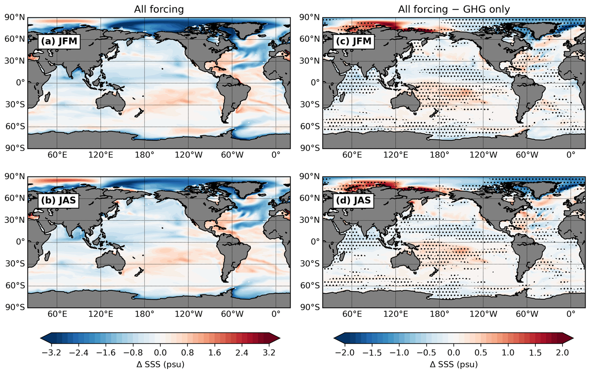
Figure 10Same as Fig. 9 but for the SSS (psu).
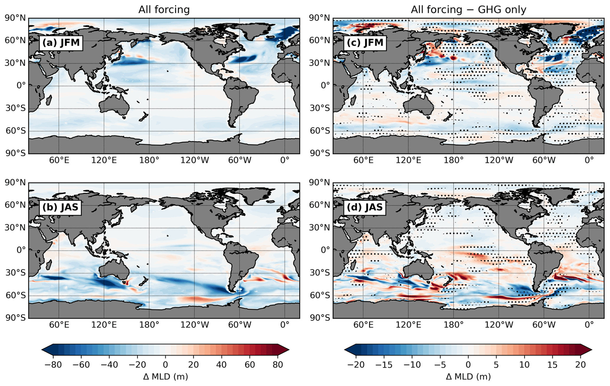
Figure 11Same as Fig. 9 but for the MLD (m) based on a critical density threshold of 0.03 kg m−3.

Figure 12Ensemble averaged spatial patterns of (a, c) the mean and (b, d) changes of AMOC in (a, b) all-forcing simulations and (c, d) GHG-only simulations. The mean is averaged over the period of 1985–2014. The changes shows the difference between the period of 2070–2099 and 1985–2014.
The time series of total sea-ice area in March and September for E3SMv1.0 and CMIP6 models are shown in Fig. 13, together with the observed sea-ice area from the National Snow and Ice Data Center Sea Ice Index version 3 (Fetterer et al., 2017). The simulated sea-ice area in E3SMv1.0 historical simulations agree reasonably well with the observation in September but is significantly larger in the Northern Hemisphere and smaller in the Southern Hemisphere in March. In general, however, the simulated sea-ice area in E3SMv1.0 is within the spread of CMIP6 models in historical simulations. Under the SSP5-8.5 forcing scenario, the projected Northern Hemisphere sea-ice reduction in E3SMv1.0 is faster than most of CMIP6 models with large seasonal variability. While it is comparable with other CMIP6 models in March at the beginning of the SSP5-8.5 simulations (Fig. 13a), the sea ice in September is less than that in most of CMIP6 models and rapidly deceases to zero after the year 2040 (Fig. 13b). The Northern Hemisphere sea ice in March rapidly decreases around 2050 and reduces to near zero after 2080. The Southern Hemisphere (SH) sea-ice reduction is within the wide model spread for both March and September (Fig. 13c and d). Analyses conducted during the development of E3SMv2.0 have shown that an accounting error in the exchange of frazil ice mass between the ocean and the atmosphere largely contributes to this strong reduction.
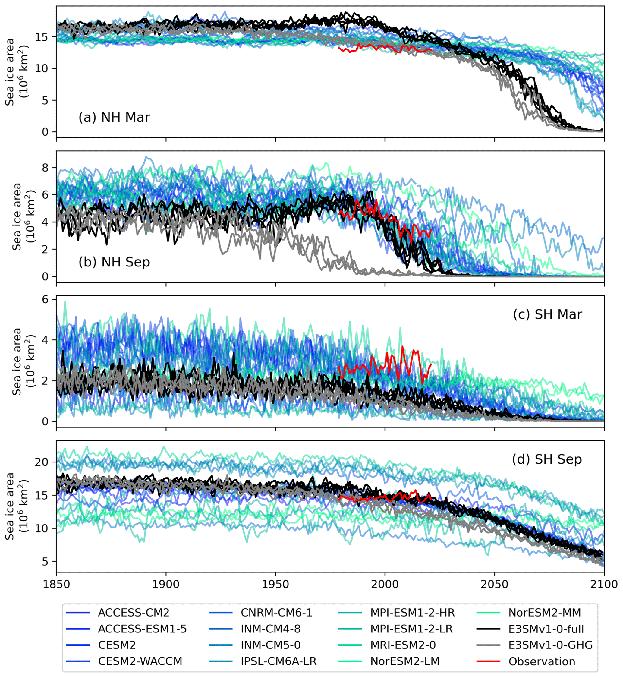
Figure 13Same as Fig. 7 but for (a, b) the Northern Hemisphere and (c, d) Southern Hemisphere sea-ice area (106 km2) in (a, c) March and (b, d) September. The observation is from the National Snow and Ice Data Center Sea Ice Index version 3 (Fetterer et al., 2017). A different set of CMIP6 simulations is used as a reference due to data availability.
3.1.3 Land climatology
Runoff is one of the most representative variables to reflect the land climatology. The spatial patterns of the mean annual runoff for the years 1985–2014 and 2070–2099 (Fig. 14a and b) are generally similar. The patterns are consistent with the DECK simulation results by E3SMv1.0, which had noticeable wet biases over the arid regions such as Australia and the western United States and dry biases over the northern South America (Golaz et al., 2019). The runoff change in the SSP5-8.5 simulations (Fig. 14c) agrees with previous climate change studies (e.g., Nohara et al., 2006) and other CMIP6 model predictions (e.g., Cook et al., 2020) with decreased runoff in the Mediterranean region, southern Africa, southern North America, northern South America, and Australia, and increased runoff in high latitudes of the Northern Hemisphere, central Africa, as well as southern to eastern Asia. Similar to other land surface models, annual runoff predicted by ELMv1 is highly correlated with the precipitation changes (Fig. 3). The Pearson correlation coefficients between the mean annual precipitation and mean annual runoff are 0.9 and 0.89 over the historical period (1985–2014) and future projection period (2070–2099), respectively, suggesting a high similarity in terms of the spatial pattern between the two variables. The time series of annual mean precipitation and runoff anomaly for the entire historical and future projection period (1850–2099) has a correlation coefficient of 0.99, indicating a strong correlation in terms of temporal variation between precipitation and runoff. Given that the spatial distribution and variation of the runoff are highly consistent with those in precipitation for E3SMv1.0, it is fair to presume that the position of E3SMv1.0 simulated global runoff in the CMIP6 ensemble spread is also similar to the global mean precipitation in the ensemble spread (Fig. 1b).
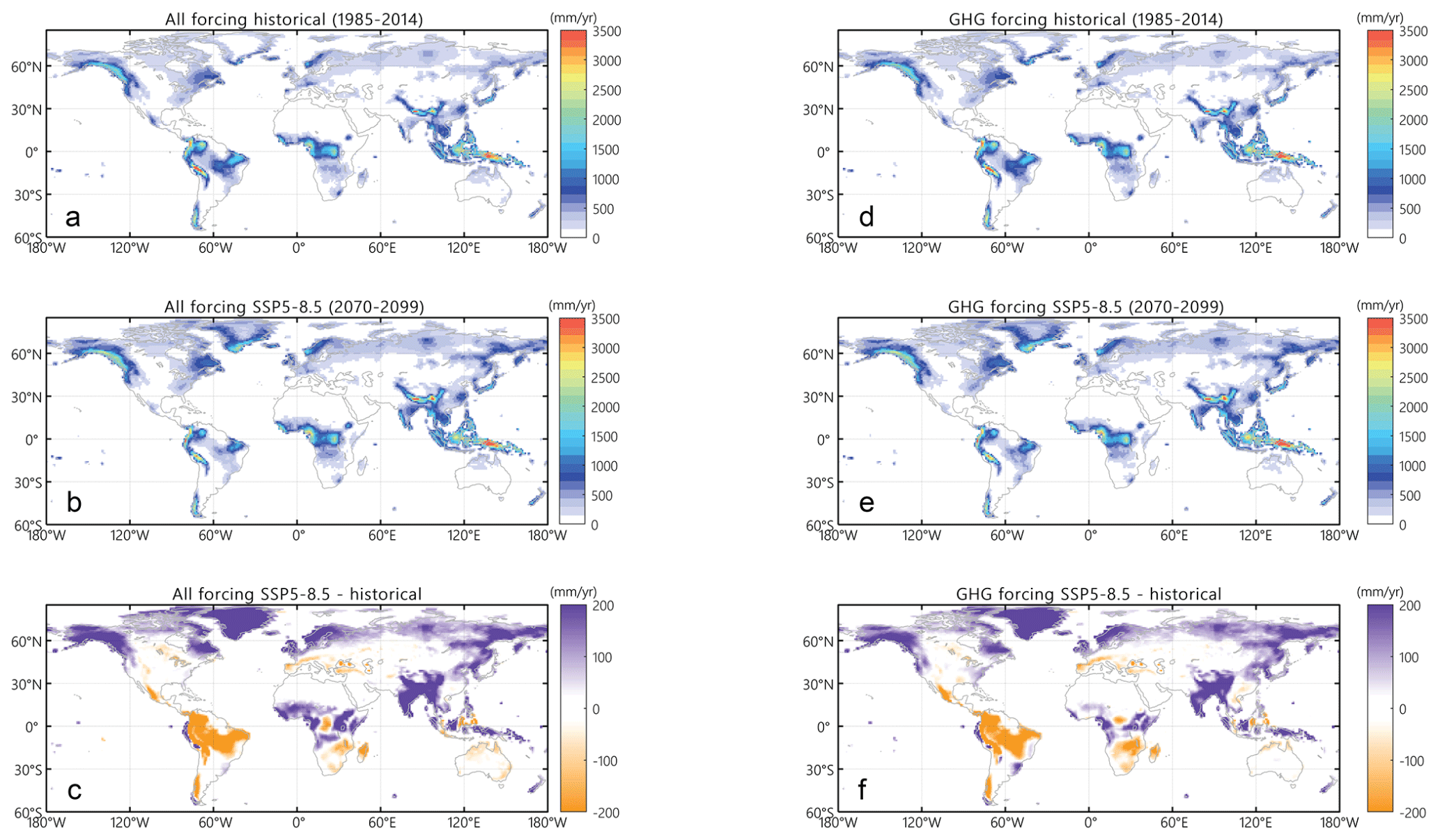
Figure 14(a–c) Annual mean runoff (mm yr−1) from (a) five historical ensemble simulations (1985–2014), (b) five SSP5.85 ensemble simulations (2070–2099), and (c) the change between the time period of 2070–2099 and the period of 1985–2014. Panels (d)–(f) are the same as (a)–(c) except for three ensemble members of the E3SMv1.0 GHG-only experiment.
3.2 GHG-only experiment
As shown in Fig. 1, the climate in the GHG-only experiment warms more rapidly than the all-forcing experiment in the historical simulations and it is warmer than the SSP5-8.5 simulations. Meanwhile, the SST is warmer, the sea-ice amount is less and the AMOC is further weakened in the GHG-only experiment compared to the SSP5-8.5 experiment (Figs. 7 and 13). Previous modeling and observational studies have controversial findings on the contribution of GHG forcing vs. other forcings to the historical climate change and the future climate projection. While studies indicate that human-induced GHG forcing has dominated observed global warming since the mid-20th century (Jones et al., 2013), some studies found that both GHG and aerosol changes contribute to warming during the 21st century (Gillett et al., 2012) and aerosol forcing is found to determine intermodel variations in the historical surface temperature for CMIP5 models (Rotstayn et al., 2015). Beyond these general features of the changes in surface temperatures, AMOC, and sea ice, the following subsections focus on the differences between the historical and SSP5-8.5 experiments (i.e., the all-forcing simulations) and the corresponding GHG-only experiments, which will shed light on the contribution of the GHG forcing to the E3SMv1.0 simulated climate change in the history and future projection relative to the other forcings.
3.2.1 Atmospheric responses
In the absence of all other external forcing, the global mean Tair increases monotonically in the GHG-only historical experiment (Fig. 1). Unlike in the all-forcing historical experiment, the Tair and SWCRE changes show no signal of cooling and enhanced cooling effect in the Northern Hemisphere (Fig. 15a and b) over the regions with a clearly higher aerosol load in the all-forcing historical experiment, a significant portion of which is sulfate aerosol (Fig. 15e and f). The net cloud radiative effect (CRE) shows an extra strong cooling effect up to −5 W m−2 over the previously mentioned region and period in the all-forcing historical experiment (Fig. 15d). This further confirms that the overly strong ERFaero, including the strong aerosol–cloud interactions, causes the prolonged cooling between 1960 and 2000 and the delayed warming after 2000 in the E3SMv1.0 historical experiment. Near the end of the historical simulations, Tair is warmer almost everywhere in the GHG-only historical experiment, especially over the Arctic (Fig. 2c vs. d, Fig. 5b vs. Fig. 15a).
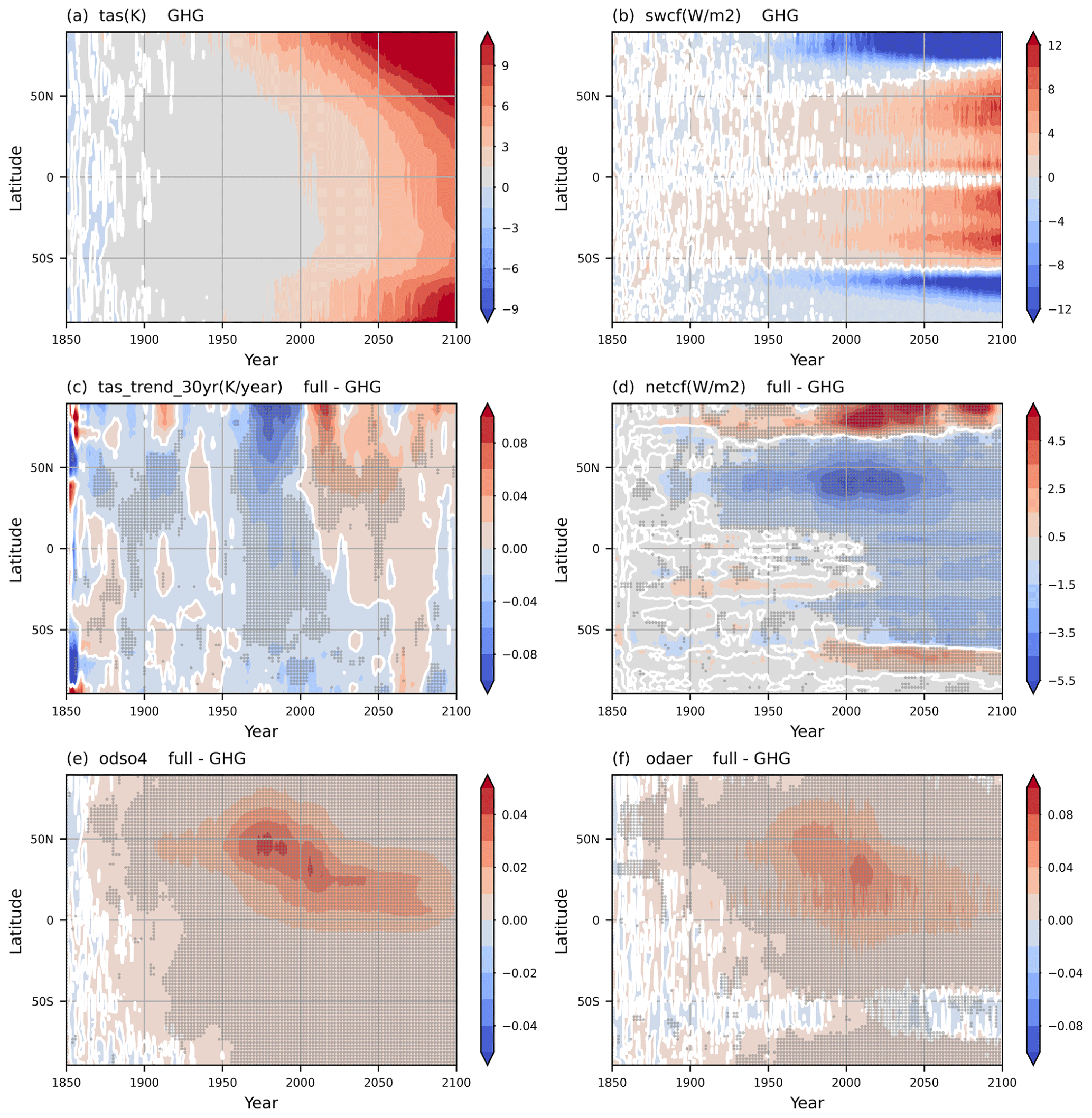
Figure 15The time evolution of the zonal mean local (a) Tair change (K), (b) SW cloud radiative forcing (W m−2) in E3SMv1.0 GHG-only simulations, and the simulated differences in (c) Tair trend (K yr−1), (d) net cloud radiative forcing (W m−2), (e) sulfate aerosol optical depth at 550 nm, and (f) total aerosol optical depth at 550 nm between E3SMv1.0 all-forcing simulations and GHG-only simulations. Stippled regions in panels (a)–(c) indicate where the difference reaches the 95 % confidence level based on a two-tailed Student's t test.
In the SSP5-8.5 GHG-only experiment, although Tair increases with a spatial pattern similar to the SSP5-8.5 all-forcing experiment, the warming slows down after 2000 compared to the SSP5-8.5 all-forcing experiment based on the zonal mean Tair trend, suggesting that the decline of aerosol load in the future climate projection period leads to a transient faster warming in the 21st century (Fig. 15e and f). Also, the polar amplification is weaker in the GHG-only experiment (Fig. 15c). Note that the delayed warming between 1970 and 2000 in the all-forcing experiment relative to the GHG-only experiment is statistically significant based on a two-sided t test, while the faster warming after 2000 is not statistically significant in many regions. The global distribution of the warming between 2070–2099 and 1985–2014 from the GHG-only experiment also shows weaker warming in the Northern Hemisphere than the all-forcing experiment with a poleward increased difference (Fig. 2e–f). The difference in the net CRE between the all-forcing experiment and the GHG-only experiment during the future climate project period (Fig. 15d) may contribute to the weaker polar amplification in the GHG-only experiment. Previous studies detected rapid near-term warming through the 21st century driven by decrease in aerosols in CMIP5 models (e.g., Chalmers et al., 2012; Levy II et al., 2013), whereas aerosol emission reduction caused gradual warming in other CMIP5 studies (e.g., Gillett and Salzen, 2013). Further simulations and analyses will be needed to fully understand the mechanism underlining the accelerated warming in the Northern Hemisphere, which is beyond the GHG-induced warming.
During the historical period, the global precipitation in the GHG-only simulations is larger than that in the all-forcing simulations by 0.13 mm d−1 (∼ 4 %) at the end of the historical period (Fig. 1b). The global maps (Fig. 3c and d) indicate that the GHG-only experiment is overall similar to the all-forcing experiment at the end of the historical period with changes resembling the SSP5-8.5 experiment except for the smaller magnitude, i.e., slightly increased precipitation in the tropics and the midlatitude oceans. The changes in precipitation rate between the future climate projection and the historical period from the all-forcing experiment and GHG-only experiment (Fig. 3e and f) suggest that the magnitude of the precipitation change is larger in the all-forcing experiment especially for the drying regions, e.g., the central and eastern south Pacific, the south Indian Ocean, Australia, and the Amazon region. Meanwhile, the changes over regions with increased precipitation in the future climate projection are generally larger in the all-forcing experiment than that in the GHG-only experiment, e.g., the northern Indian Ocean, the Indian peninsula, and the Tibetan Plateau, midlatitude Eurasia, and the coastal regions of the northern Pacific. One exception is that the drying signal along the tropical eastern Pacific to Central America is stronger in the GHG-only experiment.
3.2.2 Ocean and sea-ice responses
Panels (c) and (d) in Figs. 9–10 show the differences of the SSP5-8.5 projected changes in SST, SSS, and MLD between the all-forcing experiment and the GHG-only experiment. A two-sided t test with the null hypothesis that the GHG-only experiment and all-forcing experiment give identical ensemble mean was conducted. Dots in the maps highlight regions where the p value of the t test is smaller than 5 %, and therefore the difference is significant as compared to the variability among ensemble members.
The spatial distribution of the SSP5-8.5 projected warming, especially the polar amplification in boreal summer (Fig. 9b), is mostly similar between the all-forcing experiment and GHG-only experiment (not shown), with a significantly stronger magnitude in the all-forcing experiment (see the similar spatial patterns between panels c and a, and between d and b). This suggests that while GHG emissions dominate the changes in oceanic mean SST, other forcings may also be important in amplifying the changes. Similar remarks could also be made for the simulated SSS (Fig. 10), though the difference of the simulated SSS between all-forcing and GHG-only experiments are more complicated. The changes in SSS are likely driven by atmospheric forcing, which is indeed evident in the bottom panel of Fig. 3 that the projected reduction of precipitation in the all-forcing experiment is stronger than that in the GHG-only experiment over this region. The difference in the simulated MLD (Fig. 11) between all-forcing and GHG-only experiments is less obvious, especially in regions of strong currents (e.g., the Kuroshio and Gulf Stream extensions and the Southern Ocean) where the variability among ensemble members is large. We also note that the strength of the AMOC is slightly weaker in the GHG-only experiment during most of the period (Figs. 7 and 12). This could be due to the warmer Tair (Fig. 1), which would decrease North Atlantic surface density, thus, reducing deep convection and AMOC. The SSP5-8.5 all-forcing and GHG-only experiments converge toward the end of the simulations. Given that the AMOC is so weak in both experiments, this is likely nearing an “off” state.
The sea-ice extent for the SSP5-8.5 all-forcing experiment and the SSP5-8.5 GHG-only experiment is shown in the black and gray lines respectively in Fig. 13. Overall, the trends are similar, which is not surprising given the strong warming in both experiments. However, we do note that the Northern Hemisphere sea-ice extent in September in the GHG-only experiment decreases rapidly since 1950 and drops to nearly zero around 1990, likely a result of a much warmer state in the GHG-only experiment. The Northern Hemisphere sea-ice extent in March in the GHG-only experiment is also lower than the all-forcing experiment since around 1950, but decreases at a similar rate as the all-forcing simulation between around 2010 and 2050. It decreases rapidly starting from approximately 2050, whereas the sea-ice extent in the all-forcing experiment remains larger for another decade before dropping rapidly. Note that the warming SST in the high-latitude North Atlantic in boreal winter is actually smaller in the GHG-only experiment than in the all-forcing experiment (Fig. 9c). Further, the difference in the net CRE between the all-forcing experiment and the GHG-only experiment (Fig. 15d) over the polar regions suggests more warming from cloud radiative effect for the all-forcing experiment, which is counter to what is observed in Fig. 13. Therefore, the earlier decrease in Northern Hemisphere sea-ice extent in March in the GHG-only experiment may also be driven by the warmer mean climate state in the GHG-only experiments (e.g., Figs. 1 and 7). The Southern Hemisphere sea-ice extent in both March and September is similar between the all-forcing experiment and the GHG-only experiment and only slightly smaller in the latter due to the warmer mean climate state.
3.2.3 Land responses
The land responses were first examined by comparing the runoff distributions driven by all forcing and GHG-only forcing (Fig. 14). No obvious differences can be identified between the runoff during either historical or future period. However, a noticeable deviation can be seen in the historical to future changes (i.e., between Fig. 14c and f). Specifically, in southern North America, southern Africa, and eastern Asia, GHG-only forcing leads to a greater decline in future runoff than all forcing condition, while in central Africa, the GHG-only forcing tends to have less runoff increase in the future than the all forcing condition. To further examine the time evolution of runoff responses in the SSP5-8.5 all-forcing experiment and the SSP5-8.5 GHG-only experiment, we applied the two-sample Kolmogorov–Smirnov (K-S) test on the annual mean runoff at grid-cell level. The two-sample K-S test has been widely applied in climate studies (e.g., Wang et al., 2008; Zhou et al., 2018; Gaetani et al., 2020) to examine whether two data samples are from a same distribution by comparing their empirical cumulative distribution functions (eCDFs). The null hypothesis (H0) is that the values of two data sets are from the same continuous distribution, which can be rejected at a significant level (α) if
where (m,n) are the sample sizes of the two samples; (Dm,n) is the distance between the eCDFs of the two samples; (i(α)) is the inverse of the Kolmogorov distribution at (α). The smaller (Dm,n), the more similarity between the to eCDFs. In this study, the K-S test was conducted for mean annual runoff at every land grid cell between the SSP5-8.5 all-forcing experiment and GHG-only experiment with (α=0.01). Similar to previous sections for other climate components, we selected two 30-year periods to represent historical (1985–2014) and future (2070–2099) conditions. In the following context we will use letter R to indicate H0 was rejected, meaning the two samples (i.e., runoff from the all-forcing experiment and GHG-only experiment) are from different distributions; and letter F to indicate H0 was fail to reject, meaning the two samples are from the same distribution. Two representative pixels were picked to further demonstrate the changes in runoff time series as well as the eCDFs for the two different directions of changing (Fig. A3 for F to R, and Fig. A4 for R to F).
The global distribution of the K-S test results for the historical period (Fig. 16a) were F in most areas but R in Greenland, Australia, central and northwest of North America, and eastern Asia. For the future climate projection period (Fig. 16b), the F area was generally expanded, indicating the difference in local runoff enlarges in the future climate projection experiments. Note that, some areas turn from R to F, such as Greenland, Australia, and Alaska, meaning that the time evolution of the local runoff from the all-forcing experiment and GHG-only experiment become closer to each other during the future climate projection period. The difference in local runoff during both time periods will contribute to the difference in the projected runoff change between the SSP5-8.5 all-forcing experiment and the GHG-only experiment (Fig. 14c and f). Therefore, the regions with F in either period (Fig. 16a and b) tend to have notable differences in the projected runoff changes shown between Fig. 14c and f.
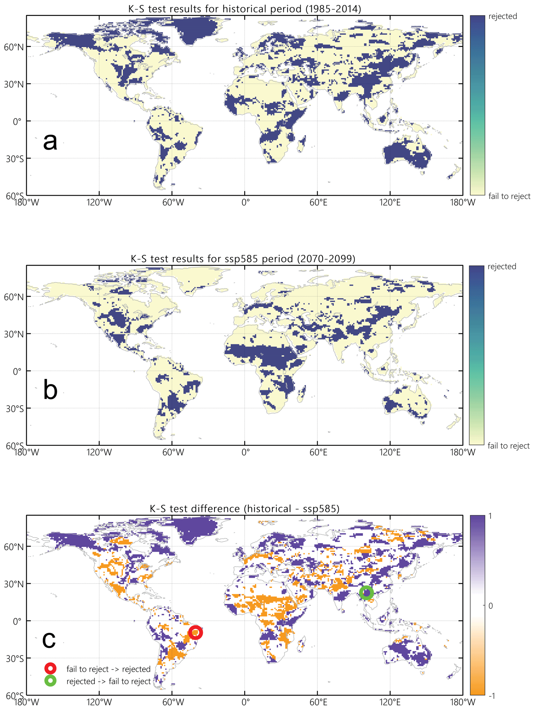
Figure 16Two-sample K-S test results for mean annual runoff over a (a) 30-year historical period (1985–2014), (b) 30-year ssp585 period (2070–2099), with “rejected” indicating the two samples are not from the same distribution and “fail to reject” indicating the two samples are from the same distribution. The time series and eCDF for two pixels marked with circles in panel (c) are shown in Figs. A3 and A4.
The difference between the K-S test results (Fig. 16c) clearly shows the regions with a switch in runoff changes from the historical period to the future climate projection period, where K-S test results changed from R to F (i.e., purple regions in Fig. 16c). We also noticed that the K-S test results in some areas, such as central Africa, changed from F to R which is opposite to the general trend. Overall, about 14 % of the global area changed the results from F to R (orange color) and 26 % area changed from R to F (purple color) nearly doubled. This suggests that the runoff distributions from the SSP5-8.5 all-forcing experiment and GHG-only experiment tend to be more similar during the future period than during the historical period, implying that the GHG emission plays a dominant role among all forcings in terms of runoff for the future climate projection period. Instead of investigating changes in annual mean (Fig. 14c and f), K-S tests focus on the distributional changes and thus provide additional information associated with systematic alteration in the time series. One limitation of our current annual scale runoff analysis is that it did not fully address the snow dynamic changes, which are mostly associated with seasonal shifts in runoff due to changes in snow accumulation and melting processes, as well as snow versus rain partitioning of the precipitation (Cook et al., 2020; Knutti and Sedláček, 2013). Therefore, to better understand the contribution of forcings on the runoff changes, seasonal runoff analysis will be needed in the future studies.
In this paper, we describe the experimental setup and general features of the coupled historical and future projection simulations that E3SMv1.0 contributes to ScenarioMIP of CMIP6. We conducted two sets of coupled E3SMv1.0 experiments in the highest-emission SSP5-8.5 scenario: (1) the all-forcing experiment designed in the ScenarioMIP project, and (2) the SSP5-8.5 GHG-only experiment inspired by the DAMIP project. Both experiments include the historical simulations (years 1850–2014) and the future projection simulations (years 2015–2099). Five ensemble members were generated for the SSP5-8.5 all-forcing experiments, while three ensemble members were conducted for the GHG-only experiments. Analyzing the ensemble means, we describe the global and regional responses of atmosphere, ocean, sea ice, and land runoff during the whole period. The currently available ScenarioMIP simulations from other CMIP6 models serve as a reference to characterize the E3SMv1.0 simulations. Furthermore, we estimate regional responses of key climate components in the GHG-only simulations in comparison with these in the all-forcing experiment. The relative impacts of GHG forcing vs. other forcing on the future projections of the different climate components are analyzed and reveal the following features about the future climate projection by E3SMv1.0:
-
E3SMv1.0 is one of the CMIP6 models with the largest surface warming by the end of the 21st century under the SP5-8.5 scenario, which is consistent with the overly strong TCR and ECS of E3SMv1.0. The global surface precipitation rate increases along with the surface warming. The regional patterns of the projected precipitation change by E3SMv1.0 are consistent with the ensemble average pattern from the ScenarioMIP participant models for the SSP5-8.5 scenario. The regions with significantly increased precipitation include ITCZ, North America, and most of the Eurasian continent. The major drying regions include the Mediterranean region, Central America, the Amazon region, southern Africa, and western Australia, regions where dry biases exist in the historical simulations (Golaz et al., 2019). The spatial pattern of the change in land runoff is highly correlated with the precipitation changes.
-
The global SST increase is similar to Tair with a much faster warming than most of other CMIP6 models. Meanwhile, the oceanic mixed layer generally shoals due to the overall warming throughout the global ocean. The annual mean AMOC is at the lower end of the CMIP6 ensemble for the future climate projection. The change in AMOC is weaker in response to the SSP5-8.5 forcing, which likely contributes to the faster warming in E3SMv1.0. The sea-ice reduction, especially over the Northern Hemisphere, is faster than that of most of the CMIP6 models with large seasonal variability.
-
There is a strong signal of polar amplification in E3SMv1.0 shown as a strong Tair and SST warming in the Arctic. It is associated with increased clouds, a weaker AMOC, reduced SSS, lower sea-ice concentration, and faster sea-ice melting in the Arctic.
-
The time evolution of the zonal mean Tair shows that E3SMv1.0 has a strong cooling in the Northern Hemisphere midlatitudes between the years 1900 and 2000, which is consistent with the peak aerosol optical depth, supporting the hypothesis of an overly strong aerosol indirect effect.
-
In the SSP5-8.5 GHG-only experiment, the global mean Tair is higher than the SSP5-8.5 all-forcing experiment in both historical and future projection periods. The accelerated warming, however, shown in the SSP5-8.5 all-forcing experiment exceeds the GHG-induced warming in the first half of the 21st century. The accelerated warming is likely linked to the unmasking of the aerosol effects from the decline of the aerosol loading in the future projection period.
-
Comparing the SSP5-8.5 experiment with the GHG-only experiment suggests that the GHG forcing dominates the control of the oceanic climate change. In contrast, land runoff analyses found that the runoff change between the SSP5-8.5 all-forcing experiment and GHG-only experiment is larger over certain regions, e.g., southern North America, southern Africa, central Africa, and eastern Asia especially during the historical period. But the runoff distributions from the all-forcing experiment and the GHG-only experiment tend to become more similar during the future period as the impact of GHG forcing grows and becomes dominant.
As discussed in Sect. 3, this paper mainly describes the experiments and present the most notable features revealed in these experiments. Further model sensitivity tests and in-depth model diagnostics combined with observational references will be required to fully understand the mechanisms causing these general features documented in this study. We are also focusing our analysis on the changes in the mean climate state. While we acknowledge the importance of assessing the possible changes in climate variability (e.g., El Niño–Southern Oscillation; ENSO) in these simulations, a robust detection of changes in climate variability may require a significantly larger ensemble of simulations, which is beyond the scope of this study.
Table A1 lists the CMIP6 models, of which the historical experiment and the SSP5-8.5 all-forcing experiment were included in this study. All those model data have been released the Earth System Grid Federation (ESGF). The DOIs for the data and the reference for the model are listed in the table as well.
Figures A3 and A4 demonstrate how the two-sample K-S test determines the changing directions of the runoff change based on the time series of runoff over a grid point. Figure A3 shows that the runoff change switches from the same distribution during 1985–2014 to the different distribution during 2070–2099 at 9.5∘ S, 40.5∘ W (red circle in Fig. 16c). Figure A4 shows that the runoff change switches from the different distribution during 1985–2014 to the same distribution during 2070–2099 at 22.5∘ N, 100.5∘ E (green circle in Fig. 16c).

Figure A1DJF mean precipitation rate (mm d−1) from (a) five SSP5.85 ensemble simulations (2070–2099), (c) five historical ensemble simulations (1985–2014), and (e) the change between the time period of 2070–2099 and the period of 1985–2014. DJF mean precipitation rate (mm d−1) from (b) three SSP5.85-GHG ensemble simulations (2070–2099), (d) three historical-GHG ensemble simulations (1985–2014), and (f) the change between the time period of 2070–2099 and the period of 1985–2014.
Table A1The list of the CMIP6 models from which the historical experiments and ScenarioMIP experiments are adopted in this study through the Earth System Grid Federation (ESGF).
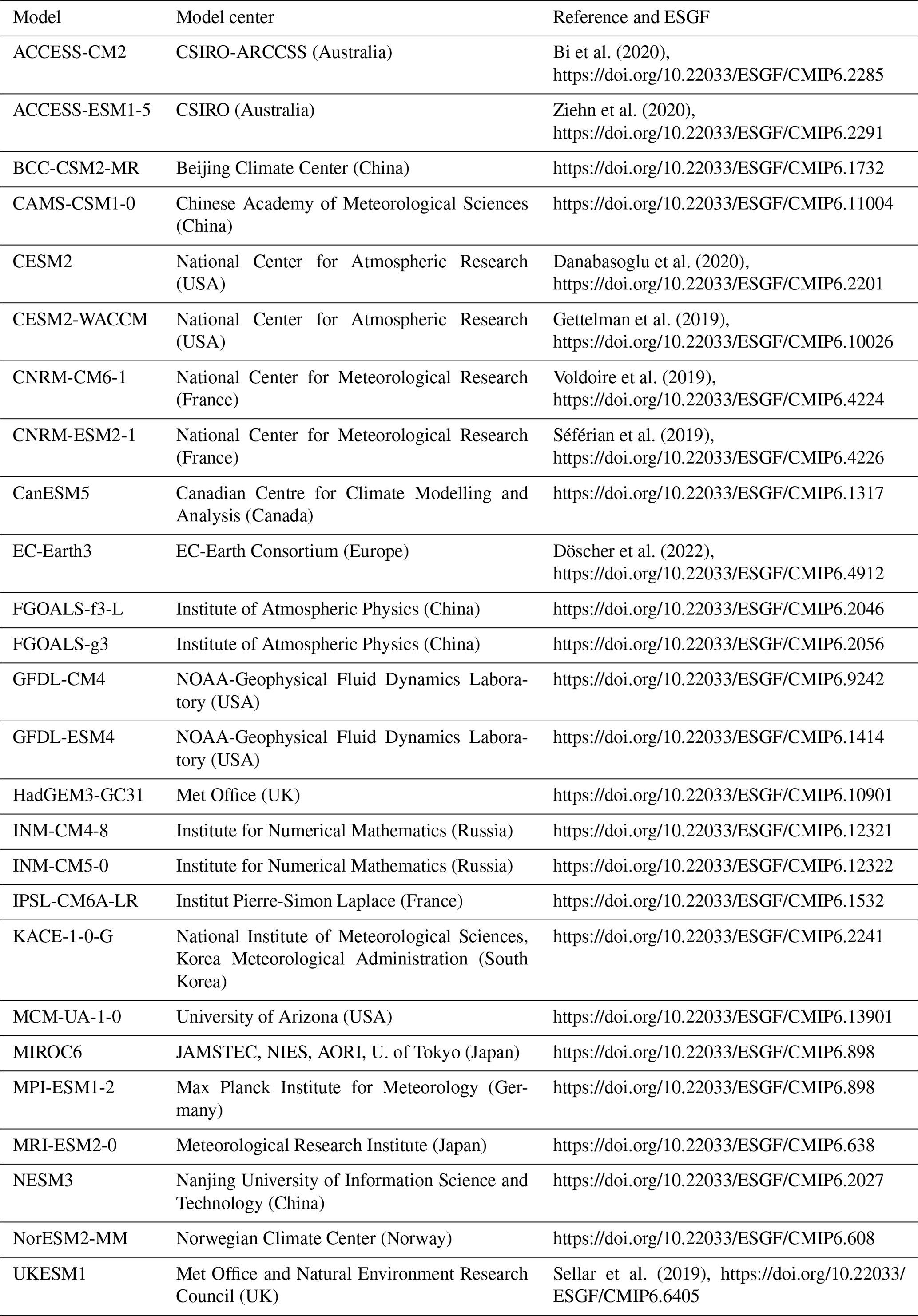
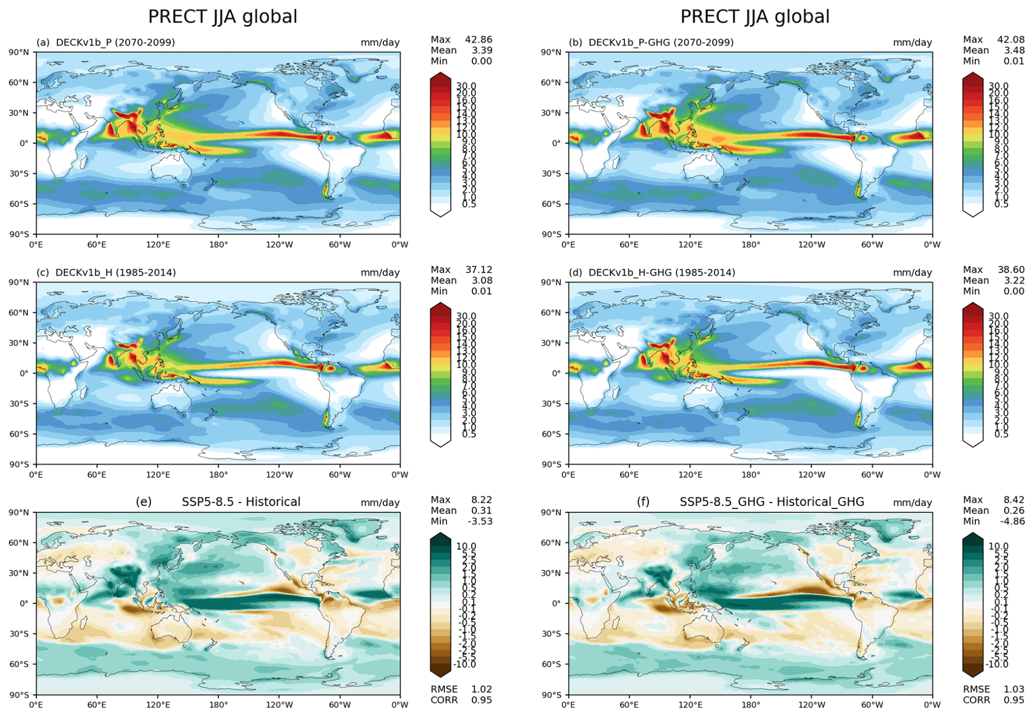
Figure A2JJA mean precipitation rate (mm d−1) from (a) five SSP5.85 ensemble simulations (2070–2099), (c) five historical ensemble simulations (1985–2014), and (e) the change between the time period of 2070–2099 and the period of 1985–2014. JJA mean precipitation rate (mm d−1) from (b) three SSP5.85-GHG ensemble simulations (2070–2099), (d) three historical-GHG ensemble simulations (1985–2014), and (f) the change between the time period of 2070–2099 and the period of 1985–2014.
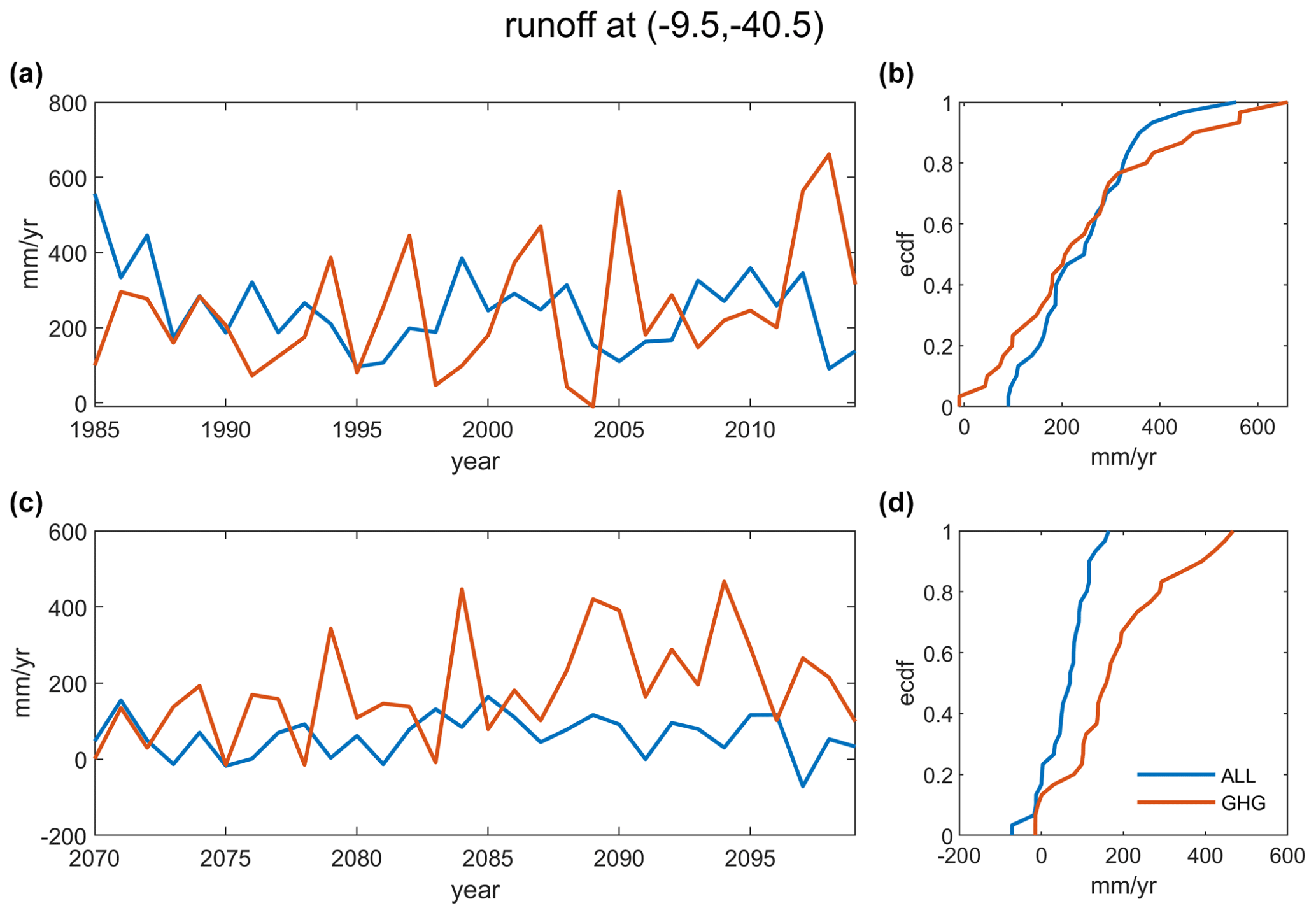
Figure A3The 30-year mean annual runoff time series and eCDF from all forcing and GHG-only forcing simulations for historical period (a, b), and SSP5-8.5 period (c, d) at (9.5∘ S, 40.5∘ W), where the K-S test failed to reject (F) in the historical period and rejected (R) in the SSP5-8.5 period.
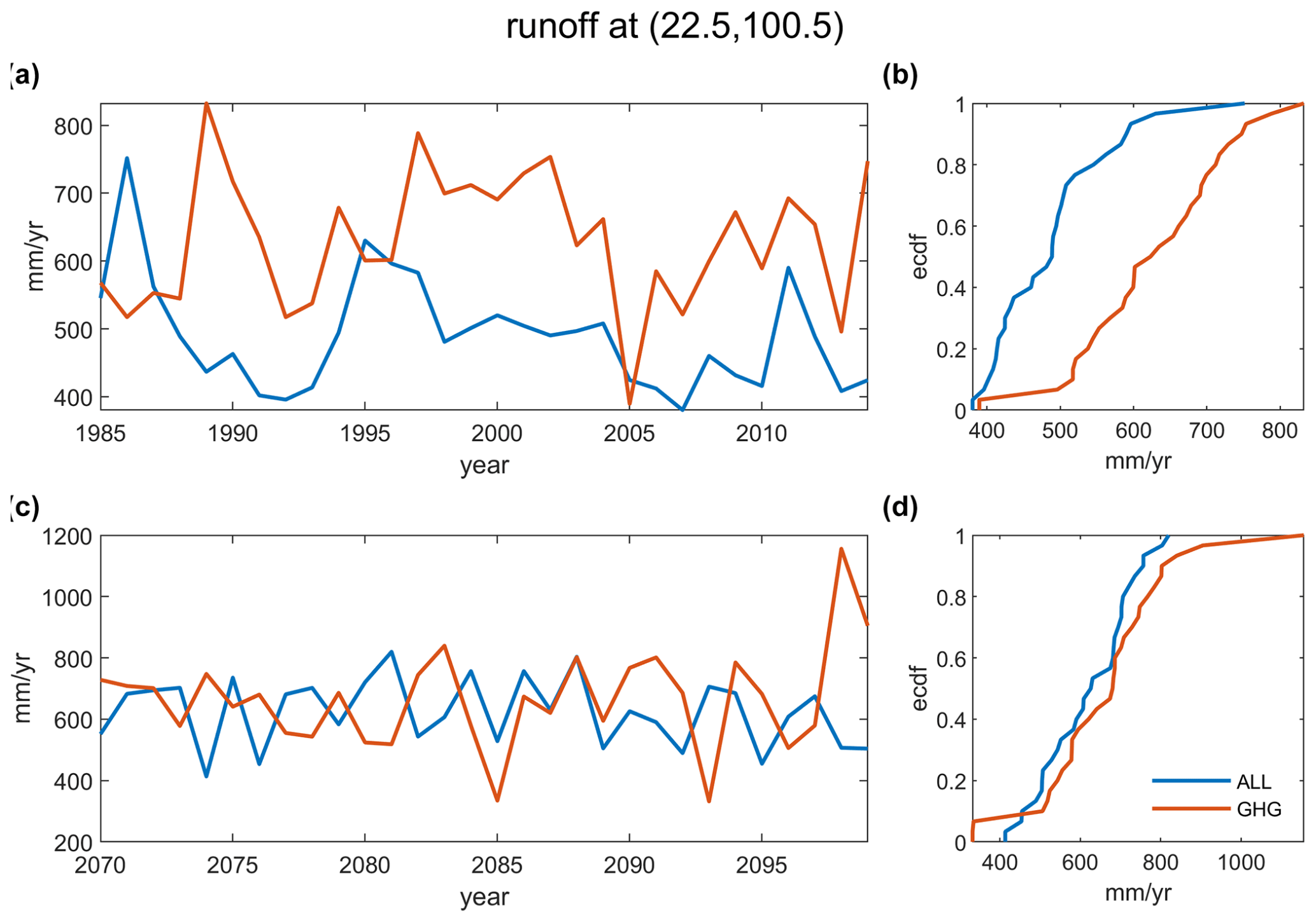
Figure A4The 30-year mean annual runoff time series and eCDF from all forcing and GHG-only forcing simulations for historical period (a, b), and SSP5-8.5 period (c, d) at (22.5∘ N, 100.5∘ E), where the K-S test was rejected (R) in the historical period and failed to reject (F) in the SSP5-8.5 period.
The E3SMv1.0 model code was released at https://doi.org/10.11578/E3SM/dc.20180418.36 (E3SM Project, DOE, 2018).
The E3SMv1.0 historical simulations and future climate simulations data can be accessed on the ESGF platform https://doi.org/10.22033/ESGF/CMIP6.4497 (Bader et al., 2019), https://esgf-node.llnl.gov/search/e3sm/?model_version=1_0&experiment=hist-GHG (last access: 12 May 2022), https://esgf-node.llnl.gov/search/e3sm/?model_version=1_0&experiment=ssp585 (last access: 12 May 2022), https://esgf-node.llnl.gov/search/e3sm/?model_version=1_0&experiment=ssp585-GHG (last access: 12 May 2022).
The run scripts used to set up simulations in this study are available online (https://doi.org/10.5281/zenodo.5498235; Zheng et al., 2021).
XZ coordinated the writing of this article. JCG and QT coordinated, conducted, and archived the simulations for this study. XZ and JCG analyzed and documented the atmospheric results. QL analyzed the ocean and sea-ice results from E3SMv1.0 and other CMIP6 models. QL and LPVR wrote the sections on the ocean and sea ice. TZ analyzed the land runoff from these E3SMv1.0 simulations and wrote the related sections. HW was responsible for producing aerosol emissions input data set based on the original input4MIPS data for the SSP5-8.5 all-forcing experiment. PCS was responsible for producing GHGs and other forcing data sets. All co-authors gave feedback on the manuscript.
The contact author has declared that neither they nor their co-authors have any competing interests.
Publisher's note: Copernicus Publications remains neutral with regard to jurisdictional claims in published maps and institutional affiliations.
This research was supported by E3SM project funded by the Office of Biological and Environmental Research in the US Department of Energy's Office of Science. This research used resources of the National Energy Research Scientific Computing Center (NERSC), a US Department of Energy Office of Science User Facility located at Lawrence Berkeley National Laboratory, operated under contract no. DE-AC02-05CH11231. We thank two anonymous reviewers for their insightful and constructive comments. Figures 2, 3, 4, A1, and A2 are generated by E3SM Diags (see https://e3sm.org/resources/tools/diagnostic-tools/e3sm-diagnostics, last access: 12 May 2022). Xue Zheng, Jean-Christophe Golaz, Qi Tang and Philip Cameron-Smith were supported under the auspices of the US Department of Energy by LLNL under contract no. DE-AC52-07NA27344.LLNL-JRNL-826361. The Pacific Northwest National Laboratory (PNNL) is operated for DOE by the Battelle Memorial Institute under contract no. DE-AC05-76RLO1830.
This research has been supported by the Office of Science (E3SM project).
This paper was edited by Olivier Marti and reviewed by two anonymous referees.
Adler, R. F., Sapiano, M. R. P., Huffman, G. J., Wang, J.-J., Gu, G., Bolvin, D., Chiu, L., Schneider, U., Becker, A., Nelkin, E., Xie, P., Ferraro, R., and Shin, D.-B.: The Global Precipitation Climatology Project (GPCP) Monthly Analysis (New Version 2.3) and a Review of 2017 Global Precipitation, Atmosphere, 9, 138, https://doi.org/10.3390/atmos9040138, 2018. a
Bader, D., Collins, W., Jacob, R., Rasch, P. J. P., Taylor, M., Thornton, P., and Williams, D.: Accelerated climate modeling for energy, U.S. Department of Energy, https://climatemodeling.science.energy.gov/ (last access: 12 May 2022), 2014. a
Bader, D. C., Leung, R., Taylor, M., and McCoy, R. B.: E3SM-Project E3SM1.0 model output prepared for CMIP6 CMIP historical, Earth System Grid Federation [data set], https://doi.org/10.22033/ESGF/CMIP6.4497, 2019. a
Bi, D., Dix, M., Marsland, S., O’Farrell, S., Sullivan, A., Bodman, R., Law, R., Harman, I., Srbinovsky, J., Rashid, H. A., Dobrohotoff, P., Mackallah, C., Yan, H., Hirst, A., Savita, A., Dias, F. B., Woodhouse, M., Fiedler, R., and Heerdegen, A.: Configuration and spin-up of ACCESS-CM2, the new generation Australian Community Climate and Earth System Simulator Coupled Model, J. Southern Hemisphere Earth Syst. Sci., 70, 225–251, https://doi.org/10.1071/ES19040, 2020. a
Brown, J. N., Matear, R. J., Brown, J. R., and Katzfey, J.: Precipitation projections in the tropical Pacific are sensitive to different types of SST bias adjustment, Geophys. Res. Lett., 42, 10856–10866, https://doi.org/10.1002/2015GL066184, 2015. a
Brunner, L., Pendergrass, A. G., Lehner, F., Merrifield, A. L., Lorenz, R., and Knutti, R.: Reduced global warming from CMIP6 projections when weighting models by performance and independence, Earth Syst. Dynam., 11, 995–1012, https://doi.org/10.5194/esd-11-995-2020, 2020. a
Chalmers, N., Highwood, E. J., Hawkins, E., Sutton, R., and Wilcox, L. J.: Aerosol contribution to the rapid warming of near-term climate under RCP 2.6, Geophys. Res. Lett., 39, L18709, https://doi.org/10.1029/2012GL052848, 2012. a
Cheruy, F., Dufresne, J. L., Hourdin, F., and Ducharne, A.: Role of clouds and land-atmosphere coupling in midlatitude continental summer warm biases and climate change amplification in CMIP5 simulations, Geophys. Res. Lett., 41, 6493–6500, https://doi.org/10.1002/2014GL061145, 2014. a
Cohen, J., Zhang, X.and Francis, J., Jung, T., Kwok, R., Overland, J., Ballinger, T. J., Bhatt, U. S., Chen, H. W., Coumou, D., Feldstein, S., Gu, H., Handorf, D., Henderson, G., Ionita, M., Kretschmer, M., Laliberte, F., Lee, S., Linderholm, H. W., Maslowski, W., Peings, Y., Pfeiffer, K., Rigor, I., Semmler, T., Stroeve, J., Taylor, P. C., Vavrus, S., Vihma, T., Wang, S., Wendisch, M., Wu, Y., and Yoon, J.: Divergent consensuses on Arctic amplification influence on midlatitude severe winter weather, Nat. Clim. Change, 10, 20–29, https://doi.org/10.1038/s41558-019-0662-y, 2020. a
Cook, B. I., Mankin, J. S., Marvel, K., Williams, A. P., Smerdon, J. E., and Anchukaitis, K. J.: Twenty‐First Century Drought Projections in the CMIP6 Forcing Scenarios, Earth. Future, 8, e2019EF001461, https://doi.org/10.1029/2019ef001461, 2020. a, b
Danabasoglu, G., Lamarque, J.-F., Bacmeister, J., Bailey, D. A., DuVivier, A. K., Edwards, J., Emmons, L. K., Fasullo, J., Garcia, R., Gettelman, A., Hannay, C., Holland, M. M., Large, W. G., Lauritzen, P. H., Lawrence, D. M., Lenaerts, J. T. M., Lindsay, K., Lipscomb, 525 W. H., Mills, M. J., Neale, R., Oleson, K. W., Otto-Bliesner, B., Phillips, A. S., Sacks, W., Tilmes, S., van Kampenhout, L., Vertenstein, M., Bertini, A., Dennis, J., Deser, C., Fischer, C., Fox-Kemper, B., Kay, J. E., Kinnison, D., Kushner, P. J., Larson, V. E., Long, M. C., Mickelson, S., Moore, J. K., Nienhouse, E., Polvani, L., Rasch, P. J., and Strand, W. G.: The Community Earth System Model Version 2 (CESM2), J. Adv. Model. Earth Sy., 12, e2019MS001, https://doi.org/10.1029/2019MS001916, 2020. a
Döscher, R., Acosta, M., Alessandri, A., Anthoni, P., Arsouze, T., Bergman, T., Bernardello, R., Boussetta, S., Caron, L.-P., Carver, G., Castrillo, M., Catalano, F., Cvijanovic, I., Davini, P., Dekker, E., Doblas-Reyes, F. J., Docquier, D., Echevarria, P., Fladrich, U., Fuentes-Franco, R., Gröger, M., v. Hardenberg, J., Hieronymus, J., Karami, M. P., Keskinen, J.-P., Koenigk, T., Makkonen, R., Massonnet, F., Ménégoz, M., Miller, P. A., Moreno-Chamarro, E., Nieradzik, L., van Noije, T., Nolan, P., O'Donnell, D., Ollinaho, P., van den Oord, G., Ortega, P., Prims, O. T., Ramos, A., Reerink, T., Rousset, C., Ruprich-Robert, Y., Le Sager, P., Schmith, T., Schrödner, R., Serva, F., Sicardi, V., Sloth Madsen, M., Smith, B., Tian, T., Tourigny, E., Uotila, P., Vancoppenolle, M., Wang, S., Wårlind, D., Willén, U., Wyser, K., Yang, S., Yepes-Arbós, X., and Zhang, Q.: The EC-Earth3 Earth system model for the Coupled Model Intercomparison Project 6, Geosci. Model Dev., 15, 2973–3020, https://doi.org/10.5194/gmd-15-2973-2022, 2022. a
Eyring, V., Bony, S., Meehl, G. A., Senior, C. A., Stevens, B., Stouffer, R. J., and Taylor, K. E.: Overview of the Coupled Model Intercomparison Project Phase 6 (CMIP6) experimental design and organization, Geosci. Model Dev., 9, 1937–1958, https://doi.org/10.5194/gmd-9-1937-2016, 2016. a
E3SM Project, DOE: Energy Exascale Earth System Model v1.0. [code], https://doi.org/10.11578/E3SM/dc.20180418.36, 2018. a
Fetterer, F., Knowles, K., Meier, W. N., Savoie, M., and K., W. A.: Sea Ice Index, Version 3, NSIDC: National Snow and Ice Data Center, Boulder, Colorado, USA, https://doi.org/10.7265/N5K072F8, 2017. a, b
Frajka-Williams, E., Moat, B., Smeed, D., Rayner, D., Johns, W., Baringer, M., Volkov, D., and Collins, J.: Atlantic meridional overturning circulation observed by the RAPID-MOCHA-WBTS (RAPID-Meridional Overturning Circulation and Heatflux Array-Western Boundary Time Series) array at 26N from 2004 to 2020 (v2020.1), British Oceanographic Data Centre, Natural Environment Research Council, UK, https://doi.org/10.5285/cc1e34b3-3385-662b-e053-6c86abc03444, 2021. a, b
Gaetani, M., Janicot, S., Vrac, M., Famien, A. M., and Sultan, B.: Robust assessment of the time of emergence of precipitation change in West Africa, Sci. Rep., 10, 7670, https://doi.org/10.1038/s41598-020-63782-2, 2020. a
Gettelman, A., Mills, M. J., Kinnison, D. E., Garcia, R. R., Smith, A. K., Marsh, D. R., Tilmes, S., Vitt, F., Bardeen, C. G., McInerny, J., Liu, 550 H.-L., Solomon, S. C., Polvani, L. M., Emmons, L. K., Lamarque, J.-F., Richter, J. H., Glanville, A. S., Bacmeister, J. T., Phillips, A. S., Neale, R. B., Simpson, I. R., DuVivier, A. K., Hodzic, A., and Randel,W. J.: The Whole Atmosphere Community Climate Model Version 6 (WACCM6), J. Geophys. Res.-Atmos., 124, 12380–12403, https://doi.org/10.1029/2019JD030943, 2019. a
Gillett, N. P. and Salzen, K. V.: The role of reduced aerosol precursor emissions in driving near-term warming, Environ. Res. Lett., 8, 034008, https://doi.org/10.1088/1748-9326/8/3/034008, 2013. a
Gillett, N. P., Arora, V. K., Flato, G. M., Scinocca, J. F., and von Salzen, K.: Improved constraints on 21st-century warming derived using 160 years of temperature observations, Geophys. Res. Lett., 39, L01704, https://doi.org/10.1029/2011GL050226, 2012. a
Gillett, N. P., Shiogama, H., Funke, B., Hegerl, G., Knutti, R., Matthes, K., Santer, B. D., Stone, D., and Tebaldi, C.: The Detection and Attribution Model Intercomparison Project (DAMIP v1.0) contribution to CMIP6, Geosci. Model Dev., 9, 3685–3697, https://doi.org/10.5194/gmd-9-3685-2016, 2016. a, b
Golaz, J.-C., Caldwell, P. M., Van Roekel, L. P., Petersen, M. R., Tang, Q., Wolfe, J. D., Abeshu, G., Anantharaj, V., Asay-Davis, X. S., Bader, D. C., Baldwin, S. A., Bisht, G., Bogenschutz, P. A., Branstetter, M., Brunke, M. A., Brus, S. R., Burrows, S. M., Cameron-Smith, P. J., Donahue, A. S., Deakin, M., Easter, R. C., Evans, K. J., Feng, Y., Flanner, M., Foucar, J. G., Fyke, J. G., Griffin, B. M., Hannay, C., Harrop, B. E., Hoffman, M. J., Hunke, E. C., Jacob, R. L., Jacobsen, D. W., Jeffery, N., Jones, P. W., Keen, N. D., Klein, S. A., Larson, V. E., Leung, L. R., Li, H.-Y., Lin, W., Lipscomb, W. H., Ma, P.-L., Mahajan, S., Maltrud, M. E., Mametjanov, A., McClean, J. L., McCoy, R. B., Neale, R. B., Price, S. F., Qian, Y., Rasch, P. J., Reeves Eyre, J. E. J., Riley, W. J., Ringler, T. D., Roberts, A. F., Roesler, E. L., Salinger, A. G., Shaheen, Z., Shi, X., Singh, B., Tang, J., Taylor, M. A., Thornton, P. E., Turner, A. K., Veneziani, M., Wan, H., Wang, H., Wang, S., Williams, D. N., Wolfram, P. J., Worley, P. H., Xie, S., Yang, Y., Yoon, J.-H., Zelinka, M. D., Zender, C. S., Zeng, X., Zhang, C., Zhang, K., Zhang, Y., Zheng, X., Zhou, T., and Zhu, Q.: The DOE E3SM Coupled Model Version 1: Overview and Evaluation at Standard Resolution, J. Adv. Model. Earth Sy., 11, 2089–2129, https://doi.org/10.1029/2018MS001603, 2019. a, b, c, d, e, f, g, h, i, j, k, l, m
Grise, K. M. and Davis, S. M.: Hadley cell expansion in CMIP6 models, Atmos. Chem. Phys., 20, 5249–5268, https://doi.org/10.5194/acp-20-5249-2020, 2020. a
Holland, M. M. and Bitz, C. M.: Polar amplification of climate change in coupled models, Clim. Dynam., 21, 221–232, https://doi.org/10.1007/s00382-003-0332-6, 2003. a
Hu, A., Van Roekel, L., Weijer, W., Garuba, O. A., Cheng, W., and Nadiga, B. T.: Role of AMOC in Transient Climate Response to Greenhouse Gas Forcing in Two Coupled Models, J. Climate, 33, 5845–5859, https://doi.org/10.1175/JCLI-D-19-1027.1, 2020. a
Jones, G. S., Stott, P. A., and Christidis, N.: Attribution of observed historical near‒surface temperature variations to anthropogenic and natural causes using CMIP5 simulations, J. Geophys. Res.-Atmos., 118, 4001–4024, https://doi.org/10.1002/jgrd.50239, 2013. a
Knutti, R. and Sedláček, J.: Robustness and uncertainties in the new CMIP5 climate model projections, Nat. Clim. Change, 3, 369–373, https://doi.org/10.1038/nclimate1716, 2013. a
Kriegler, E., Bauer, N., Popp, A., Humpenöder, F., Leimbach, M., Strefler, J., Baumstark, L., Bodirsky, B. L., Hilaire, J., Klein, D., Mouratiadou, I., Weindl, I., Bertram, C., Dietrich, J.-P., Luderer, G., Pehl, M., Pietzcker, R., Piontek, F., Lotze-Campen, H., Biewald, A., Bonsch, M., Giannousakis, A., Kreidenweis, U., Müller, C., Rolinski, S., Schultes, A., Schwanitz, J., Stevanovic, M., Calvin, K., Emmerling, J., Fujimori, S., and Edenhofer, O.: Fossil-fueled development (SSP5): An energy and resource intensive scenario for the 21st century, Global Environ. Chang., 42, 297–315, https://doi.org/10.1016/j.gloenvcha.2016.05.015, 2017. a, b
Leung, L. R., Bader, D. C., Taylor, M. A., and McCoy, R. B.: An Introduction to the E3SM Special Collection: Goals, Science Drivers, Development, and Analysis, J. Adv. Model. Earth Sy., 12, e2019MS001821, https://doi.org/10.1029/2019MS001821, 2020. a
Levy II, H., Horowitz, L. W., Schwarzkopf, M. D., Ming, Y., Golaz, J.-C., Naik, V., and Ramaswamy, V.: The roles of aerosol direct and indirect effects in past and future climate change, J. Geophys. Res.-Atmos., 118, 4521–4532, https://doi.org/10.1002/jgrd.50192, 2013. a
Meehl, G. A., Senior, C. A., Eyring, V., Flato, G., Lamarque, J.-F., Stouffer, R. J., Taylor, K. E., and Schlund, M.: Context for interpreting equilibrium climate sensitivity and transient climate response from the CMIP6 Earth system models, Science Adv., 6, eaba1981, https://doi.org/10.1126/sciadv.aba1981, 2020. a, b
Morice, C. P., Kennedy, J. J., Rayner, N. A., and Jones, P. D.: Quantifying uncertainties in global and regional temperature change using an ensemble of observational estimates: The HadCRUT4 data set, J. Geophys. Res.-Atmos., 117, D08101, https://doi.org/10.1029/2011JD017187, 2012. a
Nohara, D., Kitoh, A., Hosaka, M., and Oki, T.: Impact of Climate Change on River Discharge Projected by Multimodel Ensemble, J. Hydrometeorol., 7, 1076–1089, https://doi.org/10.1175/jhm531.1, 2006. a
O'Gorman, P. A., Allan, R. P., Byrne, M. P., and Previdi, M.: Divergent consensuses on Arctic amplification influence on midlatitude severe winter weather, Surv. Geophys., 33, 585–608, https://doi.org/10.1007/s10712-011-9159-6, 2012. a
O'Neill, B. C., Tebaldi, C., van Vuuren, D. P., Eyring, V., Friedlingstein, P., Hurtt, G., Knutti, R., Kriegler, E., Lamarque, J.-F., Lowe, J., Meehl, G. A., Moss, R., Riahi, K., and Sanderson, B. M.: The Scenario Model Intercomparison Project (ScenarioMIP) for CMIP6, Geosci. Model Dev., 9, 3461–3482, https://doi.org/10.5194/gmd-9-3461-2016, 2016. a, b, c
Pithan, F. and Mauritsen, T.: Arctic amplification dominated by temperature feedbacks in contemporary climate models, Nat. Geosci., 7, 181–184, https://doi.org/10.1038/ngeo2071, 2014. a
Ringler, T. D., Thuburn, J., Klemp, J. B., and Skamarock, W. C.: A Unified Approach to Energy Conservation and Potential Vorticity Dynamics for Arbitrarily-Structured C-Grids, J. Comput. Phys., 229, 3065–3090, https://doi.org/10.1016/j.jcp.2009.12.007, 2010. a
Rotstayn, L. D., Collier, M. A., Shindell, D. T., and Boucher, O.: Why Does Aerosol Forcing Control Historical Global-Mean Surface Temperature Change in CMIP5 Models?, J. Climate, 28, 6608–6625, https://doi.org/10.1175/JCLI-D-14-00712.1, 2015. a
Samanta, D., Karnauskas, K. B., and Goodkin, N. F.: Tropical Pacific SST and ITCZ Biases in Climate Models: Double Trouble for Future Rainfall Projections?, Geophys. Res. Lett., 46, 2242–2252, https://doi.org/10.1029/2018GL081363, 2019. a
Sellar, A. A., Jones, C. G., Mulcahy, J. P., Tang, Y., Yool, A., Wiltshire, A., O'Connor, F. M., Stringer, M., Hill, R., Palmieri, J., Woodward, S., de Mora, L., Kuhlbrodt, T., Rumbold, S. T., Kelley, D. I., Ellis, R., Johnson, C. E., Walton, J., Abraham, N. L., Andrews, M. B., Andrews, T., Archibald, A. T., Berthou, S., Burke, E., Blockley, E., Carslaw, K., Dalvi, M., Edwards, J., Folberth, G. A., Gedney, N., Griffiths, P. T., Harper, A. B., Hendry, M. A., Hewitt, A. J., Johnson, B., Jones, A., Jones, C. D., Keeble, J., Liddicoat, S., Morgenstern, O., Parker, R. J., Predoi, V., Robertson, E., Siahaan, A., Smith, R. S., Swaminathan, R., Woodhouse, M. T., Zeng, G., and Zerroukat, M.: UKESM1: Description and Evaluation of the U.K. Earth System Model, Journal of Adv. Model. Earth Sy., 11, 4513–4558, https://doi.org/10.1029/2019MS001739, 2019. a
Séférian, R., Nabat, P., Michou, M., Saint-Martin, D., Voldoire, A., Colin, J., Decharme, B., Delire, C., Berthet, S., Chevallier, M., Sénési, S., Franchisteguy, L., Vial, J., Mallet, M., Joetzjer, E., Geoffroy, O., Guérémy, J.-F., Moine, M.-P., Msadek, R., Ribes, A., Rocher, M., Roehrig, R., Salas-y Mélia, D., Sanchez, E., Terray, L., Valcke, S., Waldman, R., Aumont, O., Bopp, L., Deshayes, J., Éthé, C., and Madec, G.: Evaluation of CNRM Earth System Model, CNRM-ESM2-1: Role of Earth System Processes in Present-Day and Future Climate, J. Adv. Model. Earth Sy., 11, 4182–4227, https://doi.org/10.1029/2019MS001791, 2019. a
Shea, D., Hurrell, J., and Phillips, A.: Merged Hadley-OI sea surface temperature and sea ice concentration data set, Version 1.0., UCAR/NCAR, DASH Repository, https://doi.org/10.5065/r33v-sv91, 2020. a, b
Stephens, G. L. and Hu, Y.: Are climate-related changes to the character of global-mean precipitation predictable?, Environ. Res. Lett., 5, 025209, https://doi.org/10.1088/1748-9326/5/2/025209, 2010. a
Tebaldi, C., Debeire, K., Eyring, V., Fischer, E., Fyfe, J., Friedlingstein, P., Knutti, R., Lowe, J., O'Neill, B., Sanderson, B., van Vuuren, D., Riahi, K., Meinshausen, M., Nicholls, Z., Tokarska, K. B., Hurtt, G., Kriegler, E., Lamarque, J.-F., Meehl, G., Moss, R., Bauer, S. E., Boucher, O., Brovkin, V., Byun, Y.-H., Dix, M., Gualdi, S., Guo, H., John, J. G., Kharin, S., Kim, Y., Koshiro, T., Ma, L., Olivié, D., Panickal, S., Qiao, F., Rong, X., Rosenbloom, N., Schupfner, M., Séférian, R., Sellar, A., Semmler, T., Shi, X., Song, Z., Steger, C., Stouffer, R., Swart, N., Tachiiri, K., Tang, Q., Tatebe, H., Voldoire, A., Volodin, E., Wyser, K., Xin, X., Yang, S., Yu, Y., and Ziehn, T.: Climate model projections from the Scenario Model Intercomparison Project (ScenarioMIP) of CMIP6, Earth Syst. Dynam., 12, 253–293, https://doi.org/10.5194/esd-12-253-2021, 2021. a, b, c, d, e
Tian, B. and Dong, X.: The Double-ITCZ Bias in CMIP3, CMIP5, and CMIP6 Models Based on Annual Mean Precipitation, Geophys. Res. Lett., 47, e2020GL087232, https://doi.org/10.1029/2020GL087232, 2020. a
Voldoire, A., Saint-Martin, D., Sénési, S., Decharme, B., Alias, A., Chevallier, M., Colin, J., Guérémy, J.-F., Michou, M., Moine, M.-P., Nabat, P., Roehrig, R., Salas y Mélia, D., Séférian, R., Valcke, S., Beau, I., Belamari, S., Berthet, S., Cassou, C., Cattiaux, J., Deshayes, J., Douville, H., Ethé, C., Franchistéguy, L., Geoffroy, O., Lévy, C., Madec, G., Meurdesoif, Y., Msadek, R., Ribes, A., Sanchez-Gomez, E., Terray, L., and Waldman, R.: Evaluation of CMIP6 DECK Experiments With CNRM-CM6-1, J. Adv. Model. Earth Sy., 11, 2177–2213, https://doi.org/10.1029/2019MS001683, 2019. a
Wang, C., Soden, B. J., Yang, W., and Vecchi, G. A.: Compensation Between Cloud Feedback and Aerosol-Cloud Interaction in CMIP6 Models, Geophys. Res. Lett., 48, e2020GL091024, https://doi.org/10.1029/2020GL091024, 2021. a
Wang, W., Chen, X., Shi, P., and van Gelder, P. H. A. J. M.: Detecting changes in extreme precipitation and extreme streamflow in the Dongjiang River Basin in southern China, Hydrol. Earth Syst. Sci., 12, 207–221, https://doi.org/10.5194/hess-12-207-2008, 2008. a
Weijer, W., Cheng, W., Garuba, O. A., Hu, A., and Nadiga, B. T.: CMIP6 Models Predict Significant 21st Century Decline of the Atlantic Meridional Overturning Circulation, Geophys. Res. Lett., 47, e2019GL086075, https://doi.org/10.1029/2019GL086075, 2020. a
Yin, J. H.: A consistent poleward shift of the storm tracks in simulations of 21st century climate, Geophys. Res. Lett., 32, L18701, https://doi.org/10.1029/2005GL023684, 2005. a
Zelinka, M. D., Myers, T. A., McCoy, D. T., Po-Chedley, S., Caldwell, P. M., Ceppi, P., Klein, S. A., and Taylor, K. E.: Causes of Higher Climate Sensitivity in CMIP6 Models, Geophys. Res. Lett., 47, e2019GL085782, https://doi.org/10.1029/2019GL085782, 2020. a, b, c
Zheng, X., Golaz, J.-C., and Tang, Q.: run scripts for E3SMv1.0 historical and future climate experiments in Zheng et al. (2021, GMDD) (Version v1), Zenodo [code], https://doi.org/10.5281/zenodo.5498235, 2021. a
Zhou, T., Voisin, N., Leng, G., Huang, M., and Kraucunas, I.: Sensitivity of Regulated Flow Regimes to Climate Change in the Western United States, J. Hydrometeorol., 19, 499–515, https://doi.org/10.1175/JHM-D-17-0095.1, 2018. a
Zhou, Z.-Q. and Xie, S.-P.: Effects of Climatological Model Biases on the Projection of Tropical Climate Change, J. Climate, 28, 9909–9917, https://doi.org/10.1175/JCLI-D-15-0243.1, 2015. a
Ziehn, T., Chamberlain, M. A., Law, R. M., Lenton, A., Bodman, R. W., Dix, M., Stevens, L., Wang, Y.-P., and Srbinovsky, J.: The Australian Earth System Model: ACCESS-ESM1.5, J. Southern Hemisphere Earth Syst. Sci., 70, 193–214, https://doi.org/10.1071/ES19035, 2020. a