the Creative Commons Attribution 4.0 License.
the Creative Commons Attribution 4.0 License.
 | 13 May 2022
Water Ecosystems Tool (WET) 1.0 – a new generation of flexible aquatic ecosystem model
Nicolas Azaña Schnedler-Meyer
Tobias Kuhlmann Andersen
Fenjuan Rose Schmidt Hu
Karsten Bolding
Anders Nielsen
Dennis Trolle
We present the Water Ecosystems Tool (WET) – a new generation of open-source, highly customizable aquatic ecosystem model. WET is a completely modularized aquatic ecosystem model developed in the syntax of the Framework for Aquatic Biogeochemical Models (FABM), which enables coupling to multiple physical models ranging from zero to three dimensions, and is based on the FABM–PCLake model. The WET model has been extensively modularized, empowering users with flexibility of food web configurations, and incorporates model features from other state-of-the-art models, with new options for nitrogen fixation and vertical migration. With the new structure, features and flexible customization options, WET is suitable in a wide range of aquatic ecosystem applications. We demonstrate these new features and their impacts on model behavior for a temperate lake for which a model calibration of the FABM–PCLake model was previously published and discuss the benefits of the new model.
- Article
(4776 KB) - Full-text XML
- BibTeX
- EndNote


The study and management of aquatic ecosystems have benefitted widely from the ongoing development of various numerical model approaches to a host of ecological questions (Soares and Calijuri, 2021). As the field matures, new and superior approaches and descriptions of individual ecological processes are formulated and improved upon, and management tools must continuously be updated to reflect the current state of the art. However, rather than building new models from scratch, and thus “re-inventing the wheel” over and over (Trolle et al., 2012), another way forward is to consolidate new descriptions of ecological processes into a few proven and well-established biogeochemical models, thereby improving their applicability for management and for the study of ecosystem-wide responses to environmental stressors. There is therefore a call for flexible and configurable models that contain various optional features, allowing them to be tailored to specific uses, without changing the model code or making a new version.
Among the most widely used lake ecosystem models in the world (Mooij et al., 2010; Trolle et al., 2012), the PCLake model was originally developed for the shallow Dutch lake Loosdrecht in the early 90s under the name PCLoos (Janse and Aldenberg, 1990). Extended and renamed, this 0D model has since been used to analyze regime shifts and eutrophication responses in fully mixed temperate shallow lakes (Janse, 1997, 2005; Janse and van Liere, 1995; Mooij et al., 2010, and references therein; Rolighed et al., 2016). Mostly based on mechanistic process descriptions, the model is relatively complex, with ∼ 100 state variables covering dry weight, phosphorous, nitrogen and silica dynamics in both the water column and the sediment and accounting for inorganic nutrients, detritus and a fixed food web (see Janse, 2005 for a full description). The original model has been made available in several formats (see Mooij et al., 2010, for an excellent summary) and has since been independently adapted, reconfigured and extended by various authors into several parallel versions tailored to specific applications and physical setups. These include a static neural network metamodel for estimating critical P loadings, a subtropical version, and various 1D, 2D and 3D versions (see Mooij et al., 2010, and references therein). Most recently, a modified version of the original 0D model extended with an optional hypolimnion layer was published (Janssen et al., 2019). The model has proved useful in a range of case studies exploring different management and climate scenarios (e.g., Janssen et al., 2015; Mooij et al., 2010; Rolighed et al., 2016), and given the fact that it is open-source, it has become a starting point for the development of more specialized models, as is apparent from the numerous versions that have arisen over the last decades. Such parallel development is a sign of the general success of the original model, but is unfortunate, as it risks multiple “re-inventions of the wheel” (Trolle et al., 2012) along the way. Even worse, useful updates to some versions of the model that could benefit all versions risk being lost.
A large step towards a more flexible and generally applicable version of PCLake was taken with the development of the FABM–PCLake model by Hu et al. (2016), who recoded the original model into the syntax of the Framework for Aquatic Biogeochemical Models (FABM, Bruggeman and Bolding, 2014) and modified the basic formulations to allow the study of spatial dynamics within deeper, stratifying aquatic environments, thus opening up the applicability to a much broader range of aquatic systems worldwide. The Framework for Aquatic Biogeochemical Models (FABM) allows coupling a biogeochemical model to a wide variety of hydrodynamic models in 0D, 1D, 2D or 3D (Bruggeman and Bolding, 2014), without changing any model code, and encourages and supports modularization of ecosystem models. However, though FABM–PCLake is much more flexible with regards to spatial setups and type of modeled system and also includes additional species of organic matter, it is still essentially identical to the original model in its biological descriptions and has inherited the ecological rigidity and limitations of the original model, with its focus on shallow eutrophic lake ecosystems. As an example, many organisms employ vertical movement (VM) as a means to exploit vertical gradients in, e.g., nutrient, oxygen or light availability (e.g., Dini and Carpenter, 1992; Mehner, 2012; Olli, 1999). Existing model variants in the PCLake family were primarily developed for shallow lake applications and therefore do not consider the ecological ramifications of lake stratification or the movement of organisms in the vertical. While the FABM–PCLake model has been applied to deeper, stratified lake systems in a 1D setup (e.g., Allan, 2018; Chen et al., 2020), its biological descriptions and structure have inherited some limitations in how it deals with spatial heterogeneity from its 0D predecessors. Examples of this includes the fact that FABM–PCLake has no exchange of fish between model depth layers, even when depth resolution is fine (e.g., layers being only a few centimeters thick), and that movement of plankton elements is limited to passive advection and a constant sinking or flotation velocity. These limitations might be acceptable in shallow environments or 0D applications, but they quickly become untenable in deeper systems.
Here, we present a complete restructuring and recoding of the FABM–PCLake model that add both flexibility and new features to the model. To avoid conflation with the increasing number of PCLake versions available, we have decided to present this new model under its own distinct name, the Water Ecosystem Tool (WET). So far, the name Water Ecosystem Tool (WET) has been associated with the QGIS plugin developed by Nielsen et al. (2017) to set up, configure and run the coupled GOTM–FABM–PCLake model complex. With this paper, we redefine what WET is and present it as a new generation of aquatic ecosystem model originating from the PCLake model, specifically the version by Hu et al. (2016).
In the following sections, we present the suite of new features which have been added to the PCLake framework, together with example dynamics from its first application to a lake ecosystem – a temperate Danish lake. The new features constitute a complete modularization of the model code, the inclusion of vertical migration algorithms and the addition of a nitrogen fixation option to the phytoplankton module. A plugin (now called QWET) for the GIS software QGIS has also been developed (Nielsen et al., 2021), which provides a graphical user interface to configure and run WET in a user-friendly workflow in conjunction with the 1D hydrodynamic model GOTM, and allows (but does not require) linking GOTM–WET to the SWAT and SWAT+ (Soil & Water Assessment Tool) watershed model (Arnold et al., 1998). The plugin can be found on the WET website (http://wet.au.dk, last access: 11 May 2022), along with user guides instructing the user on how to download and set up both WET and QWET.
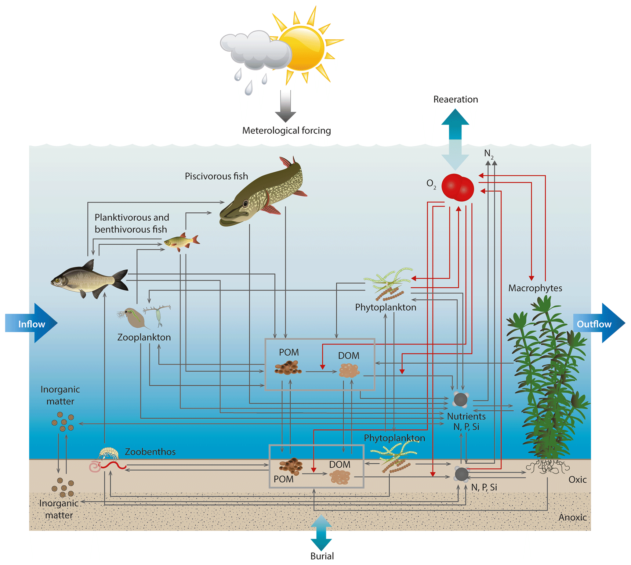
Figure 1The conceptual model of WET in a setup similar to the ones of 0D PCLake and 1D GOTM–FABM–PCLake. Grey arrows indicate fluxes of matter (dry-weight, nitrogen, phosphorous or silica) between ecosystem pools, and red arrows indicate oxygen uptake and production. Adapted from Hu et al. (2016).
Like its predecessor FABM–PCLake, WET can describe interactions between multiple trophic levels and abiotic nutrient dynamics in both the water column and the sediment. The model accounts for the dynamics of dry weight, nitrogen, phosphorous, silica and oxygen, and it features bottom-shear-dependent resuspension, as well as two different light limitation functions for phytoplankton. WET is also implemented within the FABM, allowing the model to be coupled to various physical driver models, e.g., GOTM (1D, Burchard et al., 1999) or GETM (3D, e.g., Stips et al., 2004), without changing any of the model code. Within the FABM, the physical model takes care of updating and iterating the model state variables forward in time, and the sole responsibility of the WET code is to provide local source and sink terms for its state variables as well as feedback to physical variables such as light or bottom shear stress (Bruggeman and Bolding, 2014). Here we concentrate on descriptions of the new features and all changes that separate WET from its parent model. We refer to Hu et al. (2016), Janse (2005), Janse and van Liere (1995), and Janse et al. (1992) for a detailed description of the basic equations governing the biogeochemical processes and food web dynamics, since these are unchanged, even though the model code has been rewritten and reorganized. A complete list of parameters related to the new features with options and default values can be seen in Table 1.

2.1 Modularization of the food web
A major drawback of the FABM–PCLake model is that it retains the rigid food web structure inherited from the original PCLake model and can only run in a fixed food web configuration, with fixed, preordained interactions between food web components. In contrast, WET has been designed to take full advantage of FABM by being fully modularized. This modularization enables the user to set up an arbitrary number of types of any food web element (e.g., multiple phytoplankton types) within a simulation or to remove it altogether (e.g., no fish). Thus, it is possible to customize the model to a desired level of complexity with the aim of addressing a specific study system or research question without changing any of the model code. Increasing or decreasing simulated food web complexity as the situation requires or data allows is done by simply adding or removing a food web module instance from a single configuration file (fabm.yaml, see Fig. 3). As an example, to add a new zooplankton species to an already existing model, one could first copy the lines for an existing zooplankton species in the configuration file and then change the name of the copy instance. Secondly, one would go through the couplings and parameters sections in the new zooplankton instance, modifying these to fit the desired organism. Finally, one would modify the instances of any predators to include the new zooplankton instance in their diets. Thus, adding or subtracting instances to a model setup is relatively easy, and testing for the optimal food web configuration in a specific case is possible, if not usually feasible, by calibrating several different module setups and comparing their performance.
The code base of the WET model consists of 11 Fortran files. Six of these are required files, two of which handle model initialization and shared functions, and four constitute a basic chassis of required modules, handling microbial, chemical and physical processes in the water column and upper sediment (see Fig. 2, “fixed modules”). Besides these core parts, the model consists of five optional modules representing different food web component types (phytoplankton, rooted macrophytes, zooplankton, zoobenthos and fish; see Fig. 2, “food web modules”). For all WET modules, fabm.yaml test case setup files with default parameters can be found in the test case folder of the source file repository.
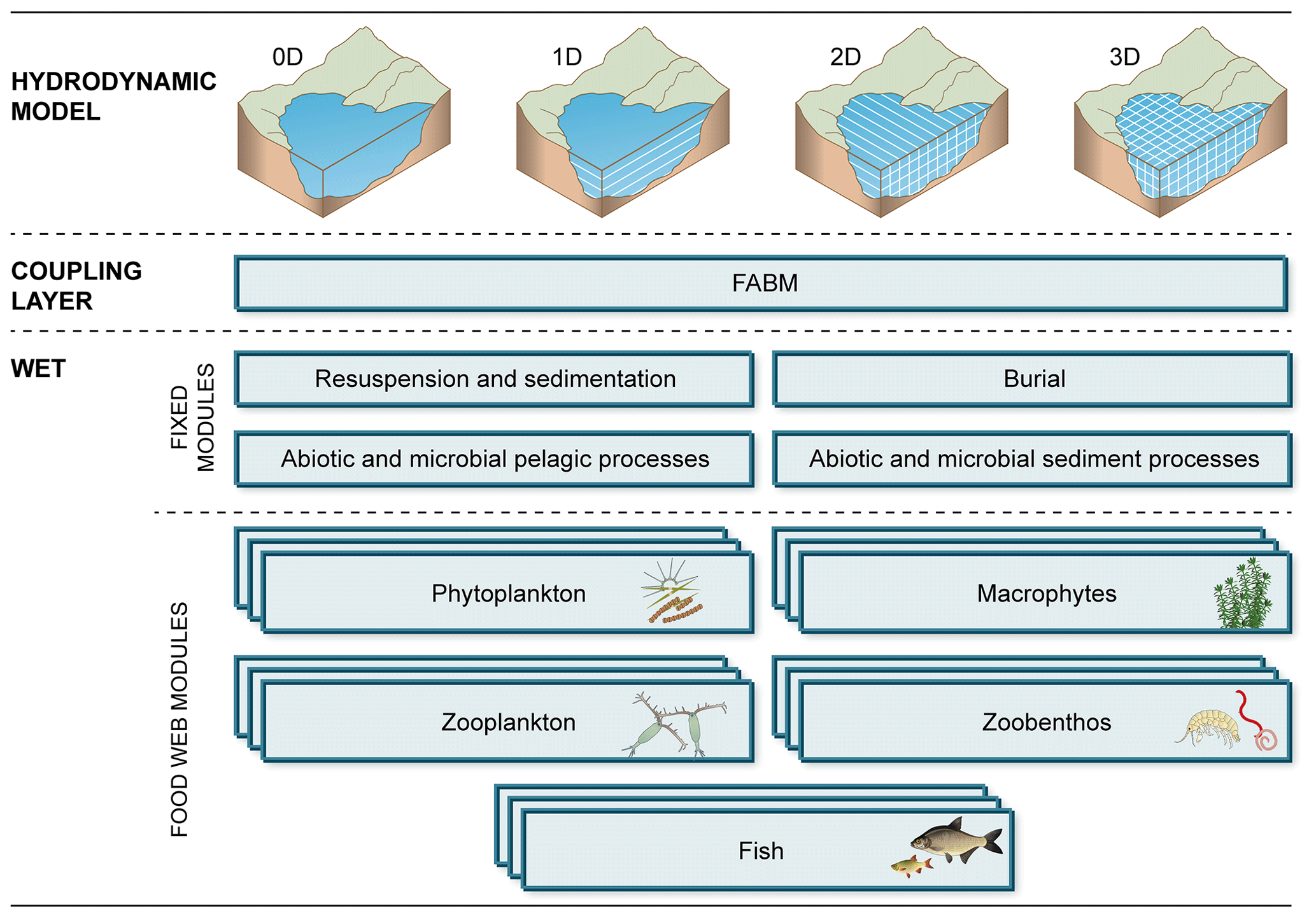
Figure 2Functional structure of a WET setup. The ecological model WET is coupled to a physical driver model (of any dimensionality) through the coupling interface FABM. WET is partitioned into a number of fixed modules, handling microbial and chemical processes, and a flexible set of fully modularized food web modules, which can be duplicated and combined as required.
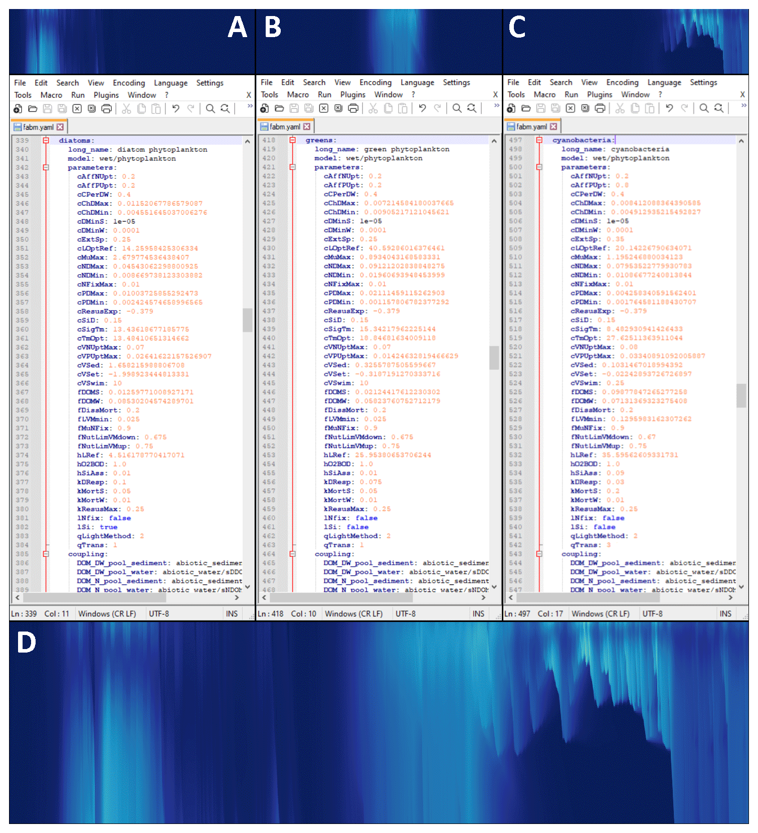
Figure 3Modular configuration of phytoplankton instances in WET. Top row: individual chlorophyll a concentrations of diatoms (a), green algae (b) and motile cyanobacteria (c). Middle row: view of the section of the model configuration file corresponding to the panel above (file opened in the open-source text editor Notepad v8.2.1). Bottom panel (d): total chlorophyll a concentration for the upper 6 m of Lake Bryrup for the year 1994, as simulated by WET coupled to the 1D GOTM lake model. Panel (d) is identical to Fig. 5e, and all axes and color maps in panels (a)–(c) are likewise identical to those of in (e), except the period shown in this figure is 1 April through 1 September.
2.1.1 Primary producers
The WET phytoplankton module is developed with a high degree of flexibility in mind and contains options to allow it to represent all main phytoplankton groups. These constitute optional dependence on silica for growth (e.g., for modeling diatoms), the option to allow phytoplankton to fix atmospheric nitrogen (e.g., cyanobacteria), and the optional ability to migrate vertically in response to ambient light and nutrient availability (various phytoplankton groups). Both nitrogen fixation and vertical movement algorithms are new features of WET, as described in the following sections (Sect. 2.2 and 2.3, respectively). The option of silica dependence is turned on by setting the parameter in the configuration file (fabm.yaml, see Fig. 3 and Table 1), and its formulation is otherwise identical to the one used in the PCLake model family (Hu et al., 2016; Janse, 2005; Janse and van Liere, 1995).
In WET, multiple types of rooted macrophytes can be included. Depending on the requirements of the modeler, all or some of the macrophyte instances can be set up to share a common carrying capacity by changing a parameter in all competing macrophyte instances and pointing to the relevant macrophyte instances in the configuration file. Aside from this option and the general modularization, the formulation of the macrophyte module is identical to FABM–PCLake (Hu et al., 2016; Janse, 2005; Janse and van Liere, 1995).
2.1.2 Heterotrophic modules
In accordance with the modularization of WET, the original feeding formulations (see Janse, 2005) of heterotrophic modules – zooplankton, zoobenthos and fish – have been adapted to be flexible, allowing predators to feed on multiple prey (including other instances of their own base module). Mixed diets are set up in the configuration file, where each prey is pointed to, and a preference factor (typically between 0 and 1) is specified following, e.g., Fasham et al. (1990). In addition, consumption of particulate organic matter (POM) is likewise an option for the invertebrate modules, i.e., zooplankton and zoobenthos.
For fish, foraging is separated into three foraging modes: planktivory, benthivory and piscivory. These foraging modes are assumed to be separate in time and/or space such that each takes up a fraction (fFishZoo, fFishBen and fFishPisc, which must sum up to 1) of the total foraging effort of the fish population. For each mode, several prey types can be present, each with their own preference factor as for zooplankton and zoobenthos. Saturation functions are calculated for each foraging mode separately using a Monod-type formulation, e.g., for piscivory,
where aDSatFiPisc is the current saturation level for piscivorous feeding, nPISC is the number of fish prey types, SDPisci is the biomass of fish prey i, PISCprefi is the preference factor for fish prey i and hDPiscFi is the half-saturation constant for piscivorous feeding. The amount of assimilated biomass from each foraging mode (here tDAssFiPisc, again using piscivory as an example) is then calculated as
where sDFi is the biomass of the predator, kDAssFi is the maximum assimilation rate of fish at 20 ∘C, aFunVegAss is the (optional) dependency of piscivory on macrophyte biomass (Janse, 2005; Janse and van Liere, 1995) and uFunTmFish is the temperature correction on fish vital rates (calculated internally in WET). The contributions from the three foraging modes are then summed for the purpose of calculating total assimilation.
2.1.3 Linking fish instances into a pseudo-stage structure
WET describes all populations in terms of biomasses and does not explicitly consider population or age structure of any organism. For fish, however, the link between juvenile (zooplanktivorous) and adult (benthivore) fish present in the PCLake model family (Hu et al., 2016; Janse, 2005; Janse and van Liere, 1995) has been generalized to the fish module. Thus, in WET, instances of the fish module can be linked through “aging” or “reproduction”, through which a fixed proportion of biomass is transferred from one instance to another on a fixed date. For both aging and reproduction, this is set up in the configuration file by setting the qStageOpt parameter, pointing to the recipient fish instance(s), and providing parameters for the date of transfer and the proportion of biomass transferred. In this way, a population of fish can be separated into a stage structure containing two, three or more stages with individual parameterizations, diets and predators. Note, however, that this implementation is not truly a stage-structured model, as each instance in the structure can in principle persist indefinitely, regardless of the state of the others.
2.2 Phytoplankton nitrogen fixation
Depending on the external nutrient inputs, nitrogen fixation by cyanobacteria can be an influential process in freshwater ecosystems (e.g., Paerl et al., 2016). Advancing from the PCLake model family (Hu et al., 2016; Janse, 2005; Janse and van Liere, 1995), WET features the possibility to simulate nitrogen fixation, which can be turned on or off by the user for each individual phytoplankton instance. This is done by setting the lNfix parameter in the configuration file (see Table 1) and supplying two additional parameters: the maximum fixation rate (cNFixMax, mgN mgDW−1 d−1) and the maximum realized fraction of the growth rate at maximum nitrogen fixation rate (fMuNfix, dimensionless). By default, total nutrient limitation for phytoplankton growth is governed by Liebig's law of the minimum and is by default calculated as
where aNutLim is the overall nutrient limitation, and aPLim, aNLim and aSiLim are the Droop functions for phosphorous, nitrogen and silica growth limitation, respectively. In the case of nitrogen fixation being turned on, nitrogen uptake rate is assumed to never limit phytoplankton growth, and consequently, total nutrient limitation is
or simply aPLim, in the absence of silica uptake. This independence of internal nutrient concentration for growth dynamics is balanced by a growth rate reduction due to allocation of energy to nitrogen fixation:
Note that this formulation assumes that nitrogen fixation takes place whenever the phytoplankton is less than nitrogen-replete (and in spite of other possible limiting nutrients) and that phytoplankton only fixes what nitrogen it cannot uptake through mineral absorption. The final nitrogen fixation rate is calculated as
and has units of mg N mg−1 DW d−1. This formulation of the nitrogen fixation dynamics in WET is adapted from the CAEDYM model (Hamilton and Schladow, 1997; CAEDYM team, 2019), while this general formulation of nitrogen fixation is common in phytoplankton models (see, e.g., Inomura et al., 2020, and references therein).
2.3 Vertical movement algorithms
In WET, all pelagic food web modules (i.e., phytoplankton, zooplankton and fish) now have several options for vertical migration. The purpose of these options is to (1) add flexibility to the types of environment that can be modeled with WET and (2) to increase model accuracy and applicability by providing more realistic dynamics of all food web elements in all types of aquatic systems. The various options for vertical migration are presented for each model element below. These options can be configured individually for each instance at runtime by setting the qTrans parameter and any necessary additional option-specific parameters.
2.3.1 Phytoplankton module
The WET phytoplankton module contains four modes of vertical movement behavior: passive transport (no active movement), passive transport plus active chemotaxis (for nutrients), passive transport plus active phototaxis, and passive transport plus combined phototaxis and chemotaxis (see Table 1 for details on options and parameterization). The VM functions of phytoplankton described below are all based on Ross and Sharples (2007).
The first vertical movement option is passive transport, which is identical to what is currently the only available mode in FABM–PCLake, wherein phytoplankton only move vertically as a result of passive advection by the host physical model as well as through a fixed sinking rate (positive, negative or neutral buoyancy). The fixed sinking rate is specified through the cVSet parameter and is negative in the case of sinking.
In addition to passive advection, when chemotaxis is turned on, phytoplankton will swim downwards with constant swimming speed whenever the nutrient limitation growth coefficient decreases below a threshold value. Thus, phytoplankton in WET operate under the assumption that nutrient concentrations are always higher at greater depth.
When phototaxis is turned on, phytoplankton will swim upwards with fixed speed whenever ambient light levels surpass a light threshold value.
The fourth phytoplankton vertical movement option combines chemotaxis and phototaxis such that chemotaxis takes precedence over phototaxis. Thus, phytoplankton will swim down in nutrient-depleted situations and up when the cell is nutrient-replete, provided that ambient light levels surpass the threshold value.
2.3.2 Zooplankton and fish modules
Regular vertical movements between different depths are a common behavior in both fish and zooplankton populations, especially in deeper systems. Such movement behavior is expressed for a variety of reasons, including avoidance of hypoxic regions, predator avoidance, and bioenergetic exploitation of gradients in temperature or food availability (Dini and Carpenter, 1992; Dodson, 1990; Lambert, 1989; Mehner, 2012).
An inherent limitation to the FABM is that modules are limited in the amount of information they receive about conditions outside the current model cell, e.g., food availability at other depths. Thus, modeled motile organisms are limited to making “decisions” about movement based on either local conditions or predictable environmental gradients. Due to this limitation, directional vertical movements of zooplankton and fish in WET are restricted to being in response to hypoxia, ambient light levels or both. The WET zooplankton and fish modules contain four modes of vertical migration behavior: no transport (no transport between layers, even advection), passive transport (no active transport), hypoxia avoidance, and light-based diel vertical migration combined with hypoxia avoidance. Of these, the “no transport” option turns off all exchange between model layers (only relevant in > 0D applications) and is mainly a debugging or analytical tool.
As for phytoplankton, when vertical movement is set to passive transport, fish and zooplankton are passively advected by the physical model.
Hypoxia avoidance restricts the habitat domain to exclude anoxic parts of the water column, which is a ubiquitous response to hypoxia among zooplankton and fish (Ekau et al., 2010; Vanderploeg et al., 2009). When hypoxia avoidance is turned on for a WET module, fish or zooplankton swim upwards whenever the ambient oxygen concentration falls below the critical threshold in the current model cell.
Zooplankton and fish may employ diel vertical migration for a number of reasons (Dini and Carpenter, 1992; Dodson, 1990; Lambert, 1989; Mehner, 2012; Sainmont et al., 2013), but ambient light levels are often the proximate trigger for this behavior. Under this setting, in addition to passive advection and hypoxia avoidance, fish or zooplankton will swim downwards whenever light exceeds a maximum level and upwards whenever light decreases below the lower light threshold. Either the downwards or upwards portions of this movement can be turned off by setting the maximum (minimum) threshold to a very high (negative) value.
To illustrate some of the new features in the WET model, we applied the GOTM–WET model for Lake Bryrup, for which a calibration of the FABM–PCLake model (coupled to the lake version of the 1D hydrodynamic model GOTM, Burchard et al., 1999) was previously published by Chen et al. (2020). Here we have adapted, recalibrated and validated this setup using WET, following the methodology and approaches of Chen et al. (2020), and use the results to illustrate some of the new features of WET and how these can impact the model behavior.
3.1 Study site and model configuration
The shallow Lake Bryrup is located in the central region of Denmark (56.02∘ N, 9.53∘ E) and has a surface area of 37 ha, a mean depth of 4.6 m and a maximum depth of 9 m. The lake stratifies temporarily during summer and has a water retention time of 2–3 months. The catchment area is 49.9 km2 and heavily farmed, and the lake receives large amounts of nutrients from agricultural and urban drainage (Johansson et al., 2019). Consequently, the lake is eutrophic although management measures have been effective in reducing average total nitrogen and phosphorous concentrations throughout the last decades (see Chen et al., 2020, for a more thorough description of Lake Bryrup).
As the chosen physical driver model for the Lake Bryrup test case, we used the Aarhus University fork of lake branch GOTM (version 5.2.2-au, available at https://gitlab.com/WET/gotm, last access: 11 May 2022), configured with a maximum depth of 9.0 and 18 vertical layers (i.e., vertical grid size of 0.5 m). In order produce high-resolution output for the present figures, the model was also run with 200-layer resolution. The setup used a lake-specific hypsograph (i.e., the relation between depth and horizontal area) to capture lake sediment–water column interactions at all depths by effectively splitting the bottom between model layers such that each model layer in the 1D setup has an attached bottom layer. Interactions between the water column of a layer, its attached bottom and the water column layer below are governed by the hypsograph, which specifies the fraction of the bottom area to total layer area. The setup therefore in some aspects functions as a pseudo-2D setup. Each model layer thus included a sediment layer of 10 cm, similar to the sediment compartment of the PCLake model. See Andersen et al. (2020) and Hu et al. (2016) for detailed descriptions of these aspects of the model. To simulate lake ice thickness and cover, implementation in GOTM of the ice module from MyLake (Saloranta and Andersen, 2007) was enabled. In WET, the food web comprised three phytoplankton groups (diatoms, cyanobacteria and other algae), rooted submerged macrophytes, two zooplankton groups (Daphnia and other zooplankton), detritivorous macrozoobenthos, juvenile zooplanktivorous, and adult zoobenthivorous fish and piscivorous fish (Fig. 1). We applied the European ECMWF ERA5 dataset (Hersbach et al., 2018) at an hourly resolution for air temperature (∘C), air pressure (hPa), dew-point temperature (∘C), cloud cover (%) and wind speed components (m s−1) in the north–south and west–east direction as meteorological forcing for GOTM. Monthly averages of water inflow (m3 s−1) and nutrient concentrations (NO3, NH4, PO4, and particulate organic matter of nitrogen and phosphorous, mg L−1) from the National Monitoring and Assessment Program for the Aquatic and Terrestrial Environment in Denmark (NOVANA) (Jørgensen et al., 2007) were used as boundary conditions (see Chen et al., 2020, for details), applied in the topmost model layer (both inflow and outflow). The model was executed with an hourly time step and daily (midday) output of model results, except for the high-resolution runs, which ran with a 10 min time step and output.
3.2 Model calibration and validation
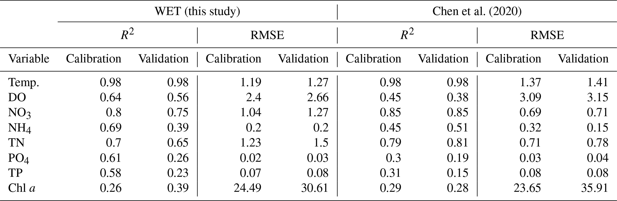
The GOTM–WET model for Lake Bryrup was calibrated following the calibration procedure described in Chen et al. (2020), which applied the autocalibration tool parsac (Bruggeman and Bolding, 2020) with 6 spin-up years to initialize biogeochemical nutrient pools, a calibration period of 8 years (1996–2004) and a validation period of 2 years (2004–2006). Model results were compared against monthly to semi-monthly data for water temperature (∘C), dissolved oxygen (mg L−1), inorganic nutrient concentrations (NO3, NH4 and PO4, mg L−1), total nitrogen and phosphorous concentrations (TN and TP, mg L−1), and chlorophyll a concentrations (chl a, µg L−1) obtained from the NOVANA program available at http://www.miljoportal.dk (lst access: 11 May 2022). Spatial resolution of the in-lake dataset for calibration and validation varied with 1–12 measurements per sample date across the water column for water temperature and DO (median of 7 measurements per date) and 1–3 samples per date for water nutrient concentrations (median of 2). All chl a concentrations were sampled in the surface (between 0 and 3 m depth) once per sample date. We evaluated model performance by computing the root mean square error (RMSE) and coefficient of determination (R2) for the daily output of each state variable. Model results have been processed and visualized in Python with the packages xarray version 0.15.1 (Hoyer and Hamman, 2017), Matplotlib version 3.1.2 (Hunter, 2007) and seaborne version 0.11.1 (Waskom, 2021), as well as with the open-source Python program PyNcView (available via The Python Package Index, pip install pyncview).
The new WET version of Lake Bryrup model differs from the FABM–PCLake version in a few areas, first and foremost by taking advantage of the new options for vertical mobility for motile cyanobacteria and zooplankton, as well as by allowing dispersion of fish between layers (see Sect. 2.3). In addition, the new modularization has allowed us try out an alternate food web configuration, namely the differentiation of zooplankton into two boxes (mesozooplankton and Daphnia), although in this instance we are limited by the availability of data for calibration.
The new model yields performance metrics that are overall comparable to or slightly improved compared to the ones obtained by Chen et al. (2020), with slightly lower or equal performance statistics for oxygen and nitrogen state variables but improved performance for phosphorous, chlorophyll a and temperature (see Table 2).
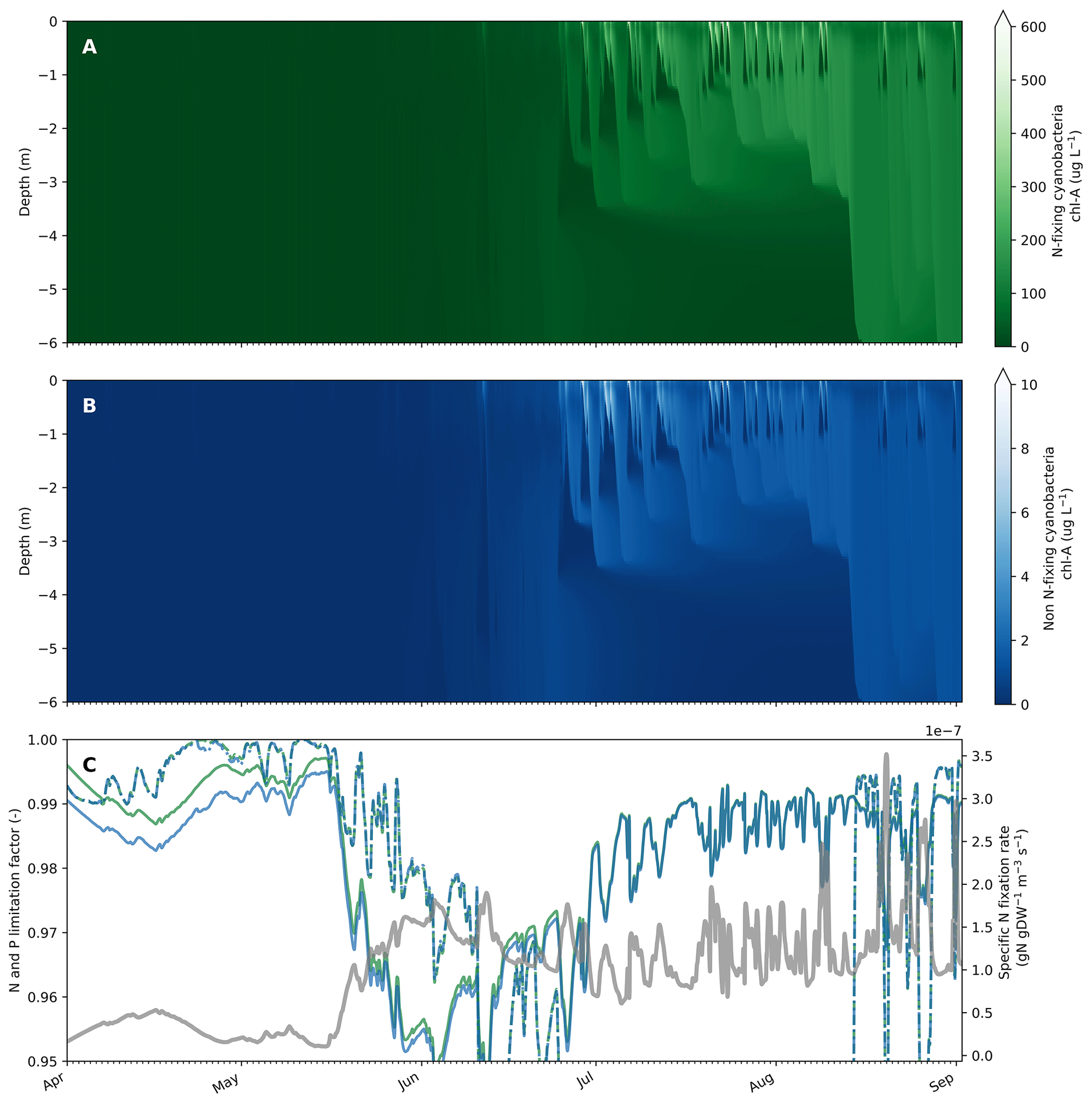
Figure 4Example of simulated cyanobacteria, nutrient limitation and N fixation dynamics in Lake Bryrup from April to September 1994. Output of N-fixing and non-N-fixing cyanobacteria chl a concentrations from the upper 6 m of Lake Bryrup (a, b). C:N and P limitation factor (solid and dashed lines, respectively) for N-fixing and non-N-fixing cyanobacteria (green and blue lines, respectively) as well as the specific N fixation rate by N-fixing cyanobacteria (grey line, secondary y axis) in the surface model layer (surface to 0.5 m). The phytoplankton group is nutrient-replete (N and/or P) or nutrient-depleted when the limitation factor is equal to 1 or 0, respectively.
Table 2Comparison of performance metrics between Chen et al. (2020) and the present study.
Figures 3–5 illustrate select dynamics from the Lake Bryrup WET model. For these figures, the calibrated model was rerun at a higher resolution in time and space relative to the base calibration in order to increase visual detail of spatial and temporal dynamics. The obtained high-resolution results were similar to the dynamics of model runs with lower resolution.
4.1 Phytoplankton modularity
As in Chen et al. (2020), the WET recalibrated Lake Bryrup model contains three phytoplankton groups: diatoms, green algae and cyanobacteria (Fig. 3). The general seasonal phytoplankton succession in Lake Bryrup involves a spring diatom bloom, an early summer bloom of green algae, and a cyanobacteria bloom in late summer or when the water column stratifies for a prolonged period. The central panels in Fig. 3 illustrate the separation of multiple phytoplankton groups into separate versions of the same general module, making it easy to add, switch out or remove phytoplankton groups from the model and to parameterize these individually. The chosen set of phytoplankton categories reflects the available data and matches the previous FABM–PCLake version of the model.
4.2 Phytoplankton nitrogen fixation
To illustrate the interplay and dynamics between nutrient limitation, nitrogen fixation and growth of cyanobacteria with and without nitrogen fixation ability, we included an additional cyanobacteria group with parameters identical to the calibrated cyanobacteria group besides N fixation turned on with default values (lNfix = true and fMuNFix = 0.9). Although phytoplankton groups in Lake Bryrup are P-limited in the period during which cyanobacteria blooms frequently occur (approximately mid-June to mid-August with simulated P limitation between 0.8 and 0.5), N-fixing cyanobacteria dominated the community in contrast to the non-N-fixing cyanobacteria (Fig. 4a and b). Both cyanobacteria groups were N-limited in spring, which allowed N-fixing cyanobacteria to get an advantage by decreasing N limitation via N fixation (Fig. 4c) and increase biomass concentrations, thereby having a head start for the period with low mixing and warmer surface waters. As expected, N fixation rates increased with increased N limitation and N fixation. The cyanobacteria biomass concentration is shown in Fig. 4c (secondary y axis). The relatively low N limitation experienced by the N-fixing cyanobacteria group (N limitation factor between 0.95 and 1.0) resulted in a low growth rate penalty during periods with N fixation between 0 % and 1.5 %. In scenarios with altered external nutrient loads switching from a P-limited to an N-limited system in late summer to fall, N-fixing cyanobacteria still dominate the phytoplankton community in late summer with N fixation rates now significantly increased (for instance, 20-fold in one scenario) as the cyanobacteria are now more N-limited.
4.3 Phytoplankton vertical mobility
Figure 5 illustrates the new options for modeling vertical movement for phytoplankton in WET, with panel (a) illustrating water column temperature, panel (b) illustrating overall nutrient conditions (for cyanobacteria) in the water column, and panels (c)–(f) illustrating the dynamics associated with each of the four vertical movement settings (here only for cyanobacteria). Of these, panel (c) corresponds to the old FABM–PCLake condition (Hu et al., 2016). Much of the seasonal succession of phytoplankton, especially the shift from denser-than-water and non-motile phytoplankton (pre-July dynamics in Fig. 5c–f, see also Fig. 3a and b) to a mid-to-late-summer cyanobacterial bloom, is driven mainly by the presence or absence and location of lake stratification (as indicated by the temperature gradients in Fig. 5a). The early part of the growing season is dominated by relatively fast-sinking non-motile diatoms and green algae, which have qTrans set to 1 (passive advection and fixed sinking rate, see Sect. 2.3.1) in the configuration file (Fig. 3).

Figure 5Output from the upper 6 m of Lake Bryrup for the year 1994, as simulated by WET coupled to the 1D GOTM lake model. (a) Water temperature. (b) Overall nutrient limitation factor for the cyanobacteria instance. (c, f) Total water column chlorophyll a for different settings of cyanobacterial vertical movement. (c) Passive movement (qTrans = 1). (d) Nutrient taxis (qTrans = 2). (e) Phototaxis (qTrans = 2). (f) Combined phototaxis and nutrient taxis. For all panels, the cyanobacterial swimming speed, cVSwim, was set to 0.25 m d−1. The other vertical movement parameters were set to fNutLimVMdown = 0.67, fNutLimVMup = 0.75 and fLVMmin = 0.13 W m2. For (c)–(f), note the fully mixed diatom bloom in spring, followed by a summer bloom of cyanobacteria in late summer. For legibility of the figure, the maximum color bar cutoff for (c)–(f) has been set at a lower value than brief and localized very high chlorophyll a concentrations (up to ∼ 1300 µg L−1 in f).
With the formation of a late summer stable stratification, relatively buoyant or motile cyanobacteria (Figs. 3c, 5c–f) become dominant, in part due to their ability to stay in the epilimnion. Even under the passive transport setting (Fig. 5c), cyanobacteria are able to sustain a bloom under stratified conditions due to their slow sinking rate (cVSet = −0.022 m d−1). However, when phototaxis is turned on (Fig. 5e), higher biomasses are reached by the cyanobacteria. When nutrient taxis without phototaxis is turned on (Fig. 5d), cyanobacteria aggregate at the bottom of the mixed layer when nutrients at the surface are very scarce (Fig. 5b). Under the combined nutrient and phototaxis setting (Fig. 5f), cyanobacteria aggregate around the bottom of the thermocline, forming a deep chlorophyll maximum (DCM), where nutrients are more available and cyanobacteria are less nutrient-limited (i.e., higher simulated nutrient limitation factor) but are also able to exploit higher light intensities at the surface, resulting in higher biomasses compared with nutrient taxis alone.
4.4 Zooplankton vertical mobility
In WET, heterotrophic pelagic modules such as fish and zooplankton can exhibit vertical movement in the form of hypoxia avoidance behavior and light-triggered diel vertical migration (see Sect. 2.3.2). Figure 6 illustrates the three options for zooplankton and fish vertical mobility behavior in WET. Triggered by the upwards and downwards migration of the hypoxic deep zone (Fig. 6d) and the daily light cycle (Fig. 6f), the Daphnia in Fig. 6a conduct diel vertical migrations when qTrans is set to 3. The active movement of zooplankton is modulated by advection (Fig. 6e), which diffuses part of the migrating zooplankton during days of high turbulent mixing (e.g., on 3 and 7 July in Fig. 6). In panel (b) in Fig. 6 (qTrans = 2), upwards swimming is triggered when hypoxic conditions extends up into the water column, which does not happen when vertical movement of Daphnia is limited to passive advection (panel c in Fig. 6, qTrans = 1).

Figure 6Example of simulated vertical migration in WET. Output from the upper 6 m of Lake Bryrup during 5 d in July 1994, as simulated by WET coupled to the 1D GOTM lake model. (a) Vertical distribution of Daphnia dry-weight biomass, with vertical movement set to light-based vertical movement. Note the vertical movements of zooplankton biomass, triggered by light intensity in the water column, as well as oxygen depletion in the hypolimnion and modulated by turbulent mixing. (b) Vertical distribution of Daphnia dry-weight biomass, with vertical movement set to hypoxia avoidance. (c) Vertical distribution of Daphnia dry-weight biomass, with vertical movement set to passive transport only. (d–f) Oxygen, turbulent and light conditions, respectively, which inform the vertical movement of zooplankton. For legibility of the figure, the maximum color bar cutoff has been set at a lower value than brief and localized very high Daphnia concentrations (∼ 30 g m−3) during the anoxia avoidance episodes. (b) Downwelling shortwave radiation. For these simulations, Daphnia vertical movement parameters were set to Vswim = 45 m d−1, cMaxLight = 40.0 W m−2, cMinLight = 0.15 W m−2 and cMinO2 = 2.0 g O2 m−3.
5.1 Observations on the performance of the new vertical movement and nitrogen fixation features
Model configuration and complexity are often constrained by data availability. Symptomatically, although Lake Bryrup is included in the Danish long-term ecological monitoring program (NOVANA), there are no data against which to validate, for instance, spatial distributions of higher organisms. Here, we have been mostly concerned with demonstrating the features of WET, but the ability to model diel vertical migration (DVM) will be essential in many applications worldwide, especially large and deep lakes across the globe, as well as in many marine or estuarine environments. In such cases the modeler will often have to rely on studies that specifically target zooplankton (or fish) DVM in similar environments. For fish, however, a large step (if somewhat of a low-hanging fruit) towards more realistic model representation has been taken in WET, with the removal of the unrealistic absence of movement between model layers in its predecessor FABM–PCLake model.
While DVM in zooplankton and fish is an elusive dynamic to observe and understand, the importance of vertical movement processes for the composition and seasonal succession of phytoplankton communities is more easily recognized. Motile phytoplankton have a distinct advantage in highly stratified conditions in which the ability to stay in the euphotic epilimnion (Wentzky et al., 2020), or to balance opposing gradients of light and nutrients by migrating to the hypolimnion (Leach et al., 2018), can be important. We demonstrated that the choice of DVM method has profound impacts on model behavior (Fig. 5), e.g., whether mobile phytoplankton will concentration at the surface layer or near the bottom of the thermocline (i.e., forming a DCM).
The option of nitrogen fixation in phytoplankton is another feature which might improve model performance in stratified or oligotrophic lakes, where nitrogen limitation can be important (Reinl et al., 2021), although the ability of N fixation to fully compensate for nitrogen limitation has recently been called into question (Shatwell and Köhler, 2019). In the present study, the impact of nitrogen fixation was expected to be low, as Lake Bryrup is predominantly limited by phosphorous, particularly in the main part of the growing season. Nevertheless, by adding a nitrogen-fixing cyanobacterial competitor, we shoved how shifting nutrient conditions throughout the growth season shaped the relative competitive landscape, as well as the nitrogen fixation rate of the N-fixing cyanobacteria throughout the model period.
5.2 Advantages of model modularization
As demonstrated here, the WET model can reproduce the behavior of FABM–PCLake. But this food web configuration might not be optimal for every, nor even necessarily in this, use case. While beyond the scope of this paper, the WET model application to Lake Bryrup could potentially be calibrated in several food web configurations to find the optimum conceptual representation. This procedure could in principle be applied in all model applications as an extra layer in the calibration process, but it will not be feasible in many cases in the face of the already daunting task of calibrating a model with hundreds of parameters. Unfortunately, we believe that this is a case in which there is no replacement for experience with both models and the study system, and scientists will have to rely on their expertise to configure the most accurate and realistic food web for any given research question. However, on a smaller scale, it will often be possible to test different food web compositions by, e.g., adding or subtracting an extra phytoplankton, zooplankton or fish module to an already calibrated model and doing simpler recalibrations.
Differences in ecosystem structure and functions between lakes in different climatic regions would also most likely warrant changes to food web configurations. For example, fish populations in (sub)tropical shallow lakes generally have a smaller body size, shorter life span, faster growth, multiple reproduction events and stronger preference for the littoral zone compared to temperate lakes (Meerhoff et al., 2012, and references therein). In combination with an increased proportion of herbivorous and omnivorous fish species (González-Bergonzoni et al., 2012; Iglesias et al., 2017), this difference would most likely weaken trophic cascades and thereby diminish the impact of several lake restoration strategies (Jeppesen et al., 2010). So to reproduce, for instance, warm water shallow lake dynamics and responses to potential restoration efforts, configuration of the food web to the specific lake is likely needed.
5.3 Concluding remarks regarding the new features
Overall, the new changes that separate WET from its predecessors provide the model with a high degree of flexibility and adaptability, with the distinct advantage of allowing one model code base to handle many different application cases instead of requiring many distinct models for different purposes. By taking advantage of the modularization, distinct food web configurations can be set up for different systems. Meanwhile, the new vertical movement and nitrogen fixation algorithms allow the model to be applicable in a much wider array of physical settings and across gradients in latitude, depth or salinity. This flexibility of the new model may contribute to limiting cases of parallel development and “re-inventing the wheel”, while promoting comparability between different model implementations. As stated in the Introduction, we believe that the consolidation of various model features and approaches into a few flexible and customizable models is a crucial process for the overall progress of the field of ecological modeling. However, for such models to be truly and successfully flexible, such customization must be possible with relative ease or risk going unused. The modularized structure of WET under the FABM supports the user by making everything configurable in a single setup file, by making it easy to switch modules on or off, and by having all options relevant to an organism type available from the base module. By switching out module sections or an entire configuration file, a new model setup can be run with the same executable without having to change or recompile any source code. For an even simpler workflow, running the model through the QWET plugin for the QGIS software provides the user with a simple step-by-step GUI-based process, for which a tutorial is available on the WET home page.
5.4 Future work
WET is under active and continuous development. Currently, effort is being applied to improve the applicability of the model to subtropical and tropical regions, which will include improvements to the macrophyte module and support for herbivory in fish. Another work in progress is a complete overhaul of the heterotrophic modules, replacing old feeding formulations with more realistic descriptions, and introducing options for dynamic diets, feeding strategies and foraging efforts of fish based on optimal foraging theory.
Apart from these new features, other areas for future work include improved handling of resuspension of sediment, a fully size-based fish module, and extensive testing and improvements of the model in a 3D application, with the expressed aim of the authors (in their roles as the current main developers of WET) that the model be even more tailorable to a wide array of ecosystem types across latitudinal, spatial and productivity gradients simply by turning features on or off and combining different modules that are all configurable at runtime. With this model, which is open-source and freely available, we hope to facilitate the consolidation of successful features of many models together in one, with the goal of preventing “re-inventions of the wheel” in the future and making aquatic ecosystem modeling easier, more flexible and, ultimately, better.
Name of software: WET (Water Ecosystems Tool) – version 1.0
Developers: Dennis Trolle, Fenjuan Hu, Nicolas Azaña Schnedler-Meyer, Tobias Kuhlmann Andersen, Karsten Bolding and Anders Nielsen
Contact Address: Department of Bioscience, Aarhus University, Vejlsøvej 25, 8600 Silkeborg, Denmark
Email: wet.info@wet.au.dk
Availability: freely available under the GNU General Public License (GPL) version 2. Further information, executables and source code are available at http://wet.au.dk (last access: 11 May 2022), https://gitlab.com/WET (last access: 11 May 2022) or https://doi.org/10.5281/zenodo.6482852 (Schnedler-Meyer et al., 2022). A guide for model compilation, setup and configuration is available at the WET website (see “For developers”). Follow this guide in order to download and compile the model.
This paper utilized data from the Copernicus Climate Change Service information 2020. Hersbach et al. (2018, https://doi.org/10.24381/cds.adbb2d47) was downloaded from the Copernicus Climate Change Service (C3S) Climate Data Store.
In addition, data from the National Monitoring and Assessment Program for the Aquatic and Terrestrial Environment in Denmark (NOVANA) were used (Jørgensen et al., 2007; Johansson et al., 2019). The data are stored in the ODA database and can be accessed through the“ODA for alle” data portal (https://odaforalle.au.dk/, last access: 11 May 2022). The data were downloaded on 1 January 2020. These data were used in accordance with the principles for the use of Danish public data.
The model was coded and developed mainly by NASM, with significant contributions and aid from DT, TKA, FRSH and KB, based on a previous model code by FRSH. The test case was adapted and carried out by TKA, and NASM prepared the paper with contributions from all co-authors.
The contact author has declared that neither they nor their co-authors have any competing interests.
Neither the European Commission nor ECMWF is responsible for any use that may be made of the Copernicus information or data it contains.
Publisher's note: Copernicus Publications remains neutral with regard to jurisdictional claims in published maps and institutional affiliations.
The authors would like to thank Jorn Bruggemann for extensive support related to the inner workings of FABM.
This development has been supported by the CASHFISH project funded by the Danish Council for Independent Research, the WATExR project funded through the EU JPI Climate initiative, the PROGNOS project funded through the EU JPI Water initiative, the project Mechanistic Models for Water Action Planning funded by the Danish EPA, and the Lake Stewardship Project supported by the Poul Due Jensen Foundation. Tobias Kuhlmann Andersen was supported by PhD funding from the Sino-Danish Center for Education and Research.
This paper was edited by Andrew Yool and reviewed by Xiangzhen Kong and one anonymous referee.
Allan, M.: Ecological modelling of water quality management options in Lake Waahi to support Hauanga Kai species: Technical report, Hamilton, New Zealand, 2018.
Andersen, T. K., Nielsen, A., Jeppesen, E., Hu, F., Bolding, K., Liu, Z., Søndergaard, M., Johansson, L. S., and Trolle, D.: Predicting ecosystem state changes in shallow lakes using an aquatic ecosystem model: Lake Hinge, Denmark, an example, Ecol. Appl., 30, 1–21, https://doi.org/10.1002/eap.2160, 2020.
Arnold, J. G., Srinivasan, R., Muttiah, R. S., and Williams, J. R.: Large area hydrologic nodeling and assessment part 1: model development, J. Am. Water Resour. Assoc., 34, 73–89, 1998.
Bruggeman, J. and Bolding, K.: A general framework for aquatic biogeochemical models, Environ. Model. Softw., 61, 249–265, https://doi.org/10.1016/j.envsoft.2014.04.002, 2014.
Bruggeman, J. and Bolding, K.: parsac: parallel sensitivity analysis and calibration, Zenodo [code], https://doi.org/10.5281/ZENODO.4280520, 2020.
Burchard, H., Bolding, K., and Villarreal, M.: GOTM, a general ocean turbulence model: Theory, implementation and test cases, Tech Rep EUR 18745 EN European Commission, 1999.
CAEDYM team: CAEDYM (Computational Aquatic Ecosystem DYnamics Model), Model Item, OpenGMS, https://geomodeling.njnu.edu.cn/modelItem/3dcb8f17-95ed-4e5e-aa7b-3efa7ed61add (last access: 11 May 2022), 2019.
Chen, W., Nielsen, A., Andersen, T. K., Hu, F., Chou, Q., Søndergaard, M., Jeppesen, E., and Trolle, D.: Modeling the ecological response of a temporarily summer-stratified lake to extreme heatwaves, Water (Switzerland), 12, 1–17, https://doi.org/10.3390/w12010094, 2020.
Dini, M. L. and Carpenter, S. R.: Fish predators, food availability and diel vertical migration in Daphnia, J. Plankton Res., 14, 359–377, https://doi.org/10.1093/plankt/14.3.359, 1992.
Dodson, S.: Predicting diel vertical migration of zooplankton, Limnol. Oceanogr., 35, 1195–1200, https://doi.org/10.4319/lo.1990.35.5.1195, 1990.
Ekau, W., Auel, H., Pörtner, H.-O., and Gilbert, D.: Impacts of hypoxia on the structure and processes in pelagic communities (zooplankton, macro-invertebrates and fish), Biogeosciences, 7, 1669–1699, https://doi.org/10.5194/bg-7-1669-2010, 2010.
Fasham, M. J. R., Ducklow, H. W., and McKelvie, S. M.: A nitrogen-based model of plankton dynamics in the oceanic mixed layer, J. Mar. Res., 48, 591–639, https://doi.org/10.1357/002224090784984678, 1990.
González-Bergonzoni, I., Meerhoff, M., Davidson, T. A., Teixeira-de Mello, F., Baattrup-Pedersen, A., and Jeppesen, E.: Meta-analysis Shows a Consistent and Strong Latitudinal Pattern in Fish Omnivory Across Ecosystems, Ecosystems, 15, 492–503, https://doi.org/10.1007/s10021-012-9524-4, 2012.
Hamilton, D. P. and Schladow, S. G.: Prediction of water quality in lakes and reservoirs, Part I – Model description, Ecol. Modell., 96, 91–110, 1997.
Hersbach, H., Bell, B., Berrisford, P., Biavati, G., Horányi, A., Muñoz Sabater, J., Nicolas, J., Peubey, C., Radu, R., Rozum, I., Schepers, D., Simmons, A., Soci, C., Dee, D., and Thépaut, J.-N.: ERA5 hourly data on single levels from 1979 to present, Copernicus Climate Change Service (C3S) Climate Data Store (CDS) [data set], https://doi.org/10.24381/cds.adbb2d47, 2018.
Hoyer, S. and Hamman, J. J.: xarray: N-D labeled Arrays and Datasets in Python, J. Open Res. Softw., 5, 1–6, https://doi.org/10.5334/jors.148, 2017.
Hu, F., Bolding, K., Bruggeman, J., Jeppesen, E., Flindt, M. R., van Gerven, L., Janse, J. H., Janssen, A. B. G., Kuiper, J. J., Mooij, W. M., and Trolle, D.: FABM-PCLake – linking aquatic ecology with hydrodynamics, Geosci. Model Dev., 9, 2271–2278, https://doi.org/10.5194/gmd-9-2271-2016, 2016.
Hunter, J. D.: Matplotlib: A 2D Graphics Environment, Comput. Sci. Eng., 9, 90–95, https://doi.org/10.1109/MCSE.2007.55, 2007.
Iglesias, C., Meerhoff, M., Johansson, L. S., González-Bergonzoni, I., Mazzeo, N., Pacheco, J. P., Mello, F. T. de, Goyenola, G., Lauridsen, T. L., Søndergaard, M., Davidson, T. A., and Jeppesen, E.: Stable isotope analysis confirms substantial differences between subtropical and temperate shallow lake food webs, Hydrobiologia, 784, 111–123, https://doi.org/10.1007/s10750-016-2861-0, 2017.
Inomura, K., Deutsch, C., Masuda, T., Prášil, O. and Follows, M. J.: Quantitative models of nitrogen-fixing organisms, Comput. Struct. Biotechnol. J., 18, 3905–3924, https://doi.org/10.1016/j.csbj.2020.11.022, 2020.
Janse, J. H.: A model of nutrient dynamics in shallow lakes in relation to multiple stable states, in: Shallow Lakes '95: Trophic Cascades in Shallow Freshwater and Brackish Lakes, edited by: Kufel, L., Prejs, A., and Rybak, J. I., Springer Netherlands, Dordrecht, 1–8, 1997.
Janse, J. H.: Model studies on the eutrophication of shallow lakes and ditches, Book, Wageningen University and Research, ISBN 90-8504-214-3, 2005.
Janse, J. H. and Aldenberg, T.: Modelling phosphorus fluxes in the hypertrophic Loosdrecht Lakes, Hydrobiol. Bull., 24, 69–89, https://doi.org/10.1007/BF02256750, 1990.
Janse, J. H. and van Liere, L.: PCLake: A modelling tool for the evaluation of lakes restoration scenarios, Water Sci. Technol., 31, 371–374, 1995.
Janse, J. H., Aldenberg, T., and Kramer, P. R. G.: A mathematical model of the phosphorus cycle in Lake Loosdrecht and simulation of additional measures, Hydrobiologia, 233, 119–136, https://doi.org/10.1007/BF00016101, 1992.
Janssen, A. B. G., Arhonditsis, G. B., Beusen, A., Bolding, K., Bruce, L., Bruggeman, J., Couture, R.-M., Downing, A. S., Elliott, J. A., Frassl, M. A., Gal, G., Gerla, D. J., Hipsey, M. R., Hu, F., Ives, S. C., Janse, J. H., Jeppesen, E., Jöhnk, K. D., Kneis, D., Kong, X., Kuiper, J. J., Lehmann, M. K., Lemmen, C., Özkundakci, D., Petzoldt, T., Rinke, K., Robson, B. J., Sachse, R., Schep, S. A., Schmid, M., Scholten, H., Teurlincx, S., Trolle, D., Troost, T. A., Dam, A. A. Van, Van Gerven, L. P. A., Weijerman, M., Wells, S. A., and Mooij, W. M.: Exploring, exploiting and evolving diversity of aquatic ecosystem models: a community perspective, Aquat. Ecol., 49, 513–548, https://doi.org/10.1007/s10452-015-9544-1, 2015.
Janssen, A. B. G., Teurlincx, S., Beusen, A. H. W., Huijbregts, M. A. J., Rost, J., Schipper, A. M., Seelen, L. M. S., Mooij, W. M., and Janse, J. H.: PCLake+: A process-based ecological model to assess the trophic state of stratified and non-stratified freshwater lakes worldwide, Ecol. Modell., 396, 23–32, https://doi.org/10.1016/j.ecolmodel.2019.01.006, 2019.
Jeppesen, E., Meerhoff, M., Holmgren, K., González-Bergonzoni, I., Teixeira-de Mello, F., Declerck, S. A. J., De Meester, L., Søndergaard, M., Lauridsen, T. L., Bjerring, R., Conde-Porcuna, J. M., Mazzeo, N., Iglesias, C., Reizenstein, M., Malmquist, H. J., Liu, Z., Balayla, D., and Lazzaro, X.: Impacts of climate warming on lake fish community structure and potential effects on ecosystem function, Hydrobiologia, 646, 73–90, https://doi.org/10.1007/s10750-010-0171-5, 2010.
Johansson, L. S., Søndergaard, M., Sørensen, P. B., Nielsen, A., Jeppesen, E., Wiberg-Larsen, P., and Landkildehus, F.: Søer 2018, Novana, http://dce2.au.dk/pub/SR354.pdf (last access: 11 May 2022), 2019.
Jørgensen, T. B., Bjerring, R., Johansson, L. S., Søndergaard, M., Sortkjær, L., and Landkildehus, F.: Søer 2006, NOVANA, Danmarks Miljøundersøgelser, Aarhus Universitet, 66 pp., Faglig rapport fra DMU nr. 641, ISBN: 978-87-7073-013-6, http://www.dmu.dk/Pub/FR641.pdf (last access: 11 May 2022), 2007.
Lambert, W.: The Adaptive Significance of Diel Vertical Migration of Zooplankton, Funct. Ecol., 3, 21–27, 1989.
Leach, T. H., Beisner, B. E., Carey, C. C., Pernica, P., Rose, K. C., Huot, Y., Brentrup, J. A., Domaizon, I., Grossart, H. P., Ibelings, B. W., Jacquet, S., Kelly, P. T., Rusak, J. A., Stockwell, J. D., Straile, D., and Verburg, P.: Patterns and drivers of deep chlorophyll maxima structure in 100 lakes: The relative importance of light and thermal stratification, Limnol. Oceanogr., 63, 628–646, https://doi.org/10.1002/lno.10656, 2018.
Meerhoff, M., Teixeira-de Mello, F., Kruk, C., Alonso, C., González-Bergonzoni, I., Pacheco, J. P., Lacerot, G., Arim, M., Beklioglu, M., Brucet, S., Goyenola, G., Iglesias, C., Mazzeo, N., Kosten, S., and Jeppesen, E.: Environmental Warming in Shallow Lakes. A Review of Potential Changes in Community Structure as Evidenced from Space-for-Time Substitution Approaches, Adv. Ecol. Res., 46, 259–349, https://doi.org/10.1016/B978-0-12-396992-7.00004-6, 2012.
Mehner, T.: Diel vertical migration of freshwater fishes – proximate triggers, ultimate causes and research perspectives, Freshw. Biol., 57, 1342–1359, https://doi.org/10.1111/j.1365-2427.2012.02811.x, 2012.
Mooij, W. M., Trolle, D., Jeppesen, E., Arhonditsis, G., Belolipetsky, P. V., Chitamwebwa, D. B. R., Degermendzhy, A. G., DeAngelis, D. L., De Senerpont Domis, L. N., Downing, A. S., Elliott, J. A., Fragoso, C. R., Gaedke, U., Genova, S. N., Gulati, R. D., Håkanson, L., Hamilton, D. P., Hipsey, M. R., 't Hoen, J., Hülsmann, S., Los, F. H., Makler-Pick, V., Petzoldt, T., Prokopkin, I. G., Rinke, K., Schep, S. A., Tominaga, K., van Dam, A. A., van Nes, E. H., Wells, S. A., and Janse, J. H.: Challenges and opportunities for integrating lake ecosystem modelling approaches, Aquat. Ecol., 44, 633–667, https://doi.org/10.1007/s10452-010-9339-3, 2010.
Nielsen, A., Bolding, K., Hu, F., and Trolle, D.: An open source QGIS-based work flow for model application and experimentation with aquatic ecosystems, Environ. Model. Softw., 95, 358–364, https://doi.org/10.1016/j.envsoft.2017.06.032, 2017.
Nielsen, A., Schmidt Hu, F. R., Schnedler-Meyer, N. A., Bolding, K., Andersen, T. K., and Trolle, D.: Introducing QWET – A QGIS-plugin for application, evaluation and experimentation with the WET model: Environmental Modelling and Software, Environ. Model. Softw., 135, 104886, https://doi.org/10.1016/j.envsoft.2020.104886, 2021.
Olli, K.: Diel vertical migration of phytoplankton and heterotrophic flagellates in the Gulf of Riga, J. Mar. Syst., 23, 145–163, https://doi.org/10.1016/S0924-7963(99)00055-X, 1999.
Paerl, H. W., Scott, J. . T., McCarthy, M. J., Newell, S. E., Gardner, W. S., Havens, K. E., Hoffman, D. K., Wilhelm, S. W., and Wurtsbaugh, W. A.: It Takes Two to Tango: When and Where Dual Nutrient (N & P) Reductions Are Needed to Protect Lakes and Downstream Ecosystems, Environ. Sci. Technol., 50, 10805–10813, https://doi.org/10.1021/acs.est.6b02575, 2016.
Reinl, K. L., Brookes, J. D., Carey, C. C., Harris, T. D., Ibelings, B. W., Morales-Williams, A. M., De Senerpont Domis, L. N., Atkins, K. S., Isles, P. D. F., Mesman, J. P., North, R. L., Rudstam, L. G., Stelzer, J. A. A., Venkiteswaran, J. J., Yokota, K., and Zhan, Q.: Cyanobacterial blooms in oligotrophic lakes: Shifting the high-nutrient paradigm, Freshw. Biol., 66, 1846–1859, https://doi.org/10.1111/fwb.13791, 2021.
Rolighed, J., Jeppesen, E., Søndergaard, M., Bjerring, R., Janse, J. H., Mooij, W. M., and Trolle, D.: Climate Change Will Make Recovery from Eutrophication More Difficult in Shallow Danish Lake Søbygaard, Water, 8, 1–20, https://doi.org/10.3390/w8100459, 2016.
Ross, O. N. and Sharples, J.: Phytoplankton motility and the competition for nutrients in the thermocline, Mar. Ecol. Prog. Ser., 347, 21–38, https://doi.org/10.3354/meps06999, 2007.
Sainmont, J., Thygesen, U. H., and Visser, A. W.: Diel vertical migration arising in a habitat selection game, Theor. Ecol., 6, 241–251, https://doi.org/10.1007/s12080-012-0174-0, 2013.
Saloranta, T. M. and Andersen, T.: MyLake-A multi-year lake simulation model code suitable for uncertainty and sensitivity analysis simulations, Ecol. Modell., 207, 45–60, https://doi.org/10.1016/j.ecolmodel.2007.03.018, 2007.
Schnedler-Meyer, N. A., Andersen, T. K., Hu, F. R. S., Bolding, K., Anders, N., and Trolle, D.: WET: Water Ecosystems Tool v1.0 (v1.0), Zenodo [code], https://doi.org/10.5281/zenodo.6482852, 2022.
Shatwell, T. and Köhler, J.: Decreased nitrogen loading controls summer cyanobacterial blooms without promoting nitrogen-fixing taxa: Long-term response of a shallow lake, Limnol. Oceanogr., 64, S166–S178, https://doi.org/10.1002/lno.11002, 2019.
Soares, L. M. V. and Calijuri, M. do C.: Deterministic modelling of freshwater lakes and reservoirs: Current trends and recent progress, Environ. Model. Softw., 144, 105143, https://doi.org/10.1016/j.envsoft.2021.105143, 2021.
Stips, A., Bolding, K., Pohlmann, T., and Burchard, H.: Simulating the temporal and spatial dynamics of the North Sea using the new model GETM (general estuarine transport model), Ocean Dynam., 54, 266–283, https://doi.org/10.1007/s10236-003-0077-0, 2004.
Trolle, D., Hamilton, D. P., Hipsey, M. R., Bolding, K., Bruggemann, J., Mooij, W. M., Janse, J. H., Nielsen, A., Jeppesen, E., Elliott, J. A., Makler-Pick, V., Petzoldt, T., Rinke, K., Flindt, M. R., Arhonditsis, G. B., Gal, G., Bjerring, R., Tominaga, K., Hoen, J., Downing, A. S., Marques, D. M., Fragoso, C. R., Søndergaard, M., and Hanson, P. C.: A community-based framework for aquatic ecosystem models, Hydrobiologia, 683, 25–34, https://doi.org/10.1007/s10750-011-0957-0, 2012.
Vanderploeg, H. A., Ludsin, S. A., Ruberg, S. A., Höök, T. O., Pothoven, S. A., Brandt, S. B., Lang, G. A., Liebig, J. R., and Cavaletto, J. F.: Hypoxia affects spatial distributions and overlap of pelagic fish, zooplankton, and phytoplankton in Lake Erie, J. Exp. Mar. Bio. Ecol., 381, S92–S107, https://doi.org/10.1016/j.jembe.2009.07.027, 2009.
Waskom, M. L.: seaborn: statistical data visualization, J. Open Source Softw., 6, 3021, https://doi.org/10.21105/joss.03021, 2021.
Wentzky, V. C., Tittel, J., Jäger, C. G., Bruggeman, J., and Rinke, K.: Seasonal succession of functional traits in phytoplankton communities and their interaction with trophic state, J. Ecol., 108, 1649–1663, https://doi.org/10.1111/1365-2745.13395, 2020.
- Abstract
- Introduction
- Model description
- WET test case – Lake Bryrup
- Results of the test case with example dynamics of new features
- Discussion and conclusion
- Code availability
- Data availability
- Author contributions
- Competing interests
- Disclaimer
- Acknowledgements
- Financial support
- Review statement
- References
re-inventions of the wheelthat are common to our scientific modeling community.
- Abstract
- Introduction
- Model description
- WET test case – Lake Bryrup
- Results of the test case with example dynamics of new features
- Discussion and conclusion
- Code availability
- Data availability
- Author contributions
- Competing interests
- Disclaimer
- Acknowledgements
- Financial support
- Review statement
- References