the Creative Commons Attribution 4.0 License.
the Creative Commons Attribution 4.0 License.
 | 10 May 2022
GREB-ISM v1.0: A coupled ice sheet model for the Globally Resolved Energy Balance model for global simulations on timescales of 100 kyr
Dietmar Dommenget
Felicity S. McCormack
Andrew N. Mackintosh
We introduce a newly developed global ice sheet model coupled to the Globally Resolved Energy Balance (GREB) climate model for the simulation of global ice sheet evolution on timescales of 100 kyr or longer (GREB-ISM v1.0). Ice sheets and ice shelves are simulated on a global grid, fully interacting with the climate simulation of surface temperature, precipitation, albedo, land–sea mask, topography and sea level. Thus, it is a fully coupled atmosphere, ocean, land and ice sheet model. We test the model in ice sheet stand-alone and fully coupled simulations. The ice sheet model dynamics behave similarly to other hybrid SIA (shallow ice approximation) and SSA (shallow shelf approximation) models, but the West Antarctic Ice Sheet accumulates too much ice using present-day boundary conditions. The coupled model simulations produce global equilibrium ice sheet volumes and calving rates like those observed for present-day boundary conditions. We designed a series of idealized experiments driven by oscillating solar radiation forcing on periods of 20, 50 and 100 kyr in the Northern Hemisphere. These simulations show clear interactions between the climate system and ice sheets, resulting in slow buildup and fast decay of ice-covered areas and global ice volume. The results also show that Northern Hemisphere ice sheets respond more strongly to timescales longer than 100 kyr. The coupling to the atmosphere and sea level leads to climate interactions between the Northern and Southern Hemispheres. The model can run global simulations of 100 kyr d−1 on a desktop computer, allowing the simulation of the whole Quaternary period (2.6 Myr) within 1 month.
- Article
(13382 KB) - Full-text XML
-
Supplement
(91 KB) - BibTeX
- EndNote


Understanding ice-age cycles in the Quaternary period requires an interdisciplinary research approach including the fields of astronomy, geology, physical geography, oceanography and atmospheric science. Geological proxy data show that sea level and surface temperature significantly oscillated with a preferred timescale of about 100 kyr during the last million years, indicating that large ice sheets and glaciers formed and retreated many times over this period (Imbrie et al., 1984; Shackelton, 2000; Short et al., 1991). These oscillations in the late Quaternary are known as the ice-age cycles.
By investigating ice-age cycles, researchers have identified many climate processes that generate long-term climate variability. Variations in Earth's orbit and resulting changes in solar forcing have been widely accepted as a major driver of ice-age cycles (Imbrie et al., 1984; Milankovitch, 1941; Short et al., 1991; Tabor et al., 2015; Wunsch, 2004). The Earth's axis and variations in orbital parameters, such as precession, eccentricity and obliquity, can effectively regulate the incoming solar radiation on the Earth's surface and season length for both hemispheres, leading to global temperature oscillations on timescales of 20 to 100 kyr (Huybers, 2011; Short et al., 1991). Additionally, greenhouse gases, especially CO2, are considered as a critical forcing during the late Quaternary (Shackelton, 2000). Before the industrial revolution, atmospheric CO2 varied as an internal climate feedback originating from the ocean, biosphere or lithosphere (Bauska et al., 2018; Hogg, 2008). This carbon cycle of the Earth system significantly changes the surface energy budget and affects climate variability.
The formation of large ice sheets is an important element of climate variability over the last million years (Bintanja and Van De Wal, 2008; Ganopolski and Brovkin, 2017). During ice ages, Northern Hemisphere ice sheets can cover a significant portion of the North American and European continents (Manabe and Broccoli, 1985; Mix et al., 2001), modifying climate through changes in the albedo of snow, low surface temperature, surface elevation and sea level change (Bintanja and Van De Wal, 2008; Felzer et al., 1996; Hock, 2005; Manabe and Broccoli, 1985; Mix et al., 2001; Overpeck et al., 2006). In addition, there are many other factors that potentially affected the ice-age climate system such as deep ocean temperatures, ocean and atmospheric circulation changes, vegetation cover, and atmospheric dust content. The interactions between these climate elements led to a complex picture during the Quaternary, and the details of these interactions still remain unclear.
Numerical modeling of the ice–climate coupled system is an important way to investigate the effect of ice sheets on the Quaternary climate system. In the early stage, climate models only simulated the atmosphere and ocean, and ice sheet variations were included as external forcing (Bush, 2004; Gates, 1976; Manabe and Broccoli, 1985; Webb et al., 1998). Most studies with numerical simulations focused on a specific period, like the last glacial maximum, and specific regions, like the Northern Hemisphere (Bush, 2004; Webb et al., 1998), due to limitations in computational resources. Ice sheet modeling at continental scale in response to orbital forcing requires the simulation of long (> 10 kyr) periods, due to the relatively slow ice sheet adjustment time to climate forcing. Numerical studies at large spatial and temporal scales therefore often use decoupled simulations with surface temperature and precipitation taken as boundary conditions for ice sheet models (Greve, 1997; Huybrechts, 2002; Payne et al., 2000). Fortunately, thanks to computer and model developments, progressively more studies apply coupled ice–climate simulations on timescale of 100 kyr to 1 Myr (Abe-Ouchi et al., 2013; Ganopolski et al., 2010; Tigchelaar et al., 2019; Willeit et al., 2019). However, as far as we know, there are currently no global, million-year, coupled ice-sheet–climate simulations available.
In this study, we introduce a fully coupled ice-sheet–climate model as a tool for paleo-climate research. The model is capable of simulating global, coupled ice–climate simulations of 100 kyr within 24 h on a desktop computer. It is designed for studies of global interactions between ice sheets and climate on timescales of 100 kyr to 1 Myr. The starting point for this development is the Globally Resolved Energy Balance (GREB v1.0) climate model, which simulates the fast climate feedbacks relevant for the climate response to external forcing, such as CO2 concentration or variations in solar radiation, on timescales of up to 500 years (Dommenget and Flöter, 2011; Stassen et al., 2019). We introduce a new ice sheet model (ISM) into the GREB model, defining the new GREB-ISM model.
The study is organized as follows. First, we introduce the datasets used, followed by the core of the paper which describes the GREB-ISM. This section is organized in three parts: a short introduction of the original GREB model, followed by descriptions of the new ice sheet model and the changes made to the climate simulations in the GREB model to couple the climate system to the ice sheet model. In Sects. 4 and 5 we present a series of stand-alone ice sheet and fully coupled ice–climate simulations to evaluate the performance of the new model. The final section provides a short summary and discussion.
Input values for most climatology for the GREB model, such as surface temperature, atmospheric humidity, horizontal winds and vertical air motion, are taken from the ERA-Interim dataset (Dee et al., 2011). Soil moisture is from NCEP reanalysis data from 1950–2008 (Kalnay et al., 1996), cloud cover climatology from the ISCCP project (Rossow and Schiffer, 1991) and ocean mixed layer depth climatology from Lorbacher et al. (2006). Precipitation data is from the Global Precipitation Climatology Project (GPCP, Adler et al. 2003), and for Antarctica we use the dataset from NCEP-DOE (Behrangi et al., 2020; Kanamitsu et al., 2002).
The modern observed bed topography and ice thickness data for Greenland and Antarctica are obtained from BedMachine (Morlighem et al., 2017, 2020), Greve (1997) and Martin et al. (2011). Ice surface velocity data come from the Making Earth System Data Records for Use in Research Environments (MEaSUREs) program (Joughin, 2017; Joughin et al., 2010; Mouginot et al., 2012; Rignot et al., 2011, 2017). In this study, the bed topography refers to all different types of ice basis. Figure 1 shows the global map in the GREB model resolution of the bed topography and observed ice thickness. Ice sheet calving rates are taken from Bigg (1999) for Greenland and Liu et al. (2015) for Antarctica. For paleoclimate proxies, the Greenland Ice Core Project (GRIP) (Greve, 1997; Johnsen et al., 1997) data are used to impose surface air temperature anomalies for the last 250 kyr. δ18O proxy from sea sediment (Imbrie et al., 1984; Imbrie and McIntyre, 2006) is used as a proxy for global sea level change for the last 250 kyr. The surface temperature and precipitation during the Last Glacial Maximum (LGM) for a forced transition experiment is obtained from CMIP6.PMIP.AWI.AWI-ESM-1-1-LR datasets (Shi et al., 2020) from the Paleoclimate Modelling Intercomparison Project (PMIP4, Kageyama et al., 2017).
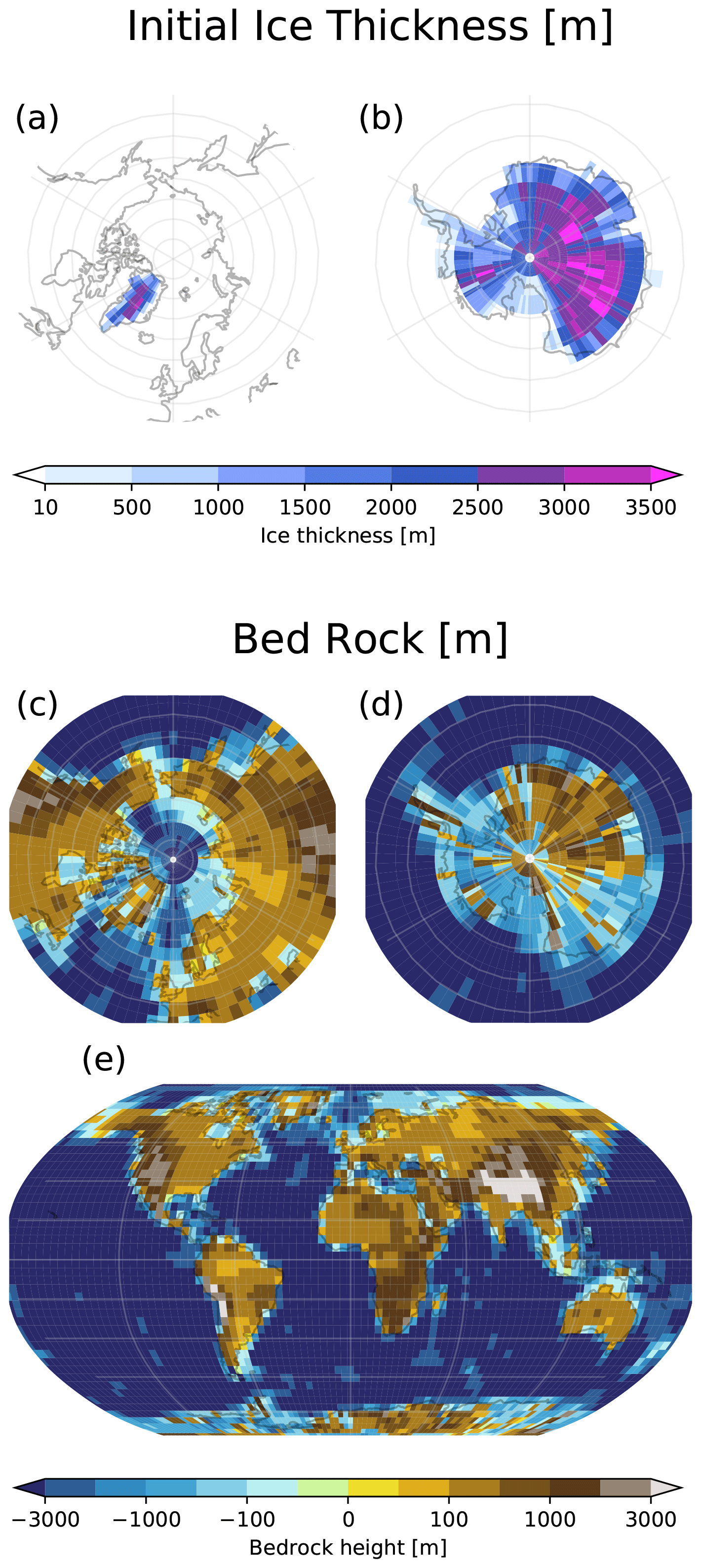
Figure 1Initial ice thickness (a, b) and bed rock (c–e) in GREB-ISM. Ice thickness less than 10 m is not shown.
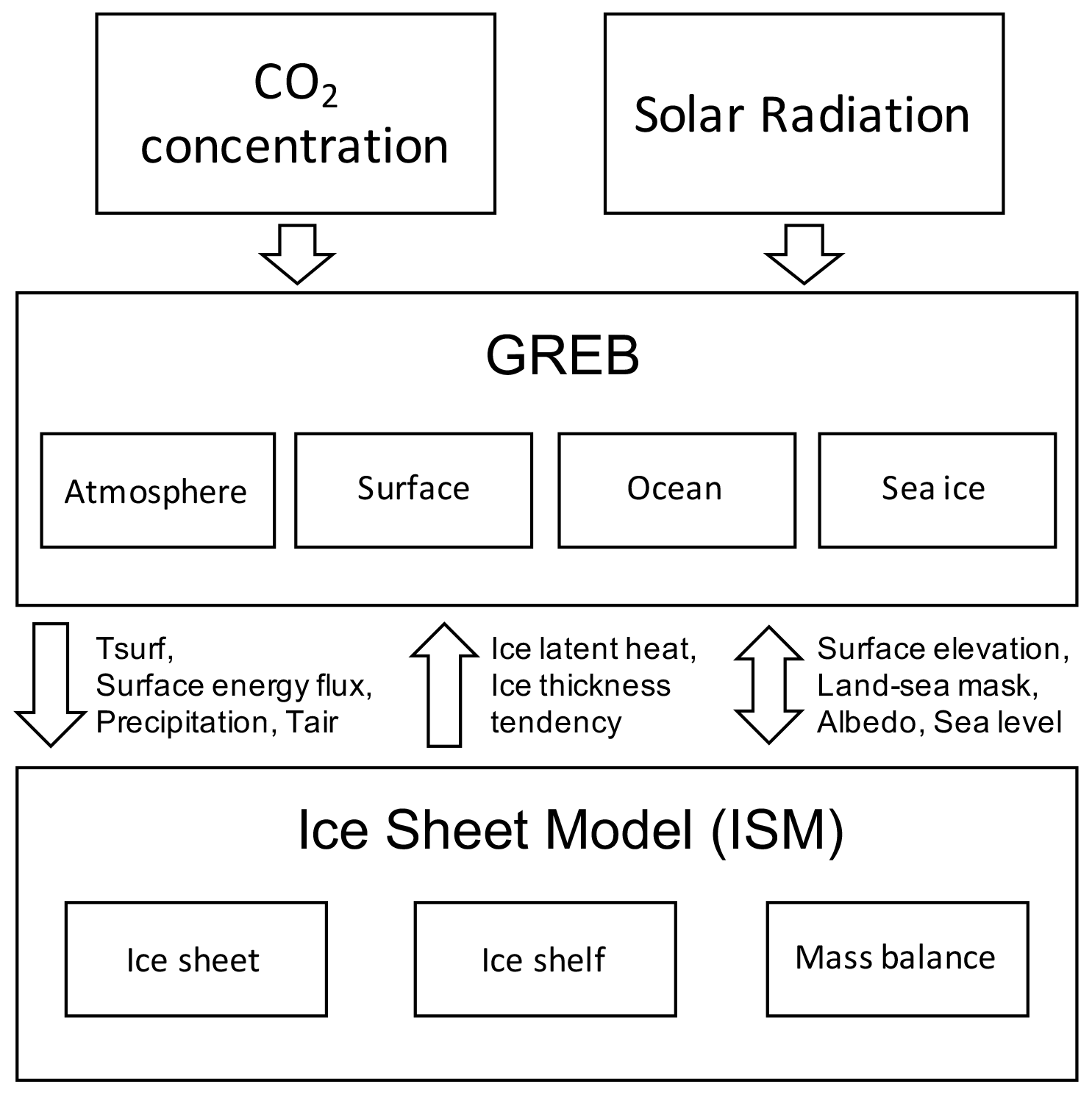
Before we introduce the ice sheet model developed in this study, we give a short description of the GREB model. We discuss changes made to the GREB model to couple the climate variables of the GREB model to the ice sheet variables, introducing the new model: GREB-ISM. All variables of the GREB-ISM model, as discussed in this study, are listed in Table 1. A model schematic of the coupling between the ice sheet and the climate model is illustrated in Fig. 2.
3.1 The Globally Resolved Energy Balance (GREB) model
The GREB model is developed and fully described in Dommenget and Flöter (2011), with the additional introduction of a new hydrological cycle model in Stassen et al. (2019). The model has three layers (atmosphere, surface and sub-surface ocean) with a global, horizontal grid spacing of 3.75∘ × 3.75∘ (96 point × 48 point). The GREB model simulates four prognostic variables: surface (Tsurf), atmospheric (Tatmos) and subsurface ocean temperature (Tocean), and surface humidity (qair):
The main physical processes that control the surface temperature tendencies are solar (short-wave) and thermal (long-wave) radiation, the hydrological cycle (including evaporation, moisture transport and precipitation), horizontal transport of heat, and heat uptake in the subsurface ocean. GREB further simulates a number of diagnostic variables, such as precipitation snow/ice cover and sea ice, resulting from the simulation of the prognostic variables.
Atmospheric circulation (mean winds) and cloud cover are seasonally prescribed boundary conditions, and prescribed flux corrections (Fcorrect, and Δqcorrect) are used to keep the GREB model close to the observed mean climate. State-independent flux corrections of surface temperatures or other variables allow a climate model to be close to those observed or any other state, while still being able to fully respond to external forcing or internal variability (Dommenget and Rezny, 2018; Irvine et al., 2013; Schneider, 1996). The flux correction terms are estimated by balancing the tendency in Eqs. (1)–(4) for observed boundary conditions to result in the observed Tsurf, Tocean and qair for each calendar month (see Dommenget and Flöter, 2011, for details).
Since the GREB model does not simulate the atmospheric or ocean circulation, it is conceptually very different from coupled general circulation model (CGCM) simulations. The model does simulate important climate feedbacks such as the water vapor and ice–albedo feedback, but an important limitation of the GREB model is that the response to external forcing or model parameter perturbations does not involve circulation or cloud feedbacks. GREB does not have any internal (natural) variability since daily weather systems are not simulated. Subsequently, the control climate or response to external forcing can be estimated from one single year, assuming an equilibrium has been reached. The primary advantage of the GREB model in the context of this study is its simplicity, speed and low computational cost. The simulation of 1 year of global climate with the GREB model can be done in about 1 s (about 100 000 simulated years per day on a desktop computer), and model simplicity allows the user to straightforwardly investigate cause and effect in coupled simulations.
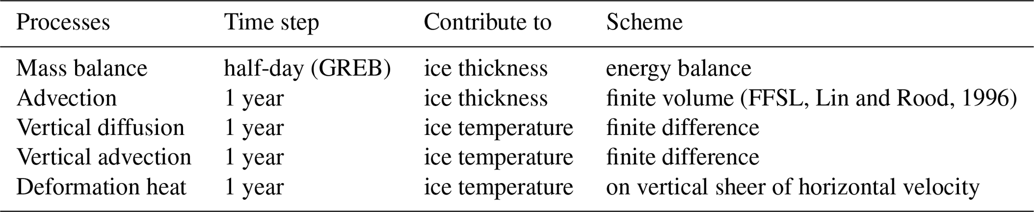
Table 2Processes and their relevant numeric scheme for the ice sheet model.
3.2 Ice sheet model
The ice sheet model is a global thermomechanical ice flow model that comprises momentum balance, mass balance and energy balance modules with the prognostic variables: thickness and temperature, and diagnostic velocities. This subsection will describe the ice sheet model, including the model grid, dynamical methods used, parameterizations and approximations made. A short summary of the basic numerical schemes used are listed in Table 2.
3.2.1 Model grid
The ice sheet model uses the same horizontal grid as the GREB model. The Arakawa C scheme (Pollard and Deconto, 2012) is adopted for the simulation of velocities, with the ice thickness and temperature specified at the center of the grid, and zonal and meridional velocities are specified at the grid boundary midpoint. For the vertical coordinates, we apply a terrain-following coordinate, ξ, in the ice sheet model, where
We chose the number of layers to be 4, to be close to the minimal number of layers which can still resolve the vertical velocity in the ice sheets: the surface layer (ξ=1), two Gaussian nodes (, nodes for 2-point Gaussian quadrature; Hildebrand, 1987) and the base layer (). The vertical integration in the model is based on Gauss–Jacobi quadrature (Hildebrand, 1987), where temperature vertical distribution is estimated by a polynomial curve fitting according to the four layers, which is expressed by
where T is the temperature, ci () are regression coefficients derived from the temperatures at the above four vertical nodes at each time step. The global, horizontal model grid has cyclic boundary conditions. For the grid points at the poles, we assume the poleward neighbor is the point at the same latitude, but shifted by 180∘, following the approach in Allen et al. (1991). To avoid numerical instability in the polar regions, a zonal wave filter is applied from 76.875∘ S to the South Pole (Lin and Rood, 1997; Suarez and Takacs, 1995).
3.2.2 Glacier mask
The GREB-ISM ice sheet evolution depends on whether the ice is grounded (land), floating (ice shelves) or if we have thin ice over the ocean (sea ice). The ice thickness, H, is used for both sea ice and ice sheet. For very thin ice cover, the gravity-driven ice flow is negligible and thus it does not follow ice sheet dynamics (e.g., snow or sea ice). To distinguish large ice mass from snow or sea ice, H must be above 10 m (Fyke et al., 2011). In detail, the points are as follows:
-
Grounded ice (land) points. Ice sheet is grounded on bedrock, satisfying the condition (Larour et al., 2012):
-
Floating ice (ice shelves) points. Ice thickness H ≥ 10 m and does not reach the bedrock, satisfying the floating condition:
-
Ocean points (all other points).. The ocean points here include sea ice grid (H≥0) as well.
The definition of this glacier mask does implicitly define groundling lines of glaciers by shifting points from grounded ice to floating ice according to the ice thickness, bed topography and global sea level (see also Sect. 3.3.8 for the sea level impact on the bed elevation).
3.2.3 Mass balance
The ice surface elevation, calculated from the mass balance equation, is the primary input from the ice sheet model to the GREB model, calculated for all global grid points. The mass balance equation is as follows:
where the accumulation of snow (s), ablation (melting) of ice (a) and ice transport ((∇⋅(VmH)) control the mass balance. The surface mass balance terms (s,a) are calculated at the same time step as GREB (half-day), and thus we have seasonal ice thickness change. The ice transport term is calculated with an annual time step (Sect. 3.2.4).
The methods used to calculate the terms on the right hand side depend on whether ice is grounded (ice sheet), floating (ice shelves) or sea ice. The mass balance for sea ice is described in Sect. 3.3.4. For the ice sheet and shelves, the two local surface forcing terms for the ice mass balance from Eq. (7) are the source (accumulation) and sink (ablation) terms. The accumulation is due to snowfall:
with the snowfall ratio, r:
The ice ablation rate is due to surface melting by positive surface heat flux:
with the latent heat flux for melting ice, Fice:
Here, the maximum heat flux for complete ice melting is . The surface heat flux, Fsurf, only considers the net surface heat flux beyond the freezing point:
and the estimated surface temperature without ice fusion is
where Fnet is defined as the right hand side of Eq. (1).
We currently do not explicitly include an ocean basal melting scheme in our model. On the one hand, our ice shelf viscosity is tuned to fit the current day ice shelf thickness, which partially contains basal melting effects (see Sect. 3.2.4). On the other hand, including a basal melting scheme (Martin et al., 2011) does not contribute to a significant improvement in our model simulations (see Sect. 4.3).
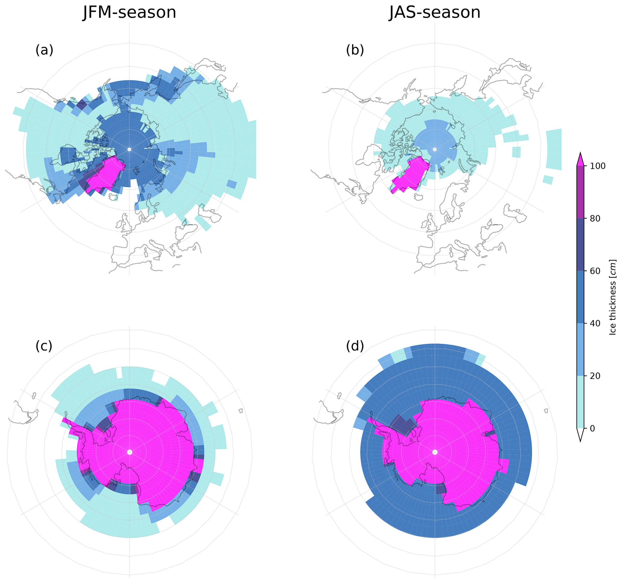
Figure 3GREB-ISM seasonal ice thickness (cm) during January–February–March (a, c) and July–August–September (b, d) from the coupled dynamic equilibrium experiment equilibrium state (200 kyr). The scale is chosen to highlight seasonal ice cover.
The snow accumulation and melting, as described above, control all land ice and snow cover and therefore also simulate the seasonal cycle of snow and ice cover over land. Figure 3 illustrates the seasonal cycle of ice cover in both hemispheres as simulated by the GREB-ISM model with present-day boundary conditions. The ice cover change for ocean points comes from sea ice changes, which is described in Sect. 3.3.4. The overall snow cover (land) distribution and seasonal cycle resemble observations (Robinson et al., 2012). Similarly, the mean sea ice extent and seasonal cycle are comparable with those observed (Rayner et al., 2003), with some overestimation of sea ice extent around Antarctica in summer.
Calving
A boundary condition for the mass transport equations is required at the ice front: here, ice from the ice sheet can be freely advected to the attached ocean grid and become sea ice (see Sect. 3.3.4 for the dynamics of sea ice). In this way, calving is diagnosed as transport from ground (land) or floating ice (shelves) onto ocean points.
3.2.4 Momentum balance
Ice flow on grounded ice points is solved based on the shallow ice approximation (SIA; Hutter, 1983; Morland, 1984) for momentum balance:
and the shallow shelf approximation (SSA; Macayeal, 1989) on floating ice points (solved in geo-coordinate latitude ϕ and longitude λ):
The viscosity (ηSSA) in our model is larger than in other models (Bueler and Brown, 2009). This high viscosity is tuned by adjusting ice shelf thickness to observation, which may be impacted by uncertainties in the observations, other model fields or in physical processes such as ice shelf basal melting effects.
Vertical velocities are recovered through incompressibility:
The deformation of ice under stress is described by Glen's flow law (Glen, 1953, 1954, 1955):
where T′ is the temperature corrected for the dependence of melting point on pressure:
In our model, the viscosity ηSSA (Table 1) has been set as a constant value to match with the observed ice surface velocity and calving in the stand-alone dynamic equilibrium experiment (Sect. 4.3). Each of Eqs. (14)–(18) above are expressed in z coordinates but are transformed into ξ coordinates for the model integration. Boundary conditions for the mechanical model are required at the ice sheet surface, base and at the ice shelf-ocean front. A stress-free ice surface is assumed:
where n is the normal unit vector at the ice surface.
At the base, the horizontal ice velocities follow the viscous-type sliding law defined in Greve (1997):
The value for Csl is as in Greve (1997). In Sect. 4.3 we discuss to what extent variations in Csl could improve the simulations.
The stress conditions for the horizontal ice shelf velocities at the interface with the open-ocean points follow Greve and Blatter (2009), which in our model is expressed as follows:
3.2.5 Energy balance
The ice temperature (energy) balance is calculated as follows:
The ice temperature balance at the surface is constrained by Tsurf as computed in the GREB-ISM model (see Sect. 3.3.1):
The geothermal heat flux is an important boundary condition for ice sheets. Previous studies show that the model with uniform geothermal heat flux is still able to reproduce the ice sheet evolution in the paleoclimate (Abe-Ouchi et al., 2007; Tigchelaar et al., 2019). For consistency, we therefore assume a globally constant bottom layer geothermal flux as in Huybrechts et al. (1996) and Payne et al. (2000):
3.3 Coupling of the GREB model to the ice sheet
The introduction of an ice sheet model requires a number of changes to the original GREB model. In the following, we describe the changes made to the GREB model equations and illustrate how they affect the simulation of the GREB climate.
3.3.1 Energy exchange between GREB and ice sheet/sea ice
The introduction of a prognostic ice sheet model introduces the additional heat flux term, Fice, for the Tsurf tendency Eq. (1), resulting in the new equation:
The calculations of Fice are described in Sect. 3.2.3 (mass balance) and Sect. 3.3.4 (sea ice). The effect of Fice can best be illustrated by a simple response experiment in which we add a 10 m ice cover and evaluate how surface temperature responds to it (Fig. 4). In this response experiment 10 m of ice cover is introduced over a large region of Europe (Fig. 4d, black box) at the start of the simulation, and then the fully coupled GREB-ISM model is run for 4 years to respond to this change.
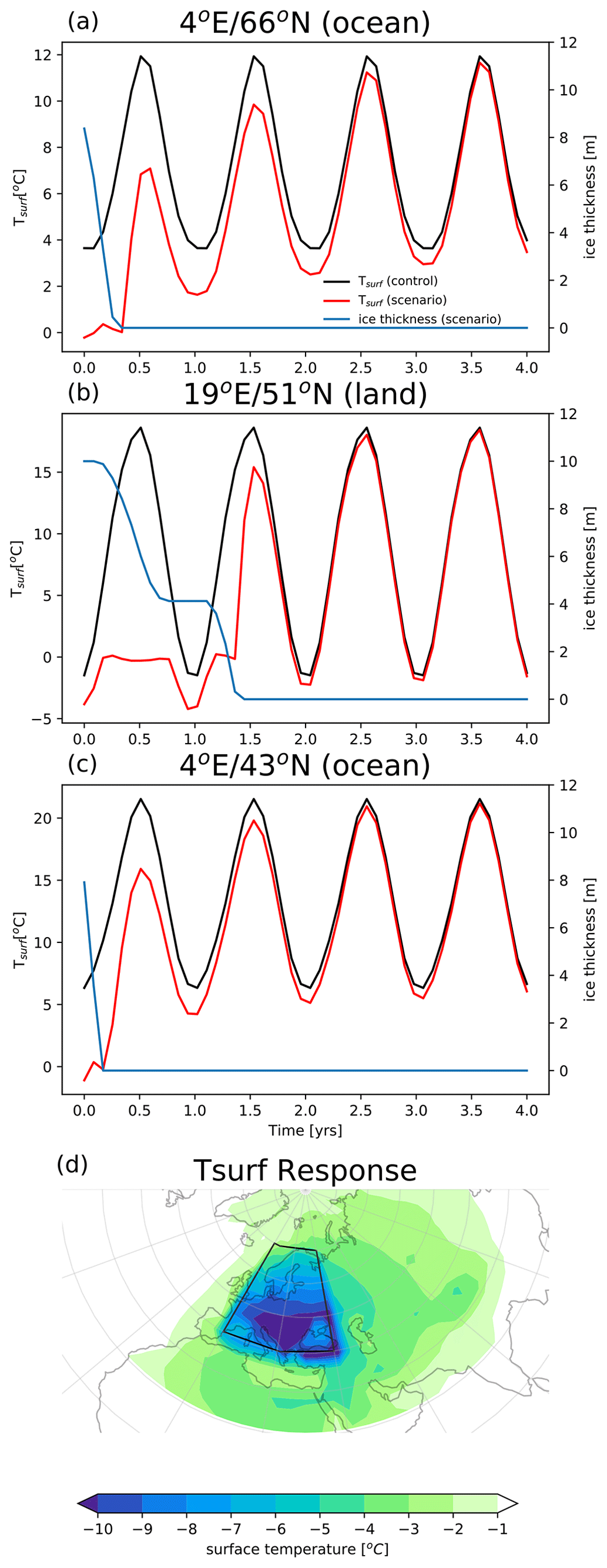
Figure 4GREB-ISM response to adding a 10 m ice sheet in surface temperature (units: ∘C) and ice thickness (units: m). In (a)–(c) are the temperature and ice thickness evolution at three different locations. The black, red and blue curve represent control run surface temperature (without adding 10 m ice), scenario run surface temperature (with adding 10 m ice) and scenario run ice thickness. Panel (d) shows the temperature difference (units: ∘C) between scenario and control at the end of the first simulation year. The black outlined region in (d) mark the area in which the initial 10 m ice sheet is added.
The introduction of the ice cover forces surface temperature below the freezing point at all locations, as long as the ice sheet is present (Fig. 4a–c). The atmospheric heat fluxes and sea ice dynamics force the sea ice to melt, which it does faster over the ocean points due to horizontal sea ice transport. Over land the ice cover melts after the first year and allows surface temperature to go back to the control run values. The atmospheric heat and moisture transport cause cooling in adjacent regions (Fig. 4d).
3.3.2 Surface heat capacity
The surface layer effective heat capacity (γsurf) in the GREB model is equal to the heat capacity of a water column of the mixed layer depth over ice-free ocean points and equivalent to 2 m soil for all other points (e.g., land and ice covered). Thus, the formation of sea ice changes the heat capacity from that of the mixed layer depth to a 2 m soil column. This is unchanged from the original GREB model.
3.3.3 Precipitation correction
The hydrological cycle model in GREB developed in Stassen et al. (2019) simulates precipitation as a function of the simulated atmospheric humidity (qair), the observed mean and standard deviation of the vertical air motion (ωmean, ωSD):
This model aimed at a realistic simulation of precipitation with a focus on the regions of greatest precipitation, i.e., the tropical oceans. While the precipitation model is very good in these regions (Stassen et al., 2019), it only has limited skills over higher-latitude land regions, which are most important for the ice sheet mass balance of the GREB-ISM.
To allow the ice sheet mass balance to receive unbiased mean precipitation forcing under present-day conditions, we introduced a land precipitation correction in the GREB-ISM model. The new precipitation equation with flux correction is expressed as follows:
where qzonal⋅pcorrect is the flux correction of the equation. The flux corrections are only active over land and are a function of calendar month. They are estimated in a way that the simulated Δqprecip matches the precipitation data in Sect. 2 for every calendar month of the year.
Here, we note that the model assumes that precipitation is proportional to the local humidity (qair). Stassen et al. (2019) demonstrate that this assumption is less appropriate in higher-latitude land regions, as there is no clear relationship between the local qair and Δqprecip. Due to the lack of a clear local relationship, we relaxed this constraint and assumed that the precipitation over land is a function of the zonal mean humidity, reflecting the mostly zonal structure of the atmospheric circulation. Therefore we set the correction term to be proportional to the zonal mean qair defining qzonal. Within 30∘ of the poles qzonal is estimated as the mean from the pole to 60∘.
With this approach the precipitation over higher-latitude land responds to cooling or warming similarly to other regions (e.g., oceans for lower latitudes). We will discuss the precipitation response of the GREB-ISM further below in the context of the response experiments.
3.3.4 Sea ice
Sea ice is a diagnostic variable in the original GREB model but is now changed to be a prognostic variable in GREB-ISM. Over land and ice shelf points, ice thicknesses (H) follow the dynamics described in the ice sheet model Sect. 3.2. Over ocean points we use the same prognostic variable (H), but the sea ice thickness dynamics follow a different tendency equation, namely
with the local sea ice growth,
and where the latent heat of ice fusion Fsurf is defined by Eqs. (11)–(13):
The sea ice growth threshold of 0.5 m reflects the fact that sea ice is a very good insulator and subsequently does not transfer atmospheric heat fluxes very well once a certain ice thickness is reached. This in practice limits the growth of sea ice by atmospheric heat flux to less than 0.5 m typically. In this case Fice=0 and it will no longer grow the sea ice, but only cool Tsurf (Eq. 28).
Sea ice transport is estimated by isotropic diffusion (κsi∇2H). This approximates the effect of turbulent winds and ocean currents transporting sea ice, leading to fast decay of sea ice near open ocean. The diffusion coefficient κsi was chosen to roughly lead to a sea-ice-decaying timescale of about 1 month.
3.3.5 Albedo coupled to ice sheet
The surface albedo (αsurf) in the original GREB model was diagnosed as function of Tsurf but is now diagnosed as a function of the ice thickness (H):
The linear relation between ice thickness and albedo in the GREB-ISM model was estimated from the assumption that for the observed northern hemispheric seasonal cycle of snow/ice cover over land the overall albedo matches the mean overall albedo of the original GREB model.
3.3.6 Topography coupled to ice sheet
The land topography (ztopo) in the original GREB model is a fixed boundary condition that influences a number of processes: thermal radiation, hydrological cycle, and the transport of heat and moisture by advection and diffusion. For GREB-ISM the land topography is now a function of the bed topography and ice sheet height:
The GREB-ISM does not simulate any glacial isostatic adjustment.
3.3.7 Sensible heat flux between surface and atmosphere
The variable land topography (ztopo) should affect the sensible heat flux between Tsurf and Tatmos, which was not simulated in the original GREB model. Here it needs to be considered that the GREB model does not resolve the vertical structure of the atmosphere, as it only has one atmospheric layer. However, in the real world Tatmos decreases with surface elevation, following a moist adiabatic lapse rate. We therefore change the sensible heat flux between Tsurf and Tatmos, which was approximated in the original GREB model by Newtonian coupling between Tsurf and Tatmos. In the GREB-ISM model this is now replaced with a Newtonian coupling between Tsurf and an adjusted Tatmos:
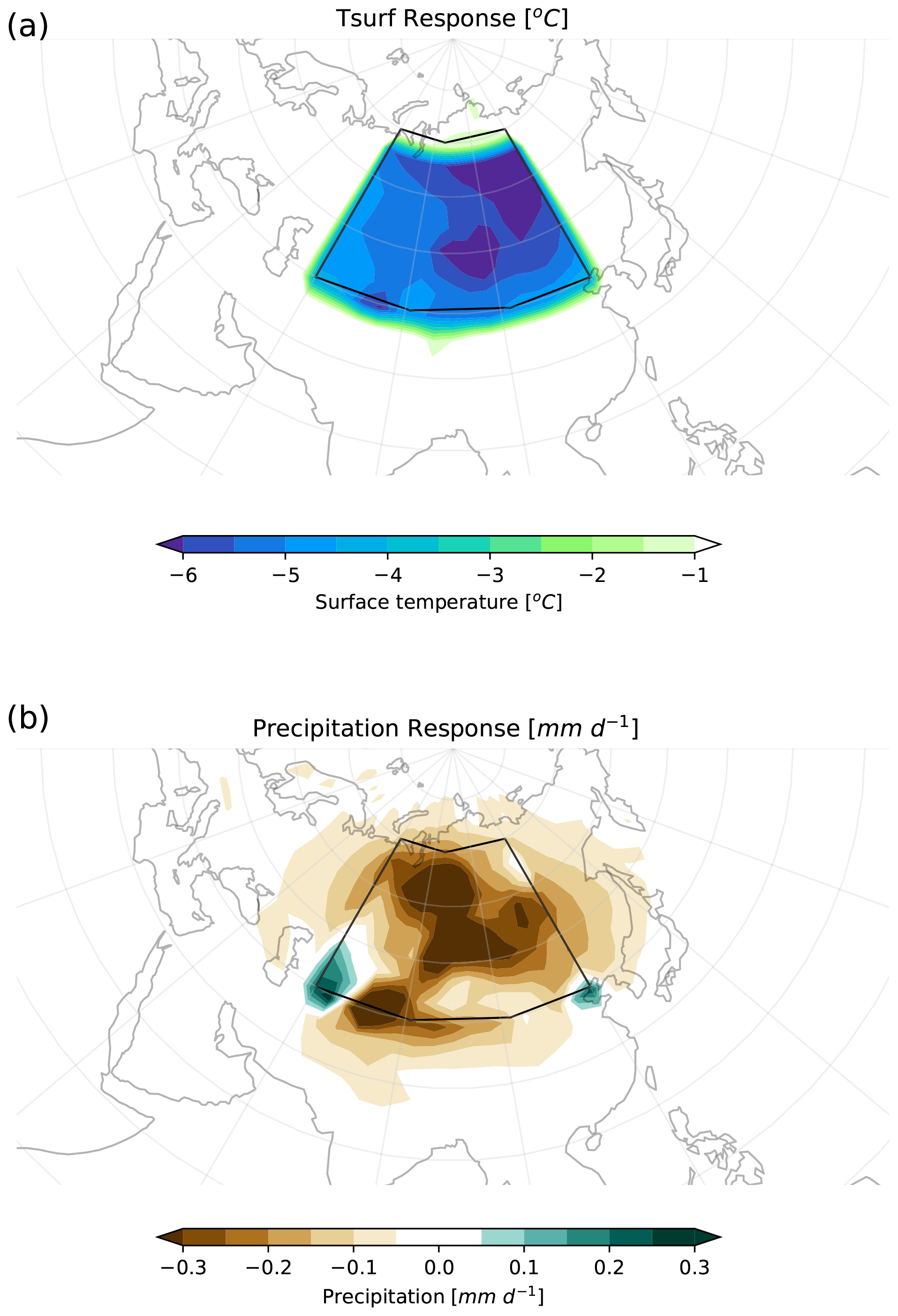
Figure 5GREB-ISM response to a lifting of the topography by 1000 m for surface temperature (a, units: ∘C) and precipitation (b, units: mm d−1). The response is defined as the scenario run (1000 m topography lifting) minus control run (no lifting) at the end of the first simulation year. The box represents the lifted region.
Here we choose a globally constant moist adiabatic lapse rate Γ = −6 K km−1. The effect of this sensible heat flux is illustrated with a simple response experiment; see Fig. 5. For this experiment we increase ztopo and precipitation relative to a control simulation with no changes in ztopo (Fig. 5). Tsurf decreases in response to the topographic perturbation, approximately linearly to the moist adiabatic lapse rate. The higher topography also affects the hydrological cycle, reducing the precipitation locally and also remotely through transport of relatively reduced atmospheric humidity.
3.3.8 Sea level and land–sea mask
A sea level subroutine is added in GREB-ISM. Only grounded ice thickness impacts the global sea level. Consequently, the sea level change slv is defined by
where Href is the reference ice thickness, Aocean is total area of ocean grid and ∫groundeddA is an integration over all grounded ice points. slv will be added to bed topography b, which eventually impacts the land–sea mask. The sea level and land–sea mask are updated every model year.
The soil moisture, which is a boundary condition for estimating surface evaporation, is initially set to observed values over land and then changes if land–sea distribution alters. If the sea level lowers and an ocean point turns into a land point (b > 0) then the land point has a soil moisture value of 0.3 (equivalent to the mean value for land points in Dommenget and Flöter, 2011). In turn, if the sea level rises and a land point turns into an ocean point (b < 0), then the soil moisture value is set to 1.0.
3.3.9 Meridional heat transport
The study by Dommenget et al. (2019) showed that the GREB model, without flux corrections for Tsurf, has a high-latitude climate that is too cold and a tropical climate that is too warm, indicating that the meridional heat transport is too weak. The meridional heat transport in the GREB model results from the atmospheric heat transport by the mean advection due to the mean horizontal wind field and by isotropic diffusion. The latter depends on the diffusion coefficient in the GREB model. This value is not strongly constrained by observations and may effectively be different by an order of magnitude. Since the meridional heat transport may play an important role in the global ice-age cycle, we enhance this diffusion coefficient by a factor of 5. This reduces the mean Tsurf bias in higher latitudes and the tropics in the GREB model without flux corrections, while at the same time does not increase biases in other locations, indicating it is a better approximation of the isotropic diffusion.
We start our evaluation of the new ice sheet model GREB-ISM with stand-alone ice sheet model simulations forced with idealized or observed boundary conditions. These simulations focus on the ice sheet simulation only. Section 4.1 and 4.2 use standard experiments from the European Ice Sheet Modelling Initiative (EISMINT) model intercomparison Phase I (Huybrechts et al., 1996) and II (Payne et al., 2000), which test the ice sheet model response to idealized mass and temperature forcing within a given horizontal resolution, with the ice mechanics decoupled from the thermodynamics in EISMINT I and coupled in EISMINT II. In Sect. 4.3, we discuss a simulation on the global GREB-ISM grid forced with observed boundary conditions to estimate the dynamically forced equilibrium of the ice sheet model. Finally, we discuss an idealized time-varying ice sheet response experiment, forced with temperature and precipitation similar to (Niu et al., 2019) over the past 250 kyr.
Table 3Variables (upper) and parameters (below) list for EISMINT experiments.
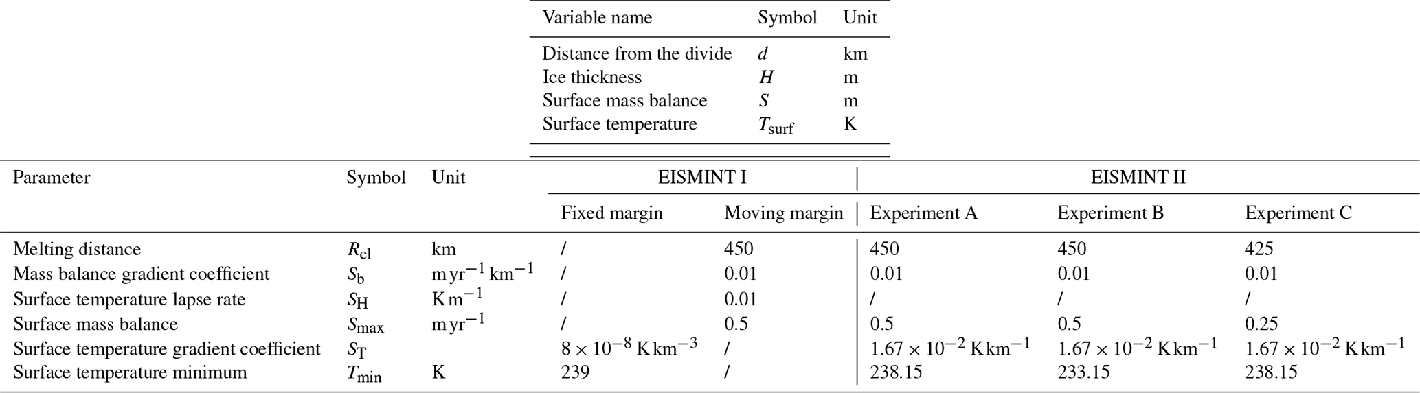
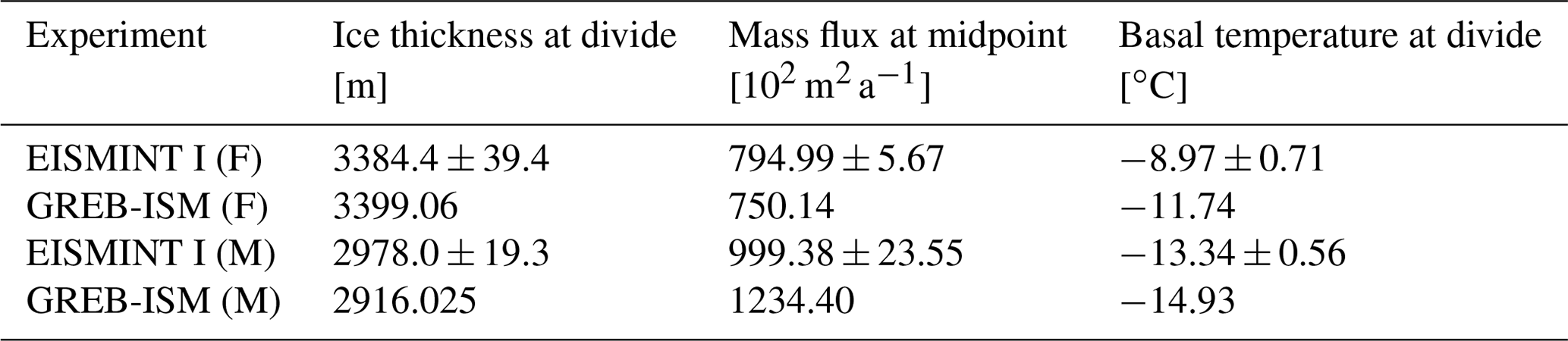
Table 4EISMINT I steady state experiment result comparison between GREB-ISM and the model ensemble from H96 for fixed-margin (F) and moving-margin (M) experiments.
4.1 EISMINT I
All simulations in EISMINT I (Huybrechts et al., 1996, H96 hereafter) are based on a regional grid in Cartesian coordinates that have higher resolutions than the GREB model grid (∼ 50 km). For a better comparison of the numerical schemes we changed the GREB-ISM grid (3.75∘ × 3.75∘) for these experiments to a model grid with 96 points in the zonal and 144 points in the meridional direction (3.75∘ × 1.25∘). Only the first 15 points in the meridional direction are used for the ice sheet simulation. The ice sheet divide in these simulations is the South Pole, and the length of the meridional grid is 50 km. The simulations are integrated for 200 kyr, but near equilibrium is reached after about 50 kyr.
The mass balance S and surface temperature Tsurf forcings are given as follows:
The parameters in Eqs. (38) and (39) are listed in Table 3. Table 4 shows the comparison between the new ice sheet model GREB-ISM and model results from H96. The GREB-ISM simulations of the ice thickness at divide and mass flux at midpoint are mostly similar to those found in H96 for both the fixed and moving margin experiments. The ice mass flux in the GREB-ISM is larger than in H96 for the moving margin experiment. An additional experiment (not shown) with the GREB-ISM in Cartesian coordinates as used in the EISMINT I simulation finds the ice mass flux close to H96, suggesting this result may be dependent on mesh shape.
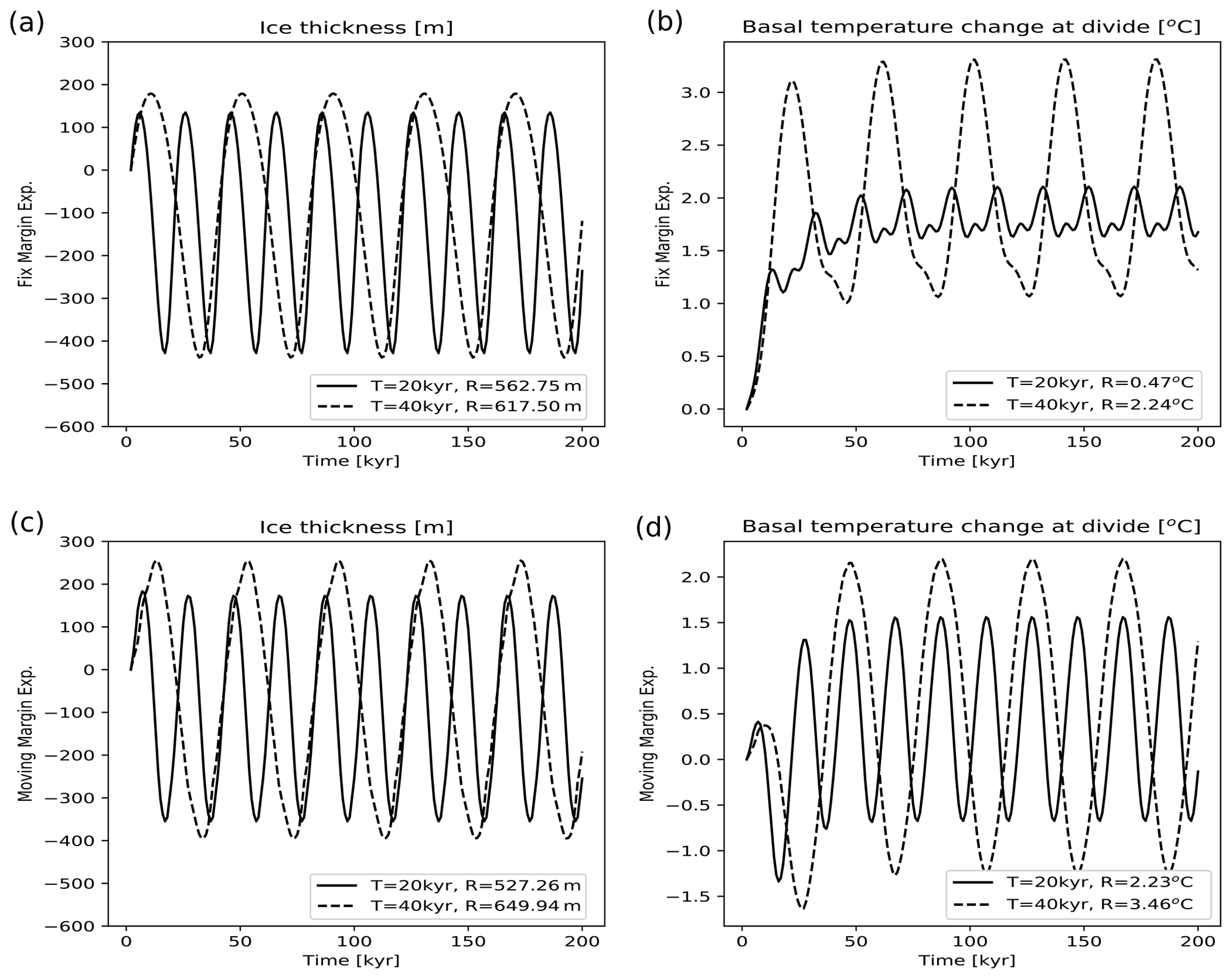
Figure 6Time evolution of ice thickness (a, c, unit: m) and homologous basal temperature (b, d, unit: K) in the EISMINT I fixed (a, b) and moving (c, d) margin experiments with GREB-ISM with 20 and 40 kyr period forcing. R marks the range (maximum minus minimum in the last 50 kyr) of the simulated variables.
The transition experiments with oscillating forcing of temperature and mass balance with periods of 20 and 40 kyr are presented in Fig. 6. The GREB-ISM ice thickness simulation is similar to those of H96 for both fixed and moving margin experiments (Fig. 6). In both experiments, the basal temperature at the divide is about 1–2 ∘C colder than in the H96 simulations, which is related to the coarse vertical resolution. This mismatch disappears if we increase the vertical resolution to 10 layers (not shown).
Table 5Results for basic glaciological quantities in EISMINT II experiments after 200 kyr. Differences are defined as current experiment minus experiment A. Percentage changes are relative to experiment A. The results of P2000 are shown in the form of “mean ± range”. See text for details.
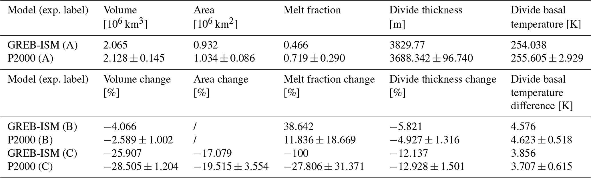
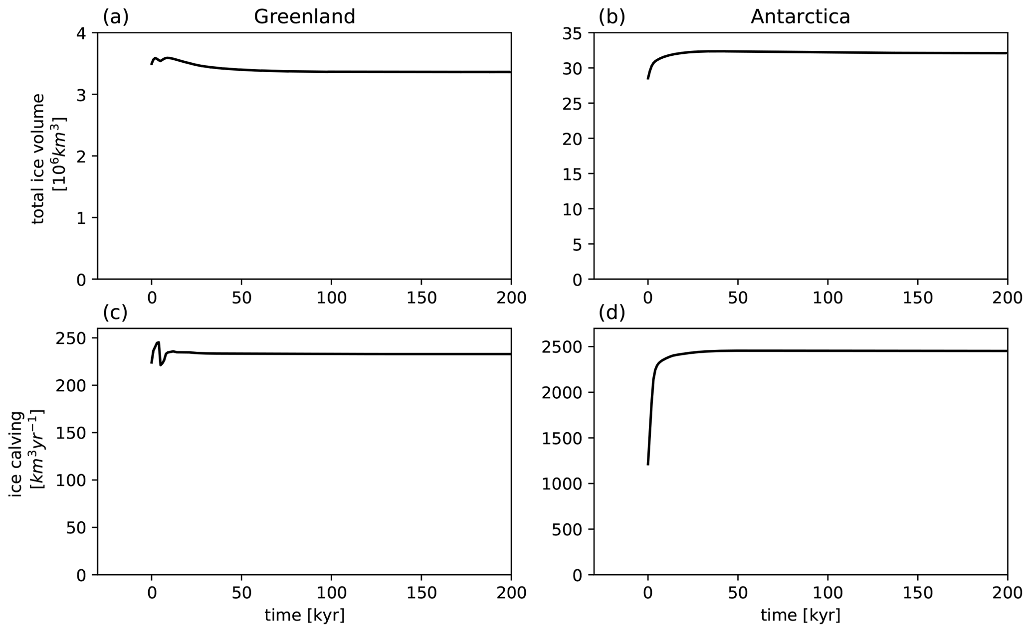
Figure 7Time evolution of total ice volume (a, b, units: 106 km3) and ice calving (c, d, units: km3 yr−1) in Greenland (a, c) and Antarctica (b, d) from the forced stand-alone dynamic equilibrium experiment.
4.2 EISMINT II
EISMINT II experiments (Payne et al., 2000, P2000 here after) involve coupling between the mechanical and thermodynamical components of the ice sheet model. These experiments are designed to test how the ice sheet temperature variations interact with the ice sheet transport. The GREB-ISM model grid used is similar to in EISMINT I, but the number of points in the meridional direction is increased from 15 to 31 and the length of the meridional grid is set to 25 km. All experiments are integrated for 200 kyr. The boundary conditions for the first experiment (A) are as follows:
with the parameters given in Table 3. The results of experiment A are summarized in Table 5. The final GREB-ISM values for ice volume, area, divide thickness and basal temperature at the ice sheet divide are all within the range of the models in P2000, indicating a fairly good agreement. The basal melt fraction is underestimated by the GREB-ISM by about 30 %, which is related to a cold bias at the bed of the ice sheet.
Experiment B and C in EISMINT II are designed for testing the model sensitivity to various boundary conditions. Tmin in experiment B is set as 5 K cooler than in experiment A, to evaluate the sensitivity of the model to the mean ice temperature. Table 5 depicts the difference between experiment B and A. The GREB-ISM shows, in general, similar changes in ice volume, ice divide thickness and ice divide basal temperature as in P2000. However, the basal melt fraction change shows a significant discrepancy, which is related to the cold bias of the basal temperature in experiment A.
For experiment C, Smax and Rel are set as 0.25 m yr−1 and 425 km, respectively, to evaluate the impact of different mass balances. The results of experiment C are shown in Table 5. For the changes in ice volume, area, divide thickness and divide basal temperature, the response difference between experiment C and A in GREB-ISM is equivalent to results from P2000. The changes in melt fraction in the GREB-ISM deviate from those of P2000, which is again likely to be related to the cold bias in basal temperatures in the GREB-ISM in experiment A.
Overall, the model reproduces the total ice thickness and ice cover well in the idealized experiments of EISMINT I and II. Although there is a bias in the basal temperature estimation in GREB-ISM, this issue does not have a significant impact on the ice thickness and cover area, which suggests the model is appropriate for global climate and ice evolution simulations.
4.3 Globally forced dynamical equilibrium
We now focus on simulating the observed global ice sheets forced with present-day boundary conditions. Although we cannot assume that observed Greenland and Antarctic Ice Sheets are in equilibrium with present-day forcing, the dynamic equilibrium simulation should produce a global ice sheet distribution similar to the current observations.
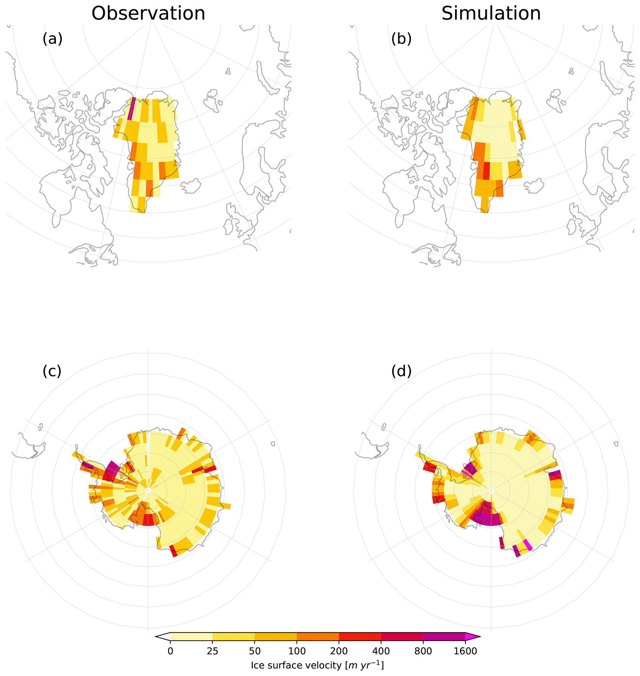
Figure 8Comparison of ice surface velocity (unit: m yr−1) from observations (left) and the GREB-ISM forced stand-alone dynamic equilibrium experiment at equilibrium state (right).
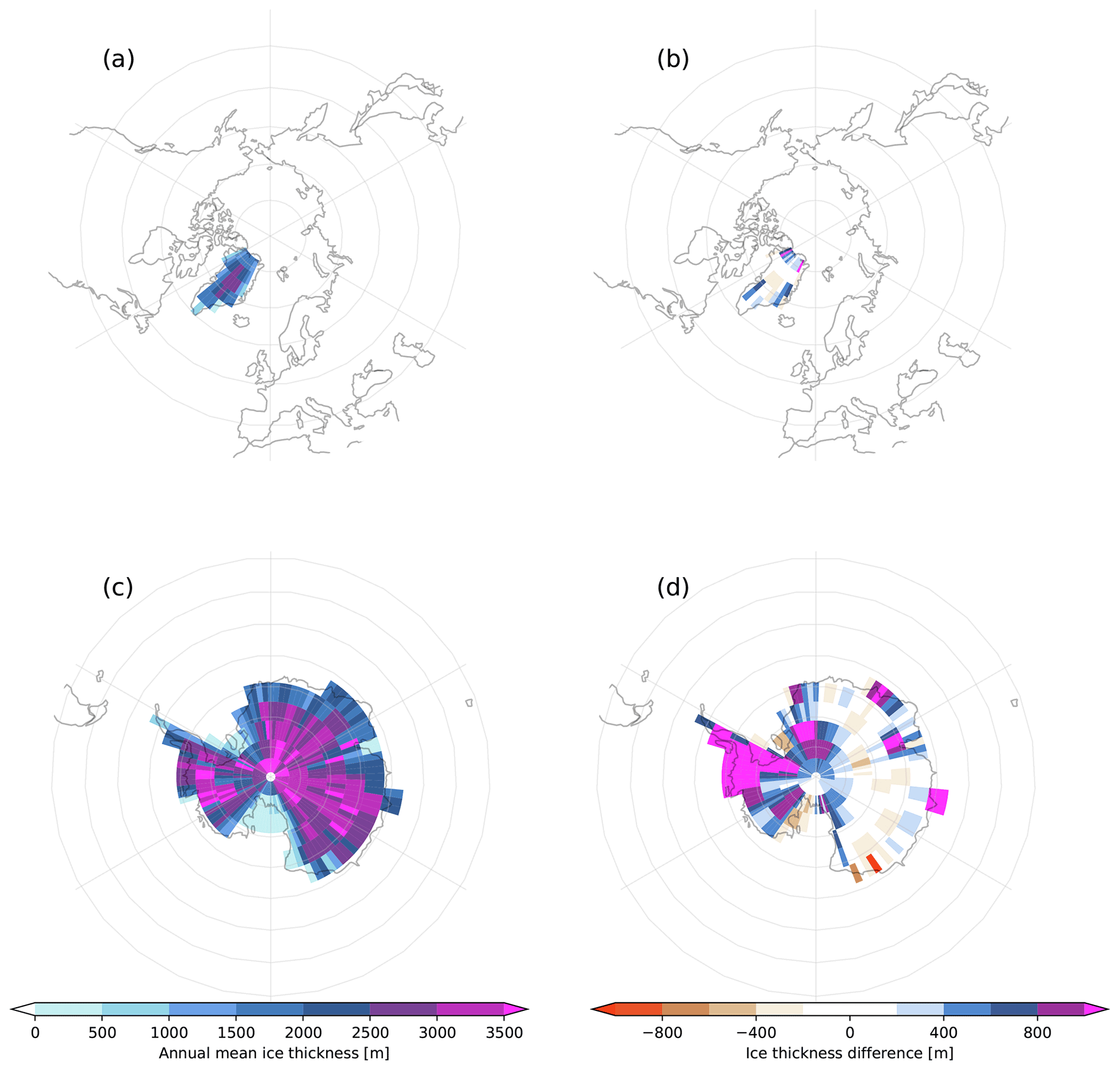
Figure 9Results from the GREB-ISM forced stand-alone dynamic equilibrium simulation at equilibrium state: annual mean ice thickness (a, c) and the ice thickness difference (b, d) between GREB-ISM simulation and the observation in Greenland (a, b) and Antarctica (c, d). The ice thickness observation is derived from the BedMachine dataset (Morlighem et al., 2017, 2020).
Table 6Ice volume and boundary calving from the forced dynamic equilibrium experiment and observation.
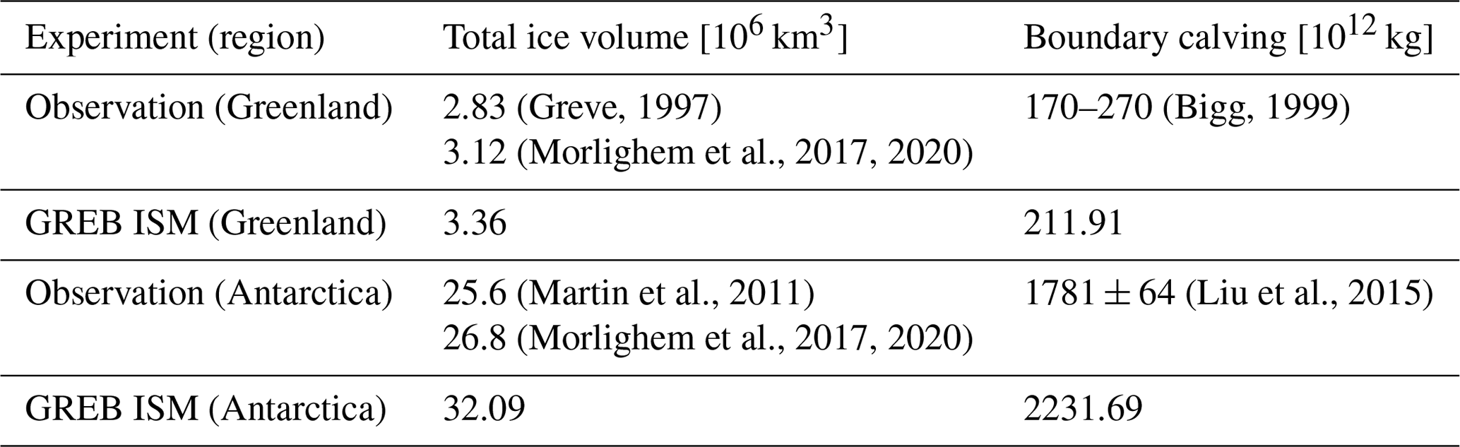
Ice surface temperature and precipitation forcings in the experiment are set to the climatologies derived from ERA-interim, NCEP-DOE and GPCP data. GREB-ISM is run for 200 kyr, initialized with observed ice thickness. Figures 7–9 show results from this simulation, and Table 6 compares the simulation values of total ice volume boundary calving with observed values from the literature.
The model reaches an equilibrium after about 50 kyr for both the Northern and Southern Hemispheres. Greenland ice thicknesses and calving rates show only small differences compared with the initial values. They are also within the estimated calving values from observation (Bigg, 1999). The trends in Antarctica are larger, in particular over West Antarctica. Here we see a significant increase in ice volume and calving (Figs. 7d and 9d). The West Antarctic ice sheet thickness increase is inconsistent with the observed values, suggesting a model limitation.
We could not find the specific limitation that is causing West Antarctic Ice Sheet bias. The precipitation forcing does play a role in controlling the West Antarctic Ice Sheet, but we could not find any reasonable precipitation forcing that would result in significantly improved simulations of the West Antarctic Ice Sheet. The parameterization of the floating ice for ice shelves (SSA) also impacts the simulation of West Antarctic Ice Sheet. The ice shelf can grow and become grounded as an ice sheet with lower viscosity. However, again we could not find any reasonable value for the ice viscosity (ηSSA) that would significantly reduce this bias. We further tested different sliding law coefficient Csl, ranging from 6 × 10³ to 6 × 10⁵ yr−1. The result indicates that the varying coefficient values do not bring a fundamental simulation improvement. Similarly, a basal melting scheme (Martin et al., 2011) with different strength has also been tested, but improvement could not be found.
The simulated ice surface velocity for Antarctica and Greenland shows a reasonable pattern, capturing the main features of the transport (Fig. 8) and the mean values. For Antarctica the ice mean flow is 109 m yr−1, faster than the observation (80 m yr−1) from MEaSUREs data (Mouginot et al., 2012; Rignot et al., 2011, 2017), and slower in the interior and faster near the boundaries. The largest velocities (more than 1000 m yr−1) appear in ice shelf regions (Ross and Filchner–Ronne Ice Shelf), which is due to the presence of the floating ice for ice shelves (SSA). Similarly, Greenland ice velocities are also in good agreement with observations (Joughin, 2017; Joughin et al., 2010) in terms of pattern and mean flow magnitude (57 simulated and 56 m yr−1 observed).
4.4 Transition experiment
We next evaluate the capability of the global ice sheet model to respond to realistic changes in the boundary conditions. We therefore design an experiment, in which we force the GREB-ISM with surface temperature and precipitation over the past 250 kyr, similar to the one discussed in Niu et al. (2019) for the Northern Hemisphere, but extended to the whole globe to evaluate the response of the ice sheet on a global scale. The surface temperature and precipitation forcing for this experiment are as follows:
The surface temperature (Tsurf) and ice mass balance (S) are present-day regional and seasonally varying climatologies (Ttoday, Stoday) plus a seasonally changing (tday) forcing pattern for Tsurf and S that varies according to δ18O proxy data derived from the Greenland Ice Core Project (GRIP) dataset (Greve, 1997). and represent δ18O at the present day and Last Glacial Maximum (LGM), respectively. The LGM reference climate forcing pattern is taken from the AWI Earth system model (AWI-ESM) (see Sect. 2 for detail), which results from a CGCM simulation forced by insolation, greenhouse gas and ice sheet. The main feature of this forcing pattern (not shown) is a much colder climate (more than 10 ∘C) from North America to Central Asia and Antarctica, which contained or were surrounded by large ice sheets (Kageyama et al., 2017). The simulation is integrated between −250 kyr and the present and initialized with present-day observed ice thickness.
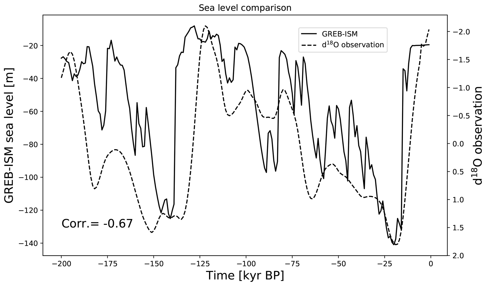
Figure 10Time series of simulated sea level (left axis; units: m) from the stand-alone transition experiment and δ18O proxy data (right axis, the axis has been inverted).
The time series in Fig. 10 depicts the sea level change in this simulation from −200 kyr BP compared with a δ18O proxy time series from ocean sediments (Imbrie et al., 1984). The two curves show similar time series variations with a correlation of −0.67. This indicates that qualitatively the GREB-ISM ice sheet shows similar overall global ice sheet variations to those observed over the past 200 kyr. The GREB-ISM sea level varies by about 120 m, which is the same as observed sea level changes (Fairbanks, 1989; Lambeck et al., 2014), indicating that the simulated ice sheet volume variations are similar to those observed. The sea level is also 20 m lower than the present day due to the excess West Antarctic Ice Sheet volume that we also observed in the dynamical equilibrium simulation.

Figure 11Global ice thickness (unit: m) distribution in the Last Interglacial (a, b), the Last Glacial Maximum (c, d) and present day (e, f) from the stand-alone transition experiment.
There are several significant extremes in the past 200 kyr simulation, which correspond to the Last Interglacial (LIG; −127 kyr), Last Glacial Maximum (LGM; −21 kyr) and the present day. The ice sheet thicknesses for these three time periods are shown in Fig. 11. During the LIG, only the Greenland Ice Sheet thickness exceeded 400 m in the Northern Hemisphere, and the Antarctic Ice Sheet thickness is similar to present day. During the LGM large European (e.g., Fennoscandia) and North American (Laurentide) ice sheets are reproduced with thousands of meters ice thickness, which is also what we expected according to previous studies (Clark et al., 2009; Velichko et al., 1997).
Table 7Annual mean ice volume in the stand-alone transition experiment for different time periods from GREB-ISM simulation and from Fyke et al. (2011).
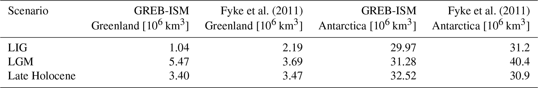
The estimate of ice sheet volume in Greenland and Antarctica for the Last Interglacial, Last Glacial Maximum and Late Holocene from GREB-ISM and from Fyke et al. (2011) are presented in Table 7. Overall, our simulation of the Greenland Ice Sheet is similar to Fyke et al. (2011) but with larger time variations. However, the simulation of Antarctica ice thickness shows very little to no variation between these three periods. The difference between the GREB-ISM model and Fyke et al. (2011) in Antarctica ice sheet may be due to different experimental setups. Fyke et al. (2011) varied and changed the ice shelf parameterization periods during their simulation, which was not done in our experiments. In summary, the results of this experiment indicate that the GREB-ISM ice sheet model does have realistic responses to time-varying boundary conditions.
We now focus on the fully coupled GREB-ISM model, in which the ice sheet and other climate variables are interacting in both directions. In the following sections, two sets of experiments are presented. First a dynamic equilibrium experiment is conducted, which is similar to the experiment discussed in Sect. 4.3, but now fully coupled with fixed boundary conditions. Second, a set of experiments with shortwave radiation oscillating on periods of 20, 50 and 100 kyr for the Northern Hemisphere are conducted. Those two experiments are designed to evaluate how coupling influences the model's behavior and to what extent the ice sheet responds to periodic solar forcing. The discussion of these experiments will focus on the introduction of the GREB-ISM model. A more detailed analysis of the ice sheet dynamics coupled with climate dynamics is left for future studies.
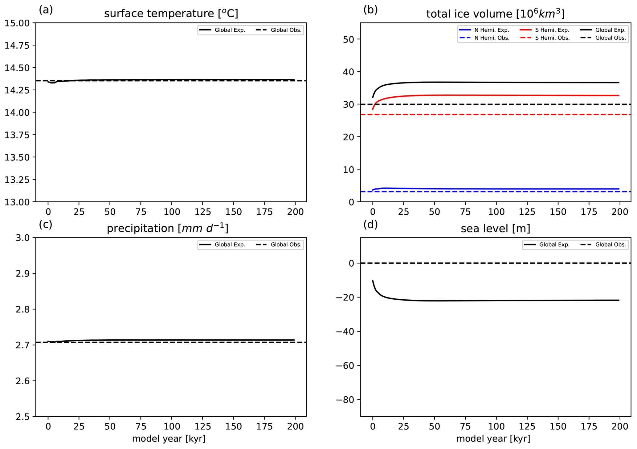
Figure 12Results from the fully coupled dynamic equilibrium experiment: evolution of global annual mean surface temperature (a, units: ∘C), total ice volume (b, units: 106 km3), annual mean precipitation (c, units: mm d−1) and sea level change (d, units: m). The dashed lines are modern observation references.

Figure 13Same as Fig. 9 but for the coupled dynamic equilibrium experiment.
5.1 Dynamic equilibrium for present-day conditions
In this experiment, the GREB-ISM model is fully coupled and forced with the fixed boundary conditions of present-day 340 ppm CO2 concentration and solar radiation. Tsurf and land precipitation are flux-corrected to the mean present-day values. However, those flux-corrected variables can respond to changes in the climate system, since the flux correction terms are state-independent (see Sect. 3.1). The simulation is 200 kyr long and results are shown in Figs. 12 and 13.
Tsurf and precipitation show no long-term drift and are close to the observation (Fig. 12a and c). Both reach equilibrium after about 50 kyr. The global ice volume difference is mainly contributed by ice thickness difference in the Southern Hemisphere (Fig. 12b), which is similar to the one in the forced experiment discussed in Sect. 4.3 (Figs. 7 and 9). As the ice volume increases, the sea level shows a clear decrease tendency and reaches equilibrium after 50 kyr as well. The ice thickness spatial pattern in the coupled experiment is comparable to the stand-alone experiment (Figs. 13 and 9). Overall, this control run simulation shows that the coupled GREB-ISM system converges towards an equilibrium state close to the observed one. The simulated trends appear to be mostly due to the anomalous growth of the West Antarctic Ice Sheet.
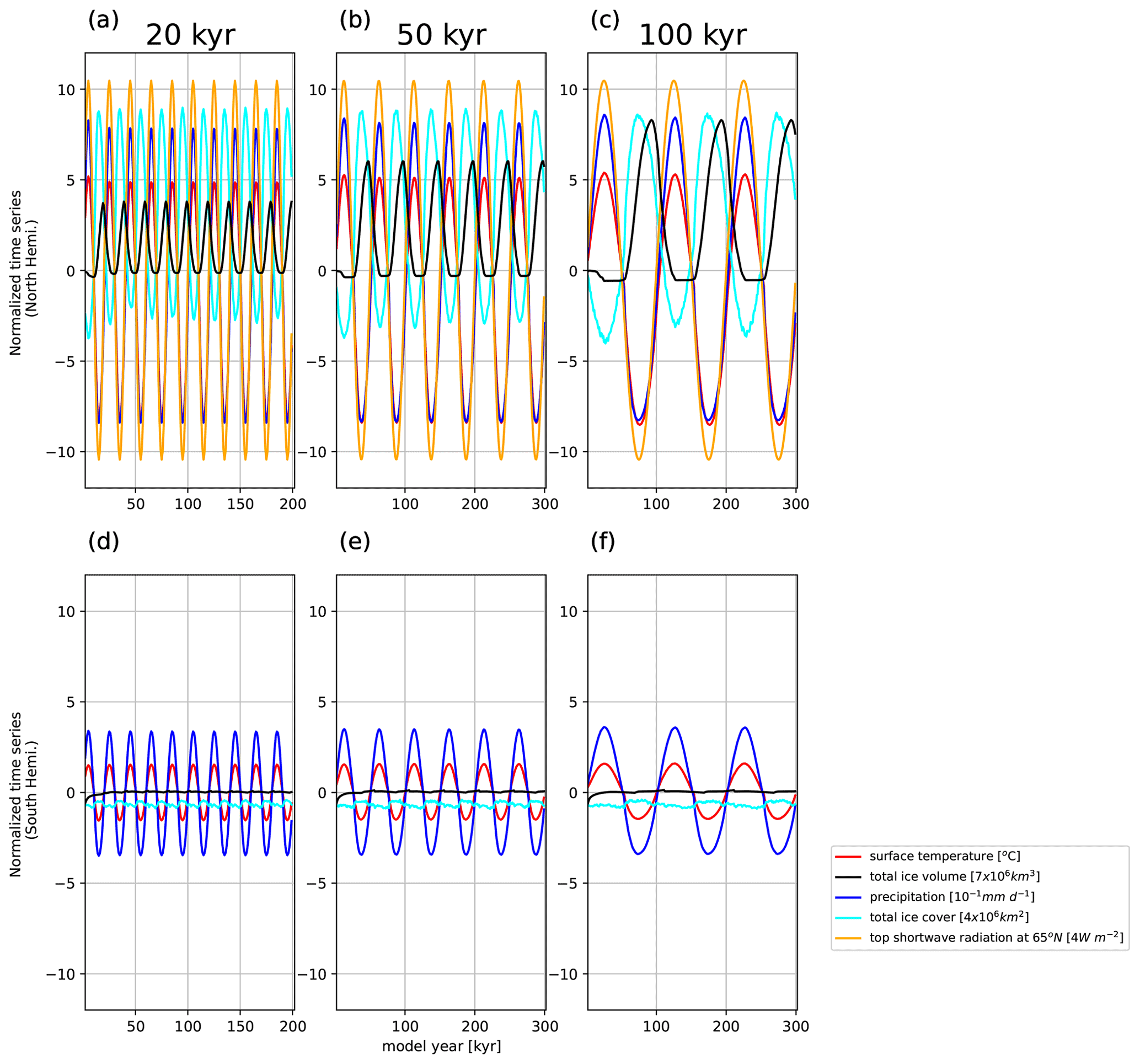
Figure 14Time evolution of change in total ice volume (black, unit: 7 × 10⁶ km3), surface temperature (red, unit: ∘C), precipitation (blue, unit: 10−1 mm d−1), ice cover area (cyan, unit: 4 × 10⁶ km2) and solar radiation at 65∘ N (orange, unit: 4 W m−2) from the shortwave oscillation experiment in Northern (upper) and Southern (lower) Hemisphere with forcing period of 20 kyr (a, d), 50 kyr (b, e) and 100 kyr (c, f). The control equilibrium state values from the coupled dynamic equilibrium experiment are removed to obtain changes.
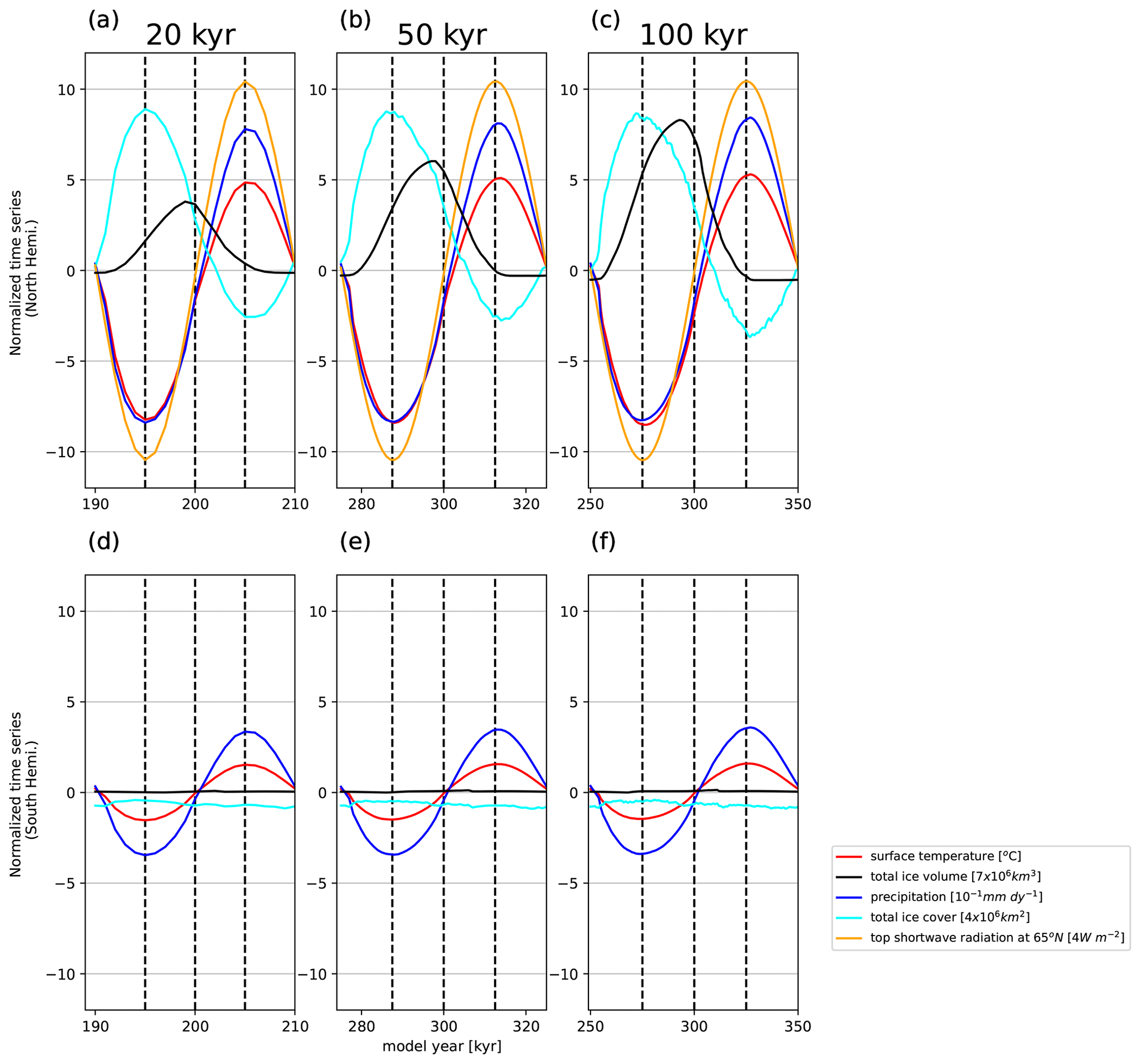
Figure 15Same as Fig. 14 but only for the last cycle of each run. The vertical dashed lines represent the solar forcing sine function phases of −90, 0 and 90∘.
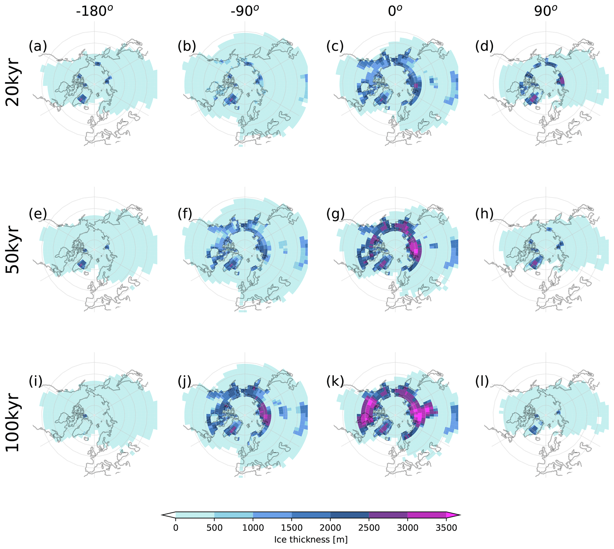
Figure 16Ice thickness (unit: m) distribution in four phases for the forcing periods of 20 kyr (upper), 50 kyr (middle) and 100 kyr (lower) from the last cycle of the shortwave oscillation experiment. The corresponding −180, −90, 0 and 90∘ phase of the solar forcing phases are marked in the headings.
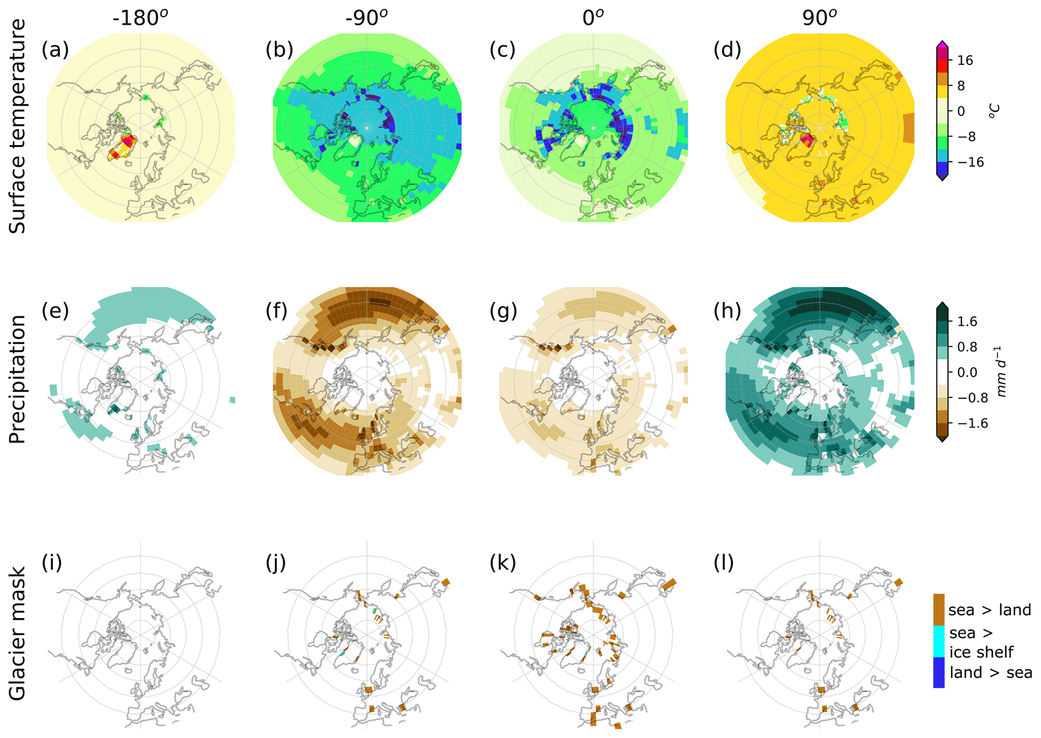
Figure 17Anomalies of surface temperature (upper; unit: ∘C), precipitation (middle; unit: mm d−1) and glacier mask change (lower; brown, cyan and blue represent from ocean to land, from ocean to ice shelf and from land to ocean, respectively) in four phases during the last cycle of the 20 kyr shortwave oscillation experiment. The equilibrium state from coupled dynamic equilibrium experiment is removed to obtain anomalies. The corresponding −180, −90, 0 and 90∘ phase of the solar forcing phases are marked in the headings.
5.2 Shortwave radiation oscillation experiment
In the following experiments we use the same setup as in the previous section but allow the Northern Hemisphere shortwave radiation, sw, to oscillate, taking the following form:
where Asw is the amplitude of the sw oscillations, which increases from 0 at 13∘ N to 0.1 at 35∘ N and maintains 0.1 northward of 35∘ N. The oscillation period, pd, is set to 20, 50 and 100 kyr in three individual simulations. The sw oscillation is relative to the present-day solar radiation, swpresent. The shortwave maximum amplitude is about 20 W m−2 at 65∘ N in the annual mean (Fig. 14a–c) and varies with latitudes and seasons (not shown). The 20, 50 and 100 kyr oscillation periods are simulated for 210, 325 and 350 kyr. The time series for selected climate variables are shown in Fig. 14. The results are shown in reference to the final year of the control run, which is the coupled dynamical equilibrium simulation in Sect. 5.1. To illustrate ice form and retreat in one cycle, we show results from the last forcing cycle of each simulation in Figs. 15–17.
Starting with the 20 kyr oscillation run, there are a number of interesting aspects to point out (Figs. 15a, d, 16a, d and 17a–d). First, at the initial half-cycle, the ice volume is slightly lower than the reference state, indicating a warming period leads to deglaciation (Fig. 14a–c). Then, after the second cycle, the ice volume is always larger than in the control simulation and the cycles are very similar to each other. If we focus on the last cycle of the simulations (Figs. 15–17), we note that Tsurf and precipitation are mostly in phase with each other and with the shortwave radiation forcing. The northern hemispheric Tsurf oscillation amplitude is about ± 6 ∘C, and the mean value is clearly below zero (the control run value). This is despite the fact that the mean shortwave radiation is the same as in the control run. This suggests that the oscillating shortwave radiation has a mean cooling effect. This overall cooling is related to the overall increase in the mean ice sheet volume and extent.
It is beyond this study to fully explore how this effect arises, but it is likely to be related to the ice–albedo effect. In the control run the northern hemispheric summer mean ice cover is nearly zero and, with increasing SW forcing, does not decrease much further. However, it can increase substantially for decreased SW forcing, leading to a mean ice cover in the oscillation run that is much larger than in the control. Subsequently, the northern hemispheric albedo is also much higher than in the control leading to a cooler northern hemispheric Tsurf.
The ice sheet response to the 20 kyr shortwave oscillation has a number of interesting aspects. As mentioned above, the mean ice sheet volume is larger than in the control run. Indeed, it is never smaller than in the control run, not even at the minimum (compare Figs. 13a and 16a), with the exception of the first cycle. Ice-covered regions and ice volume are out of phase. The ice-covered regions (including land snow and sea ice) grow first and are nearly 180∘ out of phase with the SW forcing. The ice sheet volume lags behind the ice-covered area and reaches its maximum nearly 90∘ (a quarter cycle) after the minimum in shortwave radiation (Fig. 15a). This illustrates that the ice sheets have not had enough time to equilibrate with the sw forcing. Further, we can notice that the ice sheet growth and decay is asymmetric, with a slower buildup and faster decay in ice volume, with the reverse pattern in ice sheet area. In the buildup phase the ice sheet extends over large regions at lower latitudes but has relatively thin ice (Fig. 16b). In the decaying phase the ice sheets retreat to higher latitudes and the ice sheet is relatively thick (Fig. 16d).
The northern hemispheric sw forcing also leads to a response in the Southern Hemisphere climate (Fig. 15d). This is mainly due to the GREB-ISM atmospheric heat and moisture transport. It is also partly due to the change in global sea level induced by the northern hemispheric ice sheet changes. The Southern Hemisphere ice sheet changes are in-phase with the Northern Hemisphere climate. It is further noted that the amplitude of the Southern Hemisphere precipitation response relative to Tsurf is bigger than in the Northern Hemisphere (compare Fig. 15a and d; given the same scaling factors). This suggests that the moisture transport is more affected by the northern hemispheric climate change than the heat transport.
The longer 50 and 100 kyr period runs show a number of changes relative to the 20 kyr run. First, the ice sheet volume amplitudes increase relative to the 20 kyr run, illustrating that the ice sheets are more sensitive to longer time period forcings (Fig. 15a–c). Second, we see a shift of the maximum ice volume closer to the phase of the minimum of the sw forcing, suggesting that the ice sheets become closer to equilibrium with longer period sw forcing. However, even the 100 kyr oscillation run still shows a significant delay in the ice sheet volume extrema relative to the forcing extrema, indicating that the ice sheets are not yet in equilibrium with the forcings. This illustrates that the intrinsic timescales of the northern hemispheric ice sheets are longer than 100 kyr. It is further interesting to note that the ice sheets can extend over shallow oceanic regions, like the Hudson Bay, Bering Strait or Arctic Sea in the Siberian sector (Fig. 16g and k), but at the same time do not extend into deep ocean regions (compare Fig. 1c with Fig. 16g and k).
The increase in ice thickness response for the longer 50 and 100 kyr period runs has, however, little impact on the amplitudes of the Tsurf, precipitation and ice cover response in the Northern Hemisphere, which also occurs in the Southern Hemisphere (Fig. 15e and f). For ice sheets in the Southern Hemisphere, the ice thickness is almost keeping constant, which indicates the Antarctica Ice Sheet in the GREB-ISM is not very sensitive to the orbital forcing in Northern Hemisphere.
In this study we introduced a newly developed global ice sheet model coupled to the GREB model, defining the new model GREB-ISM. The ice sheet is simulated on the global grid fully interacting with the climate simulation on all grid points. The ice sheet mass balance is driven by accumulation of snow, melting by surface heat fluxes and changes due to ice transport. The ice transport follows the shallow ice approximation for grounded ice and shallow shelf approximation for ice shelves. Sea-ice–climate interactions are also included. The GREB-ISM climate simulation interacts with ice sheets through surface temperature, precipitation, albedo, land–sea mask, topography and sea level. To allow for these interactions, the original GREB model was changed by improving the precipitation simulation of land, including a prognostic sea ice thickness scheme; coupling the surface albedo to the ice thickness; allowing variable land topography as function of ice thickness; introducing global sea level variation and associated changes in land–sea masks; and improving the meridional turbulent, atmospheric heat transport. Thus, the new GREB-ISM is a fully coupled atmosphere, ocean, land and ice sheet model.
We evaluated the performance of the stand-alone ice sheet model in a series of idealized and realistic ice sheet model simulations. We conducted simulations following the EISMINT I and II idealized experiments and found that the GREB-ISM ice sheet model performs similarly to other models with some limitations in the simulation of internal ice temperature. In simulations with realistic climate forcing close to the present day, we found that the equilibrium in Greenland and most of the East Antarctic ice thickness distribution is very similar to that observed, but the West Antarctic Ice Sheet gains too much ice. The overall surface ice velocities and associated calving rates of this model are similar to those observed for both Greenland and East Antarctica.
We investigated the West Antarctic Ice Sheet thickness bias, by evaluating whether uncertainties in precipitation and the parameterization of the ice shelf dynamics (basal melting and viscosity) could cause this bias. However, we found that this bias is unlikely to be caused by these limitations alone, and it is likely to also result from other, so far unknown, limitations in the GREB-ISM model. A possible explanation could be the complexity of the topography and land–sea distribution of West Antarctica and Antarctic Peninsula, which is not well resolved in the current model resolution. So, the coarse grid resolution of this model is likely to play a role in this limitation (Cuzzone et al., 2019).
A time-dependent simulation with simplified surface temperature and precipitation forcing of the past 250 kyr illustrated that the GREB-ISM model can produce a realistic ice sheet response for Greenland, North American and Fennoscandian ice sheets, together with sea level variability. The results for the Antarctic Ice Sheet are less conclusive but may be due to the simplified setup of the experiment.
We further conducted a series of coupled GREB-ISM simulations to evaluate the full interaction of all climate elements in the model. The coupled model simulations produce global equilibrium ice sheets and calving rates very similar to those observed for present-day boundary conditions. Much of this success in creating a realistic global ice sheet is related to the fact that the GREB-ISM model works with flux correction of surface temperature and land precipitation. This leads to realistic mass balance estimates for the ice sheets even in a fully interactive coupled simulation.
When forced with idealized, oscillating solar radiation forcing on the Northern Hemisphere with different oscillation periods (20, 50 and 100 kyr) the model responds with growth of large continental ice sheets and clear interactions with the climate system in the Northern and Southern Hemispheres. The simulations illustrated asymmetries in the buildup and decay of large ice sheets in response to periodic forcing, showing that the ice sheets are more sensitive to longer-timescale forcings. These experiments illustrate the potential of this model for exploring such interactions in future studies.
The current version GREB-ISM is a useful tool to explore ice-sheet–climate global interaction in ice-age cycles. First, a globally fully coupled model enables us to explore the interaction between the two hemispheres. Most previous studies only simulate Northern or Southern Hemisphere ice sheets and take the others as prescribed boundary conditions (Ganopolski et al., 2010; Tigchelaar et al., 2019). Second, the model is very cheap and it has a high potential to do a fully coupled transition simulation for glacial cycles and sensitivity test. The previous studies pointed out that the ice sheet in paleoclimate has multiple stable equilibria (Abe-Ouchi et al., 2013). Therefore, the simulation of transitions are necessary for ice-age cycle processes. For instance, only in transition experiments can we see the ice sheet inertia effect that the longer forcing period leads to stronger ice thickness response (e.g., Fig. 15).
In summary, we presented a new model that is suited for the simulations of global-scale climate variability on timescales of 100 kyr and longer. Given the coarse resolution of the model, it may be less suitable for shorter timescale studies. The model is computationally efficient, calculating 100 000 model years of global simulations per day on a desktop computer, allowing the simulation of the whole Quaternary period (2.6 Myr) within 1 month. For simulations of climate and ice sheet variability over the Quaternary period the GREB-ISM model is, as presented here, a good starting point. Further development may include other relevant climate processes, such as the carbon cycle, deep ocean reservoirs, or the ability of the atmosphere and ocean circulation to respond to changes in topography and the climate state, as well as glacial isostatic adjustment. Such further developments are possible within the framework of the GREB-ISM model and will be addressed in future studies.
The GREB-ISM source code, the model input data and a simple user manual are available on Zenodo: https://doi.org/10.5281/zenodo.5831376 (Xie, 2022). The reader can redo the simulations in the paper by following the instruction from README.md. The model license is Creative Commons Attribution 4.0 International.
For ice thickness, the Antarctic data are from MEaSUREs BedMachine Antarctica, Version 2 dataset (Morlighem, 2020; Morlighem et al., 2020), while the Greenland data come from IceBridge BedMachine Greenland, Version 3 (recently, it has been updated to version 4, Morlighem et al., 2017, 2021). Observed ice surface velocity in Antarctica for the model benchmark is from the MEaSURE InSAR-Based Antarctica Ice Velocity Map, Version 2 dataset (Mouginot et al., 2012; Rignot et al., 2011, 2017); observed ice surface velocity in Greenland is from the MEaSUREs Greenland Annual Ice Sheet Velocity Mosaics from SAR and Landsat, Version 1 dataset (Joughin, 2017; Joughin et al., 2010). The sea level proxy data are from SPECMAP dataset (specmap.017, Imbrie et al., 1984; Imbrie and McIntyre, 2006). The some values from Tables 4–7 are from literature sources, which are cited inside the text. The other input data for model simulation are all included in our Zenodo package (https://doi.org/10.5281/zenodo.5831376, Xie, 2022).
The supplement related to this article is available online at: https://doi.org/10.5194/gmd-15-3691-2022-supplement.
ZX developed the new ice sheet model code and together with DD design all benchmark experiments. DD helped modify the model coupling process. FSM and ANM provided ice sheet related data and useful comments on the ice sheet dynamics and simulation.
The contact author has declared that neither they nor their co-authors have any competing interests.
Publisher's note: Copernicus Publications remains neutral with regard to jurisdictional claims in published maps and institutional affiliations.
We really appreciate the helpful comments from two referees. We gratefully acknowledge Ralf Greve of Hokkaido University and Ed Bueler of University of Alaska Fairbanks on their suggestions for ice sheet dynamics and modeling. We also thank Chen-shuo Fan of Monash University and Tao Han of the Institute of Earth Environment, CAS, for useful discussion.
This research has been supported by the Climate Extremes (grant no. CE170100023).
This paper was edited by Heiko Goelzer and reviewed by Sam Sherriff-Tadano and one anonymous referee.
Abe-Ouchi, A., Segawa, T., and Saito, F.: Climatic Conditions for modelling the Northern Hemisphere ice sheets throughout the ice age cycle, Clim. Past, 3, 423–438, https://doi.org/10.5194/cp-3-423-2007, 2007.
Abe-Ouchi, A., Saito, F., Kawamura, K., Raymo, M. E., Okuno, J., Takahashi, K., and Blatter, H.: Insolation-driven 100,000-year glacial cycles and hysteresis of ice-sheet volume, Nature, 500, 190–193, https://doi.org/10.1038/nature12374, 2013.
Adler, R. F., Huffman, G. J., Chang, A., Ferraro, R., Xie, P. P., Janowiak, J., Rudolf, B., Schneider, U., Curtis, S., Bolvin, D., Gruber, A., Susskind, J., Arkin, P., and Nelkin, E.: The version-2 global precipitation climatology project (GPCP) monthly precipitation analysis (1979-present), J. Hydrometeorol., 4, 1147–1167, https://doi.org/10.1175/1525-7541(2003)004<1147:TVGPCP>.0.CO;2, 2003.
Allen, D. J., Douglass, A. R., Rood, R. B., and Guthrie, P. D.: Application of a monotonic upstream-biased transport scheme to three- dimensional constituent transport calculations, Mon. Weather Rev., 119, 2456–2464, https://doi.org/10.1175/1520-0493(1991)119<2456:AOAMUB>2.0.CO;2, 1991.
Bauska, T. K., Brook, E. J., Marcott, S. A., Baggenstos, D., Shackleton, S., Severinghaus, J. P., and Petrenko, V. V.: Controls on Millennial-Scale Atmospheric CO2 Variability During the Last Glacial Period, Geophys. Res. Lett., 45, 7731–7740, https://doi.org/10.1029/2018GL077881, 2018.
Behrangi, A., Gardner, A. S., and Wiese, D. N.: Comparative analysis of snowfall accumulation over Antarctica in light of Ice discharge and gravity observations from space, Environ. Res. Lett., 15, 104010, https://doi.org/10.1088/1748-9326/ab9926, 2020.
Bigg, G. R.: An Estimate of the Flux of Iceberg Calving from Greenland, Arct. Antarct. Alp. Res., 31, 174–178, https://doi.org/10.1080/15230430.1999.12003294, 1999.
Bintanja, R. and Van De Wal, R. S. W.: North American ice-sheet dynamics and the onset of 100,000-year glacial cycles, Nature, 454, 869–872, https://doi.org/10.1038/nature07158, 2008.
Bueler, E. and Brown, J.: Shallow shelf approximation as a “sliding law” in a thermomechanically coupled ice sheet model, J. Geophys. Res.-Sol. Ea., 114, 1–21, https://doi.org/10.1029/2008JF001179, 2009.
Bush, A.: Modelling of late Quaternary climate over Asia: a synthesis, Boreas, 33, 155–163, https://doi.org/10.1111/j.1502-3885.2004.tb01137.x, 2004.
Clark, P. U., Dyke, A. S., Shakun, J. D., Carlson, A. E., Clark, J., Wohlfarth, B., Mitrovica, J. X., Hostetler, S. W., and McCabe, A. M.: The Last Glacial Maximum, Science (80-.), 325, 710–714, https://doi.org/10.1126/science.1172873, 2009.
Cuzzone, J. K., Schlegel, N.-J., Morlighem, M., Larour, E., Briner, J. P., Seroussi, H., and Caron, L.: The impact of model resolution on the simulated Holocene retreat of the southwestern Greenland ice sheet using the Ice Sheet System Model (ISSM), The Cryosphere, 13, 879–893, https://doi.org/10.5194/tc-13-879-2019, 2019.
Dee, D. P., Uppala, S. M., Simmons, A. J., Berrisford, P., Poli, P., Kobayashi, S., Andrae, U., Balmaseda, M. A., Balsamo, G., Bauer, P., Bechtold, P., Beljaars, A. C. M., van de Berg, L., Bidlot, J., Bormann, N., Delsol, C., Dragani, R., Fuentes, M., Geer, A. J., Haimberger, L., Healy, S. B., Hersbach, H., Hólm, E. V., Isaksen, L., Kållberg, P., Köhler, M., Matricardi, M., Mcnally, A. P., Monge-Sanz, B. M., Morcrette, J. J., Park, B. K., Peubey, C., de Rosnay, P., Tavolato, C., Thépaut, J. N., and Vitart, F.: The ERA-Interim reanalysis: Configuration and performance of the data assimilation system, Q. J. Roy. Meteor. Soc., 137, 553–597, https://doi.org/10.1002/qj.828, 2011.
Dommenget, D. and Flöter, J.: Conceptual understanding of climate change with a globally resolved energy balance model, Clim. Dynam., 37, 2143–2165, https://doi.org/10.1007/s00382-011-1026-0, 2011.
Dommenget, D. and Rezny, M.: A Caveat Note on Tuning in the Development of Coupled Climate Models, J. Adv. Model. Earth Sy., 10, 78–97, https://doi.org/10.1002/2017MS000947, 2018.
Dommenget, D., Nice, K., Bayr, T., Kasang, D., Stassen, C., and Rezny, M.: The Monash Simple Climate Model experiments (MSCM-DB v1.0): an interactive database of mean climate, climate change, and scenario simulations, Geosci. Model Dev., 12, 2155–2179, https://doi.org/10.5194/gmd-12-2155-2019, 2019.
Fairbanks, G.: A 17,000-year glacio-eustatic sea level record: influence of glacial melting rates on the Younger Dryas event and deep-ocean circulation, Nature, 342, 637–642, 1989.
Felzer, B., Oglesby, R. J., Webb, T., and Hyman, D. E.: Sensitivity of a general circulation model to changes in Northern Hemisphere ice sheets, J. Geophys. Res.-Atmos., 101, 19077–19092, https://doi.org/10.1029/96jd01219, 1996.
Fyke, J. G., Weaver, A. J., Pollard, D., Eby, M., Carter, L., and Mackintosh, A.: A new coupled ice sheet/climate model: description and sensitivity to model physics under Eemian, Last Glacial Maximum, late Holocene and modern climate conditions, Geosci. Model Dev., 4, 117–136, https://doi.org/10.5194/gmd-4-117-2011, 2011.
Ganopolski, A. and Brovkin, V.: Simulation of climate, ice sheets and CO2 evolution during the last four glacial cycles with an Earth system model of intermediate complexity, Clim. Past, 13, 1695–1716, https://doi.org/10.5194/cp-13-1695-2017, 2017.
Ganopolski, A., Calov, R., and Claussen, M.: Simulation of the last glacial cycle with a coupled climate ice-sheet model of intermediate complexity, Clim. Past, 6, 229–244, https://doi.org/10.5194/cp-6-229-2010, 2010.
Gates, W. L.: Modeling the Ice-Age Climate, Science (80-.), 191, 1138–1144, https://doi.org/10.1126/science.191.4232.1138, 1976.
Glen, J. W.: Rate of flow of polycrystalline ice, Nature, 172, 721–722, https://doi.org/10.1038/172721a0, 1953.
Glen, J. W.: The Stability of Ice-Dammed Lakes and other Water-Filled Holes in Glaciers, J. Glaciol., 2, 316–318, https://doi.org/10.3189/s0022143000025132, 1954.
Glen, J. W.: The creep of polycrystalline ice, P. Roy. Soc. Lond. A. Math., 228, 519–538, https://doi.org/10.1098/rspa.1955.0066, 1955.
Greve, R.: Application of a polythermal three-dimensional ice sheet model to the Greenland Ice Sheet: Response to steady-state and transient climate scenarios, J. Climate, 10, 901–918, https://doi.org/10.1175/1520-0442(1997)010<0901:AOAPTD>2.0.CO;2, 1997.
Greve, R. and Blatter, H.: Dynamics of Ice Sheets and Glaciers, Springer, Berlin, ISBN: 9027714738, 2009.
Hildebrand, F. B.: Introduction to Numerical Analysis, Courier Corporation, North Chelmsford, ISBN: 0486653633, 1987.
Hock, R.: Glacier melt: A review of processes and their modelling, Prog. Phys. Geog., 29, 362–391, https://doi.org/10.1191/0309133305pp453ra, 2005.
Hogg, A. M. C.: Glacial cycles and carbon dioxide: A conceptual model, Geophys. Res. Lett., 35, 1–5, https://doi.org/10.1029/2007GL032071, 2008.
Hutter, K.: Theoretical glaciology. Material science of ice and the mechanics of glaciers and ice sheets, Reidel, Dordrecht, Netherlands, ISBN: 9789027714732, 1983.
Huybers, P.: Combined obliquity and precession pacing of late Pleistocene deglaciations, Nature, 480, 229–232, https://doi.org/10.1038/nature10626, 2011.
Huybrechts, P.: Sea-level changes at the LGM from ice-dynamic reconstructions of the Greenland and Antarctic ice sheets during the glacial cycles, Quaternary Sci. Rev., 21, 203–231, https://doi.org/10.1016/S0277-3791(01)00082-8, 2002.
Huybrechts, P., Payne, T., Abe-Ouchi, A., Calov, R., Fabre, A., Fastook, J. L., Greve, R., Hindmarsh, R. C. A., Hoydal, O., Jóhannesson, T., MacAyeal, D. R., Marsiat, I., Ritz, C., Verbitsky, M. Y., Waddington, E. D., and Warner, R.: The EISMINT benchmarks for testing ice-sheet models, Ann. Glaciol., 23, 1–12, https://doi.org/10.3189/s0260305500013197, 1996.
Imbrie, J. and McIntyre, A.: SPECMAP time scale developed by Imbrie et al., 1984 based on normalized planktonic records (normalized O-18 vs time, specmap.017), PANGAEA [data set], https://doi.org/10.1594/PANGAEA.441706, 2006.
Imbrie, J., Hays, J. D., Martinson, D. G., McIntyre, A., Mix, A. C., Morley, J. J., Pisias, N. G., Prell, W. L., and Shackleton, N. J.: The orbital theory of Pleistocene climate: support from a revised chronology of the marine δ18O record, in: Milankovitch and Climate, edited by: Berger, A., Imbrie, J., Hays, H., Kukla, G., and Saltzman, B., Part I. D. Reidel Publishing, Dordrecht, 269–305, 1984.
Irvine, P. J., Gregoire, L. J., Lunt, D. J., and Valdes, P. J.: An efficient method to generate a perturbed parameter ensemble of a fully coupled AOGCM without flux-adjustment, Geosci. Model Dev., 6, 1447–1462, https://doi.org/10.5194/gmd-6-1447-2013, 2013.
Johnsen, S., Clausen, H. B., Dansgaard, W., Gundestrup, N. S., Hammer, C. U., Andersen, U., Andersen, K. K., Hvidberg, C. S., Steffensen, P., White, J., Jouzel, J., and Fisher, D.: core and the problem of possible Eemian climatic instability, J. Geophys. Res., 102, 26397–26410, 1997.
Joughin, I.: MEaSUREs greenland annual ice sheet velocity mosaics from sar and landsat, version 1 [data], NASA Natl. Snow Ice Data Cent. Distrib. Act. Arch. Center [data set], Boulder, Color., USA, https://doi.org/10.5067/OBXCG75U7540, 2017.
Joughin, I., Smith, B. E., Howat, I. M., Scambos, T., and Moon, T.: Greenland flow variability from ice-sheet-wide velocity mapping, J. Glaciol., 56, 415–430, https://doi.org/10.3189/002214310792447734, 2010.
Kageyama, M., Albani, S., Braconnot, P., Harrison, S. P., Hopcroft, P. O., Ivanovic, R. F., Lambert, F., Marti, O., Peltier, W. R., Peterschmitt, J.-Y., Roche, D. M., Tarasov, L., Zhang, X., Brady, E. C., Haywood, A. M., LeGrande, A. N., Lunt, D. J., Mahowald, N. M., Mikolajewicz, U., Nisancioglu, K. H., Otto-Bliesner, B. L., Renssen, H., Tomas, R. A., Zhang, Q., Abe-Ouchi, A., Bartlein, P. J., Cao, J., Li, Q., Lohmann, G., Ohgaito, R., Shi, X., Volodin, E., Yoshida, K., Zhang, X., and Zheng, W.: The PMIP4 contribution to CMIP6 – Part 4: Scientific objectives and experimental design of the PMIP4-CMIP6 Last Glacial Maximum experiments and PMIP4 sensitivity experiments, Geosci. Model Dev., 10, 4035–4055, https://doi.org/10.5194/gmd-10-4035-2017, 2017.
Kalnay, E., Collins, W., Deaven, D., Gandin, L., Iredell, M., Jenne, R., and Joseph, D.: The NCEP/NCAR 40-year reanalysis project, B. Am. Meteorol. Soc., 77, 437–472, https://doi.org/10.1175/1520-0477(1996)077<0437:TNYRP>.0.CO;2, 1996.
Kanamitsu, M., Ebisuzaki, W., Woollen, J., Yang, S. K., Hnilo, J. J., Fiorino, M., and Potter, G. L.: NCEP-DOE AMIP-II reanalysis (R-2), B. Am. Meteorol. Soc., 83, 1631–1644, https://doi.org/10.1175/bams-83-11-1631, 2002.
Lambeck, K., Rouby, H., Purcell, A., Sun, Y., and Sambridge, M.: Sea level and global ice volumes from the Last Glacial Maximum to the Holocene, P. Natl. Acad. Sci. USA, 111, 15296–15303, https://doi.org/10.1073/pnas.1411762111, 2014.
Larour, E., Seroussi, H., Morlighem, M., and Rignot, E.: Continental scale, high order, high spatial resolution, ice sheet modeling using the Ice Sheet System Model (ISSM), J. Geophys. Res.-Earth, 117, https://doi.org/10.1029/2011JF002140, 2012.
Lin, S. J. and Rood, R. B.: An explicit flux-form semi-Lagrangian shallow-water model on the sphere, Q. J. Roy. Meteor. Soc., 123, 2477–2498, https://doi.org/10.1002/qj.49712354416, 1997.
Liu, Y., Moore, J. C., Cheng, X., Gladstone, R. M., Bassis, J. N., Liu, H., Wen, J., and Hui, F.: Ocean-driven thinning enhances iceberg calving and retreat of Antarctic ice shelves, P. Natl. Acad. Sci. USA, 112, 3263–3268, https://doi.org/10.1073/pnas.1415137112, 2015.
Lorbacher, K., Dommenget, D., Niiler, P. P., and Köhl, A.: Ocean mixed layer depth: A subsurface proxy of ocean-atmosphere variability, J. Geophys. Res.-Oceans, 111, 1–22, https://doi.org/10.1029/2003JC002157, 2006.
Macayeal, D. R.: Large-scale ice flow over a viscous basal sediment: theory and application to ice stream B, Antarctica, J. Geophys. Res., 94, 4071–4087, https://doi.org/10.1029/jb094ib04p04071, 1989.
Manabe, S. and Broccoli, A. J.: The Influence of Continental Ice Sheets on the Climate of an Ice Age, J. Geophys. Res., 90, 2167–2190, https://doi.org/10.1029/JD090iD01p02167, 1985.
Martin, M. A., Winkelmann, R., Haseloff, M., Albrecht, T., Bueler, E., Khroulev, C., and Levermann, A.: The Potsdam Parallel Ice Sheet Model (PISM-PIK) – Part 2: Dynamic equilibrium simulation of the Antarctic ice sheet, The Cryosphere, 5, 727–740, https://doi.org/10.5194/tc-5-727-2011, 2011.
Milankovitch, M.: Kanon der Erdbestrahlung und seine Anwendung auf das Eiszeitenproblem, Königliche Serbische Akad., Belgrade, 1941.
Mix, A. C., Bard, E., and Schneider, R.: Environmental processes of the ice age: Land, oceans, glaciers (EPILOG), Quaternary Sci. Rev., 20, 627–657, https://doi.org/10.1016/S0277-3791(00)00145-1, 2001.
Morland, L. W.: Thermomechanical Balances of Ice Sheet Flows, Geophys. Astro. Fluid, 29, 237–266, https://doi.org/10.1080/03091928408248191, 1984.
Morlighem, M.: MEaSUREs BedMachine Antarctica, Version 2 [data], NASA Natl. Snow Ice Data Cent. Distrib. Act. Arch. Center [data set], Boulder, Color., USA, https://doi.org/10.5067/E1QL9HFQ7A8M, 2020.
Morlighem, M., Williams, C. N., Rignot, E., An, L., Arndt, J. E., Bamber, J. L., Catania, G., Chauché, N., Dowdeswell, J. A., Dorschel, B., Fenty, I., Hogan, K., Howat, I., Hubbard, A., Jakobsson, M., Jordan, T. M., Kjeldsen, K. K., Millan, R., Mayer, L., Mouginot, J., Noël, B. P. Y., O'Cofaigh, C., Palmer, S., Rysgaard, S., Seroussi, H., Siegert, M. J., Slabon, P., Straneo, F., van den Broeke, M. R., Weinrebe, W., Wood, M., and Zinglersen, K. B.: BedMachine v3: Complete Bed Topography and Ocean Bathymetry Mapping of Greenland From Multibeam Echo Sounding Combined With Mass Conservation, Geophys. Res. Lett., 44, 11051–11061, https://doi.org/10.1002/2017GL074954, 2017.
Morlighem, M., Rignot, E., Binder, T., Blankenship, D., Drews, R., Eagles, G., Eisen, O., Ferraccioli, F., Forsberg, R., Fretwell, P., Goel, V., Greenbaum, J. S., Gudmundsson, H., Guo, J., Helm, V., Hofstede, C., Howat, I., Humbert, A., Jokat, W., Karlsson, N. B., Lee, W. S., Matsuoka, K., Millan, R., Mouginot, J., Paden, J., Pattyn, F., Roberts, J., Rosier, S., Ruppel, A., Seroussi, H., Smith, E. C., Steinhage, D., Sun, B., van den Broeke, M. R., van Ommen, T. D., van Wessem, M., and Young, D. A.: Deep glacial troughs and stabilizing ridges unveiled beneath the margins of the Antarctic ice sheet, Nat. Geosci., 13, 132–137, https://doi.org/10.1038/s41561-019-0510-8, 2020.
Morlighem, M., Williams, C., Rignot, E., An, L., Arndt, J. E., Bamber, J., Catania, G., Chauché, N., Dowdeswell, J. A., Dorschel, B., Fenty, I., Hogan, K., Howat, I., Hubbard, A., Jakobsson, M., Jordan, T. M., Kjeldsen, K. K., Millan, R., Mayer, L., Mouginot, J., Noël, B., O'Cofaigh, C., Palmer, S. J., Rysgaard, S., Seroussi, H., Siegert, M. J., Slabon, P., Straneo, F., van den Broeke, M. R., Weinrebe, W., Wood, M., and Zinglersen, K.: IceBridge BedMachine Greenland, Version 4. [data], NASA Natl. Snow Ice Data Cent. Distrib. Act. Arch. Center [data set], Boulder, Color., USA, https://doi.org/10.5067/VLJ5YXKCNGXO, 2021.
Mouginot, J., Scheuch, B., and Rignot, E.: Mapping of ice motion in antarctica using synthetic-aperture radar data, Remote Sens.-Basel, 4, 2753–2767, https://doi.org/10.3390/rs4092753, 2012.
Niu, L., Lohmann, G., Hinck, S., Gowan, E. J., and Krebs-Kanzow, U.: The sensitivity of Northern Hemisphere ice sheets to atmospheric forcing during the last glacial cycle using PMIP3 models, J. Glaciol., 65, 645–661, https://doi.org/10.1017/jog.2019.42, 2019.
Overpeck, J. T., Otto-Bliesner, B. L., Miller, G. H., Muhs, D. R., Alley, R. B., and Kiehl, J. T.: Paleoclimatic evidence for future ice-sheet instability and rapid sea-level rise, Science (80-.), 311, 1747–1750, https://doi.org/10.1126/science.1115159, 2006.
Payne, A. J., Huybrechts, P., Abe-Ouchi, A., Calov, R., Fastook, J. L., Greve, R., Marshall, S. J., Marsiat, I., Ritz, C., Tarasov, L., and Thomassen, M. P. A.: Results from the EISMINT model intercomparison: The effects of thermomechanical coupling, J. Glaciol., 46, 227–238, https://doi.org/10.3189/172756500781832891, 2000.
Pollard, D. and DeConto, R. M.: Description of a hybrid ice sheet-shelf model, and application to Antarctica, Geosci. Model Dev., 5, 1273–1295, https://doi.org/10.5194/gmd-5-1273-2012, 2012.
Rayner, N. A., Parker, D. E., Horton, E. B., Folland, C. K., Alexander, L. V., Rowell, D. P., Kent, E. C., and Kaplan, A.: Global analyses of sea surface temperature, sea ice, and night marine air temperature since the late nineteenth century, J. Geophys. Res.-Atmos., 108, 4407, https://doi.org/10.1029/2002jd002670, 2003.
Rignot, E., Mouginot, J., and Scheuchl, B.: Ice flow of the antarctic ice sheet, Science, 333, 1427–1430, https://doi.org/10.1126/science.1208336, 2011.
Rignot, E., Mouginot, J., and Scheuchl, B.: MEaSUREs InSAR-based Antarctica ice velocity map, version 2, NASA Natl. Snow Ice Data Cent. Distrib. Act. Arch. Center [data set], Boulder, Color., USA, https://doi.org/10.5067/D7GK8F5J8M8R, 2017.
Robinson, D., David, A., Estilow, T., and Program, N. C.: NOAA Climate Date Record (CDR) of Northern Hemisphere (NH) Snow Cover Extent (SCE), Version 1, NOAA Natl. Clim. Data Cent., 137–142, https://doi.org/10.7289/V5N014G9, 2012.
Rossow, W. B. and Schiffer, R. A.: ISCCP cloud data products, B. Am. Meteorol. Soc., 72, 2–20, https://doi.org/10.1175/1520-0477(1991)072<0002:ICDP>2.0.CO;2, 1991.
Schneider, E. K.: Flux correction and the simulation of changing climate, Ann. Geophys., 14, 336–341, https://doi.org/10.1007/s00585-996-0336-8, 1996.
Shackelton, N. J.: The 100,000-year ice-age cycle identified and found to lag temperature, carbon dioxide, and orbital eccentricity, Science (80-.), 289, 1897–1902, https://doi.org/10.1126/science.289.5486.1897, 2000.
Shi, X., Yang, H., Danek, C., and Lohmann, G.: AWI AWI-ESM1.1LR model output prepared for CMIP6 PMIP, Earth System Grid Federation [data set], https://doi.org/10.22033/ESGF/CMIP6.9302, 2020.
Short, D. A., Mengel, J. G., Crowley, T. J., Hyde, W. T., and North, G. R.: Filtering of Milankovitch Cycles by Earth's Geography, Quaernary Res., 35, 157–173, https://doi.org/10.1016/0033-5894(91)90064-c, 1991.
Stassen, C., Dommenget, D., and Loveday, N.: A hydrological cycle model for the Globally Resolved Energy Balance (GREB) model v1.0, Geosci. Model Dev., 12, 425–440, https://doi.org/10.5194/gmd-12-425-2019, 2019.
Suarez, M. J. and Takacs, L. L.: Technical report series on global modeling and data assimilation. Volume 5: Documentation of the ARIES/GEOS dynamical core, version 2, NASA Technical Memorandum 104606, Vol. 5, 1995.
Tabor, C. R., Poulsen, C. J., and Pollard, D.: How obliquity cycles powered early Pleistocene global ice-volume variability, Geophys. Res. Lett., 42, 1871–1879, https://doi.org/10.1002/2015GL063322, 2015.
Tigchelaar, M., Timmermann, A., Friedrich, T., Heinemann, M., and Pollard, D.: Nonlinear response of the Antarctic Ice Sheet to late Quaternary sea level and climate forcing, The Cryosphere, 13, 2615–2631, https://doi.org/10.5194/tc-13-2615-2019, 2019.
Velichko, A. A., Kononov, Y. M., and Faustova, M. A.: The last glaciation of earth: Size and volume of ice-sheets, Quatern. Int., 41–42, 43–51, https://doi.org/10.1016/s1040-6182(96)00035-3, 1997.
Webb, T., Anderson, K. H., Bartlein, P. J., and Webb, R. S.: Late Quaternary climate change in eastern North America: A comparison of pollen-derived estimates with climate model results, Quaternary Sci. Rev., 17, 587–606, https://doi.org/10.1016/S0277-3791(98)00013-4, 1998.
Willeit, M., Ganopolski, A., Calov, R., and Brovkin, V.: Mid-Pleistocene transition in glacial cycles explained by declining CO2 and regolith removal, Sci. Adv., 5, 1–9, https://doi.org/10.1126/sciadv.aav7337, 2019.
Wunsch, C.: Quantitative estimate of the Milankovitch-forced contribution to observed Quaternary climate change, Quaternary Sci. Rev., 23, 1001–1012, https://doi.org/10.1016/j.quascirev.2004.02.014, 2004.
Xie, Z.: YMI33/GREB-ISM: GREB-ISM with forcing from LGM experiment (v1.0), Zenodo [code], https://doi.org/10.5281/zenodo.5831376, 2022.
- Abstract
- Introduction
- Data
- Model description
- Model benchmark: ice sheet model stand-alone simulations
- Model benchmark: GREB-ISM coupled simulations
- Summary and discussion
- Code availability
- Data availability
- Author contributions
- Competing interests
- Disclaimer
- Acknowledgements
- Financial support
- Review statement
- References
- Supplement