Assessment of the sea surface temperature diurnal cycle in CNRM-CM6-1 based on its 1D coupled configuration

A single-column version of the CNRM-CM6-1 global climate model has been developed to ease development and validation of the boundary layer physics and air–sea coupling in a simplified environment. This framework is then used to assess the ability of the coupled model to represent the sea surface temperature (SST) diurnal cycle. To this aim, the atmospheric–ocean single-column model (AOSCM), called CNRM-CM6-1D, is implemented in a case study derived from the CINDY2011/DYNAMO campaign over the Indian Ocean, where large diurnal SST variabilities have been well documented.

Comparing the AOSCM and its uncoupled components (atmospheric SCM and oceanic SCM, called OSCM) highlights the fact that the impact of coupling in the atmosphere results from both the possibility to take into account the diurnal variability of SST, which is not usually available in forcing products, and the change in mean state SST as simulated by the OSCM, with the ocean mean state not being heavily impacted by the coupling. This suggests that coupling feedbacks in the 3D model do not arise from the coupling of ocean and atmosphere vertical column physics but are more due to the large-scale dynamics resolved by the 3D model. Additionally, a sub-daily coupling frequency is needed to represent the SST diurnal variability, but the choice of the coupling time step between 15 min and 3 h does not impact the diurnal temperature range simulated much. The main drawback of a 3 h coupling is delaying the SST diurnal cycle by 5 h in asynchronous coupled models. Overall, the diurnal SST variability is reasonably well represented in CNRM-CM6-1 with a 1 h coupling time step and the upper-ocean model resolution of 1 m.

This framework is shown to be a very valuable tool to develop and validate the boundary layer physics and the coupling interface. It highlights the interest to develop other atmosphere–ocean coupling case studies.

1 Introduction

Because of the many interactions and feedbacks occurring in a general circulation model (GCM), either between parameterizations or between the parameterized subgrid processes and the resolved dynamics (e.g., Bhattacharya et al., 2018), understanding their behavior or the origin of their systematic errors is often complex. The latter task is even more complicated when GCMs are coupled together (e.g., as in ocean–atmosphere models). In the history of GCM development, simplified versions of GCMs, such as a single-column model (SCM) consisting of a single grid column of the host GCM, have therefore been widely used (e.g., Betts and Miller, 1986; Price et al., 1986; Gaspar et al., 1990; Randall et al., 1996; Hourdin et al., 2017; Giordani et al., 2020). Such modeling frameworks ease the development of parameterizations as the resolved dynamics are fully controlled and do not interact with the simulated subgrid processes (Randall et al., 1996; Randall and Cripe, 1999). Also, SCMs have the great advantage of being computationally very cheap, enabling their use on personal computers and allowing modelers to rapidly test their ideas and perform numerous sensitivity tests. The reduced set of interactions and feedbacks in SCMs compared to the host GCM, and the possibility to output many diagnostics at model time steps on the model vertical grid, also helps the modeler to better tackle the cause-and-effect relationship among the parameterized processes and thereby identify model deficiencies. A large number of SCM intercomparisons either for atmospheric SCMs (e.g., Bechtold et al., 1996; Lenderink et al., 2004; Guichard et al., 2004; Cuxart et al., 2006; Klein et al., 2009; Davies et al., 2013; Couvreux et al., 2015) or oceanic SCMs (Acreman and Jeffery, 2007; Damerell et al., 2020; Reffray et al., 2015) have helped to improve the model parameterizations. This effort has been possible thanks to the availability of high-resolution simulations as a reference (e.g., Randall et al., 1996; Couvreux et al., 2021, and references therein).

SCMs of either the atmosphere or the ocean often require constraints of large-scale circulations and boundary conditions at the surface. Over ocean surfaces, atmospheric SCMs are often used with a prescribed sea surface temperature (e.g., Chlond et al., 2004; Neggers et al., 2017) or with prescribed surface fluxes (e.g., Abdel-Lathif et al., 2018). This implies no feedback of the simulated atmosphere on the surface boundary condition, as is the case in the real ocean–atmosphere system, and thus limits the potential use of SCMs in conditions in which the ocean–atmosphere coupling is critical. Similar limitations are also found over land, even though the use of atmospheric SCMs coupled to a land surface model is more common (e.g., Giordani et al., 1996; Bosveld et al., 2014). In the case of oceanic SCMs, the boundary conditions are similarly provided by prescribing either the atmospheric near-surface parameters or the surface fluxes. Prescribing atmospheric surface parameters induces a strong restoring of the sea surface temperature through the turbulent heat flux bulk parameterization and thus strongly constrains the ocean mixed layer heat content. Prescribing surface fluxes appears to be a good alternative, but surface fluxes are not directly measured and estimations are always uncertain. In addition, prescribed surface fluxes do not account for the thermal adjustment of the atmospheric boundary layer to the sea surface conditions (e.g., Barnier et al., 1995). To overcome these caveats and properly study the interplay between the atmosphere and ocean boundary layers, only a few studies have so far developed coupled ocean–atmosphere SCMs (Clayson and Chen, 2002; Deppenmeier et al., 2020; Hartung et al., 2018).

The present work seeks to reduce this gap by developing the atmosphere–ocean SCM (AOSCM) version of the CNRM-CM6-1 climate model (Voldoire et al., 2019). To remain as relevant as possible to its 3D counterpart, both scientifically and technically, the AOSCM is developed while keeping most of the 3D model technical framework, in particular its coupling interface. Such an AOSCM is also a practicable tool to better understand the coupled ocean–atmosphere feedbacks, enabling modelers to disentangle the role of the dynamics from the model physics.

Among ocean–atmosphere coupled processes, the SST diurnal cycle is of special interest and has been the subject of active research over the past decade. Diurnal warm-layer anomalies can reach up to 5 ^∘C in the tropics (Ward, 2006; Wick and Castro, 2020) and have been shown to impact on the atmospheric and oceanic mean state (Itterly et al., 2021; Li et al., 2020) as well as on climate variability, in particular the Madden–Julian oscillation (MJO; Bernie et al., 2008; Seo et al., 2014). Bernie et al. (2005, 2008) highlight a rectification effect of the diurnal SST variability on the mean state: the daily maximum SST is increased as is the upper-ocean stratification, which further increases the upper-layer heat uptake in the following days, leading to a persistent SST warming that can modify the monthly mean SST.

The ability of our GCM to represent this diurnal variability and its impact on the atmospheric and oceanic boundary layers is of interest but difficult to validate in 3D configurations. We therefore take advantage of the AOSCM framework to better understand the ability of the CNRM-CM6-1 atmospheric and ocean vertical physics to represent diurnal oceanic warm layers in the tropics. In this regard, an AOSCM case study based on the Cooperative Indian Ocean Experiment on Intraseasonal Variability in the Year 2011 (CINDY2011)/Dynamics of the MJO (DYNAMO) field campaign (Yoneyama et al., 2013) is developed and serves to highlight the features of the model configuration key to properly capture the SST diurnal cycle. Following previous studies (e.g., Bernie et al., 2008; Ma and Jiang, 2021), the roles of the vertical resolution in the upper ocean and of the atmosphere–ocean coupling frequency are emphasized.

Section 2 describes the CNRM-CM6-1 AOSCM, which is referred to as CNRM-CM6-1D hereafter. Based on the CINDY2011/DYNAMO field campaign and other related data, Sect. 3 develops the forcing appropriate for an AOSCM case study. It also introduces the data used as a reference for analysis. Section 4 discusses the representation of the SST diurnal cycle in either atmospheric or oceanic stand-alone versions of the AOSCM, while Sect. 5 fully makes use of the coupled AOSCM to assess its ability to represent the SST diurnal cycle and how this representation depends on the AOSCM configuration. Section 6 concludes this work.

2 Model description

The objective of this work is to develop a single-column version of the climate model CNRM-CM6-1, the CMIP6 version of the CNRM-CM model (Voldoire et al., 2019). This model is composed of ARPEGE 6.3 (Roehrig et al., 2020) for the atmosphere, NEMO3.6 (Madec et al., 2017) for the ocean, SURFEX v8 for the land processes and ocean surface fluxes (Decharme et al., 2019), CTRIP for river routing, and GELATO 6 for the sea ice. These components are coupled through OASIS3-MCT (Craig et al., 2017). To derive a single-column version, we use the SCM version of ARPEGE that has been extensively used to develop and test atmospheric parameterizations (e.g., Abdel-Lathif et al., 2018; Roehrig et al., 2020). The atmospheric SCM uses SURFEX to represent the land surface processes or to calculate the ocean turbulent surface fluxes, depending on the case properties and SCM setup. An SCM version of NEMO has also been used to develop and test oceanic parameterizations (Giordani et al., 2020; Reffray et al., 2015). In the 3D model, the OASIS coupling interface is implemented within both SURFEX and NEMO (Voldoire et al., 2017). The individual AOSCM components are thus already in place, which eases the development of the fully coupled AOSCM (Fig. 1). Only the CTRIP component, which is fundamentally 2D, is not included in the AOSCM .

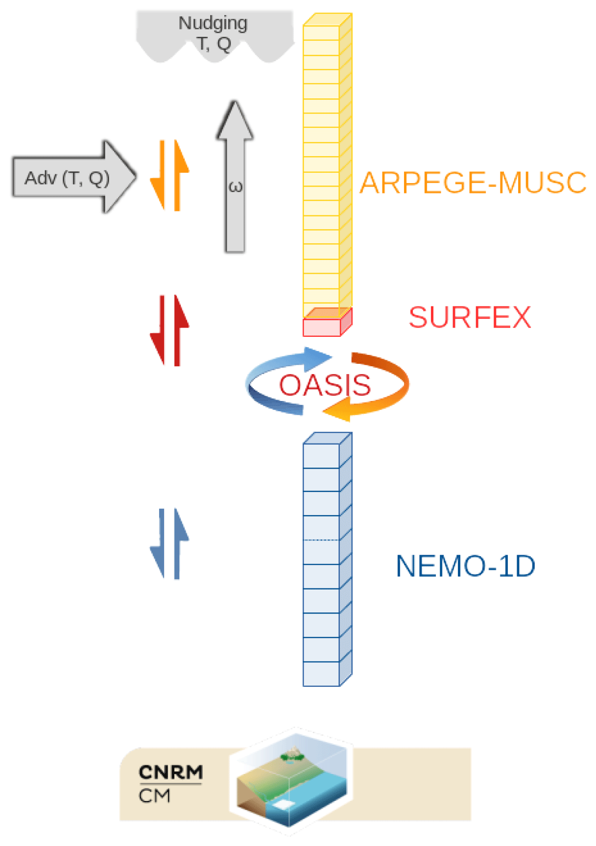
Figure 1 Schematic of the CNRM-CM6-1D uni-column coupled model. The grey elements picture imposed large-scale forcings. ω stands for the vertical velocity in pressure coordinates.

In practice, the ARPEGE-SURFEX SCM consists of four identical grid columns, as it allows the SCM to use the same dynamical core as the regional configuration of ARPEGE (e.g., Nabat et al., 2020). Note that this dynamical core shares the same semi-Lagrangian advection scheme as ARPEGE, while it treats the spectral transforms required by the spectral formulation of the model differently. The vertical advection of the model state variables, when needed, is thus computed as in the 3D model. Similarly, the NEMO SCM uses nine identical grid columns. For a given component, the coupling finally considers a single grid cell and replicates the associated information to transfer it to all grid cells of the other component. Thus OASIS3-MCT does not perform any horizontal interpolation and only provides communication support to the coupling. Keeping OASIS3-MCT in CNRM-CM6-1D ensures full consistency between the AOSCM and its 3D counterpart, in particular with respect to the coupling time sequence. Each individual component integrates its own physics between two coupling time steps at which they exchange the relevant coupling fields. The atmosphere SCM thus receives and uses the sea surface temperature as computed by the ocean SCM at the end of the previous coupling time step, while the ocean SCM receives and uses the surface turbulent fluxes as computed by the atmospheric SCM (SURFEX component) and accumulated during the previous coupling time step (asynchronous coupling). The coupling time step is an OASIS parameter, and in the 3D case, it is fixed to 1 h. In this SCM case study, the impact of choosing a coupling frequency from 5 min to 1 d will be assessed. To be able to disentangle the effect of changing the coupling time step from changing the model component time steps, we have fixed the atmospheric and oceanic time step to 5 min in the SCM to enable the use of a very short coupling time step. It has, however, been determined that changing the component time steps from their default values (15 min in the atmosphere and 30 min in the ocean) to 5 min does not alter the SCM results. In principle, the sea ice model GELATO, which is integrated within NEMO, could be activated in the AOSCM. However, as we focus hereafter on a tropical case study, this has not been tested yet.

In this study, to enable a fair comparison of the oceanic SCM (OSCM) with the AOSCM, we have run the OSCM jointly with the SURFEX platform so as to ensure a common flux computation using the COARE version 3.0 bulk scheme (Fairall et al., 2003).

3 Development of a CINDY2011/DYNAMO AOSCM case

3.1 Selected period and location

The 3-month CINDY2011/DYNAMO field campaign (Yoneyama et al., 2013) was designed to study the Madden–Julian oscillation initiation in the Indian Ocean, in particular interaction with the surface ocean. We take this campaign as an opportunity to develop an AOSCM case permitting us to study the representation of the upper-ocean diurnal cycle, which includes frequent and intense diurnal warm layers over the region (e.g., Kawai and Wada, 2007; Matthews et al., 2014). The field campaign provides a wide variety of measurements, including high-frequency soundings from either local islands or research vessels that were deployed during the campaign, near-surface measurements in the atmosphere and the ocean, and upper-ocean profiles.

Ciesielski et al. (2014) derived the various terms of the mass, energy, and water budgets (e.g., vertical velocity, horizontal advection, sub-array diabatic terms) at the scale of two large-scale arrays (∼ 800 km) over the tropical Indian Ocean. This dataset was used in Abdel-Lathif et al. (2018) to force a previous version of the ARPEGE-SURFEX SCM. In contrast, available ocean data mostly come from the R/V Revelle, which was used as a fixed station at 0^∘ N, 80.5^∘ E for periods of several months. These local data are not sufficient to derive a consistent large-scale forcing of the AOSCM ocean component. We therefore decided to develop a more local AOSCM forcing based on the R/V Revelle data. This case study has been developed in the context of the French research project COCOA and has been used in several studies (Brilouet et al., 2021). The ship's location at the Equator implies possible strong large-scale advection, which needs to be quantified for forcing the AOSCM. This issue is discussed in the next section.

As a result, the AOSCM case developed hereafter focuses on the first 10 d of the R/V Revelle leg 3, i.e., from 13 November 2011 at 00:00 UTC to 23 November 2011 at 00:00 UTC. This period corresponds to a convectively suppressed MJO phase followed by the early beginning of a convectively active phase. A clear motivation for this choice is the occurrence of large SST diurnal cycles during most of this period.

3.2 Reference datasets

To assess the model simulations, we use local observation data from the R/V Revelle. SSTs taken are obtained from the ship's intake thermosalinograph at 5 m depth corrected to represent the skin temperature based on the Sea Snake floating thermistor at 5 cm depth (Edson et al., 2016; de Szoeke et al., 2015). In the following the SST used as a reference will be the SST skin temperature.

Reference turbulent fluxes are obtained from the NOAA PSD (Physical Science Division) and provided by Chris Fairall and Ludovic Bariteau at hourly frequency. Two products are derived from high-frequency field measurements, either computed using eddy covariance (EC) or inertio-dissipative (ID) methods. We also use both conductivity–temperature–depth (CTD) casts and the Oregon State University Chameleon profiler to get ocean temperature and salinity profiles, as well as acoustic Doppler current profiler (ADCP) records to get current profiles (Moum, 2016). The Oregon State University Chameleon profiler also provides profiles of the Brunt–Vaïsala frequency.

Several reanalysis products are also used for both the atmosphere and the ocean. For the ocean, we have used ORAS5 (Zuo et al., 2019) and Glorys2V4 (Ferry et al., 2012). Both have a resolution of 0.25^∘ with a latitudinal refinement to 0.15^∘ near the Equator. For the atmosphere, we have used the ERA-Interim daily data (Dee et al., 2011).

In this study, as we are more interested in the mean behavior of the model in simulating SST diurnal cycles, we have chosen to calculate the mean diurnal temperature range (DTR) as the amplitude of the mean SST cycle averaged over the period of analysis. In practice, DTR is the difference between the maximum and minimum temperature of the mean daily cycle. This choice mainly reduces the values of DTR but does not impact the main outcomes of this study.

3.3 Atmospheric model setup

The AOSCM atmospheric component uses exactly the same physical package as that used in CNRM-CM6-1 (Sect. 2). The vertical discretization is also the same, with 91 vertical levels spanning 10 m to 80 km. The vertical resolution is enhanced in the boundary layer (10 and 100 m below 1 km) (see Fig. 1 in Roehrig et al., 2020).

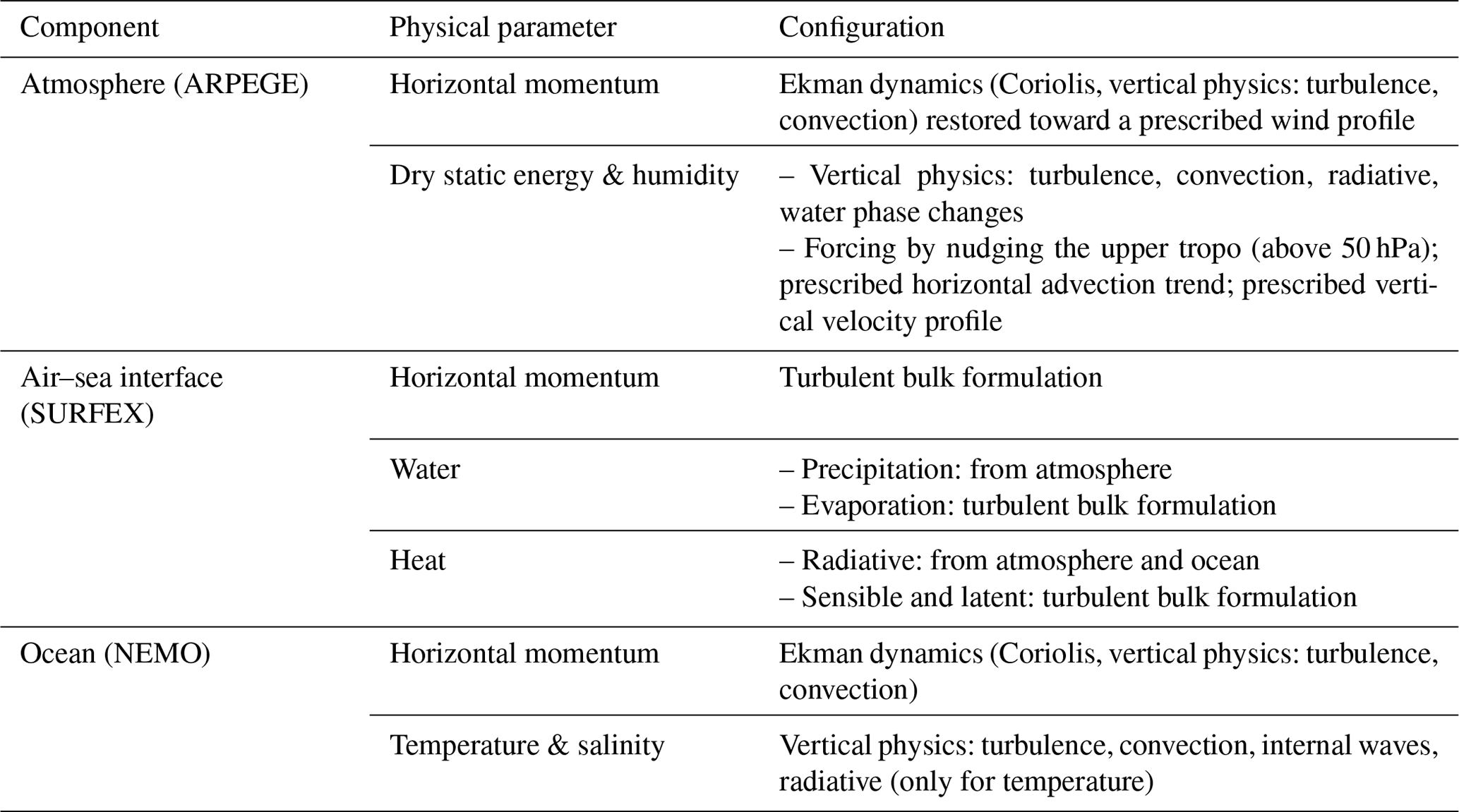
The large-scale atmospheric forcing of the AOSCM is derived from a constrained variational analysis (CVA), following Zhang and Lin (1997), Zhang et al. (2001), and Xie et al. (2004). The CVA assesses the large-scale mass, energy, and moisture budgets at the scale of a 50 km radius disk centered on the R/V Revelle and at the 3-hourly timescale. The 50 km scale is a trade-off between a reduced amount of noise in the forcing and the targeted local scale of the R/V Revelle measurements used hereafter. The CVA uses the European Centre for Medium-Range Weather Forecasts (ECMWF) operational analyses as an input and the surface precipitation measurements retrieved from the Colorado State University's Tropical Ocean Global Atmosphere (TOGA) radar on board the R/V Revelle as a constraint. The CVA provides initial profiles of wind horizontal components, temperature, and specific humidity, as well as the initial surface pressure, which are used to initialize the AOSCM atmospheric component. It also estimates the horizontal advection of temperature and specific humidity as well as the pressure vertical velocity (ω), which are further used as a forcing of the atmospheric column. Using the CVA pressure vertical velocity, the SCM computes its own vertical advection based on the simulated temperature and specific humidity profiles. In contrast, the horizontal wind forcing is more difficult to estimate based on observation-based momentum budgets (e.g., weak geostrophic balance near the Equator). Therefore, the SCM zonal and meridional wind components are simply nudged towards those of the CVA with a 3-hourly nudging timescale. Following Abdel-Lathif et al. (2018), note that the wind, temperature, and moisture profiles are extended above 50 hPa using first the ERA-Interim reanalysis (Dee et al., 2011) up to 1 hPa and then the 1976 US standard atmosphere profile (COESA, 1976 – temperature only, wind and specific humidity being set to zero). Above 50 hPa, the horizontal advection and vertical velocity are set to zero, while temperature and specific humidity are further nudged toward the extended profile. At the surface, the CVA surface pressure is prescribed. In the case of atmosphere-only SCM simulations, the R/V Revelle observed SSTs are imposed, and thus surface fluxes are computed by the SURFEX bulk parameterization. Table 1 summarizes this model physical configuration.

Table 1 Physical configuration of CNRM-CM6-1D.

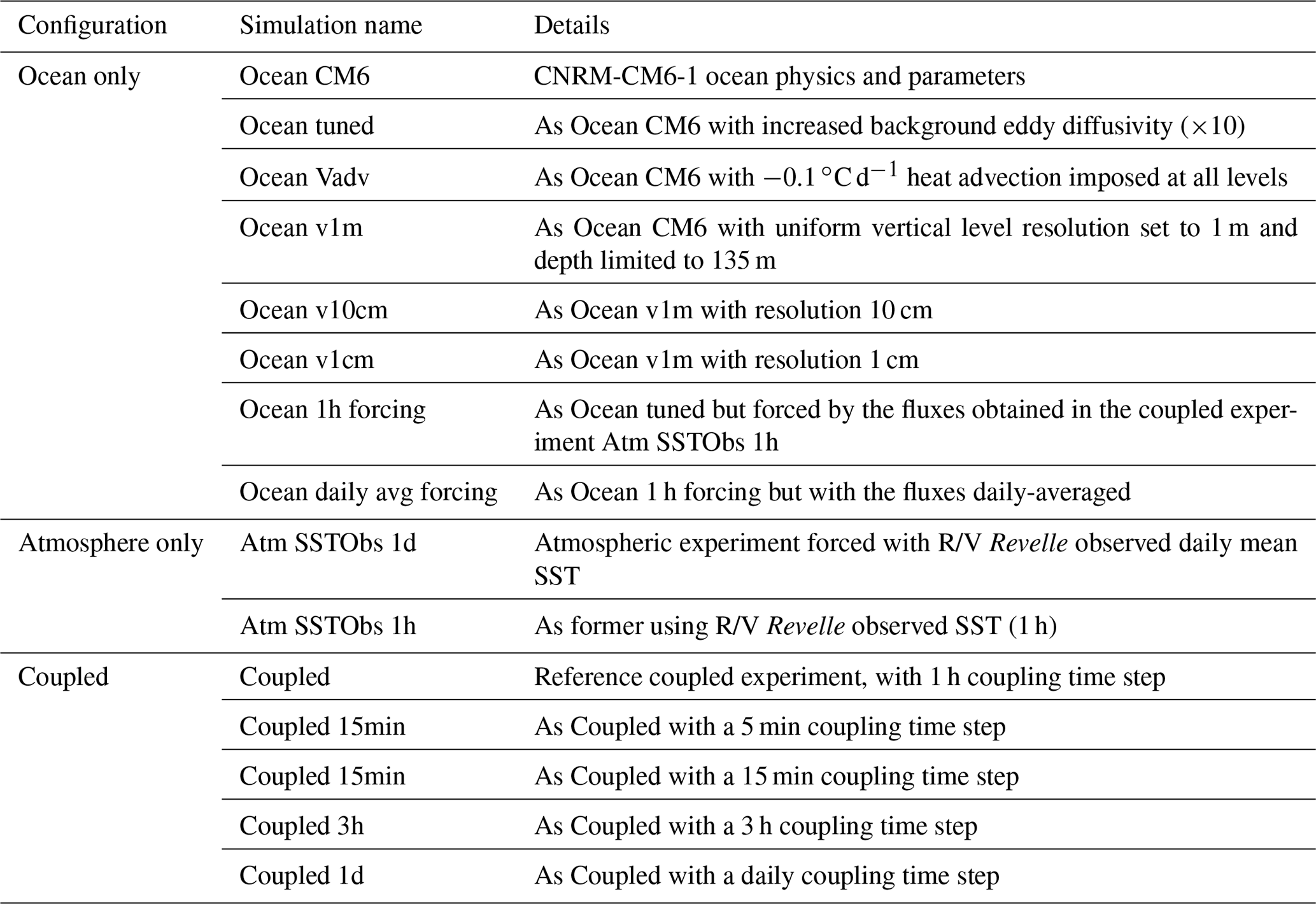
SCM simulations may be strongly constrained by the prescribed forcing. However, the latter often has large uncertainties because of the very few in situ observations, which weakly constrain the input data of the CVA (e.g., the ECMWF analyses) or which more directly enter the CVA algorithm. This may sometimes question the detailed comparison between SCM simulation output and other independent data. As an attempt to address the forcing uncertainties, 10-member ensembles of SCM simulations are performed by introducing weak and random noise in the forcing large-scale advection and vertical velocity fields. This should avoid focusing the upcoming analysis on small, most likely insignificant differences between simulations or between simulations and reference datasets. Note that all experiments discussed hereafter have been listed in Table 2.

Table 2 List of experiments done with CNRM-CM6-1D for each experiment; the table indicates the components involved and a short description.

3.4 Ocean model setup

As for the atmosphere, the ocean configuration is taken from the CNRM-CM6-1 version. The whole set of parameterizations used is listed in Voldoire et al. (2019). Of interest for the present study is that in this configuration, there are 75 vertical levels, with the first layer of 1 m thickness. The ocean vertical mixing of tracers and momentum is parameterized by a turbulent kinetic energy scheme (Blanke and Delecluse, 1993), and the convection is roughly represented by an increase in the coefficient of vertical diffusion for tracers (Lazar et al., 1999) in the case of static instabilities.

To design the ocean column forcing, we use the NEMO single-column version forced by near-surface atmospheric measurements collected on the R/V Revelle at a 10 min frequency, namely air temperature, specific humidity, wind speed, surface pressure, surface precipitation, and surface downwelling longwave and shortwave radiation. The atmospheric forcing is thus representative of the local R/V Revelle scale, which the OSCM simulations are intended to match.

The ocean column state is initialized using in situ CTD data for temperature and salinity and from ADCP measurements for currents. As these observations extend to 250 and 150 m depth, respectively, the ORAS5 reanalysis data are used below these levels. No spurious gradients are generated near the merging depth, as ORAS5 is found to simulate profiles very close to those observed from the R/V Revelle. Moreover, we are mainly interested in the near-surface layers, and these are weakly impacted by the oceanic state below 150 m over the simulated 10 d (not shown).

As a first guess, the ocean SCM is run without imposing any large-scale advection (horizontal nor vertical) using the default CNRM-CM6-1 NEMO configuration (Voldoire et al., 2019). The simulated daily mean SST time series warms during the first 3 d by 0.8 ^∘C and then approximately follows the observed SST time evolution (Fig. 2a, purple versus black lines). The surface warm bias extends up to 10 m, while a cold bias develops below 30 m (Fig. 3a), thus suggesting a lack of downward heat transfer. The mean salinity (Fig. 3b) is accurate to a depth of a few meters. Below about 5 m, the model has a fresh bias of 0.1 psu with respect to the CTD observations, which is, however, within the range of uncertainty as given by the two ocean reanalyses. The Chameleon data collected at the location of the R/V Revelle provide an estimate of the Brunt–Vaïsala frequency vertical profile (Fig. 3c), which is well captured by the OSCM between 100 and 10 m. Above, the model clearly overestimates the stability.

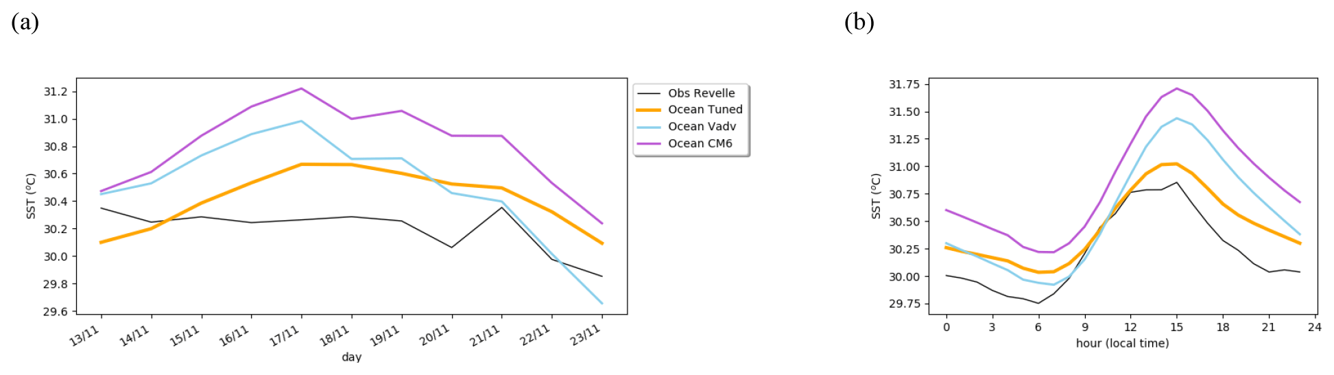
Figure 2 (a) Daily time series and (b) mean diurnal cycle of SST (^∘C) in ocean forced experiments compared to SST measured on the R/V Revelle.

Figure 3 Mean vertical profile of (a) temperature (^∘C), (b) salinity (psu), and (c) the Brunt–Vaïsala frequency (10⁻⁴ s⁻²) averaged over the simulated period (13–22 November).

Several deficiencies may explain the OSCM warm bias in the upper ocean: deficiencies in the OSCM forcing setup such as a missing large-scale advection term or underestimated current that does not generate enough turbulence, deficiencies in the OSCM physics, such as a flaw in the vertical mixing parameterizations (Moulin et al., 2018), or incorrect solar radiation penetration in the ocean.

In this region, McPhaden and Foltz (2013) show that the importance of the horizontal advection of heat could depend on the year considered. As the case study is for the Equator, surface currents are not negligible and horizontal heat advection may play a crucial role here. Estimates of the horizontal heat advection are computed based on either the Glorys or ORAS5 ocean reanalysis. Although the surface current is intense near the R/V Revelle location, the heat advection remains weak and its sign has a large spatial and temporal variability (not shown). Thus, it does not provide any systematic heating or cooling of the upper ocean along the studied period. It is also weakly consistent in time and space between the two reanalyses. Note that it is even more difficult to get a reliable estimate of the vertical heat advection.

Given the large uncertainty of heat advection estimates, an idealized framework is set up to assess the heat advection potential impact. Several sensitivity experiments are performed with heat advection profiles constant in time and along the vertical throughout the column. They indicate that a heat advection of −0.1 ^∘C d⁻¹ is needed to cancel the warming drift (simulation “ocean vadv” in Fig. 2a). The cooling extends to 10 m depth but the upper-ocean stability remains overestimated (Fig. 3c), which suggests a lack of parameterized vertical mixing.

In this single-column configuration, after initialization, currents are only sustained by wind stress surface fluxes. We may hypothesize that currents are weaker than in 3D configurations and that this source of turbulence is under-represented in this 1D configuration. A test in which the initial current profile was imposed through the simulation did not strongly impact the thermal profile or the upper-ocean stability (not shown). In practice, currents mainly generate turbulence through current shear, which is negligible in the first 10 m of the ocean here.

The vertical eddy diffusivity turns out to always be set to its background value of $\mathrm{1.2}\times \mathrm{10}-\mathrm{5}$ m² s⁻¹. An increase in this background vertical eddy diffusivity by a factor of 10 (i.e., to $\mathrm{1.2}\times {\mathrm{10}}^{-\mathrm{4}}$ m² s⁻¹, “ocean tuned” experiment in Figs. 2 and 3) leads to a mean vertical profile of the Brunt–Vaïsala frequency much closer to the Chameleon estimates (Fig. 3c). The surface temperature evolution is also improved, with a warm bias reduced from 0.6 to 0.3 ^∘C on average (Fig. 2a). The impact on the mean vertical profile of temperature is rather weak. Indeed, the change in the Brunt–Vaïsala frequency profile mainly reflects a change in the diurnal cycle evolution of processes. This Brunt–Vaïsala frequency change reflects an increase only at night when the stratification can be eroded, whereas during the day, the upper ocean remains very stable due to the large incoming solar radiation (not shown). The nighttime reduced stability favors mixing and thus nighttime cooling. This results in a large decrease in the mean DTR (Fig. 2b), which is overestimated in the CM6 experiment (1.5 ^∘C) and which is reduced to 1.0 ^∘C in the “ocean tuned” experiment; this is closer to observed estimates of 1.1 ^∘C on average over the 10 d period.

As our objective is to focus on the ocean–atmosphere coupling, we have not further investigated the ocean mixing process representation in the model. However, the tests shown here demonstrate the need to keep working on ocean mixing processes and that the OSCM framework is relevant to test new parameterizations. Observations sampling the diurnal cycle in the subsurface ocean are also critically needed. Additionally, the proper setup of such ocean configurations requires reliable but challenging estimations of the large-scale advection forcing of the oceanic column. In the remainder of this study, the ocean is set to the “ocean tuned” configuration wherein the background eddy diffusivity is increased by a factor of 10.

4 SST diurnal cycle in uncoupled configurations

This section focuses on the representation of the SST diurnal cycle in uncoupled configurations of both the ocean and the atmospheric model. The aim is to discuss the key elements necessary to realistically represent the SST diurnal cycle in the respective components. As a basis for this analysis, we first discuss the observed SST and surface turbulent fluxes observed during the period of our case study.

4.1 Observations

During the studied period, we observe large diurnal SST amplitudes of more than 1.5 ^∘C over the first 4 d; then their amplitude decreases, probably due to the presence of convection and precipitation the last 5 d (Fig. 4). Averaged over the 10 d period, the mean diurnal cycle of SST has an amplitude of 1.1 ^∘C. Note that the amplitude of the mean SST diurnal cycle is not equivalent to the mean amplitude of the SST diurnal cycle as the time of the daily maximum varies a lot in the observations made locally from the R/V Revelle (most likely due to the occurrence of clouds at the local scale).

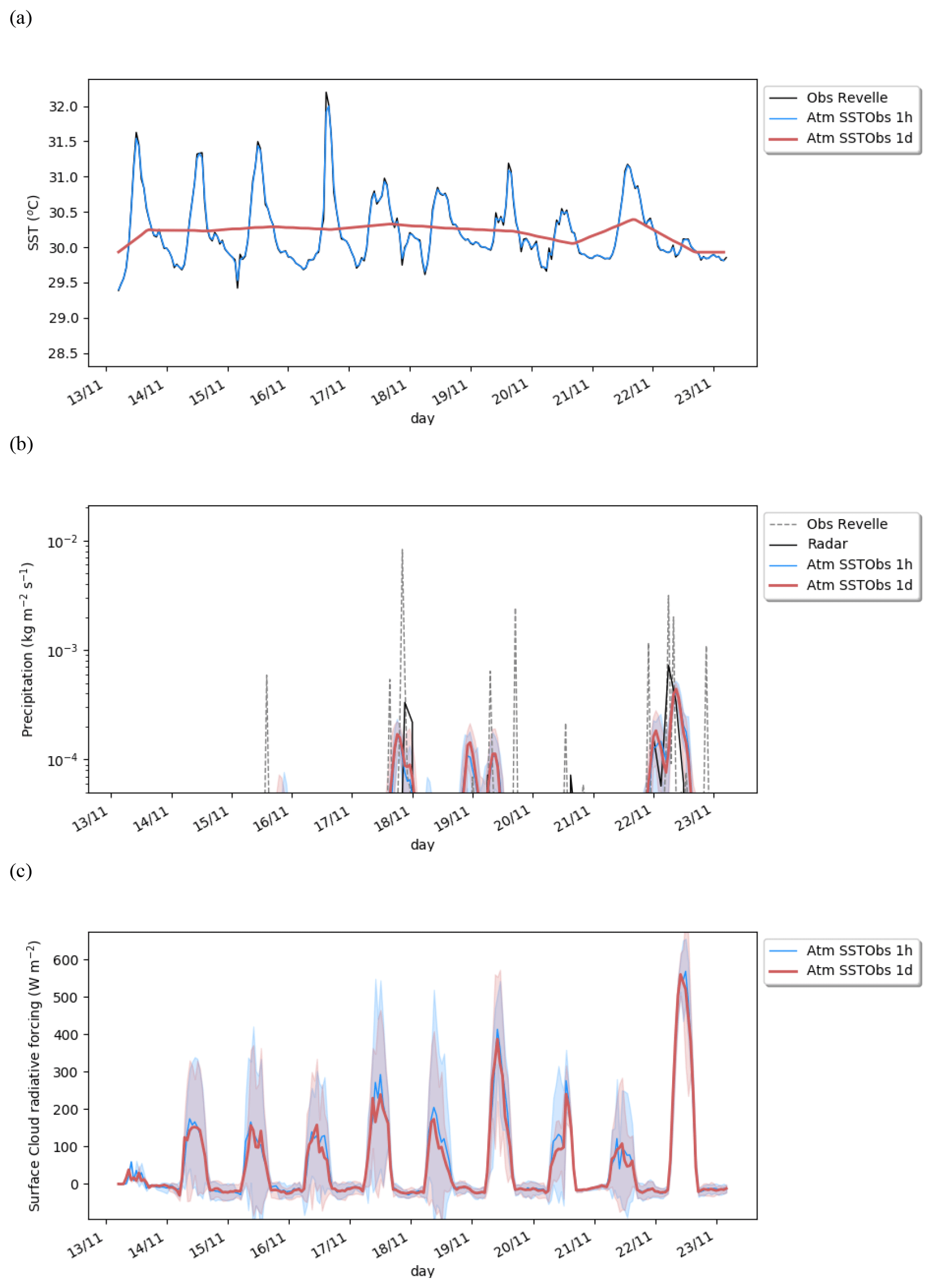
Figure 4 Hourly time series of (a) temperature (^∘C), (b) precipitation (kg m⁻² s⁻¹), and (c) surface cloud radiative forcing (W m⁻²) in atmospheric forced experiments and observed estimates. The shading represents the spread of the member ensemble given by 2 standard deviations.

The surface flux estimations based on either the EC or ID methods are rather noisy and it is difficult to detect a diurnal cycle in the raw time series; even averaged over the 10 d, the mean diurnal cycle is rather noisy (Fig. 6b–c). The standard deviation of the mean diurnal cycle is 43 W m⁻² on average for the latent heat flux and 10 W m⁻² for the sensible heat flux, which is a similar amplitude as the respective mean diurnal range (66 W m⁻² for the latent heat flux and 14 W m⁻² for the sensible heat flux). Indeed, Marion (2014) raises the point that these flux estimates are not accurate under the weak wind conditions of this period. Nevertheless, this dataset provides an idea of the amplitude and phasing of the diurnal turbulent flux cycle.

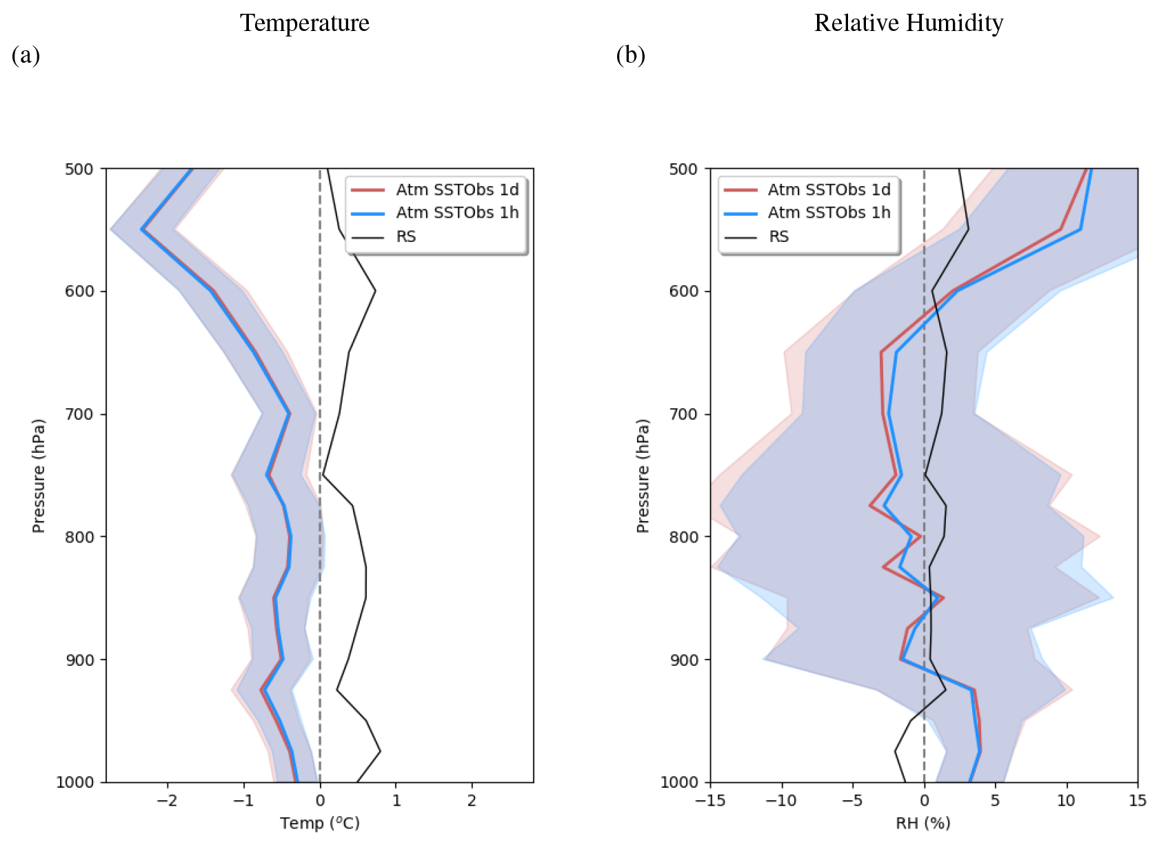
Figure 5 Mean difference in the vertical profile of (a) temperature (^∘C) and (b) relative humidity (%) between atmospheric experiments and the Era-Interim reanalysis (Dee et al., 2011) averaged over the simulated period (13–22 November). The shading represents 2 standard deviations of the inter-member ensemble. The black line indicates the difference between the local sounding data from R/V Revelle and the ERA-Interim reanalysis over the same period.

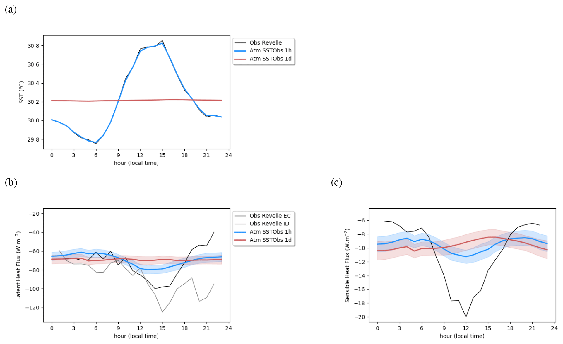
Figure 6 Mean daily cycle of (a) surface temperature (^∘C), (b) surface latent heat flux (W m⁻²), and (c) surface sensible heat flux (W m⁻²) averaged over the simulated period (13–22 November) for the atmospheric experiments and observed estimates. The shading represents 2 standard deviations of the inter-member ensemble.

4.2 In the atmosphere

In an atmospheric model, the SST is a forcing, and thus the representation of the SST diurnal cycle is generally conditioned by the frequency of the product used as a forcing. Here in the reference atmospheric experiment (Atm SSTObs 1h), the forcing is taken from hourly SST observations from the R/V Revelle (Fig. 4a). In this experiment, the model simulates several episodes of precipitation from 18 November 2011, which are concomitant to the local precipitating events occurring at the location of the R/V Revelle, albeit with lower amounts. Such a difference is consistent given the different spatial scales considered, with the model being representative of a region (50 km) larger than that associated with the local precipitation measurements. The amplitude and duration of the simulated events are more similar to the radar observations, which sample the wider area. The cloud radiative effect at the surface has a pronounced diurnal cycle but varies a lot among the ensemble members (Fig. 4c). The cloud amount and radiative properties are thus weakly constrained in this case study, which prevented us from finding any robust differences between our simulations. The mean latent heat flux (70 W m⁻²) and the mean sensible heat flux (10 W m⁻²) are also weaker than observed estimates (88 and 11 W m⁻², respectively). Even if observed values are rather uncertain, this underestimation can also be attributed to an underestimation of the mean wind amplitude simulated (1.5 m s⁻¹ with a standard deviation of 0.7 m s⁻¹), which is much weaker than the observed mean that reaches 2.1 m s⁻¹ with a standard deviation of 1.2 m s⁻¹. Again, as the atmospheric winds are nudged towards the CVA, and this probably highlights the larger spatial scale of atmospheric simulations compared to the local flux measurements. This implies that atmospheric simulations are not fully comparable to local observations given that they are representative of a different spatial scale. To take this different scale into account, mean vertical profiles of temperature and relative humidity are compared to both the Era-Interim reanalysis (Fig. 5, Dee et al., 2011) and the local radio-sounding measurements. It shows that the model is biased cold compared to both the reanalysis and local observations, whereas the relative humidity bias is relatively weak and comparable to the difference between the local soundings and the reanalysis except near the surface where the model is significantly moister than the two references.

To assess the effect of forcing the diurnal SST cycle, we have performed a companion experiment using daily averaged observed SST (Atm SSTObs 1d). The impact of canceling the SST diurnal cycle on the mean surface heat flux is very weak: the sensible heat flux is not impacted, the upward longwave heat flux is only slightly decreased by less than 0.1 W m⁻², and the latent heat flux is decreased by 0.5 W m⁻² (not shown). Similarly, the simulated impact on precipitation and surface cloud radiative effect is weak but within the ensemble range (Fig. 4b–c); the mean impact on the atmospheric mean temperature and relative humidity profiles (Fig. 5) is also negligible. Even if the mean state is not changed, the inclusion of an SST diurnal cycle may impact the diurnal cycle of the surface heat fluxes and of the atmospheric profiles. We mainly observe an impact on the turbulent heat flux diurnal cycle: the latent heat flux diurnal cycle decreases (in absolute value) by more than 16 W m⁻², whereas the sensible heat flux amplitude is only reduced by 1 W m⁻². The latent heat flux daily maximum is better phased when forcing with hourly SSTs. The impact on the tropospheric temperature and relative humidity mean diurnal cycles is shown in Fig. 7. The impact on specific humidity in the afternoon is similar to that on relative humidity (not shown). The surface temperature cooling at night and warming in daytime are limited to near-surface layers below 925 hPa. Similarly, we observe a near-surface drying during daytime and a moistening at nighttime. Further analysis of the simulated profiles during the afternoon indicates a slightly deeper and more active boundary layer, consistent with its increased destabilization by warmer SSTs at that time (not shown). The effect, however, remains weak and weakly significant. There is no clear significant impact above 925 hPa. In this 1D setup, the SST diurnal cycle does not imprint on the mid-troposphere or on the precipitation. It is likely that the large-scale forcing largely limits any feedback from the surface in this 1D configuration.

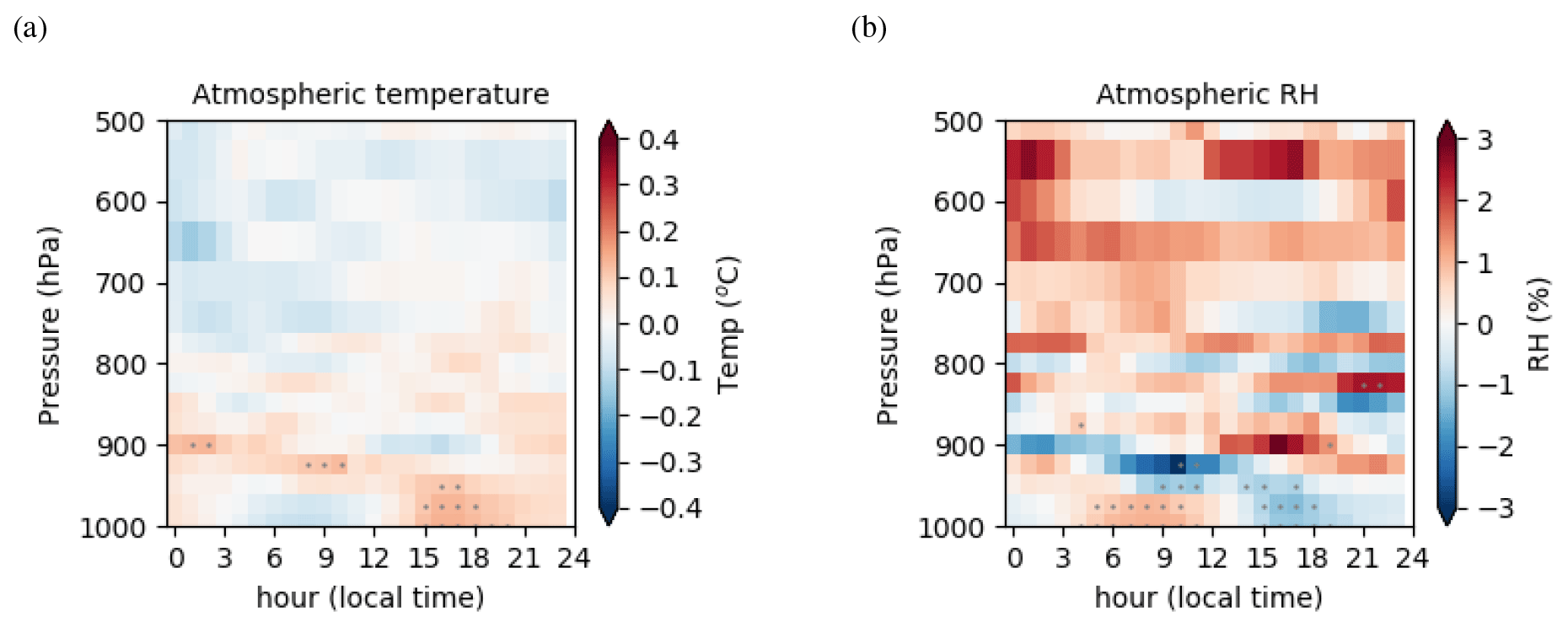
Figure 7 Change in mean daily cycle between the experiment with hourly SST forcing (Atm SSTObs 1h) and the experiment with daily SST forcing (Atm SSTObs 1d) for (a) the atmospheric temperature (^∘C) and (b) relative humidity (%). Dots indicate significant anomalies according to a Student's t test at the 95 % significance level.

4.3 In the ocean

In contrast to the atmosphere-only configuration, in the ocean-only configuration the SST is prognostic. The SST evolves according to the heat budget of the oceanic top layer, and it is thus representative of the first layer. The SST thus represents 1 m depth-averaged temperature in the reference configuration. We may wonder if the simulated SST would better match the observed skin SST if the model resolution was increased near the surface. Also, the role of vertical discretization has been raised in many studies (Bernie et al., 2005; Hsu et al., 2019; Ge et al., 2017), but these studies generally test resolution between 1 and 10 m. Hsu et al. (2019) assess the diurnal SST representation in the ACCESS-S1 model, which also uses NEMO at a 1 m vertical resolution. They suggest that flaws in representing the diurnal warming may be due to insufficient vertical resolution or deficiencies in vertical mixing in the NEMO model.

The column model allows us to tackle this question relatively easily. We thus extend the analysis already made in Bernie et al. (2005) to higher vertical resolution. The way the vertical coordinate is defined in CNRM-CM6-1 (ln zco case in Madec et al., 2017) makes it complicated to change the ocean vertical resolution (as also raised in Hsu et al., 2019). To ease the change in vertical grid scale, we have moved to a uniform grid representation and limited the depth to 135 m. To check the effect of changing the vertical grid formulation and reducing the ocean depth, we first perform an experiment in which the vertical resolution is set uniformly to 1 m (ocean v1m) as in the first layer of the reference experiment. Then we have increased the vertical resolution to 1 cm (ocean v1cm) and reduced it to 10 m (ocean v10m).

The results from these simulations are compared to the reference experiment in Fig. 8. We verified that the uniform vertical discretization with 1 m resolution behaves similarly as in the control simulation that used a more complex discretization but a similar resolution near the surface. As already shown in former studies, a coarser vertical resolution of 10 m strongly reduces the DTR to 0.3 ^∘C. With a 1 m resolution, the mean DTR is 1.0 ^∘C; this is only slightly less than the 1.1 ^∘C obtained with 1 cm resolution, which is close to the observed estimate. Also note that increasing the resolution has a small impact on the timing of the maximum, which is advanced by 1 h.

Figure 8 Mean daily cycle of surface temperature (^∘C) for the reference ocean forced experiment (orange) and sensitivity tests to the ocean vertical discretization (green).

To get a more quantitative assessment of the DTR representation depending on vertical resolution, Fig. 9 provides the percentage of the observed DTR amplitude simulated by the OSCM for a large set of vertical resolution values (blue dots, between 1 cm and 10 m). Between 1 and 10 m, this study confirms the Bernie et al. (2005) findings (their Fig. 10) with a rapid decrease in simulated SST amplitude with decreasing resolution. With resolutions coarser than 4 m, the ratio of SST amplitude drops below 50 %. In contrast, when resolution gets thinner than 1 m the increase in DTR is rather small. The grey line represents the DTR obtained in the 1 cm resolution simulation but averaging the temperature over the corresponding depth. The amplitude of the DTR representation corresponds well to that of the corresponding resolution experiment, meaning that when running coarse vertical grid resolution, the lowest DTR obtained is due to the fact that it represents a larger “bulk” and not a flaw in the existing subgrid ocean process representation. If we compare the DTR obtained at 5 m depth in the 1 cm resolution experiment with the DTR measured by the thermosalinograph at the same depth, the amplitude of the DTR simulated is about half of the observed DTR (not shown). This suggests that the diurnal processes are concentrated in a shallower layer than in observations. This also tends to show that improving the representation of the nighttime cooling necessitates better representing the processes involved (Moulin et al., 2018). To go a step further, we would need accurate observations of the DTR as a function of depth, which are difficult to measure accurately and which were not available at the position of the R/V Revelle for the present case (Matthews et al., 2014).

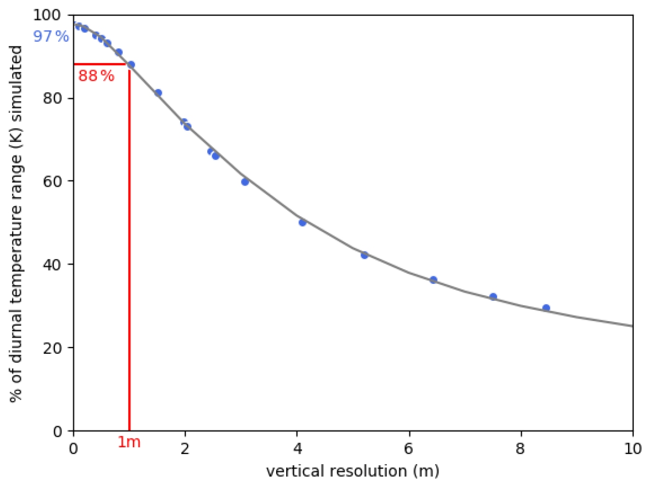
Figure 9 Ratio (%) of the simulated diurnal SST range to the observed range at the location of the R/V Revelle averaged over the first 5 d of the case study depending on the vertical resolution in the ocean model (blue dots). The grey line represents the ratio estimated from the experiment with the finest vertical resolution (i.e., 1 cm) by averaging the temperature over the corresponding depth, with the blue value being the ratio at the first depth in this simulation. Note that the statistics could not be computed over the 10 d of the experiments since some vertical resolution experiments were instable after these first 5 d.

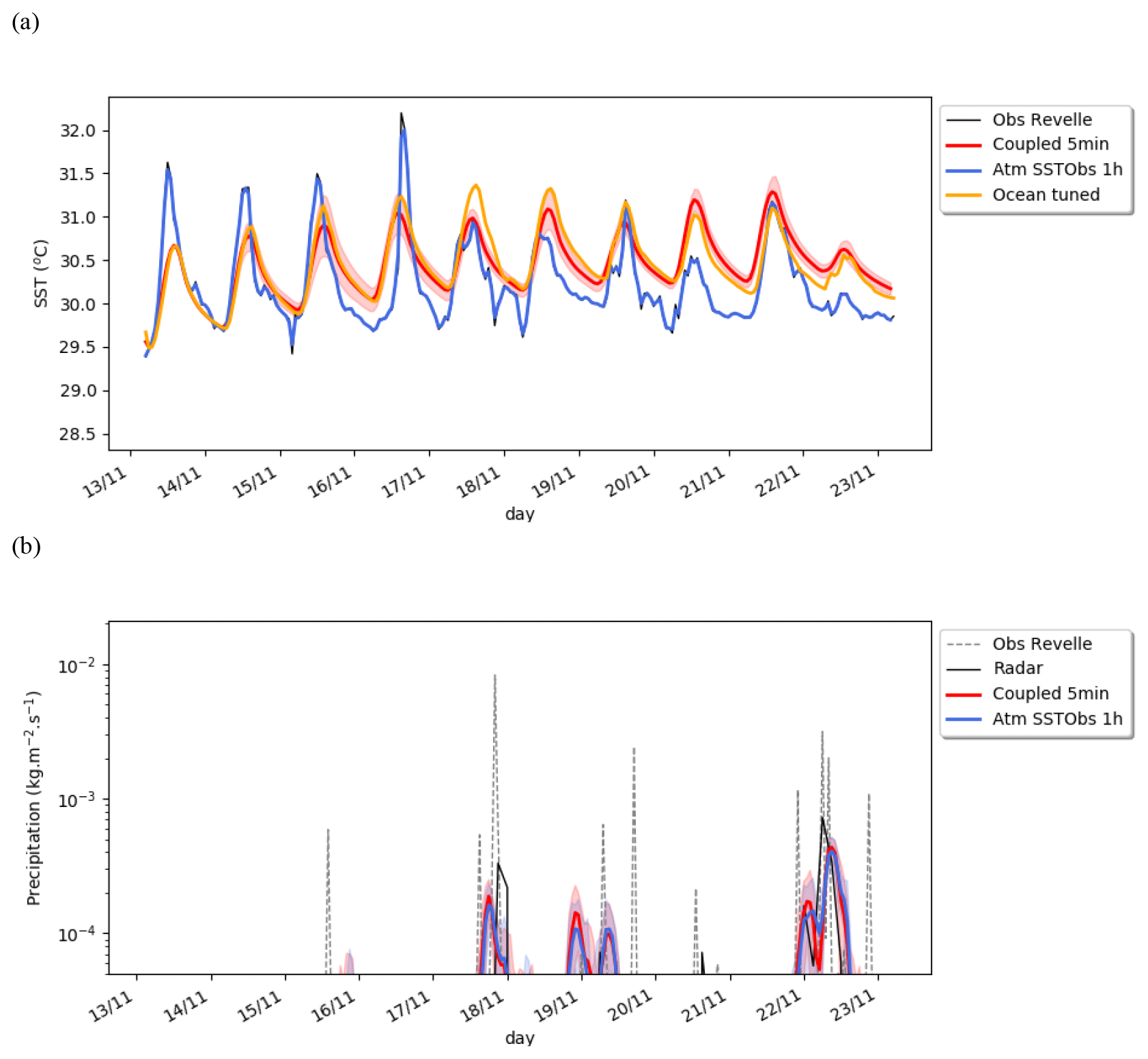
Figure 10 Hourly time series of (a) surface temperature (^∘C) for the coupled experiment (in red), the reference atmospheric (blue) and ocean forced (orange) experiments along with observations at the position of the R/V Revelle (black), and (b) precipitation (kg m⁻² s⁻¹) for the coupled (in red) and the reference atmospheric (blue) experiments along with local observations at the position of the R/V Revelle (dashed grey) and radar estimates (black). The shading represents 2 standard deviations of the inter-member ensemble.

This sensitivity test shows that using a 1 m vertical resolution in an ocean model is a good compromise in state-of-the-art models. Even with nonuniform vertical coordinate discretization, reaching a 1 cm resolution near the surface would be numerically unfeasible in global 3D climate models. In such models, the near-surface effect could be introduced well by using or adapting warm-layer parameterizations (Zeng and Beljaars, 2005; Bellenger et al., 2017; Gentemann et al., 2009; Scanlon et al., 2013) as proposed in Yang et al. (2017).

5 SST diurnal cycle in coupled configuration

5.1 Impact of the coupling

The coupled reference experiment is based on the stand-alone configurations discussed in the previous section with the “ocean tuned” setup for the ocean component. In the reference coupled experiment, the coupling time step is set to 5 min to compare the effect of the coupling in the coupled configuration wherein the asynchronicity is the lowest. The effect of increasing the coupling time step will be discussed in the next section.

Figure 10a shows the SST evolution for the coupled reference experiment along with reference uncoupled experiments and R/V Revelle observed SSTs. The coupled model SST shows a clear diurnal cycle and closely follows the behavior of the uncoupled ocean experiment (ocean tuned) with a similar warming trend. The simulated SST has a warm bias (+0.2 ^∘C) of similar amplitude as that in the ocean forced case (+0.2 ^∘C). The warming trend probably results from a lack of nighttime mixing in the case of strong upper-ocean stratification as shown in Brilouet et al. (2021).

In the model, the intensity of the diurnal cycle does not change much during the period unlike in observations. During the first 4 d, the DTR is underestimated in both ocean forced and coupled simulations. This suggests that the weaker DTR results mainly from flaws in the ocean model, which is probably too diffusive. As mentioned before, more work would be needed to improve the realism of the ocean simulation in this case study. Compared to ocean forced simulations, the DTR tends to be reduced in coupled simulations, but the reduction is in the range of coupled simulation spread. As the spread is largely associated with cloud variability, the subsequent reduction in DTR in coupled mode may be due to differences in cloud radiative forcing between observations and simulations. Similarly, the model simulates precipitation events (Fig. 10b), but they do not seem to be associated with a reduction in DTR as in observations. There are several factors that could explain this weak impact: the simulated precipitation events may be too weak to impact the surface turbulent fluxes, which could alter the SST diurnal cycle, or there may be missing processes in the model that should impact the surface turbulent fluxes. For instance, convective precipitation is usually associated with gusts that are known to increase the turbulent fluxes (Godfrey and Beljaars, 1991); such a gustiness effect is not included in the CNRM-CM6-1 model and may explains this weak impact of precipitation events on DTR.

The simulated precipitation is similar between the coupled and the atmosphere-only configurations (Fig. 10b). The SST diurnal cycle shape (Fig. 11a) also looks like the one of the ocean-only simulation, with the mean DTR being only slightly reduced to 0.9 ^∘C. The latent heat flux mean daily cycle is very similar to the one simulated by the atmosphere-only simulation (Fig. 11b). The most striking feature is the large discrepancy between the mean latent heat flux estimated in the ocean forced simulations compared to the atmospheric and coupled simulations. This difference is explained well by the surface ocean forcing used: the ocean-only experiment is forced by the R/V Revelle's local observations, whereas the coupled experiment interactively computes variables and fluxes at the air–sea interface. In particular, we have shown in Sect. 4.2 that the wind forcing explains such a difference. In the ocean, the difference in turbulent heat flux between the forced and coupled experiment does not impact the simulated SST much, and it clearly reflects the fact that the ocean vertical profiles of temperature and salinity are only weakly impacted by the coupling and the change in surface turbulent fluxes.

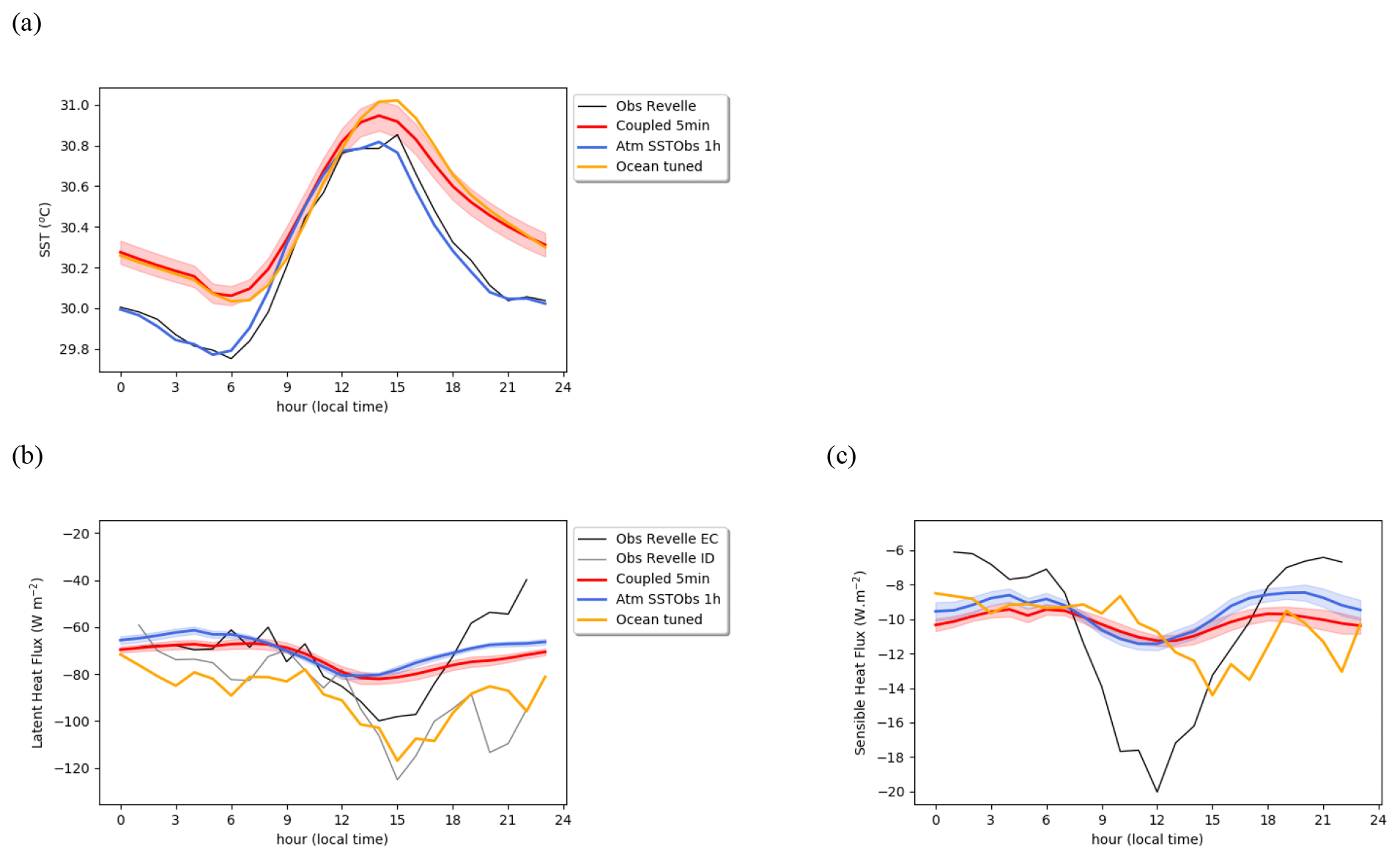
Figure 11 Mean daily cycle of (a) surface temperature (^∘C), (b) surface latent heat flux (W m⁻²), and (c) surface sensible heat flux (W m⁻²) averaged over the simulated period (13–22 November) for the coupled experiment (in red) and reference atmospheric (blue) and ocean forced (orange) experiments along with observations at the position of the R/V Revelle (black). The shading represents 2 standard deviations of the inter-member ensemble.

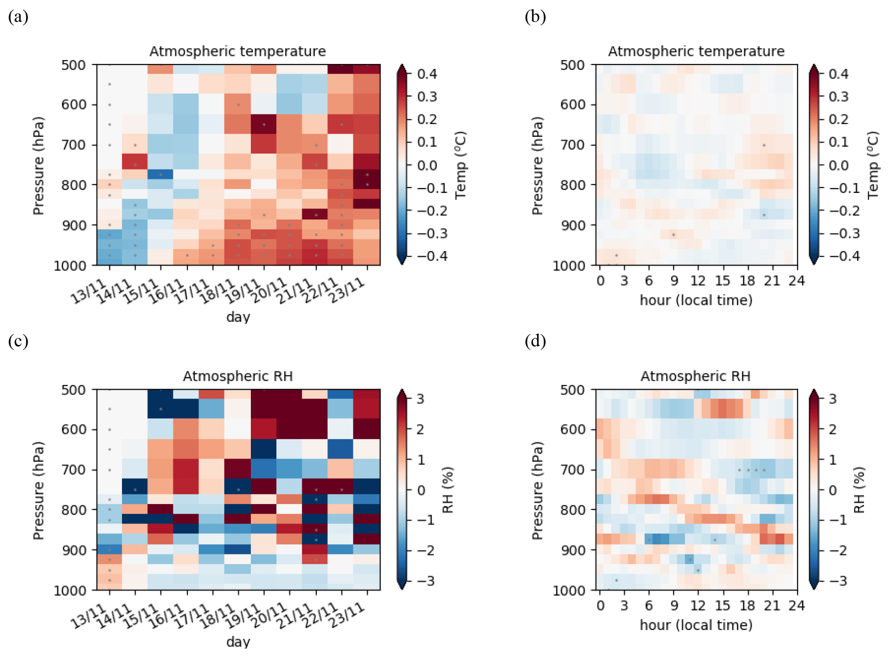
Figure 12 Change in mean daily vertical profile of (a) temperature (^∘C) and (c) relative humidity (%) between the reference coupled experiment and the Atm SSTObs 1h experiment. (b, d) The respective change in the mean diurnal cycle averaged over the 10 d period with the mean bias removed at each level. Dots indicate significant differences according to a Student's t test at 95 % the confidence level.

Figure 12a shows the evolution of the difference in the daily mean atmospheric vertical profile of temperature between the coupled experiment and the atmosphere forced experiment. After the first 2 d, a warm anomaly develops near the surface and progressively extends up to the lower free troposphere by the end of the 10 d period. This shows the impact of the surface warm anomaly on the atmospheric column. There are much less significant impacts on the relative humidity daily mean profile (Fig. 12c). Having removed the mean biases, the impact of the coupling on the atmospheric diurnal cycle is weak and nonsignificant. To summarize, the first effect of the coupling is a change in the mean state, with a very weak impact on the simulated diurnal cycle. The coupled simulation surface temperature follows the ocean forced experiment temperature evolution, in contrast to the surface turbulent heat fluxes, which mainly follow the atmospheric forced simulation. The latter are more impacted by the change in atmospheric surface wind than by the change in SST.

5.2 Impact of the coupling frequency

Figure 11a emphasizes that in the coupled experiment, the SST daily peak occurs between 12:00 and 15:00 LT relatively in phase with observations, even if there is probably a short delay of less than 1 h. In the reference coupled experiment, the coupling time step is 5 min, which is much less than in state-of-the-art global climate models. In 3D climate models, the individual component time steps are larger than in this single AOSCM configuration and do not allow us to couple at such high frequency. Hsu et al. (2019) show that with a 1 h coupling, they still have deficiencies in the phasing of the SST maximum but could not go far beyond in their AOGCM. Here the AOSCM configuration allows us to tackle this question with more detail. Increasing the coupling frequency from 1 d to higher frequencies has been done in several CMIP6 climate models but with the use of a 3 h coupling time step (Li et al., 2020; Sellar et al., 2020) or a 1 h coupling time step (Danabasoglu et al., 2020; Mauritsen et al., 2019). Tian et al. (2019) and Li et al. (2020) both report an improvement in El Niño–Southern Oscillation (ENSO) representation, especially when switching from a daily to higher coupling frequency. The effect of using a 3 h coupling time step over a 1 h coupling time step, however, is not discussed. The 1D coupled configuration is a relevant tool to highlight the first-order consequences of such a choice. Here, we run a set of experiments in which we only change the coupling frequency, exploring 5 min, 15 min, 1 h, 3 h, and daily coupling time steps.

Figure 13 shows the SST mean daily cycle for these sensitivity experiments. With a daily coupling, unsurprisingly the SST is held constant all day to 30.3 ^∘C. In all other experiments with an infra-daily frequency the mean SST is similar (30.4 ^∘C). This means that the rectification effect raised in Bernie et al. (2005) may be present but limited to 0.1 ^∘C. For a coupling time step between 5 min and 1 h, the DTR is similar (0.9 ^∘C) and drops relatively weakly with the 3 h coupling to 0.8 ^∘C. The main difference between the experiments with an intra-daily frequency comes from the time of maximum SST, which is consistently delayed with the increased coupling period. Indeed, with the asynchronous coupling algorithm used in the model, the ocean model uses the solar heat flux calculated in the atmospheric model over the former coupling time step. Thus, increasing the coupling time step increases the delay by which the ocean model sees the solar radiation diurnal cycle. The daily maximum is reached around 14:00 LT for the 5 min coupling time step, in relative agreement with in situ observations. With a 15 min coupling time step, the maximum is only marginally delayed. With a 1 h coupling time step, there is a delay of 2 h. With a 3 h coupling time step the delay is increased to 6 h.

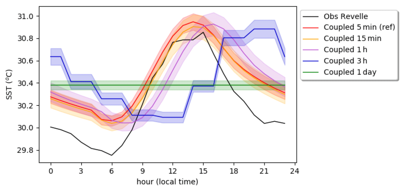
Figure 13 Mean daily cycle of SST (^∘C) in sensitivity experiments to the coupling frequency averaged over the simulated period (13–22 November). The shading represents 2 standard deviations of the inter-member ensemble.

In our coupled model, the rectification effect is relatively weak compared to the estimation of 0.34 ^∘C given in Bernie et al. (2005); however, there are several differences in our study that may explain such a difference in amplitude. We may wonder if the coupling could reduce this rectification effect or if such a rectification effect is less active in the present case study due to different processes at play. To disentangle the coupling effect, we perform additional ocean forced experiments driven by the atmospheric flux obtained in the 1 h coupled experiment (Table 2). A first experiment uses the atmospheric forcing at a 1 h time step (ocean 1 h forcing) and a second one uses the same forcing but after being daily-averaged (ocean daily avg forcing). Figure 14 shows the evolution of the SST and its daily mean in the coupled experiments and in the ocean forced experiments. First, the difference between the 1 h and daily coupled experiments (Fig. 14a) does not increase all along the period as one would expect if the rectification effect was at play. The daily coupled experiment is colder the first 2 d, then reaches the mean temperature of the coupled 1 h experiment and even gets warmer the following 5 d. The first day of colder SST in the 1 d coupled experiment compared to the 1 h coupled experiment seems attributable to a longer time needed to adapt to the atmospheric warming due to the “weak coupling” induced by the fact that the ocean receives the new atmospheric state with a 1 d delay. It does not show a clear rectification effect. In the ocean forced experiment, the behavior is closer to what was shown in Bernie et al. (2005), with the daily forcing experiment being colder by 0.2 ^∘C than the hourly forced experiment the first 9 d of the period. Also note that the difference reverses quickly when the amplitude of the diurnal cycle weakens at the end of the period. The surface heat flux differences between the two coupled experiments mainly emerge from the asynchronicity introduced by the coupling. When the ocean and atmosphere components are coupled at the daily timescale, the ocean receives the atmospheric surface fluxes computed as the average over the previous day. In contrast, the hourly coupling introduces a delay of only 1 h. In our experiments, the asynchronicity effect is much larger than a possible rectification effect (not shown). Thus, although the ocean–atmosphere single-column model appears to be a valuable tool to investigate further the rectification effect in a coupled framework, a further step needs to be achieved to change the time coupling algorithm and thereby be able to investigate the rectification effect properly. Our study tends to show that the rectification effect is weaker than expected in the ocean forced experiments and remains to be shown in coupled mode.

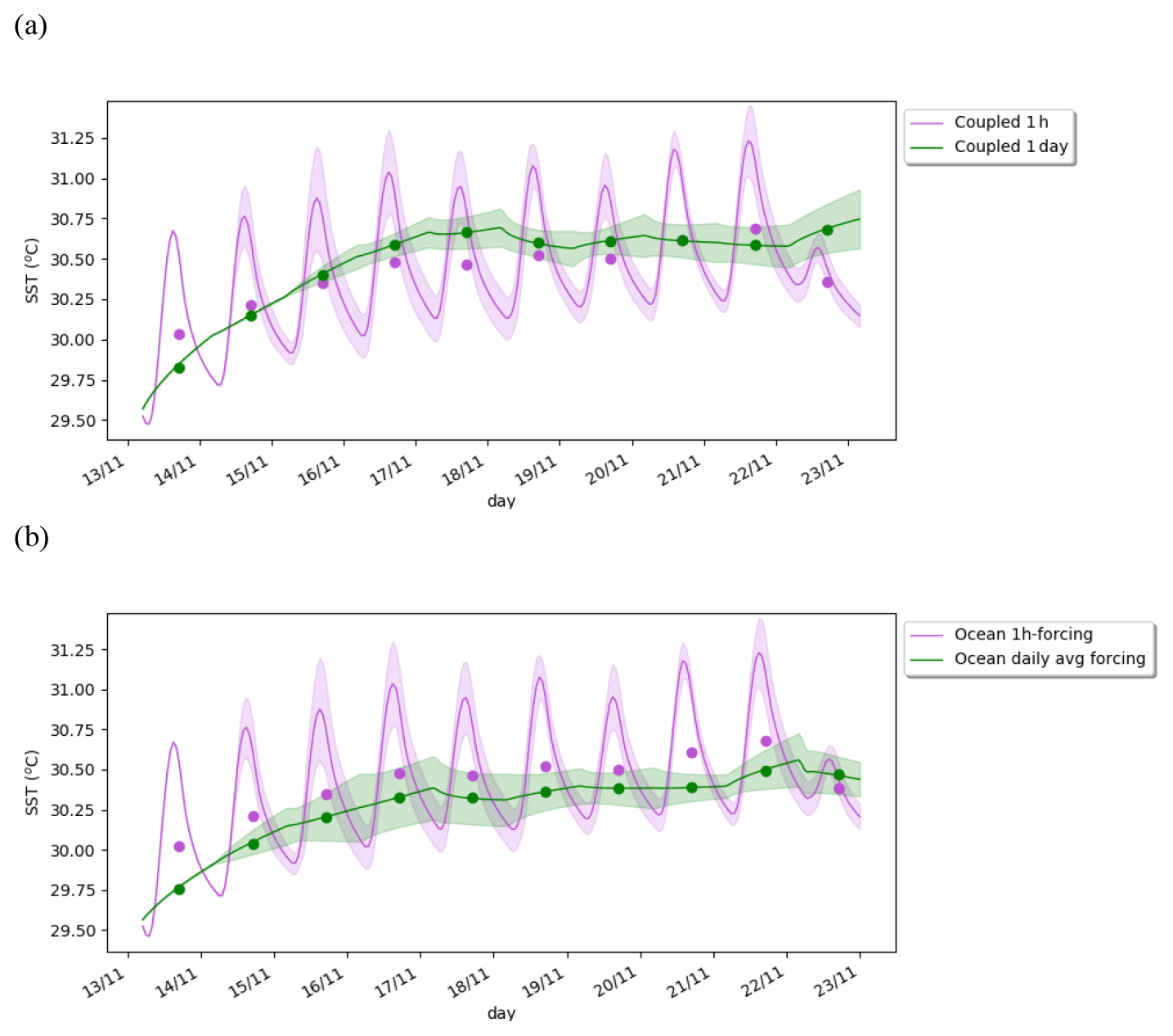
Figure 14 Evolution of SST (^∘C) simulated by the ocean component for (a) the hourly and daily coupled experiments as well as the (b) ocean forced experiments forced with the hourly coupled atmospheric state taken hourly or as a daily average. The dots indicate the daily mean SST values for each experiment.

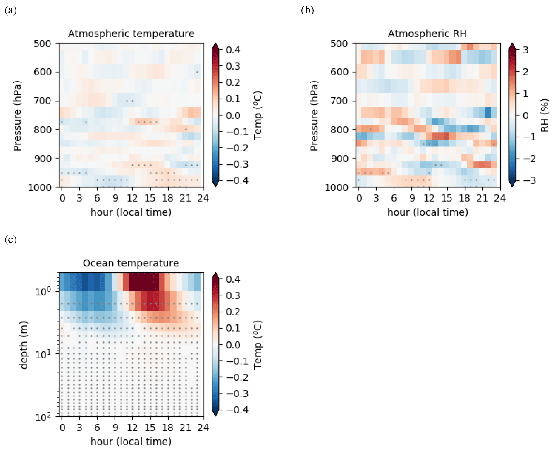
Figure 15 Change in mean diurnal cycle with the mean bias removed at each level (right column) between the 5 min coupled experiment and the 1 d coupled experiment for (a) the atmospheric temperature (^∘C), (b) the relative humidity (%), and (c) the ocean temperature (^∘C). Dots indicate significant differences according to a Student's t test at the 95 % confidence level.

Figure 15a–b show the impact of introducing the SST diurnal cycle in the atmospheric column in coupled mode to compare with the results in atmospheric forced mode (Fig. 7). The effect of high-frequency coupling compared to daily coupling is qualitatively similar, with impacts limited to the near-surface atmospheric layers. The intensity of the signal is consistently weaker with the underestimated DTR in the coupled simulation. We also observe an impact on the diurnal evolution of oceanic temperature in near-surface layers (Fig. 15c). The daily warming of the ocean upper layers starts from 10:00 LT, which is several hours earlier than in the first atmospheric layers. This shows that the ocean surface temperature warms due to increasing solar radiative heat flux and that the surface temperature warming then feeds back on the atmosphere afterwards.

Figure 16 illustrates the impact of changing the coupling frequency from 5 min to 1 h (3 h) on ocean and atmospheric columns. This can be viewed as the error made when the coupling time step is fixed to 1 h (3 h) as in 3D models, since with a 5 min time step we have shown that the SST diurnal cycle matches the observed one well. As expected, the impacts are larger for the 3 h frequency than for the 1 h frequency. In both cases, they are limited to the lower troposphere. The impact can be regarded as a delay of the diurnal cycle, with reduced ocean temperature between 08:00 and 15:00 LT and increased the rest of the day.

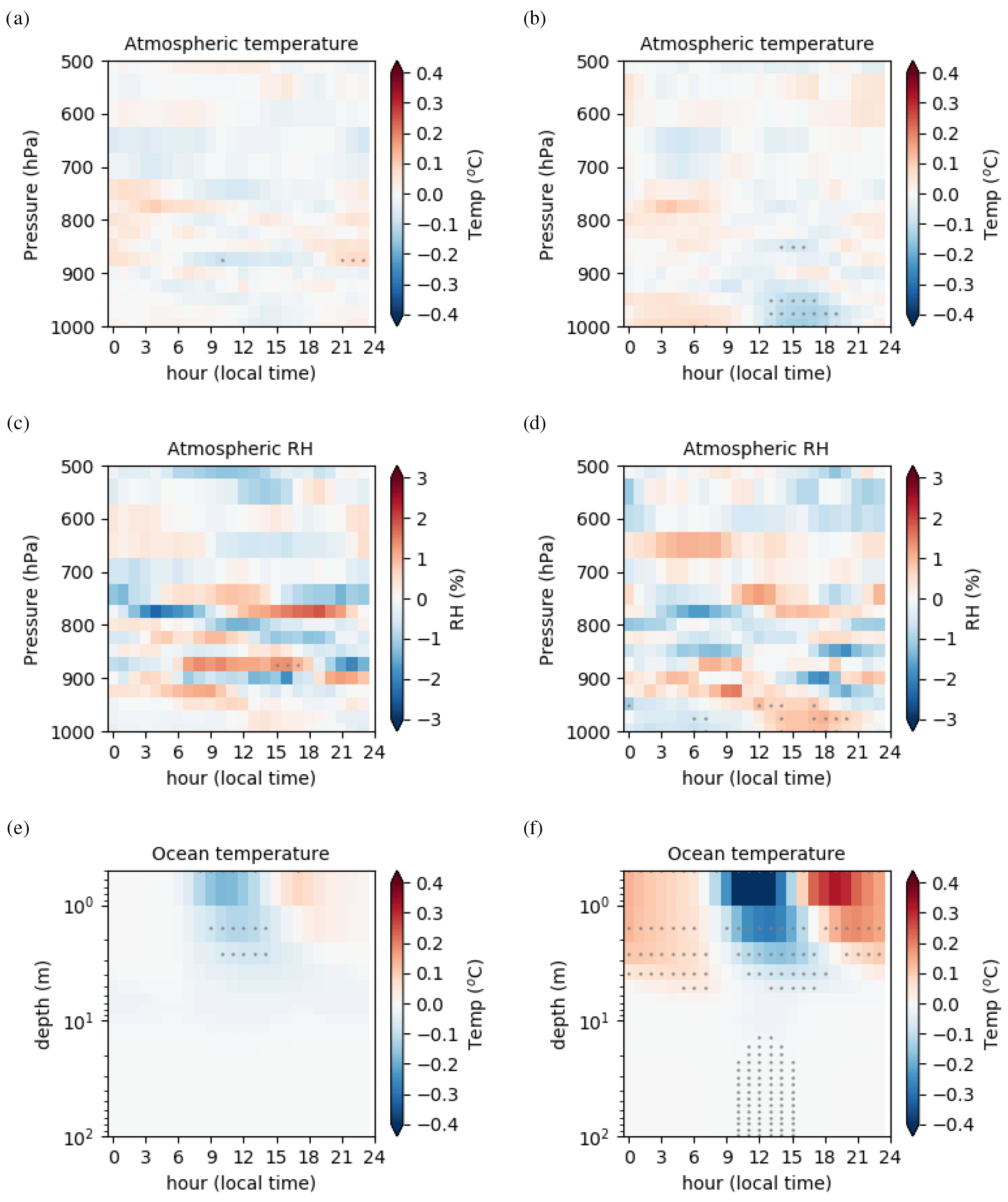
Figure 16 Change in mean daily cycle between the 1 h coupling experiment and the 5 min coupled experiment (left) and between the 3 h coupling experiment and the 5 min experiment (right) for (a, b) the atmospheric temperature (^∘C), (c, d) the relative humidity (%), and (e, f) the ocean temperature (^∘C). Dots indicate significant differences according to a Student's t test at the 95 % confidence level.

We could expect that the phase change in the daily cycle of the atmospheric temperature could impact the cloud cover daily cycle, but given the very large spread in cloud radiative forcing in between members, it has not been possible to detect a robust impact (consistent with the weak impact seen on relative humidity).

To summarize, from the ocean point of view, the coupling has a very weak impact on the simulated SSTs. The rectification effect shown in Bernie et al. (2005), which is present in ocean forced mode, disappears when coupling with the atmospheric model. From the atmospheric point of view, the effect of the coupling can be decomposed into two effects. First, the coupling leads to a mean state change, with the SST in coupled mode being biased as in the ocean forced experiment. The mean state change is relatively similar for all coupling time steps. The second effect is linked to the sub-daily SST variability itself. This second effect has been assessed in both atmospheric forced mode (Fig. 7) and ocean–atmosphere coupled mode (Fig. 15). The effect of the SST diurnal cycle is very similar and limited to the atmospheric boundary layer below 900 hPa in both configurations on the atmospheric temperature and relative humidity, with the signal being weaker in coupled mode.

6 Discussion and conclusion

To ease the CNRM-CM model development, we derive from the full 3D coupled GCM an atmosphere–ocean single-column version called CNRM-CM6-1D. This configuration consists of coupling the already existing column versions of the atmospheric and ocean models used in CNRM-CM. The 1D model coupling closely follows the global model coupling setup, enabling the study of the coupling between the ocean and atmosphere as in the 3D model but in a more constrained framework. Running such a model can be done on a common personal computer in a few minutes. Thus, it is possible to perform numerous tests that ease debugging and allow one to run many sensitivity tests. Such a configuration is fully relevant to investigate in detail some of the feedbacks between individual components or between parameterizations. When developing new parameterizations, it is also much easier to implement and test them in this 1D configuration.

As a first step, we illustrate here the use of this model to discuss the necessary elements to be included in 3D climate models to properly represent the sea surface temperature diurnal cycle. To this aim, the 1D configuration has been implemented for a CINDY2011/DYNAMO case study. This case study is particularly relevant since we observe large SST diurnal variations during the period. A specific large-scale atmospheric forcing representative of a 50 km radius around the R/V Revelle is used to focus on the local scale.

For the ocean, there is no specific large-scale forcing available and it is not straightforward to derive such a forcing. In its standard configuration, the model overestimates the upper-ocean stability and the surface warming. This strong stability is not reduced by imposing a negative trend in temperature mimicking a missing large-scale advective forcing. We therefore increase the background eddy diffusivity to artificially enhance the unresolved turbulent mixing. This results in a better match with the observed ocean stability profiles and a more realistic DTR. We do not conclude from this that the background eddy diffusivity should be changed in the 3D model, as a deeper analysis over a wider variety of cases is required. In particular, the wind forcing observed at the location of the R/V Revelle during the CINDY2011/DYNAMO campaign is relatively weak and does not span the variability observed or simulated in the 3D model. This result points, however, to the need for an improved representation of near-surface mixing processes in ocean models, especially under stable conditions. This highlights the fact that such a 1D configuration is a relevant tool to investigate the parameterization of ocean mixing processes.

In this case study, it has been possible to run the model for periods longer than 10 d without imposing a large-scale ocean circulation. However, it should be highlighted that this is probably not the case everywhere in the ocean, and thus the use of this model for other case studies would require getting such a large-scale ocean forcing. It should be stressed, though, that the neglect of large-scale circulation is a common practice for single-column ocean modeling experiments (e.g., Reffray et al., 2015, and references therein).

The case study used here is particularly relevant to study processes related to the SST diurnal cycle. In an atmospheric forced model, the SST is a forcing and the capability of representing its diurnal cycle mainly depends on the availability of such datasets. The impacts of including the SST diurnal cycle are relatively weak but could be larger in a less constrained modeling framework. To take them into account, it could be valuable to implement a parameterization of the diurnal warm layer (Gentemann et al., 2009; Scanlon et al., 2013; Bellenger et al., 2017; Yang et al., 2017). Such an implementation could be easily validated based on this 1D case study. Such a parameterization could also be used in coupled configurations: with 1 m ocean vertical resolution the simulated DTR captures 90 % of the observed estimate, and therefore a warm-layer parameterization may help improve the DTR amplitude.

The pure effect of representing the SST diurnal cycle in atmospheric forced and coupled simulations is similar and limited to the near-surface layers in both the atmosphere and the ocean. We could have expected to find an impact of the SST diurnal cycle on convection as found in Zhao and Nasuno (2020), but it was not the case here. We may hypothesize that, in the present 1D setup, the convection is mostly constrained by the large-scale forcing and that surface temperature would impact convection through changes in vertical motion that are not interactive here.

In our 1D configuration, the impact of coupling on the ocean is very weak, as pictured by the similar evolution of SSTs. Additionally, the “rectification” effect highlighted in Bernie et al. (2005) due to the representation of the diurnal temperature evolution is not present in the coupled experiments. As a result, in the atmosphere, the impact of coupling is nearly directly the sum of the impact of changing the mean state in SST as in the ocean forced simulation plus the effect of introducing the diurnal SST cycle, without any coupled feedbacks. This is probably due to the absence of feedbacks arising from the large-scale dynamics. Such a configuration is of great value to assess new developments and disentangle their first-order impacts, but it remains a simplified approach to be complemented by 3D studies.

Generally, in 3D simulations, atmosphere-only simulations are done using low-frequency varying SSTs, and thus when we compare an atmosphere forced experiment to a coupled experiment, the effect of introducing an infra-daily varying SST and the pure coupling effect are both introduced without being clearly assessed separately. In the 1D column configuration it is easy to disentangle these two effects, and this should be better highlighted in studies with full GCMs.

In 3D models, reducing the coupling time step can be expensive in terms of computational cost, and it is generally set to 1 h or 3 h. Thanks to the 1D configuration, we have been able to assess the effect of such choices. The effect of changing the coupling period is to delay the timing of the daily maximum SST without impacting the DTR. We have shown that with a 5 min or 15 min coupling time step the models simulate the timing of the daily maximum SST well. With a 1 h coupling time step the delay is limited to 2 h, and with a 3 h coupling time step, the delay extends to 5 h, which becomes important relative to the day length.

Such 1D coupled configurations are particularly relevant to perform studies related to time coupling schemes. It is a very practical tool to test new approaches like Schwartz methods that enable correcting the mismatch between components due to asynchronous coupling through an iterative method (Marti et al., 2021) and to assess the effect of different coupling algorithms from purely sequential to asynchronous. Using a Schwartz algorithm for coupling would enable properly assessing the rectification effect in coupled mode. It is also an interesting tool to assess the effect of surface flux parameterizations on both ocean and atmospheric boundary layers.

More generally, to be useful for the development and evaluation of surface flux and boundary layer parameterizations and more generally for modeling choices related to the vertical physics, there is a need to get several coupled 1D case studies as is done for the atmosphere 1D case studies. Following an initiative from the DEPHY program (http://www.umr-cnrm.fr/dephy/, last access: 18 April 2022), the community is currently developing common standards for ASCM input forcing in order to facilitate sharing and implementation of the wide library of currently available ASCM cases. A similar effort would clearly benefit future AOSCM case studies.