the Creative Commons Attribution 4.0 License.
the Creative Commons Attribution 4.0 License.
 | 19 Apr 2022
CondiDiag1.0: a flexible online diagnostic tool for conditional sampling and budget analysis in the E3SM atmosphere model (EAM)
Kai Zhang
Philip J. Rasch
Vincent E. Larson
Xubin Zeng
Shixuan Zhang
Ross Dixon
Numerical models used in weather and climate prediction take into account a comprehensive set of atmospheric processes (i.e., phenomena) such as the resolved and unresolved fluid dynamics, radiative transfer, cloud and aerosol life cycles, and mass or energy exchanges with the Earth's surface. In order to identify model deficiencies and improve predictive skills, it is important to obtain process-level understanding of the interactions between different processes. Conditional sampling and budget analysis are powerful tools for process-oriented model evaluation, but they often require tedious ad hoc coding and large amounts of instantaneous model output, resulting in inefficient use of human and computing resources. This paper presents an online diagnostic tool that addresses this challenge by monitoring model variables in a generic manner as they evolve within the time integration cycle.
The tool is convenient to use. It allows users to select sampling conditions and specify monitored variables at run time. Both the evolving values of the model variables and their increments caused by different atmospheric processes can be monitored and archived. Online calculation of vertical integrals is also supported. Multiple sampling conditions can be monitored in a single simulation in combination with unconditional sampling. The paper explains in detail the design and implementation of the tool in the Energy Exascale Earth System Model (E3SM) version 1. The usage is demonstrated through three examples: a global budget analysis of dust aerosol mass concentration, a composite analysis of sea salt emission and its dependency on surface wind speed, and a conditionally sampled relative humidity budget. The tool is expected to be easily portable to closely related atmospheric models that use the same or similar data structures and time integration methods.
- Article
(6746 KB) - Full-text XML
- BibTeX
- EndNote


Atmospheric general circulation models (AGCMs) used in climate research and weather prediction are simplified mathematical representations of the complex physical and chemical processes (phenomena) driving the evolution of the Earth's atmosphere. Despite the necessity of simplification due to the limitation in computing resources, it is highly desirable that, to the extent possible and practical, models should be based on first principles and robust quantitative relationships in atmospheric physics and chemistry so that the same models can reliably provide good accuracy under historically observed atmospheric conditions as well as in the climate of the future.
Many tools have been used for assessing the behavior and fidelity of the atmospheric processes represented in numerical models. Among those, budget analyses are a useful method for quantifying relationships between different processes, and composite analyses are useful for revealing the characteristics of atmospheric conditions and their changes under specific situations. Both methods have been widely used in process-oriented model evaluation to help identify model deficiencies and improve predictive skills. Carrying out such analyses, however, often requires tedious ad hoc coding.
Consider, for example, a model evaluation study aiming at understanding the role of various processes in influencing the simulated atmospheric water cycle, which involves specific humidity qv as a prognostic variable of the AGCM. The typical way to obtain a budget of qv is to review the model source code, manually add extra lines of code and variables into subroutines representing parameterizations and the dynamical core to save the rate of change (i.e., tendency) of qv caused by each process of interest, and then archive those tendencies in model output. Since modern AGCMs are sophisticated, a complete budget analysis with the finest granularity will likely involve a number of tendency terms. If a researcher wishes to obtain several different views of the qv budget with different levels of granularity (e.g., considering all stratiform cloud processes as a single qv tendency term in one budget but breaking it down to evaluating condensation–evaporation and rain formation processes separately in a second view), then the tendencies of coarser granularity will either need to be computed from the fine-grained terms during post-processing or calculated online and saved in additional model variables. Modern AGCMs often include multiple water species as prognostic variables and tens to hundreds more variables representing aerosol and gas species. Some models also include diagnostic variables such as isotopes and tagged water or aerosol species originating from different geographical regions (e.g., Wang et al., 2014; Zhang et al., 2015; Singh et al., 2016; Bailey et al., 2019; Wang et al., 2020). The lines of code and additional variables that are needed to monitor, assess, and diagnose tendency terms can quickly add up to a huge number, increasing code complexity, computational overhead, and the potential for bugs both in the code and during post-processing.
An AGCM also often contains many diagnostic variables that are needed in the equations of a parameterization. For example, the relative humidity with respect to ice (RHI) is often used in the prediction of formation of cloud ice crystals (see Sect. 6.3). While an AGCM might only calculate RHI once or a few times during each time step, a detailed budget analysis of RHI tracking all mechanisms affecting the air temperature, pressure, and specific humidity can provide useful insights into the atmospheric processes that contribute to or compete with ice cloud formation. These types of diagnostic variables appear frequently in AGCMs, and supporting budget analyses for them would require inserting many new model variables and output, which often leads to a dilemma in source code management: if a user throws away the ad hoc code after their study is completed, other users interested in similar topics will need to reinvent the wheel or at least redo the coding; on the other hand, if users commit study-specific code to the model's central repository, clutter will accumulate quickly.
Similar challenges are encountered in studies involving composite analysis, the essence of which is to define a criterion, conditionally sample some model variables, and then analyze the stratified data to look for relationships occurring under the specific condition. Conditional sampling in AGCM simulations is often carried out by first archiving a large number of instantaneous model fields at a sufficiently high frequency and then using post-processing to produce the conditionally sampled composite (see, e.g., Ghan et al., 2016; Gryspeerdt et al., 2020). This can not only lead to inefficient use of computing time (due to I/O bottleneck) but can also create challenges in data storage and transfer. Occasionally, conditional sampling is carried out online (i.e., during a simulation) so that only the temporal averages of model variables meeting the sampling condition need to be archived. With this approach, ad hoc coding is often used for each combination of sampling condition and monitored variable, which again results in challenges in code management.
The authors of the present paper recently started an effort to identify and address numerical artifacts in the time integration methods used by physics parameterizations and process coupling in version 1 of the atmosphere component of the Energy Earth System Model (EAMv1, Rasch et al., 2019; Xie et al., 2018; Golaz et al., 2019). The study of Wan et al. (2021) and its follow-up investigations have involved monitoring not only EAM's prognostic variables but also nonstandard output fields such as various measures of supersaturation and atmospheric instability. Those investigations constantly require the use of composite and budget analyses, motivating our development of a new, general, and user-friendly online diagnostic tool to facilitate the investigations. This paper presents the first version of the new tool, which we refer to as CondiDiag1.0.
Assuming the physical quantities to be monitored already exist in EAM, configuring a simulation to activate CondiDiag will normally require only setting a small number of switches in the model's input file (currently using Fortran namelist, see Sect. 5.2). A minimal amount of special-purpose code might be required from the user if existing model variables need to be monitored at new locations in the model's time loop, if the variables exist within a parameterization or the dynamical core but need to be made available in the data structures accessible by our tool, or if a quantity of interest is not available in the original EAM and needs to be calculated from the existing variables. The coding required in such cases will be relatively simple. To facilitate budget analyses, the tool provides the flexibility to monitor and archive both the evolving values of model variables and their increments caused by different atmospheric processes. Vertical integrals are calculated online when they are requested through namelist. Multiple sampling conditions can be used in the same simulation. Unconditional sampling and mixtures of conditional and unconditional sampling are also supported.
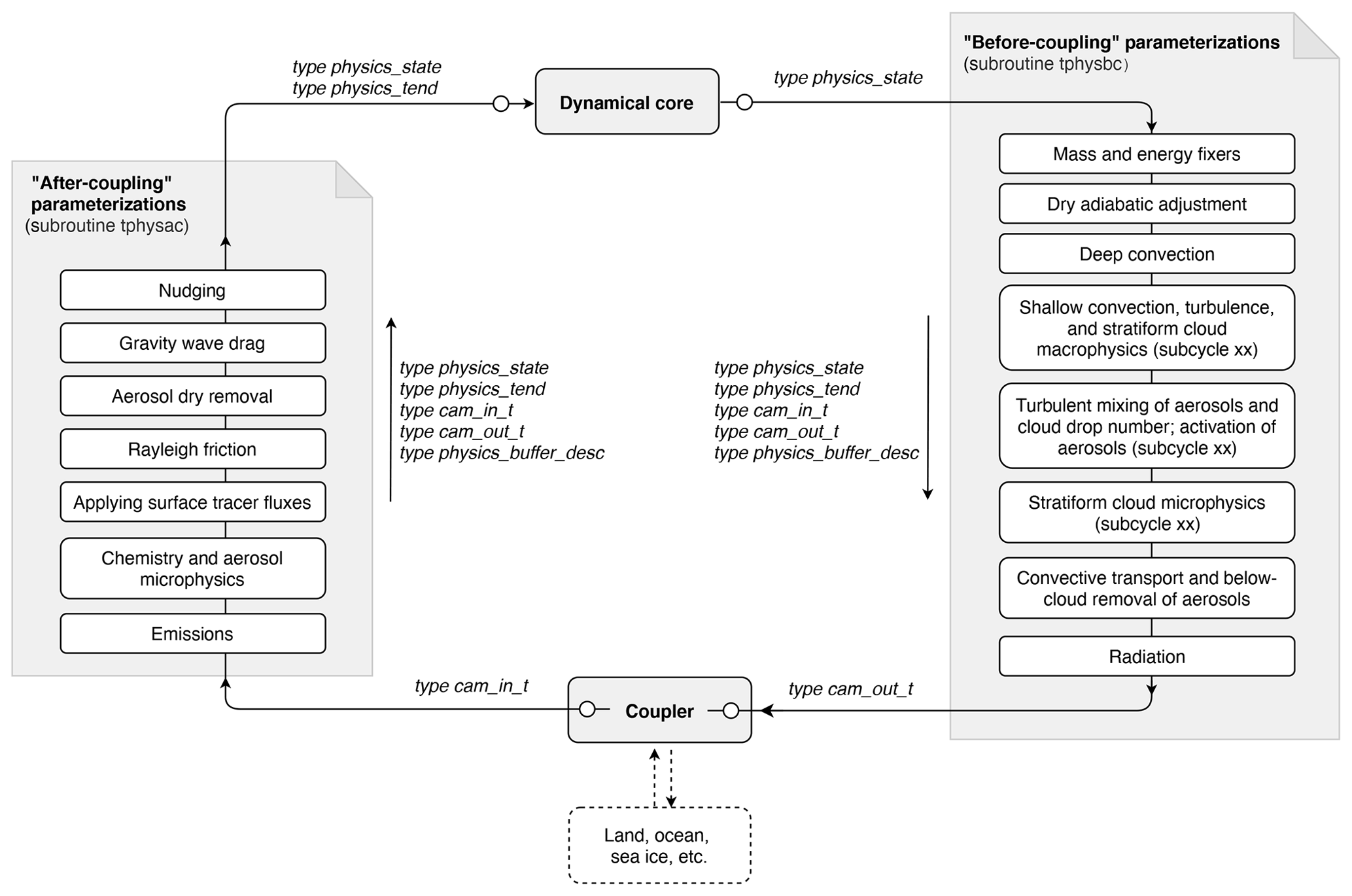
Figure 1A schematic showing the four compartments (gray boxes) of the EAMv1 code: the dynamical core, the coupler, and two groups of parameterizations calculated before or after the communication with the coupler. The derived data types used for passing information among these compartments and within the two groups of parameterizations are shown in italics. The two small circles shown next to the dynamical core and the two circles placed inside the coupler box represent transfer of information to or from data structures internal to the dynamical core or the coupler. The white boxes with solid outlines shown in the “before-coupling” and “after-coupling” parameterization groups are examples (not complete lists) of parameterizations and numerical treatments included in typical EAM simulations.
The new tool was designed for and implemented in EAMv1. It has been ported to EAMv2 and also to a few code versions in between. We expect it to be straightforward to port the tool to EAMv1's recent predecessors, e.g., the Community Atmosphere Model versions 5 and 4 (CAM5 and CAM4, Neale et al., 2012, 2010), as well as their other descendants (e.g., CAM6, Craig et al., 2021), as these models use the same Fortran derived data types for organizing information passed through the physics parameterizations suite. Examples of such Fortran data types include the “physics state”, “physics buffer”, and atmosphere “import” and “export” variables (see Sect. 2.1). It is also possible to revise our tool for implementation in other models, as the underlying design concepts are generalizable (see Sect. 4.4).
The remainder of the paper is organized as follows: Sect. 2 introduces EAMv1's code and data structures as well as the features of the model's time integration and output capability that our tool makes use of. Section 3 introduces the key concepts and basic design of our tool. Section 4 describes the implementation of our tool in EAMv1, and Sect. 5 provides a brief user guide. Section 6 presents three concrete examples to further demonstrate the usage of the tool: a global budget analysis of dust aerosol mass concentration, a composite analysis of sea salt emissions and their dependency on surface wind speed, and a conditionally sampled relative humidity budget. Section 7 summarizes the paper and points out possible future improvements and extensions of the tool.
Here, “host model” refers to the AGCM in which our new tool is embedded, in this case EAMv1. We provide some background information about EAMv1's code structure and data structure in Sect. 2.1 to help explain the implementation and portability of our tool in later sections. We summarize EAMv1's choice of method for coupling atmospheric processes in Sect. 2.2 and briefly describe how model variables are archived on output files in Sect. 2.3. These features of the host mode are used by our tool.
2.1 Data and code structures
EAMv1 is an AGCM consisting of a dynamical core describing the mesh-resolved fluid dynamics
and a suite of parameterizations describing various subgrid-scale processes.
EAMv1 is also the atmosphere component of the coupled Earth system model E3SMv1
(Golaz et al., 2019), and as such,
it communicates with the coupler cpl7 (Craig et al., 2012)
to exchange information with the other components of E3SMv1
such as the ocean model, the land model, and the sea ice model.
Reflecting both perspectives,
the atmosphere model code can be understood as consisting of the four compartments
depicted by gray shaded boxes in Fig. 1:
the dynamical core, the coupler,
and two groups of parameterizations calculated before or after the
communication with the coupler.
The driver subroutines for the before-coupling and after-coupling
parameterization groups are named tphysbc and tphysac,
respectively (Fig. 1).
tphysbc and tphysac
each contain a series of subroutine calls corresponding to
various parameterizations.
The white boxes with solid outlines
in Fig. 1 are examples of such parameterizations.
tphysbc and tphysac
also contain code blocks for
numerical treatments (e.g., total energy fixers or
mass fixers) or for diagnosing quantities of interest.
In the remainder of the paper, we refer to those subroutines
and code blocks as code compartments, too, although
these are sub-compartments of tphysbc and tphysac.
The driver subroutines tphysbc and tphysac
and the code compartments therein are arguably the
code units in EAM that researchers of atmospheric physics most often work with.
EAM's dynamical core and physics driver subroutines use different data structures.
The following derived data types are defined to pass information among the four
compartments shown in Fig. 1 and between parameterizations:
the physics_state type contains variables describing the
atmospheric state
that are passed between the physics and dynamics and between parameterizations.
Examples of such state variables include air temperature, zonal and meridional winds,
vertical velocity, air pressure, pressure layer thickness, geopotential height,
surface pressure, and surface geopotential.
The physics_tend type contains the total tendencies of
temperature and horizontal winds caused by all subgrid processes
as well as a few water and energy fluxes that are passed from the
parameterization suite to the dynamical core.
The import state type cam_in_t and
export state type cam_out_t contain
the fields of physical quantities
that are provided to EAM by the coupler and to
the coupler by EAM, respectively
(see chap. 4 in Eaton, 2015).
The physics_buffer_desc type is defined for constructing
the physics buffer
that contains fields passed between parameterizations.
Dummy variables of these five derived types are
available in subroutines tphysbc and tphysac;
collectively, they describe the characteristics of the model atmosphere
that vary in space and evolve with time.
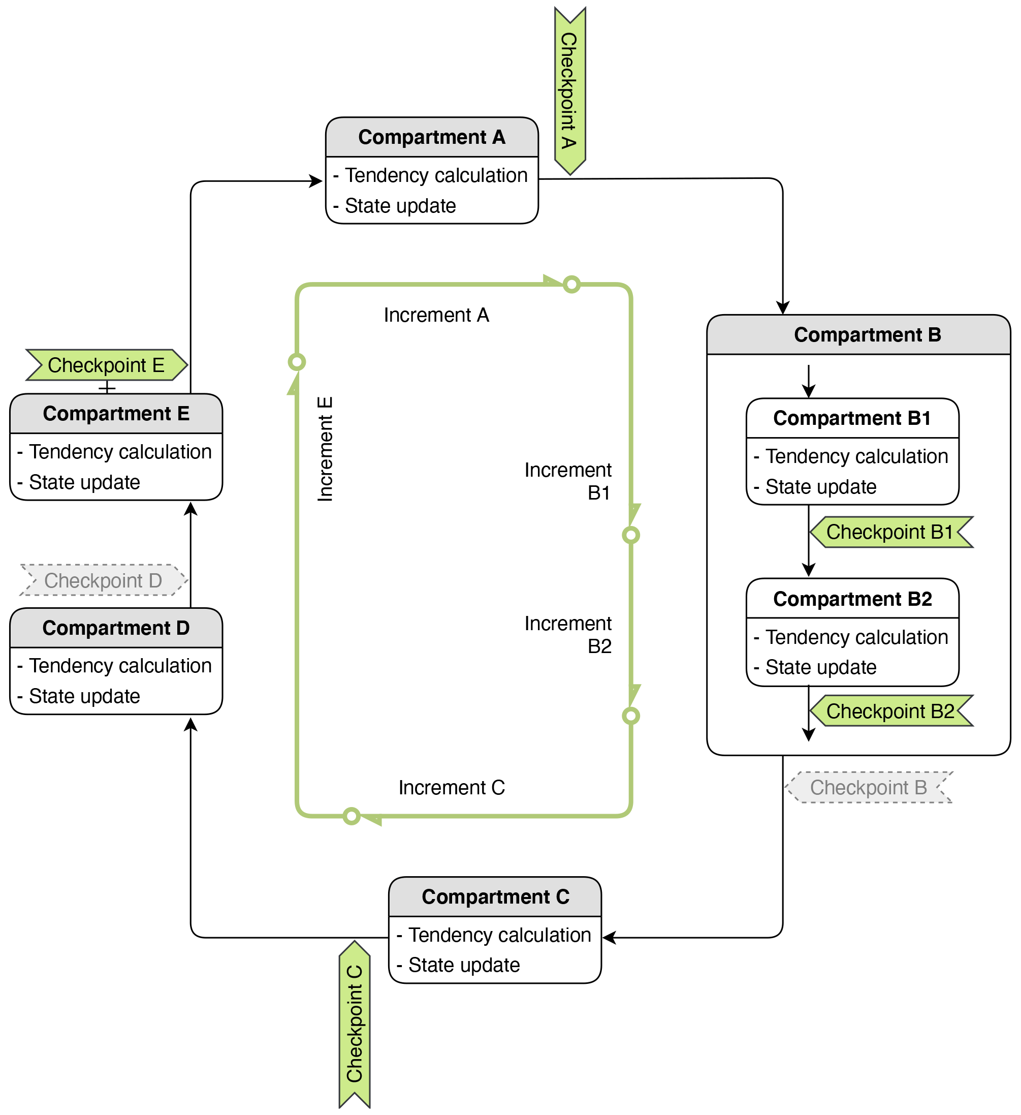
Figure 2A schematic showing a time step of model simulation involving five hypothetical code compartments, A to E, either resolved or unresolved by the model's computational mesh, that are numerically coupled using isolated sequential splitting (see Sect. 2.2). Also shown are various tags of locations (referred to as checkpoints, see Sect. 3.1) within a time step that are introduced to facilitate diagnostics using the new tool. When the tool is used in a simulation, some checkpoints are activated (i.e., selected by the user and indicated in green here), and others are inactive and indicated in gray. No information is monitored at inactive checkpoints. The green lines with a circle on one end and an arrowhead on the other end depict how increments of model variables are defined. Further details can be found in Sects. 2.2 and 3.1.
A subroutine called by tphysbc or tphysac
may again be a driver for a set of closely related parameterizations and
hence calls a number of sub-subroutines. For example,
the chemistry driver in tphysac has multiple levels of subroutines
that correspond to various processes related to chemical gases and
aerosol microphysics. Depending on how those lower-level subroutines
are organized, EAM variables of the derived type physics_state or
physics_buffer_desc may be available in those lower-level
subroutines.
2.2 Sequential process coupling
EAMv1 solves a set of integral–differential equations to simulate the spatial variation and temporal evolution of the state of the atmosphere. Distinct physical and chemical processes (phenomena) are represented by different compartments of the model code. The primary method used in EAMv1 for coupling those compartments is a method we refer to as isolated sequential splitting (Fig. 2). In this method, a code compartment produces an estimate of the rate of change of the atmospheric state by considering a single or a set of closely related physical or chemical processes in isolation (i.e., ignoring all other processes represented by other model components). The estimated tendency is used to update the atmospheric state, and then the updated state is passed to the next code compartment. Since EAMv1 has many code compartments, the atmospheric state is updated multiple times within one full time step. Here a full time step is defined as the smallest time integration cycle in which the effects of all physical processes considered in a simulation have been used to update the model state at least once in advancing the solution in time. This full time step is often loosely referred to as the “physics time step” in EAMv1 and its predecessors. In a discussion on time stepping and subcycling in EAMv1, Wan et al. (2021) referred to the full time steps as the “main process-coupling time steps” and denoted their length by ΔtCPLmain. The same notation is used in this paper for consistency and clarity. The so-called low-resolution configuration of EAMv1 (with 1∘ horizontal grid spacing) uses ΔtCPLmain=30 min by default. Fig. 2 provides a schematic showing a full time step consisting of five hypothetical code compartments labeled A to E.
A code compartment in EAMv1 might contain sub-compartments that are also connected using the isolated sequential splitting method, like compartment B depicted in Fig. 2. A concrete example from EAMv1 is deep convection, which consists of the parameterization by Zhang and McFarlane (1995) that describes the impact of convective activities on temperature and humidity, and a parameterization of the convective momentum transport from Richter and Rasch (2008). These convection-related atmospheric processes are sequentially split within the deep convection parameterization.
Another situation that can also be depicted by the hypothetical compartment B in Fig. 2 is subcycling. For example, in EAMv1, the parameterizations of turbulence, shallow convection, and stratiform cloud macrophysics and microphysics are subcycled six times within each 30 min full time step. In this case, each subcycle can be viewed as a sub-compartment depicted in Fig. 2 (i.e., subcycle 1 corresponds to compartment B1, subcycle 2 corresponds to compartment B2, etc.).
2.3 History output
EAMv1 inherited from its predecessors a flexible mechanism for handling model output (see, e.g., chap. 8 in Craig et al., 2021). The data files that contain the temporal and spatial distribution of model-simulated physical quantities are called history files. The model can write multiple series of history files with different write frequencies; these series are referred to as history tapes in the source code. Different history tapes can contain different output variables (fields). Whether the values written out should be instantaneous, time-averaged, maximum, or minimum during the output time window can be specified for each tape on a field-by-field basis.
The software infrastructure for history output uses internal data types
and functions that handle the storage of fields to be
written out and perform the calculation of required statistics
(e.g., time averages).
Typically,
researchers focusing on physical or computational aspects
of the model do not need to care about the internal workings
of this software infrastructure.
Rather, they use a subroutine named outfld
to transfer the values of a model variable to the infrastructure.
To provide a context for some descriptions in later sections,
we note that while a model variable can change its value multiple times in a time step of ΔtCPLmain, the value being recorded
for output is the snapshot made when the outfld
subroutine is called.
The location in the time integration cycle at which
the outfld subroutine is called can differ
from model variable to variable.
We now introduce the key concepts and design features of the new tool. The description in this section is kept general, only referring to EAM when necessary, as the methodology can be applied to or revised for other AGCMs. Details of the implementation in EAMv1 are provided in Sect. 4.
3.1 Checkpoints, field values, and increments
In order to discuss the implementation of our tool in the context of the sequential process splitting described in Sect. 2.2, we introduce the following nomenclature.
-
A checkpoint is a location in the time integration cycle at which a snapshot of a model variable can be obtained (see Fig. 2). At a checkpoint, the value of a model variable can be retrieved from data structures introduced in Sect. 2.1. Additional quantities can be computed from available variables. Those retrieved or computed variables at the checkpoint can be saved in the data structure specific to our tool and transferred to the output-handling infrastructure of the standard EAM (see Sect. 2.3). If subcycles with respect to ΔtCPLmain are used, then the end of each subcycle is considered to be a different checkpoint.
-
The value of a model variable at a checkpoint is referred to as a field value. For example, the air temperature after compartment A in Fig. 2 is referred to as the field value of temperature at checkpoint A.
-
All checkpoints are inactive by default, meaning no information is retrieved, calculated, or archived by our tool. A checkpoint becomes active when the user selects it at run time (through namelist, see Sect. 5.2.3). This flexibility allows a user to focus only on the checkpoints relevant to their specific study; it also saves memory and disk space, as inactive checkpoints will not consume memory or produce information in the model's output files.
-
The difference between values of the same model variable at two different checkpoints is referred to as an increment. Since there can be inactive checkpoints, an increment calculated by our tool is the difference between the field value at the current checkpoint and the field value at the previous active checkpoint. For example, in Fig. 2, increment E is the difference between checkpoints E and C, with the inactive checkpoint D ignored.
3.2 Composite analysis
For a composite analysis, our tool expects the user to specify one or more conditional sampling criteria via run time input (e.g., namelist parameters). The handling of multiple conditions is described later in Sect. 3.3. Here we first explain the handling of a single sampling condition.
During each time integration cycle of length ΔtCPLmain, values of user-selected variables at active checkpoints are obtained and copied to a data structure internal to our tool. Increments and vertical integrals are calculated if requested. The sampling condition is evaluated at each grid cell in the global domain. Depending on whether the condition is met, the copy of the user-selected variables in our tool's internal data structure, including their increments and integrals if requested by the user, is assigned either the model-computed values or a fill value, resulting in a conditionally sampled copy. This sampled copy, together with information about the sampling condition, is then transferred to the output-handling infrastructure. In the next model time step, the sampling condition is re-evaluated and the user-selected model variables resampled. The details are explained below.
3.2.1 Defining a condition
A key element of a sampling strategy is the atmospheric condition to be used to categorize data. Necessary elements in the definition of a condition include (1) a metric (which can be any 2D or 3D field, e.g., air temperature or surface pressure), (2) a threshold (which is a number, e.g., −40 ∘C or 500 hPa), and (3) a comparison type (e.g., smaller than or equal to). In our tool, a metric can be any prognostic or diagnostic variables in the host model or a quantity that can be diagnosed from existing variables. Currently supported comparison types include (i) <, (ii) ⩽, (iii) >, (iv) ⩾, and (v) equal to within a tolerance. Type (v) can be used to select values within a range. For example, choosing a threshold of −20 ∘C and a tolerance of 20 ∘C would allow the user to sample grid cells with air temperature between −40 and 0 ∘C.
The user's choices of metric, threshold, comparison type, and tolerance (if applicable) are expected to be specified through run time input.
Another key element of the definition of the sampling condition is the location in the time integration cycle at which the sampling condition should be evaluated. As explained earlier in Sect. 2.2, the atmospheric state defined by the prognostic variables of EAM's governing equations is updated multiple times within one full time step of ΔtCPLmain due to the sequential splitting method used for process coupling.
For diagnostic quantities (e.g., relative humidity), the values consistent with the prognostic state also evolve within each time step even though the arrays in the programming language can temporarily contain inconsistent values until the next time of calculation. Because of such evolutions within a time step, our tool requires the user to specify at which checkpoint (see Sect. 3.1) a sampling condition should be evaluated. The implementation of this aspect in EAMv1 is discussed in more detail in Sect. 5.2.1.
Also because of the evolution of model variables within a time step, one needs to be cautious when obtaining values of diagnostic quantities for use by our diagnostic tool. This point is further explained in Sect. 4.1.2.
3.2.2 Condition metric and field of flags
In this first version of our tool, the metric used in defining a sampling condition can be one of the following types of model variables:
-
a 2D field that covers the entire horizontal domain of the model, such as the surface pressure or total cloud cover;
-
a 3D field defined at layer midpoints or as layer averages, e.g., air temperature, cloud fraction, or the mass mixing ratio of a tracer in EAMv1; or
-
a 3D field defined at the interfaces between adjacent layers, e.g., the convective mass flux predicted by the deep convection parameterization or the net longwave radiative flux calculated by the radiation scheme in EAMv1.
For each condition metric, a flag field with the same spatial dimensions is defined in the data structure internal to our tool. After a sampling condition is evaluated at a grid cell in the 2D or 3D domain, the flag field is assigned a value of 1 if the condition is met and a value of 0 otherwise. The flag field, when averaged over time, equals the frequency of occurrence of meeting the sampling condition at each individual grid cell. The flags at different grid cells can be averaged in space, either over the entire 2D or 3D domain or over a subdomain, to calculate the frequency of occurrence of the sampling condition in the corresponding domain, but the spatial averages are expected to be done during post-processing instead of during model integration. A use case example involving both temporal and spatial averaging can be found in Sect. 6.3.
After the sampling condition is evaluated over the entire 2D or 3D domain, the condition metric itself is sampled, meaning that the field of values transferred to the output-handling software contains the model-computed values where the condition is met and a fill value of zero where the condition is not met. In other words, the masking indicated by the flag field is applied to the condition metric as well. Recall that the output-handling infrastructure of EAM supports both instantaneous and time-averaged model output. Since EAM is a climate model, time-averaged output is expected to be used more often. Our tool uses a fill value of zero for archiving the condition metric and the other monitored model variables to make sure that time steps in which the sampling condition is not met make zero contributions to the time average. Later on, during post-processing, when a time average of a condition metric is divided by the time average of the corresponding flag, we get the composite mean, i.e., the average over the time steps when the condition is met.
3.2.3 Monitored model variables
Our tool allows multiple model variables to be monitored under the same sampling condition. To distinguish those monitored variables from the condition metric, the monitored variables are referred to as the quantities of interest (QoIs) in the remainder of this paper and in our code. QoIs monitored under the same condition can have different vertical dimension sizes.
-
When the QoI has the same dimension size as the condition metric, the masking indicated by the flag field can be applied in a straightforward manner.
-
If the metric is 2D and the QoI is 3D, then the same 2D masking is applied to all vertical layers or interfaces.
-
If the metric is 3D and the QoI is 2D, then a grid cell in the 2D domain is selected if any layer midpoint or interface in that column is selected. For example, to quantify the shortwave cloud radiative effect (the QoI) in the presence of ice clouds, one can choose a sampling condition of nonzero ice crystal concentration. Then, if ice crystals occur in any layer in a grid column, the shortwave cloud radiative effect of that grid column will be sampled.
Like the archiving of the condition metric explained in Sect. 3.2.2, a QoI gets a fill value of zero at grid cells wherein the condition is not met so that the composite mean can be derived by dividing the time-averaged QoI by the time-averaged flag field.
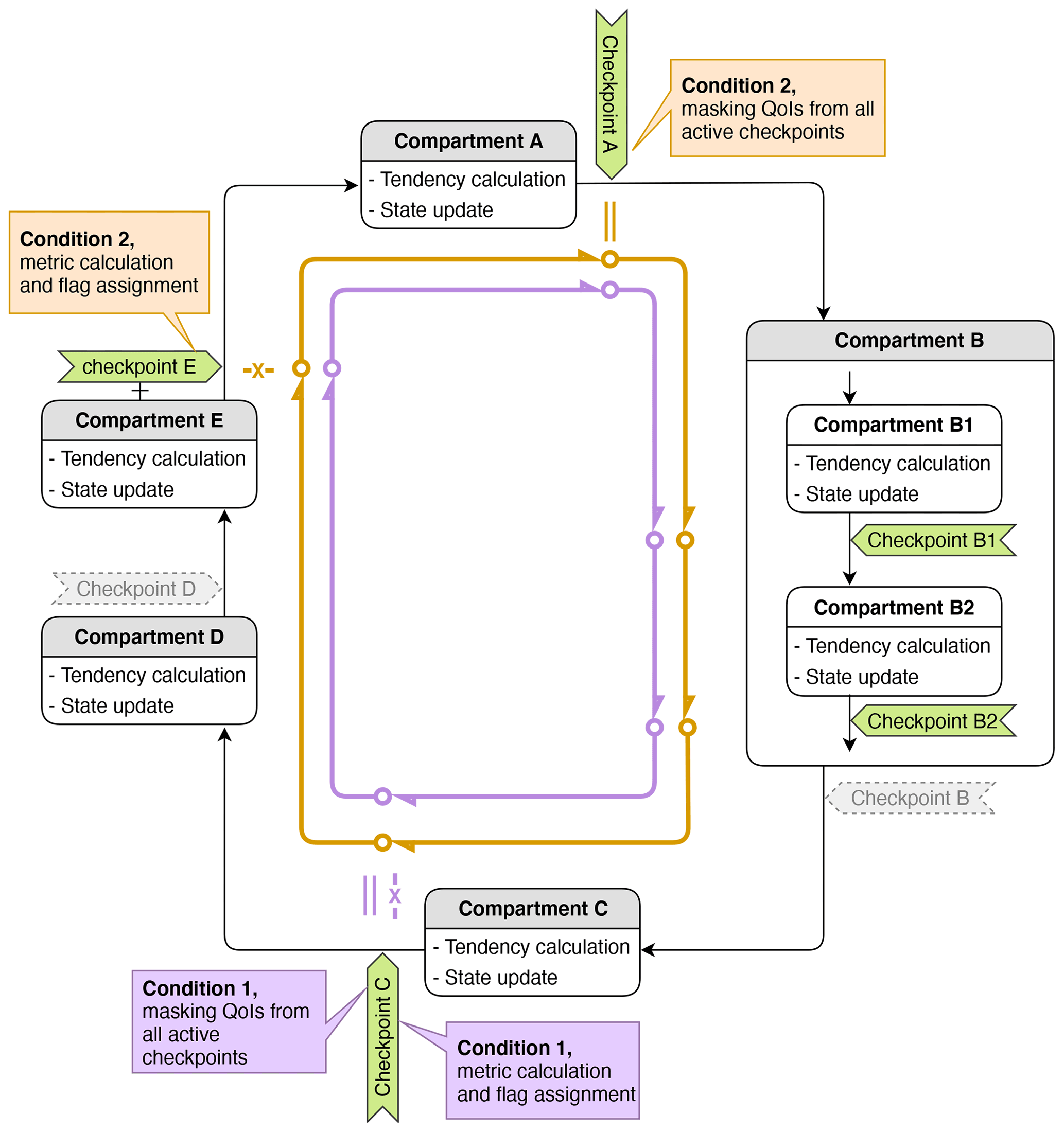
Figure 3A schematic showing two sampling conditions indicated in brown and purple. The “X” marks indicate locations in the time integration cycle at which the condition metrics are evaluated. The double bars indicate the end of validity of the evaluated sampling conditions. More details can be found in Sect. 3.2.4. Like in Fig. 2, green tags are active checkpoints being monitored by the tool. Gray tags with dashed borderlines are inactive checkpoints, which are ignored in the simulation.
3.2.4 Time window of validity of an evaluated condition
Our tool is designed to evaluate a sampling condition once per each ΔtCPLmain at a user-specified checkpoint X, and the tool can monitor QoIs at multiple checkpoints within ΔtCPLmain. By default, the masking resulting from a condition evaluated at checkpoint X is applied retrospectively to all active checkpoints from X until just before the previous encounter of X (i.e., X in the previous time step). This is illustrated by condition 1 shown in purple in Fig. 3, where the sampling condition is evaluated at checkpoint C and the masking is applied retrospectively to checkpoints B2, B1, A, and E.
To provide more flexibility, our tool also allows the user to specify a different checkpoint as the end-of-validity mark for a sampling condition, which we indicate with double bars in Fig. 3. A hypothetical example is given as condition 2 shown in brown in the figure. There, the end-of-validity mark (brown double bar) is placed at checkpoint A, while the sampling condition is evaluated at checkpoint E. The masking determined at E is applied to E and the subsequent checkpoint A, as well as retrospectively to checkpoints C, B2, and B1 before E. An example from EAMv1 showing such usage can be found in Sect. 6.3.
3.3 Multiple sampling conditions in one simulation
A single sampling condition is defined by a combination of (i) a metric, (ii) a threshold, (iii) a comparison type, (iv) a tolerance if the comparison type is “equal to”, (v) a condition-evaluation checkpoint, and (vi) an end-of-condition-validity checkpoint. Changing any of these elements will result in a new sampling condition. Our tool allows multiple conditions to be used in a single simulation (see Fig. 3), and these multiple sampling conditions can use different condition metrics.
For software simplicity, the current implementation only allows one and the same set of QoIs and checkpoints to be monitored under all sampling conditions. In the example illustrated in Fig. 3 where two conditions, conditions 1 and 2, and five active checkpoints (A, B1, B2, C, and E) are activated, let us assume the user has chosen to monitor four QoIs, T, qv, u, and v. The same four QoIs and five checkpoints will be monitored for both sampling conditions. The current implementation does not allow, for example, monitoring only T and qv at checkpoints A and C under condition 1 and only u and v at checkpoints A, B1, and B2 under condition 2, although this kind of flexibility can be considered for future versions of CondiDiag if needed.
Since the current implementation monitors the same QoIs for all sampling conditions in the same simulation, one can run into a situation in which the metric and the QoI are both 3D fields but have different numbers of vertical layers (e.g., the metric is the air temperature defined at layer midpoints, while the QoI is the net longwave radiative flux defined at layer interfaces). In such a case, masking will be skipped, meaning this specific QoI will be captured for output as if no conditional sampling had happened.
3.4 Mass-weighted vertical integral of QoIs
For spatially 3D QoIs defined at layer midpoints or as cell averages, the vertical integral weighted by air mass can be calculated during the time integration and then conditionally sampled and written out as 2D variables. This applies to both field values and their increments.
One caveat is that in EAM's physics parameterizations, the mixing ratios of water species (vapor, cloud liquid and ice, rain, and snow) are defined relative to the mass of moist air (i.e., dry air plus water vapor), while the mixing ratios of aerosols and chemical gases are defined with respect to dry air. Our tool expects the user to specify which kind of air mass (moist or dry) should be used for each QoI when vertical integrals are requested (see Sect. 5.2.4).
This section explains how the design features described in Sect. 3 are implemented in EAMv1. We provide an overview of the new Fortran modules added specifically for the tool (Sect. 4.1), introduce a general-purpose diagnostics module (Sect. 4.2) and summarize the changes made to the original EAMv1 code (Sect. 4.3). We keep these sections brief but provide two versions of the EAMv1 code on Zenodo (https://doi.org/10.5281/zenodo.6325126, Wan et al., 2022) corresponding to the GitHub commits before and after the implementation of CondiDiag1.0 so that readers can review the details of the code changes if needed.
The Zenodo archive also contains a third tar ball containing only the source files that were added or revised during the implementation of CondiDiag1.0, as well as a copy of the original version of the revised EAMv1 files.
4.1 CondiDiag-specific new modules
Four new modules are added to define data structures and support key functionalities of our diagnostic tool. These are briefly described below.
4.1.1 Data structure module
The module conditional_diag contains definitions of the basic data structures
used by our tool and subroutines for initializing the corresponding Fortran variables.
A Fortran variable cnd_diag_info of the derived type
cnd_diag_info_t contains the metadata that describe the
user's conditional sampling strategy and budget analysis configuration.
A namelist conditional_diag_nl (see Sect. 5.2)
is also defined in this module, and
a subroutine cnd_diag_readnl parses the user's namelist
input and populates the information to
cnd_diag_info.
A second derived type cnd_diag_t is defined for storing
the values of the metrics, flags, and the field values and increments of QoIs.
The corresponding Fortran variable is an array named phys_diag;
the array is defined in a different module (explained in Sect. 4.3.1).
The subroutines that allocate memory for elements of phys_diag
and their components are included in module conditional_diag.
4.1.2 Key algorithm module
The module conditional_diag_main contains the key subroutine
of our tool, named cnd_diag_checkpoint, which obtains the values of
the condition metrics and QoIs, calculates the QoI increments,
evaluates the sampling conditions, applies conditional sampling,
and transfers the sampled fields to the output-handling infrastructure of EAM.
Examples showing how the subroutine is invoked in EAM are explained
in Sect. 4.3.2.
As mentioned earlier in Sect. 3.1, the condition metrics and QoIs
can be existing components of EAM's state variable, physics buffer, and
the atmosphere import and export data structures
(see Sect. 2.1; note that
the physics_tend type is not used by our tool).
For example, air temperature is a component of the atmosphere state variable;
hence, the values are retrieved in
subroutine get_values in module
conditional_diag_main by the following code block.
 case('T')
   arrayout(1:ncol,:) = state%t(1:ncol,:)
Condition metrics and QoIs can also be physical quantities that need to be calculated from components of EAM's existing data structures. For example, the relative humidity with respect to ice is obtained by the following code block.
 case ('RHI')
   call relhum_ice_percent(  &
        ncol, pver,          &! intent(in)
        state%t(:ncol,:),    &! intent(in)
        state%pmid(:ncol,:), &! intent(in)
        state%q(:ncol,:,1),  &! intent(in)
        arrayout(:ncol,:)    )! intent(out)
In these examples, “T” and “RHI” need to be unique names
within the module conditional_diag_main;
these will also be the metric or QoI names that the users refer to
in the namelist conditional_diag_nl (see Sect. 5.2).
The currently implemented metric and QoI names
are listed in Table A1 in
Appendix A.
Additional metrics and QoIs can be added
following the existing examples.
We note that some of the variable names in
Table A1 coincide with
EAM's standard history variable names, but the coincidence
has no significance.
Because a QoI can be monitored at different checkpoints
and under different conditions, those different combinations
will each correspond to a distinct variable name in the history files,
as explained in Sect. 4.1.3.
Here, it is worth pointing out one important caveat for obtaining values of
diagnostic quantities in the host model.
As mentioned in Sect. 3.2.1,
the values of diagnostic quantities
that are consistent with the prognostic state effectively evolve within a full model time step,
but the arrays in the programming language might
have only one or a few updates per full time step
and can hence temporarily have inconsistent values.
Care is needed to handle
the corresponding code blocks in subroutine get_values of module
conditional_diag_main.
Let us assume the host model has a diagnostic quantity whose value
is saved in the physics buffer under the name ABC.
If the user's intention is to understand the host model's code
by tracking when the physics buffer's component ABC
is updated within a full model time step,
a code block like the following is needed.
 case('ABC'//'_PBUF')
   idx = pbuf_get_index('ABC')
   call pbuf_get_field( pbuf, idx, ptr2d)
   arrayout(:,:) = ptr2d
If the user's intention is to understand the physics
by monitoring the values of ABC that are consistent with the evolving
prognostic state, a code block like the following is needed,
which recalculates the value of ABC from the state variable.
 case('ABC'//'_EVOL')
   call calculate_abc( state, ..., arrayout)
The RHI budget example shown in Sect. 6.3 falls into the second category.
4.1.3 History output module
The module conditional_diag_output_utils is responsible for
adding the following items to EAM's master list of history output variables:
-
the conditionally sampled metric field named with the pattern
cnd<index>_<metric_name> where <index> is a two-digit number (e.g.,cnd01_Tif the first sampling condition uses air temperature as the metric); -
the flag field (see Sect. 3.2.2) named
cnd<index>_<metric_name>_flag; -
one output variable corresponding to each QoI at each active checkpoint under each sampling condition, named with the pattern
cnd<index>_<QOI_name>_<checkpoint_name> (for example,cnd01_CLDLIQ_DYNENDis the stratiform cloud liquid mixing ratio monitored at checkpoint DYNEND under condition 1; if increments of the QoI are calculated and archived, these will be named similarly to the QoIs but with a suffix_incappend, e.g.,cnd01_CLDLIQ_DYNEND_incfor the increment of CLDLIQ at checkpoint DYNEND under condition 1). -
If the mass-weighted vertical integral is requested for a QoI, then a suffix
_vwill be appended to the QoI name. For example,cnd01_CLDLIQ_v_DYNENDis the column burden of CLDLIQ at checkpoint DYNEND under condition 1, andcnd01_CLDLIQ_v_DYNEND_incis the corresponding increment.
We expect that users of our tool should not need to touch
the conditional_diag_output_utils module
unless they want to
revise the naming conventions for variables in the history files.
It is worth noting that for any of the output variables added by our tool, EAM's standard history output functionalities apply (see Sect. 2.3). For example, each variable can be added to or excluded from one or multiple history tapes and be written out at the user-specified frequencies. For temporal statistics, both instantaneous and time averages can be used in the current implementation. Maximum and minimum values need to be used with care as unselected grid cells are filled with zeros. In future versions, we will consider allowing the user to specify what missing value should be assigned to each QoI.
4.1.4 Restart module
Because our diagnostic tool uses its own data structure,
new subroutines have been included to add additional contents to
EAM's restart files. These subroutines
are placed in the module conditional_diag_restart.
As long as a user does not change the data structures
defined in module conditional_diag, there should
be no need to touch the restart module even if they
add new metrics and QoIs to the key algorithm modules
conditional_diag_main and misc_diagostics.
4.2 General-purpose diagnostics module
We imagine a user might want to provide their own subroutines
to calculate new metrics or QoIs that are not available in the host model
or recalculate diagnostic quantities
to obtain values consistent with the evolving prognostic state
(like relhum_ice_percent
in the code snippet in Sect. 4.1.2).
In such cases, we recommend those subroutines be placed in the module
misc_diagnostics rather than in
conditional_diag_main
because we view those user-provided subroutines
as general-purpose diagnostic utilities that
could also be used by other parts of EAM (e.g.,
in some parameterizations for diagnostic purposes).
4.3 Other code changes in EAMv1
Apart from adding the five modules explained in Sects. 4.1 and 4.2, the implementation of our tool in EAMv1 only involved a very small number of code changes, as described below.
4.3.1 The phys_diag array and its elements
Our tool uses its own derived data type
cnd_diag_t for storing
values of the condition metrics, flags, and the
field values, increments, and vertical integrals of QoIs
(see Sect. 4.1.1).
The data storage closely follows
the handling of EAM's model state variable.
To explain the background, we note that
in order to parallelize the parameterization calculations on supercomputers,
EAM's global domain is divided into “chunks” of grid columns.
A chunk contains a compile-time configurable number of columns that
are not necessarily neighbors in the geographical sense.
Each call of tphysbc or tphysac performs calculations
of the corresponding parameterizations in a single grid chunk,
while each MPI (Message Passing Interface) process on the supercomputer
typically performs calculations
for multiple chunks (see chap. 4 in Eaton, 2015).
In tphysbc and tphysac,
the dummy variable state
is declared as a scalar of type physics_state,
and this scalar contains data for a single grid chunk.
The parent routines of tphysbc and tphysac
declare rank-one arrays (of type physics_state)
named phys_state for storing data
for all chunks handled by the same MPI process.
Similarly, for implementing our tool in EAMv1,
rank-one arrays of type cnd_diag_t named phys_diag
are declared in parent routines of tphysbc and tphysac.
The scalar variable of type cnd_diag_t in
tphysbc or tphysac is named diag.
4.3.2 Checkpoints
The checkpoints listed in Tables B1 and B2
in the Appendices have been added to tphysbc and tphysac
by inserting code lines like the following code block.
  call cnd_diag_checkpoint( diag, &! inout
       'DYNEND', state, pbuf,     &! in
       cam_in, cam_out            )! in
These code lines are inserted after the white boxes with solid outlines shown in Fig. 1.
Here, diag is the scalar variable of type cnd_diag_t
explained in Sect. 4.3.1;
DYNEND is the unique string identifying this checkpoint, and
state, cam_in, and cam_out are scalar
variables of derived types declared in the original EAM code.
As mentioned in Sect. 2.1,
the EAM code has a hierarchical structure;
the state, cam_in and cam_out
variables as well as the physics buff are also available
in some lower-level routines called by the physics drivers
tphysbc and tphysac. Checkpoints can be
added to those lower-level routines.
To demonstrate this point, in CondiDiag1.0,
checkpoints have been included in the stratiform cloud
macrophysics driver subroutine clubb_tend_cam in the form of, e.g., the following code block.
 call cnd_diag_checkpoint( diag,    &! inout
      'CLUBB'//char_macmic_it,      &! in
      state1, pbuf, cam_in, cam_out )! in
The character string char_macmic_it labels
the subcycle within a full time step ΔtCPLmain.
It is worth emphasizing that
state1 (instead of state)
is referred to in the code snippet quoted above
because state1 is the atmospheric state variable
that is sequentially updated by various code blocks (compartments) in
clubb_tend_cam.
4.4 Portability
Our new tool was originally developed for and implemented in version 1 of EAM and was then tested in v2 and some in-between versions. The porting turned out to be straightforward as the basic code and data structures in EAM had not changed. To implement CondiDiag in models outside the EAM/CAM model families will require some significant adaptation. Some thoughts are shared here.
We assume the host model has a few high-level driver subroutines (or one driver) that organize code compartments corresponding to various atmospheric processes. This, to our knowledge, is common in AGCMs.
Our code also makes use of the fact that the drivers use derived data types to organize a large number of model variables of interest for physics-oriented or numerics-focused studies. These derived data types make our code more flexible and compact, especially for conditional sampling.
For performing budget analysis, our current algorithm assumes the sequential splitting method is used in the host model. For models that use different coupling methods (e.g., parallel splitting or a mixture of methods), it might be possible to obtain the budget terms directly from the tendencies saved in existing model variables.
The four new modules CondiDiag introduces to EAM (see Sect. 4.1) all use some EAM-specific data structures and software functionalities. For porting to a new model, some parts of these modules will be straightforward to port and the other parts will need a rewrite.
The conditional_diag module has the weakest dependency on EAM.
The metadata-handling part
(i.e., parsing the user's choices of QoIs, metrics, etc.)
is independent of EAM's data structures. The module also
contains a few subroutines that allocate memory for the derived-type
arrays used for storing the QoIs and metrics.
The code therein assumes a chunk-based domain decomposition, which likely
will need to be adapted to the new host's data structure.
The conditional_diag_main module contains
subroutines for retrieving field values, deriving increments,
calculating vertical integrals, and performing conditional sampling.
The subroutines assume all QoIs and condition metrics can be
retrieved or recalculated from EAM-specific data structures
described in Sect. 2.1;
hence, the dummy variables and their usage will need to be
adapted for a new host model.
Module conditional_diag_output_utils
and module conditional_diag_restart
will each need a rewrite for a new host.
The key task of the subroutines therein is to
do I/O for all components of the derived type cnd_diag_t.
We expect that one needs to follow the host model's way
of handling I/O for 2D and 3D variables.
The rewrite will likely be somewhat tedious but presumably
not difficult.
The new tool is expected to be useful for a wide range of simulations routinely performed by the model developers and users, including debugging simulations that are a few time steps long, short few-day simulations for preliminary testing, or weather-forecast-style simulations for comprehensive evaluations of the model physics following protocols like Transpose-AMIP (e.g., Phillips et al., 2004; Williams et al., 2013; Williamson et al., 2005; Martin et al., 2010; Xie et al., 2012; Ma et al., 2013, 2014), as well as more traditional multi-year to multi-decade simulations.
To obtain process-level understanding of model behavior, it can be useful to use the new tool in an iterative manner. For example, for a study like Zhang et al. (2018) wherein one needs to identify code compartments that result in negative values of specific humidity, we can start by carrying out a few-day or 1-month simulation with unconditional sampling and choosing a large number of checkpoints to monitor code compartments that are expected to affect humidity or might inadvertently do so because of computational artifacts or code bugs. We let the tool diagnose and archive time averages of the specific humidity and its increment at these checkpoints to get a sense of typical values of the state variable and identify sources and sinks of moisture. In a second step of investigation, we eliminate from the previous selection any checkpoints that have been confirmed to not show humidity change in any grid cell or time step in the few-day or 1-month simulation. From the shorter list, we can pick one or multiple code compartments as suspected culprits of negative specific humidity. If m suspects are selected for further investigation, then m sampling conditions can be specified in the next simulation, all using qv<0 as the sampling criterion but each evaluated after a different suspect. We can also select some QoIs (e.g., temperature, specific and relative humidity, wind, total cloud fraction, cloud liquid and ice mixing ratios) to monitor both right before and right after the code compartments that are suspected to cause negative water vapor. We can request both the field values and increments of these QoIs to be archived as time averages, instantaneous values, or both. This second step might provide useful clues about the typical meteorological conditions under which negative water vapor is predicted in the model. If pathological conditions are identified, then we can carry out additional simulations using relevant sampling conditions to further investigate the causes of those pathologies.
This section explains how investigations described above can be performed using our tool. We first present a typical workflow in Sect. 5.1 to illustrate the steps that a user needs to go through when designing an analysis and setting up an EAM simulation using our tool. We then explain the namelist parameters of our tool in Sect. 5.2.
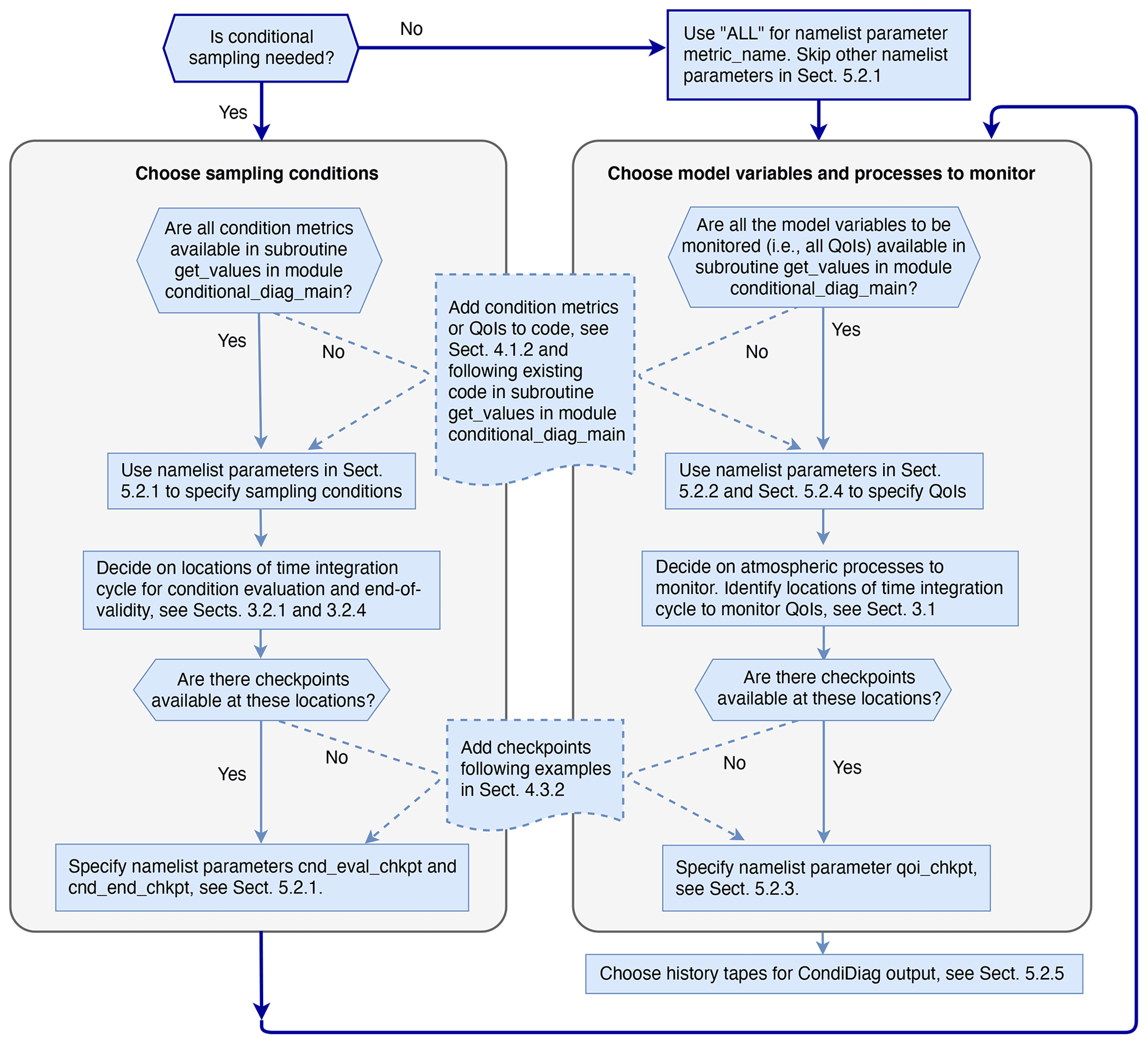
Figure 4A schematic showing the typical steps a user needs to go through for setting up an EAM simulation with online conditional sampling or budget analysis enabled using our tool. Dashed lines indicate places where code changes or additions are needed from the user.
5.1 User workflow
The schematic in Fig. 4 summarizes the steps to take for designing a composite or budget analysis using our tool. It also points to relevant concepts explained in earlier sections and namelist parameters explained below.
5.2 Namelist conditional_diag_nl
Users specify their
conditional sampling and budget analysis strategy
via the namelist
conditional_diag_nl, which
consists of five groups of parameters.
5.2.1 Specifying sampling conditions
For the specification of sampling conditions, we have
-
metric_name, a character array containing the names of the condition metrics to be used in a simulation; -
metric_nver, an integer array specifying the number of vertical levels of each metric (this is meant to help distinguish physical quantities that (1) have no vertical dimension, (2) are defined at layer midpoints, and (3) are defined at layer interfaces; valid values for metric_nver are 1,pver(e.g., 72), andpverp(e.g., 73), wherepverandpverpare EAM's variable names for the number of vertical layers and interfaces, respectively); -
metric_cmpr_type, an integer array specifying the types of comparison to be used for each condition (one entry per condition: 0 for “equal to within a tolerance”, 1 for “greater than”, 2 for “greater than or equal to”, −1 for “less than”, and −2 for “less than or equal to”); -
metric_threshold, a double-precision floating-point array specifying the threshold values that the metrics will be compared to (one threshold for each condition); -
metric_tolerance, a double-precision floating-point array specifying the tolerances for conditions with comparison type 0 (one tolerance for each condition; the value will have no effect for conditions with a nonzero comparison type); -
cnd_eval_chkpt, a character array specifying at which checkpoints the conditions will be evaluated (see Sect. 3.2.1; one checkpoint for each condition); -
cnd_end_chkpt, a character array specifying the checkpoints defining the end of validity of an evaluated condition (see Sect. 3.2.4; one checkpoint per condition). If not specified by user, the end-of-time-step checkpoint will be set to the condition-evaluation checkpoint (cnd_eval_chkpt).
5.2.2 Specifying monitored model variables
The QoIs to be monitored are specified via a character
array qoi_name. The number of vertical levels of
each QoI is specified through the integer array qoi_nver.
If no QoIs are specified but some sampling conditions have been
chosen, then conditional sampling will only be applied to the metrics.
The monitoring of QoI field values is turned on by
the logical scalar l_output_state.
A second logical scalar, l_output_incrm,
is used to turn on or off the monitoring of QoI increments.
User choices for the two switches will be applied to all QoIs.
5.2.3 Choosing checkpoints
The checkpoints at which the QoIs will be monitored are specified by
a character array qoi_chkpt.
The sequence in which they are mentioned in the namelist has no significance.
Note that the same checkpoints are applied to all QoIs.
Also note that if the user specifies a checkpoint name that does not
match any checkpoint implemented in the code (e.g., because of a typographical error),
then our tool will act as if the wrong checkpoint is an inactive one
– in the sense that it will get ignored when the tool
attempts to obtain QoI field values and calculate increments
as the simulation proceeds;
the history files will contain output variables corresponding to
the incorrect checkpoint name, but those output variables
will contain zeros.
5.2.4 Turning on vertical integral
The calculation of mass-weighted vertical integrals of QoIs can be enabled
by the integer array qoi_x_dp.
The values are specified in relation to
qoi_name, i.e., one value of qoi_x_dp for each QoI.
A value of 0 is interpreted as no integral; the QoI will be sampled and written out
as a 3D field. If 1 (moist) or 2 (dry) is selected,
the corresponding (moist or dry) air mass will be used for the vertical integral of
that QoI at all active checkpoints in the simulation.
If the user wishes to monitor both a 3D QoI and its vertical integral,
they can specify the same QoI twice in qoi_name
and set one of the corresponding elements in the qoi_x_dp array to 0
and the other to an appropriate value (1 for moist and 2 for dry)
to request a vertical integral.
A use case example is provided in Sect. 6.1.
For budget analyses in which mass conservation error
is an important topic, there are some nuances related to the
fact that the aerosol and chemical gas mixing ratios
are converted from drying mixing ratios to moist mixing
ratios close to the end of tphysac.
This is further discussed in Appendix C.
5.2.5 Turning on history output
A user might want to write out multiple
copies of the conditional diagnostics or budget diagnostics
to different history files
corresponding to different output frequencies or temporal averaging.
To support such needs, the integer array
hist_tape_with_all_output specifies
which history files will contain
the full set of output variables from our tool.
For example, hist_tape_with_all_output = 1, 3
will include the output to the h0 and h2 files.
Again, we note that the standard output
functionalities in EAM explained in Sect. 2.3 still apply.
5.3 Using unconditional sampling
One of the main motivations for creating our tool is to facilitate budget analysis. If an analysis is to be carried out for the entire computational domain and all time steps, then a special metric named ALL can be used. In such a case, the user can ignore (skip) the other namelist parameters in Sect. 5.2.1. When ALL is used, the condition evaluation will be skipped during the model's integration (see example in Sect. 6.1). Another way to use unconditional sampling is to specify a condition that will always be fulfilled (e.g., relative humidity higher than −1 %). A use case example is provided in Sect. 6.3.
This section demonstrates the usage of the new tool using three concrete examples.
The first example is a global budget analysis without conditional sampling. It demonstrates how to request unconditional sampling and how to request that increments of model variables be calculated and archived as time averages. This first example also demonstrates that with our tool, it is convenient to obtain both vertical profiles and vertical integrals of the budget terms.
The second example is a composite analysis without budget terms. It demonstrates how to use multiple sampling conditions in the same simulation and also shows that the tool can be used to perform a univariate probability distribution analysis.
In the third example, the increment diagnosis and conditional sampling capabilities are combined to perform a conditional budget analysis. The example demonstrates how metrics and monitored QoIs can be chosen to be physical quantities that need to be calculated from the host model's state variables using user-provided subroutines.
The examples shown here use 1-month simulations of October 2009 with monthly (or monthly and daily) output. All simulations were carried out with active atmosphere and land surface as well as prescribed sea surface temperature and sea ice concentration at 1∘ horizontal resolution with out-of-the-box parameters and time integration configurations of EAMv1.
6.1 A global budget analysis of dust aerosol mass mixing ratio and burden
The first example is a global dust aerosol mass budget analysis without conditional sampling. The simulation is designed to provide insight into the atmospheric processes that change the burden (vertical integrals) of dust aerosols in two size ranges (accumulation mode and coarse mode). In particular, we are interested in dust emission, dry removal (i.e., sedimentation and dry deposition at the Earth's surface), resolved-scale transport, subgrid-scale turbulent transport and activation (i.e., nucleation scavenging), the wet removal caused by precipitation collecting particles by impaction, and resuspension caused by evaporation of precipitation.
Table 1Namelist setup used in the dust budget analysis example in Sect. 6.1.
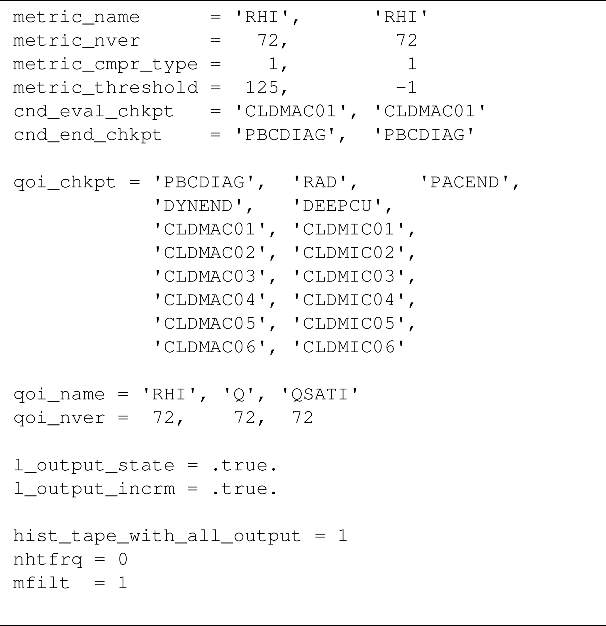
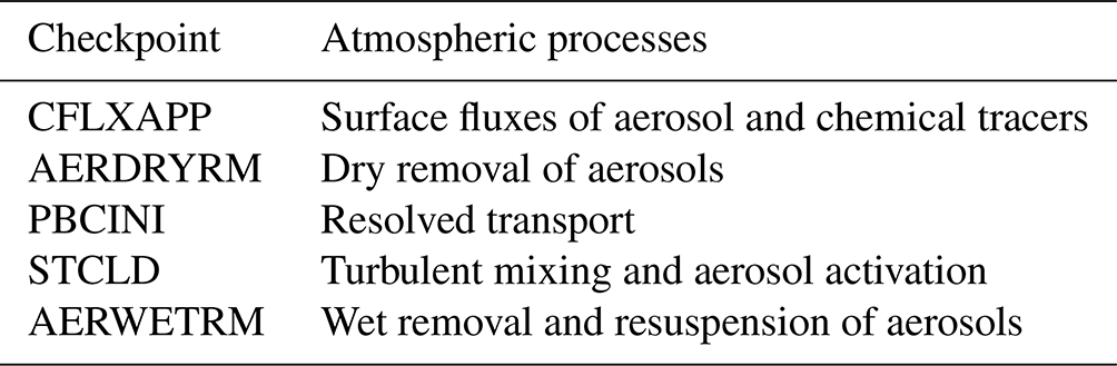
Table 2For the dust budget analysis example in Sect. 6.1: atmospheric processes corresponding to increments diagnosed at the checkpoints selected in the namelist shown in Table 1.
6.1.1 Simulation setup
The namelist setup for this study is shown in Table 1. Only one condition is specified: the special metric ALL is used to select the entire model domain and all time steps.
The QoI names dst_a1 and dst_a3 are EAM's tracer names
for dust mass mixing ratio in the accumulation mode and coarse mode, respectively.
Each tracer name is mentioned twice under qoi_name,
with corresponding qoi_x_dp values of
0 and 2, meaning that both the vertical distribution
of the tracer and its column burden are monitored.
With l_output_state set to .false.
and l_output_incrm set to .true.,
the tool captures the dust mass mixing ratio increments
caused by the targeted atmospheric processes but not the mixing ratios.
Five checkpoints are chosen for monitoring the dust budget.
The corresponding atmospheric processes are listed in
Table 2.
(We remind the users that,
as shown in Fig. 2,
the code compartments that contribute to increments
diagnosed at a checkpoint not only depend
on where this checkpoint is located in the time integration cycle
but also where the previous active checkpoint is located.)
The full set of fields tracked by our tool is sent to output files 1 (the h0 file) and 2 (the h1 file), with the h0 file containing monthly averages and the h1 file containing daily averages.
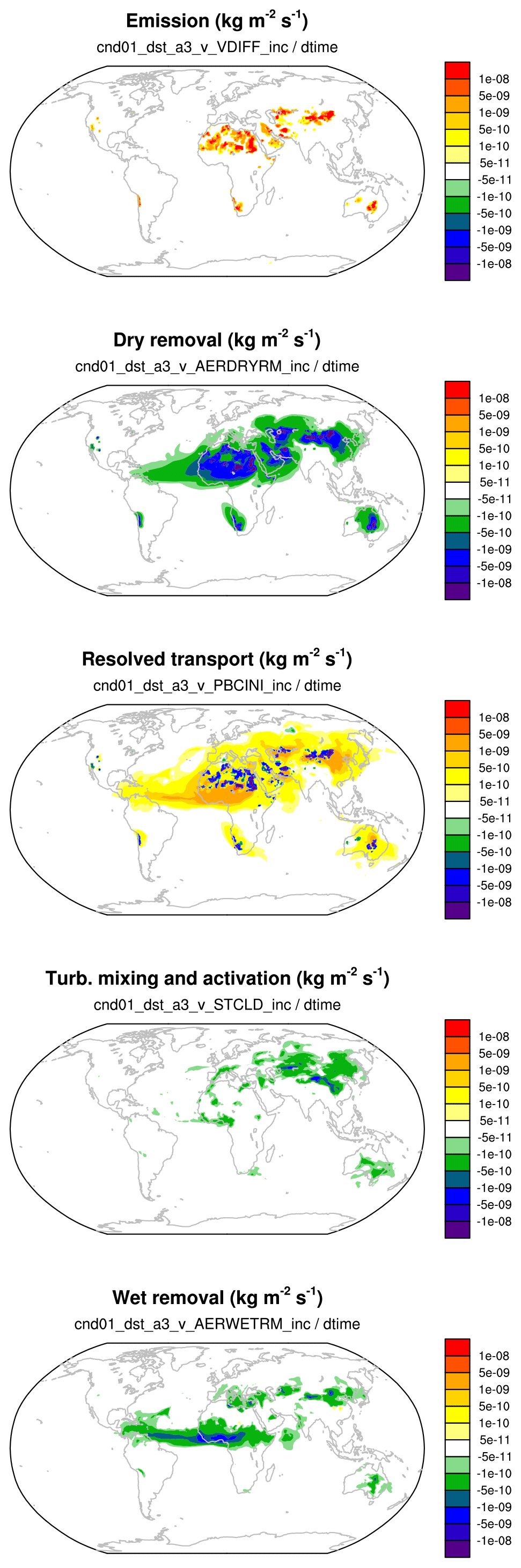
Figure 5The 1-month mean tendencies of the vertically integrated coarse-mode dust burden (unit: kg m−2 s−1) attributed to different physical processes in EAMv1. The expressions given below panel titles indicate how the presented quantities are calculated from the model's output variables.
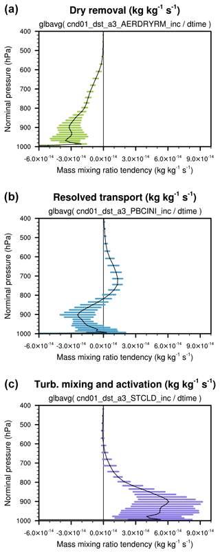
Figure 6Globally averaged vertical profile of the coarse-mode dust mass mixing ratio tendencies (unit: kg kg−1 s−1) attributed to dry removal (a), resolved transport (b), and the turbulent mixing and activation of aerosol particles (c). The black curves are monthly averages. The lengths of the horizontal bars correspond to twice the standard deviation of the daily averages. The expressions given below panel titles indicate how the global averages are calculated from the model's output variables.
6.1.2 Results
Figure 5
shows a 1-month mean geographical distribution of the
sources and sinks of dust mass in the coarse mode (unit: kg m−2 s−1).
The values shown are the output variables
cnd01_dst_a3_v_<checkpoint_name>_inc in the h0 file
divided by ΔtCPLmain=30 min.
Figure 6
shows examples of the globally averaged vertical profiles of
the coarse-mode dust mass mixing ratio tendencies
(unit: kg kg−1 s−1).
The black curves are monthly averages.
The colored horizontal bars indicate
variability of the daily averages derived
from the 3D increment fields
cnd01_dst_a3_<checkpoint_name>_inc written to the h1 file.
6.2 A composite analysis of sea salt emissions in relation to surface wind speed
This example demonstrates the use of composite analysis (without budget terms) to provide insight into wind speed impacts on emission fluxes of sea salt aerosol in various size ranges. The intention is to examine the geographical distribution of sea salt emission fluxes under weak, medium, and strong wind conditions and quantify their relative contributions to the total emission fluxes.
Table 3 Namelist setup used in the composite analysis presented in Sect. 6.2.
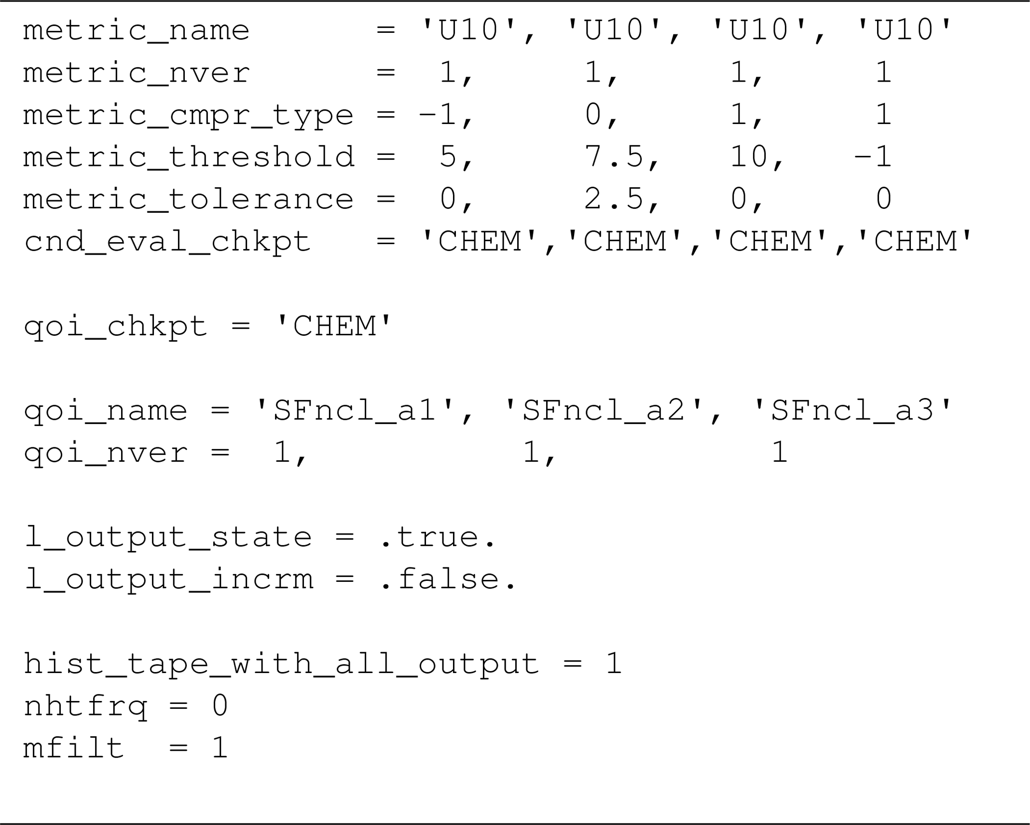
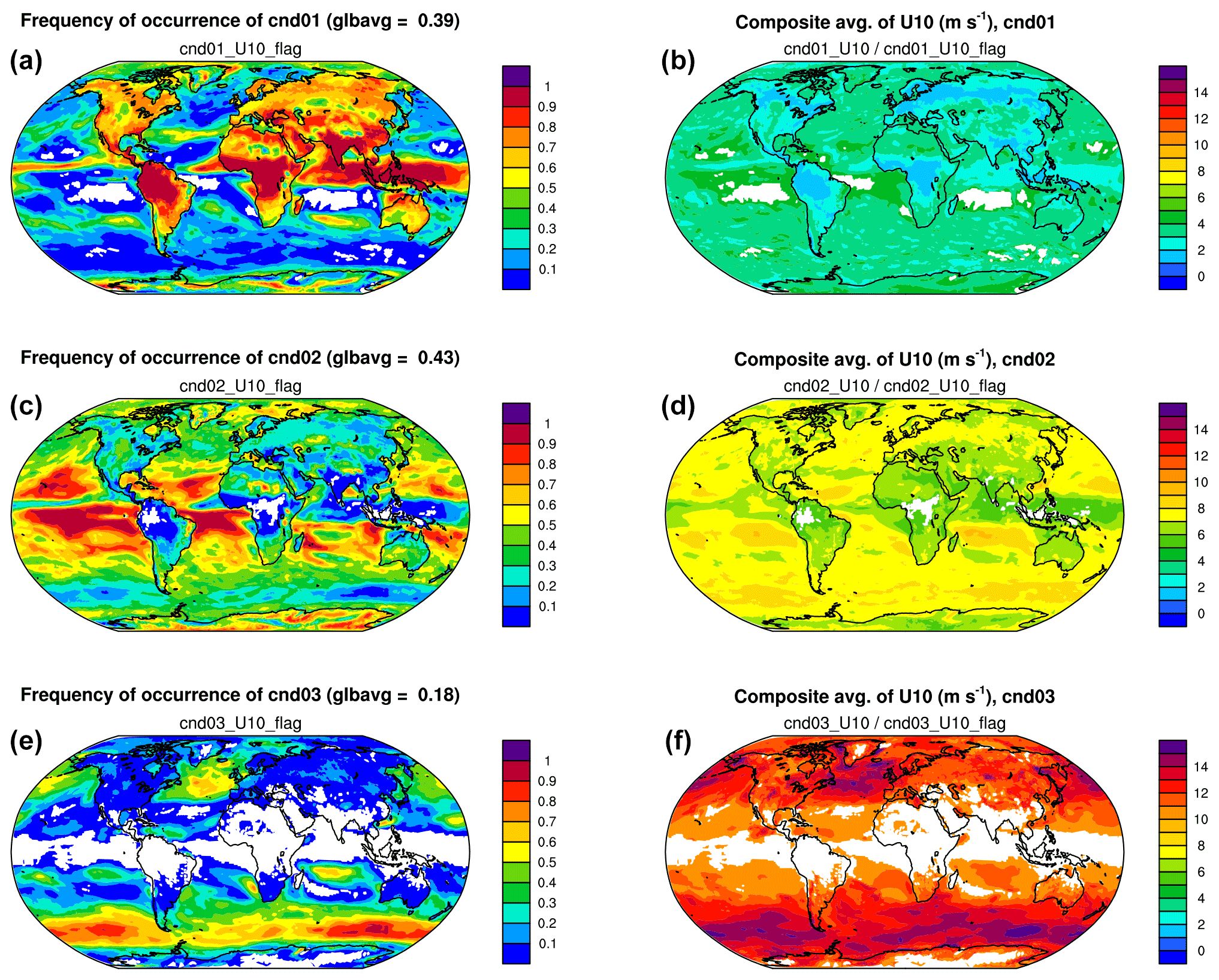
Figure 7(a, c, e) Geographical distributions of the frequency of occurrence of conditions 1–3 corresponding to 10 m wind speed (U10) <5 m s−1 (a, b), between 5 and 10 m s−1 (c, d), and >10 m s−1 (e, f). (b, d, f) Composite average of U10 under each condition. White areas in the contour plots correspond to no occurrence of condition in the 1-month simulation. The expressions given below panel titles indicate how the presented quantities are calculated from the model's output variables.
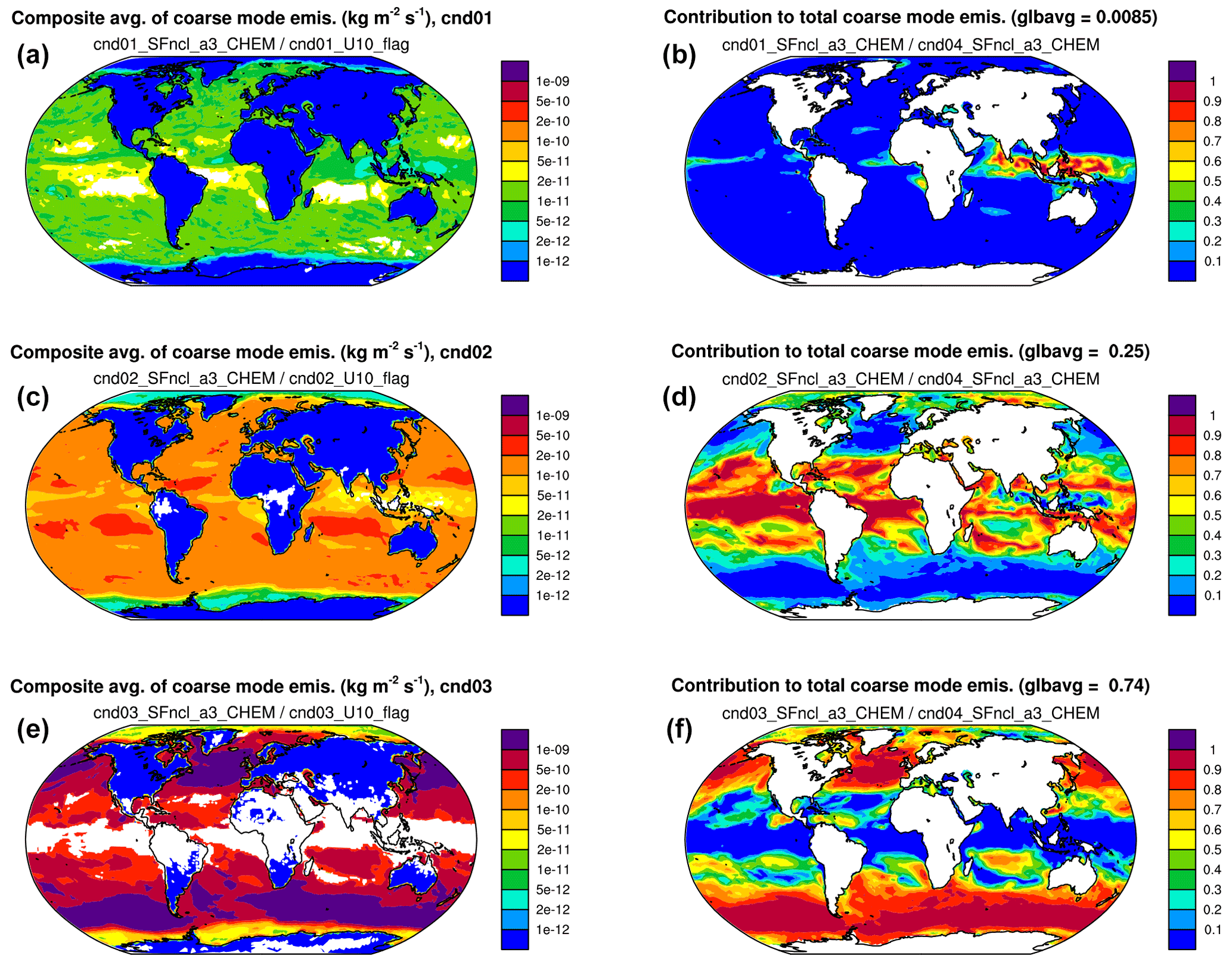
Figure 8(a, c, e) Composite average of coarse-mode sea salt mass emission fluxes under conditions 1–3 corresponding to 10 m wind speed <5 m s−1 (a, b), between 5 and 10 m s−1 (c, d), and >10 m s−1 (e, f). (b, d, f) Contribution of each condition (1, 2, or 3) to the total coarse-mode sea salt emission (condition 4). White areas in the left panels are missing values caused by zero frequency of occurrence of the corresponding conditions. White areas in the right panels are missing values caused by zero total coarse-mode sea salt emission. The expressions given below panel titles indicate how the presented quantities are calculated from the model's output variables.
6.2.1 Simulation setup
In EAMv1, the emission of sea salt aerosol is parameterized with a scheme from Mårtensson et al. (2003) in which the emission flux is proportional to (U10)3.41, with U10 being the wind speed (unit: m s−1) at 10 m above sea level (Zhang et al., 2016; Liu et al., 2012).
Four conditions are specified in the namelist setup shown in Table 3. The first three divide the possible 10 m wind speed values into three ranges: lower than 5 m s−1, between 5 and 10 m s−1, and higher than 10 m s−1. The fourth condition uses the always-fulfilled criterion of U10 > −1 m s−1 to select all grid points and time steps for comparison.
Three QoIs are monitored: SFncl_a1, SFncl_a2, and SFncl_a3, which are the surface mass fluxes of sea salt aerosol in the accumulation mode, Aitken mode, and coarse mode, respectively. These variable names are EAMv1's standard tracer flux names.
U10 in EAMv1 is the grid box average provided by
the coupler (checkpoint MCTCPL).
The calculation of sea salt emissions is done in the atmosphere model
(checkpoint CHEMEMIS).
U10 and the surface fluxes are calculated only once
per time step ΔtCPLmain, and their values remain
available as components of the derived-type Fortran variable
called cam_in (see Table A1).
Therefore,
as long as we select any checkpoint at or after MCTCPL for assessing U10
combined with any checkpoint at or after CHEMEMIS
and before MCTCPL for monitoring the surface fluxes,
the results will be equivalent.
In Table 3, the same checkpoint CHEM is
used for both namelist parameters
cnd_eval_chkpt and
qoi_chkpt, as this is the checkpoint
right before the surface fluxes are used to update
aerosol tracer mixing ratios.
For output, variables from our tool are included in the h0 file as monthly averages.
6.2.2 Results
Figure 7 presents geographical distributions of the frequency of occurrence of conditions 1–3 in the 1-month simulation (left column) and the corresponding composite averages of U10 (right column). While composite averages of U10 are shown for a sanity check, the left panels indicate the different characteristic wind speed associated with different surface types (land versus ocean) and cloud regimes (e.g., deep convection active regions, trade cumulus regions, and storm tracks).
Figure 8 shows geographical distributions of the composite mean of the coarse-mode sea salt mass emission fluxes under conditions 1–3 (left column) and the relative contribution of each condition to the total (all-condition) fluxes (right column). Here, for demonstration purposes, we only chose three wind speed bins and monitored sea salt mass fluxes. If one refines the wind speed ranges (e.g., use 10 to 20 bins), adds aerosol number fluxes to the QoIs, and adds the calculation of global averages to post-processing, then diagrams like Fig. 5 in Zhang et al. (2012) can be created to investigate the simulated relationship between wind speed and particle size distribution of the emissions but without having to write out a large amount of instantaneous model output.
6.3 A conditional budget analysis for RHI
The third example demonstrates a combined use of the budget analysis and conditional sampling capabilities using our tool. The example also requires the calculation of a diagnosed quantity (the relative humidity with respect to ice, RHI) that is not a state variable, so additional routines are invoked to calculate it. This quantity would vary before and after code compartments (e.g., atmospheric dynamics, cloud microphysics, radiation) that operate on the atmospheric state, so it is sensitive to how and where it is calculated in the model, and its value can also change across the subcycles used for the parameterizations and their coupling.
Table 4 Namelist variables pertaining to the new diagnostic tool used in the conditional RHI budget analysis presented in Sect. 6.3.
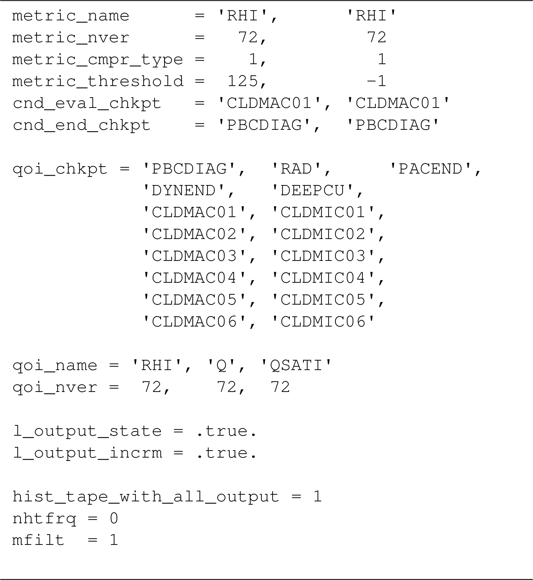
Table 5 For the conditional RHI budget example presented in Sect. 6.3: atmospheric processes corresponding to increments diagnosed at the checkpoints selected in Table 4.

6.3.1 Simulation setup
The focus QoI in this example is
the relative humidity with respect to ice (RHI),
which directly affects the formation of new ice crystals.
In EAMv1, ice nucleation is calculated after the parameterization
of turbulence, shallow convection, and large-scale condensation
represented by
CLUBB (Cloud Layers Unified By Binormals, Golaz et al., 2002; Larson et al., 2002; Larson and Golaz, 2005; Larson, 2017).
CLUBB, ice nucleation, droplet nucleation, and other stratiform
cloud microphysical processes represented by the parameterization
of Gettelman and Morrison (2015) are collectively subcycled
six times per ΔtCPLmain.
Therefore, in the namelist setup shown in Table 4,
a checkpoint is selected before each invocation of the ice nucleation
parameterization (CLDMAC01, …, CLDMAC06) to identify
sources of high RHI.
Additional checkpoints are selected after each invocation of
the stratiform cloud microphysics
(CLDMIC01, …, CLDMIC06)
to monitor how RHI decreases due to those processes.
A few other checkpoints are also selected to evaluate the impact of
atmospheric processes that are known to affect air temperature
and specific humidity, for example large-scale dynamics,
radiation, and deep convection.
In addition to monitoring RHI, we include
the specific humidity (Q) and the saturation specific
humidity with respect to ice (QSATI) as QoIs to
help attribute the diagnosed RHI changes
(see namelist variable qoi_name in Table 4).
While Q is one of the prognostic variables in EAMv1,
RHI and QSATI need to be diagnosed at each checkpoint
using three components of the model's prognostic state:
Q, air temperature, and pressure. The diagnostic subroutines
are included in the module misc_diagnostics.
All of the selected QoIs are
3D variables defined in 72 layers in EAMv1.
Unlike in the previous example, qoi_x_dp is not specified
here; it gets default values of zero, and
therefore no vertical integrals are calculated for the QoIs.
Two sampling conditions are specified: the first one selects grid cells wherein RHI seen by the first invocation of the ice nucleation parameterization is higher than 125 %, which is a necessary although insufficient condition to trigger homogeneous ice nucleation. (For clarification, we note that RHI discussed here is the relative humidity calculated from the grid box mean specific humidity and grid box mean air temperature. EAMv1 uses RHI > RH0 as a screening condition to determine if homogeneous ice nucleation can occur in a grid box. RH0 depends on air temperature but has typical values around 125 %.)
The second condition effectively selects all grid cells and time steps,
but we state the condition as RHI > −1 % instead of using the special
metric ALL and select the same condition-evaluation checkpoint
as in condition 1 so that the conditionally sampled metric
cnd01_RHI and unconditionally sampled cnd02_RHI
can be directly and conveniently compared.
(Using the special metric ALL would result in a metric variable
cnd02_ALL, which is a constant field of 1.0,
being written to the output files.)
The checkpoint before the radiation
parameterization is considered
the end of a full model time step, and hence
cnd_end_chkpt is set to PBCDIAG.
Both the field values and increments of the QoIs are monitored
and included in model output.
The full set of fields tracked by our tool is sent to
output tape 1 (the h0 file), which contains the monthly averages.
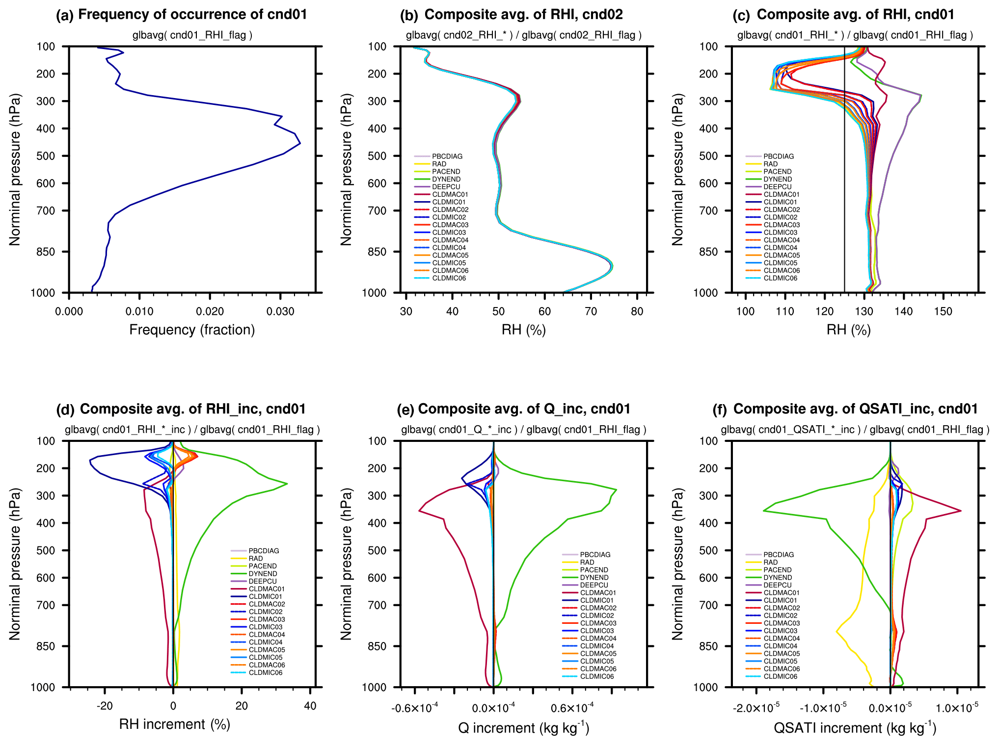
Figure 9(a) The frequency of occurrence of RHI > 125 % averaged over 1 month and the entire globe. (b) RHI at various checkpoints averaged over all time steps of the month and over the entire globe (i.e., RHI under condition 2 – unconditional sampling). (c) Space-and-time mean RHI at various checkpoints under condition 1 (i.e., RHI is higher than 125 % before the first ice nucleation calculation during a time step of ΔtCPLmain=30 min). Space-and-time mean increments of (d) RHI, (e) specific humidity, and (f) saturation specific humidity with respect ice averaged under condition 1.
6.3.2 Results
Figure 9 shows various vertical profiles derived from the simulation. Defining a 2D global average as the average over all grid cells on a sphere weighted by their spherical area, panel (a) in Fig. 9 shows the vertical profile of the 2D global average of the output variable cnd01_RHI_flag, which gives the globally and temporally averaged frequency of occurrence of RHI > 125 % in each grid layer. The other panels in the figure are global averages of different QoIs and checkpoints divided by the global mean frequency of occurrence of the corresponding condition. Recall that our tool assigns a fill value of zero to grid cells and time steps that are unselected for a sampling condition. The profiles in Fig. 9b–f are therefore spatial and temporal averages of the corresponding composites.
Panels (b) and (c) show RHI profiles under conditions 2 and 1, respectively. Sampling using the criterion of RHI > 125 % helps to highlight the substantial changes related to ice cloud formation in the upper troposphere. Panel (d) shows the increments of RHI at various checkpoints, allowing for a direct comparison of the signs and magnitudes of RHI changes caused by different physical processes. The increments of specific humidity and saturation specific humidity shown in panels (e) and (f) can further help to understand the physical mechanisms causing the RHI changes.
An online diagnostic tool has been designed for and implemented in the global atmospheric circulation model EAMv1. The motivation is to introduce a systematic way to support conditional sampling and budget analysis in EAM simulations so as to (1) minimize the need for tedious ad hoc coding, and hence save code development time and avoid clutter, and to (2) reduce the need for instantaneous model output and hence improve the computational efficiency of EAM simulations in which composite or budget analysis is needed.
Building upon the sequential splitting method used by EAM's time integration and the flexibility of the model's output functionalities, the new tool adds its own data structures and functionalities to allow the users to select sampling conditions and model variables (also referred to as quantities of interest, QoIs) to monitor at desired locations of the model's time integration cycles. The condition metrics and QoIs can be any physical quantities that are components of EAM's existing derived-type data structures such as the physics state, physics buffer, and the data structures used for information exchanges between the atmosphere and the surface models such as land and ocean. The condition metrics and QoIs can also be any physical quantities that can be diagnosed from components of these existing data structures. Both the evolving values of the QoIs and their increments caused by different atmospheric processes can be monitored and written out as instantaneous or time-averaged values in EAM's output files (also known as history tapes). For QoIs defined at midpoints of the model's vertical grid or as layer averages, the tool also provides the functionality to calculate and output vertical integrals weighted by the mass of dry or moist air. Multiple sampling conditions can be used in a single simulation. Unconditional sampling and mixtures of conditional and unconditional sampling are also supported.
Assuming the user-chosen conditional metrics and QoIs as well as the locations in time integration cycle to monitor these quantities (referred to as checkpoints) are known to the tool, carrying out a composite or budget analysis using the new tool only requires setting a small number of namelist parameters. The addition of new conditional metrics, QoIs, and checkpoints is straightforward if the data to be sampled can be assessed through EAM's existing data structures.
The new tool has been designed for and implemented in EAMv1 and can be easily ported to EAMv1's descendants (e.g., EAMv2) or predecessors (e.g., CAM5) that use similar Fortran data structures and time integration strategies. Details of the design concepts and implementation in EAMv1 are explained in the paper together with three use case examples that demonstrate the usage of the tool.
The development of the new tool was motivated by the need to carry out conditional budget analysis to understand sources of time step sensitivities and time stepping errors related to EAMv1's physics parameterizations. While the current version of the tool, CondiDiag1.0, fulfills the authors' initial needs in those investigations, we are aware of several aspects in which the tool can be further extended or improved to benefit a wider range of EAM users.
First, if the desired condition metric or QoI is calculated by a lower-level (in software sense) subroutine and is not saved in EAM's derived-type data structures (e.g., physics state, physics buffer), the most convenient way to pass data to CondiDiag will be adding the desired physical quantity to the physics buffer. Such cases will be further assessed and alternative methods will be explored. It is worth noting, however, that the E3SM project has been developing a brand new code base for its version 4 release. The new code uses a single “field manager” for information exchanges between the host model and any resolved or parameterized atmospheric processes. The implementation of our tool in the new code base should make use of – and will benefit from – this new field manager.
Second, the specification of a sampling condition in CondiDiag1.0 takes the form of a logical expression involving the comparison of a single metric with a threshold value. Section 6.2 demonstrates how the tool can be used for a univariate probability distribution analysis. It will be useful to further extend the tool to support sampling conditions involving multiple metrics and a series of threshold values for each metric, hence facilitating multivariate probability distribution analysis. Along that line, it might be useful to support sampling conditions involving multiple metrics evaluated at different checkpoints. This could be useful for investigating forcing-response relationships of multiple atmospheric processes and for evaluating the behavior of subcycled code compartments.
Third, for simulations that involve multiple sampling conditions, the current tool monitors the same set of QoIs and checkpoints under all conditions. It will be useful to provide the flexibility to select different QoIs and checkpoints for different conditions.
Beyond the three aspects discussed above, there are some desirable extensions of the tool that will require more substantial revisions of the current design. For example, in CondiDiag1.0, the sampling conditions are re-evaluated (and the QoIs are resampled) every model time step. We can, however, imagine cases in which a user might want to evaluate a condition at some point of a simulation and monitor the evolution of the atmospheric state in the selected grid cells for longer time periods such as a few hours or a few days. Supporting such use cases will require introducing an additional mechanism to specify how long the evaluated sampling condition is valid. Furthermore, anticipating possible modifications to the sequential splitting of atmospheric processes in EAMv1, in particular possible future adoption of parallel splitting or hybrid methods, it will be useful to explore how the current design of CondiDiag can be extended to accommodate other process-coupling methods.
Tables A1–A3 list the currently available physical quantities that can be used as metrics for conditional sampling or monitored as QoIs.
Table A1Candidate condition metrics and QoIs that
are directly copied from EAM's derived-type data structures.
“<cnst_name>” refers to tracer names in EAM.
“SF<cnst_name>” refers to variable names of
tracer surface fluxes in EAM.
pver and pverp are EAM's variable names
for the number of vertical layers and vertical interfaces, respectively.
In the standard EAMv1, pver is 72 and pverp is 73.
The rightmost column explains the Fortran derived-type variables
and their components from which a metric or QoI's values
are obtained.
More candidate metrics and QoIs can be added following the example shown
by the first code snippet
in Sect. 4.1.2.

Table A2Candidate condition metrics and QoIs that
are directly copied from EAM's “physics buffer” data structure.
pver and pverp are EAM's variable names
for the number of vertical layers and layer interfaces, respectively.
In the standard v1 model, pver is 72 and pverp is 73.
More candidate metrics and QoIs can be added following existing
examples in subroutine get_values in module conditional_diag_main.
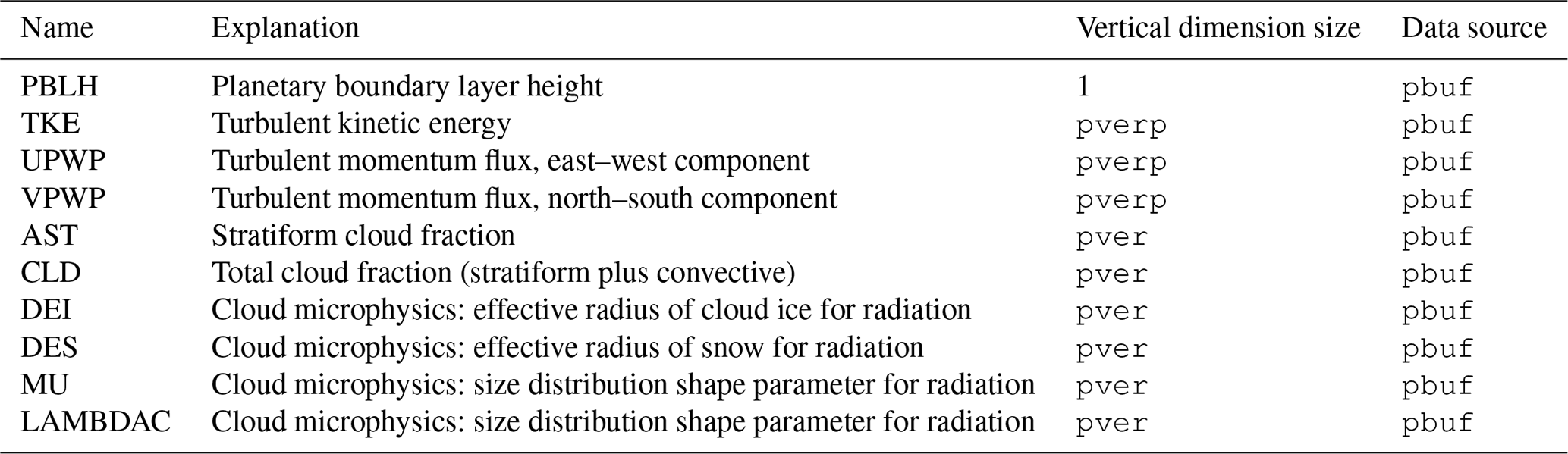
Table A3Candidate condition metrics and QoIs
that are diagnosed from components of EAM's derived-type
data structures.
pver and pverp are EAM's variable names
for the number of vertical layers and vertical interfaces, respectively.
In the standard v1 model, pver is 72 and pverp is 73.
“Subroutine name” is the name of the subroutine in module
misc_diagnostics that calculates the requested quantity.
More candidates can be added following the
the second code snippet in Sect. 4.1.2.
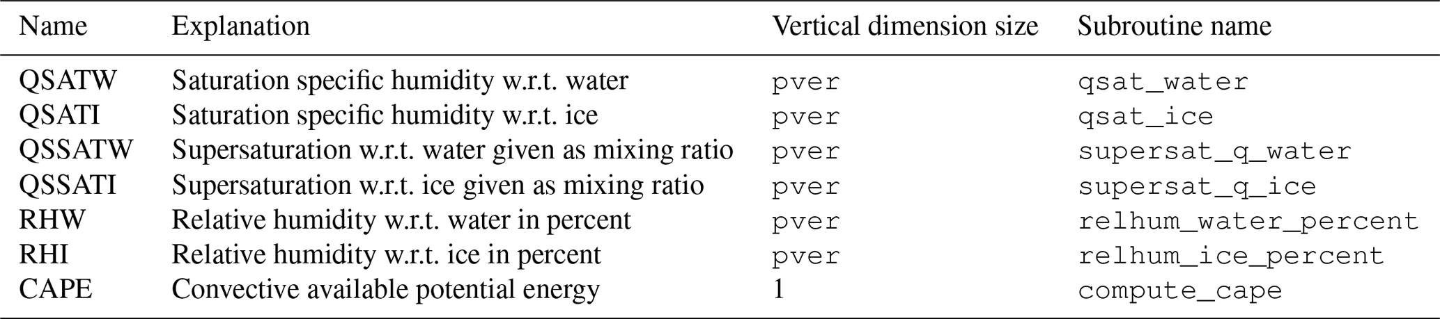
Tables B1 and B2 list
checkpoints currently implemented in EAM's physics driver subroutines
tphysbc and tphysac.
Table B3 lists
the checkpoints in the interface subroutine clubb_tend_cam.
Table B1Checkpoints in the parameterization suite calculated before
coupling with surface models, i.e., in the tphysbc subroutine.
The order of checkpoints in the table is the same as the actual order
of the checkpoints in the code.
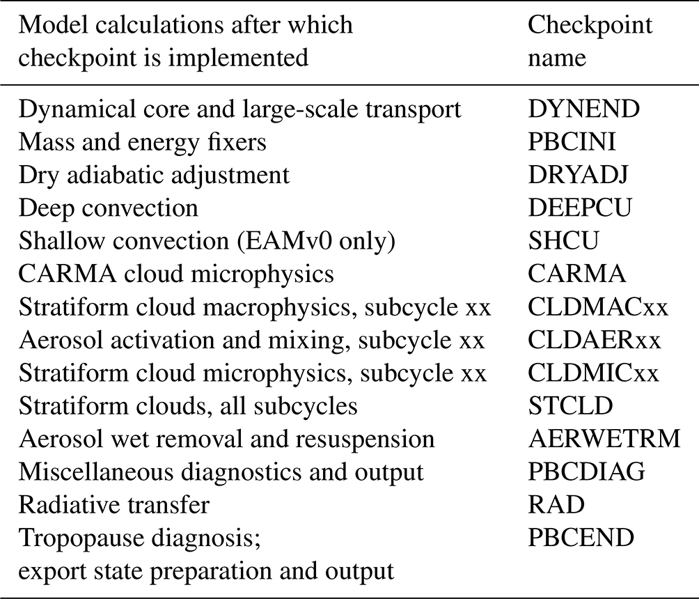
Table B2Checkpoints in the parameterization suite calculated
after coupling with surface models, i.e., in the tphysac subroutine.
The order of checkpoints in the table is the same as the actual order
of the checkpoints in the code.
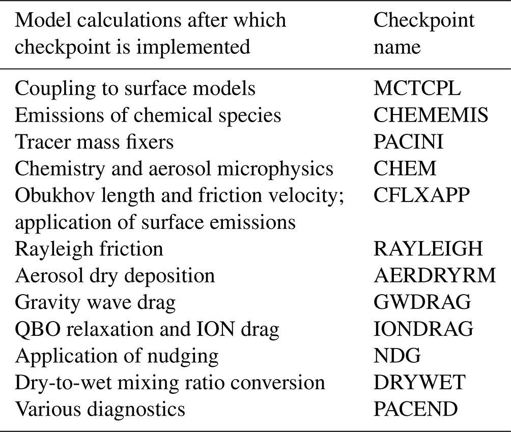
Table B3Checkpoints implemented in the “clubb_tend_cam” subroutine. The order of checkpoints in the table is the same as the actual order of the checkpoints in the code.
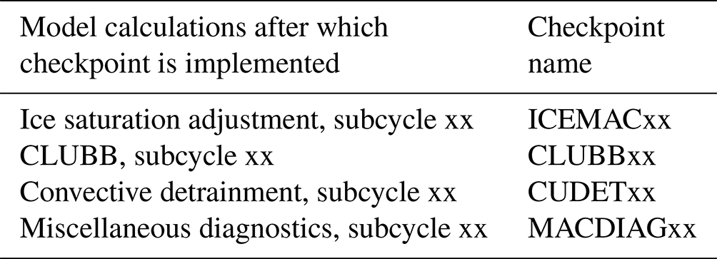
For aerosol and chemical gases which have a dry-to-wet
mixing ratio conversion close to the end of tphysac
(i.e., before the resolved dynamics and transport), a user might want to track the mixing
ratios before and after the conversion as well as
at some other checkpoints. In order to inform our
tool to use the appropriate air mass for the calculation of
vertical integral, an integer array chkpt_x_dp
is included in the namelist conditional_diag_nl.
The values of chkpt_x_dp need to be specified in
relation to qoi_chkpt, i.e.,
one value of chkpt_x_dp for each checkpoint.
A value of 1 tells our tool the mass of moist air
should be used, while a value of 2 indicates dry air mass should be used.
Any other values assigned to chkpt_x_dp
will be interpreted as no specification.
The specifications saved in chkpt_x_dp
are used by our tool when the namelist parameter
qoi_x_dp introduced in Sect. 5.2.4
is assigned values larger than 100.
If a value of 101 (moist) or 102 (dry) is specified for an element of
the array qoi_x_dp,
then the corresponding air mass will be used for that QoI
at all active checkpoints except where
chkpt_x_dp indicates a different specification.
For example, let us assume
we set qoi_x_dp = 102
for the coarse-mode dust mass mixing ratio;
we choose to monitor checkpoints A, B, and C
and set chkpt_x_dp = 0,0,1.
Then, when our tool calculates the coarse-mode dust burden,
checkpoints A and B will use the dry air mass as weights
(because chkpt_x_dp = 0 for these two checkpoints
means no special treatment, while mod(qoi_x_dp,100) = 2
for the QoI means dry air mass should be used).
For checkpoint C, since qoi_x_dp = 102 > 100
and since chkpt_x_dp = 1 for the checkpoint,
the value 1 from chkpt_x_dp will take precedence over
mod(qoi_x_dp,100) = 2, and hence
the moist air mass will be used.
In other words, a value of qoi_x_dp larger than 100
means using mod(qoi_x_dp,100) in general but giving chkpt_x_dp
precedence when the latter is set to nonzero at a checkpoint.
We acknowledge that the description above is likely not easy to
comprehend. For most studies involving vertical integrals of
aerosol or chemical gases, we recommend not
using the checkpoints DRYWET and PACEND listed
in Table B2. By doing that,
the user will get tracer mixing ratios with consistent definitions
at all checkpoints so that only qoi_x_dp (with values 0, 1, or 2)
is needed for turning on or off the vertical integral.
Last but not least, we clarify that mixing ratios of water species do not have this conversion problem.
The EAMv1 code, run scripts, and post-processing scripts used in this paper can be found on Zenodo at https://doi.org/10.5281/zenodo.6325126 (Wan et al., 2022). Two versions of the EAM maint-1.0 code are provided: one with CondiDiag1.0 implemented and one without, both of which can be compiled and run on E3SM's supported computer systems. The Zenodo archive also provides a third, smaller tar ball which contains only the source files that were added or revised during the implementation of CondiDiag1.0. A copy of the corresponding EAMv1 files before the implementation is included in this third tar ball to facilitate comparison.
The simulation output files of the three use case examples shown in Sect. 6 can be found on Zenodo under https://doi.org/10.5281/zenodo.6451952 (Wan and Zhang, 2022).
HW designed and implemented CondiDiag in EAMv1 with feedback from the coauthors. KZ and HW designed the use case examples. HW carried out the simulations and processed the results. HW wrote the paper; all coauthors helped with the revisions.
The contact author has declared that neither they nor their coauthors have any competing interests.
Publisher's note: Copernicus Publications remains neutral with regard to jurisdictional claims in published maps and institutional affiliations.
We thank the two anonymous reviewers and Sean Santos for their constrictive comments, which helped to improve the paper. Cecile Hannay at NCAR is thanked for her help with various versions and formats of CAM's documentation. Computing resources for the initial development and testing of the new tool were provided by the National Energy Research Scientific Computing Center (NERSC), a US Department of Energy (DOE) Office of Science User Facility supported by the Office of Science of the US Department of Energy under contract no. DE-AC02-05CH11231.
Simulations shown as use case examples in this paper were carried out using the DOE Biological and Environmental Research (BER) Earth System Modeling program's Compy computing cluster located at Pacific Northwest National Laboratory (PNNL). PNNL is operated by the Battelle Memorial Institute for the US Department of Energy under contract DE-AC05-76RL01830.
The EAMv1 code was obtained from the E3SM project sponsored by DOE BER (https://doi.org/10.11578/E3SM/dc.20180418.36, E3SM, 2018).
This research was supported by DOE BER via the Scientific Discovery through Advanced Computing (SciDAC) program (grant no. 70276). KZ was supported by DOE BER through the E3SM project (grant no. 65814).
This paper was edited by Axel Lauer and reviewed by two anonymous referees.
Bailey, A., Singh, H. K. A., and Nusbaumer, J.: Evaluating a Moist Isentropic Framework for Poleward Moisture Transport: Implications for Water Isotopes Over Antarctica, Geophys. Res. Lett., 46, 7819–7827, https://doi.org/10.1029/2019GL082965, 2019. a
Craig, A. P., Vertenstein, M., and Jacob, R.: A new flexible coupler for earth system modeling developed for CCSM4 and CESM1, Int. J. High Perform. C., 26, 31–42, https://doi.org/10.1177/1094342011428141, 2012. a
Craig, C., Bacmeister, J., Callaghan, P., Eaton, B., Gettelman, A., Goldhaber, S. N., Hannay, C., Herrington, A., Lauritzen, P. H., McInerney, J., Medeiros, B., Mills, M. J., Neale, R., Tilmes, S., Truesdale, J. E., Vertenstein, M., and Vitt, F. M.: CAM6.3 User's Guide, NCAR Technical Note NCAR/TN-571+EDD, National Center for Atmospheric Research, Boulder, Colorado, USA, https://doi.org/10.5065/Z953-ZC95, 2021. a, b
E3SM Project: Energy Exascale Earth System Model v1.0 [code], https://doi.org/10.11578/E3SM/dc.20180418.36, 2018. a
Eaton, B.: CAM Reference Manual, https://www.cesm.ucar.edu/models/cesm1.2/cam/docs/rm5_3/index.html (last access: 13 April 2022), 2015. a, b
Gettelman, A. and Morrison, H.: Advanced two-moment bulk microphysics for global models, Part I: Off-line tests and comparison with other schemes, J. Climate, 28, 1268–1287, https://doi.org/10.1175/JCLI-D-14-00102.1, 2015. a
Ghan, S., Wang, M., Zhang, S., Ferrachat, S., Gettelman, A., Griesfeller, J., Kipling, Z., Lohmann, U., Morrison, H., Neubauer, D., Partridge, D., Stier, P., Takemura, T., Wang, H., and Zhang, K.: Challenges in constraining anthropogenic aerosol effects on cloud radiative forcing using present-day spatiotemporal variability, P. Natl. Acad. Sci. USA, 113, 5804–5811, 2016. a
Golaz, J.-C., Larson, V., and Cotton, W.: A PDF-Based Model for Boundary Layer Clouds. Part I: Method and Model Description, J. Atmos. Sci., 59, 3540–3551, https://doi.org/10.1175/1520-0469(2002)059<3540:APBMFB>2.0.CO;2, 2002. a
Golaz, J.-C., Caldwell, P. M., Van Roekel, L. P., Petersen, M. R., Tang, Q., Wolfe, J. D., Abeshu, G., Anantharaj, V., Asay-Davis, X. S., Bader, D. C., Baldwin, S. A., Bisht, G., Bogenschutz, P. A., Branstetter, M., Brunke, M. A., Brus, S. R., Burrows, S. M., Cameron-Smith, P. J., Donahue, A. S., Deakin, M., Easter, R. C., Evans, K. J., Feng, Y., Flanner, M., Foucar, J. G., Fyke, J. G., Griffin, B. M., Hannay, C., Harrop, B. E., Hoffman, M. J., Hunke, E. C., Jacob, R. L., Jacobsen, D. W., Jeffery, N., Jones, P. W., Keen, N. D., Klein, S. A., Larson, V. E., Leung, L. R., Li, H.-Y., Lin, W., Lipscomb, W. H., Ma, P.-L., Mahajan, S., Maltrud, M. E., Mametjanov, A., McClean, J. L., McCoy, R. B., Neale, R. B., Price, S. F., Qian, Y., Rasch, P. J., Reeves Eyre, J. E. J., Riley, W. J., Ringler, T. D., Roberts, A. F., Roesler, E. L., Salinger, A. G., Shaheen, Z., Shi, X., Singh, B., Tang, J., Taylor, M. A., Thornton, P. E., Turner, A. K., Veneziani, M., Wan, H., Wang, H., Wang, S., Williams, D. N., Wolfram, P. J., Worley, P. H., Xie, S., Yang, Y., Yoon, J.-H., Zelinka, M. D., Zender, C. S., Zeng, X., Zhang, C., Zhang, K., Zhang, Y., Zheng, X., Zhou, T., and Zhu, Q.: The DOE E3SM Coupled Model Version 1: Overview and Evaluation at Standard Resolution, J. Adv. Model. Earth Sy., 11, 2089–2129, https://doi.org/10.1029/2018MS001603, 2019. a, b
Gryspeerdt, E., Mülmenstädt, J., Gettelman, A., Malavelle, F. F., Morrison, H., Neubauer, D., Partridge, D. G., Stier, P., Takemura, T., Wang, H., Wang, M., and Zhang, K.: Surprising similarities in model and observational aerosol radiative forcing estimates, Atmos. Chem. Phys., 20, 613–623, https://doi.org/10.5194/acp-20-613-2020, 2020. a
Larson, V. E.: CLUBB-SILHS: A parameterization of subgrid variability in the atmosphere, arXiv [preprint], arXiv:1711.03675v3, 2017. a
Larson, V. E. and Golaz, J.-C.: Using Probability Density Functions to Derive Consistent Closure Relationships among Higher-Order Moments, Mon. Weather Rev., 133, 1023–1042, https://doi.org/10.1175/MWR2902.1, 2005. a
Larson, V. E., Golaz, J.-C., and Cotton, W. R.: Small-Scale and Mesoscale Variability in Cloudy Boundary Layers: Joint Probability Density Functions, J. Atmos. Sci., 59, 3519–3539, https://doi.org/10.1175/1520-0469(2002)059<3519:SSAMVI>2.0.CO;2, 2002. a
Liu, X., Easter, R. C., Ghan, S. J., Zaveri, R., Rasch, P., Shi, X., Lamarque, J.-F., Gettelman, A., Morrison, H., Vitt, F., Conley, A., Park, S., Neale, R., Hannay, C., Ekman, A. M. L., Hess, P., Mahowald, N., Collins, W., Iacono, M. J., Bretherton, C. S., Flanner, M. G., and Mitchell, D.: Toward a minimal representation of aerosols in climate models: description and evaluation in the Community Atmosphere Model CAM5, Geosci. Model Dev., 5, 709–739, https://doi.org/10.5194/gmd-5-709-2012, 2012. a
Ma, H.-Y., Xie, S., Boyle, J. S., Klein, S. A., and Zhang, Y.: Metrics and Diagnostics for Precipitation-Related Processes in Climate Model Short-Range Hindcasts, J. Climate, 26, 1516–1534, https://doi.org/10.1175/JCLI-D-12-00235.1, 2013. a
Ma, H.-Y., Xie, S., Klein, S. A., Williams, K. D., Boyle, J. S., Bony, S., Douville, H., Fermepin, S., Medeiros, B., Tyteca, S., Watanabe, M., and Williamson, D.: On the Correspondence between Mean Forecast Errors and Climate Errors in CMIP5 Models, J. Climate, 27, 1781–1798, https://doi.org/10.1175/JCLI-D-13-00474.1, 2014. a
Mårtensson, E. M., Nilsson, E. D., de Leeuw, G., Cohen, L. H., and Hansson, H.-C.: Laboratory simulations and parameterization of the primary marine aerosol production, J. Geophys. Res.-Atmos., 108, 4297, https://doi.org/10.1029/2002JD002263, 2003. a
Martin, G., Milton, S., Senior, C., Brooks, M., Ineson, S., Reichler, T., and Kim, J.: Analysis and Reduction of Systematic Errors through a Seamless Approach to Modeling Weather and Climate, J. Climate, 23, 5933–5957, https://doi.org/10.1175/2010JCLI3541.1, 2010. a
Neale, R. B., Richter, J. H., Conley, A. J., Park, S., Lauritzen, P. H., Gettelman, A., Williamson, D. L., Rasch, P. J., Vavrus, S. J., Taylor, M. A., Collins, W. D., Zhang, M., and Lin, S.-J.: Description of the NCAR Community Atmosphere Model (CAM4.0), NCAR Technical Note NCAR/TN-485+STR, National Center for Atmospheric Research, Boulder, Colorado, USA, http://www.cesm.ucar.edu/models/ccsm4.0/cam/docs/description/cam4_desc.pdf (last access: 13 April 2022), 2010. a
Neale, R. B., Chen, C. C., Gettelman, A., Lauritzen, P. H., Park, S., Williamson, D. L., Conley, A. J., Garcia, R., Kinnison, D., Lamarque, J. F., Marsh, D., Mills, M., Smith, A. K., Tilmes, S., Vitt, F., Morrison, H., Cameron-Smith, P., Collins, W. D., Iacono, M. J., Easter, R. C., Ghan, S. J., Liu, X. H., Rasch, P. J., and Taylor, M. A.: Description of the NCAR Community Atmosphere Model (CAM5.0), NCAR Technical Note NCAR/TN-486+STR, National Center for Atmospheric Research, Boulder, Colorado, USA, https://www.cesm.ucar.edu/models/cesm1.0/cam/docs/description/cam5_desc.pdf (last access: 13 April 2022), 2012. a
Phillips, T. J., Potter, G. L., Williamson, D. L., Cederwall, R. T., Boyle, J. S., Fiorino, M., Hnilo, J. J., Olson, J. G., Xie, S., and Yio, J. J.: Evaluating Parameterizations in General Circulation Models: Climate Simulation Meets Weather Prediction, B. Amer. Meteorol. Soc., 85, 1903–1916, https://doi.org/10.1175/BAMS-85-12-1903, 2004. a
Rasch, P. J., Xie, S., Ma, P.-L., Lin, W., Wang, H., Tang, Q., Burrows, S. M., Caldwell, P., Zhang, K., Easter, R. C., Cameron-Smith, P., Singh, B., Wan, H., Golaz, J.-C., Harrop, B. E., Roesler, E., Bacmeister, J., Larson, V. E., Evans, K. J., Qian, Y., Taylor, M., Leung, L. R., Zhang, Y., Brent, L., Branstetter, M., Hannay, C., Mahajan, S., Mametjanov, A., Neale, R., Richter, J. H., Yoon, J.-H., Zender, C. S., Bader, D., Flanner, M., Foucar, J. G., Jacob, R., Keen, N., Klein, S. A., Liu, X., Salinger, A., Shrivastava, M., and Yang, Y.: An Overview of the Atmospheric Component of the Energy Exascale Earth System Model, J. Adv. Model. Earth Sy., 11, 2377–2411, https://doi.org/10.1029/2019MS001629, 2019. a
Richter, J. H. and Rasch, P. J.: Effects of Convective Momentum Transport on the Atmospheric Circulation in the Community Atmosphere Model, Version 3, J. Clim., 21, 1487–1499, https://doi.org/10.5194/gmd-10-2221-2017, 2008. a
Singh, H. A., Bitz, C. M., Nusbaumer, J., and Noone, D. C.: A mathematical framework for analysis of water tracers: Part 1: Development of theory and application to the preindustrial mean state, J. Adv. Model. Earth Sy., 8, 991–1013, https://doi.org/10.1002/2016MS000649, 2016. a
Wan, H. and Zhang, K.: EAMv1 simulation output from CondiDiag1.0 use case examples, Zenodo [data set], https://doi.org/10.5281/zenodo.6451952, 2022. a
Wan, H., Zhang, S., Rasch, P. J., Larson, V. E., Zeng, X., and Yan, H.: Quantifying and attributing time step sensitivities in present-day climate simulations conducted with EAMv1, Geosci. Model Dev., 14, 1921–1948, https://doi.org/10.5194/gmd-14-1921-2021, 2021. a, b
Wan, H., Zhang, K., and Rasch, P. J.: CondiDiag1.0 implemented in EAMv1, Zenodo [code], https://doi.org/10.5281/zenodo.6325126, 2022. a, b
Wang, H., Rasch, P. J., Easter, R. C., Singh, B., Zhang, R., Ma, P.-L., Qian, Y., Ghan, S. J., and Beagley, N.: Using an explicit emission tagging method in global modeling of source-receptor relationships for black carbon in the Arctic: Variations, sources, and transport pathways, J. Geophys. Res.-Atmos., 119, 12888–12909, https://doi.org/10.1002/2014JD022297, 2014. a
Wang, H., Fyke, J. G., Lenaerts, J. T. M., Nusbaumer, J. M., Singh, H., Noone, D., Rasch, P. J., and Zhang, R.: Influence of sea-ice anomalies on Antarctic precipitation using source attribution in the Community Earth System Model, The Cryosphere, 14, 429–444, https://doi.org/10.5194/tc-14-429-2020, 2020. a
Williams, K. D., Bodas-Salcedo, A., Déqué, M., Fermepin, S., Medeiros, B., Watanabe, M., Jakob, C., Klein, S. A., Senior, C. A., and Williamson, D. L.: The Transpose-AMIP II Experiment and Its Application to the Understanding of Southern Ocean Cloud Biases in Climate Models, J. Climate, 26, 3258–3274, https://doi.org/10.1175/JCLI-D-12-00429.1, 2013. a
Williamson, D. L., Boyle, J., Cederwall, R., Fiorino, M., Hnilo, J., Olson, J., Phillips, T., Potter, G., and Xie, S. C.: Moisture and temperature balances at the Atmospheric Radiation Measurement Southern Great Plains Site in forecasts with the Community Atmosphere Model (CAM2), J. Geophys. Res., 110, 1–17, https://doi.org/10.1029/2004JD005109, 2005. a
Xie, S., Ma, H.-Y., Boyle, J. S., Klein, S. A., and Zhang, Y.: On the Correspondence between Short- and Long-Time-Scale Systematic Errors in CAM4/CAM5 for the Year of Tropical Convection, J. Climate, 25, 7937–7955, https://doi.org/10.1175/JCLI-D-12-00134.1, 2012. a
Xie, S., Lin, W., Rasch, P. J., Ma, P., Neale, R., Larson, V. E., Qian, Y., Bogenschutz, P. A., Caldwell, P., Cameron?Smith, P., Golaz, J., Mahajan, S., Singh, B., Tang, Q., Wang, H., Yoon, J., Zhang, K., and Zhang, Y.: Understanding cloud and convective characteristics in version 1 of the E3SM atmosphere model, J. Adv. Model. Earth Sy., 10, 2618–2644, https://doi.org/10.1029/2018MS001350, 2018. a
Zhang, G. J. and McFarlane, N. A.: Sensitivity of climate simulations to the parameterization of cumulus convection in the Canadian Climate Centre general circulation model, Atmos. Ocean, 33, 407–446, https://doi.org/10.1080/07055900.1995.9649539, 1995. a
Zhang, K., O'Donnell, D., Kazil, J., Stier, P., Kinne, S., Lohmann, U., Ferrachat, S., Croft, B., Quaas, J., Wan, H., Rast, S., and Feichter, J.: The global aerosol-climate model ECHAM-HAM, version 2: sensitivity to improvements in process representations, Atmos. Chem. Phys., 12, 8911–8949, https://doi.org/10.5194/acp-12-8911-2012, 2012. a
Zhang, K., Zhao, C., Wan, H., Qian, Y., Easter, R. C., Ghan, S. J., Sakaguchi, K., and Liu, X.: Quantifying the impact of sub-grid surface wind variability on sea salt and dust emissions in CAM5, Geoscientific Model Development, 9, 607–632, https://doi.org/10.5194/gmd-9-607-2016, 2016. a
Zhang, K., Rasch, P. J., Taylor, M. A., Wan, H., Leung, R., Ma, P.-L., Golaz, J.-C., Wolfe, J., Lin, W., Singh, B., Burrows, S., Yoon, J.-H., Wang, H., Qian, Y., Tang, Q., Caldwell, P., and Xie, S.: Impact of numerical choices on water conservation in the E3SM Atmosphere Model version 1 (EAMv1), Geosci. Model Dev., 11, 1971–1988, https://doi.org/10.5194/gmd-11-1971-2018, 2018. a
Zhang, R., Wang, H., Hegg, D. A., Qian, Y., Doherty, S. J., Dang, C., Ma, P.-L., Rasch, P. J., and Fu, Q.: Quantifying sources of black carbon in western North America using observationally based analysis and an emission tagging technique in the Community Atmosphere Model, Atmos. Chem. Phys., 15, 12805–12822, https://doi.org/10.5194/acp-15-12805-2015, 2015. a
- Abstract
- Introduction
- Host model features
- Nomenclature and design concepts for CondiDiag
- Implementation in EAMv1
- User guide
- Use case examples
- Conclusions and outlook
- Appendix A: Candidate metrics and QoIs in CondiDiag1.0
- Appendix B: Checkpoints in CondiDiag1.0
- Appendix C: Additional notes on vertical integrals
- Code availability
- Data availability
- Author contributions
- Competing interests
- Disclaimer
- Acknowledgements
- Financial support
- Review statement
- References