the Creative Commons Attribution 4.0 License.
the Creative Commons Attribution 4.0 License.
 | 17 Jan 2022
BioRT-Flux-PIHM v1.0: a biogeochemical reactive transport model at the watershed scale
Yuning Shi
Leila Saberi
Gene-Hua Crystal Ng
Kayalvizhi Sadayappan
Devon Kerins
Bryn Stewart
Watersheds are the fundamental Earth surface functioning units that connect the land to aquatic systems. Many watershed-scale models represent hydrological processes but not biogeochemical reactive transport processes. This has limited our capability to understand and predict solute export, water chemistry and quality, and Earth system response to changing climate and anthropogenic conditions. Here we present a recently developed BioRT-Flux-PIHM (BioRT hereafter) v1.0, a watershed-scale biogeochemical reactive transport model. The model augments the previously developed RT-Flux-PIHM that integrates land-surface interactions, surface hydrology, and abiotic geochemical reactions. It enables the simulation of (1) shallow and deep-water partitioning to represent surface runoff, shallow soil water, and deeper groundwater and of (2) biotic processes including plant uptake, soil respiration, and nutrient transformation. The reactive transport part of the code has been verified against the widely used reactive transport code CrunchTope. BioRT-Flux-PIHM v1.0 has recently been applied in multiple watersheds under diverse climate, vegetation, and geological conditions. This paper briefly introduces the governing equations and model structure with a focus on new aspects of the model. It also showcases one hydrology example that simulates shallow and deep-water interactions and two biogeochemical examples relevant to nitrate and dissolved organic carbon (DOC). These examples are illustrated in two simulation modes of complexity. One is the spatially lumped mode (i.e., two land cells connected by one river segment) that focuses on processes and average behavior of a watershed. Another is the spatially distributed mode (i.e., hundreds of cells) that includes details of topography, land cover, and soil properties. Whereas the spatially lumped mode represents averaged properties and processes and temporal variations, the spatially distributed mode can be used to understand the impacts of spatial structure and identify hot spots of biogeochemical reactions. The model can be used to mechanistically understand coupled hydrological and biogeochemical processes under gradients of climate, vegetation, geology, and land use conditions.
- Article
(3630 KB) - Full-text XML
-
Supplement
(553 KB) - BibTeX
- EndNote


Watersheds are the fundamental Earth surface units that receive and process water, mass, and energy (Li, 2019; Li et al., 2021; Hubbard et al., 2018). Watershed processes include land-surface interactions that regulate evapotranspiration and discharge as well as water partitioning between shallow soil lateral flow going into streams vs. downward flow and recharge into the deeper subsurface (Fig. 1). Complex biogeochemical interactions occur among soil, water, roots, and microbes along water's flow paths, regulating gas effluxes (e.g., CO2) and solute export (Fatichi et al., 2019; van der Velde et al., 2010; Benettin et al., 2020; Adler et al., 2021).
These hydrological and biogeochemical processes determine how Earth surface systems respond to hydroclimatic forcing and human perturbations. Understanding these processes remains challenging due to the complex process interactions. An example is the concentration–discharge (C–Q) relationships of solutes at stream and river outlets. Similar C–Q relationships have been observed for some solutes across watersheds under distinct geological and climatic conditions (Godsey et al., 2009; Basu et al., 2010; Moatar et al., 2017; Zarnetske et al., 2018; Godsey et al., 2019), whereas different solutes have shown contrasting patterns in the same watershed (Miller et al., 2017; Herndon et al., 2015; Musolff et al., 2015; Stewart et al., 2021; Zhi et al., 2020b). A general theory that can explain contrasting C–Q observations (e.g., flushing vs. dilution behaviors) under diverse watershed characteristics and external conditions remains elusive. The lack of mechanistic understanding presents major roadblocks to forecasting water quality and Earth system dynamics in the future.
One of the outstanding challenges is the lack of modeling tools that mechanistically link hydrological and biogeochemical processes at the watershed scale. Model development has advanced mostly within the disciplinary boundaries of hydrology and biogeochemistry (Li, 2019). Watershed hydrologic models focus on solving for water storage and fluxes (Fatichi et al., 2016). Reactive transport models (RTMs) have traditionally focused on transport and multi-component biogeochemical reactions mostly in groundwater systems with limited interactions with climate and other surficial conditions (Steefel et al., 2015; Li et al., 2017b). Some integration crossing disciplinary boundaries did occur in recent years. For example, SWAT (Soil and Water Assessment Tool) has a version that couples with the groundwater model MODFLOW and the surface water and groundwater quality model in RT3D (Bailey et al., 2017; Ochoa et al., 2020). CATHY (Catchment Hydrology) includes processes of pesticide decay (Gatel et al., 2019; Scudeler et al., 2016). Hydrologiska Byråns Vattenbalansavdelning (HBV) and the Hydrological Predictions for the Environment (HYPE) have modules that simulate processes relevant to nutrients and contaminants (Lindström et al., 2005, 2010). While these models can simulate processes such as leaching of nutrients from agriculture lands (Lindström et al., 2005, 2010; Bailey et al., 2017), they do not explicitly solve the multi-component reactive transport equations. In other words, reactions are often represented rudimentarily without honoring kinetics and thermodynamics theories in soil biogeochemistry and geochemistry. For example, nutrient leaching is calculated based on empirical equations without explicitly solving reactive transport equations. Reaction rates are represented using first-order decay (Gatel et al., 2019), assuming constant reaction rates that do not change with environmental conditions. Biogeochemical processes however are highly variable with seasonal dynamics and depend on local environments such as substrate availability, soil temperature, and soil moisture (Li et al., 2017a; Davidson and Janssens, 2006). These models therefore cannot capture the temporal variations in environmental factors that regulate soil biogeochemical reactions and stream and water chemistry.
To fill this model capability need, we augmented the watershed model RT-Flux-PIHM (Bao et al., 2017) into BioRT-Flux-PIHM (BioRT hereafter). Compared to RT-Flux-PIHM, BioRT has two additions. One is the capability of simulating biotic processes including plant uptake of nutrients, soil respiration, and other microbe-mediated redox reactions. Examples include soil respiration that produces CO2 and dissolved organic carbon (DOC) and nutrient transformation reactions such as nitrification and denitrification. The other is the addition of an optional deeper layer below shallow soil to enable the simulation of interacting deep-water and shallow soil water flow (Fig. 1). Here the deep water is loosely defined as the water below the soil zone, typically in less weathered, fractured subsurface that harbors relatively old and slow-moving groundwater contributing to streams. It is a fundamental component of the hydrologic cycle and water budget. The groundwater–surface-water interactions also modulate land–atmospheric energy exchanges and soil moisture dynamics (Keune et al., 2016). Evidence has been mounting in recent years that deeper water below the shallow soil interacts with streams, introduces water with distinct chemistry, sustains base flow in dry times, and buffers climate variability (Gurdak, 2017; Green, 2016; Taylor et al., 2013). Stream chemistry often reflects distinct chemistry from shallow soil water and deeper groundwater at different times, i.e., the so-called Shallow and Deep Hypothesis (Zhi et al., 2019; Zhi and Li, 2020; Botter et al., 2020). Including the deep-water component thus is essential for understanding mechanisms and predicting dynamics of water quality under changing climate and human conditions.
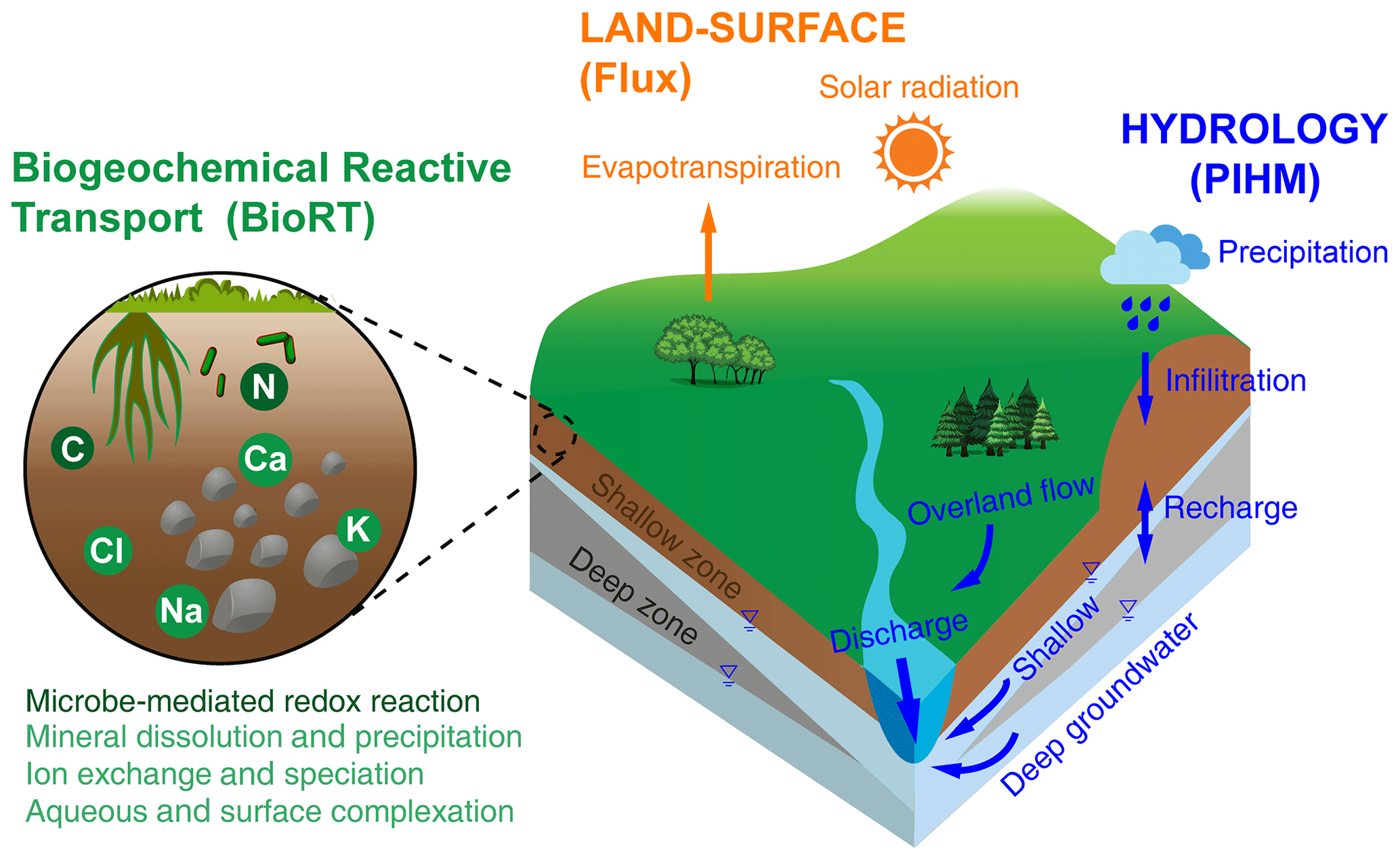
Figure 1A conceptual diagram for processes at the watershed scale. Land-surface interactions include processes such as energy balance, solar radiation, and evapotranspiration; hydrological processes partition water between surface runoff, shallow soil water, and deeper water. Soil biogeochemical reactions include abiotic reactions such as weathering (e.g., mineral dissolution and precipitation, ion exchange, surface complexations) and biotic processes such as plant uptake and leaching of nutrients, soil respiration, and other microbe-mediated reactions. These processes are represented in three modules: the Flux module for land-surface interactions, the PIHM module for catchment hydrology, and the BioRT module for biogeochemical reactions. Conceptually the shallow zone is the shallow soil and weathered zone that is more conductive to water flow (e.g., soil lateral flow or interflow). The deep zone refers to the less weathered zone that often harbors the old and slow-flowing groundwater. Reactions can occur in both shallow and deep zones.
This paper introduces the new developments in BioRT. The paper starts with a brief overview of water- and energy-related processes. It then introduces governing equations and reaction kinetics used in BioRT, followed by three examples that illustrate the new capabilities. The examples include the surface water and groundwater interactions, nitrate transformation and transport, and the production and export of DOC. The model can be set up in both spatially lumped or spatially explicit modes. The source code and the examples here are archived on the Zenodo website (https://doi.org/10.5281/zenodo.3936073) and the GitHub website (https://github.com/Li-Reactive-Water-Group/BioRT-Flux-PIHM, last access: 23 September 2021).
BioRT-Flux-PIHM integrates three modules (Fig. 1). The Flux module is for land-surface processes including surface energy balance, solar radiation, and evapotranspiration (ET) (Shi et al., 2013). The hydrology module PIHM simulates water processes including precipitation, interception, infiltration, recharge, surface runoff, subsurface lateral flow, and deep-water flow (Qu and Duffy, 2007). The BioRT module simulates solute transport and reactions. The abiotic reactions included in RT-Flux-PIHM (Bao et al., 2017) are mineral dissolution and precipitation, aqueous and surface complexation, and ion exchange reactions. The newly added reactions include plant uptake of nutrients, soil respiration, and microbe-mediated redox reactions (e.g., carbon decomposition and nutrient transformation).
The land-surface and hydrology modules solve for soil temperature and water storage, from which water fluxes are calculated for surface runoff and shallow- and deep-water fluxes. The BioRT module uses the calculated soil temperature, water storage, and water fluxes to simulate solute transport (advective and diffusive–dispersive) and biogeochemical reactions in both shallow and deep zones (see governing equations in later sections). The reactions include kinetically controlled (e.g., microbe-mediated redox reaction, mineral dissolution, and precipitation) or equilibrium-controlled ones (e.g., ion exchange, surface complexation (sorption), and aqueous complexation). Users can define the types of reactions to be included and the form of reaction kinetics in input files. The output of BioRT includes the spatial distribution and time series of aqueous and solid concentrations, from which we can infer reaction rates.
The model can be set up running in either spatially lumped or spatially explicit modes. When running in spatially explicit mode, the simulation domain can be structured as prismatic grids based on topography. Each grid is partitioned into surface and shallow and deep subsurface layers. The surface layer calculates water flow above ground (surface runoff). The shallow zone is loosely defined as the highly permeable subsurface that contrasts the deep zone that is broadly defined as the lower permeability zone beyond the shallow zone. In many places, the shallow zone is the soil zone that is most conductive to water flow (e.g., lateral flow) and is responsive to hydroclimatic forcing. The deep subsurface zone is the less weathered layer that harbors the old groundwater that contributes to stream flow. Note that these definitions differ from those in the hydrology community, which often refers to the shallow soil lateral flow as groundwater, in a way that distinguishes it from the surface runoff (Dingman, 2015). These source waters from different depths of the subsurface often have distinct solid and water chemistry and are dominant at different hydrological conditions at different times of the year, as has been observed in many catchments and watersheds (Brantley et al., 2018; Zhi et al., 2019; Zhi and Li, 2020; Sullivan et al., 2016). The model is flexible for taking inputs from online data portals or local measurements, and it can accommodate low data availability (see the following Sect. 5 for data need and domain setup).
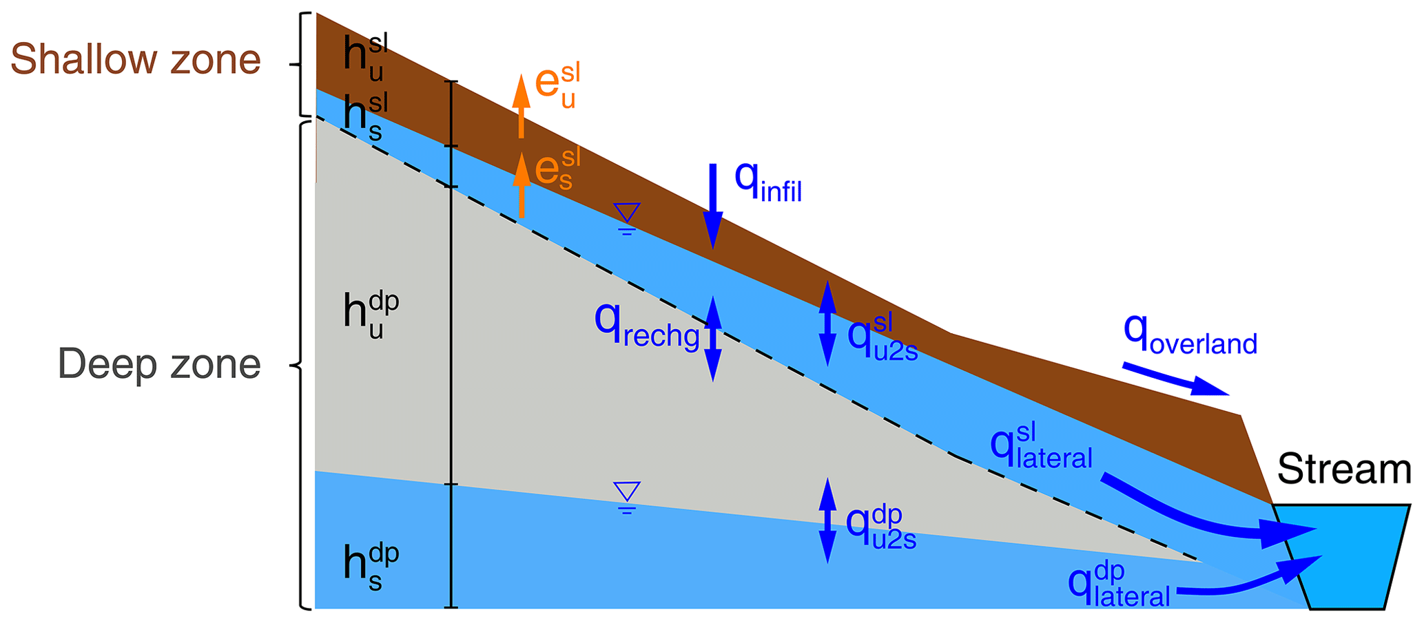
Figure 2Hillslope view of the shallow and deep zones and relevant water flows. Streams received water primarily from three water flows: the surface runoff (qoverland), lateral flow from the shallow zone , and the lateral flow that has been recharged and eventually come out from the deeper zone . The symbols “h”, “e”, and “q” denote water storage, evapotranspiration, and water flow, respectively. The superscript letters “sl” and “dp” refer to shallow and deep zones, respectively. The subscript letters “u” and “s” refer to unsaturated and saturated layers, respectively. Detailed equations are in Sect. 3.1 and 3.2. The terms “infil”, “u2s”, and “recharge” refer to infiltration, unsaturated to saturated zones, and recharge.
3.1 Water equations
Flux-PIHM simulates surface runoff and a lumped subsurface flux into streams without distinguishing shallow soil water and deeper groundwater flow paths. Mounting evidence has shown that the shallow soil water and deeper groundwater have distinct chemistry and are dominant at different times of the year (Xiao et al., 2021; Zhi and Li, 2020; Zhi et al., 2019). This means that a lumped subsurface flow cannot describe the dynamics of stream chemistry. We therefore added a deeper groundwater zone to simulate deeper water flows that interact with streams (Fig. 2). Each prismatic element now has three zones in the vertical direction: surface (or above ground) and shallow and deep zones in the subsurface.
In each prismatic element i, the shallow zone includes unsaturated and saturated water storage. The unsaturated zone receives water from the surface via infiltration and flows vertically to the saturated zone. The saturated zone flows both vertically to the deep zone (recharge) and laterally to neighboring grids j or the stream (lateral). The code solves the following equations in the shallow zone:
where [m3 pore space m−3 total volume] is the shallow-zone porosity in element i; and [m] are the unsaturated and saturated water storage in the shallow zone, respectively. The storages h here are the height of soil column with equivalent saturated water, not the height of the pure water (100 % volume) column. That is why porosity is in the equation. For saturation zones, this height is needed to quantify the depths of water tables, and it determines the direction of water flow between neighboring grids. The qi,inf [m s−1] is the infiltration rate from the surface to the shallow zone; [m s−1] is the vertical flow from the unsaturated layer to the saturated layer in the shallow zone; qi,rechg [m s−1] is the recharge rate from the shallow zone to the deep zone; and [m s−1] are evapotranspiration (ET) from the unsaturated and saturated layer in the shallow zone, respectively; [m s−1] is the lateral flows in the shallow saturated layer between the element i and its neighbor element j; Nij (≤3) is the number of neighbor elements j. For a prismatic element i, a boundary cell has one or two neighbors; a non-boundary cell has three neighbors. ET is calculated by the Penman potential evaporation scheme (detailed equations in Shi, 2012). A similar set of water equations for the deep zone are found in the Supplement (Eqs. S1 and S2).
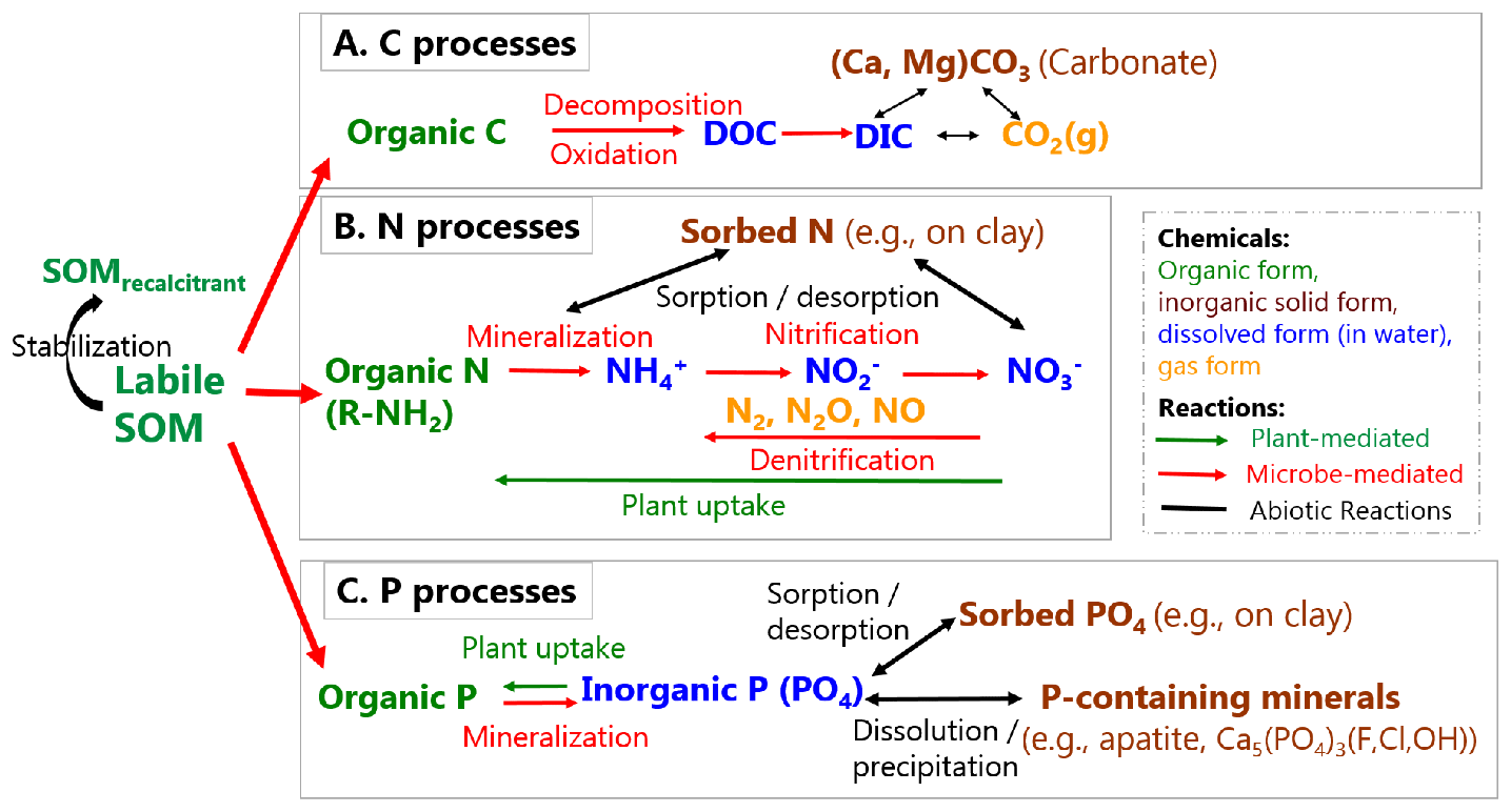
Figure 3Biotic and abiotic reactions relevant to the transformation of soil organic matter (SOM). SOM can become stabilized (recalcitrant) through sorption on clay and separation from reactants. Labile OM can decompose into inorganic forms, releasing C, N, and P that further transform into various forms (taken from Li, 2019, with permission from the Mineralogical Society of America).
Infiltration and vertical fluxes from the unsaturated to saturated layer in the shallow zone are based on the Richards equation, in which hydraulic water head H (i.e., the summation of water storage h and elevation head z) and hydraulic conductivity K determine the fluxes:
where di,inf and [m] are the thickness of infiltration layer and shallow-zone depth, respectively; Ki,inf [m s−1] is the hydraulic conductivity of the infiltration layer, the top 0.1 m of the subsurface that has different conductivity from the rest of subsurface; [m s−1] is the hydraulic conductivity in the vertical direction (i.e., weighted average of macropore Ki,macV and soil matrix Ki,satV, Eq. S7); Hi,sur [m] is the surface hydraulic water head (); and [m] are the shallow hydraulic water heads in the unsaturated and saturated layer, respectively. The lateral flow in the shallow saturated layer is calculated using Darcy's law:
where dij [m] is the distance between the centers of elements i and j; [m s−1] is the harmonic mean of shallow hydraulic conductivity in the horizontal direction between elements i () and j (). The interaction between the shallow saturated zone and stream channel also follows Eq. (5), except that the adjacent head is replaced by the level of stream water. Similar to the shallow zone, hydrological equations in the deep zone are detailed in the Supplement (Eqs. S1–S8).
3.2 Reactive transport equations
The governing advection dispersion reaction (ADR) equation for an arbitrary solute m in an element i is as follows (Bao et al., 2017):
where Vi [m3 total volume] is the total volume of element i; Sw,i [m3 water m−3 pore space] is soil water saturation; θi [m3 pore space m−3 total volume] is the porosity; Cm,i [mol m−3 water] is the aqueous concentration of species m; Nij is the number of fluxes from neighbor element j for element i, and Nij is 2 for the unsaturated zone (infiltration, recharge) with only vertical flows and 5 for saturated zone with flux from (or to) the unsaturated zone, from (or to) the deeper zone, and fluxes between i and three neighbor elements j in lateral flow directions for non-boundary grids; Aij [m2] is the grid area shared by i and its neighbor grid j; Dij [m2 s−1] is the hydrodynamic dispersion coefficient (i.e., sum of mechanical dispersion and effective diffusion coefficient) normal to the shared surface Aij; dij [m] is the distance between the center of i and its neighbor elements j; qij [m s−1] is the flow rate across Aij; Rm,i [mol s−1] is the total rate of kinetically controlled reactions in element i that involve species m; nm is the total number of independent primary species to be solved for reactive transport equations. Equation (6) states that the change in solute mass (the left term) is driven by dispersive transport, advective transport, and reactions (i.e., the first, second, and third right-hand side terms, respectively).
3.3 Biogeochemical processes and reaction kinetics
3.3.1 Biogeochemical processes
Here we discuss representative biogeochemical processes that involve plants and microbes that can be included in BioRT. BioRT differs from general water quality models that primarily target a few contaminants (e.g., N, P, metals). The framework of BioRT is flexible, and the users can define reactions and solutes of interest in the input files. For abiotic reactions such as mineral dissolution and surface complexation or ion exchange, readers are referred to Bao et al. (2017). Generally speaking, shallow soils contain more weathered materials and soil organic matters (SOMs) including roots, leaves, and microbes (Fig. 3). SOM can be decomposed partially into organic molecules that dissolve in water, i.e., dissolved organic carbon (DOC). It can also become oxidized completely into CO2, which can emit back to the atmosphere in gas form (Davidson, 2006) or transport and enter streams in the form of dissolved inorganic carbon (DIC). With coexisting cations (e.g., Ca, Mg), DIC can precipitate out and become carbonate minerals (e.g., CaCO3).
Organic matter (OM) decomposition releases organic nitrogen (R-NH2), which can further react to become and other nitrogen forms (N2, N2O, NO, , NO2) (Fig. 3). The gases can emit back to the atmosphere. Denitrification requires anoxic conditions and occurs less commonly in shallow soils owing to the pervasive presence of O2 (Sebestyen et al., 2019); denitrification can become important under wet conditions and in O2-depleted groundwater aquifers. Phosphorous (P) can be in organic forms in organic matter, sorbed on fine soil particles, dissolved in water, or in solid forms as P-containing minerals. Transformation of nutrients occurs through various bio-mediated or abiotic reactions. A representative P-containing mineral in the Earth's crust is apatite Ca5(PO4)3 (F, Cl, OH). Once liberated via rock dissolution, P is biologically assimilated and locked in organic forms. These organic forms have very low solubility, allowing them to bind on and be transported together with soil particles in the form of orthophosphate or pyro-diphosphate.
3.3.2 Reaction kinetics in natural soils
Rate dependence on temperature and soil moisture
Reactions such as soil respiration and plant uptake typically depend on environmental conditions (temperature or soil moisture). For example, in shallow oxic soils where organic carbon and O2 are often abundant, the rate law for carbon decomposition can be simplified to the following form assuming microorganism concentrations are relatively constant.
where the reaction rate r [mol s−1] depends on rate constant k [], the surface area A [m2] is a lumped parameter that quantitatively represents SOM content and biomass abundance, f(T) and f(Sw) describe the temperature and soil moisture dependence, respectively, f(Zw) can be included to account for the depth distribution of SOM (Seibert et al., 2009), and Zw [m] is the water table depth. An example for the depth distribution is (Weiler and McDonnell, 2006), with bm as the depth coefficient describing the gradient of SOM content over depth. Users can choose to include either one or all of these dependencies in input or database files.
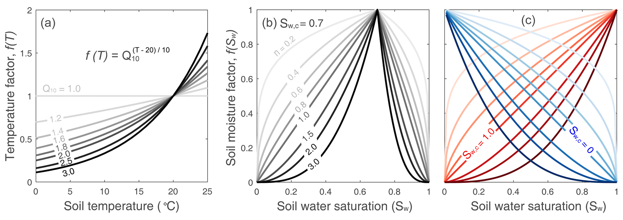
Figure 4Reaction rate dependence. (a) Function form of soil temperature dependence and (b, c) soil moisture dependence for reaction rates. The f(T) takes the Q10 form (Eq. 8). The soil moisture factor f(Sw) depends on Sw,c and n and soil water saturation Sw (Eq. 9). The soil moisture function can represent three types of behaviors: the threshold behavior (b, ), increase behavior (red in c, ), and decrease behavior (blue in c, ). Values of n=1 lead to a linear threshold dependence of Sw, while n<1 and n>1 lead to concave and convex dependences, respectively.
The temperature dependence follows a Q10-based form (Lloyd and Taylor, 1994; Davidson and Janssens, 2006) as follows:
where Q10 is the relative increase in reaction rates when temperature increases by 10 ∘C. Values of Q10 (Fig. 4a) can vary from 1.0 to 3.0, depending on climatic conditions, substrate availability, and ecosystem type (e.g., grassland, forest) (Davidson et al., 2006; Liu et al., 2017). The mean values are in the range of 1.4 to 2.5 (Zhou et al., 2009; Bracho et al., 2016). The Q10 value can be specified in the input file.
The soil moisture dependence function f(Sw) is coded in the following form:
Here Sw,c [0 to 1] is the critical soil moisture (saturation) at which rates are highest, and n is the exponent reflecting the dependence of rates on soil moisture. A typical n value is 2 (Yan et al., 2018) with a range between 1.2 and 3.0 (Hamamoto et al., 2010), depending on soil structure and texture. As shown in Fig. 4b, the form indicates an intermediate critical soil moisture Sw,c at which f(Sw) reaches its maximum. When , f(Sw) increases with Sw; when , f(Sw) decreases with Sw (Fig. 4b). Under the extreme conditions of Sw,c equaling 0 or 1, f(Sw) monotonically increases or decreases (Fig. 4c). The two parameters, Sw,c and n, determines the shape of the curve. They can be specified in input or database files. One can also choose not to have temperature or soil moisture dependence by choosing parameters that would lead to the value of the exponent being zero
Rate dependence on substrates: Monod kinetics and the biogeochemical redox ladder
Deeper groundwater aquifers often experience anoxic conditions that lead to processes such as denitrification or methanogenesis. This can also happen in wetlands or wet soils. Under such conditions, the rates of microbe-mediated redox reactions depend not only on temperature and soil moisture as discussed above, they also depend on concentrations of electron donors and non-oxygen electron acceptors (e.g., nitrate, iron oxides, sulfate) that are often limited under anoxic conditions (Bao et al., 2014; Li, 2019). The order of redox reactions typically follows the biogeochemical redox ladder, which is based on how much microbe can harvest energy by reducing different types of electron acceptors. Monod reaction rate laws are often used for quantifying rates of these redox conditions. These rate laws are detailed in Sect. S2 in the Supplement. Users can combine these Monod rate laws and the temperature and soil moisture dependence described above if needed.
3.4 Plant-related processes: root uptake of nitrate as an example
Nutrient uptake by plants is complex and remains poorly understood. A variety of plant uptake models exists with varying degrees of complexity (Neitsch et al., 2011; Fisher et al., 2010; Cai et al., 2016). These models are mostly based on a plant growth module or a supply and demand approach that often requires detailed phenological and plant attributes including growth cycle, root age and biomass, nutrient availability, and carbon allocation, in addition to local temperature and soil moisture (Dunbabin et al., 2002; Buysse et al., 1996; Fisher et al., 2010). Without a detailed mechanistic understanding, we assume a simple and operational approach. In Example 2, which we show later, for example, nitrate uptake was modeled with dependence on concentration, soil temperature and moisture, and rooting density (McMurtrie et al., 2012; Yan et al., 2012; Buljovcic and Engels, 2001).
where kuptake [L s−1] is the nitrate uptake rate, froot(dw) is the normalized rooting density term in the range of 0 to 1 as a function of water depth to the groundwater (dw). The rooting term (Eq. 14) was exponentially fitted (δ=0.013, λ=0.20) based on field measurements of root distribution along depth (Hasenmueller et al., 2017). It is common to observe a root density decrease exponentially in forests (López et al., 2001). Other forms of user-tailored plant uptake rate law can be added if needed.
The system of differential equations for water storage (e.g., Eqs. 1 and 2, and S1 and S2) is assembled into a global system of ordinary differential equations (ODEs). It is solved in CVODE (short for C-language Variable-coefficients ODE solver, https://computing.llnl.gov/projects/sundials/cvode, last access: 10 January 2021), a numerical ODE solver in the SUite of Nonlinear and Differential/ALgebraic equation Solvers (SUNDIALS) (Hindmarsh et al., 2005). In BioRT, the transport step is first solved with water by the preconditioned Krylov (iterative) method and the generalized minimal residual method (Saad and Schultz, 1986). All primary species in element i are then assembled in a local matrix and solved iteratively using the Crank–Nicolson and Newton–Raphson methods in CVODE (Bao et al., 2017).
Model verification
The BioRT module has been verified against CrunchTope under different transport and reaction conditions (Figs. S1–S7 in the Supplement). CrunchTope is a widely used subsurface reactive transport model (Steefel and Lasaga, 1994; Steefel et al., 2015) and is often used as a benchmark to verify other reactive transport models. Verification was performed under simplified hydrological conditions with 1-D column and constant flow rates such that it focuses on advection, diffusion, dispersion, and biogeochemical reactions. Specifically, three cases were verified. The phosphorus case that involves kinetics-controlled apatite dissolution and thermodynamics-controlled phosphorous speciation was first tested for solution accuracy of the bulk code that was inherited from the original RT-Flux-PIHM. Soil carbon and nitrogen processes were further verified for solution accuracy of the augmented BioRT module. Table S7 shows an average percent bias and Nash–Sutcliffe efficiency (NSE) of 1.1 % and 0.98, indicating a robust performance for a variety of solutes under different transport and reaction conditions. Note NSE ranges from −∞ to 1, with NSE=1 being the perfect fit (Moriasi et al., 2007).
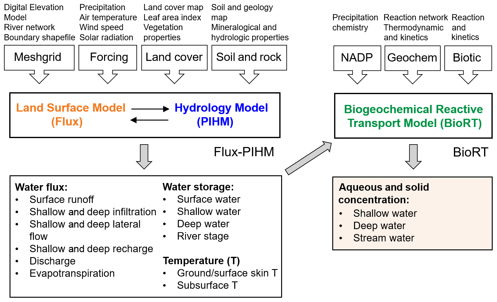
Figure 5Model structure, input, and output of BioRT-Flux-PIHM. The Flux-PIHM takes in watershed characteristics including topography (digital elevation model, DEM), land cover, shallow- and deep-zone properties, and meteorological forcing time series and solves for water storage and ground and soil temperature. BioRT takes in water- and temperature-related output from Flux-PIHM and additional inputs such as precipitation chemistry and shallow- and deep-water chemistry and biogeochemical kinetics parameters and solves for aqueous and solid concentrations in the shallow and deep zone and stream water. NADP stands for the National Atmospheric Deposition Program.
5.1 Model structure
The model takes meteorological forcing time series as input and solves for water storage and soil temperature, along with other hydrologic and land-surface states and fluxes (Fig. 5). BioRT reads in the model output of water and temperature from Flux-PIHM and solves biogeochemical reactive transport equations. At the timescale of months to years that are typical for BioRT simulations, alterations in solid phase properties, including porosity, permeability, and reactive surface area, are considered negligible such that hydrological parameters remain constant with time.
5.2 Data needs
The code sets up the model domain based on watershed characteristics including topography, land cover, and shallow- and deep-zone properties (Fig. 5). When the model is used in a spatially distributed form, the model domain is set up using elevation, land cover, soil, and geology maps supplied by the user. A useful data portal is the Geospatial Data Gateway (https://datagateway.nrcs.usda.gov, last access: 22 May 2019). Another geospatial data source is HydroTerre (http://www.hydroterre.psu.edu/, last access: 22 May 2019), where users can obtain data on elevation, land cover, geology, and soil (Leonard and Duffy, 2013). Meteorological forcing data can be downloaded from the North American Land Data Assimilation Systems Phase 2 (NLDAS-2, https://ldas.gsfc.nasa.gov/nldas/v2/forcing, , last access: 22 May 2019). The vegetation forcing, i.e., leaf area index (LAI), can be obtained from MODIS (Moderate Resolution Imaging Spectroradiometer, https://modis.gsfc.nasa.gov/data, last access: 22 May 2019). Other vegetation properties (e.g., shading fraction, rooting depth) can be adopted from, for example, the Noah vegetation parameter table embedded in the Weather Research and Forecasting model (WRF; Skamarock and Klemp, 2019). Local measurements from meteorological stations and field campaigns (e.g., land cover, soil, geology) can be used in the model. Initial water and solid phase chemistry can be based on measurements or general knowledge of the simulated sites. The form of reaction rate laws can be defined in the input files and calibrated to reproduce field data. Reaction thermodynamics, mostly equilibrium constants, are from the geochemical database EQ3/6 by default (Wolery, 1992). These reaction parameters can be modified when necessary. The model outputs include aqueous and solid concentrations of shallow and deep zones and stream water.
Table 1Example applications of BioRT-Flux-PIHM.
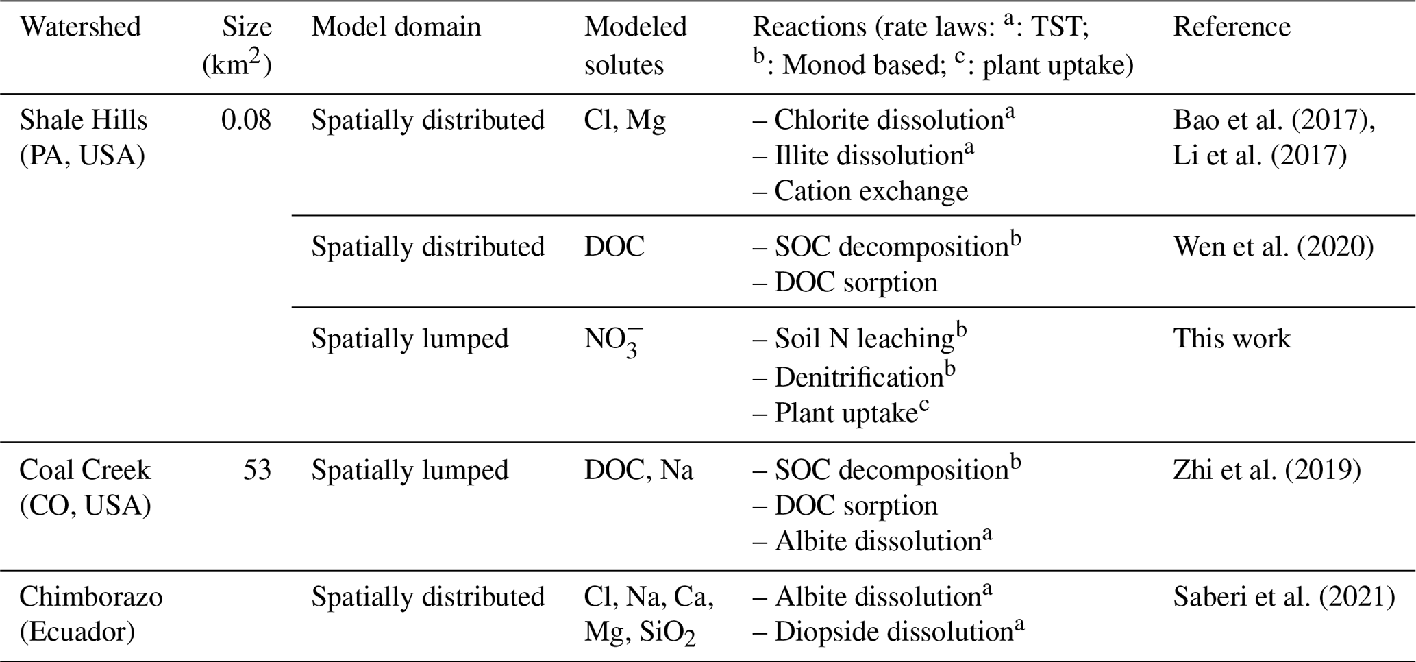
Note: transition state theory (TST) is a classic kinetic rate law for mineral dissolution and precipitation (Brantley et al., 2008) (Eq. S15); SOC stands for soil organic carbon.
5.2.1 Domain setup: spatially lumped and distributed domains
The domain can be set up at different spatial resolutions. A simple domain can be set up with two land grids representing two sides of a watershed connected by one river cell. This setup uses averaged properties without the need for spatial data. Alternatively, a complex domain can be set up to track “hot spots” of biogeochemical reactions using many grids with explicit representation of spatial details (e.g., topographic map, river network, land use map, soil and geology map, mineral distribution). The model domain can be set up using PIHMgis (http://www.pihm.psu.edu/pihmgis_home.html, last access: 22 May 2019), a standalone GIS interface for watershed delineation, domain decomposition, and parameter assignment (Bhatt et al., 2014). The same processes (e.g., hydrology, reaction network) can be setup in both types of spatial configurations. Auto-calibration is not built into the model, but a global calibration coefficient approach can be used to reduce parameter dimension and facilitate manual calibration. A typical model application requires 20 to 30 hydrological parameters to be calibrated. These parameters include land-surface parameters (e.g., canopy resistance, surface albedo), soil and geology parameters (e.g., hydraulic conductivity, porosity, Van Genuchten, macropore properties) (Shi et al., 2013). Reaction-related parameters (e.g., reaction rate constant, mineral surface area, Q10, Sw,c, and n) are additionally needed for calibration, the number of which depends on the numbers of reactions involved in a particular system.
The original RT-Flux-PIHM has been applied to understand processes related to the geogenic solutes of Cl and Mg at the Shale Hills watershed and for Na in a watershed on Chimborazo in the Ecuadorian Andes (Table 1). The new BioRT-Flux-PIHM has been demonstrated for understanding the dynamics of DOC and nitrate at Shale Hills and Coal Creek. This section will present one hydrology and two biogeochemical examples in the Susquehanna Shale Hills Critical Zone Observatory (SSHCZO), a small headwater watershed in central Pennsylvania, USA. The mean annual precipitation is approximately 1070 mm and the mean annual temperature is 10 ∘C (Brantley et al., 2018). Soil carbon storage and respiration and nitrogen budget and fluxes have been studied in detail (Andrews et al., 2011; Hasenmueller et al., 2015; Weitzman and Kaye, 2018). Modeling work has been conducted to understand hydrological dynamics (Shi et al., 2013; Xiao et al., 2019), transport of the non-reactive tracer Cl, and the weathering-derived solute Mg (Bao et al., 2017; Li et al., 2017a).
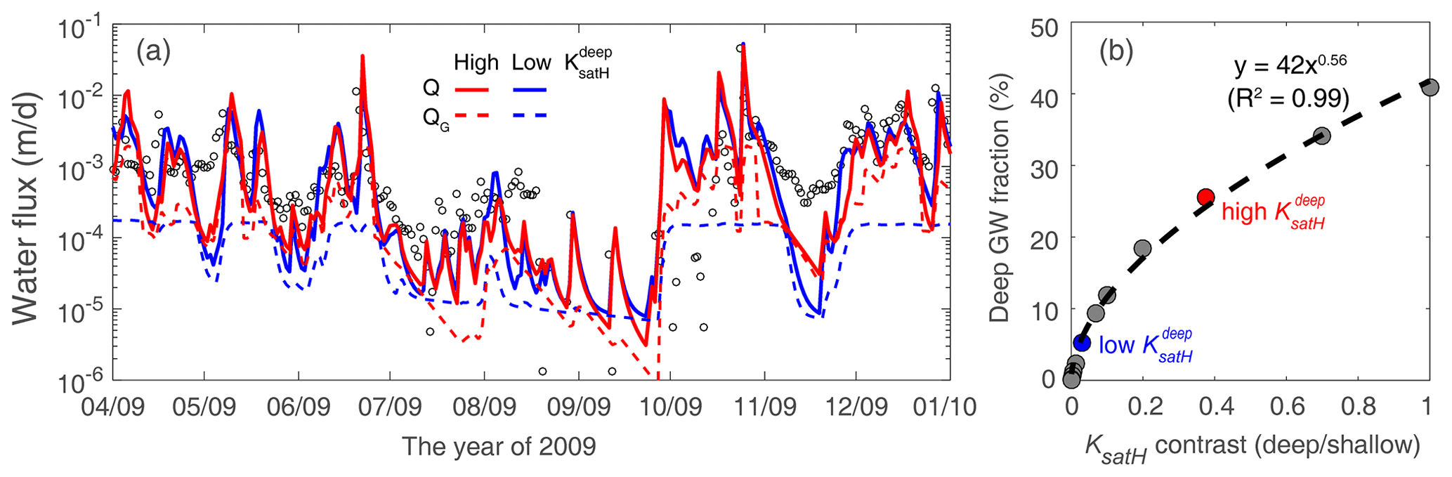
Figure 6(a) Hydraulic conductivity (KsatH) contrast controls the proportion of deep groundwater (QG). The cases of high ( m d−1, red) and low conductivity ( m d−1, blue) led to 26 % and 5.2 % of annual QG contribution to discharge (Q), respectively. (b) Deep-groundwater fraction as a function of KsatH contrast between the deep and shallow zone. The upper limit of the deep/shallow KsatH contrast was set to 1 as most watersheds have smaller KsatH in the deep zone than in the shallow zone. The two red and blue dots correspond to the two cases in (a).
6.1 Example 1: shallow and deep-water interactions
The model was set up using the spatially lumped mode with two grids and one river grid characterized by average land cover, soil, and rock properties based on previous work. The model assumed the dominant soil type (Weikert soil) at Shale Hills. The porosity of the deep zone was set to a tenth of the shallow soil porosity based on measurements of the groundwater aquifer (Brantley et al., 2018; Kuntz et al., 2011). In a headwater catchment like Shale Hills where the deep groundwater is most likely sourced from recharge, the deep-groundwater contribution to the stream can be primarily controlled by the hydraulic conductivity (KsatH) contrast between the deep and shallow zones (i.e., ). This is because the KsatH contrast determines the partitioning of infiltrating water between the shallow lateral flow and the downward recharge to the deep zone and then deep-groundwater flow. Two cases of high (red) and low (blue) were set up to showcase the control of KsatH contrast on deep groundwater (Fig. 6a). By changing the deep zone from 2.6 to 0.22 (m d−1), the annual deep-groundwater (QG) contribution to discharge (Q) decreased from 26 % to 5.2 %, although the total stream discharge remains the same. This indicates that the changing mostly changes the flow partitioning between the shallow soil flow and deeper groundwater flow into streams.
Several additional cases were further tested to examine the relationship between deep-groundwater fraction (%) of discharge and KsatH contrast. Figure 6b shows that the deep-groundwater fraction rapidly increases with the increasing ratio of , reaching a limit when the KsatH contrast is sufficiently high. The deep-groundwater contribution to the stream reaches ∼40 % when and are equal. In natural systems, we do see places, for example, karst formations, where groundwater contributes to more than 40 % (Hartmann et al., 2014; Husic, 2018). These places may have higher deeper conductivity than shallow soils due to the development of highly conductive conduits.
6.2 Example 2: nitrate dynamics in a spatially implicit domain
This example focuses on nitrate (), a dominant dissolved N form in water (Weitzman and Kaye, 2018). The N processes at Shale Hills include atmospheric N deposition, soil N leaching, stream export, denitrification, and plant uptake (Fig. 7). Based on field measurements, the atmospheric deposition at the site is the dominant N input; N export via discharge is only a small fraction (2.5 %) of atmospheric N input. Most deposited N is tightly cycled by plants or lost to the atmosphere via denitrification.
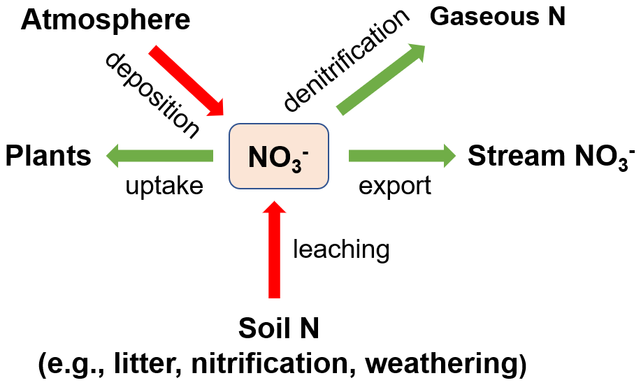
Figure 7Modeled nitrogen processes in Example 2. Atmospheric N deposition is the major N input; denitrification and plant uptake are the major N loss and sink. Export via discharge only occupies a small fraction.
The soil N leaching process was represented using a lumped reaction could represent the total rates of reactions including the decomposition of soil organic matter (SOM), nitrification, and rock weathering that generates . Its rate was assumed to depend on soil temperature and moisture and follows the equation rleach=kAf(T)f(Sw), where rleach [mol s−1] is the leaching rate, [] is the leaching rate constant (Regnier and Steefel, 1999), and A [m2] is the surface area that represents the contact area between substrates and N-transforming microbe. The surface area was calculated based on SOM volume fraction [m3 m−3], specific surface area (SSA, [m2 g−1]), substrate density [g cm−3], and element volume [m3].
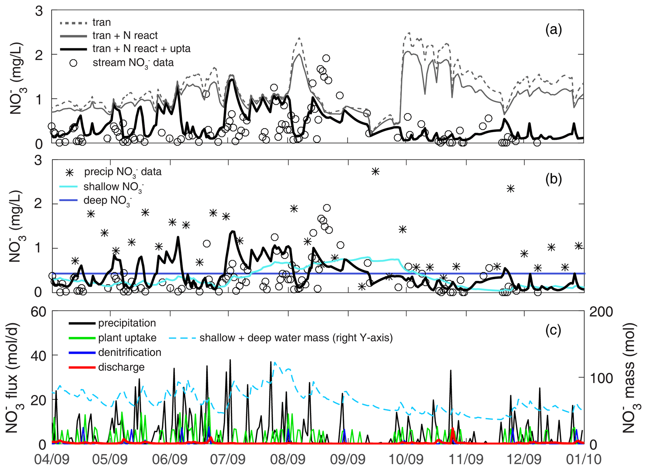
Figure 8Stream nitrate dynamics and fluxes at Shale Hills in Example 2. (a) Three simulation scenarios with different processes are demonstrated here: transport only (dashed line, tran), transport+N reaction (gray line, tran+N react), (thick black line, ), where N reactions include both nitrate leaching and denitrification (see Fig. 7); (b) nitrate concentration in precipitation and shallow and deep water; (c) nitrate fluxes and budget. Note that nitrate leaching was ignored in (b) due to its minimal flux as N deposition from rainfall was the dominant input (Weitzman and Kaye, 2018).
Denitrification converts to N2 gas under anaerobic conditions. Here this process was modeled by the Monod rate law with DOC as the electron donor, as the electron acceptor, and with an inhibition term f(O2) (Eq. S13). The reaction rate is
where [] is the denitrification rate constant (Regnier and Steefel, 1999) and half-saturation constants [µM] and [µM] (Regnier and Steefel, 1999). For soil N leaching and denitrification, the SSA were, respectively, tuned as and [m2 g−1] to reproduce observed stream nitrate dynamics. The calibrated values were orders of magnitude lower than the lab-measured SSA of natural materials (e.g., SOM, 0.6∼2 m2 g−1) (Rutherford et al., 1992). Such discrepancies between calibrated effective reactive surface area (i.e., solid–water contact area) and lab-measured absolute surface area are consistent with observations of field–lab discrepancies in the literature (Li et al., 2014; Heidari et al., 2017; Wen and Li, 2017, 2018). The uptake rate constant was calibrated by constraining the partitioning of N transformation flux between denitrification and plant uptake by the ratio of 1:5, a value estimated from field measurements of gaseous N outputs (3.53 ) and plant N uptake (18.3 ) (Weitzman and Kaye, 2018). The uptake rate constant in the deep zone (>2 m in depth) was considered negligible (Hasenmueller et al., 2017). Groundwater nitrate was initialized as 0.43 mg L−1, the average of measured groundwater concentration during 2009/10.
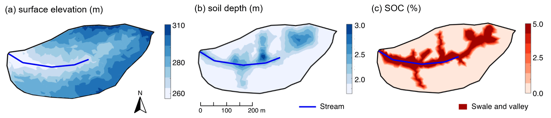
Figure 9Attributes of Shale Hills in the spatially distributed mode in Example 3: (a) surface elevation, (b) soil depth, and (c) soil organic carbon (SOC). The surface elevation was generated from lidar topographic data (criticalzone.org/shale-hills/data); soil depths and SOC were interpolated using ordinary kriging based on field surveys (Andrews et al., 2011; Lin, 2006). The SOC distribution in (c) was further simplified using the high, uniform SOC (5 % ) in swales and valley soils based on field survey (Andrews et al., 2011). Swales and valley floor areas were defined based on surface elevation via field survey and a 10 m resolution digital elevation model (Lin, 2006).
Temporal nitrate dynamics
Three cases were set up to understand and quantify the effects of different processes in determining nitrate dynamics (Fig. 8a). The transport-only case (dashed line, tran) simulates nitrate input from precipitation (at 1.4±0.96 mg L−1, based on the 2009 data of NADP PA42 site) and N transport but without any reactions. It overestimated stream nitrate data (0.33±0.39 mg L−1) throughout the year. The transport+N reactions case (gray line, tran+N react) has denitrification and soil N leaching processes but not plant uptake. These two reactions lowered the nitrate concentration slightly, as these two processes compensate each other in adding and removing nitrate from water. The case (thick black line, ) have all processes. It significantly lowered the nitrate concentration, especially in April–May and October–December. Nitrate peaks from May to July, exhibiting comparable levels of high nitrate concentration (Fig. 8b). It is noticeable that the three cases almost overlapped at these overestimated short nitrate peaks, suggesting nitrate-rich precipitation may not be routed into the subsurface where denitrification and plant uptake could occur.
Although precipitation from April to August accounted for 70 % of the total simulation period, larger storm events in October contributed more to nitrate export. Deeper groundwater had higher nitrate concentration than shallow water because most plant uptake occurred in the shallow zone. The nitrate fluxes into the deeper zone however only contributed 26 % of stream nitrate export at the annual scale, due to the relatively small groundwater contribution (9.5 %) to the stream. Denitrification and plant uptake largely occurred during wet spring with leaves growing. Denitrification peaks often appeared after major storm events because wet conditions facilitate denitrification. Comparing the three outfluxes (Fig. 8c), nitrate export via discharge (red) was negligible compared to denitrification (blue) and plant uptake (green). At the annual scale, stream export accounted for 9.5 %, whereas denitrification and plant uptake took up 15 % and 75 % of deposited , respectively. In other words, as Nitrate enters this system via precipitation, plant uptake can play a significant role in reducing nitrate level, indicating the precipitated nitrate is tightly cycled in the system.
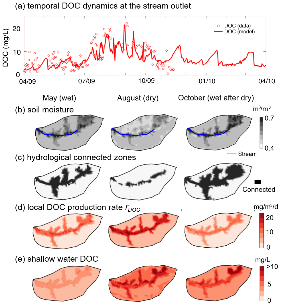
Figure 10(a) Temporal dynamics of stream DOC concentration; spatial profiles of (b) shallow soil moisture, (c) hydrologically connected zones, (d) local DOC production rates rDOC, and (e) shallow-water DOC concentration in May (wet), August (dry), and October (wet after dry) of 2009. The soil DOC and rDOC were high in swales and valley with relatively high shallow-water and SOC content. August had the highest shallow-water DOC concentration compared to May and October because most DOC accumulated in zones that are disconnected to the stream.
6.3 Example 3: DOC production and export in a spatially distributed domain
This example showcases the application of BioRT-Flux-PIHM in a spatially distributed mode. This work has been documented with full details in Wen et al. (2020). Here we only introduce some key features and capabilities in the spatially distributed mode. The Shale Hills catchment was discretized into 535 prismatic land elements and 20 stream segments through PIHMgis based on the topography (Fig. 9a). The heterogeneous distributions of soil depth and solid organic carbon within the domain (Fig. 9b and c) were interpolated through ordinary kriging based on field surveys (Andrews et al., 2011; Lin, 2006). Other soil and mineralogy properties such as hydraulic conductivity, van Genuchten parameters, and ion exchange capacity were spatially distributed following intensive field measurements (Jin and Brantley, 2011; Jin et al., 2010) (https://criticalzone.org/shale-hills/data/, last access: 22 May 2019).
6.3.1 Temporal and spatial patterns of DOC production and export
The model outputs followed the general trend of stream DOC measurements with the model evaluation index NSE of 0.55 for monthly DOC concentration (Fig. 10a). NSE values greater than 0.5 are considered good performance for the monthly water quality model (Moriasi et al., 2015). The model reproduced high DOC values (∼15 mg L−1) in the dry periods (July–September). The model enabled the identification of reaction hot spots. In May when soil water is relatively abundant, the valley and swales with deeper soils (Fig. 10b) are generally wetter compared to the hillslope and ridgetop, and are hydrologically connected to the stream (Fig. 10b and c). The distribution of local DOC production rate rDOC and DOC concentration followed that of SOC (Fig. 10c) and water content (Fig. 10b). Low rDOC in relatively dry planar hillslopes and uplands resulted in low soil water DOC. The average stream DOC (∼5 mg L−1) reflected soil water DOC in the valley and swales.
In August, the hydrologically connected zones with high water content shrank to the vicinity of the stream and riverbed. With high temperature in summer, rDOC increased 2-fold from May across the whole catchment while still exhibiting the highest values in the SOC-rich regions. Soil water DOC concentration increased by a factor of 2 because the produced DOC was trapped in low soil moisture areas that were not hydrologically connected to the stream. On the north side with low water content (Fig. 10b), the soil water DOC (∼7 mg L−1 on average) accumulated more than on the south side (∼5 mg L−1 on average). The high shallow-water DOC (∼10 mg L−1) in the stream vicinity dominated the stream DOC in August.
In October, precipitation wetted the catchment again. The hydrologically connected zones expanded beyond swales and the valley to the upland hillslopes (Fig. 10c). The increase in hydrological connectivity zones favored the mixing of shallow-water DOC sourced from upland hillslopes (low DOC), swales, and valley (high DOC) into streams rather than only from the stream vicinity with high DOC in the dry August, leading to a drop in stream DOC.
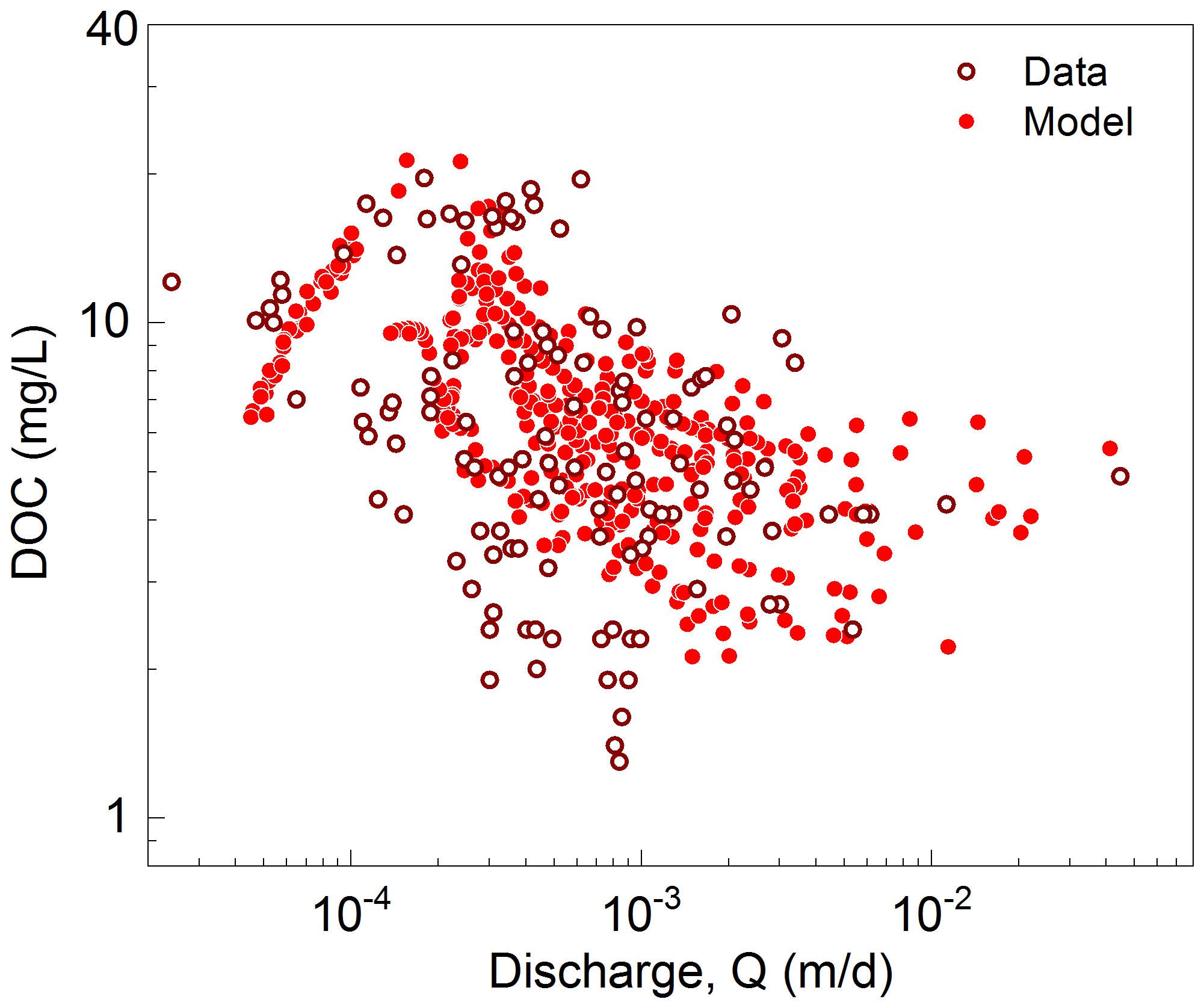
Figure 11Relationships between daily discharge (Q) and stream DOC concentration. With increasing Q, stream flow first shifted from the dominance of groundwater with low DOC at very low discharge to the predominance of organic-rich soil water from swales and valley at intermediate discharge. As the discharge increased further, the stream water switched to the dominance of high flow with lower DOC water from planar hillslopes and uplands, resulting in a dilution C–Q pattern at high discharge (from Wen et al., 2020, used with permission).
6.3.2 C–Q patterns
The DOC C–Q relationship showed a non-typical pattern with flushing first and transitioning into a dilution pattern, with an overall C–Q slope (Fig. 11). At low discharges ( m d−1) in the summer dry period, the stream DOC mainly came from the organic-rich swales and valley floor zones with high soil water DOC (Fig. 10e). With discharge increasing in wetter periods (i.e., spring and fall), the contribution from planar hillslopes and uplands with lower DOC concentration increased (Fig. 10e), leading to the dilution of stream DOC.
BioRT-Flux-PIHM brings the reactive transport modeling capabilities to the watershed scale, enabling the simulation of subsurface shallow and deep flow paths and biogeochemical reactions influenced by hydroclimatic conditions and land-surface interactions. The expanded model capability of simulating bio-mediated processes such as plant uptake, soil respiration, and microbe-mediated redox reactions enables the simulation of carbon and nutrient cycling in the shallow subsurface. The inclusion of the deep-groundwater zone allows the exploration of the effects of subsurface structure on hydrological partitioning between shallow soil lateral flow and deep groundwater and their relationships with stream discharge. Although not shown here, the model can also simulate deeper groundwater coming from regional aquifers across the outer boundary. This can be particularly useful for watersheds of higher stream orders, where a large proportion of deep water may come from nearby regional aquifers.
The advantage and disadvantages of simple vs. complex models have long been debated in the modeling community (Fatichi et al., 2016; Li et al., 2021; Wen et al., 2021). The computational cost of solving a spatially distributed, nonlinear, multi-component reactive transport model is high, posing challenges for the application of ensemble-based analysis. With additional reactions and transport processes, the model includes more functions (such as reaction kinetic rate laws) and parameters (e.g., reaction rate constants, surface area) than hydrological models. The complexity brings in issues of equifinality, uncertainty, and data demands (Beven, 2006; Kirchner et al., 1996). These issues will persist even though reactive transport models will be constrained by additional chemical data.
It is in this spirit of balancing the cost and gain that we present both spatially distributed and lumped modes for the BioRT model (Li et al., 2021). Compared to the distributed version, the spatially implicit model requires less spatial data and is computationally inexpensive. It can assess the average dynamics of water and solute dynamics and focus on the interacting processes without resolving spatial details. The lumped approach can accommodate basins with low data availability, and it can be easier for students to learn. In contrast, spatially explicit representations enable the exploration of the hot spots (e.g., swales and riparian zones with high soil water DOC concentrations in Fig. 10e) and their contribution to stream chemistry at different times. Spatial heterogeneities in watershed properties (e.g., soil types and depth, lithology, vegetation, biomass, and mineralogy) are ubiquitous in natural systems and are challenging to resolve. A general understanding of the linkage between local catchment features and catchment-scale dynamics (e.g., stream concentration dynamics and solute export pattern) is often lacking. The spatially distributed model provides a tool to explore these questions. Ultimately, the choice of the model complexity level depends on research questions that the model is set to answer and the available data. At the end, we all need to balance cost and gain when deciding to use a simple or complex model, striving to be “simple but not simplistic” (Beven and Lane, 2019).
This paper introduces the watershed-scale biogeochemical reactive transport code BioRT (short for BioRT-Flux-PIHM). The code integrates processes of land-surface interactions, surface hydrology, and multi-component biogeochemical reactive transport. The new development enables the simulation of (1) biotic reactions including plant uptake, soil respiration, and microbe-mediated redox reactions and (2) surface water interactions with groundwater from a deeper subsurface that still interacts with streams. BioRT has been verified against the widely used reactive transport code CrunchTope for soil carbon, nitrogen, and phosphorus processes. It has been applied to understand carbon, nitrogen, and weathering processes at Shale Hills in Pennsylvania, Coal Creek in Colorado, and the Chimborazo watershed in the Andes in Ecuador. Here we showcase the modeling capability of surface–groundwater interactions and reactive transport processes relevant to nitrate and DOC in Shale Hills in two simulation modes. One is in a spatially lumped mode using averaged properties and another is in a spatially distributed mode with a consideration of spatial heterogeneity. Results show that the deep-groundwater flow that interacts with the stream is primarily controlled by the hydraulic conductivity contrast between the shallow and the deep zones. Biogeochemical reactions in shallow soil primarily determine the stream water chemistry under high-flow conditions. The spatially lumped method with two lumped grids can capture the temporal dynamics of average behavior and mass balance; the spatially distributed running mode can be used to understand the spatial dynamics and to identify hot spots of reactions. The code can be used for biogeochemical reactive transport simulations in watersheds under diverse climate, land cover, and geology conditions.
The current model release (BioRT-Flux-PIHM v1.0) is archived at https://doi.org/10.5281/zenodo.3936073 (Zhi et al., 2020a). Documentation, source code, and examples are available in the GitHub repository: https://github.com/Li-Reactive-Water-Group/BioRT-Flux-PIHM (last access: 23 September 2021).
Field data (e.g., discharge, stream chemistry) are archived at Shale Hills data portal: https://criticalzone.org/dynamic_water/data (last access: 22 May 2019) (Shale Hills Data Portal, 2019) or maintained at HydroShare: https://www.hydroshare.org/group/147 (last access: 22 May 2019) (HydroShare, 2019).
The supplement related to this article is available online at: https://doi.org/10.5194/gmd-15-315-2022-supplement.
LL conceived the model idea and oversaw the model development. WZ coded the BioRT module, verified the code against the benchmark reactive transport model CrunchTope, and applied and tested the model at Shale Hills watershed. YS developed the deep-groundwater component and integrated the BioRT-Flux-PIHM v1.0 into the MM-PIHM family. WH, LS, KS, DK, BS, and GHCN tested the code during its development and contributed study cases.
The contact author has declared that neither they nor their co-authors have any competing interests.
Publisher's note: Copernicus Publications remains neutral with regard to jurisdictional claims in published maps and institutional affiliations.
We acknowledge the funding support from the Department of Energy, Subsurface Biogeochemistry Program and National Science Foundation. We appreciate data from the Susquehanna Shale Hills Critical Zone Observatory (SSHCZO) supported by National Science Foundation Grant EAR – 0725019 (Christopher J. Duffy), EAR – 1239285 (Susan L. Brantley), and EAR – 1331726 (Susan L. Brantley). Data were collected in Penn State's Stone Valley Forest, which is funded by the Penn State College of Agriculture Sciences, Department of Ecosystem Science and Management, and managed by the staff of the Forestlands Management Office.
This research has been supported by the Department of Energy, Subsurface Biogeochemistry Program (grant no. DE-SC0020146) and the National Science Foundation Hydrological Sciences (grant no. EAR-1758795).
This paper was edited by Min-Hui Lo and reviewed by three anonymous referees.
Adler, T., Underwood, K., Rizzo, D., Harpold, A., Sterle, G., Li, L., Wen, H., Stinson, L., Bristol, C., Lini, A., Perdrial, N., and Perdrial, J. N.: Drivers of Dissolved Organic Carbon Mobilization from Forested Headwater Catchments: A Multi Scaled Approach, Frontiers in Water, 3, 63, https://doi.org/10.3389/frwa.2021.578608, 2021.
Andrews, D. M., Lin, H., Zhu, Q., Jin, L., and Brantley, S. L.: Hot spots and hot moments of dissolved organic carbon export and soil organic carbon storage in the Shale Hills catchment, Vadose Zone J., 10, 943–954, 2011.
Bai, J., Zhang, G., Zhao, Q., Lu, Q., Jia, J., Cui, B., and Liu, X.: Depth-distribution patterns and control of soil organic carbon in coastal salt marshes with different plant covers, Sci. Rep.-UK, 6, 34835, https://doi.org/10.1038/srep34835, 2016.
Bailey, R., Rathjens, H., Bieger, K., Chaubey, I., and Arnold, J.: SWATMOD-Prep: Graphical User Interface for Preparing Coupled SWAT-MODFLOW Simulations, J. Am. Water Resour. As., 53, 400–410, https://doi.org/10.1111/1752-1688.12502, 2017.
Bao, C., Wu, H., Li, L., Newcomer, D., Long, P. E., and Williams, K. H.: Uranium Bioreduction Rates across Scales: Biogeochemical Hot Moments and Hot Spots during a Biostimulation Experiment at Rifle, Colorado, Environ. Sci. Technol., 48, 10116–10127, https://doi.org/10.1021/es501060d, 2014.
Bao, C., Li, L., Shi, Y., and Duffy, C.: Understanding watershed hydrogeochemistry: 1. Development of RT-Flux-PIHM, Water Resour. Res., 53, 2328–2345, 2017.
Basu, N. B., Destouni, G., Jawitz, J. W., Thompson, S. E., Loukinova, N. V., Darracq, A., Zanardo, S., Yaeger, M., Sivapalan, M., Rinaldo, A., and Rao, P. S. C.: Nutrient loads exported from managed catchments reveal emergent biogeochemical stationarity, Geophys. Res. Lett., 37, L23404, https://doi.org/10.1029/2010GL045168, 2010.
Benettin, P., Fovet, O., and Li, L.: Nitrate removal and young stream water fractions at the catchment scale, Hydrol. Process., 34, 2725–2738, https://doi.org/10.1002/hyp.13781, 2020.
Beven, K.: How far can we go in distributed hydrological modelling?, Hydrol. Earth Syst. Sci., 5, 1–12, https://doi.org/10.5194/hess-5-1-2001, 2001.
Beven, K.: A manifesto for the equifinality thesis, J. Hydrol., 320, 18–36, https://doi.org/10.1016/j.jhydrol.2005.07.007, 2006.
Beven, K. and Lane, S.: Invalidation of Models and Fitness-for-Purpose: A Rejectionist Approach, in: Computer Simulation Validation: Fundamental Concepts, Methodological Frameworks, and Philosophical Perspectives, edited by: Beisbart, C. and Saam, N. J., Springer International Publishing, Cham, 145–171, 2019.
Bhatt, G., Kumar, M., and Duffy, C. J.: A tightly coupled GIS and distributed hydrologic modeling framework, Environ. Modell. Softw., 62, 70–84, https://doi.org/10.1016/j.envsoft.2014.08.003, 2014.
Botter, M., Li, L., Hartmann, J., Burlando, P., and Fatichi, S.: Depth of Solute Generation Is a Dominant Control on Concentration-Discharge Relations, Water Resour. Res., 56, e2019WR026695, https://doi.org/10.1029/2019WR026695, 2020.
Bracho, R., Natali, S., Pegoraro, E., Crummer, K. G., Schädel, C., Celis, G., Hale, L., Wu, L., Yin, H., and Tiedje, J. M.: Temperature sensitivity of organic matter decomposition of permafrost-region soils during laboratory incubations, Soil Biol. Biochem., 97, 1–14, 2016.
Brantley, S. L., Kubicki, J. D., and White, A. F.: Kinetics of water–rock interaction, Springer, New York, 2008.
Brantley, S. L., White, T., West, N., Williams, J. Z., Forsythe, B., Shapich, D., Kaye, J., Lin, H., Shi, Y. N., Kaye, M., Herndon, E., Davis, K. J., He, Y., Eissenstat, D., Weitzman, J., DiBiase, R., Li, L., Reed, W., Brubaker, K., and Gu, X.: Susquehanna Shale Hills Critical Zone Observatory: Shale Hills in the Context of Shaver's Creek Watershed, Vadose Zone J., 17, 1–19, ARTN 180092, https://doi.org/10.2136/vzj2018.04.0092, 2018.
Buljovcic, Z. and Engels, C.: Nitrate uptake ability by maize roots during and after drought stress, Plant Soil, 229, 125–135, 2001.
Buysse, J., Smolders, E., and Merckx, R.: Modelling the uptake of nitrate by a growing plant with an adjustable root nitrate uptake capacity, Plant Soil, 181, 19–23, 1996.
Cai, X., Yang, Z.-L., Fisher, J. B., Zhang, X., Barlage, M., and Chen, F.: Integration of nitrogen dynamics into the Noah-MP land surface model v1.1 for climate and environmental predictions, Geosci. Model Dev., 9, 1–15, https://doi.org/10.5194/gmd-9-1-2016, 2016.
Davidson, E. A. and Janssens, I. A.: Temperature sensitivity of soil carbon decomposition and feedbacks to climate change, Nature, 440, 165–173, https://doi.org/10.1038/nature04514, 2006.
Davidson, E. A., Janssens, I. A., and Luo, Y.: On the variability of respiration in terrestrial ecosystems: moving beyond Q10, Glob. Change Biol., 12, 154–164, 2006.
Dingman, S. L.: Physical hydrology, Waveland press, Long Grove, 2015.
Dunbabin, V. M., Diggle, A. J., Rengel, Z., and Van Hugten, R.: Modelling the interactions between water and nutrient uptake and root growth, Plant Soil, 239, 19–38, 2002.
Fatichi, S., Vivoni, E. R., Ogden, F. L., Ivanov, V. Y., Mirus, B., Gochis, D., Downer, C. W., Camporese, M., Davison, J. H., and Ebel, B.: An overview of current applications, challenges, and future trends in distributed process-based models in hydrology, J. Hydrol., 537, 45–60, 2016.
Fatichi, S., Manzoni, S., Or, D., and Paschalis, A.: A Mechanistic Model of Microbially Mediated Soil Biogeochemical Processes: A Reality Check, Global Biogeochem. Cy., 33, 620–648, https://doi.org/10.1029/2018gb006077, 2019.
Fisher, J., Sitch, S., Malhi, Y., Fisher, R., Huntingford, C., and Tan, S. Y.: Carbon cost of plant nitrogen acquisition: A mechanistic, globally applicable model of plant nitrogen uptake, retranslocation, and fixation, Global Biogeochem. Cy., 24, GB1014, https://doi.org/10.1029/2009GB003621, 2010.
Gatel, L., Lauvernet, C., Carluer, N., Weill, S., Tournebize, J., and Paniconi, C.: Global evaluation and sensitivity analysis of a physically based flow and reactive transport model on a laboratory experiment, Environ. Modell. Softw., 113, 73–83, https://doi.org/10.1016/j.envsoft.2018.12.006, 2019.
Godsey, S. E., Kirchner, J. W., and Clow, D. W.: Concentration–discharge relationships reflect chemostatic characteristics of US catchments, Hydrol. Process., 23, 1844–1864, https://doi.org/10.1002/hyp.7315, 2009.
Godsey, S. E., Hartmann, J., and Kirchner, J. W.: Catchment chemostasis revisited: Water quality responds differently to variations in weather and climate, Hydrol. Process., 33, 3056–3069, https://doi.org/10.1002/hyp.13554, 2019.
Grathwohl, P., Rügner, H., Wöhling, T., Osenbrück, K., Schwientek, M., Gayler, S., Wollschläger, U., Selle, B., Pause, M., and Delfs, J.-O.: Catchments as reactors: a comprehensive approach for water fluxes and solute turnover, Environ. Earth Sci., 69, 317–333, 2013.
Green, T. R.: Linking climate change and groundwater, in: Integrated groundwater management, Springer, Cham, 97–141, 2016.
Guevara Ochoa, C., Medina Sierra, A., Vives, L., Zimmermann, E., and Bailey, R.: Spatio‐temporal patterns of the interaction between groundwater and surface water in plains, Hydrol. Process., 34, 1371–1392, 2020.
Gurdak, J. J.: Groundwater: Climate-induced pumping, Nat. Geosci., 10, 71, 2017.
Hamamoto, S., Moldrup, P., Kawamoto, K., and Komatsu, T.: Excluded-volume expansion of Archie's law for gas and solute diffusivities and electrical and thermal conductivities in variably saturated porous media, Water Resour. Res., 46, W06514, https://doi.org/10.1029/2009WR008424, 2010.
Hartley, I. P., Heinemeyer, A., and Ineson, P.: Effects of three years of soil warming and shading on the rate of soil respiration: substrate availability and not thermal acclimation mediates observed response, Glob. Change Biol., 13, 1761–1770, https://doi.org/10.1111/j.1365-2486.2007.01373.x, 2007.
Hartmann, J., Lauerwald, R., and Moosdorf, N.: A brief overview of the GLObal RIver CHemistry Database, GLORICH, Proced. Earth Plan. Sc., 10, 23–27, 2014.
Hasenmueller, E. A., Jin, L., Stinchcomb, G. E., Lin, H., Brantley, S. L., and Kaye, J. P.: Topographic controls on the depth distribution of soil CO2 in a small temperate watershed, Appl. Geochem., 63, 58–69, 2015.
Hasenmueller, E. A., Gu, X., Weitzman, J. N., Adams, T. S., Stinchcomb, G. E., Eissenstat, D. M., Drohan, P. J., Brantley, S. L., and Kaye, J. P.: Weathering of rock to regolith: The activity of deep roots in bedrock fractures, Geoderma, 300, 11–31, 2017.
Heidari, P., Li, L., Jin, L., Williams, J. Z., and Brantley, S. L.: A reactive transport model for Marcellus shale weathering, Geochim. Cosmochim. Ac., 217, 421–440, 2017.
Herndon, E. M., Dere, A. L., Sullivan, P. L., Norris, D., Reynolds, B., and Brantley, S. L.: Landscape heterogeneity drives contrasting concentration–discharge relationships in shale headwater catchments, Hydrol. Earth Syst. Sci., 19, 3333–3347, https://doi.org/10.5194/hess-19-3333-2015, 2015.
Hindmarsh, A. C., Brown, P. N., Grant, K. E., Lee, S. L., Serban, R., Shumaker, D. E., and Woodward, C. S.: SUNDIALS: Suite of nonlinear and differential/algebraic equation solvers, ACM T. Math. Software, 31, 363–396, 2005.
Hubbard, S. S., Williams, K. H., Agarwal, D., Banfield, J., Beller, H., Bouskill, N., Brodie, E., Carroll, R., Dafflon, B., and Dwivedi, D.: The East River, Colorado, Watershed: A mountainous community testbed for improving predictive understanding of multiscale hydrological-biogeochemical dynamics, Vadose Zone J., 17, 1–25, https://doi.org/10.2136/vzj2018.03.0061, 2018.
Husic, A.: Numerical modeling and isotope tracers to investigate karst biogeochemistry and transport processes, Doctoral Dissertation, https://doi.org/10.13023/etd.2018.322, 2018.
HydroShare: CZO Shale Hills, HydroShare [data set], available at: https://www.hydroshare.org/group/147, last access: 22 May 2019.
Jin, L. and Brantley, S. L.: Soil chemistry and shale weathering on a hillslope influenced by convergent hydrologic flow regime at the Susquehanna/Shale Hills Critical Zone Observatory, Appl. Geochem., 26, S51–S56, https://doi.org/10.1016/j.apgeochem.2011.03.027, 2011.
Jin, L. X., Ravella, R., Ketchum, B., Bierman, P. R., Heaney, P., White, T., and Brantley, S. L.: Mineral weathering and elemental transport during hillslope evolution at the Susquehanna/Shale Hills Critical Zone Observatory, Geochim. Cosmochim. Ac., 74, 3669–3691, https://doi.org/10.1016/j.gca.2010.03.036, 2010.
Keune, J., Gasper, F., Goergen, K., Hense, A., Shrestha, P., Sulis, M., and Kollet, S.: Studying the influence of groundwater representations on land surface-atmosphere feedbacks during the European heat wave in 2003, J. Geophys. Res.-Atmos., 121, 13301–13325, https://doi.org/10.1002/2016JD025426, 2016.
Kirchner, J. W., Hooper, R. P., Kendall, C., Neal, C., and Leavesley, G.: Testing and validating environmental models, Sci. Total Environ., 183, 33–47, https://doi.org/10.1016/0048-9697(95)04971-1, 1996.
Kuntz, B. W., Rubin, S., Berkowitz, B., and Singha, K.: Quantifying Solute Transport at the Shale Hills Critical Zone Observatory, Vadose Zone J., 10, 843–857, https://doi.org/10.2136/vzj2010.0130, 2011.
Leonard, L. and Duffy, C. J.: Essential terrestrial variable data workflows for distributed water resources modeling, Environ. Modell. Softw., 50, 85–96, 2013.
Li, L.: Watershed reactive transport, Reviews in Mineralogy and Geochemistry, 85, 381–418, 2019.
Li, L., Salehikhoo, F., Brantley, S. L., and Heidari, P.: Spatial zonation limits magnesite dissolution in porous media, Geochim. Cosmochim. Ac., 126, 555–573, https://doi.org/10.1016/j.gca.2013.10.051, 2014.
Li, L., Bao, C., Sullivan, P. L., Brantley, S., Shi, Y., and Duffy, C.: Understanding watershed hydrogeochemistry: 2. Synchronized hydrological and geochemical processes drive stream chemostatic behavior, Water Resour. Res., 53, 2346–2367, 2017a.
Li, L., Maher, K., Navarre-Sitchler, A., Druhan, J., Meile, C., Lawrence, C., Moore, J., Perdrial, J., Sullivan, P., Thompson, A., Jin, L., Bolton, E. W., Brantley, S. L., Dietrich, W. E., Mayer, K. U., Steefel, C. I., Valocchi, A., Zachara, J., Kocar, B., McIntosh, J., Tutolo, B. M., Kumar, M., Sonnenthal, E., Bao, C., and Beisman, J.: Expanding the role of reactive transport models in critical zone processes, Earth-Sci. Rev., 165, 280–301, https://doi.org/10.1016/j.earscirev.2016.09.001, 2017b.
Li, L., Sullivan, P. L., Benettin, P., Cirpka, O. A., Bishop, K., Brantley, S. L., Knapp, J. L. A., Meerveld, I., Rinaldo, A., Seibert, J., Wen, H., and Kirchner, J. W.: Toward catchment hydro-biogeochemical theories, WIREs Water, https://doi.org/10.1002/wat2.1495, 2021.
Lin, H.: Temporal stability of soil moisture spatial pattern and subsurface preferential flow pathways in the Shale Hills Catchment, Vadose Zone J., 5, 317–340, 2006.
Lindström, G., Rosberg, J., and Arheimer, B.: Parameter Precision in the HBV-NP Model and Impacts on Nitrogen Scenario Simulations in the Rönneå River, Southern Sweden, AMBIO, 34, 533–537, 2005.
Lindström, G., Pers, C., Rosberg, J., Strömqvist, J., and Arheimer, B.: Development and testing of the HYPE (Hydrological Predictions for the Environment) water quality model for different spatial scales, Hydrol. Res., 41, 295–319, https://doi.org/10.2166/nh.2010.007, 2010.
Liu, Y., Wang, C., He, N., Wen, X., Gao, Y., Li, S., Niu, S., Butterbach-Bahl, K., Luo, Y., and Yu, G.: A global synthesis of the rate and temperature sensitivity of soil nitrogen mineralization: latitudinal patterns and mechanisms, Glob. Change Biol., 23, 455–464, 2017.
Lloyd, J. and Taylor, J. A.: On the Temperature Dependence of Soil Respiration, Funct. Ecol., 8, 315–323, https://doi.org/10.2307/2389824, 1994.
López, B., Sabaté, S., and Gracia, C.: Vertical distribution of fine root density, length density, area index and mean diameter in a Quercus ilex forest, Tree Physiol., 21, 555–560, 2001.
McMurtrie, R. E., Iversen, C. M., Dewar, R. C., Medlyn, B. E., Näsholm, T., Pepper, D. A., and Norby, R. J.: Plant root distributions and nitrogen uptake predicted by a hypothesis of optimal root foraging, Ecol. Evol., 2, 1235–1250, 2012.
Miller, M. P., Tesoriero, A. J., Hood, K., Terziotti, S., and Wolock, D. M.: Estimating Discharge and Nonpoint Source Nitrate Loading to Streams From Three End-Member Pathways Using High-Frequency Water Quality Data, Water Resour. Res., 53, 10201–10216, https://doi.org/10.1002/2017wr021654, 2017.
Moatar, F., Abbott, B. W., Minaudo, C., Curie, F., and Pinay, G.: Elemental properties, hydrology, and biology interact to shape concentration-discharge curves for carbon, nutrients, sediment, and major ions, Water Resour. Res., 53, 1270–1287, 2017.
Moriasi, D. N., Arnold, J. G., Van Liew, M. W., Bingner, R. L., Harmel, R. D., and Veith, T. L.: Model evaluation guidelines for systematic quantification of accuracy in watershed simulations, T. Asabe, 50, 885–900, 2007.
Moriasi, D. N., Gitau, M. W., Pai, N., and Daggupati, P.: Hydrologic and water quality models: Performance measures and evaluation criteria, T. Asabe, 58, 1763–1785, 2015.
Musolff, A., Schmidt, C., Selle, B., and Fleckenstein, J. H.: Catchment controls on solute export, Adv. Water Resour., 86, 133–146, https://doi.org/10.1016/j.advwatres.2015.09.026, 2015.
Neitsch, S. L., Arnold, J. G., Kiniry, J. R., and Williams, J. R.: Soil and water assessment tool theoretical documentation version 2009, Texas Water Resources Institute, College Station, 2011.
Qu, Y. and Duffy, C. J.: A semidiscrete finite volume formulation for multiprocess watershed simulation, Water Resour. Res., 43, W08419, https://doi.org/10.1029/2006WR005752, 2007.
Regnier, P. and Steefel, C. I.: A high resolution estimate of the inorganic nitrogen flux from the Scheldt estuary to the coastal North Sea during a nitrogen-limited algal bloom, spring 1995, Geochim. Cosmochim. Ac., 63, 1359–1374, https://doi.org/10.1016/s0016-7037(99)00034-4, 1999.
Rutherford, D. W., Chiou, C. T., and Kile, D. E.: Influence of soil organic matter composition on the partition of organic compounds, Environ. Sci. Technol., 26, 336–340, 1992.
Saad, Y. and Schultz, M. H.: GMRES: A generalized minimal residual algorithm for solving nonsymmetric linear systems, SIAM J. Sci. Stat. Comp., 7, 856–869, 1986.
Saberi, L., Crystal Ng, G. H., Nelson, L., Zhi, W., Li, L., La Frenierre, J., and Johnstone, M.: Spatiotemporal Drivers of Hydrochemical Variability in a Tropical Glacierized Watershed in the Andes, Water Resour. Res., 57, e2020WR028722, https://doi.org/10.1029/2020WR028722, 2021.
Scudeler, C., Pangle, L., Pasetto, D., Niu, G.-Y., Volkmann, T., Paniconi, C., Putti, M., and Troch, P.: Multiresponse modeling of variably saturated flow and isotope tracer transport for a hillslope experiment at the Landscape Evolution Observatory, Hydrol. Earth Syst. Sci., 20, 4061–4078, https://doi.org/10.5194/hess-20-4061-2016, 2016.
Sebestyen, S. D., Ross, D. S., Shanley, J. B., Elliott, E. M., Kendall, C., Campbell, J. L., Dail, D. B., Fernandez, I. J., Goodale, C. L., and Lawrence, G. B.: Unprocessed Atmospheric Nitrate in Waters of the Northern Forest Region in the US and Canada, Environ. Sci. Technol., 53, 3620–3633, 2019.
Seibert, J., Grabs, T., Köhler, S., Laudon, H., Winterdahl, M., and Bishop, K.: Linking soil- and stream-water chemistry based on a Riparian Flow-Concentration Integration Model, Hydrol. Earth Syst. Sci., 13, 2287–2297, https://doi.org/10.5194/hess-13-2287-2009, 2009.
Shale Hills Data Portal: Water Data, Shale Hills Data Portal [data set], available at: https://criticalzone.org/dynamic_water/data, last access: 22 May 2019.
Shi, Y.: Development of a land surface hydrologic modeling and data assimilation system for the study of subsurface-land surface interaction, Doctoral Dissertation, Penn State University, State College, available at: https://etda.libraries.psu.edu/files/final_submissions/7621 (last access: 22 May 2019), 2012.
Shi, Y., Davis, K. J., Duffy, C. J., and Yu, X.: Development of a coupled land surface hydrologic model and evaluation at a critical zone observatory, J. Hydrometeorol., 14, 1401–1420, 2013.
Skamarock, W. and Klemp, J.: A Description of the Advanced Research WRF Model Version 4. Ncar Technical Notes, No, NCAR/TN-556+STR, Boulder, 2019.
Steefel, C., Appelo, C., Arora, B., Jacques, D., Kalbacher, T., Kolditz, O., Lagneau, V., Lichtner, P., Mayer, K. U., and Meeussen, J.: Reactive transport codes for subsurface environmental simulation, Comput. Geosci., 19, 445–478, 2015.
Steefel, C. I. and Lasaga, A. C.: A coupled model for transport of multiple chemical species and kinetic precipitation/dissolution reactions with application to reactive flow in single phase hydrothermal systems, Am. J. Sci., 294, 529–592, 1994.
Stewart, B., Shanley, J. B., Kirchner, J. W., Norris, D., Adler, T., Bristol, C., Harpold AA, Perdrial, J. N., Rizzo, D. M., Sterle, G., Underwood, K. L., Wen, H., and Li, L.: Streams as mirrors: reading subsurface water chemistry from stream chemistry, Water Resour. Res., 57, e2021WR029931, https://doi.org/10.1029/2021WR029931, 2021.
Sullivan, P. L., Hynek, S. A., Gu, X., Singha, K., White, T., West, N., Kim, H., Clarke, B., Kirby, E., Duffy, C., and Brantley, S. L.: Oxidative dissolution under the channel leads geomorphological evolution at the Shale Hills catchment, Am. J. Sci., 316, 981–1026, https://doi.org/10.2475/10.2016.02, 2016.
Taylor, R. G., Scanlon, B., Döll, P., Rodell, M., Van Beek, R., Wada, Y., Longuevergne, L., Leblanc, M., Famiglietti, J. S., and Edmunds, M.: Ground water and climate change, Nat. Clim. Change, 3, 322, 2013.
van der Velde, Y., de Rooij, G. H., Rozemeijer, J. C., van Geer, F. C., and Broers, H. P.: Nitrate response of a lowland catchment: On the relation between stream concentration and travel time distribution dynamics, Water Resour. Res., 46, W11534, https://doi.org/10.1029/2010WR009105, 2010.
Weiler, M. and McDonnell, J. R. J.: Testing nutrient flushing hypotheses at the hillslope scale: A virtual experiment approach, J. Hydrol., 319, 339–356, https://doi.org/10.1016/j.jhydrol.2005.06.040, 2006.
Weitzman, J. N. and Kaye, J. P.: Nitrogen Budget and Topographic Controls on Nitrous Oxide in a Shale-Based Watershed, J. Geophys. Res.-Biogeo., 123, 1888–1908, 2018.
Wen, H. and Li, L.: An upscaled rate law for magnesite dissolution in heterogeneous porous media, Geochim. Cosmochim. Ac., 210, 289–305, 2017.
Wen, H. and Li, L.: An upscaled rate law for mineral dissolution in heterogeneous media: The role of time and length scales, Geochim. Cosmochim. Ac., 235, 1–20, 2018.
Wen, H., Perdrial, J., Abbott, B. W., Bernal, S., Dupas, R., Godsey, S. E., Harpold, A., Rizzo, D., Underwood, K., Adler, T., Sterle, G., and Li, L.: Temperature controls production but hydrology regulates export of dissolved organic carbon at the catchment scale, Hydrol. Earth Syst. Sci., 24, 945–966, https://doi.org/10.5194/hess-24-945-2020, 2020.
Wen, H., Brantley, S. L., Davis, K. J., Duncan, J. M., and Li, L.: The Limits of Homogenization: What Hydrological Dynamics can a Simple Model Represent at the Catchment Scale?, Water Resour. Res., 57, e2020WR029528, https://doi.org/10.1029/2020WR029528, 2021.
Wolery, T. J.: EQ3/6, a software package for geochemical modeling of aqueous systems: package overview and installation guide (version 7.0), Lawrence Livermore National Lab, 1992.
Xiao, D., Shi, Y., Brantley, S. L., Forsythe, B., DiBiase, R., Davis, K., and Li, L.: Streamflow Generation From Catchments of Contrasting Lithologies: The Role of Soil Properties, Topography, and Catchment Size, Water Resour. Res., 55, 9234–9257, https://doi.org/10.1029/2018WR023736, 2019.
Xiao, D., Brantley, S. L., and Li, L.: Vertical Connectivity Regulates Water Transit Time and Chemical Weathering at the Hillslope Scale, Water Resour. Res., 57, e2020WR029207, https://doi.org/10.1029/2020WR029207, 2021.
Yan, Q., Duan, Z., Mao, J., Li, X., and Dong, F.: Effects of root-zone temperature and N, P, and K supplies on nutrient uptake of cucumber (Cucumis sativus L.) seedlings in hydroponics, Soil Sci. Plant Nutr., 58, 707–717, 2012.
Yan, Z., Bond-Lamberty, B., Todd-Brown, K. E., Bailey, V. L., Li, S., Liu, C., and Liu, C.: A moisture function of soil heterotrophic respiration that incorporates microscale processes, Nat. Commun., 9, 2562, https://doi.org/10.1038/s41467-018-04971-6, 2018.
Zarnetske, J. P., Bouda, M., Abbott, B. W., Saiers, J., and Raymond, P. A.: Generality of hydrologic transport limitation of watershed organic carbon flux across ecoregions of the United States, Geophys. Res. Lett., 45, 11702–11711, 2018.
Zhi, W. and Li, L.: The Shallow and Deep Hypothesis: Subsurface Vertical Chemical Contrasts Shape Nitrate Export Patterns from Different Land Uses, Environ. Sci. Technol., 54, 11915–11928, https://doi.org/10.1021/acs.est.0c01340, 2020.
Zhi, W., Li, L., Dong, W., Brown, W., Kaye, J., Steefel, C., and Williams, K. H.: Distinct Source Water Chemistry Shapes Contrasting Concentration-Discharge Patterns, Water Resour. Res., 55, 4233–4251, https://doi.org/10.1029/2018wr024257, 2019.
Zhi, W., Shi, Y., Wen, H., Saberi, L., Ng, G.-H. C., Sadayappan, K., Kerins, D., Stewart, B., and Li, L.: BioRT-Flux-PIHM-v1.0, v1.0, Zenodo [code], https://doi.org/10.5281/zenodo.3936073, 2020a.
Zhi, W., Williams, K. H., Carroll, R. W. H., Brown, W., Dong, W., Devon Kerins, D., and Li, L.: Significant stream chemistry response to temperature variations in a high-elevation mountain watershed, Communications Earth & Environment, 1, 43, https://doi.org/10.1038/s43247-020-00039-w, 2020b.
Zhou, T., Shi, P., Hui, D., and Luo, Y.: Global pattern of temperature sensitivity of soil heterotrophic respiration (Q10) and its implications for carbon-climate feedback, J. Geophys. Res., 114, G02016, https://doi.org/10.1029/2008JG000850, 2009.
- Abstract
- Introduction
- Model overview
- Governing equations and processes
- Numerical scheme and model verification
- Model structure, data needs, and domain setup
- Model applications
- Discussion
- Summary and conclusion
- Code availability
- Data availability
- Author contributions
- Competing interests
- Disclaimer
- Acknowledgements
- Financial support
- Review statement
- References
- Supplement