the Creative Commons Attribution 4.0 License.
the Creative Commons Attribution 4.0 License.
 | 08 Apr 2022
AI4Water v1.0: an open-source python package for modeling hydrological time series using data-driven methods
Ather Abbas
Laurie Boithias
Yakov Pachepsky
Kyunghyun Kim
Kyung Hwa Cho
Machine learning has shown great promise for simulating hydrological phenomena. However, the development of machine-learning-based hydrological models requires advanced skills from diverse fields, such as programming and hydrological modeling. Additionally, data pre-processing and post-processing when training and testing machine learning models are a time-intensive process. In this study, we developed a python-based framework that simplifies the process of building and training machine-learning-based hydrological models and automates the process of pre-processing hydrological data and post-processing model results. Pre-processing utilities assist in incorporating domain knowledge of hydrology in the machine learning model, such as the distribution of weather data into hydrologic response units (HRUs) based on different HRU discretization definitions. The post-processing utilities help in interpreting the model's results from a hydrological point of view. This framework will help increase the application of machine-learning-based modeling approaches in hydrological sciences.
- Article
(2457 KB) - Full-text XML
-
Supplement
(2230 KB) - BibTeX
- EndNote


Theory-driven modeling approaches have been traditionally applied to simulate hydrological processes (Remesan and Mathew, 2016). However, with advancements in computation power and data availability, there has been a surge in the application of data-driven approaches to model hydrological processes (Lange and Sippel, 2020). Data-driven approaches that involve time series input data can be used to build several types of hydrological models. Various machine learning approaches have been successfully applied to predict surface water quality (K. Chen et al., 2020), estimate stream flow (Shortridge et al., 2016), simulate surface and sub-surface flow (Abbas et al., 2020), forecast evapotranspiration (Ferreira and Da Cunha, 2020), and model groundwater flow and transport (Chakraborty et al., 2020). Deep learning, which includes the application of large neural networks, has shown promising results for hydrological modeling (Moshe et al., 2020). A typical workflow of data-driven modeling comprises data collection, pre-processing, model selection, training of the algorithm with optimized hyperparameters, and deployment.
Recent advances in the field of data science have resulted in the growth of Python packages which assist in accomplishing machine learning and deep learning tasks. According to the latest survey on Kaggle, an online platform for machine learning competitions, the most popular libraries among data scientists are TensorFlow (Abadi et al., 2016), PyTorch (Paszke et al., 2019), scikit-learn (Pedregosa et al., 2011), and XGBoost (Chen and Guestrin, 2016). These libraries have accelerated research in the field of machine learning owing to their simple user interface and robust implementation of difficult algorithms such as back propagation (Chollet, 2018). However, feature engineering, data pre-processing, and post-processing of results are still the most time-consuming tasks in building and testing machine learning models (Cheng et al., 2019). Feature engineering includes modifying existing input data and generating new features based on existing data such that it improves learning using data-driven algorithms. This also incorporates background knowledge and context of the model in order to assist the algorithm in learning the underlying function. Infusion of background knowledge, such as basin architecture (Moshe et al., 2020) and land use (Abbas et al., 2020), in data-driven hydrological modeling leverages the algorithm and enhances its performance (Karpatne et al., 2017). The pre-processing step involves modifying the available data in a form suitable for feeding into the learning algorithm. Nourani et al. (2020) showed how different smoothing and de-noising functions affect the performance of artificial neural networks for forecasting evaporation. The post-processing step includes the calculation of performance metrics, visualization of results, and interpretation.
Recently, several frameworks have been developed to accelerate the process of building and testing machine learning models, such as Ludwig (Molino et al., 2019) and MLflow (Zaharia et al., 2018). However, these frameworks are too general and do not deal with the intricacies of time series and hydrological modeling. Several studies have looked at pre-processing, building, training, and post-processing of machine learning models with time series data. These include libraries such as sktime (Löning et al., 2019), seglearn (Burns and Whyne, 2018), tslearn (Tavenard et al., 2020), tsfresh (Christ et al., 2018), and pyts (Faouzi and Janati, 2020). Some libraries have also been developed with a focus on hydrological issues. Pastas (Collenteur et al., 2019) is a library dedicated to analyzing groundwater time series data. The neuralhydrology library (Kratzert et al., 2019) allows the application of several long short-term memory (LSTM)-based models for rainfall–runoff modeling. However, most of these libraries focus either on the processing of data and feature extraction from time series or on building and training the model. A framework that combines pre-processing, feature extraction, building and training, post-processing of model results, and interpretation of data-driven models, particularly for solving hydrological problems, is missing.
For the advancement of machine learning in the field of hydrology, experimentation with readily available and fully documented benchmark datasets is required (Leufen et al., 2021). The collection of hydrological data is usually expensive and time-consuming. Several hydrological datasets are publicly available on different online platforms (Coxon et al., 2020). Although these datasets are documented and organized, they are not usually in a form that can be directly used in machine learning algorithms. Therefore, there is a need for a uniform and simplified interface to access and feed hydrological data to machine learning algorithms.
In this study, we developed a new framework for fast and rapid experimentation to develop data-driven hydrological models. In this study, we present AI4Water, a Python-based framework that assists in machine-learning- and deep-learning-based modeling with a focus on hydrology. The specific objectives of AI4Water were to provide a uniform and simplified interface for (1) accessing and streaming of freely available datasets to data-driven algorithms, (2) pre-processing hydrological data, (3) automatic feature extraction from hydrological data, (4) automatic model selection and its hyperparameter optimization, and (5) post-processing results for visualization and interpretation of models.
The core of AI4Water is the “Model” class, which implements data preparation, building, and training of the model, and makes predictions from the model (Fig. 1). However, AI4Water includes several utilities for data pre-processing, feature generation, post-processing and visualization of results, hyperparameter optimization, and model comparison. All of these utilities can be used with AI4Water, as well as independently. The “Datasets” utility helps in fetching and pre-processing several open-source datasets to be used in machine learning models. The “SpatialProcessing” utility allows the distribution of weather data among hydrologic response units (HRUs) using different HRU discretization schemes. The “et” sub-module helps calculate potential evapotranspiration using various theoretical methods. The “SeqMetrics” sub-module calculates several time series performance metrics for regression and classification problems. “HyperOpt” assists in the implementation of various hyperparameter optimization algorithms. The “Experiment” class can be used to compare different machine learning models. Finally, AI4Water has an “Interpret” utility that can be used to interpret the model's results.
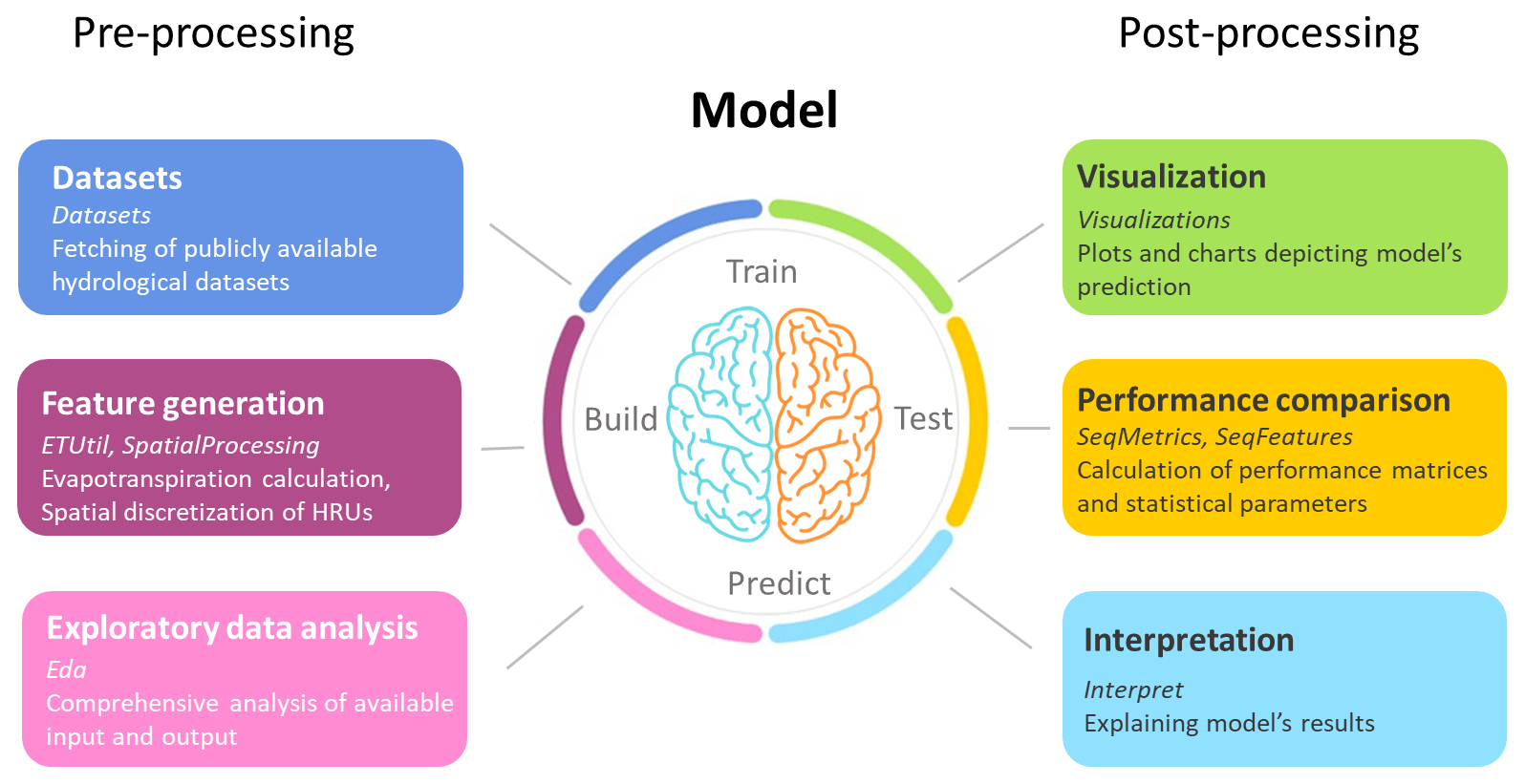
Figure 1Conceptual framework of hydrological modeling using AI4Water. AI4Water consists of modules for pre-processing and post-processing. The names of the modules are written in italics. The pre-processing steps involve collecting data, conducting exploratory data analysis on data, and generating new features from the data. The core of the model consists of building, training, and predicting. After this step, the predicted steps are used for visualization, performance comparison, and model interpretation.
The Model class of AI4Water has two implementations and can have three back ends. The two implementations are “model-subclassing” and “functional.” The back ends are either TensorFlow, PyTorch, or neither of them. The back ends, together with the implementations, determine the attributes that the Model class will inherit upon its creation. In the model-subclassing implementation, the Model class inherits from either the TensorFlow's Model class or the nn.module of PyTorch. This implementation allows all the attributes from the corresponding back end to be also available from AI4Water's Model class. For example, the “count_params” attribute of TensorFlow's Model class can also be obtained from the AI4Water's Model class. In functional implementation, the Model class of AI4Water does not inherit from the parent modules of TensorFlow/PyTorch. In this case, the built TensorFlow/PyTorch model object is displayed to the user as a “_model” attribute of the Model class. This is similar to TensorFlow and PyTorch libraries, both of which also have model-subclassing and functional implementations. For models other than TensorFlow or PyTorch, the Model class does not have any back end. In these cases, the machine learning models are built using libraries such as scikit-learn, XGBoost, CatBoost, or LightGBM. The built model object is exposed to the user as “_Model” attribute of the Model class.
The success of machine learning is proportional to testing various hypotheses by training and testing machine learning models and analyzing the results (Zaharia et al., 2018). This can quickly lead to a large number of output files. AI4Water handles this by automatically saving all the model-related files starting from model creation to pre-processing until the post-processing of each output in the respective folders. A detailed output directory structure is shown in Fig. 2. Upon every model run, a directory is created whose name is the date and time when the model is created. This naming convention allows for a simple and distinct directory structure for every new model. This parent directory is called “model path” and contains several sub-folders and files which are related to model configuration, model training, and the post-processing of results (Fig. 2a). The results for each target variable are saved in a separate folder. Additionally, the files related to the model's optimized parameters and interpretations are saved in a separate directory. The saved configuration file along with the weights can later be used to reproduce the model's results. In the case of hyperparameter optimization, a directory named “hpo path” is created, which consists of several “model paths”. Each of these “model paths” correspond to each iteration of the optimization algorithm (Fig. 2b). In the case of experiments, when different models are compared, a separate “hpo path” is created for each of the models being compared. Figure 2c shows the output file structure for an experiment when different machine learning algorithms are compared. This ordered arrangement of results facilitates the fast comparison and analysis of the results.

Figure 2Output directory structure of AI4Water. A “model path” (a) is created upon creation of a new model. An “hpo path” (b) is created during hyperparameter optimization. An “exp path” (c) is created when several models are compared during an experiment. The “hpo path” consists of several “model paths”, and an “exp path” consists of several “hpo paths”.
The code architecture of AI4Water, that is, its sub-submodules, their available classes, and third-party libraries, are illustrated in Fig. 3. AI4Water comprises 11 sub-modules, among which 10 are task-based, and one is a general-purpose module named “utils”. These sub-modules can be divided into two categories. The sub-modules on the left-hand side of Fig. 3 are designed for model building, hyperparameter optimization, and model comparison, whereas those on the right-hand side perform pre-processing and post-processing. Each sub-module exposes one or more classes to the user. For example, the HyperOpt sub-module presents the “Real”, “Categorical”, “Integer”, and HyperOpt classes. The third-party libraries required for each sub-module are annotated inside them. There are five “generic” third-party libraries that are required in all sub-modules (lower part of Fig. 3). The “et” and utils sub-modules do not require specific third-party libraries and depend only on generic libraries. The arrows in Fig. 3 indicate interaction between the sub-modules. The origin of the arrow denotes the caller sub-module, whereas their end points denote the sub-module that is being called. The Model class interacts with the pre-processing and post-processing modules using its functions, the names of which are shown in green in Fig. 3. For example, the “DataHandler” class in the pre-processing sub-module is responsible for data preparation. The Model class interacts with DataHandler using “training_data”, “validation_data”, and “test_data” methods. These methods are responsible for fetching training, validation, and test data from the DataHandler class, respectively.

Figure 3Framework architecture, sub-modules, classes, and third-party libraries used by AI4Water. Each box represents a sub-module. The names of classes in each sub-module are written along with the corresponding box. The third-party libraries upon which the sub-module depends are written inside the box. Empty boxes show that these sub-modules do not depend on a specific third-party library. The five generic libraries written at the bottom are used in all sub-modules. Arrows represent the caller sub-module and the sub-module being called. The sub-modules on the right-hand side are related to pre-processing and post-processing. The Model class interacts with pre-processing and post-processing sub-modules using its methods which are written in the green color.
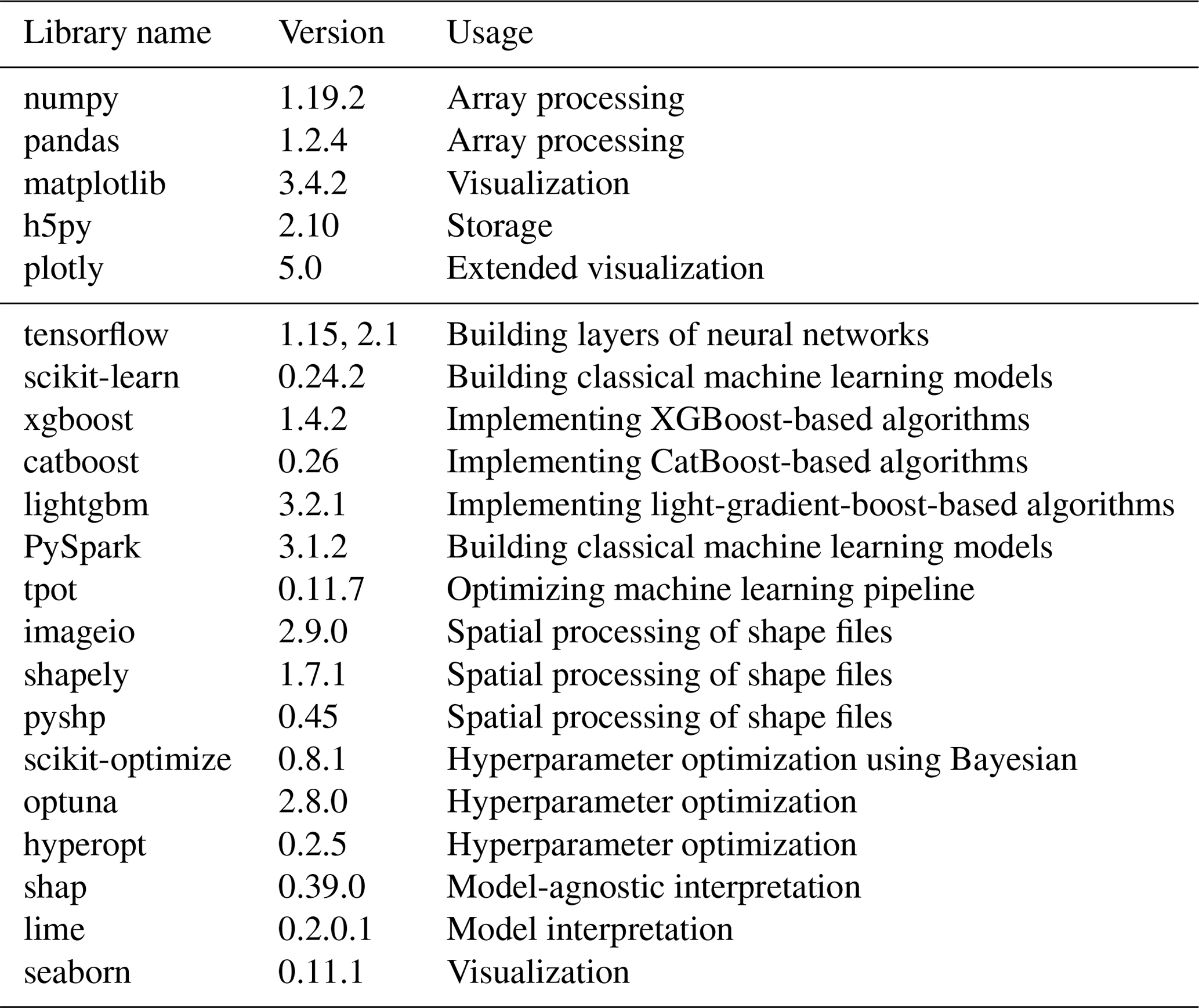
The large number of utilities in AI4Water increases the number of underlying libraries. The Model class is built on top of the scikit-learn, CatBoost, XGBoost, and LightGBM libraries to build classical machine learning models. These models have been used in several hydrological studies (Huang et al., 2019; Ni et al., 2020; Shahhosseini et al., 2021). To build deep learning models using neural networks, AI4Water uses popular deep learning platforms, such as TensorFlow (Abadi et al., 2016) and PyTorch. A complete list of the dependencies for AI4Water is presented in Table 1. It is divided into two parts. The first half shows the minimal requirements for running the basic utilities, which include building and training the model and making predictions from it. The second part of Table 1 comprises an exhaustive list of dependencies. These dependencies are required to utilize all functionalities of AI4Water. However, these utilities are optional and do not hamper the basic package functionality. Moreover, the modular structure of AI4Water allows the user to install libraries corresponding to a particular sub-module while ignoring the others which are not required. For example, in order to use the HyperOpt class for hyperparameter optimization, libraries related to post-processing are not required. Table 1 also presents the exact version of the underlying libraries which were used to test the 1.0 version of AI4Water. AI4Water handles the version conflicts of the underlying libraries, thereby making it version-independent. This implies that the user can use any version greater than the version number provided in Table 1.
Table 1Complete list of third-party Python libraries which are used by AI4Water. The first half the table enlists those libraries which are required, while the second half consists of those libraries which are optional.
3.1 Datasets
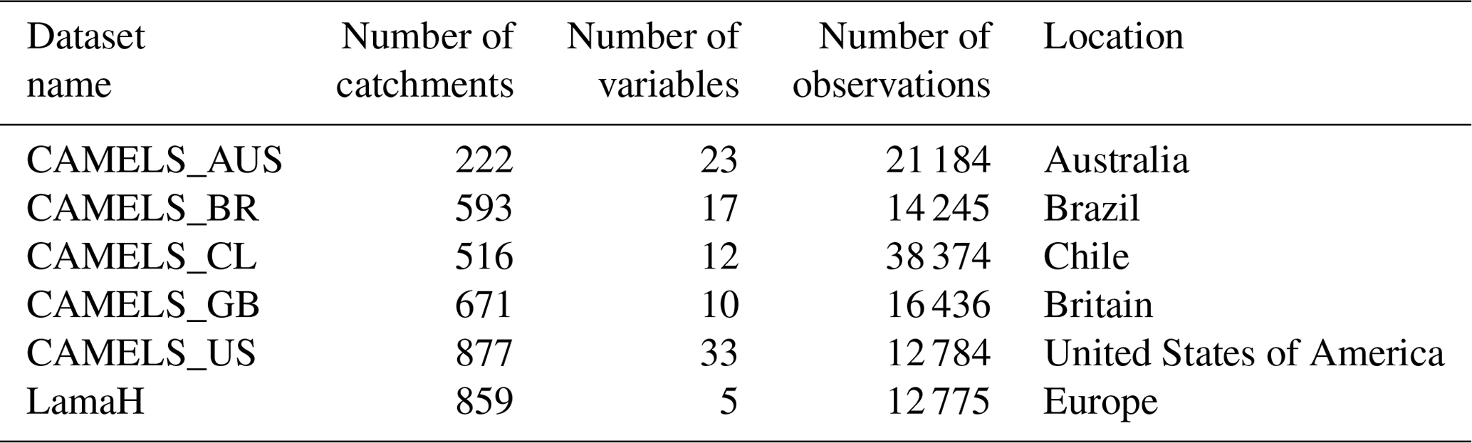
The first step in building a data-driven hydrological model is to obtain the data. There have been several efforts by the hydrological science community to build hydrological datasets that are publicly available. For example, for rainfall–runoff modeling, there exists the CAMELS dataset for several countries (Addor et al., 2017). The CAMELS dataset consists of daily weather data and streamflow records for multiple catchments. Another large rainfall–runoff dataset is LamaH (Klingler et al., 2021), which consists of observations from 859 catchments in Europe. While the number of such open-source datasets is large, the use of these data sources is slow as each database is available on different platforms and implements a different application programming interface (API). A core function of AI4Water is to provide a simple and homogeneous API to feed these datasets directly into machine learning models. Figure 4 shows the usage of the CAMELS_AUS dataset, in which the user needs to define only the name of the dataset and the input and output variables. This simple interface will help exploit the use of these datasets. Furthermore, benchmarking open-source datasets will likely accelerate the progress of machine learning in hydrological science. A brief summary of the rainfall–runoff datasets available in AI4Water is given in Table 2.
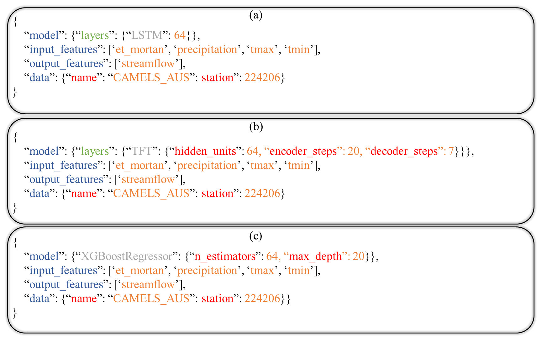
Figure 4Examples of declarative model definition in a config.json file. Panel (a) shows an example of an LSTM-based model using the CAMELS_AUS data (Fowler et al., 2021). Panels (b) and (c) show contents of configuration file for using temporal fusion transformer (Lim et al., 2021) and XGBoost (Chen and Guestrin, 2016) for rainfall–runoff modeling using CAMELS_AUS data, respectively.
Table 2Name and attributes of open-source datasets included in AI4Water.
3.2 Exploratory data analysis
A crucial step in data-driven hydrological modeling workflow is the visualization of the data. This step assists in understanding the data, finding outliers, selecting relevant features, and guiding the machine-learning-based modeling process. AI4Water provides an “eda” sub-module which can be employed to conduct a comprehensive analysis of input and output data. For example, the correlation plots illustrate the input variables which are more correlated with each other. Heat maps show the amount and position of the missing values. Histogram and box–whisker plots depict the distributions of both the input and output variables. This sub-module can also perform a principal component analysis of the input data and plot the principal components. This helps in understanding the dynamics of the input data and filtering the relevant features.
3.3 Pre-processing
3.3.1 Transformations
Data transformation includes standardizing and transforming the data onto a different scale. Transforming the data can significantly affect the performance of a data-driven model. The scikit-learn library provides several transformation functions such as “minmax”, “standardscaler”, “robust”, and “quantile”. Additionally, several decomposition methods such as empirical mode transformation (EMD), ensemble EMD (EEMD), wavelet transform (Sang, 2013), and fast Fourier transform (Sang et al., 2009) were found to improve the performance of hydrological models. AI4Water provides a uniform interface for all of these transformation methods under the sub-module “Transformations”. The user can apply any of the available transformations to any of the input features by using a simplified and uniform interface. The predicted features are transformed back after the prediction. Figure 5 shows a comparison of different transformations using a Taylor plot (Taylor, 2001). These results were generated by modeling in-stream E. coli concentrations in a small Laotian catchment (Boithias et al., 2021) using LSTM (Hochreiter and Schmidhuber, 1997). The input data were precipitation, relative humidity, air temperature, wind speed, and solar radiation.
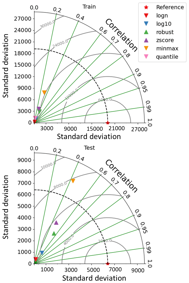
Figure 5Comparison of different transformations of output data on the performance of a neural network in the simulation of in-stream E. coli concentrations (most probable number, MPN, 100 mL) in a watershed in the Lao People's Democratic Republic.
3.3.2 Imputation
Missing values are often found in real-world datasets. However, missing data cannot be fed to machine learning algorithms. AI4Water provides various solutions for handling missing data that can be used using the “impute” method. These include using either the (1) pandas library (Mckinney, 2011), (2) scikit-learn library-based methods, or (3) dedicated algorithms to fill the missing input data. The pandas library allows the handling of missing values either by filling the missing values using the “fillna” method or interpolating the missing values using the “interpolate” method. Both these methods can be seamlessly used with the impute method in AI4Water. Several imputation methods for filling missing values are available in the scikit-learn library. These methods include “KNNImputer”, “IterativeImputer”, and “SimpleImputer”. AI4Water provides a uniform interface for all imputation methods without hindering their functionality.
Several other libraries have been developed that have dedicated algorithms for imputing missing time series data. These include “fancyimpute” (Rubinsteyn and Feldman, 2016) and “transdim” (X. Chen et al., 2020). The fancyimpute library provides several state-of-the-art algorithms such as “SoftImpute” (Mazumder et al., 2010), “IterativeSVD” (Troyanskaya et al., 2001), “MatrixFactorization”, “NuclearNormMinimization” (Candès and Recht, 2009), and “Biscaler” (Hastie et al., 2015). The transdim library provides algorithms based upon neural networks for filling missing data. AI4Water provides a simple interface for using these libraries with their full functionalities using the impute method.
3.3.3 Missing labels
In supervised machine learning problems, the training data consist of examples. Each example consists of one or more input data points and a corresponding label, which is the true value for the given example. Similar to the input data, it is common for the labels to have missing data. Although the missing values in target features can be handled similarly to those of input features, which has been explained in Sect. 2.3, this can lead to unrealistic results, particularly when the number of missing values is large. AI4Water allows the user to exclude examples with missing labels during model training. For multi-output prediction, one can encounter situations in which all target variables are not available for a given example. AI4Water allows the user to handle such situations by masking the missing observations during loss calculation. However, the user can also opt to exclude these examples, although this can reduce the number of examples in water quality problems in which the number of samples is already very small.
3.3.4 Resampling
Modeling hydrological processes at high temporal resolutions can result in a large amount of data (Li et al., 2021). Training with this large input data can be computationally expensive. However, temporally coarse input data contain little information. AI4Water handles large amounts of data by either resampling the data at a lower temporal resolution using the “Resample” class or by skipping every nth input data, where n represents the time step. The latter can be achieved by setting the “input_steps” argument to a value >1. The default value of this argument is 1, which results in the use of all input data.
3.3.5 Feature generation
The incorporation of scientific knowledge into machine learning models is an emerging paradigm for constraining predictions from machine learning models to reality (Wang et al., 2020). The guiding principle of AI4Water is to integrate domain-specific knowledge and hydrological data. AI4Water automates the calculation of several features and their inputs to the machine learning algorithm. The input data requirement for the calculation of these features is minimal as they are calculated from the raw data. The calculated features are in the form of a time series, which are then directly given as input to machine learning algorithms. The following sections describe the feature generation process in more detail.
Land use change and HRU discretization
In rainfall–runoff modeling, the method of discretization of the HRU plays an important role in many theory-driven models such as the Soil and Water Assessment Tool (SWAT) (Neitsch et al., 2011) and Hydrological Simulation Program FORTRAN (HSPF) (Bicknell et al., 1997). An HRU is a building block of a process-driven hydrological model in which all the processes are simulated. The area and formation of an HRU depend on its definition. For example, in the HSPF model, an HRU is defined as a unique land use in a unique sub-basin. On the other hand, the SWAT model considers slope classes and soil type distributions in an HRU. In catchments, which undergo changes in land use over time, the corresponding HRUs also change with time. Temporal changes in HRUs are a major challenge in most process-driven models (Kim et al., 2018). However, it has been shown that machine learning models can easily incorporate land use changes with time and dynamic HRU calculations (Abbas et al., 2020). AI4Water contains a sub-module “MakeHRUs”, which helps in distributing the time series of weather data into HRUs using different HRU definitions. Figure 6 shows two discretization schemes that combine land use, soil type, and sub-basin. However, the user can also add other spatially varying features, such as slope, in the HRU definition. A complete list of the HRU definitions is provided in Table S1 in the Supplement. Figure 7 illustrates the HRU variation with time in a Laotian catchment (Abbas et al., 2020). The HRUs shown in Fig. 7 are defined as a unique land use with a unique soil type. Thus, every HRU has distinct land use and soil characteristics. As there are four land use types and three soil types in the catchment, the total number of HRUs was 12. We can observe how the area of certain HRUs, e.g., “Alisol_Fallow”, decreases with time at the expense of other HRUs (Fig. 7a). The relative contributions of each HRU for the years 2011, 2012, 2013, and 2014 is illustrated in Fig. 7b–e, respectively. The MakeHRUs sub-module requires shapefiles of land use, soil, and slope to make the HRU according to a given definition.
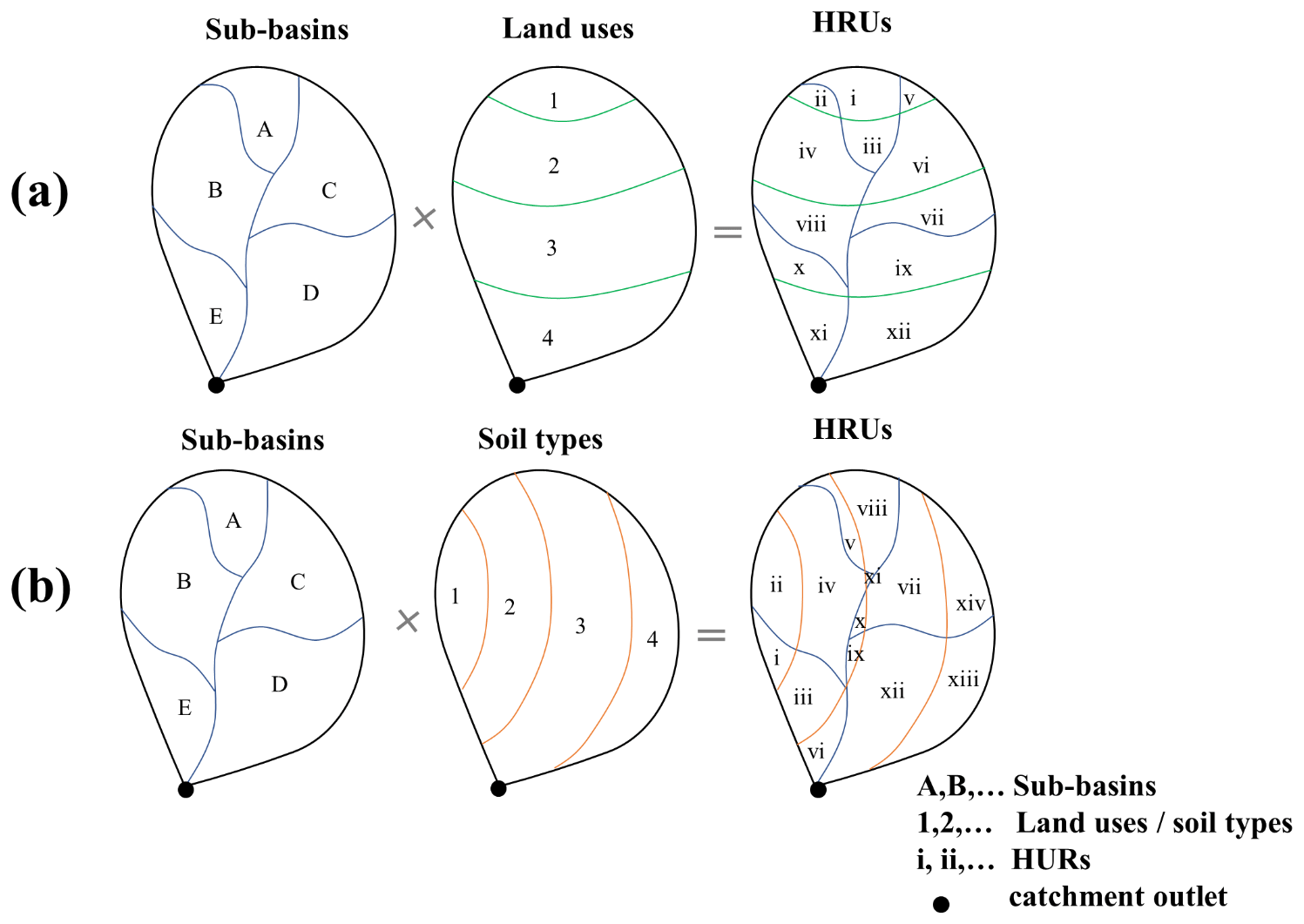
Figure 6Example of HRU discretization schemes by combining (a) sub-basins and land uses and by combining (b) sub-basins and soil types.

Figure 7Discretization of a catchment in Laos (Boithias et al., 2021) according to the HRU definition of “unique land use in unique soil”. The catchment consists of three soil types and four land use types. The soil types are Alisol, Luvisol, and Leptosol, while the land use types are fallow, forest, teak, and crop. The combination of soil types and land use types results in 12 distinct HRUs. Panel (a) shows annual variation in these 12 land use types, while (b)–(e) show the percentage area of HRUs in the catchment in 2011, 2012, 2013, and 2014, respectively.
3.3.6 DataHandler class
The DataHandler class prepares the input data for the machine learning model and acts as an intermediate between the Model class and other pre-processing classes, such as “Imputation” and “Transformation” classes. The DataHandler can read data from various files as long as the data are in a tabular format in those files. The complete list of allowed file types and their accepted file extensions is provided in Table S5 in the Supplement. Internally, the DataHandler class stores data as a pandas “DataFrame” object, which is a data model of pandas for tabular data (Mckinney, 2011). DataHandler can also save processed data as an HDF5 file, which can be used to inspect processed input data.
3.4 Evapotranspiration
The amount of evapotranspiration is an important factor that affects the total water budget in a catchment. The impact of the evapotranspiration process representation in rainfall–runoff models has been studied extensively (Guo et al., 2017). Several potential and reference evapotranspiration calculation methods are available in the literature. AI4Water contains sub-module “et” which can be used to calculate the potential evapotranspiration using various methods. These include complex methods such as Penman–Monteith (Allen et al., 1998), which require many input variables, and simplified methods such as Jensen and Haise (Jensen and Haise, 1963), which only depend on temperature. The “et” can furthermore calculate potential evapotranspiration at various time intervals, from 1 min to 1 year. The names of the 22 evapotranspiration methods available in “et” and their data requirements are summarized in Table S2 in the Supplement. The CAMELS Australia dataset (Fowler et al., 2021) comes with pre-calculated potential evapotranspiration using the Morton (Morton, 1983) method. We compared this method with three different potential evapotranspiration calculation methods using “et”, as depicted in Fig. 8.
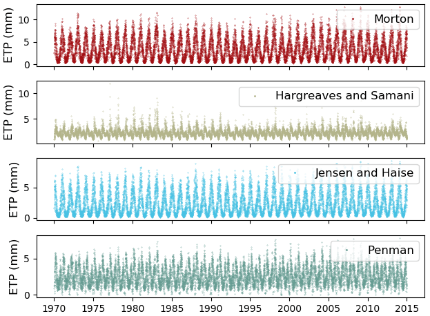
Figure 8Comparison of various evapotranspiration methods for the CAMELS_AUS dataset. The CAMELS_AUS dataset comes with the Morton method, while the remaining three methods are calculated by the “et” sub-module of AI4Water.
3.5 Hyperparameter optimization
The hyperparameters of a machine learning algorithm are the parameters that remain fixed during model training and significantly influence its performance (Chollet, 2018). Thus, the choice of hyperparameters plays an important role in evaluating the performance of machine learning algorithms. Some of the most popular approaches for optimizing hyperparameters are random search, grid search, and the Bayesian approach. Random search involves randomly selecting parameters from the given space for a given number of iterations. Grid search, on the other hand, comprehensively explores all possible combinations of hyperparameters in the hyperparameter space. Although grid search can ensure global minima, the number of iterations increases exponentially with an increase in the number of hyperparameters. This renders the grid search practically unfeasible for deep-neural-network-based models, which are computationally expensive. The two commonly used Bayesian approaches are Gaussian processes (Snoek et al., 2012) and the tree-structured Parzen estimators (TPEs) (Bergstra et al., 2011).
The libraries used to implement these algorithms are HyperOpt (Bergstra et al., 2013), “scikit-optimize” (Head et al., 2018), “optuna” (Akiba et al., 2019), and scikit-learn (Pedregosa et al., 2011). These libraries implement different algorithms with different strengths. The scikit-optimize library allows the application of the Bayesian optimization approach using Gaussian Processes. The scikit-learn library can be used for random and grid-search-based approaches. The HyperOpt module assists in Bayesian optimization using TPEs. The HyperOpt sub-module in AI4Water provides a uniform interface to interact with all of the aforementioned libraries. The integration of HyperOpt with its underlying modules not only complements the underlying optimization algorithms but also adds additional functionality, such as visualization. For example, the importance of hyperparameters is plotted using the functional analysis of variance (FANOVA) method proposed by Hutter et al. (2014).
We demonstrate the use of the HyperOpt sub-module of AI4Water for optimizing the hyperparameters of an LSTM-based neural network for rainfall–runoff modeling. The input data consisted of climate data, whereas the target was streamflow. For this example, we used CAMELS data from a catchment in Australia (Fowler et al., 2021). We compared the performance of random search, grid search, and two Bayesian algorithms based on Gaussian processes and TPEs. The convergence plots of all four algorithms are shown in Fig. 9. The Bayesian approach using Gaussian processes was found to be the most useful for minimizing the objective function. The objective function was the minimum of the validation loss. We also observed that grid search, despite a large number of iterations, did not perform better than the other three methods.
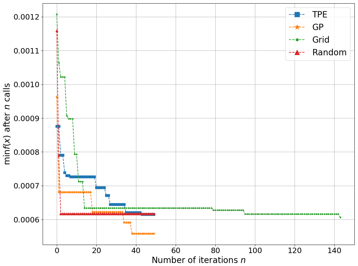
Figure 9Comparison of four optimization algorithms for optimizing hyperparameters of an LSTM-based model for rainfall–runoff modeling. GP represents Bayesian with Gaussian processes, while TPE stands for tree-structured Parzen estimator. Grid and random stand for grid-search- and random-search-based optimization, respectively. The x axis shows the number of function evaluations, while minf(x) on the y axis represents the objective function, which takes x hyperparameters and returns the minimum of validation loss.
3.6 Model comparison with Experiment
AI4Water consists of an Experiment sub-module, which makes it easier to compare different machine learning models. The basic purpose of the Experiment class is to compare different models by optimizing their hyperparameters. This is made possible as the Experiment class encompasses the HyperOpt class, which in turn encompasses the Model class (Fig. 10). Thus, the Experiment class can be used for combined algorithm selection and hyperparameter optimization (Thornton et al., 2013). The results from the Experiment class are organized within an “exp path” directory (Fig. 2). The Experiment class can be sub-classed to compare any number and type of models. It consists of three sub-classed experiments: “MLRegressionExperiment”, “MLClassificationExperiment”, and “TransformationExperiment”. The MLRegressionExperiment class runs and compares approximately 50 different classical machine learning algorithms for a regression task. The MLClassificationExperiment class compares classical machine learning algorithms for a classification problem. The TransformationExperiment class can be used to compare the application of different transformation techniques (Sect. 3.3.1) on different input and output features.

Figure 10Hierarchy of model building and comparison in AI4Water. The Model class involves building, training, and prediction. The hyperparameter optimization step iterates over the Model class until the best hyperparameters are obtained. Experiments are then designed to compare the performance of different model architectures after tuning their hyperparameters.
We conducted an experiment to compare the performance of classic machine learning algorithms in predicting antibiotic-resistant genes (ARGs) at a recreational beach (Jang et al., 2021). The results of this experiment are shown in Fig. 11, which compares the correlation coefficients for the training and test sets. It can be seen that some algorithms can yield an R2 as high as 0.65. Other algorithms provide training R2 as high as 1.0, which indicates overfitting. In particular, we observed strong overfitting in the case of the decision tree regressor and Gaussian process regressor. It can also be inferred from Fig. 11 that ensemble methods such as AdaBoost (Freund and Schapire, 1997), gradient boosting (Friedman, 2001), bagging (Ho, 1998), extra trees (Geurts et al., 2006), and random forest (Liaw and Wiener, 2002) yield better performance than other methods. We also observed that simple linear models such as LARS (least-angle regression), Lasso, and multi-layer perceptron are not able to model the dynamic and complex functions of the ARG distribution at the beach. On the other hand, complex nonlinear models such as CatBoost (Prokhorenkova et al., 2017), XGBoost (Chen and Guestrin, 2016), and light gradient boosting machines (Ke et al., 2017) are able to adequately capture dynamic features related to the ARG distribution. We also observed that algorithms with cross-validation performed better than their counterparts without cross-validation.
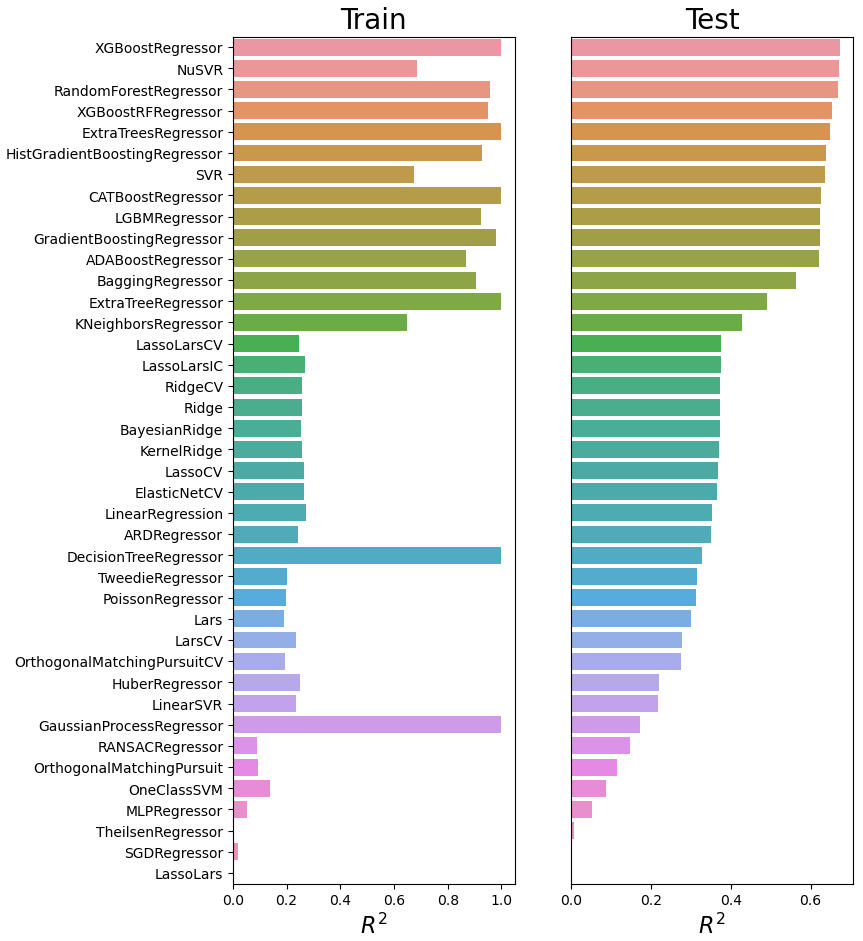
Figure 11An experiment which compares ARG prediction performance at a recreational beach in Korea using various machine learning algorithms. The y axis represents abbreviations of the algorithms. The complete names of algorithms are given in Table S4 in the Supplement. The hyperparameters of each of the algorithms were optimized during the experiment.
3.7 Post-processing
The post-processing submodule of AI4Water consists of several utilities which can be used once the machine learning model has been trained. These utilities are discussed in detail below.
3.7.1 Visualization
The “visualize” sub-module, consisting of a “Visualize” class, is used to examine inside the machine learning model. When the model comprises several layers of neural networks, this class plots the outputs of the intermediate layers, gradients of these outputs, weights and biases of intermediate layers, and gradients of these weights. Thus, this class helps to visualize the working of neural networks. It can also be used to plot the decision tree learned by the tree-based machine learning model. We demonstrate the use of this class by building a four-layer neural network to predict streamflow using the CAMELS dataset (Fowler et al., 2021). The four-layered neural network comprises an input layer, two layers of LSTM, and a dense layer as output layer (Fig. S1 in the Supplement). The dense layer is a fully connected layer which is used for dimensionality reduction (Chollet, 2018). Figures S2–S5 in the Supplement show the outputs of the first LSTM layer and its gradients along with the weights of the first LSTM layer, as well as the gradients of those weights.
3.7.2 Interpretation and explainable AI
The interpretation of the results of machine learning models is an area of active research. For classical machine learning algorithms, interpretation tools include the plotting of decision trees or input feature importance. For neural-network-based models, explainability is considered an even bigger challenge. AI4Water consists of a sub-module called “Interpret”, which can be used to plot interpretable results. The Interpret class takes the trained model of AI4Water as input and plots numerous results which help to explain the behavior of the model. The exact type of plots generated by the Interpret sub-module depends on the algorithm used by the model. For neural-network-based models, which consist of a layered structure, the Interpret sub-module plots all the trained weights, the outputs of each layer, the gradients of weights, and the gradients of the activations of neural networks. This also includes plotting attention weights if the model consists of an attention mechanism. AI4Water automatically plots the results of the model when a model is used for prediction. These include the scatter and line plots of each target variable.
We demonstrate this by using a dual-stage attention model (Qin et al., 2017) for daily rainfall–runoff modeling in catchment number 401 203 in the CAMELS Australia dataset (Fowler et al., 2021). The input data consisted of evapotranspiration, precipitation, minimum and maximum temperatures, vapor pressure, and relative humidity. The dual-stage model showed significant performance during training (R2=0.93) and test (R2=0.87), as shown in Fig. S6 in the Supplement. The dual-stage attention model highlights the importance of the input variables for prediction. The attention weights for each of the input variables are shown in Figs. S7–S9 in the Supplement. From these figures, we can infer that the highest attention is given to precipitation followed by evapotranspiration. Furthermore, we also observed that the input of the previous 3–4 d was the most important. This can be attributed to the higher attention weights during the first 3–4 look-back steps in these figures. We also observed periodic changes in attention weights for all input variables, which can be attributed to the seasonal variations of input variables.
Several model-agnostic methods have recently been developed to explain black-box machine learning models, such as local independent model explanations (LIMEs) (Ribeiro et al., 2016) and shapely additive explanations (SHAPs) (Lundberg and Lee, 2017). These methods explain the behavior of complex machine learning models (such as black-box) using a simplified but interpretable model. However, using these methods in high-stakes decision-making has been criticized (Rudin, 2019). The explanations of these methods can be local or global. A local explanation describes the behavior of the model for a single example, whereas a global explanation can describe the model's behavior for all examples. The LIME method is only relevant for local explanations, whereas SHAP also provides explanations for approximating the global importance of a feature. AI4Water consists of “LimeExplainer” and “ShapExplainer” classes to explain the behavior of a machine learning model using the LIME and SHAP methods, respectively.
We built an XGBoost (Chen and Guestrin, 2016) model for the prediction of E. coli in a Laotian catchment (Boithias et al., 2021). Figure S10 in the Supplement shows the output of the LimeExplainer class, whereas Fig. S11 in the Supplement shows the output of the ShapExplainer class. In Fig. S10, a large horizontal bar for a given feature indicates that this feature strongly affected the model's prediction. A positive value indicates that the given feature caused an increase in the model's prediction. On the other hand, the negative value indicates that it caused a decrease in the model's prediction. Thus, large negative values for solar radiation in example 41 indicate that the solar radiation causes a large reduction in the model's prediction. Large positive values for water level in examples 42 to 46 indicate that the water level in these cases strongly increased the model's prediction. The numerical values of features along the y axis indicate which value of feature was responsible for the aforementioned behavior. Thus, more precisely, the water level above 147.8 cm causes a very large increase in the model's prediction. Therefore, we can verify that the E. coli predictions during flood events are more strongly affected by water level.
The SHAP module provides a more detailed explanation about the local and global importance of input features on the model's prediction. Figure S11a and b show the local explanation summary of the model in the form of the SHAP value of each input feature for each example (Lundberg et al., 2020). Figure S11a shows that the examples with large SHAP values of water level and suspended matter resulted in large E. coli predictions. The f(x) in Fig. S11a indicates the sum of SHAP values of all input features. The prediction of the machine learning model is equal to the sum of f(x) and the base value. The base value is the mean of the total predictions from the model on training data (Lundberg et al., 2018). In our example the base value was 4661.082 MPN 100 mL−1 (MPN signifies most probable number). The examples in Fig. S11a are clustered in such a way that examples with similar explanations are grouped together. Figure S11b indicates that the large values of water level and suspended particulate matter result in an increase in E. coli. On the other hand, large values of solar radiation resulted in negative SHAP values. This shows that large solar radiation causes a reduction in E. coli prediction. Figure S11c shows the global importance of input features for E. coli prediction. This global importance is obtained by calculating the mean of the SHAP value of a feature for all examples (Lundberg and Lee, 2016). The explanations from Fig. S11 correlate with our background understanding of E. coli behavior. Several studies have shown that E. coli in surface water is strongly affected by suspended solids, water level, and solar radiations (Nakhle et al., 2021; Pandey and Soupir, 2013).
3.7.3 Performance metrics
Performance metrics are a vital component of the evaluation framework for machine learning (Botchkarev, 2018). There are two major types of performance metrics related to the evaluation of a model's forecasting ability. These include scale-dependent and scale-independent error metrics. Scale-dependent metrics, such as mean absolute error, provide a good estimate of a single model's performance, but they cannot be used across the models because of their scale dependency (Prestwich et al., 2014). Scale-independent error metrics are more useful when comparing the performance of various models (Hyndman and Koehler, 2006). However, certain scale-independent error metrics cannot be defined when one or more observed values are zero, such as percentage errors or relative errors (Hyndman, 2006). The choice of a performance metric to evaluate the model depends on the problem definition and model objectives (Wheatcroft, 2019). AI4Water calculates over 100 regression metrics and numerous classification metrics to help the user analyze the general characteristics of the forecasts. These performance metrics are sub-packaged under SeqMetrics in AI4Water. These metrics are calculated automatically for all the target variables whenever a model is used for prediction using the “predict” method. The metrics are stored in a json file inside the path of the model (errors.json in Fig. 2). The names of the performance metrics calculated by AI4Water are listed in Table S3 in the Supplement. Additionally, several statistical parameters of the predicted variable were calculated and stored in this json file.
All features of AI4Water can be accomplished using a configuration file. The configuration file (config.json) of AI4Water consists of a human-readable json file. All the information regarding pre-processing of data, building and training of the model, predictions, and post-processing of results is written in this file. This file is generated every time a new model is built. One of the advantages of this configuration file is that any user can build and run the models without having to write the code explicitly. All examples presented in this study can be run using the corresponding configuration files. Figure 4 shows three examples of configuration files. Figure 4a shows an LSTM-based model built for rainfall–runoff modeling using the CAMELS (Fowler et al., 2021) dataset. Figure 4b and c show the usage of the temporal fusion transformer and XGBoost models for the same task. The user can define commands to control the input and output features to use or the training duration for the model. All hyperparameters of the model can also be set using this configuration file.
AI4Water was built using the object-oriented programming (OOP) paradigm. Its core logic was implemented by the Model class. The use of OOP allows a user to customize any steps of model building, training, or testing by sub-classing the Model class. This may include the implementation of a custom training loop or a customized loss function. Similarly, the pre-processing and data preparation steps implemented in the Model class can also be overwritten for specific usages. For example, if users want to implement another transformation on the training data, they can sub-class the Model class and overwrite the training_data method. Similarly, the user can customize the loss function by overwriting the “loss” method of the Model class. Additionally, AI4Water exposes the underlying machine learning libraries such as TensorFlow and scikit-learn to the user. Thus, users can directly use these libraries and implement the desired configuration. However, this requires a deeper understanding of the underlying libraries.
AI4Water version 1.0 was tested with continuous integration tools with GitHub Actions to ensure that it passes all the written tests and can be installed on computers. The tests were conducted on Windows- and Linux-based operating systems. In addition, we tested the package on Python versions 3.6, 3.7, and 3.8. The package was also tested with TensorFlow versions 1.15 and above.
-
The current version of AI4Water was designed only for supervised learning problems. However, there has been growing interest in unsupervised machine learning models, such as generative adversarial networks (GANs) and reinforcement learning. GANs have been shown to exhibit high performance for time-series-related tasks such as filling missing data (Luo et al., 2018) or generating new high-resolution data (Chen et al., 2019). This aspect of GANs can be useful in water quality modeling, in which data collection is costly and missing observations are common. Reinforcement learning can be applied to optimal policy design in hydrological systems, such as scheduling the release of water from a dam (Sit et al., 2020).
-
Another limitation of AI4Water is its dependence on a large number of third-party libraries. This can be challenging during installation when the interdependencies of libraries conflict with each other. Although we have provided the exact versions of the third-party libraries, which were used to test the current version of AI4Water, a conflict in future due to the changes in third-party libraries cannot be guaranteed. As AI4Water is an open-source project, we consider that such conflicts can be minimized with community inputs.
-
AI4Water was designed for the rapid testing and experimentation of deep learning models. However, it should be noted that the current version of the framework is not suitable for the deployment of deep learning models in production.
-
As all the options to use AI4Water are accommodated in a configuration file, this makes it suitable for developing a graphical user interface (GUI). Adding GUIs will further widen the user base of AI4Water by being accessible to non-programmers.
Modeling hydrological processes by machine learning requires the development of pipelines that encompass data retrieval, feature extraction, visualization, and building, training, and testing the machine learning model, along with visualization and interpretation of the results. The AI4Water software introduced in this work was designed to facilitate the development, reuse, and reproducibility of machine learning models for applications in hydrology. AI4Water was designed to integrate the domain-specific aspects of hydrological modeling with the professional level of machine learning and data processing software already developed and used by the Python community. We demonstrated the applicability of AI4Water with supervised learning examples related to hydrological modeling. Further development of the package is suggested with new features that may make AI4Water more versatile. The platform is expected to be practical for a wide range of users interested in hydrological modeling.
The AI4Water source code can be found in a publicly available GitHub repository (https://github.com/AtrCheema/AI4Water, last access: 18 March 2022), and its version 1.0 is archived at https://doi.org/10.5281/zenodo.5595680 (Abbas et al., 2021). The user manual is built into the source code “Docstring” and compiled into a “read the docs” web page (https://ai4water.readthedocs.io/en/latest/, last access: 18 March 2022) using Sphinx (Brandl, 2010) software. The Jupyter notebooks replicating the examples described in the paper are available in the “examples” directory.
The supplement related to this article is available online at: https://doi.org/10.5194/gmd-15-3021-2022-supplement.
AA was responsible for conceptualization, code development, and writing the draft. LB, YP, and KK were responsible for review and editing. JAC was responsible for review, editing, and supervision. KHC was involved in conceptualization, funding acquisition, supervision, review, and editing.
The contact author has declared that neither they nor their co-authors have any competing interests.
Publisher's note: Copernicus Publications remains neutral with regard to jurisdictional claims in published maps and institutional affiliations.
This study was supported by Basic Science Research Program through the National Research Foundation of Korea (NRF) funded by the Korean Ministry of Education (no. 2017R1D1A1B04033074), as well as the Korea Environment Industry and Technology Institute (KEITI) through the Aquatic Ecosystem Conservation Research Program funded by Korean Ministry of Environment (MOE) (no. 2020003030003). The authors also thank Campus France (PHC STAR 41510WH) for their financial support.
This study was supported by Basic Science Research Program through the National Research Foundation of Korea (NRF) funded by the Korean Ministry of Education (no. 2017R1D1A1B04033074). It was also supported by the Korea Environment Industry and Technology Institute (KEITI) through the Aquatic Ecosystem Conservation Research Program funded by Korean Ministry of Environment (MOE) (no. 2020003030003).
This paper was edited by Wolfgang Kurtz and reviewed by two anonymous referees.
Abadi, M., Barham, P., Chen, J., Chen, Z., Davis, A., Dean, J., Devin, M., Ghemawat, S., Irving, G., and Isard, M.: Tensorflow: A system for large-scale machine learning, in: 12th {USENIX} symposium on operating systems design and implementation ({OSDI} 16), 265–283, 2016.
Abbas, A., Baek, S., Kim, M., Ligaray, M., Ribolzi, O., Silvera, N., Min, J.-H., Boithias, L., and Cho, K. H.: Surface and sub-surface flow estimation at high temporal resolution using deep neural networks, J. Hydrol., 590, 125370, https://doi.org/10.1016/j.jhydrol.2020.125370, 2020.
Abbas, A., Iftikhar, S., and Kwon, D.: AtrCheema/AI4Water: AI4Water v1.0: An open source python package for modeling hydrological time series using data-driven methods (v1.0-beta.1), Zenodo [data set and code], https://doi.org/10.5281/zenodo.5595680, 2021.
Addor, N., Newman, A. J., Mizukami, N., and Clark, M. P.: The CAMELS data set: catchment attributes and meteorology for large-sample studies, Hydrol. Earth Syst. Sci., 21, 5293–5313, https://doi.org/10.5194/hess-21-5293-2017, 2017.
Akiba, T., Sano, S., Yanase, T., Ohta, T., and Koyama, M.: Optuna: A next-generation hyperparameter optimization framework, in: Proceedings of the 25th ACM SIGKDD international conference on knowledge discovery and data mining, 2623–2631, 2019.
Allen, R. G., Pereira, L. S., Raes, D., and Smith, M.: Crop evapotranspiration-Guidelines for computing crop water requirements-FAO Irrigation and drainage paper 56, Fao, Rome, 300, 1998.
Bergstra, J., Bardenet, R., Bengio, Y., and Kégl, B.: Algorithms for hyper-parameter optimization, Adv. Neur. In., 24, 2546–2554, 2011.
Bergstra, J., Yamins, D., and Cox, D.: Making a science of model search: Hyperparameter optimization in hundreds of dimensions for vision architectures, in: International conference on machine learning, 115–123, 2013.
Bicknell, B. R., Imhoff, J. C., Kittle Jr., J. L., Donigian Jr., A. S., and Johanson, R. C.: Hydrological simulation program – FORTRAN user's manual for version 11, Environmental Protection Agency Report No. EPA/600/R-97/080, US Environmental Protection Agency, Athens, GA, 1997.
Boithias, L., Auda, Y., Audry, S., Bricquet, J. P., Chanhphengxay, A., Chaplot, V., de Rouw, A., Henry des Tureaux, T., Huon, S., and Janeau, J. L.: The Multiscale TROPIcal CatchmentS critical zone observatory M-TROPICS dataset II: land use, hydrology and sediment production monitoring in Houay Pano, northern Lao PDR, Hydrol. Process., 35, e14126, https://doi.org/10.1002/hyp.14126, 2021.
Botchkarev, A.: Performance metrics (error measures) in machine learning regression, forecasting and prognostics: Properties and typology, arXiv [preprint], arXiv:1809.03006, 2018.
Brandl, G.: Sphinx documentation, http://sphinx-doc.org/sphinx.pdf (last access: 18 March 2022), 2010.
Burns, D. M. and Whyne, C. M.: Seglearn: A python package for learning sequences and time series, J. Mach. Learn. Res., 19, 3238–3244, 2018.
Candès, E. J. and Recht, B.: Exact matrix completion via convex optimization, Found. Comput. Math., 9, 717–772, 2009.
Chakraborty, M., Sarkar, S., Mukherjee, A., Shamsudduha, M., Ahmed, K. M., Bhattacharya, A., and Mitra, A.: Modeling regional-scale groundwater arsenic hazard in the transboundary Ganges River Delta, India and Bangladesh: Infusing physically-based model with machine learning, Sci. Total Environ., 748, 141107, https://doi.org/10.1016/j.scitotenv.2020.141107, 2020.
Chen, H., Zhang, X., Liu, Y., and Zeng, Q.: Generative adversarial networks capabilities for super-resolution reconstruction of weather radar echo images, Atmosphere, 10, 555, https://doi.org/10.3390/atmos10090555, 2019.
Chen, K., Chen, H., Zhou, C., Huang, Y., Qi, X., Shen, R., Liu, F., Zuo, M., Zou, X., and Wang, J.: Comparative analysis of surface water quality prediction performance and identification of key water parameters using different machine learning models based on big data, Water Res., 171, 115454, https://doi.org/10.1016/j.watres.2019.115454, 2020.
Chen, T. and Guestrin, C.: Xgboost: A scalable tree boosting system, in: Proceedings of the 22nd acm sigkdd international conference on knowledge discovery and data mining, 785–794, https://doi.org/10.1145/2939672.2939785, 2016.
Chen, X., Yang, J., and Sun, L.: A nonconvex low-rank tensor completion model for spatiotemporal traffic data imputation, Transport. Res. C-Emer., 117, 102673, https://doi.org/10.1016/j.trc.2020.102673, 2020.
Cheng, Y., Li, D., Guo, Z., Jiang, B., Lin, J., Fan, X., Geng, J., Yu, X., Bai, W., and Qu, L.: Dlbooster: Boosting end-to-end deep learning workflows with offloading data preprocessing pipelines, in: Proceedings of the 48th International Conference on Parallel Processing, 1–11, 2019.
Chollet, F.: Deep learning with Python, 1, Manning Publications Co., ISBN 9781617294433, 2018.
Christ, M., Braun, N., Neuffer, J., and Kempa-Liehr, A. W.: Time series feature extraction on basis of scalable hypothesis tests (tsfresh – a python package), Neurocomputing, 307, 72–77, 2018.
Collenteur, R. A., Bakker, M., Caljé, R., Klop, S. A., and Schaars, F.: Pastas: open source software for the analysis of groundwater time series, Groundwater, 57, 877–885, 2019.
Coxon, G., Addor, N., Bloomfield, J. P., Freer, J., Fry, M., Hannaford, J., Howden, N. J. K., Lane, R., Lewis, M., Robinson, E. L., Wagener, T., and Woods, R.: CAMELS-GB: hydrometeorological time series and landscape attributes for 671 catchments in Great Britain, Earth Syst. Sci. Data, 12, 2459–2483, https://doi.org/10.5194/essd-12-2459-2020, 2020.
Faouzi, J. and Janati, H.: pyts: A Python Package for Time Series Classification, J. Mach. Learn. Res., 21, 46:41–46:46, 2020.
Ferreira, L. B. and da Cunha, F. F.: New approach to estimate daily reference evapotranspiration based on hourly temperature and relative humidity using machine learning and deep learning, Agr. Water Manage., 234, 106113, https://doi.org/10.1016/j.agwat.2020.106113, 2020.
Fowler, K. J. A., Acharya, S. C., Addor, N., Chou, C., and Peel, M. C.: CAMELS-AUS: hydrometeorological time series and landscape attributes for 222 catchments in Australia, Earth Syst. Sci. Data, 13, 3847–3867, https://doi.org/10.5194/essd-13-3847-2021, 2021.
Freund, Y. and Schapire, R. E.: A decision-theoretic generalization of on-line learning and an application to boosting, J. Comput. Syst. Sci., 55, 119–139, 1997.
Friedman, J. H.: Greedy function approximation: a gradient boosting machine, Ann. Stat., 29, 1189–1232, https://doi.org/10.1214/aos/1013203451, 2001.
Geurts, P., Ernst, D., and Wehenkel, L.: Extremely randomized trees, Mach. Learn., 63, 3–42, 2006.
Guo, D., Westra, S., and Maier, H. R.: Impact of evapotranspiration process representation on runoff projections from conceptual rainfall-runoff models, Water Resour. Res., 53, 435–454, 2017.
Hastie, T., Mazumder, R., Lee, J. D., and Zadeh, R.: Matrix completion and low-rank SVD via fast alternating least squares, J. Mach. Learn. Res., 16, 3367–3402, 2015.
Head, T., MechCoder, G. L., and Shcherbatyi, I.: scikit-optimize/scikit-optimize: v0. 5.2, Zenodo [code], https://doi.org/10.5281/zenodo.5565057, 2018.
Ho, T. K.: The random subspace method for constructing decision forests, IEEE T. Pattern Anal., 20, 832–844, 1998.
Hochreiter, S. and Schmidhuber, J.: Long short-term memory, Neural Comput., 9, 1735–1780, 1997.
Huang, Y., Bárdossy, A., and Zhang, K.: Sensitivity of hydrological models to temporal and spatial resolutions of rainfall data, Hydrol. Earth Syst. Sci., 23, 2647–2663, https://doi.org/10.5194/hess-23-2647-2019, 2019.
Hutter, F., Hoos, H., and Leyton-Brown, K.: An efficient approach for assessing hyperparameter importance, in: International conference on machine learning, 754–762, 2014.
Hyndman, R. J.: Another look at forecast-accuracy metrics for intermittent demand, Foresight: The International Journal of Applied Forecasting, 4, 43–46, 2006.
Hyndman, R. J. and Koehler, A. B.: Another look at measures of forecast accuracy, Int. J. Forecasting, 22, 679–688, https://doi.org/10.1016/j.ijforecast.2006.03.001, 2006.
Jang, J., Abbas, A., Kim, M., Shin, J., Kim, Y. M., and Cho, K. H.: Prediction of antibiotic-resistance genes occurrence at a recreational beach with deep learning models, Water Res., 196, 117001, https://doi.org/10.1016/j.watres.2021.117001, 2021.
Jensen, M. E. and Haise, H. R.: Estimating evapotranspiration from solar radiation, Journal of the Irrigation and Drainage Division, 89, 15–41, 1963.
Karpatne, A., Atluri, G., Faghmous, J. H., Steinbach, M., Banerjee, A., Ganguly, A., Shekhar, S., Samatova, N., and Kumar, V.: Theory-guided data science: A new paradigm for scientific discovery from data, IEEE T. Knowl. Data En., 29, 2318–2331, 2017.
Ke, G., Meng, Q., Finley, T., Wang, T., Chen, W., Ma, W., Ye, Q., and Liu, T.-Y.: Lightgbm: A highly efficient gradient boosting decision tree, Adv. Neur. In., 30, 3146–3154, 2017.
Kim, M., Boithias, L., Cho, K. H., Sengtaheuanghoung, O., and Ribolzi, O.: Modeling the Impact of Land Use Change on Basin-scale Transfer of Fecal Indicator Bacteria: SWAT Model Performance, J. Environ. Qual., 47, 1115–1122, 2018.
Klingler, C., Schulz, K., and Herrnegger, M.: LamaH-CE: LArge-SaMple DAta for Hydrology and Environmental Sciences for Central Europe, Earth Syst. Sci. Data, 13, 4529–4565, https://doi.org/10.5194/essd-13-4529-2021, 2021.
Kratzert, F., Herrnegger, M., Klotz, D., Hochreiter, S., and Klambauer, G.: NeuralHydrology–interpreting LSTMs in hydrology, in: Explainable AI: Interpreting, explaining and visualizing deep learning, Springer, 347–362, https://doi.org/10.48550/arXiv.1903.07903, 2019.
Lange, H. and Sippel, S.: Machine learning applications in hydrology, in: Forest-water interactions, Springer, 233–257, https://doi.org/10.1007/978-3-030-26086-6_10, 2020.
Leufen, L. H., Kleinert, F., and Schultz, M. G.: MLAir (v1.0) – a tool to enable fast and flexible machine learning on air data time series, Geosci. Model Dev., 14, 1553–1574, https://doi.org/10.5194/gmd-14-1553-2021, 2021.
Li, W., Kiaghadi, A., and Dawson, C.: High temporal resolution rainfall–runoff modeling using long-short-term-memory (LSTM) networks, Neural Comput. Appl., 33, 1261–1278, 2021.
Liaw, A. and Wiener, M.: Classification and regression by randomForest, R news, 2, 18–22, 2002.
Lim, B., Arık, S. Ö., Loeff, N., and Pfister, T.: Temporal fusion transformers for interpretable multi-horizon time series forecasting, Int. J. Forecast., 37, 1748–1764, https://doi.org/10.1016/j.ijforecast.2021.03.012 2021,
Löning, M., Bagnall, A., Ganesh, S., Kazakov, V., Lines, J., and Király, F. J.: sktime: A unified interface for machine learning with time series, arXiv [preprint], arXiv:1909.07872, 2019.
Lundberg, S. and Lee, S.-I.: An unexpected unity among methods for interpreting model predictions, arXiv [preprint], arXiv:1611.07478, 2016.
Lundberg, S. M. and Lee, S.-I.: A unified approach to interpreting model predictions, in: Proceedings of the 31st international conference on neural information processing systems, 4768–4777, 2017.
Lundberg, S. M., Erion, G. G., and Lee, S.-I.: Consistent individualized feature attribution for tree ensembles, arXiv [preprint], arXiv:1802.03888, 2018.
Lundberg, S. M., Erion, G., Chen, H., DeGrave, A., Prutkin, J. M., Nair, B., Katz, R., Himmelfarb, J., Bansal, N., and Lee, S.-I.: From local explanations to global understanding with explainable AI for trees, Nature Machine Intelligence, 2, 56–67, https://doi.org/10.1038/s42256-019-0138-9, 2020.
Luo, Y., Cai, X., Zhang, Y., Xu, J., and Yuan, X.: Multivariate time series imputation with generative adversarial networks, in: Proceedings of the 32nd International Conference on Neural Information Processing Systems, 1603–1614, 2018.
Mazumder, R., Hastie, T., and Tibshirani, R.: Spectral regularization algorithms for learning large incomplete matrices, J. Mach. Learn. Res., 11, 2287–2322, 2010.
McKinney, W.: pandas: a foundational Python library for data analysis and statistics, Python for High Performance and Scientific Computing, 14, 1–9, 2011.
Molino, P., Dudin, Y., and Miryala, S. S.: Ludwig: a type-based declarative deep learning toolbox, arXiv [preprint], arXiv:1909.07930, 2019.
Morton, F. I.: Operational estimates of areal evapotranspiration and their significance to the science and practice of hydrology, J. Hydrol., 66, 1–76, 1983.
Moshe, Z., Metzger, A., Elidan, G., Kratzert, F., Nevo, S., and El-Yaniv, R.: Hydronets: Leveraging river structure for hydrologic modeling, arXiv [preprint], arXiv:2007.00595, 2020.
Nakhle, P., Ribolzi, O., Boithias, L., Rattanavong, S., Auda, Y., Sayavong, S., Zimmermann, R., Soulileuth, B., Pando, A., and Thammahacksa, C.: Effects of hydrological regime and land use on in-stream Escherichia coli concentration in the Mekong basin, Lao PDR, Sci. Rep., 11, 1–17, 2021.
Neitsch, S. L., Arnold, J. G., Kiniry, J. R., and Williams, J. R.: Soil and water assessment tool theoretical documentation version 2009, Texas Water Resources Institute, https://swat.tamu.edu/docs/ (last access: 22 March 2022), 2011.
Ni, L., Wang, D., Wu, J., Wang, Y., Tao, Y., Zhang, J., and Liu, J.: Streamflow forecasting using extreme gradient boosting model coupled with Gaussian mixture model, J. Hydrol., 586, 124901, https://doi.org/10.1016/j.jhydrol.2020.124901, 2020.
Nourani, V., Sayyah-Fard, M., Alami, M. T., and Sharghi, E.: Data pre-processing effect on ANN-based prediction intervals construction of the evaporation process at different climate regions in Iran, J. Hydrol., 588, 125078, https://doi.org/10.1016/j.jhydrol.2020.125078, 2020.
Pandey, P. K. and Soupir, M. L.: Assessing the impacts of E. coli laden streambed sediment on E. coli loads over a range of flows and sediment characteristics, J. Am. Water Resour. As., 49, 1261–1269, https://doi.org/10.1038/s41598-017-12853-y, 2013.
Paszke, A., Gross, S., Massa, F., Lerer, A., Bradbury, J., Chanan, G., Killeen, T., Lin, Z., Gimelshein, N., and Antiga, L.: Pytorch: An imperative style, high-performance deep learning library, Adv. Neur. In., 32, 8026–8037, 2019.
Pedregosa, F., Varoquaux, G., Gramfort, A., Michel, V., Thirion, B., Grisel, O., Blondel, M., Prettenhofer, P., Weiss, R., and Dubourg, V.: Scikit-learn: Machine learning in Python, J. Mach. Learn. Res., 12, 2825–2830, 2011.
Prestwich, S., Rossi, R., Armagan Tarim, S., and Hnich, B.: Mean-based error measures for intermittent demand forecasting, Int. J. Prod. Res., 52, 6782–6791, 2014.
Prokhorenkova, L., Gusev, G., Vorobev, A., Dorogush, A. V., and Gulin, A.: CatBoost: unbiased boosting with categorical features, arXiv [preprint], arXiv:1706.09516, 2017.
Qin, Y., Song, D., Chen, H., Cheng, W., Jiang, G., and Cottrell, G.: A dual-stage attention-based recurrent neural network for time series prediction, arXiv [preprint], arXiv:1704.02971, 2017.
Remesan, R. and Mathew, J.: Hydrological data driven modelling, Springer, https://doi.org/10.1007/978-3-319-09235-5, 2016.
Ribeiro, M. T., Singh, S., and Guestrin, C.: “Why should i trust you?” Explaining the predictions of any classifier, in: Proceedings of the 22nd ACM SIGKDD international conference on knowledge discovery and data mining, 1135–1144, 2016.
Rubinsteyn, A. and Feldman, S.: fancyimpute: A Variety of Matrix Completion and Imputation Algorithms Implemented in Python, Version 0.0, 16, Zenodo [code], https://doi.org/10.5281/zenodo.51773, 2016.
Rudin, C.: Stop explaining black box machine learning models for high stakes decisions and use interpretable models instead, Nature Machine Intelligence, 1, 206–215, https://doi.org/10.1038/s42256-019-0048-x, 2019.
Sang, Y.-F.: A review on the applications of wavelet transform in hydrology time series analysis, Atmos. Res., 122, 8–15, 2013.
Sang, Y.-F., Wang, D., Wu, J.-C., Zhu, Q.-P., and Wang, L.: The relation between periods' identification and noises in hydrologic series data, J. Hydrol., 368, 165–177, 2009.
Shahhosseini, M., Hu, G., Huber, I., and Archontoulis, S. V.: Coupling machine learning and crop modeling improves crop yield prediction in the US Corn Belt, Sci. Rep., 11, 1–15, 2021.
Shortridge, J. E., Guikema, S. D., and Zaitchik, B. F.: Machine learning methods for empirical streamflow simulation: a comparison of model accuracy, interpretability, and uncertainty in seasonal watersheds, Hydrol. Earth Syst. Sci., 20, 2611–2628, https://doi.org/10.5194/hess-20-2611-2016, 2016.
Sit, M., Demiray, B. Z., Xiang, Z., Ewing, G. J., Sermet, Y., and Demir, I.: A comprehensive review of deep learning applications in hydrology and water resources, Water Sci. Technol., 82, 2635–2670, 2020.
Snoek, J., Larochelle, H., and Adams, R. P.: Practical bayesian optimization of machine learning algorithms, Adv. Neur. In., 25, https://doi.org/10.48550/arXiv.1206.2944, 2012.
Tavenard, R., Faouzi, J., Vandewiele, G., Divo, F., Androz, G., Holtz, C., Payne, M., Yurchak, R., Rußwurm, M., and Kolar, K.: Tslearn, A Machine Learning Toolkit for Time Series Data, J. Mach. Learn. Res., 21, 1–6, 2020.
Taylor, K. E.: Summarizing multiple aspects of model performance in a single diagram, J. Geophys. Res.-Atmos., 106, 7183–7192, 2001.
Thornton, C., Hutter, F., Hoos, H. H., and Leyton-Brown, K.: Auto-WEKA: Combined selection and hyperparameter optimization of classification algorithms, in: Proceedings of the 19th ACM SIGKDD international conference on Knowledge discovery and data mining, 847–855, 2013.
Troyanskaya, O., Cantor, M., Sherlock, G., Brown, P., Hastie, T., Tibshirani, R., Botstein, D., and Altman, R. B.: Missing value estimation methods for DNA microarrays, Bioinformatics, 17, 520–525, 2001.
Wang, L., Chen, J., and Marathe, M.: Tdefsi: Theory-guided deep learning-based epidemic forecasting with synthetic information, ACM Transactions on Spatial Algorithms and Systems (TSAS), 6, 1–39, 2020.
Wheatcroft, E.: Interpreting the skill score form of forecast performance metrics, Int. J. Forecasting, 35, 573–579, 2019.
Zaharia, M., Chen, A., Davidson, A., Ghodsi, A., Hong, S. A., Konwinski, A., Murching, S., Nykodym, T., Ogilvie, P., and Parkhe, M.: Accelerating the machine learning lifecycle with MLflow, IEEE Data Eng. Bull., 41, 39–45, 2018.
- Abstract
- Introduction
- Workflow
- Sub-modules and code structure
- Loading and saving models in a readable json file
- Advanced usage
- Test coverage and continuous integration
- Limitations and scope for expansion
- Conclusions
- Code and data availability
- Author contributions
- Competing interests
- Disclaimer
- Acknowledgements
- Financial support
- Review statement
- References
- Supplement