the Creative Commons Attribution 4.0 License.
the Creative Commons Attribution 4.0 License.
 | 07 Apr 2022
Better calibration of cloud parameterizations and subgrid effects increases the fidelity of the E3SM Atmosphere Model version 1
Bryce E. Harrop
Vincent E. Larson
Richard B. Neale
Andrew Gettelman
Hugh Morrison
Hailong Wang
Kai Zhang
Stephen A. Klein
Mark D. Zelinka
Yuying Zhang
Yun Qian
Jin-Ho Yoon
Christopher R. Jones
Meng Huang
Sheng-Lun Tai
Balwinder Singh
Peter A. Bogenschutz
Xue Zheng
Wuyin Lin
Johannes Quaas
Hélène Chepfer
Michael A. Brunke
Xubin Zeng
Johannes Mülmenstädt
Samson Hagos
Zhibo Zhang
Xiaohong Liu
Michael S. Pritchard
Jingyu Wang
Peter M. Caldwell
Jiwen Fan
Larry K. Berg
Jerome D. Fast
Mark A. Taylor
Jean-Christophe Golaz
Shaocheng Xie
Philip J. Rasch
L. Ruby Leung
Realistic simulation of the Earth's mean-state climate remains a major challenge, and yet it is crucial for predicting the climate system in transition. Deficiencies in models' process representations, propagation of errors from one process to another, and associated compensating errors can often confound the interpretation and improvement of model simulations. These errors and biases can also lead to unrealistic climate projections and incorrect attribution of the physical mechanisms governing past and future climate change. Here we show that a significantly improved global atmospheric simulation can be achieved by focusing on the realism of process assumptions in cloud calibration and subgrid effects using the Energy Exascale Earth System Model (E3SM) Atmosphere Model version 1 (EAMv1). The calibration of clouds and subgrid effects informed by our understanding of physical mechanisms leads to significant improvements in clouds and precipitation climatology, reducing common and long-standing biases across cloud regimes in the model. The improved cloud fidelity in turn reduces biases in other aspects of the system. Furthermore, even though the recalibration does not change the global mean aerosol and total anthropogenic effective radiative forcings (ERFs), the sensitivity of clouds, precipitation, and surface temperature to aerosol perturbations is significantly reduced. This suggests that it is possible to achieve improvements to the historical evolution of surface temperature over EAMv1 and that precise knowledge of global mean ERFs is not enough to constrain historical or future climate change. Cloud feedbacks are also significantly reduced in the recalibrated model, suggesting that there would be a lower climate sensitivity when it is run as part of the fully coupled E3SM. This study also compares results from incremental changes to cloud microphysics, turbulent mixing, deep convection, and subgrid effects to understand how assumptions in the representation of these processes affect different aspects of the simulated atmosphere as well as its response to forcings. We conclude that the spectral composition and geographical distribution of the ERFs and cloud feedback, as well as the fidelity of the simulated base climate state, are important for constraining the climate in the past and future.
- Article
(26391 KB) - Full-text XML
- BibTeX
- EndNote


The Energy Exascale Earth System Model (E3SM) version 1 (E3SMv1) (Golaz et al., 2019; Caldwell et al., 2019) includes an atmospheric component called the E3SM atmosphere model (EAM) version 1 (EAMv1) (Rasch et al., 2019). EAMv1 was released in April 2018 together with the fully coupled E3SMv1 and all of its model components. EAMv1 uses a revised four-mode version of the modal aerosol module (MAM) (Liu et al., 2012, 2016; Wang et al., 2020); an updated two-moment cloud microphysics scheme (Gettelman and Morrison, 2015; Gettelman et al., 2015) (hereafter MG2); the Cloud Layers Unified By Binormals (CLUBB) parameterization (Golaz et al., 2002; Larson et al., 2002; Larson and Golaz, 2005; Bogenschutz et al., 2013) for turbulence, shallow convection, and cloud macrophysics; the Zhang and McFarlane (1995) (ZM) parameterization for deep convection with the addition of convective momentum transport (Richter and Rasch, 2008); and a modified dilute plume calculation (Neale et al., 2008). The model shows general success in simulating present-day climatology, producing improved simulation compared to atmospheric simulations of previous-generation Earth system models (ESMs) (Rasch et al., 2019) that participated in the Coupled Model Intercomparison Project (CMIP) phase 5 (CMIP5) (Taylor et al., 2012).
However, EAMv1 still produces significant regional cloud and precipitation biases that are common in many ESMs (Y. Zhang et al., 2019; Xie et al., 2018; Brunke et al., 2019). These persistent errors include the underestimation of coastal stratocumulus (Sc), overly bright trade cumulus (Cu), mislocation of the Sc-to-Cu transition regions, and a notable underestimation of the areal extent of clouds over the Indo-Pacific warm pool. EAMv1 also showed some new cloud biases compared to its predecessors, including overly bright clouds embedded within storm tracks and an unrealistically high liquid water path (LWP) in polar regions (Zhang et al., 2020). Closely related to these errors are biases in the mean, variability, and extremes of precipitation. As shown in Rasch et al. (2019), EAMv1 produces high annual mean precipitation over the global average in high-elevation regions and in the central Pacific but low annual mean precipitation over Amazonia and the tropical western Pacific (TWP). EAMv1 contains the signature of a double Intertropical Convergence Zone (ITCZ) that has been problematic in ESMs for over 2 decades (Mechoso et al., 1995; Dai, 2006). Furthermore, similar to many other coarse-resolution models, EAMv1 produces too many light precipitation events and too few heavy precipitation events compared to observations (Stephens et al., 2010). The diurnal cycle of precipitation over regions that are strongly influenced by mesoscale convective systems (MCSs) is skewed, producing peak precipitation at midday instead of from the late afternoon to early morning (Xie et al., 2019). These common and persistent biases in predictions of clouds and precipitation arise from the coarse model resolution that is insufficient to represent small-scale features, as well as various deficiencies in parameterizations of cloud, turbulence, and convection processes. These deficiencies can, in turn, adversely affect other aspects of the atmosphere.
In addition to these cloud and precipitation biases, EAMv1 also shows large biases in the simulated present-day climatology of surface temperature and winds, similar to other global model predictions (Morcrette et al., 2018). These biases pose challenges for the fully coupled E3SMv1 to produce credible projections of the future climate. As discussed in Golaz et al. (2019), E3SMv1 appears very sensitive to perturbations of atmospheric composition (aerosols and greenhouse gases), producing differences in the observed and simulated temporal evolution of the global mean surface temperature in the 20th century and a relatively high estimate of equilibrium climate sensitivity (ECS) of 5.3 K compared to estimates based on multiple lines of evidence including process understanding, historical climate record, and paleoclimate record (Sherwood et al., 2020).
Many factors may contribute to the behavior and biases of the model. Biases affect the interpretation of climate projections and future model development plans. The choice of parameter settings for parameterizations is a scientifically important factor in creating (and reducing) these biases. This study explores the impact of changes to parameter settings (i.e., recalibration) to improve fidelity of model climate, and implications for climate change studies. Hence, this recalibration effort can provide important physical insights into future development of E3SM as well as other ESMs.
Model calibration, or tuning, is a crucial research element in Earth system modeling. This procedure optimizes model fidelity by addressing the trade-off between optimizing individual processes and process interactions so that the model climate agrees with observables while simultaneously satisfying energy balance requirements. These multiple constraints frequently expose the presence of error compensations in ESMs. As discussed in depth in Hourdin et al. (2017) and Schmidt et al. (2017), balancing these requirements is a mix of art and science because some degree of subjectivity is inevitable and choices are made based on expert judgment. Expert judgment consists of evaluation, intercomparison, and interpretation of results. This is followed by changes to the model parameter settings to make the model better suited for answering specific science questions that originally motivated its development. During the development of EAMv1, model calibration primarily used the traditional one-at-a-time parameter adjustment approach (Rasch et al., 2019; Xie et al., 2018). In principle, automated procedures could be employed to perform such calibrations, but they are not yet used for final calibrations (for reasons discussed below). Instead, automated procedures have been performed for an ensemble of short simulations with perturbed parameter to provide a systematic assessment of the parametric sensitivity (Rasch et al., 2019; Qian et al., 2018), helping to provide insight about multivariate responses of the model to changes in single or multiple parameters.
The traditional one-at-a-time parameter adjustment approach is inefficient and expensive in terms of both computational and human resources (Zhang et al., 2012). It is a sequential and iterative process that requires a large number (e.g., hundreds) of iterations consisting of (1) running a multi-year simulation, (2) performing a comprehensive evaluation using diagnostics packages to assess the impact of the change in a single parameter value on different aspects of the simulation, and (3) designing and running the next simulation based on evaluation of the current simulation. However, there are too many uncertain parameters within a climate model to repeat this process and perfectly optimize its climate fidelity.
The perturbed parameter ensemble approach (Murphy et al., 2004) has been used for quantifying parametric uncertainty. The EAMv1 development team adopted the short simulation ensemble approach (Wan et al., 2014; Qian et al., 2018), which uses 5 d simulations rather than multi-year simulations to assess the fast physics (Xie et al., 2012; Ma et al., 2014, 2021). The approach significantly reduces the turn-around time and computational cost compared to the traditional multi-year simulation ensemble approach for a systematic assessment of the parametric uncertainty. One caveat, however, is that it requires a priori knowledge of a manageable set of uncertain parameters and their physically, observationally, or empirically justifiable ranges. The parameter space is also too large to explore fully, and only a subset of parameters are typically selected based on physical intuition and expert judgment. In hindsight, the parameter set selected for the short simulation ensemble during the EAMv1 development was insufficient because parameters not included in the original ensemble were later found to be important. Another limitation is that the short simulations focus on fast physical processes and rapid adjustments. By design, important factors such as slow internal variability of the atmosphere (e.g., inter-annual variability) and circulation feedbacks are not considered, and thus any conclusion drawn from the short simulation ensemble might not be applicable to the calibration of the ESM for climate simulations. Both limitations could be mitigated if the perturbed parameter ensemble includes every possible combination of parameter choices and the simulations were a decade in length, but the amount of computational resources required for such an exercise is prohibitive.
The one-at-a-time calibration approach using multi-year simulations and the short simulation ensemble approach using multi-day simulations are complementary, but for the purpose of tuning EAMv1 both approaches shared some common challenges: (1) there were insufficient computational and human resources to explore and optimize parameter choices, (2) there was insufficient time to perform and analyze the simulations, and (3) there was a necessary trade-off in that improvements to one aspect of the simulation in general may be made at the price of degradation in other aspects, suggesting model structural deficiency in addition to parametric uncertainty (Qian et al., 2018). Reconciling these contradictory results and further improving the model fidelity have been great challenges for the model development team.
In contrast to the above, an important aspect of the tuning strategy we present here is that we intentionally focus only on a subset of parameters and skill metrics related to cloud processes rather than optimizing the model for more than a dozen of the metrics that the community typically relies on (Burrows et al., 2018; Hourdin et al., 2017; Mauritsen et al., 2012; Gleckler et al., 2008). We find that when clouds in every regime are improved, other aspects of the global atmospheric simulation are also improved, even though they are not the direct targets for calibration. Interestingly, the recalibrated atmosphere model, denoted as EAMv1P, exhibits weaker sensitivities to aerosol perturbation and to surface warming for both clouds and precipitation. Because the notable biases in E3SMv1's simulated surface temperature evolution are due to a combination of high ECS (from cloud feedback) and strong aerosol forcing (Golaz et al., 2019), EAMv1P may lead to improvements in the simulation of the 20th century temperature evolution and a lower estimate of ECS when running as part of the fully coupled E3SM. More challenges may yet emerge in tuning fully coupled models.
We acknowledge that our recalibration approach has several caveats. First, like all current model calibration strategies, our recalibration does not lead to a unique and perfect configuration, and there are likely multiple ways to achieve a different model configuration with equally accurate present-day climate. We also acknowledge that there may be complications when the recalibrated atmosphere model is coupled with the ocean. Additional tuning might be required. However, the experience from this study will likely be valuable in that effort. Finally, we acknowledge that some tuning choices are better justified than others because many of the uncertain parameters do not have a physically or observationally justifiable range. For those poorly constrained processes, the recalibration provides a way to identify the important process assumptions that affect our ability to accurately simulate the climate system. Future and ongoing studies that develop theoretical or observational constraints to reduce the uncertainties associated with these fundamental process formulations will continue to be very valuable.
In Sect. 2, we provide a discussion on the recalibration. Section 3 shows the results from the recalibrated model. We draw conclusions in Sect. 4.
Because clouds in different regimes are governed by different processes, the recalibration first treats each regional cloud bias separately, followed by adjustments (including sea salt and dust emission factors) to refine the cloud climatology and to restore the top-of-atmosphere (TOA) energy balance. The TOA cloud radiative effects (CREs) are the primary tuning target, but other cloud properties and cloud controlling factors are also assessed. We adopted the one-at-a-time parameter adjustment approach. Adjustments of uncertain parameters were driven by analysis of physical mechanisms affecting the simulation in every cloud regime. We also introduced new parameters for controlling the coupling of subgrid effects between the convection, turbulence, and surface flux parameterizations to produce better simulation of clouds. The recalibration is described in detail in this section.
2.1 Tropical clouds
Tropical clouds and precipitation are primarily controlled by the deep-convection parameterization and ice cloud microphysics. They interact strongly with the atmospheric circulation in the tropics through their overturning and vertical mixing of moist static energy. In EAMv1, cloud cover is significantly underestimated in the TWP and the eastern Pacific. Precipitation is biased low in the TWP and over the Amazon and biased high in the central Pacific, which can be viewed as a displacement of the Walker circulation. These biases also reflect errors in the simulated Hadley cell, moderating subsidence in the subtropics and the distribution of stratocumulus and trade cumulus.
Our main strategy to improve the tropical clouds and precipitation is through incorporating a previously missing gustiness representation, which includes the subgrid wind and temperature variance in the surface flux and the ZM's parcel buoyancy calculations. As we will show below, this improves the spatial distribution of cloud and precipitation, provided it is followed by subsequent parameter adjustments to keep the magnitude of tropical CREs and precipitation within a reasonable range. This idea is motivated in part by Harrop et al. (2018), who showed that including the Redelsperger et al. (2000) gustiness effects associated with deep convection over ocean increases local surface fluxes in EAMv1 running at ∼ 1∘ horizontal grid spacing. The circulation responses significantly improve clouds and precipitation over the TWP. This is because E3SMv1 uses the Large and Pond (1982) and Zeng et al. (1998) parameterizations for surface fluxes of heat, moisture, and momentum over ocean and land, respectively, and these bulk aerodynamic schemes are prone to underestimate surface fluxes in regions where (1) large-scale winds are weak and (2) convective episodes are frequent. Enabling gustiness effects increases surface fluxes in those regions and hence increases clouds and precipitation.
The gustiness effects associated with deep convection were not ready in time to be included in the E3SMv1 release because including the gustiness effects requires retuning of the model. In this study, we built on the success of Harrop et al. (2018) and extended the Redelsperger et al. (2000) parameterization to operate over both land and ocean. To account for the gustiness effects associated with shallow convection and turbulence, the subgrid wind variance predicted by CLUBB was passed to the surface flux calculations. The total wind speed used for surface flux computation is expressed as follows:
where U is the total wind speed, U0 is the resolved large-scale wind speed, and Ug(ZM) and Ug(CLUBB) are the wind speed enhancements owing to the gustiness associated with ZM and CLUBB, respectively. The use of the Redelsperger et al. (2000) parameterization over land is meant as a simple approximation to incorporate a consistent gustiness treatment globally until more targeted studies of gustiness impacts over land are made into a suitable alternative parameterization. Parameters ag and bg are tunable parameters used for calibrating the spatial distribution of surface fluxes. The ag parameter can be set to different values to account for the difference in surface roughness and to provide the flexibility to adjust the model in the face of the structural uncertainty of this parameterization. Based on sensitivity tests, we set ag to 0.9 over ocean and 1.2 over land and bg to 1.5 over both land and ocean.
Figure 1 shows that the gustiness associated with the ZM deep-convection parameterization contributes about 15 % to the total surface wind speed felt by the surface flux scheme over tropical ocean and up to 45 % over tropical land. Meanwhile, gustiness associated with the shallow-convection and turbulence parameterization CLUBB accounts for 10 %–30 % of the total surface wind speed globally. Therefore, including gustiness effects significantly increases surface fluxes of sensible heat, moisture, and momentum in these regions.
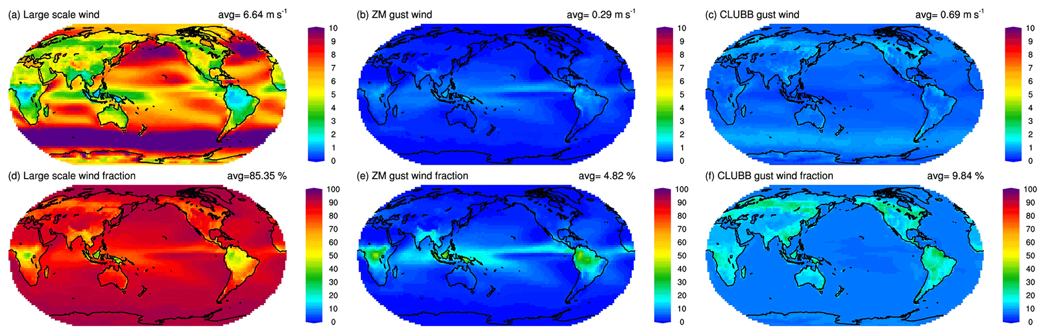
Figure 1Present-day EAMv1 climatology of wind speed (m s−1) at the lowest model level in (a) resolved motion, (b) gustiness associated with the ZM parameterization, and (c) gustiness associated with the CLUBB parameterization. Panels (d)–(f) are the fractional contribution of the three components to the total wind speed.
Next, we considered the subgrid temperature perturbation in the parcel buoyancy calculation in the ZM scheme. The subgrid temperature perturbation is set to 0.5 K in the Community Atmosphere Model version 5 (CAM5) (Neale et al., 2010) and 0.8 K in EAMv1 (Rasch et al., 2019). This treatment assumes that the subgrid heterogeneity of temperature is globally uniform. However, subgrid variability of temperature should vary in space and time. In particular, subgrid temperature heterogeneity is typically larger over land than over ocean. Setting a globally uniform subgrid temperature perturbation can potentially create biases in the distribution of deep convection. To address this deficiency, we computed the subgrid temperature perturbation by taking the square root of the subgrid temperature variance (a prognostic variable in CLUBB) and passed that information through ZM's parcel buoyancy calculation to account for the variability of the subgrid temperature perturbation. Based on sensitivity tests, a scaling factor of 2.0 was introduced to enhance the effect so that the simulated tropical clouds are in better agreement with observations (as discussed in Sect. 3).
Accounting for the gustiness effects and the variability of subgrid temperature variance was designed for EAMv1 running at ∼ 1∘ horizontal grid spacing. It is logical to expect that increasing model spatial resolution will reduce the impacts of these subgrid effects. Thus, a retuning of these subgrid effects would likely be needed when the model is run at a different horizontal resolution. The model configuration with only the gustiness effects and the subgrid temperature variance added to EAMv1 is labeled as EAMv1_SGV.
While EAMv1_SGV improves the spatial distribution of tropical clouds and precipitation (discussed in Sect. 3), tropical CREs and precipitation become overly strong after these changes, indicating a need for additional tuning to compensate for the unintended changes. Among all the tunable parameters, we targeted the ones that were heavily tuned in EAMv1 and adjusted their values to be closer to their theoretical or nominal values. For context, in EAMv1, the coefficients controlling the autoconversion rate in convective clouds c0_lnd and c0_ocn (which are inversely proportional to the timescale that condensate is converted to precipitation) were set to 0.007, more than 3 times larger than the nominal rate used in Lord et al. (1982). The consequence is that little condensate is detrained from convective updrafts, producing cirrus clouds with very low water content in the upper troposphere. To compensate for the weak source of ice water, EAMv1 assumes more Aitken mode sulfate aerosols are efficient homogeneous ice nuclei. As a result, EAMv1 produces relatively high cloud ice number (Ni) with small ice water content and weak sedimentation rates, making the cirrus clouds more persistent and highly reflective. In this recalibration, we chose to take the following steps:
-
increase the supply of condensed water to cirrus clouds by reducing c0_lnd and c0_ocn to their nominal value 0.002,
-
reduce the deep convective cloud fraction parameter dp1,
-
increase the downdraft mass fraction parameter alfa,
-
reduce the assumed ice crystal radius detrained from deep convection (ice_deep),
-
increase the sensitivity of deep convection to surface temperature changes by reducing the number of lowest layers skipped for computing maximum moist static energy (mx_bot_lyr_adj) (while maintaining numerical stability),
-
enhance the lateral entrainment of deep convection by increasing the magnitude of dmpdz.
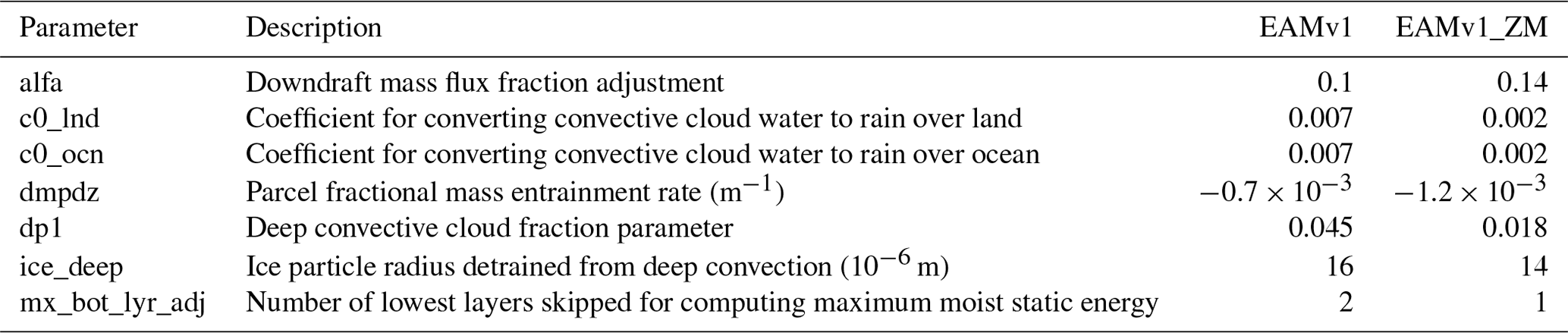
It is worth noting that changing dmpdz has different effects on CREs in different parts of the tropics and a significant impact on the subtropical CREs, but the exact mechanism is unclear and requires further investigation. We took an iterative approach to retune the model, adjusting one parameter at a time and assessing its impacts after each simulation. The model configuration with only these ZM parameter changes added to EAMv1 is labeled as EAMv1_ZM (Table 1).
Table 1Description of tunable parameters and their values in EAMv1 and EAMv1_ZM.
In addition to changes made to the deep convection scheme in EAMv1_ZM, we also introduced two microphysical changes in MG2 in order to refine the tropical CRE (Table 3): (1) we increased the size threshold for sulfate aerosols to act as homogeneous ice nuclei (so4_sz_thresh_icenuc) to reduce ice number concentration and increase ice crystal size and thus the sedimentation rate and (2) increased ice_sed_ai to further increase the ice sedimentation rate. Combining the two MG2 changes with EAMv1_SGV and EAMv1_ZM, these adjustments increase cloudiness in the western and eastern Pacific, decrease cloudiness in the central Pacific, and cause weaker subsidence in the subtropics.
2.2 Subtropical low clouds
Realistic simulation of low clouds across various cloud regimes requires not only a realistic simulation of the large-scale meteorological conditions but also a versatile parameterization that is able to describe different subgrid characteristics of clouds and atmospheric thermodynamic conditions in different cloud regimes. Following Medeiros and Stevens (2011), cloud regimes are determined by the vertical velocity at 500 hPa and the lower tropospheric stability. We also assessed the geographical distribution of those clouds. The CLUBB parameterization employed in EAMv1 uses a multivariate probability density function (PDF) to describe the subgrid variability of cloud, thermodynamic, and dynamic variables, all of which are closely connected to changes in the subgrid vertical velocity w′. The second and third moments of w′, and , are prognostic variables in CLUBB, meaning that the skewness of the w′ PDF, ), is predicted according to the governing equations. This is a critical treatment because it allows CLUBB to produce different subgrid characteristics in different regimes. As illustrated in Golaz et al. (2002), a low skewness corresponds to a rather symmetric PDF of w′ characteristic of the stratus and stratocumulus regimes, whereas a high skewness is more characteristic of a trade cumulus regime in which stronger and isolated updrafts embedded in subsidence occur more frequently. In principle, CLUBB can be used to represent the deep-convection regime as well (Thayer-Calder et al., 2015; Guo et al., 2015), but it requires significant amount of effort to enable said unification such that EAMv1 still uses ZM for a separate treatment of deep convection. The limit of Skw≤4.5 is imposed in EAMv1 in order to prevent numerical instability in CLUBB's equations. To simulate different subgrid variabilities in different regimes, CLUBB uses different damping coefficients and different widths of the w′ PDF as a function of Skw: for X* set to the diffusivity or variance of a CLUBB's prognostic variable (e.g., vertical velocity variance, total water variance), , where X* is a linear combination of low skewness values X (C1, C11, and gamma_coef in Table 2) and high skewness values Xb (C1b, C6rtb, C6rthlb, C11b, and gamma_coefb in Table 2) with a weighting factor , where Xc is a transition factor (C1c, C6rtc, C6rthlc, C11c, gamma_coefc in Table 2). For instance, the damping coefficient for , C1*, is expressed as a function of skewness, C1, C1b, and C1c: .
Table 2Description of tunable parameters and their values in EAMv1 and EAMv1_CLUBB.
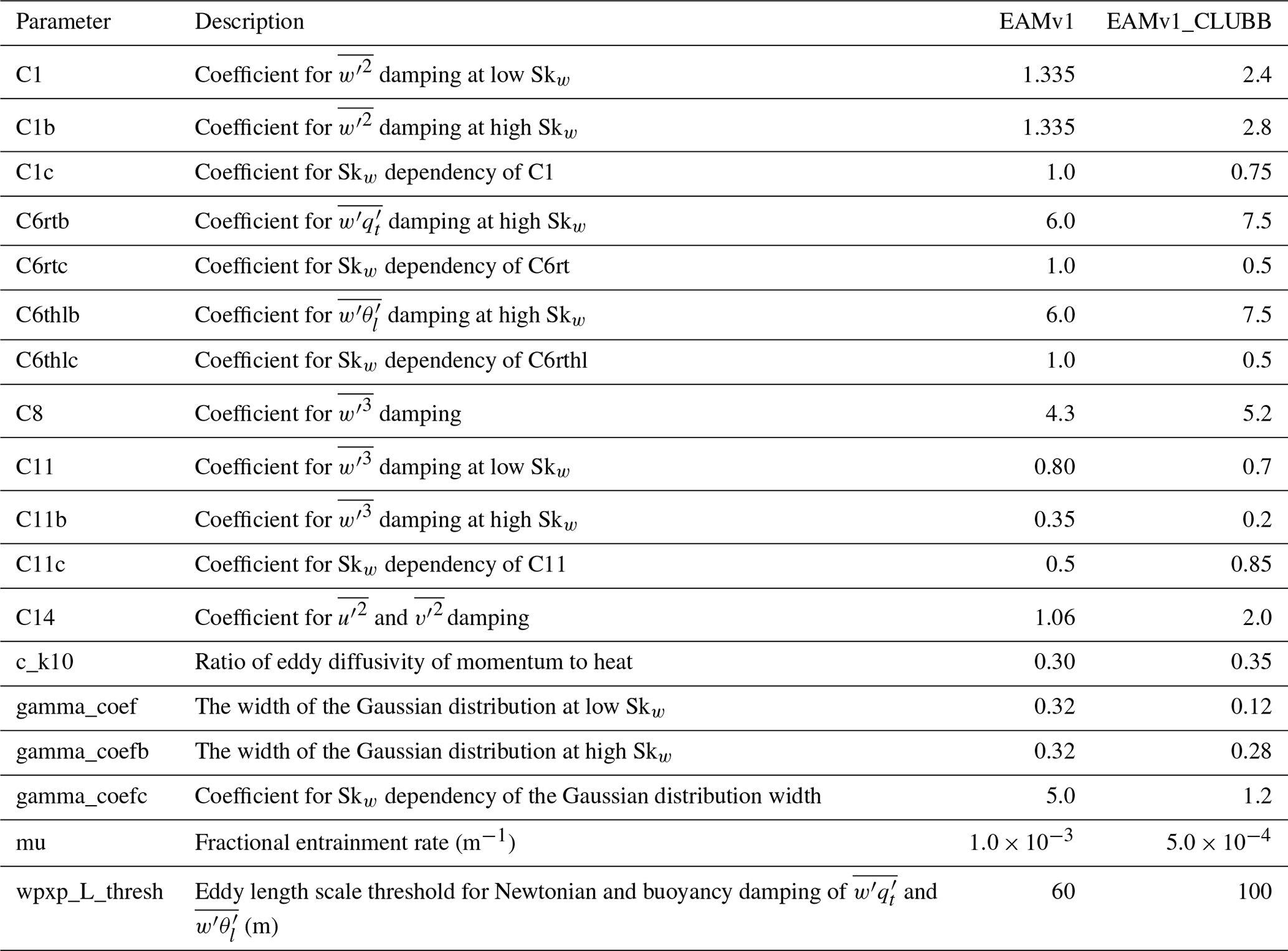
Although this variable skewness treatment provides a way to simulate different subgrid characteristics in different regimes, it is poorly constrained – the equation describing X* and the chosen values of parameters X, Xb, and Xc are somewhat ad hoc. In EAMv1, we set C1b and gamma_coefb to be the same as C1 and gamma_coef, respectively, to reduce unconstrained assumptions. This is a simple choice that reduces the number of free parameters in CLUBB, but it also limits the flexibility of the CLUBB parameterization with implications for the model fidelity. As shown in Brunke et al. (2019), EAMv1 produces overly bright shallow Cu and a significant bias in near-coast Sc. Therefore, we explored a different pathway in this study by setting C1 and C1b and gamma_coef and gamma_coefb to different values and used the simulated low-cloud CREs as the tuning target to determine the parameter values. Improvements in the simulated clouds are significant, as will be shown in Sect. 3. However, it is worth noting that these improvements do not suggest that this treatment or the parameter settings are the correct representation of the physical processes in the real world. Rather, our study should be viewed as a demonstration that it is useful to enable the variable skewness treatment to facilitate the production of different subgrid characteristics in different cloud regimes. Reducing the level of complexity of the physics may sometimes compromise the model fidelity and can lead to further uncertainties in climate projections. As we further show in Sect. 3, these changes also affect aerosol–cloud interactions, cloud feedbacks, and, ultimately, climate sensitivity. Future studies that employ sufficient observations (from Doppler lidar, for example) or large eddy simulations (LES) to either constrain the parameter values in the current parameterization or develop a new parameterization to mimic the real-world subgrid characteristics in different regimes would be highly valuable.
To recalibrate CLUBB, we first increased the overall cloudiness through the following processes.
-
We weakened the turbulent mixing in the planetary boundary layer (PBL), which reduces PBL decoupling and mixing between the PBL and the free troposphere. This was achieved by increasing C1, C1b, C6rtb, C6rthlb, and C14; increasing C_k10; and increasing the eddy length scale threshold (Fig. 2a, b).
-
We facilitated cloud formation by reducing the width of the w′ PDF via reducing gamma_coef and gamma_coefb.
-
We promoted Sc-like symmetric mixing rather than shallow Cu-like asymmetric mixing by reducing Skw via increasing C8.
-
We allowed larger horizontal variation in subgrid characteristics by enlarging the difference in parameter values between high- and low-skewness regimes (i.e., X's and Xb's), as determined from satellite observations (Z. B. Zhang et al., 2019), and modified the Xc values to refine the transition between low- and high-skewness regimes.
The change in the width of the w′ PDF also affects the in-cloud liquid water mixing ratio (Qc) variance, resulting in variable enhancement factors for warm rain processes in cloud microphysics. We also reduced the cloudiness in the shallow Cu regime by decreasing the lateral entrainment (i.e., reducing mu). These changes increase the skewness in the shallow Cu regime (Fig. 2c, d), and lead to a realistic Sc-to-Cu transition (as discussed in Sect. 3). The model configuration with only these CLUBB parameter changes added to EAMv1 is labeled as EAMv1_CLUBB (Table 2).
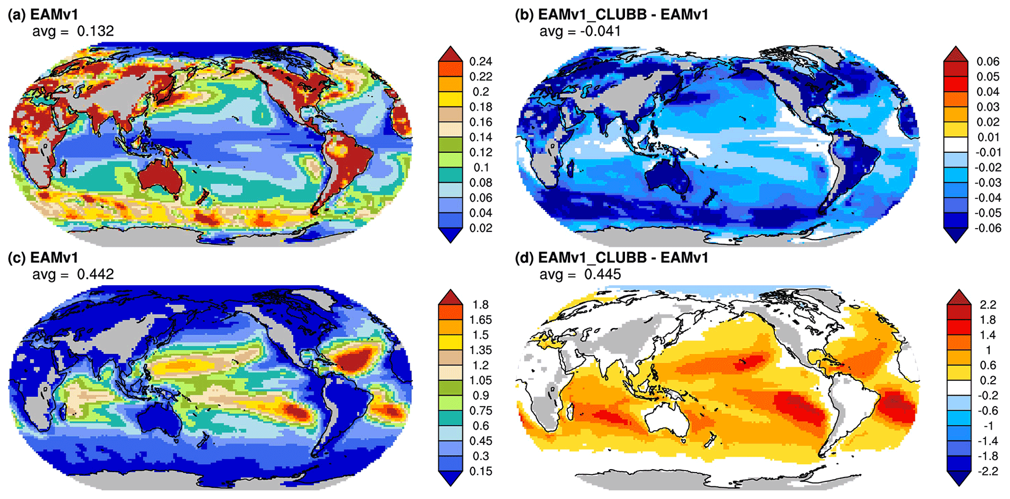
Figure 2Present-day climatology of (a) mean subgrid vertical velocity variance (; unit = m2 s−2) at 925 hPa in EAMv1. (b) The difference between EAMv1_CLUBB and EAMv1. (c) The skewness of subgrid vertical velocity () in EAMv1. (d) The Skw difference between EAMv1_CLUBB and EAMv1 at 925 hPa.
Uncertainties in cloud microphysical processes affect all non-deep convective clouds, including subtropical clouds. The tuning of the microphysical processes is justified by fundamental process-level uncertainties and simplifying assumptions made in bulk microphysics schemes (including the MG2 scheme used in EAMv1) regarding particle size distributions and the subgrid scale distribution of cloud properties. To increase cloudiness in the Sc regime, we weakened cloud-top entrainment by enhancing droplet sedimentation (Bretherton et al., 2007). Next, we reduced the lower bound of subgrid vertical velocity used for cloud droplet nucleation (wsubmin). This improves the coupling between the simulated subgrid updraft velocity and the cloud microphysical properties such as droplet number, size, and condensate amount. We also adjusted the warm rain processes by restoring the heavily tuned prc_exp1, the exponent of droplet number (Nc) in the autoconversion parameterization in EAMv1 (Rasch et al., 2019), to the nominal value based on observations (Wood, 2005). This increases cloudiness in areas where more aerosols are present. The accretion process is also enhanced to compensate for the reduction of precipitation from the change in autoconversion. The above microphysical modifications designed to optimize stratocumulus will be combined with additional microphysical tunings inspired by cloud types at other latitudes (see Sect. 2.3).
It is worth noting that the autoconversion parameterizations in EAMv1 is based on Khairoutdinov and Kogan (2000), which is a function of Qc and Nc. However, the parameter values (i.e., the scale factor and exponents of Qc and Nc) for different cloud regimes are very different (Kogan, 2013), indicating that the autoconversion process is governed by more factors than those considered in the current parameterization. Therefore, there is no one set of parameter values that can optimally represent the autoconversion process for all cloud regimes. Adjusting these parameters to achieve reasonably good representation of cloud and precipitation simulations is possible, but one should use caution when interpreting the results and acknowledge the fundamental deficiency of the underlying process representations in the model. Given the importance of warm rain processes (autoconversion and accretion) in simulating clouds and precipitation and their responses to forcings, developing new parameterizations that can flexibly represent these processes over a broad range of cloud types to address this model deficiency should be included in the roadmap toward next generation ESMs.
2.3 Midlatitude and high-latitude clouds
Another significant cloud bias present in midlatitude and high-latitudes in EAMv1 can be attributed to excessive supercooled liquid clouds due to a suppressed Wegener–Bergeron–Findeisen (WBF) process (Rasch et al., 2019). This insufficient conversion from liquid to ice is a consequence of an inherited value of a scaling factor of 0.1 that tuned down the WBF process rate significantly. The WBF rate was previously tuned down in order to address an underestimate supercooled liquid clouds in CAM5 (Tan et al., 2016; DeMott et al., 2010; Liu et al., 2011). However, EAMv1 eliminated one of the sources of this bias by replacing the Meyers et al. (1992) ice nucleation (IN) scheme from CAM5 with a classical nucleation theory (CNT)-based scheme (Hoose et al., 2010; Wang et al., 2014). The CNT scheme addresses the overproduction of ice crystals by Meyers et al. (1992), which scavenges liquid water rapidly. Replacing the Meyers et al. (1992) scheme but maintaining the slow WBF conversion from liquid to ice produced unrealistically high liquid water path (LWP) in midlatitudes and high latitudes: the LWP poleward of 60∘ N and over the Southern Ocean is 15 %–30 % higher than the LWP in the tropics (see discussion in Sect. 3.1; Fig. 3). Such an unrealistic meridional distribution of LWP can cause significant biases in the radiative energy distribution, atmospheric circulation, and water cycle. The excessive cloud liquid water in midlatitudes and high latitudes can also lead to strong aerosol–cloud interactions and biases in long-range transport of aerosols due to strong wet scavenging (Wang et al., 2013). The high-resolution configuration of E3SMv1 reverted the IN scheme to Meyers et al. (1992) to address this bias (Caldwell et al., 2019), but the error compensation from two incorrect cloud processes can potentially produce biases in cloud microphysical properties, adversely impacting the credibility of climate projections.
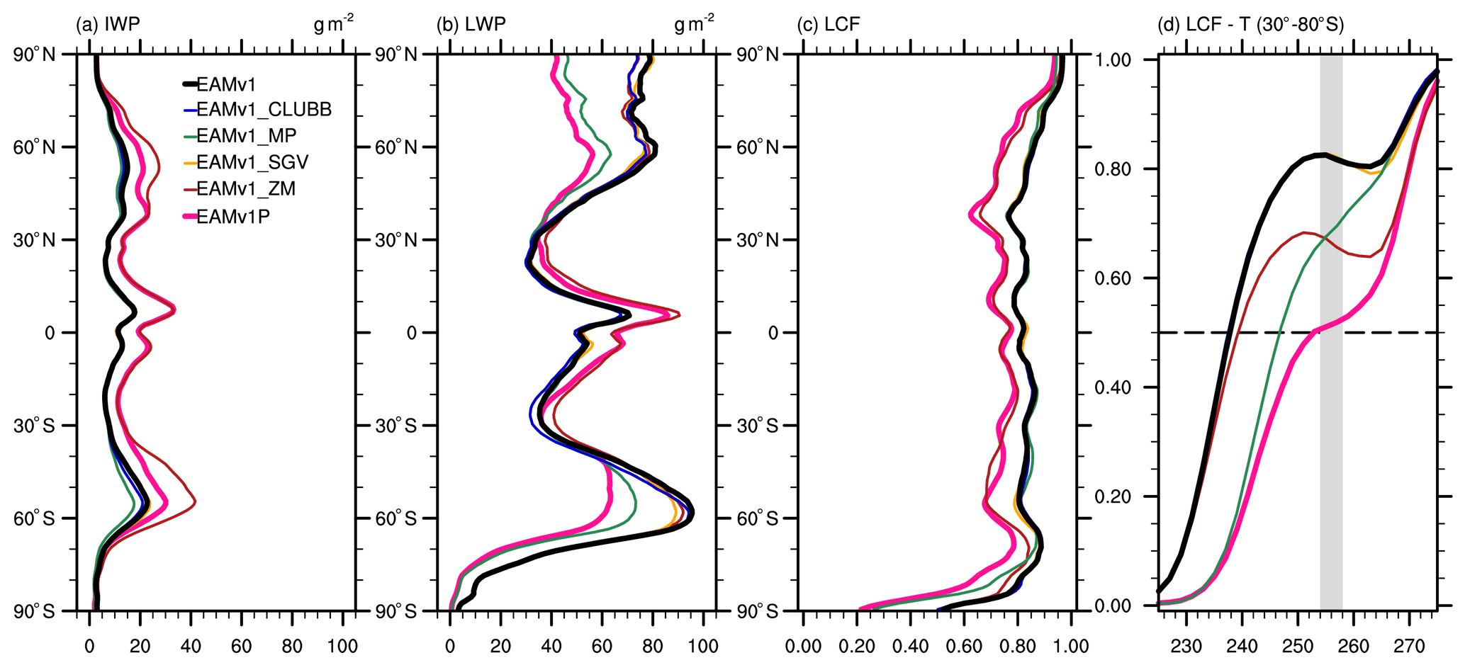
Figure 3Zonal mean of (a) ice water path (IWP), (b) liquid water path (LWP), and (c) liquid condensate fraction (LCF), defined as the ratio of liquid to total cloud condensate amount, and (d) LCF as a function of temperature (unit = K) between 30 and 80∘ S. The horizontal dashed line in (d) denotes T5050 (McCoy et al., 2016, 2015), where ice and liquid each contributes to 50 % of the total condensate. The observational estimate of T5050 range (McCoy et al., 2016) are shown in the gray-shaded area.
In this study, we adopted an alternative approach to address this bias. Y. Zhang et al. (2019) shows that improvements can be made by increasing the WBF process rate. Therefore, we retained the new CNT-based IN scheme that had been shown to perform better than the Meyers et al. (1992) scheme and significantly increased the scale factor for the WBF process to increase the conversion from liquid to ice. This adjustment is superposed with additional benefits from the parameter adjustments in the ZM scheme (Sect. 2.1) that improved the upper-tropospheric ice clouds in the tropics and increased ice clouds in the midlatitudes. The model configuration with only the MG2 parameter changes added to EAMv1 is labeled as EAMv1_MP (Table 3). The combination of EAMv1_MP and EAMv1_ZM lead to lower LWP and higher ice water path (IWP) in the midlatitudes and high latitudes (see discussion in Sect. 3.1; Fig. 3).
Table 3Description of tunable parameters and their values in EAMv1 and EAMv1_MP.

2.4 Model simulations
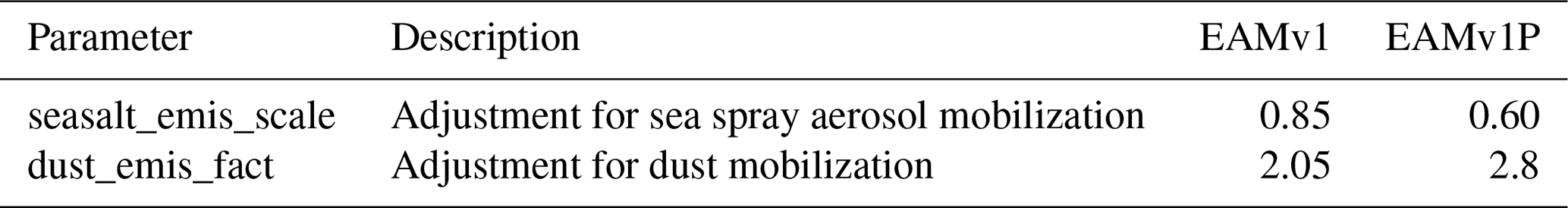
The final revised model (labeled as EAMv1P) includes all changes discussed above and two additional changes to the scale factors for emissions of sea spray and dust aerosols (Table 4) so that the global mean aerosol optical depth (τaer) is similar between EAMv1 and the recalibrated model.
Table 4Description of scale factors of emissions and their values in EAMv1 and EAMv1P.
In this paper, we show model results from grouped parameter adjustments instead of individual parameter changes. Model configurations are listed in Table 5. The effects and the mechanisms of each individual parameter adjustment require further investigation and will be documented in separate papers.

Each model configuration was used for 11-year global atmospheric simulations (the first year was discarded as spin-up) in which the atmosphere model was coupled with an interactive land model but sea surface temperature (SST) and sea ice cover were prescribed. Emissions of aerosols and their precursors were obtained from CMIP phase 6 (CMIP6) emission datasets (Hoesly et al., 2018; van Marle et al., 2017). We ran the coarse-resolution EAM configuration (i.e., ne30np4, which corresponds to approximately 1∘ horizontal grid spacing) with
-
present-day (here 2000 CE) forcing;
-
pre-industrial (here 1850 CE) forcing;
-
present-day forcing, except for pre-industrial aerosol emissions;
-
pre-industrial forcing with SST elevated by 4 K uniformly;
-
present-day forcing with SST, sea ice, and solar constant set to pre-industrial conditions.
We compute the effective radiative forcing (ERF) from these prescribed SST and sea ice experiments (Hansen et al., 2005). Forster et al. (2016) compared different methodologies for computing the ERF and recommend the prescribed SST and sea ice method. The differences between (1) and (3) provide information on the impacts of anthropogenic aerosols. Contrasting (2) and (4) provides climate feedback estimates. Total anthropogenic ERF (ERFant), also termed total adjusted forcing, is derived by comparing (5) and (2) (Forster et al., 2013). ERFant includes anthropogenic forcing (greenhouse gas concentrations, aerosols, and land use land cover change) and rapid adjustments in water vapor, clouds, and temperature.
3.1 Clouds
Table 6 summarizes the global mean present-day climatology of cloud properties using the various model configurations listed in Table 5. Satellite observations summarized in Stubenrauch et al. (2013) and Neubauer et al. (2019) are also provided, but we note that it is dangerous (and can be misleading) to compare model state variables with satellite retrievals without using a simulator since large retrieval and sampling uncertainties exist. The CREs are computed by double radiation calls in the model. Shortwave and longwave CREs contributed from liquid clouds, ice clouds, convective clouds, and snow are independently computed. Rain droplets are not radiatively active in EAMv1. Because radiative transfer is nonlinear, the sum of the CREs from clouds and snow are not equal to the total CRE.
Table 6Global mean 10-year-averaged cloud properties of EAMv1, EAMv1_CLUBB, EAMv1_MP, EAMv1_SGV, EAMv1_ZM, EAMv1P, and satellite observations summarized in Stubenrauch et al. (2013) and Neubauer et al. (2019). Relevant cloud properties listed here are TOA shortwave cloud radiative effects (SWCRE; unit = W m−2) and those of liquid clouds (SWCREliq), ice clouds (SWCREice), snow (SWCREsnow), and convective clouds (SWCREconv); TOA longwave cloud radiative effects (LWCRE; unit = W m−2) and those of liquid clouds (LWCREliq), ice clouds (LWCREice), snow (LWCREsnow), and convective clouds (LWCREconv); cloud fraction (unit = %) of the total column (Fcld,tot), below 700 hPa (Fcld,low), between 400 and 700 hPa (Fcld,med), and above 400 hPa (Fcld,hgh); optical depth of all clouds (τcld) and that of liquid clouds (τliq), ice clouds (τice), snow (τsnow), convective clouds (τconv), and all clouds below 700 hPa (τlow) and above 400 hPa (τhgh); column-integrated total LWP (unit = g m−2) and IWP (unit = g m−2), Nc (unit = 109 m−2) and Ni (unit = 109 m−2); altitude of the top (Zhgh,top; unit = km) and base (Zhgh,top; unit = km) of clouds above 400 hPa; and altitude of the top (Zlow,top; unit = km) and base (Zlow,top; unit = km) of clouds below 700 hPa.
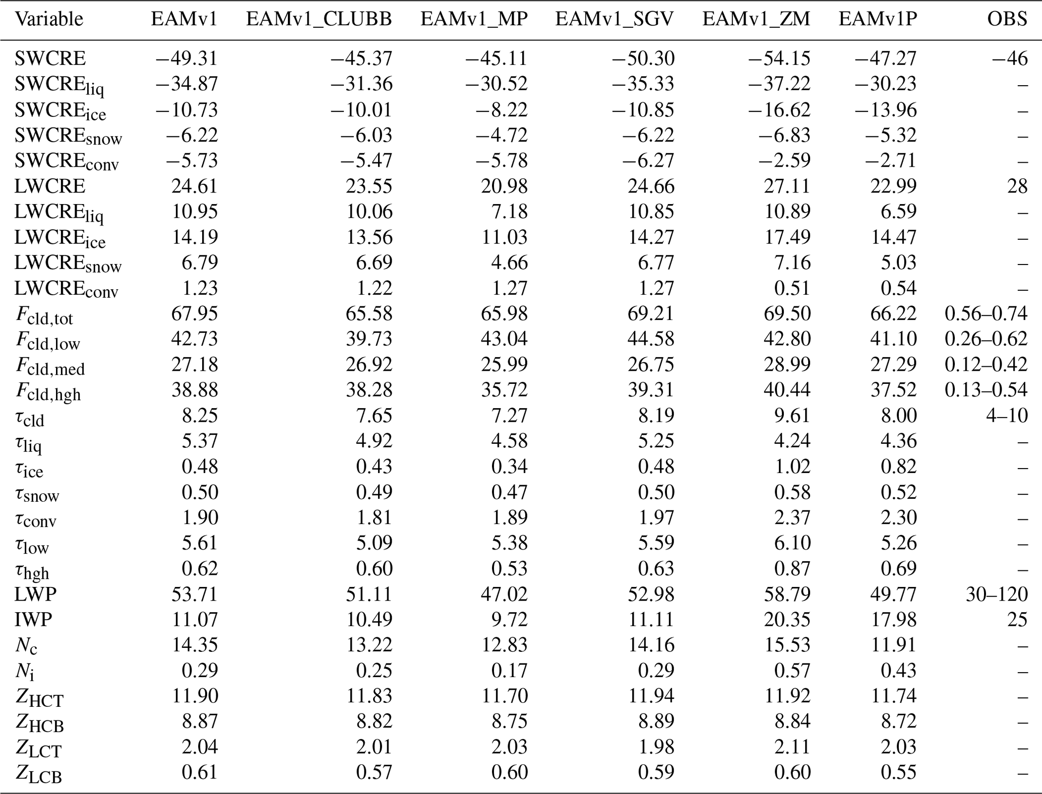
Compared with EAMv1, EAMv1_CLUBB shows lower-magnitude top-of-atmosphere (TOA) net CREs due primarily to a reduction of liquid clouds in the shallow Cu regime. EAMv1_MP also produces lower-magnitude total shortwave and longwave CREs, but it is attributable to the reduction of CREs from both liquid and ice clouds from increasing the WBF process. EAMv1_SGV only marginally increases CREs, but EAMv1_ZM significantly enhances the CREs from liquid and ice clouds, though the convective CREs are significantly reduced in EAMv1_ZM because the convective cloud fraction is much lower as a result of reducing the deep convective cloud fraction parameter dp1. The CRE differences are consistent with the differences in cloud optical depth (τcld). In contrast, cloud fractions and cloud heights are relatively invariant between different configurations. EAMv1_MP reduces LWP, IWP, Nc, and Ni mostly at midlatitudes and high latitudes, and EAMv1_ZM increases them mostly in the tropics. The EAMv1P configuration combines all of the changes and produces global mean net CRE (−24.28 W m−2) not very different from that in EAMv1 (−24.7 W m−2), but we emphasize that the spatial distribution of clouds is as important as global mean values because different cloud regimes may respond to perturbations differently.
Figure 3 shows that the changes made in EAMv1_ZM increase the IWP significantly at most latitudes except the polar regions. This is likely due to the combination of reducing the convective autoconversion efficiency (by reducing c0_lnd and c0_ocn) and decreasing the ice particle size detrained from deep convection (by reducing ice_deep), which increases the ice crystal number and prolongs the lifetime of ice clouds. EAMv1_MP shows a slight reduction of IWP in the Southern Ocean, while significantly reducing LWP in midlatitudes and high latitudes. This remedies the unrealistically high LWP in those regions in EAMv1 due to its weak WBF process.
These changes in condensate also lead to a more realistic liquid condensate fraction (LCF) thermal dependence (Fig. 3d). Because of the general IWP increase in EAMv1_ZM, the meridional distribution of LCF is reduced as a result of changes made in ZM (Fig. 3c). Interestingly, the global mean atmospheric temperature where ice and liquid each contribute to 50 % of total condensate, T5050 (McCoy et al., 2015, 2016), in EAMv1 is about 240 K, which is significantly lower than observational estimates of 254–258 K (McCoy et al., 2016). While the CMIP5 models tend to freeze liquid condensates at higher temperatures (Cesana et al., 2015; Tan et al., 2016; McCoy et al., 2016), EAMv1 appears to have overcorrected this bias and produced excessive supercooled liquid at low temperatures. Consistent with Y. Zhang et al. (2019), EAMv1_MP increases the T5050. Combining with changes introduced in EAMv1_ZM, EAMv1P produces a much more reasonable T5050 of 254 K, which is at the lower bound of the observational estimates. We note that even though Hu et al. (2010) provided an observationally derived LCF–T relationship based on the Cloud–Aerosol Lidar and Infrared Pathfinder Satellite Observation (CALIPSO) measurements (Winker et al., 2007), EAMv1 does not have the CALIPSO cloud-phase simulator (Cesana and Chepfer, 2013), and thus a fair comparison is not possible. Evaluating the model LCF–T relationship against satellite observations in a consistent way will be very useful and requires further investigation.
Differences in the simulated cloud phase can have important implications for aerosol–cloud interactions (ACI) because the physical processes regulating the interactions between aerosols and warm cloud and between aerosols and cold clouds are very different. The simulated cloud phase can also affect cloud feedbacks to warming (Tan et al., 2016). The ACI and cloud feedbacks will be discussed in Sect. 3.4 and 3.5.
Figure 4 illustrates how the most challenging TOA shortwave cloud radiative effect (SWCRE) biases in EAMv1 (Fig. 4a) are greatly remedied by the cumulative effects of our retuning (Fig. 4f), with intermediate subpanels decomposing the grouped parameter changes in ways that help illustrate how they are intended to address those biases independently and jointly. By enabling the variable skewness treatment in CLUBB and the adjustments that follow, the overly bright shallow Cu and the significant lack of Sc in EAMv1 are greatly improved in EAMv1_CLUBB. SWCRE associated with coastal Sc is increased by about 10–20 W m−2 off the coast of California and by about 30–40 W m−2 off the coast of Peru and Chile, while over the shallow Cu regime SWCRE is reduced by 20–30 W m−2. The elevated Skw in the shallow Cu regime also reduces the cloud water removal timescale (not shown). In EAMv1_MP, tuning up the WBF process corrects the SWCRE bias at midlatitudes and high latitudes. With increasing fraction of ice condensate, the cloud water removal timescale is reduced (not shown) because warm rain processes are less efficient in removing condensate than ice precipitation processes (Mülmenstädt et al., 2021). Adjustments to cloud droplet sedimentation and warm rain processes make moderate improvements to Sc. Changes to ice crystal sedimentation and sulfate aerosol size result in significant reduction in tropical SWCRE, as upper tropospheric clouds respond to these adjustments the most. Furthermore, EAMv1_SGV increases clouds in areas where large-scale winds are weak and convection occurs frequently, including the TWP and Amazonia. Some effects on the eastern Pacific are also observed. EAMv1_ZM further increases cloudiness in the ITCZ, especially in the western and eastern Pacific. Cloudiness in the Southern Pacific Convergence Zone (SPCZ) is also improved. Setting c0_lnd and c0_ocn to lower values essentially slows down the convective autoconversion process, leading to longer water removal timescales in the tropics. Combining all the changes, EAMv1P shows improved cloud distribution with reduced biases in the tropics, subtropics, midlatitudes, and high latitudes, indicating that the changes discussed in Sect. 2 are appropriate.
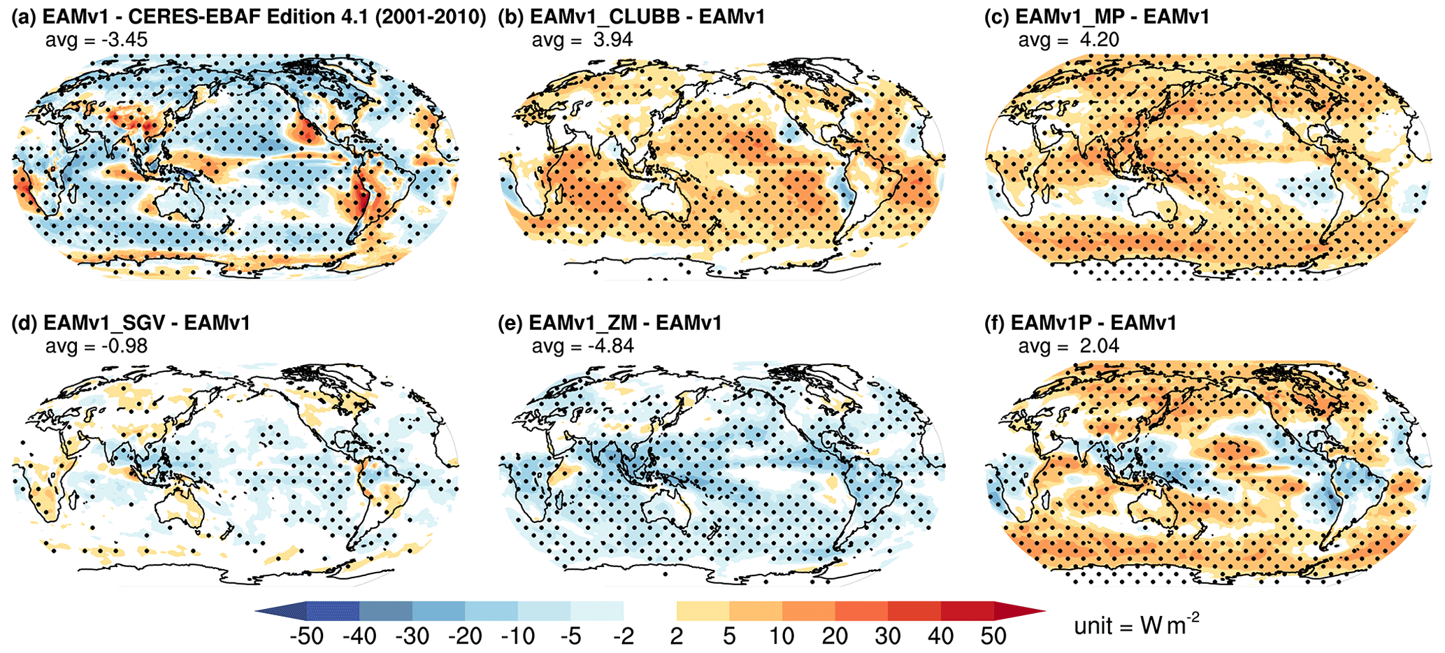
Figure 4Difference in present-day TOA SWCRE (W m−2) climatology between (a) EAMv1 and Clouds and Earth's Radiant Energy System (CERES) (Wielicki et al., 1996) Energy Balance and Filled (EBAF) Edition 4.1 (Loeb et al., 2012, 2003, 2018) averaged over 2001–2010, (b) EAMv1_CLUBB and EAMv1, (c) EAMv1_MP and EAMv1, (d) EAMv1_SGV and EAMv1, (e) EAMv1_ZM and EAMv1, and (f) EAMv1P and EAMv1. Model TOA SWCRE values are 10-year averages. Stippling denotes significant difference at the 95 % confidence level based on a Student's t test.
Further evaluation using the Cloud–Aerosol Lidar and Infrared Pathfinder Satellite Observation (CALIPSO) cloud simulator (Chepfer et al., 2008), as part of the Cloud Feedback Model Intercomparison Project (CFMIP) Observation Simulator Package (COSP) (Bodas-Salcedo et al., 2011), that samples the model at 13:30 local time (LT) for comparisons of total cloud fraction with version 3.1.2 of the General Circulation Model-Oriented CALIPSO Cloud Product (GOCCP) (Chepfer et al., 2010) shows similar results. Figure 5 shows cloud bias reductions in the Northern Hemisphere high latitudes, the stratocumulus regions, the TWP, and over tropical lands. These improvements match our expectations, increasing our confidence in the model clouds. However, there are some differences between the comparisons in Figs. 4 and 5. In Fig. 4, EAMv1 shows overly bright clouds in trade cumulus regions and over the Southern Ocean, and EAMv1P reduces these biases. Figure 5 shows that EAMv1 produces less clouds in trade cumulus regions and more clouds over then Southern Ocean than GOCCP, and EAMv1P increases the bias in trade cumulus regions and does not change the Southern Ocean bias. This could indicate that the improvements to the TOA SWCRE over these regions are achieved by compensating errors between cloud fraction and cloud optical depth.
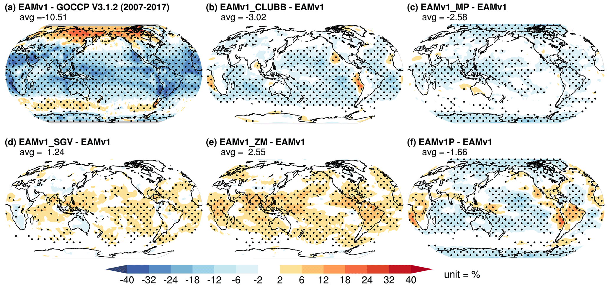
Figure 5Total cloud fraction between (a) EAMv1 and the version 3.1.2 of the GOCCP total cloud fraction (Chepfer et al., 2010) averaged over 2007–2017, (b) EAMv1_CLUBB and EAMv1, (c) EAMv1_MP and EAMv1, (d) EAMv1_SGV and EAMv1, (e) EAMv1_ZM and EAMv1, and (f) EAMv1P and EAMv1. Model cloud fractions are derived from the CALIPSO cloud simulator (Chepfer et al., 2008) sampled at 13:30 LT.
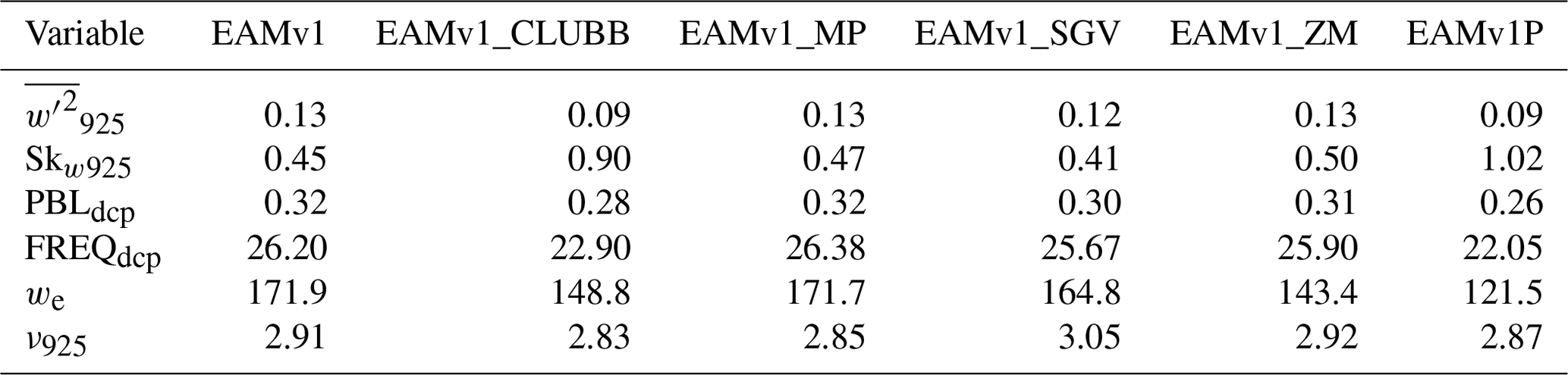
Given the importance of low clouds in Earth's radiation budget, we investigate the planetary boundary layer (PBL) properties in different model configurations to gain insights into the physical mechanisms associated with the parameter adjustments. Table 7 shows that the adjustments to CLUBB parameters affect the simulated PBL properties significantly (as expected). The adjustments to CLUBB parameters directly reduce the and increase Skw925, but they also govern the turbulent mixing and cloud processes in the PBL, producing a complex set of overall impacts on the macroscale properties of the PBL. The weaker indicates a shallower PBL, reducing both the PBL decoupling strength (PBLdcp), defined as the difference between cloud base height and lifting condensation level (LCL) (Jones et al., 2011), and the frequency of occurrence of decoupled PBL. The cloud-top entrainment rate for PBL clouds (we) is reduced as a result. It is interesting to note that the changes to the ZM deep-convection scheme can also reduce cloud-top entrainment, presumably through strengthening of the large-scale subsidence in the subtropics. On the other hand, higher Skw925 indicates that the model produces more asymmetric mixing and shallow Cu-like clouds. This matters for cloud feedback since an increase in Cu-like clouds and decrease in Sc-like clouds can lead to weaker low-cloud feedback (Cesana et al., 2019), and results will be discussed further in Sect. 3.5. Finally, we find that the inverse relative variance of cloud water, which affects the enhancement factors of autoconversion, accretion, and immersion freezing (Morrison and Gettelman, 2008), are not sensitive to the parameter changes. Thus, there is a limited impact on these three processes from changes in subgrid in-cloud water variance.
Table 7Global mean 10-year-averaged PBL properties of EAMv1, EAMv1_CLUBB, EAMv1_MP, EAMv1_SGV, EAMv1_ZM, and EAMv1P. Relevant PBL properties listed here are subgrid vertical velocity variance (, unit = m2 s−2) and the subgrid vertical velocity skewness (Skw) at 925 hPa, PBL decoupling strength (PBLdcp; unit = km), PBL decoupling frequency (FREQdcp; unit = %), cloud-top entrainment rate (we; unit = m d−1), and inverse relative variance of cloud water at 925 hPa (ν925). Only columns with clouds in PBL are sampled.
Next, we compare the estimated inversion strength (EIS) (Wood and Bretherton, 2006) between model simulations and a reanalysis dataset. The EIS was computed following the CFMIP diagnostics code catalogue (Tsushima et al., 2017). EIS has traditionally been considered as an important cloud-controlling factor affecting low clouds and low-cloud feedback (Klein et al., 2017; Myers et al., 2021). Figure 6 shows that EAMv1 generally underestimates EIS, except in the tropics. The revised model EAMv1P alleviates many of the biases, but some biases remain. EAMv1_CLUBB reduces the bias over land in general (except for in northern Africa) as well as the midlatitude and high-latitude ocean. EAMv1_MP shows significant difference in the polar regions, indicating that reducing supercooled liquid in the mixed-phase cloud regime can change polar PBL properties. EAMv1_SGV enhances the EIS as a result of convection invigoration. Similarly, EAMv1_ZM directly reduces the bias in the tropics and produces enhanced EIS in midlatitudes and high latitudes through large-scale circulation responses.
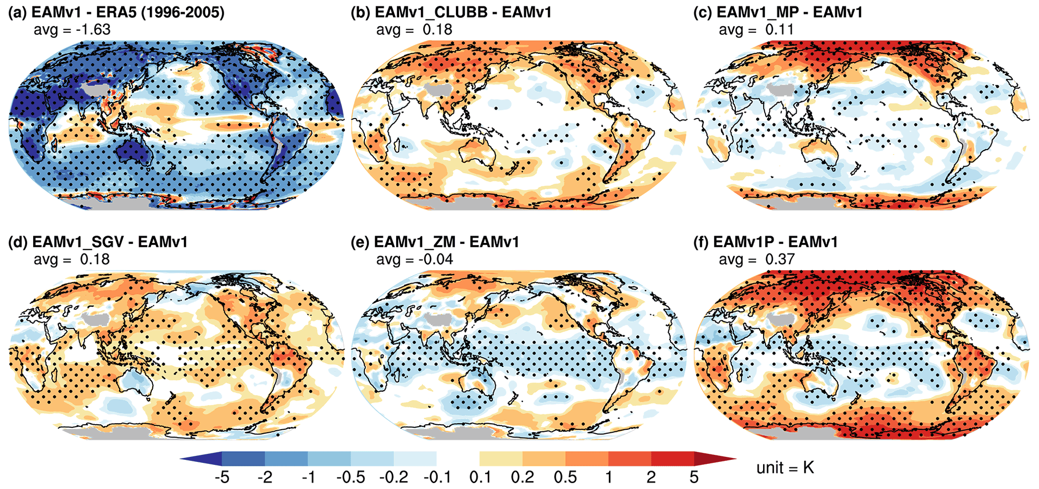
Figure 6Estimated inversion strength (EIS; unit = K). The EIS computed from the European Centre for Medium-Range Weather Forecasts' (ECMWF's) fifth-generation global meteorological reanalysis (ERA5) (Hersbach et al., 2019a) is used for the comparison with EAMv1.
Figure 7 shows that changes in EAMv1_CLUBB also significantly reduce the PBL decoupling strength (Jones et al., 2011). The decoupled PBL is often a sign that the PBL grows too deep, and thus the negative buoyancy at the top of the PBL is insufficient to mix through the sub-cloud layer (Wood, 2012). These conditions favor the transition from Sc to shallow Cu (Wood, 2012; Xiao et al., 2011), reducing the overall cloudiness and contributing to the lack of Sc in EAMv1. This long-standing regional cloud bias is primarily alleviated by adjustments to CLUBB parameters, particularly the increases in C1 and C1b that reduce . Furthermore, EAMv1_SGV also reduces the PBL decoupling strength over tropical land and subtropical and midlatitude ocean, likely due to the enhanced surface flux that moistens the PBL. The recalibrated model EAMv1P shows the collective effect of significant reduction in decoupling strength (Fig. 7) and frequency (not shown).

Figure 7PBL decoupling strength (unit = m) defined as the difference between LCL and the altitude of the cloud base (Jones et al., 2011). The PBL decoupling strength is computed at every cloud physics time step (dt=5 min), averaged over samples where decoupled PBL is detected.
We also diagnose the cloud-top entrainment efficiency (Bretherton et al., 2007) in different model configurations to further clarify the physical mechanisms associated with the parameter adjustments. Cloud-top entrainment efficiency is defined as , where we is the entrainment rate computed by differencing the resolved vertical motion and change in inversion height (zi), Δb is the virtual potential temperature jump scaled into buoyancy jump (), where the reference virtual potential temperature θref is 300 K, and w* is the convective velocity () that measures the buoyancy integrated over the boundary layer, where b′ is the buoyancy perturbation and is the buoyancy flux. Figure 8 shows that the largest differences are again a result of changes made in CLUBB. As is reduced, EAMv1_CLUBB produces a shallower PBL consistent with a reduced cloud-top entrainment efficiency. In EAMv1_MP, the enhancement of liquid and ice sedimentation also reduces entrainment efficiency (Bretherton et al., 2007). EAMv1_SGV generally enhances the surface fluxes and produces a deeper and relatively less stable PBL, leading to enhanced mixing between the PBL and the free troposphere.
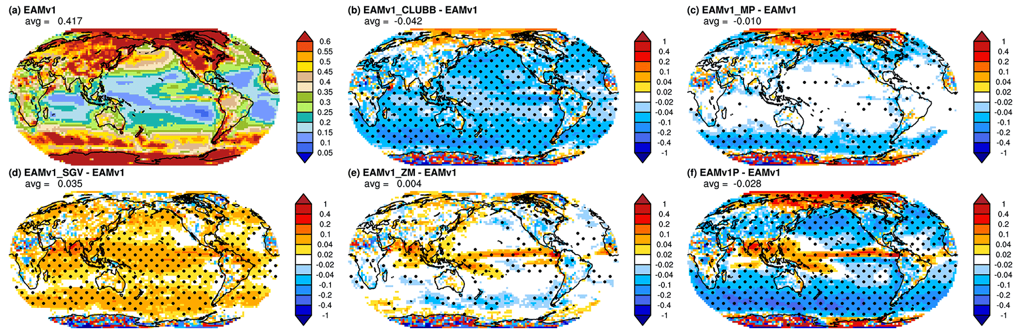
Figure 8Cloud-top entrainment efficiency (Bretherton et al., 2007). The cloud-top entrainment efficiency is computed at every cloud physics time step (dt=5 min) of the model.
The changes in PBL decoupling strength and cloud-top entrainment efficiency shown in Figs. 7 and 8 are consistent with expectations and affirm our understanding of the physical mechanisms connecting the parameter adjustments, CREs, and PBL properties, even though they are not directly controlled by any tunable parameters. Unfortunately, currently there is no global observational estimate for decoupling frequency and cloud-top entrainment efficiency, and thus we cannot assert that the recalibration improves these physical mechanisms when taken alone. However, put together they constitute a reassuring sign that relevant metrics of macroscale low-cloud dynamics are associated with desired changes in TOA SWCRE in logical ways. Future studies that derive decoupling frequency and cloud-top entrainment efficiency, as well as other important cloud-controlling factors, from field campaign measurements for evaluating models in particular regions and time periods would be highly valuable.
3.2 Precipitation
Table 8 shows the global mean precipitation characteristics. We find that adjustments to the ZM scheme (e.g., reducing the convective autoconversion efficiency and convective cloud fraction) lead to a reduction of convective precipitation (PRECC) and an increase in large-scale precipitation (PRECL). Here convective precipitation refers to the precipitation produced by the ZM deep-convection parameterization and large-scale precipitation refers to the precipitation produced by the MG2 cloud microphysics parameterization. While EAMv1 produces more convective precipitation than large-scale precipitation, the revised model EAMv1P corrects this bias so that the model is in better agreement with observational estimates (Yang et al., 2013). The shift from convective to large-scale precipitation is expected to improve precipitation characteristics (Yang et al., 2013) because more detailed cloud microphysics processes are considered for large-scale clouds.
Table 8Global mean 10-year-averaged precipitation fields of EAMv1, EAMv1_CLUBB, EAMv1_MP, EAMv1_SGV, EAMv1_ZM, and EAMv1P. Relevant precipitation variables listed here are total, convective, and large-scale precipitation rates (PRECT, PRECC, and PRECL, respectively; unit = mm d−1); ratio of deep convective precipitation to total precipitation (Rconv); frequency of occurrence (unit = %) of no precipitation (FREQdry), drizzle with precipitation rates less than 0.5 mm d−1 (FREQdrizzle), light precipitation with precipitation rates between 0.5 and 8 mm d−1 (FREQlight), moderate precipitation with precipitation rates between 8 and 80 mm d−1 (FREQmoderate), and heavy precipitation with precipitation rates exceeding 80 mm d−1 (FREQheavy); and ratio of autoconversion to total precipitation (Rauto).
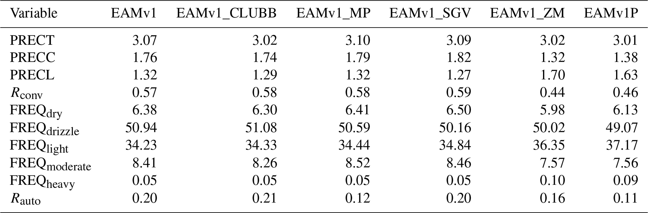
Nevertheless, the common bias in ESMs of producing frequent drizzle and light precipitation is pronounced in EAMv1, and adjustments of parameters have only a marginal impact. This suggests that the precipitation PDF bias is not related to parametric uncertainty and perhaps is attributed to model's structural deficiency such as issues with the trigger and closure in its deep-convection scheme or the coarse resolution, which is insufficient to simulate strong moisture convergence or dependency of precipitation formation on unresolved mesoscale forcing. Such an interpretation is consistent with many intercomparisons between super-parameterized and conventionally parameterized versions of the Community Earth System Model (CESM) (Kooperman et al., 2016) that have sampled different structural formulations for rainfall production. Recent studies indicated that using an improved convective trigger (Xie et al., 2019) or incorporating a stochastic convection scheme (Wang et al., 2021) into ZM can also help address the “too-frequent–too-weak” precipitation biases in EAMv1. Lastly, we show that the fraction of large-scale precipitation produced by autoconversion (Rauto in Table 8) in EAMv1 is already much lower than its predecessor model CAM5 even at 0.25∘ horizontal grid spacing (Ma et al., 2015), and the changes in EAMv1_MP further reduce the autoconversion fraction. This change will affect the model estimate of aerosol indirect effects (Posselt and Lohmann, 2009; Wang et al., 2012; Gettelman et al., 2013).
As discussed in Rasch et al. (2019) and shown in Fig. 9, EAMv1 produces high annual mean precipitation over the globe, over high elevations, over the Maritime Continent, and in the central Pacific but low annual mean precipitation over Amazonia and the oceanic TWP. With an improved cloud distribution, we find the precipitation simulation improves as well. Figure 9 shows that tropical precipitation is greatly improved. EAMv1_SGV enhances precipitation in the TWP, eastern Pacific, and Amazonia, whereas EAMv1_CLUBB and EAMv1_ZM reduce precipitation in the central Pacific and western Indian Ocean while increasing precipitation in the SPCZ. This suggests that the displaced Walker circulation in EAMv1 is significantly improved in the recalibrated model. EAMv1_SGV also reduces precipitation bias over high-elevation regions such as the Andes and Himalayas (likely through non-local circulation response). We also find an unexpected improvement from the ZM changes by reducing the double ITCZ bias. While the physical mechanism remains unclear and requires further investigation, our results corroborate the finding of Song and Zhang (2018) that the double ITCZ bias is sensitive to the adjustments in the deep-convection parameterization, which affects the tropical clouds (and energy budget) and precipitation directly and the large-scale circulations indirectly.

Figure 9Total precipitation rate differences (unit = mm d−1). The Global Precipitation Climatology Project (GPCP) version 2.3 dataset (Huffman et al., 2001; Adler et al., 2018) is used for the comparison with EAMv1.
In summary, the recalibrated model with improved clouds also produces more realistic present-day precipitation climatology. Pronounced precipitation biases in the tropics, over land, and over high elevations are significantly reduced. The improved realism of the precipitation distribution is consistent with the improved cloud distribution. These improvements lead to a more realistic atmospheric circulation and positive impacts on other aspects of the simulated atmosphere. The remaining biases in tropical clouds and precipitation could be related to the coarse model resolution, which fails to resolve islands, narrow mountain ranges, mesoscale convection, and small-scale meteorological fields (Wang et al., 2018), and also has a deficiency in representing the triggering of deep convection (Xie et al., 2019). The lack of representing ice clouds in CLUBB can also contribute to remaining biases in midlatitudes and high latitudes (Zhang et al., 2020).
3.3 Other aspects of the present-day climate
Our recalibration is governed by an understanding of the physical mechanisms present in the atmosphere and their representation in parameterizations. Our effort has focused on improving the CREs across cloud regimes. Improvements to clouds and precipitation have been accomplished that are consistent with our expectations, but an evaluation of other aspects of the simulated present-day climate is essential. While the possibility of compensating biases always exists, our confidence in the underlying physics in the model will be increased if many other aspects are also improved. Otherwise, we are forced to suspect that the model achieves its behavior primarily through compensating biases.
Near-surface air temperature is an important state variable for validating the fidelity of the ESMs. Both dynamical and physical processes affect the temperature field, and thus an appropriate balance between these processes is essential for producing a realistic simulation of present-day conditions. Therefore, the near-surface air temperature can also be viewed as a minimum requirement for providing some confidence in projections of future climate. However, like many weather and climate models (Morcrette et al., 2018), EAMv1 produces significant near-surface air temperature biases. The Northern Hemisphere (NH) high latitudes exhibit a 1–5 K warm bias, and there are cold biases in other places (Fig. 10). The warm high-latitude bias and the cold tropical bias produce a weaker Equator-to-pole temperature gradient, which can cause errors in midlatitude baroclinicity, storm tracks, and large-scale circulations. It can also lead to excessive melting of sea ice and land ice, which has adverse impacts on ocean circulation. Figure 10 shows that the parameter adjustments that aim to improve CREs generally improve the near-surface temperature, and the changes in EAMv1_MP lead to the largest improvements. This suggests that the liquid cloud bias in EAMv1 due to the underactive WBF process, coupled with the CNT-based IN parameterization, may be responsible for the near-surface temperature bias. Strong liquid-to-ice conversion improves the CREs and subsequently affects the near-surface temperature, which will further impact circulations and affect other aspects of the Earth's climate.
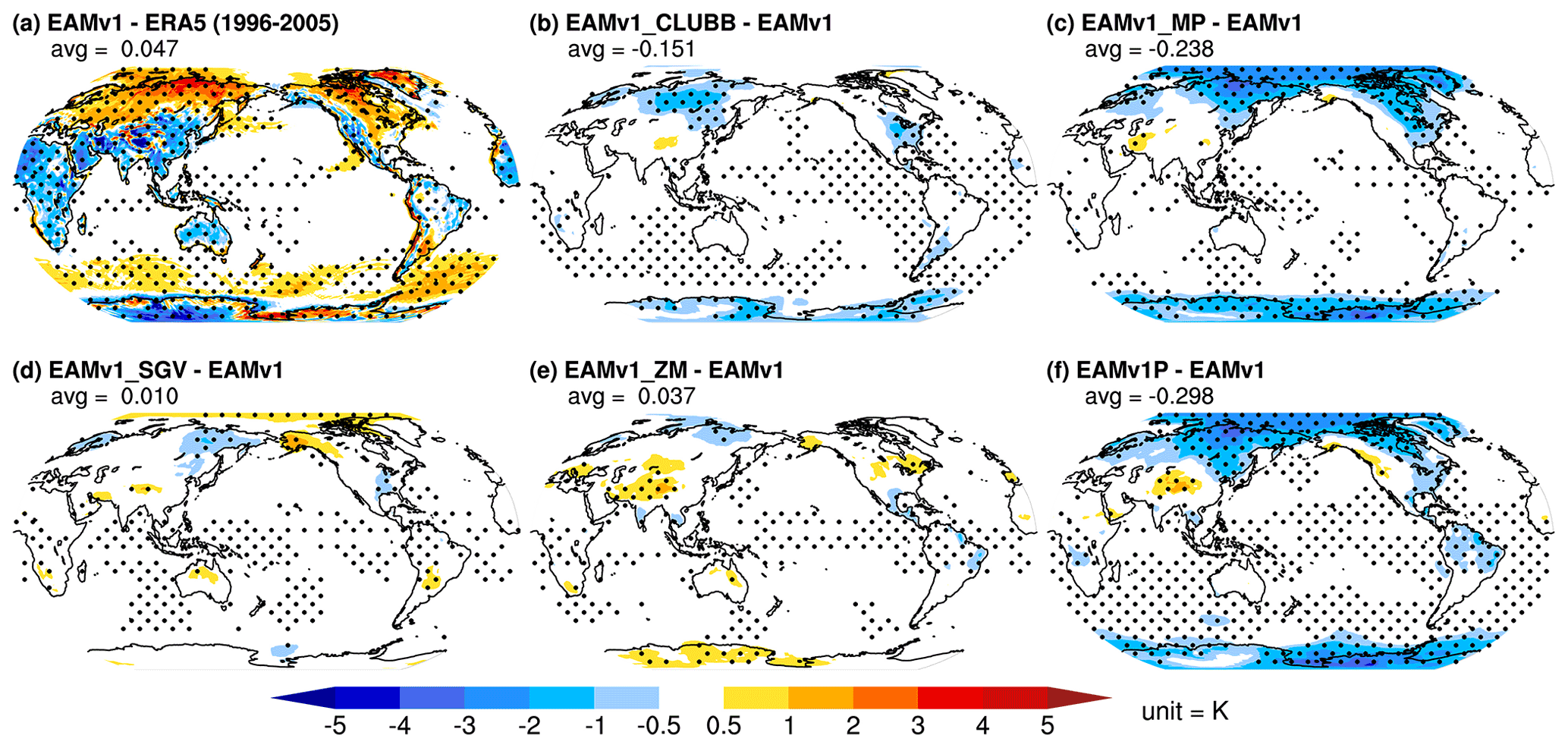
Figure 10The 2 m height air temperature (unit = K). The ERA5 reanalysis is used for the comparison with EAMv1.
Surface winds affect the physical climate and the biogeochemical cycle in a variety of ways. In EAMv1, surface winds affect surface flux of heat, moisture, and momentum, which influence the thermodynamic properties in the PBL but also more generally affect atmospheric energy and water cycles. The emissions of sea spray aerosols and mineral dust are a function of surface winds. Over the ocean, surface winds drive the ocean surface currents and influence the mixed-layer depth, heat budget, and carbon uptake in the ocean. Figure 11 shows that surface winds in EAMv1 are significantly stronger than those in the MERRA-2 reanalysis, especially in the Southern Ocean and North Atlantic. In the tropical Pacific Ocean, the trade easterlies are too strong, which pushes the cold tongue into the Indo-Pacific warm pool. The wind direction biases are reduced in EAMv1_SGV when the gustiness parameterization is enabled, such that the subgrid winds are accounted for in surface flux calculations. EAMv1_ZM also shows some minor improvements in TWP. Combining all the model changes, the revised model EAMv1P shows significant improvements in surface winds in many parts of the tropics, North Atlantic, and Southern Ocean. In the fully coupled E3SM, these improvements may lead to more realistic ocean circulations as well as ocean–atmosphere exchange of heat, moisture, momentum, trace gases, and aerosols.
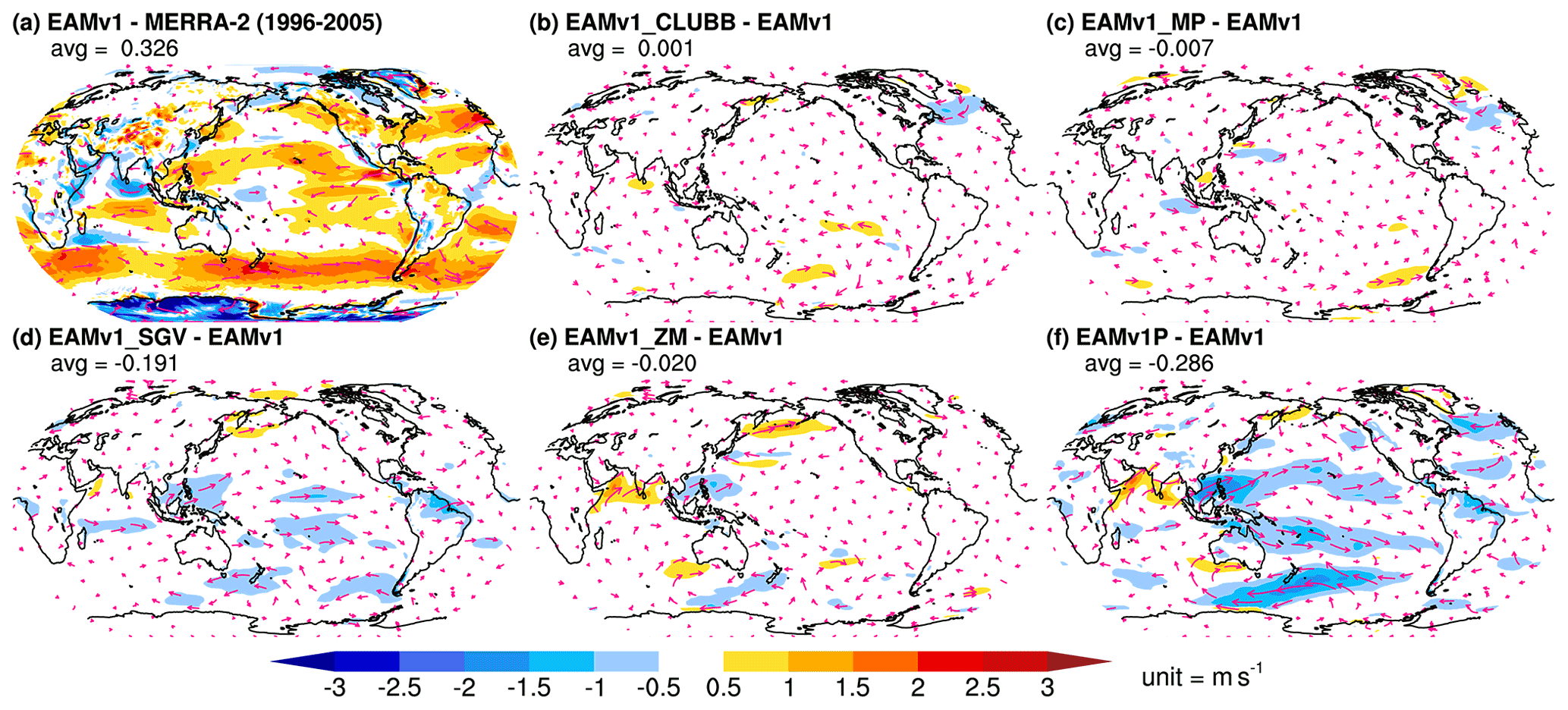
Figure 11Winds at the lowest model level. The surface winds from the Modern-Era Retrospective Analysis for Research and Applications Version 2 (MERRA-2) (Gelaro et al., 2017) is used for the comparison with EAMv1.
Although our recalibration is only targeted to improve CRE features (Fig. 4), those changes can affect aerosols as well because cloud processing is an important sink in the aerosol life cycle. Figure 12 shows that the changes in EAMv1_MP and EAMv1_ZM increase the aerosol loading, while EAMv1_SGV produces lower aerosol loading. The changes in aerosol loading are partially due to the changes in wet scavenging. In EAMv1_MP, the reduction of supercooled liquid water path increases aerosol loading in midlatitudes and high latitudes because liquid clouds remove aerosols efficiently. EAMv1_SGV enhances the surface moisture flux, which also increases wet scavenging, and the weakened convective autoconversion in EAMv1_ZM reduces the wet removal of aerosols. We also find that the revisions have reduced dust emissions over the Sahara because of the weakened turbulence in EAMv1_CLUBB. Collectively, the recalibrated model EAMv1P reduces the aerosol optical depth (τaer) biases in the NH midlatitudes and high latitudes, in the tropics, and over land in general. There are, however, remaining τaer biases in the subtropics, eastern Pacific, eastern Atlantic, and Southern Ocean.
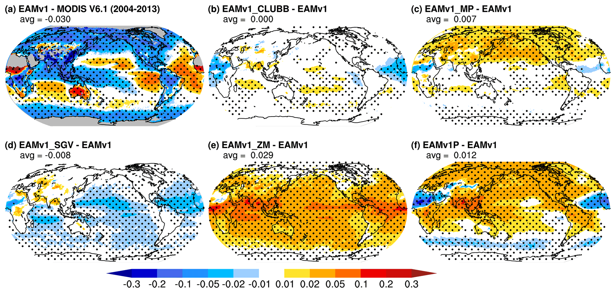
Figure 12Clear-sky aerosol optical depth (τaer). The MODIS onboard Aqua τaer data product (Levy et al., 2013) is used for comparison with EAMv1. Model clear-sky τaer is sampled at 13:30 LT.
In addition to improvements in near-surface temperature, surface winds, and column-integrated aerosols, we observe improvements to sea level pressure (SLP) and temperature and wind fields in the recalibrated model EAMv1P (Fig. 13). While EAMv1_CLUBB and EAMv1_MP do not produce different results from EAMv1, we find that the meridional wind at 850 and 500 hPa (coded as numbers 4 and 7) in EAMv1_SGV and EAMv1_ZM are in better agreement with ERA5 as their normalized standard deviation reduces. Many other aspects of the climate are carefully evaluated using E3SM standard diagnostics (https://portal.nersc.gov/project/e3sm/beharrop/EAMv1P/, last access: 14 February 2022). We find that the recalibrated model shows improvements in most aspects of the simulated present-day climate (despite the fact that they were not tuning targets), and low or no degradation in others. We conclude that when improvements in simulating clouds across regimes are achieved by applying adjustments based on an understanding of the physical mechanisms, those changes are manifested by more realistic simulation of many features of the global atmosphere. Because the correct response of the nonlinear climate system depends on both realistic base state and realistic process representations, the improved realism in the recalibrated model EAMv1P provides greater confidence in estimating the responses of the climate system to anthropogenic forcings and ultimately the ECS.
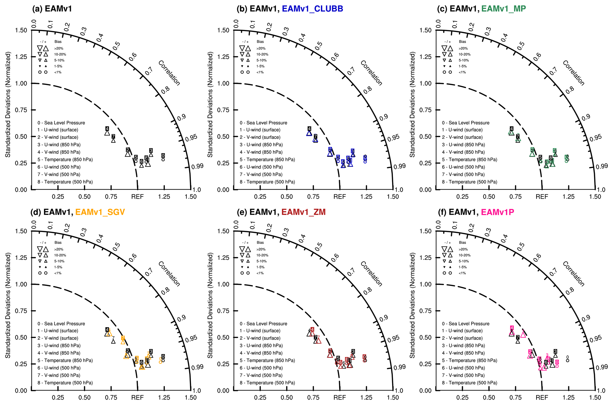
Figure 13Taylor diagram (Taylor, 2001) comparing sea level pressure, temperature, and winds in EAMv1, EAMv1_CLUBB, EAMv1_MP, EAMv1_SGV, EAMv1_ZM, and EAMv1P with the ERA5 reanalysis.
3.4 Responses to anthropogenic aerosols
The role of aerosols in the climate system is a major uncertainty in projections of Earth's future climate and in interpreting how the climate has been forced over recent decades. The uncertainty has been attributed to both a lack of understanding of aerosol emissions in pre-industrial times (Carslaw et al., 2013) and uncertainties associated with modeling aerosol and cloud processes (Regayre et al., 2018; Yoshioka et al., 2019). E3SMv1 produces notable biases in the historical evolution of surface temperature due to a combination of high ECS (from cloud feedback) and strong aerosol forcing, both of which are likely to be too large (Golaz et al., 2019). In this section, we assess the cloud and precipitation responses to anthropogenic aerosols in the recalibrated model where processes influencing aerosols and clouds operate differently from EAMv1 and the simulated present-day atmosphere is more realistic than that in EAMv1. Our goal is to understand the impacts and the physical mechanisms of the parameter adjustments on cloud and precipitation responses to aerosols. The effects of anthropogenic aerosols are assessed by differencing paired simulations where one uses the present-day aerosol emissions and the other uses the pre-industrial aerosol emissions (see Sect. 2 for the experiment design).
Table 9 shows the global mean net total ERFant in EAMv1 is quite low compared to CMIP5 (Forster et al., 2013) and other previous-generation models (Kiehl, 2007). This is mostly attributed to the aerosol ERF (ERFaer) (Golaz et al., 2019). EAMv1_MP increases ERFant, but other parameter adjustments lower ERFant so that the recalibrated model EAMv1P produces about the same ERFant. ERFaer comprises the ERF associated with aerosol–radiation interactions (ERFari), aerosol–cloud interaction (ERFaci), and aerosol-induced surface albedo changes. The ERFaer is computed by differencing all-sky TOA radiative flux between paired fixed SST simulations with present-day and pre-industrial aerosol emissions (Hansen et al., 2005), which is referred to as ERF_fSST in Forster et al. (2016). ERFaci is defined as the clean-sky TOA CRE difference (Ghan, 2013). Note that the Ghan (2013) method removes the direct radiative effect from the anthropogenic aerosols on CREs, producing stronger ERFaci (−1.48 W m−2) compared to the Boucher et al. (2013) method (∼ −1 W m−2) used in Wang et al. (2020), which assumes that ERFaci is the residual between ERFari+aci and ERFari. EAMv1 produces slightly weaker net ERFaer (−1.42 W m−2) and ERFaci (−1.48 W m−2) than its predecessor CAM5's −1.47 and −1.53 W m−2, respectively (Ghan et al., 2012). EAMv1's ERFaer falls within the 68 % confidence range of −1.6 to −0.6 W m−2 (where the 90 % confidence range is between −2.0 and −0.4 W m−2) estimated recently by considering various lines of evidence including models, observations, theories, energy balance requirements, and observed temperature constraints (Bellouin et al., 2020).
Table 9Global mean 10-year-averaged total ERFant derived from paired simulations with present-day and pre-industrial forcings. Shortwave, longwave, and net ERFaer; shortwave, longwave, net ERFaci (unit = W m−2); and the difference in total precipitation rate (PRECT, unit = mm d−1), land surface temperature (Ts; unit = K), and aerosol optical depth (τaer) difference between paired simulations with present-day and pre-industrial aerosol emissions are also given.
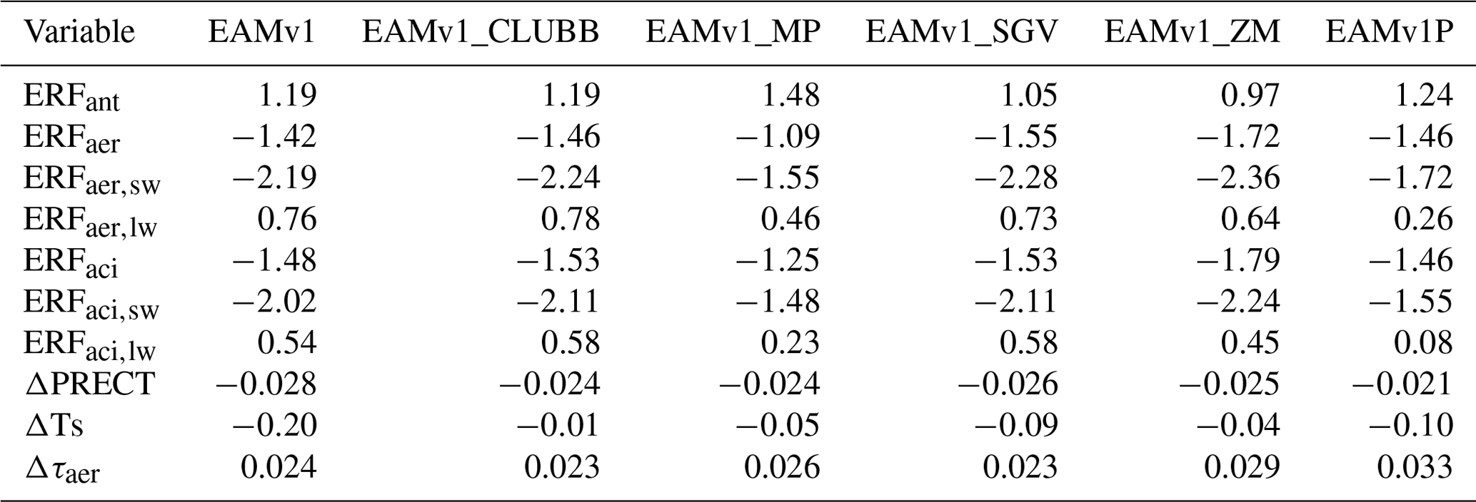
Collectively, the net ERFaci and ERFaer in EAMv1P remain about the same as EAMv1, but EAMv1P produces significantly weaker ERFaci,sw and ERFaci,lw. These are due to competing effects of our microphysical versus deep convective recalibrations. Our microphysical tunings in EAMv1_MP significantly weaken ERFaci for two reasons. First, EAMv1_MP reduces supercooled liquid clouds in the NH storm track from tuning up the WBF process, which weakens the ERFaci due to aerosol effects on liquid clouds. Second, EAMv1_MP reduces the sulfate aerosols participating in homogeneous ice nucleation, an expected consequence of having increased the size threshold of sulfate aerosols. Since ERFaci is mostly attributed to aerosol effects on liquid clouds in EAMv1, reducing the amount of baseline liquid clouds reduces ERFaci. Conversely, our tunings of the deep-convection scheme in EAMv1_ZM enhance ERFaci. Since the ZM scheme does not consider detailed cloud microphysical processes, this enhancement is likely due to the overall increase in cloudiness as shown in Fig. 1. Collectively, the net ERFaci and ERFaer in EAMv1P remain about the same as EAMv1, but EAMv1P produces significantly weaker ERFaci,sw and ERFaci,lw.
Both longwave and shortwave radiation affect surface temperature and atmospheric cooling rates, which govern the hydrological cycle. Because ERFaer is reduced for both shortwave and longwave in EAMv1P, the recalibrated model shows reduced aerosol-induced response in precipitation (Table 9) and land surface temperature (Table 9), even though the net ERFaer is about the same. Furthermore, the τaer difference between the paired simulations with present-day and pre-industrial aerosol emissions (Δτaer) in EAMv1P agrees much better with estimates from model ensembles (Watson-Parris et al., 2020) and from an estimate based on a combination of models and observations (Kinne et al., 2006) than that in EAMv1. Because Δτaer is significantly larger in EAMv1P than EAMv1, whereas ERFaci values in the two model configurations are similar, the sensitivity of CREs to aerosol perturbations (i.e., the change in CRE per unit aerosol perturbation) is lower in EAMv1P.
Figure 14 shows that the recalibration leads to a smaller magnitude of both positive and negative ERFaci in most places. The aerosol-induced strong warming in the Arctic and strong cooling in the NH storm track, East Asia, and North America are reduced, indicating a weaker local CRE response to aerosols in EAMv1P. EAMv1_MP again produces the most significant reduction, which we attribute to the more effective WBF process that reduces the supercooled liquid clouds. Other changes introduced in EAMv1_MP may also contribute to the weaker ERFaci in East Asia, the Northeast Pacific, and North America, including (1) enhancing the sedimentation of ice and liquid cloud droplets, (2) reducing the sulfate aerosols available for homogeneous ice nucleation, and (3) reducing the minimum subgrid vertical velocity used for liquid droplet nucleation. Regional exceptions with enhanced ERFaci magnitude also occur and are noteworthy in the subtropical stratocumulus regions off the Peruvian and Namibian coasts, where our recalibration has increased the amount of low cloud available to participate in aerosol-induced brightening.
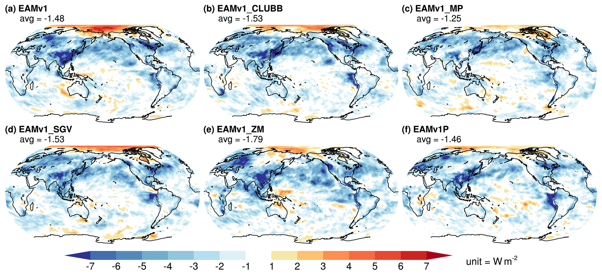
Figure 14ERFaci estimated using the Ghan (2013) method in (a) EAMv1, (b) EAMv1_CLUBB, (c) EAMv1_MP, (d) EAMv1_SGC, (e) EAMv1_ZM, and (f) EAMv1P.
Of particular note regarding model calibration against historical temperature changes are the response of aerosol-induced land surface temperature changes. In Fig. 15, we show that the strong influence of aerosols on surface temperature in EAMv1 is encouragingly reduced by each of our incremental recalibrations. Despite the fact that the global mean ERFaer remains the same in EAMv1P, the temperature effects are muted. With the reduced sensitivity of surface temperature to aerosol perturbations, we speculate that these recalibrations might ameliorate the concerning signature of the unrealistically strong cooling in the 1950s in E3SMv1 (Golaz et al., 2019) if the cause of the bias is indeed due to the overly strong aerosol forcing as hypothesized. We also find that aerosols induce opposite land temperature changes over northeastern Eurasia and northwestern North America. This indicates that the surface temperature changes are not determined only by local energy balance. Other processes in the climate system, such as large-scale circulation changes also play a role. Furthermore, an empirical relation has been shown to exist between the global mean ERFant and ECS in climate models from both the CMIP3 and CMIP5 collections (Kiehl, 2007; Forster et al., 2013). The relationship between ERFant and ECS exists because both values in models are sensitive to simulated clouds. Our tuning strategy specifically targets improving the representation of clouds, and it is worth asking whether these improvements uphold or alter the ERFant–ECS relation. The small difference in ERFant between the EAMv1 and EAMv1P configurations suggests the possibility of a similar small difference in ECS between these two configurations, and yet we find this is not the case (see Sect. 3.5).
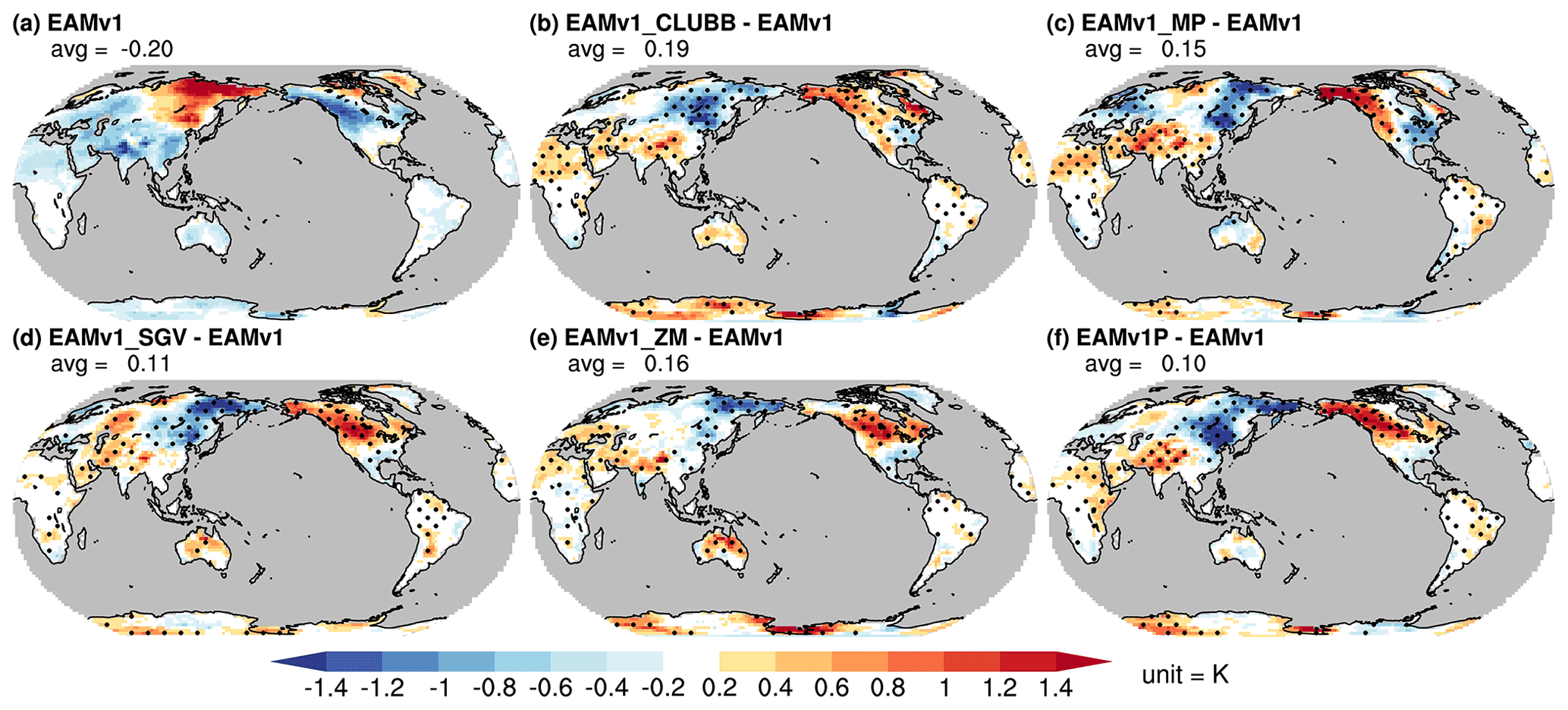
Figure 15Aerosol-induced changes in land surface temperature.
Table 10 shows that the aerosol-induced change in cloud fraction remains small in all model configurations. For column-integrated condensate amount, consistent with muted cloud radiative responses to aerosol, EAMv1_MP significantly reduces the sensitivity of LWP and IWP to aerosols. EAMv1_ZM also reduces the IWP sensitivity. The droplet and ice number concentrations are highly sensitive to anthropogenic aerosols as expected, but EAMv1_MP significantly reduces the sensitivity of both Nc and Ni to aerosols, while EAMv1_ZM only reduces the sensitivity of Ni to aerosol perturbations. By combining the present-day Nc and Ni in Table 6 and the relative change in Nc and Ni due to anthropogenic aerosols in Table 10, we find that EAMv1_ZM produces higher Nc and Ni in the unperturbed pre-industrial environment than those in EAMv1. EAMv1_ZM also produces a larger Nc increase (4.79 × 10⁹ m−2) due to anthropogenic aerosols than EAMv1 (4.58 × 10⁹ m−2), which is consistent with the larger ERFaci. Changes in cloud macrophysical and microphysical properties drive cloud optical property and radiative effect changes as well. EAMv1_MP reduces the sensitivity of τliq, τice, and τsnow to aerosols, leading to lower sensitivity of CRE for corresponding hydrometeors to aerosol perturbations. EAMv1_ZM also reduces the sensitivity of τice and τsnow to aerosols and the corresponding CRE sensitivities. This is likely due to the reduction of the ice particle size detrained from deep convection, which increases Ni in the unperturbed pre-industrial environment so that the ice clouds are less susceptible to aerosols. Finally, the revised model EAMv1P shows decreases in shortwave and longwave CRE responses.
Table 10The same as Table 6 but instead showing the change in cloud properties induced by anthropogenic aerosols relative to their pre-industrial values (unit = %). Variables are defined in Table 6.
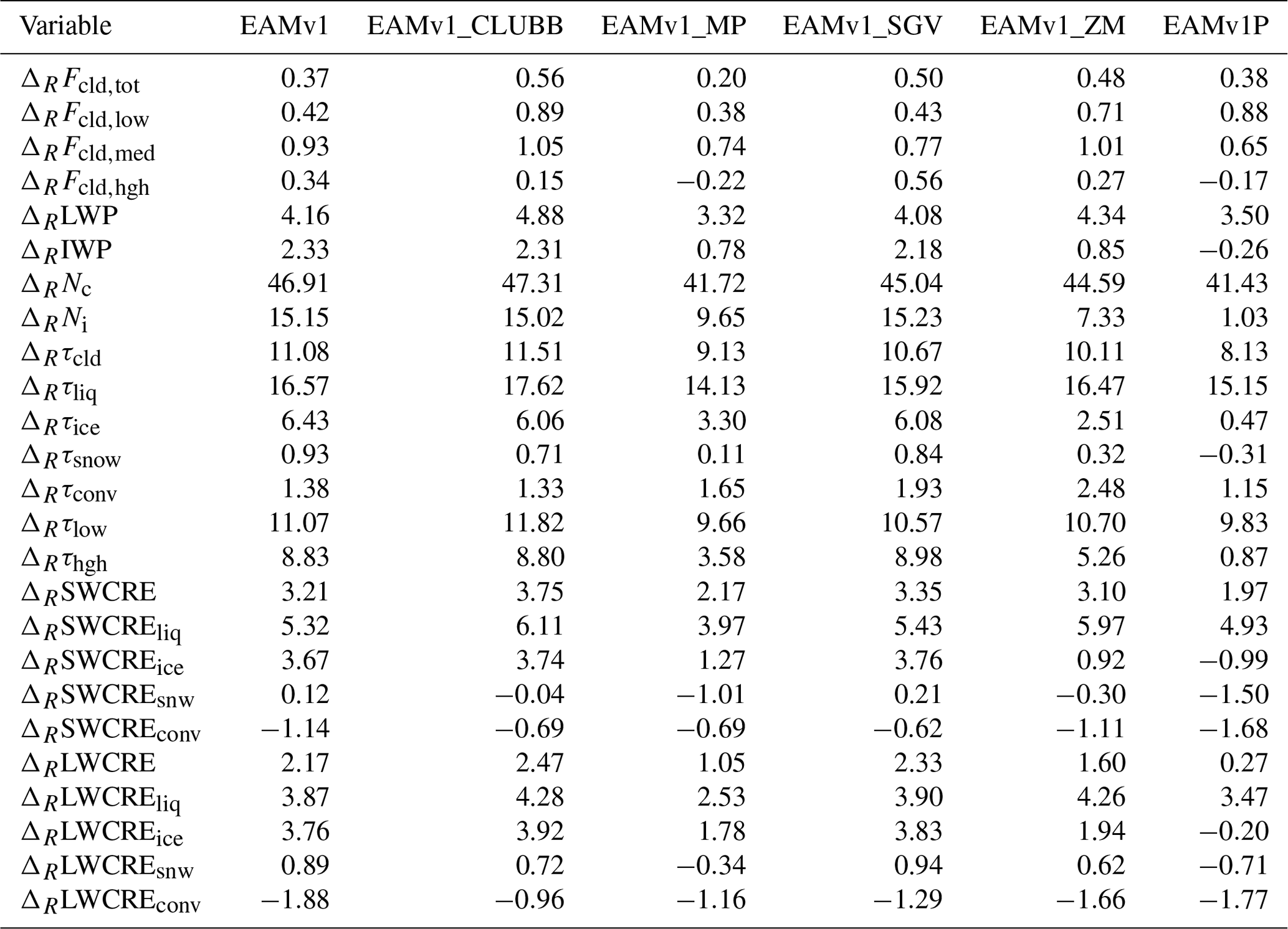
In addition to damping condensate and radiative responses to aerosol loading, our recalibration also reduces the sensitivity of precipitation intensity statistics. In EAMv1, anthropogenic aerosols reduce the frequency of occurrence of light precipitation (<2 mm d−1) across all large-scale dynamical regimes based on large-scale vertical velocity at 500 hPa, reduce light-to-moderate precipitation (<80 mm d−1) in strong ascending regions (<−20 hPa d−1), and increase precipitation between 2.5 and 20 mm d−1 in general (Fig. 16). The parameter adjustments in EAMv1_MP, EAMv1_SGV, and EAMv1_ZM all lead to weakened precipitation response compared to EAMv1. As a consequence, cloud and precipitation processes become less sensitive to aerosol perturbations in the recalibrated model.
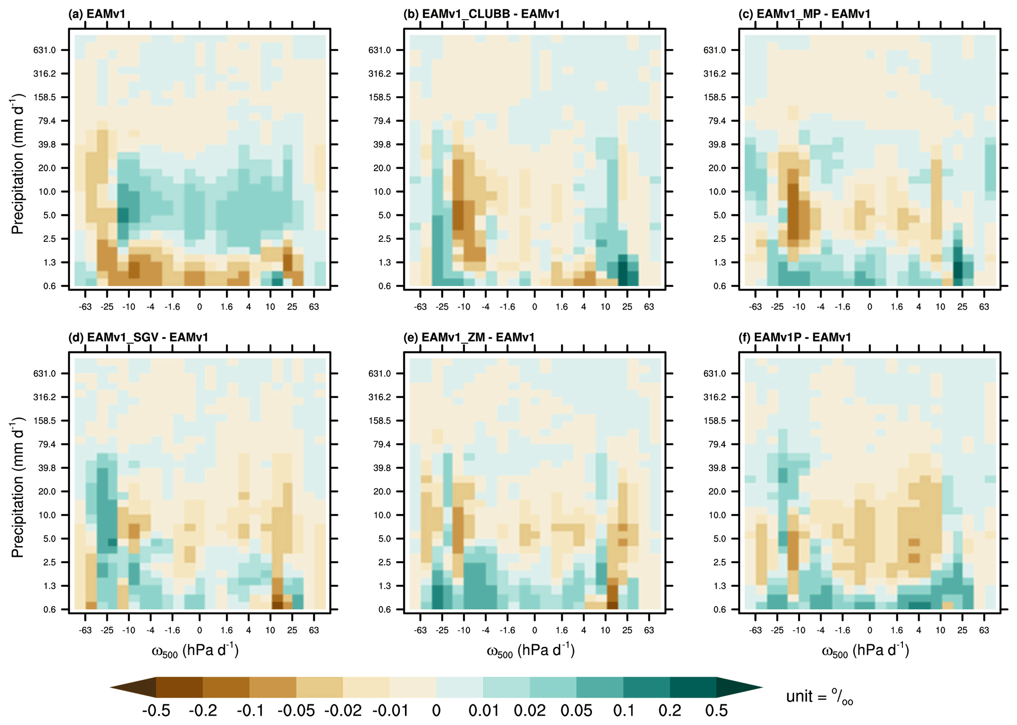
Figure 16Anthropogenic aerosol-induced change in frequency of occurrence of resolved-scale precipitation as a function of vertical velocity at 500 hPa (unit = hPa d−1) in (a) EAMv1 and differences between (b) EAMv1_CLUBB and EAMv1, (c) EAMv1_MP and EAMv1, (d) EAMv1_SGV and EAMv1, (e) EAMv1_ZM and EAMv1, and (f) EAMv1P and EAMv1. Model precipitation rates are sampled at every model time step (dt=30 min).
In summary, the recalibration reduces the overall responses of CREs, surface temperature, and the hydrological cycle to aerosols. Evaluation of the hydrological cycle response to aerosols indicates that the total precipitation rate is influenced globally (Table 9), regionally (not shown), and in terms of large-scale precipitation frequency of occurrence (using a joint PDF; Fig. 16). However, the global mean ERFant, ERFaer, and ERFaci remain about the same between the default model EAMv1 and the recalibrated model EAMv1P due to invariant effects of changes in Nc, and due to compensations in shortwave and longwave effects that vary in the opposite direction. These analyses demonstrate that the global mean ERFs are insufficient for understanding or constraining the response of the hydrological cycle and surface temperature to aerosols. The shortwave and longwave contribution to the total aerosol ERF, as well as the spatial distribution of aerosol ERF, need to be considered to understand how aerosols affect the Earth system. Furthermore, the unperturbed base state climate can play a role as well. As shown in Fig. 10, the recalibrated model reduces the surface temperature bias significantly, which can lead to a more realistic response of surface temperature to forcings.
3.5 Response to surface warming
The response of the Earth system to surface warming is of great scientific and societal importance. ECS values in CMIP6 span a significantly wider range (1.8 to 5.6 K) than in CMIP5 and observationally constrained estimates (Sherwood et al., 2020), and their substantially higher multi-model mean value has been attributed to the same causes identified in E3SMv1: strong positive cloud feedbacks (Zelinka et al., 2020). In this section, we discuss the impacts of parameter adjustments on cloud and other climate feedbacks. The feedbacks are assessed using the Cess methodology (Cess et al., 1989) by contrasting the difference between a control pre-industrial simulation and a perturbed simulation with SST elevated by 4 K globally (see Sect. 2 for the experiment design).
Figure 17 shows that EAMv1's total climate feedback of −1.51 W m−2 K−1 is weaker than the CMIP5 multi-model mean (−1.6 W m−2 K−1), but it is within the inter-model spread of −1.05 to −1.95 W m−2 K−1 (Ringer et al., 2014). The less negative feedback suggests a faster warming in the late 20th century and a higher ECS, consistent with the findings in Golaz et al. (2019). EAMv1_CLUBB and EAMv1_MP produce stronger global mean feedback, which will lead to lower ECS and weaker warming in the 20th century, while EAMv1_ZM produces positive feedback in the tropics. The recalibrated model EAMv1P produces a stronger climate feedback of −1.74 W m−2 K−1, a 15 % increase from EAMv1, and thus it can be expected to have a lower ECS.
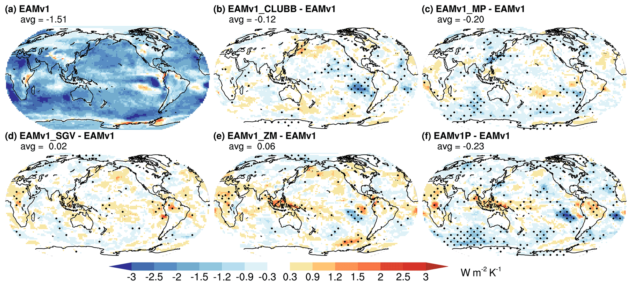
Figure 17Climate feedback parameter (Cess et al., 1989).
In Fig. 18, climate feedbacks diagnosed using the Pendergrass et al. (2018) radiative kernel reveal that the non-cloud feedbacks are invariant across different model configurations and that the variation in total climate feedback is due solely to the spread in cloud feedbacks as a result of our parameter and subgrid adjustments. Further decomposing the cloud feedback into its total, shortwave, and longwave components via cloud radiative kernels (Zelinka et al., 2012a, b, 2013) indicates that cloud feedbacks are weakened from 0.77, 0.35, and 0.42 W m−2 K−1 in EAMv1 to 0.47 (−39 %), 0.20 (−43 %), and 0.27 W m−2 K−1 (−35 %) in EAMv1P. The stronger negative total climate feedback from the weakened positive cloud feedback suggests that the recalibration will produce a slower warming in the late 20th century and lower ECS.
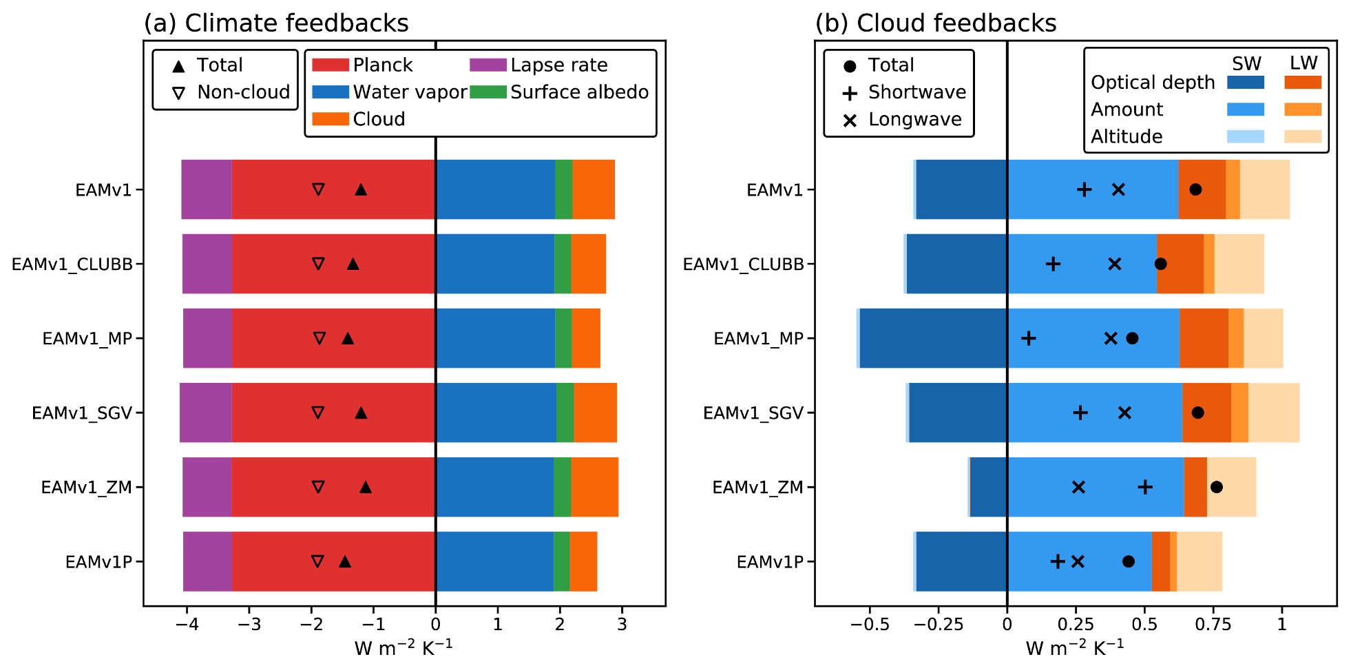
Figure 18(a) Climate feedbacks and (b) cloud feedbacks decomposed using radiative kernels (Pendergrass et al., 2018; Zelinka et al., 2012b, a, 2013).
Figure 18b shows that EAMv1_CLUBB and EAMv1_MP both reduce the magnitude of shortwave cloud feedback. EAMv1_MP strengthens the negative shortwave cloud optical depth feedback, likely due to the reduction of mean-state supercooled liquid in mixed-phase clouds (by strengthening the WBF process). The weaker cloud feedback in EAMv1_CLUBB comes from the reduction of cloud amount feedback. This is likely due to the fact that EAMv1_CLUBB improves the simulation of shallow Cu. Because Sc cloud amount decreases more with warming than shallow Cu (Cesana et al., 2019; Cesana and Del Genio, 2021; Myers et al., 2021; Scott et al., 2020), producing shallow Cu rather than Sc reduces cloud amount feedback. In other words, EAMv1_CLUBB simulates a control-state climate with more Cu and less Sc than the default EAMv1, and thus the positive feedback from warming-induced reductions of low-cloud cover is weakened because Cu is more resilient to warming than Sc. In the meantime, EAMv1_CLUBB reduces the decoupling strength and cloud-top entrainment in the Sc regime, which can also reduce the cloud amount feedback.
Contrary to the effects introduced by EAMv1_CLUBB and EAMV1_MP, EAMv1_ZM enhances total cloud feedback. Figure 18b shows that EAMv1_ZM significantly reduces both shortwave and longwave cloud optical depth feedbacks and diminishes longwave cloud amount feedback. The large reduction in the negative shortwave cloud optical depth feedback results in a stronger positive total cloud feedback. This indicates that changes made in EAMv1_ZM, particularly (1) the reduction of the ice particle radius detrained from deep convection (ice_deep) and (2) the reduction of convective autoconversion (c0_ocn and c0_lnd), which make convective clouds and their anvils opaque in the present-day climate, result in a weaker sensitivity of CRE to surface warming. However, the physical mechanisms relating those tuning choices to cloud feedbacks remain unclear and require further investigation.
Figure 19 shows that parameter adjustments affect cloud feedbacks in different geographical regions. The total cloud feedback appears to be a balance between cloud optical depth feedback and cloud amount feedback, as the cloud altitude feedback is insensitive to our adjustments in parameters and subgrid effects. In the tropics, the recalibrated model EAMv1P shows stronger positive total cloud feedback (Fig. 19a), which can be attributed to the enhanced cloud optical depth feedback introduced by EAMv1_SGV and EAMv1_ZM. This highlights the importance of realistic representation of cloud properties associated with deep convection, including both the deep convective clouds and the anvil detrained from deep convection. In the subtropics, EAMv1P produces weaker positive total cloud feedback due to the reduction of cloud amount feedback in EAMv1_CLUBB and EAMv1_ZM. EAMv1_CLUBB weakens turbulent mixing and increases the skewness Skw in the shallow Cu regions to facilitate asymmetric vertical mixing that enhances shallow Cu rather than the symmetric vertical mixing that enhances Sc. For this reason, a weaker positive cloud feedback is expected since Sc cloud amount decreases more with warming than shallow Cu (Cesana et al., 2019). EAMv1_ZM also reduces subtropical cloud amount feedback, likely through its impacts on circulation that affect subtropical subsidence and clouds. In midlatitudes and high latitudes, EAMv1_MP makes the largest contribution to modifying cloud feedbacks. Making the WBF process more efficient reduces supercooled liquid clouds in the mean state, which strengthens the negative cloud optical depth feedback through enhancing the negative cloud-phase feedback (Tan et al., 2016). We note that the high-latitude cloud optical depth feedback is highly uncertain. Sherwood et al. (2020) estimated the feedback to be near zero based on two studies, Ceppi et al. (2016) and Terai et al. (2016), which reported feedback estimates of similar magnitude but opposite signs. Hence, it remains unclear if the stronger negative cloud optical depth feedback in the Southern Ocean produced by EAMv1_MP and EAMv1P is closer to reality, but this essentially reduces the global total cloud feedback due to the sign reversal of the total cloud feedback in the Southern Ocean.
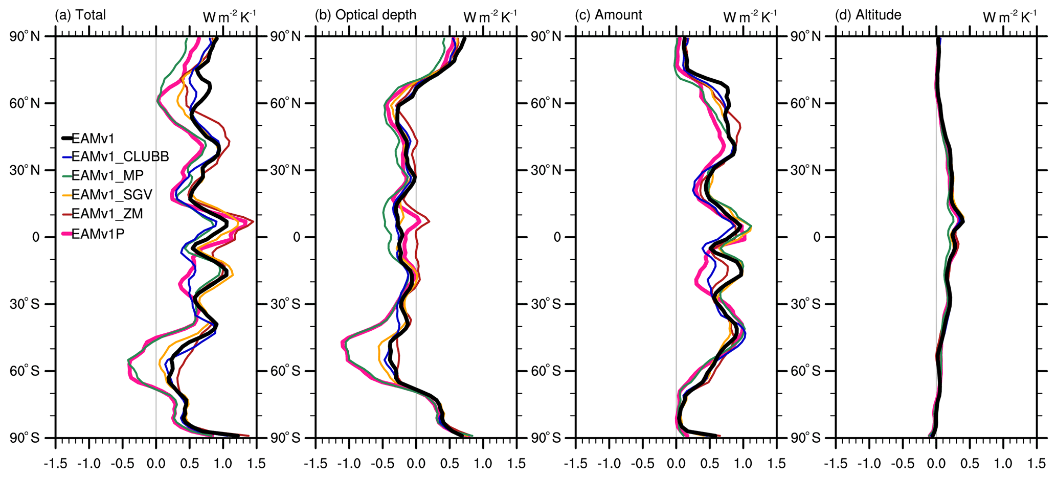
Figure 19Zonal mean of (a) total cloud feedback, (b) cloud optical depth feedback, (c) cloud amount feedback, and (d) cloud altitude feedback.
In Table 11, we find that cloud fraction changes induced by surface warming are insensitive to the recalibration. LWP increases as the surface warms. By making the WBF process more efficient, EAMv1_MP shows a greater LWP response to surface warming, which weakens the positive cloud feedback as discussed previously. Liquid and ice particle numbers Nc and Ni are both reduced with surface warming, and parameter adjustments in EAMv1_MP and EAMv1_ZM affect the sensitivity. In terms of radiative properties, we find that the recalibration reverses the sign of the response of τliq to surface warming largely due to the changes made in EAMv1_MP, leading to cloud thickening instead of thinning in the lower troposphere (i.e., increasing τlow as surface warms). In the upper troposphere, EAMv1_ZM reduces the τhgh sensitivity to surface warming, which weakens the positive high cloud feedback. The modifications in EAMv1_ZM have the largest impact on the changes in CRE response changes associated with ice clouds. Combining all of the changes, the revised model EAMv1P reverses the sign of the liquid CREs, likely due to the cloud-phase response to warming caused by increased IWP in the model.
Table 11The same as Table 6 but showing the change in cloud properties induced by surface warming relative to their pre-industrial values (unit = % K−1). Variables are defined in Table 6.
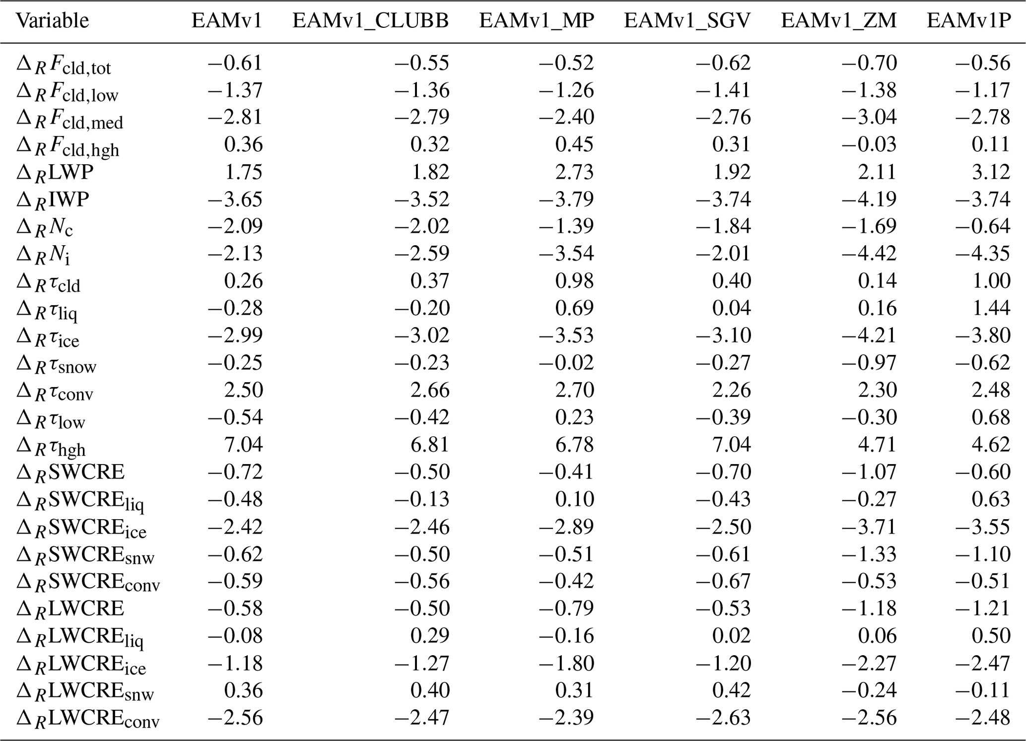
In assessing the impact of parameter changes on ECS, we also computed the lower tropospheric mixing index (LTMI) (Sherwood et al., 2014) and found that the recalibration leads to a 10 % reduction in LTMI (not shown), which corresponds to about 1 K decrease in ECS based on the LTMI–ECS relationship from CMIP5. Most parameter adjustments do not alter LTMI. EAMv1_ZM produces lower LTMI because it reduces convective activity by weakening the convective autoconversion process to increase the cirrus cloud opacity that stabilizes the troposphere. However, because the statistical significance of the relationship between LTMI and ECS has decreased in CMIP6 compared to CMIP5 (Schlund et al., 2020), LTMI might not be a good predictor for ECS in E3SM.
Finally, we assess the impacts of our recalibration on the patterned response of precipitation to surface warming. In Sect. 3.2 we showed that the parameter changes in EAMv1_ZM significantly reduce the ratio of convective precipitation rate to total precipitation rate in the present-day climatology. This change alone can lead to different precipitation responses to surface warming because different precipitation mechanisms are employed between the convection and the microphysics parameterizations. Figure 20 shows enhanced convective precipitation with warming in the tropics, the SPCZ, and storm tracks in EAMv1. EAMv1_ZM significantly reduces the response, likely due to the reduced convective autoconversion efficiency. Other parameter adjustments also affect the response in the Indo-Pacific warm pool, but the parameter changes do not have a direct impact on convective precipitation, and thus the change in response might be caused by circulation feedbacks. In the recalibrated model EAMv1P, the convective precipitation response to surface warming is mostly reduced in the tropics. The global mean convective precipitation response is reduced by 0.013 mm d−1 K−1 (−24 %) compared to the response in EAMv1. The relative increase in convective precipitation due to surface warming, however, is only slightly reduced from 3.07 % K−1 in EAMv1 to 2.97 % K−1 in EAMv1P.
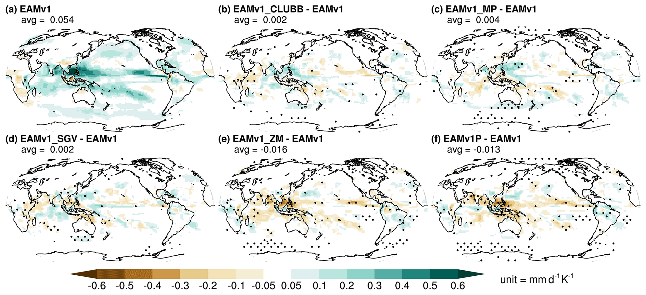
Figure 20The change in convective precipitation rate induced by surface warming.
The large-scale precipitation response in EAMv1 has a similar magnitude as the convective precipitation response, but the response is larger in the storm tracks and not as strong in the tropics (Fig. 21). EAMv1_ZM significantly enhances the response in the TWP because the parameter changes in EAMv1_ZM shift the precipitation from convective to large-scale so that the response comes from the large-scale precipitation. The recalibrated model EAMv1P enhances the large-scale precipitation response by 0.018 mm d−1 K−1 (+37 %) compared to EAMv1. The relative increase in large-scale precipitation due to surface warming is also increased from 3.17 % K−1 in EAMv1 to 4.11 % K−1 in EAMv1P.
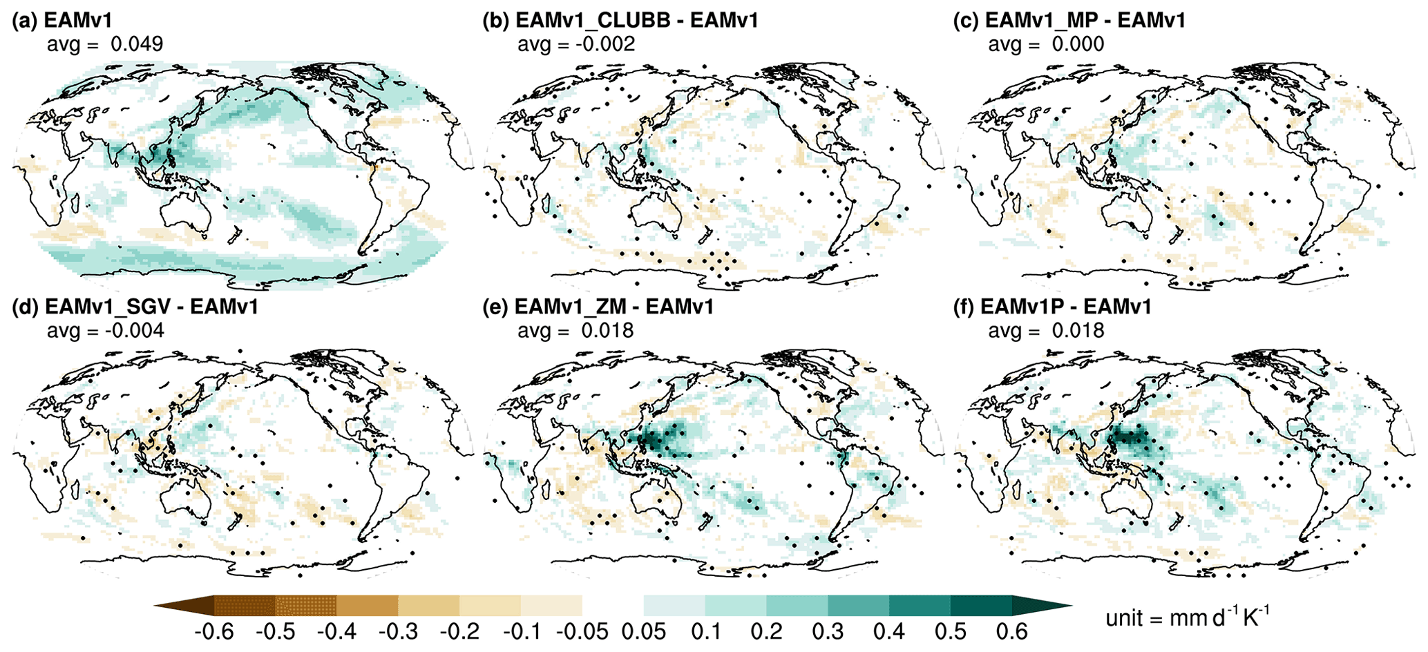
Figure 21The change in large-scale precipitation rate induced by surface warming.
In summary, the recalibration enhances the negative climate feedback to surface warming by reducing the positive cloud feedback. The storm track, shallow Cu regions, and the Indo-Pacific warm pool are the regions where the cloud feedback is most sensitive to the parameter adjustments. The largest precipitation response is seen in the tropics, SPCZ, and storm tracks. The parameter adjustments in the ZM deep-convection parameterization produce the largest changes in the response. Because the default model EAMv1 and the recalibrated model EAMv1P produce different climate and cloud feedbacks, the two models are expected to produce different estimates of ECS, even though their ERFant values are about the same. Our results are consistent with the findings of Smith et al. (2020) that the statistical relationship between the ERFaer and ECS established in Kiehl (2007) and Forster et al. (2013) is challenged by modern ESMs. Fully coupled model simulations are needed to test this hypothesis.
In this study, we have developed a new model configuration of EAMv1, named EAMv1P, using a model calibration strategy that focuses on calibrating CREs that can be reliably observed across cloud regimes and geographical regions. The recalibration was guided by our understanding of the physical mechanisms that relate biases to uncertain process assumptions and used ample iterations to buffer unintended consequences of interventions in individual regimes against those they interact with. The recalibrated model produces an encouragingly improved present-day cloud and precipitation climatology and reduced sensitivity to aerosol perturbation and surface warming. Below we summarize the changes and behavior of the intermediate model configurations.
-
Incorporating the subgrid effects (EAMv1_SGV) was intended to increase cloudiness in regions where large-scale winds are weak and yet convection occurs frequently (e.g., TWP and Amazon) by enhancing local surface fluxes of heat, moisture, and momentum in those regions. Compared to all other intermediate model configurations, EAMv1_SGV produces the largest impact in terms of reducing the tropical surface wind direction bias, which will likely reduce the cold tongue bias in the fully coupled E3SM. Introducing these subgrid effects also reduces precipitation biases over the TWP, Amazon, and high-elevation regions (e.g., the Himalayas and Andes). EAMv1_SGV produces only a moderately weakened surface temperature response and precipitation response to aerosol forcing compared to the default model EAMv1.
-
Parameter adjustments in the ZM deep-convection parameterization (EAMv1_ZM) were intended to improve overall tropical cloud amounts by weakening the convective autoconversion and reducing detrained ice crystal radius. We find that these changes increase IWP globally. Furthermore, we find that EAMv1_ZM is the only model configuration that produces a stronger ERFaci and a stronger positive cloud feedback. The enhanced ERFaci is seen in East Asia, Europe, and Sc and shallow Cu regions. The increased cloud feedback is primarily due to the significant reduction of negative cloud optical depth feedback in the tropics.
-
Parameter adjustments in the CLUBB parameterization (EAMv1_CLUBB) were introduced to improve the subtropical Sc, shallow Cu, and the Sc-to-Cu transition by making parameters a function of the skewness of subgrid vertical velocity Skw. These changes lead to encouraging reductions in both the “too-dim stratocumulus” and “too-bright trade cumulus” biases in modern ESMs. We find that the changes also significantly reduce the precipitation bias over the central Pacific Ocean. The changes introduced in EAMv1_CLUBB do not affect ERFaci, but they lead to the largest reduction in the positive cloud amount feedback in the subtropics compared to other intermediate model configurations.
-
Parameter adjustments in the MG2 microphysical parameterization (EAMv1_MP) were intended to (1) reduce the excessive supercooled cloud liquid in the midlatitudes and high latitudes by enhancing the WBF process, (2) reduce ice particle number by reducing the sulfate aerosol available for homogeneous ice nucleation, and (3) improve Sc by enhancing the droplet sedimentation rate. We find that these changes give the largest reduction in ERFaci in the midlatitudes and high latitudes, in areas under great anthropogenic influence (e.g., East Asia, North America), and in the subtropics. EAMv1_MP also produces the weakest total cloud feedback due to the stronger negative cloud optical depth feedback in the tropics, midlatitudes, and high latitudes. The significant enhancement of negative cloud optical depth feedback results in a reversal of the sign of the total cloud feedback in the Southern Ocean.
The revised model EAMv1P includes all of the incremental changes discussed above. We find that EAMv1P produces a much more realistic CRE distribution than EAMv1 by addressing multiple regime-specific cloud biases spanning the tropics, subtropics, midlatitudes, and high latitudes. This is achieved through the collective effects of our modest adjustments to the ZM deep-convection scheme and subgrid effects, CLUBB turbulence, and MG2 microphysics. The improved CRE distribution naturally leads to better geographic distribution of radiative energy at the TOA, which is essential for setting up a realistic atmospheric circulation that further improves the overall fidelity of the model atmospheric state. We have also compared results from grouped parameter changes to understand how process assumptions affect CRE and other aspects of the simulated atmosphere. We show that the recalibrated model produces more improvements than the sum of the improvements from individual intermediate configuration, demonstrating the nonlinearity in the climate system and the necessity of combining all of the improvements that target different biases in different regimes. Further reducing the model biases by improving parameterizations, numerics, resolution, and calibration is an ongoing effort for the E3SM team. Incorporating process-oriented diagnostics in model development and calibration will be useful for ensuring that the model get the right answer for the right reason.
Cloud, precipitation, and surface temperature responses to anthropogenic aerosols and greenhouse gases are major sources of uncertainty in the simulated climate of the past, present, and future. Since the climate system is nonlinear, realistic estimates of the system's response depend on a realistic base state. EAMv1's deficiencies in base state fidelity likely contribute to its biases in the historical surface temperature evolution and its high ECS. In contrast, the recalibrated model EAMv1P produces a much more realistic present-day base climate state, due to a better calibration of cloud properties and subgrid effects that improve the representation of physical mechanisms compared to EAMv1. Hence, the revised model EAMv1P is more likely to produce credible estimates of the climate system's response to external forcings and climate projections when running as part of the fully coupled E3SM.
We show that the sensitivity of clouds, precipitation, and surface temperature to anthropogenic aerosols is significantly lower in the recalibrated model than in the default model, suggesting the potential to improve the historical surface temperature evolution over E3SMv1, such as the potential to reduce the cold bias between the 1960s and 1980s. We find that the responses to anthropogenic aerosols are mostly affected by parameter adjustments in EAMv1_MP and EAMv1_ZM. To simulate historical surface temperature evolution accurately, future model development efforts should target these two parameterizations so that processes of cloud microphysical and deep convective processes are better constrained to represent real-world processes.
The recalibrated model EAMv1P also produces a weaker cloud feedback compared to the default model EAMv1, suggesting potential improvements to the surface temperature evolution, like slower warming after the 1980s and a lower ECS. Parameter adjustments in EAMv1_CLUBB, EAMv1_MP, and EAMv1_ZM significantly affect cloud feedbacks. Hence, to reduce the uncertainty in the predictions of future climate, subgrid cloud properties and process representations, including turbulent mixing, cloud macrophysics and microphysics, and deep convection, need to be better constrained. We find that EAMv1 and EAMv1P produce different surface temperature responses to anthropogenic aerosols and different cloud feedbacks (and, consequently, ECS) even though they produce the same global mean ERF. This suggests that the statistical relationships between the global mean ERF, cloud feedback, and ECS established in Kiehl (2007) and Forster et al. (2013) do not apply to current generation ESMs, as documented in Smith et al. (2020). This indicates that global mean ERF is not a good indicator of the historical and future climate change. Other factors such as the spectral composition (i.e., shortwave versus longwave) and spatial distribution of the ERF and cloud feedback, as well as the realism of the unperturbed base climate state, need to be considered. Identifying the process representations that affect only ERF, those that affect only cloud feedback, and those that affect both is an important step toward a better understanding of the evolution of the climate system.
It is natural to wonder if an equivalent or superior ESM calibration might have been achievable with less human effort or fewer computational resources via semi-automated machine learning (ML) methods that emulate or expand the workflow outlined in this paper. Indeed, emulating a complex model's parameter sensitivities following human-constructed trial simulations to aid model calibration and uncertainty quantification would be an intriguing possibility. Several recent studies have shown successful application of ML methods in model calibration (Cleary et al., 2021; Dunbar et al., 2021; Couvreux et al., 2021; Hourdin et al., 2021). In theory, reinforcement learning (RL) with an appropriately formulated agent-based optimization system could be guided via its loss function formulation with skill metrics that optimize for the same patterns and mean-state climate metrics that we prioritized in this study. In practice, however, this ML task faces a fundamental challenge that the cost of an individual agent–reward sample is performing multi-year climate simulations. The workflow outlined in this paper has the considerable advantage that experienced human experts make educated parameter interventions based on assessment of the simulation and discriminate the desired effects in a nuanced way that tolerates certain unintended consequences. It is not clear how available ML methods could be infused with analogous physical foresight to make similar decisions, and thus it is logical to expect that they would require more evaluation samples to succeed via brute force. Therefore, experimenting with clever strategies to increase reward density and to integrate physical knowledge from experts in the ML workflow would be a highly worthwhile long-term challenge.
The E3SM model code and input data are available at https://doi.org/10.11578/E3SM/dc.20180418.36 (E3SM Project, DOE, 2018). The model simulation data used in this study are available at https://portal.nersc.gov/archive/home/p/plma/www/eamv1_tunings (Ma, 2021a). The ERA5 data are obtained from Copernicus Climate Change Service Climate Data Store (CDS) access on 27 December 2019, at https://doi.org/10.24381/cds.6860a573 (Hersbach et al., 2019b). The CERES-EBAF cloud radiative effect data are obtained at https://ceres-tool.larc.nasa.gov/ord-tool/jsp/EBAFTOA41Selection.jsp (Loeb et al., 2018). The GPCP precipitation data are obtained from NOAA/OAR/ESRL PSL at https://psl.noaa.gov/data/gridded/data.gpcp.html (Adler et al, 2018). The MODIS data are obtained from NASA GIOVANNI at https://giovanni.gsfc.nasa.gov/giovanni/ (NASA, 2021a). The MERRA-2 dataset is obtained from NASA Goddard Earth Sciences (GES) Data and Information Services Center (DISC) at https://disc.gsfc.nasa.gov/ (NASA, 2021b). The GOCCP data are obtained from https://climserv.ipsl.polytechnique.fr/cfmip-obs/ (Bony et al., 2021). The E3SM diagnostics package used in this study was archived at https://doi.org/10.5281/zenodo.5555094 (Ma, 2021b).
PLM designed the study, performed simulations and analyses, and prepared the first draft of the manuscript. BEH, VEL, RBN, AG, HM, HaW, KZ, PAB, ZZ, HS, XL, JW, PMC, and PJR contributed to developing the tuning strategy and analysis. SAK, MDZ, and YZ performed the cloud feedback decomposition analysis and contributed to cloud evaluation. YQ, JHY, CRJ, MH, SLT, XueZ, WL, JQ, HC, MAB, JM, SH, QT, and JF contributed to the evaluation and analysis of results. BS implemented the code in E3SMv1. XubZ, LKB, and JDF contributed to assessment of subgrid effects. HuW and MAT contributed to the testing of model sensitivity to time-stepping and process coupling. MSP contributed to the analysis of results and the assessment of using machine learning methods for tuning. JCG, SX, and LRL contributed to interpreting results and the comparisons with other modeling studies. All authors contributed to the writing of the manuscript.
At least one of the (co-)authors is a member of the editorial board of Geoscientific Model Development. The peer-review process was guided by an independent editor, and the authors also have no other competing interests to declare.
Publisher's note: Copernicus Publications remains neutral with regard to jurisdictional claims in published maps and institutional affiliations.
The model tuning work was supported as part of the Energy Exascale Earth System Model (E3SM) project (project no. 65814). The analyses of effective radiative forcing and aerosol–cloud interactions were supported as part of the Enabling Aerosol–cloud interactions at GLobal convection-permitting scalES (EAGLES) project (project no. 74358). The E3SM and EAGLES projects were sponsored by the U.S. Department of Energy, Office of Science, Office of Biological and Environmental Research, Earth System Model Development (ESMD) program area. The cloud diagnostics and feedback analysis were supported as part of a cloud diagnostics project (project no. 66187) and Program for Climate Model Diagnosis & Intercomparison (PCMDI) (project no. SCW1453), respectively, both sponsored by the U.S. Department of Energy, Office of Science, Office of Biological and Environmental Research, Regional and Global Model Analysis (RGMA) program area. The development and evaluation of gustiness effects over land were part of the Integrated Cloud, Land-Surface, and Aerosol System Study (ICLASS) science focus area (project no. 57131), sponsored by the U.S. Department of Energy, Office of Science, Office of Biological and Environmental Research, Atmospheric System Research (ASR) program. This research used resources of the National Energy Research Scientific Computing Center (NERSC), a U.S. Department of Energy Office of Science User Facility operated under contract no. DE-AC02-05CH11231. This research also used a high-performance computing cluster provided by the Office of Biological and Environmental Research, ESMD program area, and operated by the Laboratory Computing Resource Center at Argonne National Laboratory. This paper describes objective technical results and analysis. Any subjective views or opinions that might be expressed in the paper do not necessarily represent the views of the U.S. Department of Energy or the United States Government.
This study was funded by the U.S. Department of Energy, Office of Science, Office of Biological and Environmental Research, Earth System Model Development (ESMD) program area (project nos. 65814, 74358); Regional and Global Model Analysis (RGMA) program area (project nos. 66187, SCW1453); and Atmospheric System Research (ASR) program (project no. 57131). The Pacific Northwest National Laboratory is operated for the U.S. Department of Energy by the Battelle Memorial Institute under contract DE-AC05-76RL01830. Work at Lawrence Livermore National Laboratory was performed under the auspices of the U.S. Department of Energy by Lawrence Livermore National Laboratory under contract no. DE-AC52-07NA27344. Sandia National Laboratories is a multi-mission laboratory managed and operated by National Technology & Engineering Solutions of Sandia, LLC, a wholly owned subsidiary of Honeywell International Inc., for the U.S. Department of Energy's National Nuclear Security Administration under contract no. DE-NA0003525.
This paper was edited by Axel Lauer and reviewed by Yuan Wang and two anonymous referees.
Adler, R., Sapiano, M., Huffman, G., Wang, J.-J., Gu, G., Bolvin, D., Chiu, L., Schneider, U., Becker, A., Nelkin, E., Xie, P., Ferraro, R., and Shin, D.-B.: The Global Precipitation Climatology Project (GPCP) Monthly Analysis (New Version 2.3) and a Review of 2017 Global Precipitation, Atmosphere, 9, 138, https://doi.org/10.3390/atmos9040138, 2018 (data available at: https://psl.noaa.gov/data/gridded/data.gpcp.html, last access: 20 December 2021).
Bellouin, N., Quaas, J., Gryspeerdt, E., Kinne, S., Stier, P., Watson-Parris, D., Boucher, O., Carslaw, K. S., Christensen, M., Daniau, A. L., Dufresne, J. L., Feingold, G., Fiedler, S., Forster, P., Gettelman, A., Haywood, J. M., Lohmann, U., Malavelle, F., Mauritsen, T., McCoy, D. T., Myhre, G., Mulmenstadt, J., Neubauer, D., Possner, A., Rugenstein, M., Sato, Y., Schulz, M., Schwartz, S. E., Sourdeval, O., Storelvmo, T., Toll, V., Winker, D., and Stevens, B.: Bounding Global Aerosol Radiative Forcing of Climate Change, Rev. Geophys., 58, e2019RG000660, https://doi.org/10.1029/2019RG000660, 2020.
Bodas-Salcedo, A., Webb, M. J., Bony, S., Chepfer, H., Dufresne, J. L., Klein, S. A., Zhang, Y., Marchand, R., Haynes, J. M., Pincus, R., and John, V. O.: COSP Satellite simulation software for model assessment, B. Am. Meteorol. Soc., 92, 1023–1043, https://doi.org/10.1175/2011bams2856.1, 2011.
Bogenschutz, P. A., Gettelman, A., Morrison, H., Larson, V. E., Craig, C., and Schanen, D. P.: Higher-Order Turbulence Closure and Its Impact on Climate Simulations in the Community Atmosphere Model, J. Climate, 26, 9655–9676, https://doi.org/10.1175/Jcli-D-13-00075.1, 2013.
Bony, S., Chepfer, H., Chiriaco, M., Dufresne, J.-L., Klein, S., Loeb, N., Marchand, R., Pincus, R., Tanré, D., Webb, M., Winker, D., Xie, S., and Zhang, Y.: CFMIP Observations for Model evaluation, CFMIP-OBS [data set], https://climserv.ipsl.polytechnique.fr/cfmip-obs/, last access: 10 December 2021.
Boucher, O., Randall, D., Artaxo, P., Bretherton, C., Feingold, G., Forster, P., Kerminen, V. M., Kondo, Y., Liao, H., Lohmann, U., Rasch, P., Satheesh, S. K., Sherwood, S., Stevens, B., and Zhang, X. Y.: Clouds and Aerosols. In: Climate Change 2013: The Physical Science Basis. Contribution of Working Group I to the Fifth Assessment Report of the Intergovernmental Panel on Climate Change, edited by: Stocker, T. F., Qin, D., Plattner, G.-K., Tignor, M., Allen, S. K., Boschung, J., Nauels, A., Xia, Y., Bex, V., and Midgley, P. M., Cambridge University Press, Cambridge, United Kingdom and New York, NY, USA, https://doi.org/10.1017/CBO9781107415324.016, 2013.
Bretherton, C. S., Blossey, P. N., and Uchida, J.: Cloud droplet sedimentation, entrainment efficiency, and subtropical stratocumulus albedo, Geophys. Res. Lett., 34, L03813, https://doi.org/10.1029/2006gl027648, 2007.
Brunke, M. A., Ma, P. L., Eyre, J. E. J. R., Rasch, P. J., Sorooshian, A., and Zeng, X. B.: Subtropical Marine Low Stratiform Cloud Deck Spatial Errors in the E3SMv1 Atmosphere Model, Geophys. Res. Lett., 46, 12598–12607, https://doi.org/10.1029/2019gl084747, 2019.
Burrows, S. M., Dasgupta, A., Reehl, S., Bramer, L., Ma, P. L., Rasch, P. J., and Qian, Y.: Characterizing the Relative Importance Assigned to Physical Variables by Climate Scientists when Assessing Atmospheric Climate Model Fidelity, Adv. Atmos. Sci., 35, 1101–1113, https://doi.org/10.1007/s00376-018-7300-x, 2018.
Caldwell, P. M., Mametjanov, A., Tang, Q., Van Roekel, L. P., Golaz, J. C., Lin, W. Y., Bader, D. C., Keen, N. D., Feng, Y., Jacob, R., Maltrud, M. E., Roberts, A. F., Taylor, M. A., Veneziani, M., Wang, H. L., Wolfe, J. D., Balaguru, K., Cameron-Smith, P., Dong, L., Klein, S. A., Leung, L. R., Li, H. Y., Li, Q., Liu, X. H., Neale, R. B., Pinheiro, M., Qian, Y., Ullrich, P. A., Xie, S. C., Yang, Y., Zhang, Y. Y., Zhang, K., and Zhou, T.: The DOE E3SM Coupled Model Version 1: Description and Results at High Resolution, J. Adv. Model. Earth Sy., 11, 4095–4146, https://doi.org/10.1029/2019ms001870, 2019.
Carslaw, K. S., Lee, L. A., Reddington, C. L., Pringle, K. J., Rap, A., Forster, P. M., Mann, G. W., Spracklen, D. V., Woodhouse, M. T., Regayre, L. A., and Pierce, J. R.: Large contribution of natural aerosols to uncertainty in indirect forcing, Nature, 503, 67–71, https://doi.org/10.1038/nature12674, 2013.
Ceppi, P., McCoy, D. T., and Hartmann, D. L.: Observational evidence for a negative shortwave cloud feedback in middle to high latitudes, Geophys. Res. Lett., 43, 1331–1339, https://doi.org/10.1002/2015gl067499, 2016.
Cesana, G. and Chepfer, H.: Evaluation of the cloud thermodynamic phase in a climate model using CALIPSO-GOCCP, J. Geophys. Res.-Atmos., 118, 7922–7937, https://doi.org/10.1002/jgrd.50376, 2013.
Cesana, G., Waliser, D. E., Jiang, X., and Li, J. L. F.: Multimodel evaluation of cloud phase transition using satellite and reanalysis data, J. Geophys. Res.-Atmos., 120, 7871–7892, https://doi.org/10.1002/2014jd022932, 2015.
Cesana, G., Del Genio, A. D., Ackerman, A. S., Kelley, M., Elsaesser, G., Fridlind, A. M., Cheng, Y., and Yao, M.-S.: Evaluating models' response of tropical low clouds to SST forcings using CALIPSO observations, Atmos. Chem. Phys., 19, 2813–2832, https://doi.org/10.5194/acp-19-2813-2019, 2019.
Cesana, G. V., and Del Genio, A. D.: Observational constraint on cloud feedbacks suggests moderate climate sensitivity, Nat. Clim. Change, 11, 213–218, https://doi.org/10.1038/s41558-020-00970-y, 2021.
Cess, R. D., Potter, G. L., Blanchet, J. P., Boer, G. J., Ghan, S. J., Kiehl, J. T., Letreut, H., Li, Z. X., Liang, X. Z., Mitchell, J. F. B., Morcrette, J. J., Randall, D. A., Riches, M. R., Roeckner, E., Schlese, U., Slingo, A., Taylor, K. E., Washington, W. M., Wetherald, R. T., and Yagai, I.: Interpretation of Cloud-Climate Feedback as Produced by 14 Atmospheric General-Circulation Models, Science, 245, 513–516, https://doi.org/10.1126/science.245.4917.513, 1989.
Chepfer, H., Bony, S., Winker, D., Chiriaco, M., Dufresne, J. L., and Seze, G.: Use of CALIPSO lidar observations to evaluate the cloudiness simulated by a climate model, Geophys. Res. Lett., 35, L15704, https://doi.org/10.1029/2008gl034207, 2008.
Chepfer, H., Bony, S., Winker, D., Cesana, G., Dufresne, J. L., Minnis, P., Stubenrauch, C. J., and Zeng, S.: The GCM-Oriented CALIPSO Cloud Product (CALIPSO-GOCCP), J. Geophys. Res.-Atmos., 115, D00H16, https://doi.org/10.1029/2009jd012251, 2010.
Cleary, E., Garbuno-Inigo, A., Lan, S. W., Schneider, T., and Stuart, A. M.: Calibrate, emulate, sample, J. Comput. Phys., 424, 109716, https://doi.org/10.1016/j.jcp.2020.109716, 2021.
Couvreux, F., Hourdin, F., Williamson, D., Roehrig, R., Volodina, V., Villefranque, N., Rio, C., Audouin, O., Salter, J., Bazile, E., Brient, F., Favot, F., Honnert, R., Lefebvre, M. P., Madeleine, J. B., Rodier, Q., and Xu, W. Z.: Process-Based Climate Model Development Harnessing Machine Learning: I. A Calibration Tool for Parameterization Improvement, J. Adv. Model. Earth Sy., 13, e2020MS002217, https://doi.org/10.1029/2020MS002217, 2021.
Dai, A.: Precipitation characteristics in eighteen coupled climate models, J. Climate, 19, 4605–4630, https://doi.org/10.1175/Jcli3884.1, 2006.
DeMott, P. J., Prenni, A. J., Liu, X., Kreidenweis, S. M., Petters, M. D., Twohy, C. H., Richardson, M. S., Eidhammer, T., and Rogers, D. C.: Predicting global atmospheric ice nuclei distributions and their impacts on climate, P. Natl. Acad. Sci. USA, 107, 11217–11222, https://doi.org/10.1073/pnas.0910818107, 2010.
Dunbar, O. R. A., Garbuno-Inigo, A., Schneider, T., and Stuart, A. M.: Calibration and Uncertainty Quantification of Convective Parameters in an Idealized GCM, J. Adv. Model. Earth Sy., 13, e2020MS002454, https://doi.org/10.1029/2020MS002454, 2021.
E3SM Project, DOE: Energy Exascale Earth System Model v1.0, DOE [code], https://doi.org/10.11578/E3SM/dc.20180418.36, 2018.
Forster, P. M., Andrews, T., Good, P., Gregory, J. M., Jackson, L. S., and Zelinka, M.: Evaluating adjusted forcing and model spread for historical and future scenarios in the CMIP5 generation of climate models, J. Geophys. Res.-Atmos., 118, 1139–1150, https://doi.org/10.1002/jgrd.50174, 2013.
Forster, P. M., Richardson, T., Maycock, A. C., Smith, C. J., Samset, B. H., Myhre, G., Andrews, T., Pincus, R., and Schulz, M.: Recommendations for diagnosing effective radiative forcing from climate models for CMIP6, J. Geophys. Res.-Atmos., 121, 12460–12475, https://doi.org/10.1002/2016jd025320, 2016.
Gelaro, R., McCarty, W., Suarez, M. J., Todling, R., Molod, A., Takacs, L., Randles, C. A., Darmenov, A., Bosilovich, M. G., Reichle, R., Wargan, K., Coy, L., Cullather, R., Draper, C., Akella, S., Buchard, V., Conaty, A., da Silva, A. M., Gu, W., Kim, G. K., Koster, R., Lucchesi, R., Merkova, D., Nielsen, J. E., Partyka, G., Pawson, S., Putman, W., Rienecker, M., Schubert, S. D., Sienkiewicz, M., and Zhao, B.: The Modern-Era Retrospective Analysis for Research and Applications, Version 2 (MERRA-2), J. Climate, 30, 5419–5454, https://doi.org/10.1175/jcli-d-16-0758.1, 2017.
Gettelman, A., Morrison, H., Terai, C. R., and Wood, R.: Microphysical process rates and global aerosol–cloud interactions, Atmos. Chem. Phys., 13, 9855–9867, https://doi.org/10.5194/acp-13-9855-2013, 2013.
Gettelman, A. and Morrison, H.: Advanced Two-Moment Bulk Microphysics for Global Models. Part I: Off-Line Tests and Comparison with Other Schemes, J. Climate, 28, 1268–1287, https://doi.org/10.1175/jcli-d-14-00102.1, 2015.
Gettelman, A., Morrison, H., Santos, S., Bogenschutz, P., and Caldwell, P. M.: Advanced Two-Moment Bulk Microphysics for Global Models. Part II: Global Model Solutions and Aerosol-Cloud Interactions, J. Climate, 28, 1288–1307, https://doi.org/10.1175/jcli-d-14-00103.1, 2015.
Ghan, S. J.: Technical Note: Estimating aerosol effects on cloud radiative forcing, Atmos. Chem. Phys., 13, 9971–9974, https://doi.org/10.5194/acp-13-9971-2013, 2013.
Ghan, S. J., Liu, X., Easter, R. C., Zaveri, R., Rasch, P. J., Yoon, J. H., and Eaton, B.: Toward a Minimal Representation of Aerosols in Climate Models: Comparative Decomposition of Aerosol Direct, Semidirect, and Indirect Radiative Forcing, J. Climate, 25, 6461–6476, https://doi.org/10.1175/jcli-d-11-00650.1, 2012.
Gleckler, P. J., Taylor, K. E., and Doutriaux, C.: Performance metrics for climate models, J. Geophys. Res.-Atmos., 113, D06104, https://doi.org/10.1029/2007jd008972, 2008.
Golaz, J. C., Larson, V. E., and Cotton, W. R.: A PDF-based model for boundary layer clouds. Part I: Method and model description, J. Atmos. Sci., 59, 3540–3551, https://doi.org/10.1175/1520-0469(2002)059<3540:Apbmfb>2.0.Co;2, 2002.
Golaz, J. C., Caldwell, P. M., Van Roekel, L. P., Petersen, M. R., Tang, Q., Wolfe, J. D., Abeshu, G., Anantharaj, V., Asay-Davis, X. S., Bader, D. C., Baldwin, S. A., Bisht, G., Bogenschutz, P. A., Branstetter, M., Brunke, M. A., Brus, S. R., Burrows, S. M., Cameron-Smith, P. J., Donahue, A. S., Deakin, M., Easter, R. C., Evans, K. J., Feng, Y., Flanner, M., Foucar, J. G., Fyke, J. G., Griffin, B. M., Hannay, C., Harrop, B. E., Hoffman, M. J., Hunke, E. C., Jacob, R. L., Jacobsen, D. W., Jeffery, N., Jones, P. W., Keen, N. D., Klein, S. A., Larson, V. E., Leung, L. R., Li, H. Y., Lin, W. Y., Lipscomb, W. H., Ma, P. L., Mahajan, S., Maltrud, M. E., Mametjanov, A., McClean, J. L., McCoy, R. B., Neale, R. B., Price, S. F., Qian, Y., Rasch, P. J., Eyre, J. E. J. R., Riley, W. J., Ringler, T. D., Roberts, A. F., Roesler, E. L., Salinger, A. G., Shaheen, Z., Shi, X. Y., Singh, B., Tang, J. Y., Taylor, M. A., Thornton, P. E., Turner, A. K., Veneziani, M., Wan, H., Wang, H. L., Wang, S. L., Williams, D. N., Wolfram, P. J., Worley, P. H., Xie, S. C., Yang, Y., Yoon, J. H., Zelinka, M. D., Zender, C. S., Zeng, X. B., Zhang, C. Z., Zhang, K., Zhang, Y., Zheng, X., Zhou, T., and Zhu, Q.: The DOE E3SM Coupled Model Version 1: Overview and Evaluation at Standard Resolution, J. Adv. Model. Earth Sy., 11, 2089–2129, https://doi.org/10.1029/2018ms001603, 2019.
Guo, H., Golaz, J. C., Donner, L. J., Wyman, B., Zhao, M., and Ginoux, P.: CLUBB as a unified cloud parameterization: Opportunities and challenges, Geophys. Res. Lett., 42, 4540–4547, https://doi.org/10.1002/2015gl063672, 2015.
Hansen, J., Sato, M., Ruedy, R., Nazarenko, L., Lacis, A., Schmidt, G. A., Russell, G., Aleinov, I., Bauer, M., Bauer, S., Bell, N., Cairns, B., Canuto, V., Chandler, M., Cheng, Y., Del Genio, A., Faluvegi, G., Fleming, E., Friend, A., Hall, T., Jackman, C., Kelley, M., Kiang, N., Koch, D., Lean, J., Lerner, J., Lo, K., Menon, S., Miller, R., Minnis, P., Novakov, T., Oinas, V., Perlwitz, J., Perlwitz, J., Rind, D., Romanou, A., Shindell, D., Stone, P., Sun, S., Tausnev, N., Thresher, D., Wielicki, B., Wong, T., Yao, M., and Zhang, S.: Efficacy of climate forcings, J. Geophys. Res.-Atmos., 110, D18104, https://doi.org/10.1029/2005jd005776, 2005.
Harrop, B. E., Ma, P. L., Rasch, P. J., Neale, R. B., and Hannay, C.: The Role of Convective Gustiness in Reducing Seasonal Precipitation Biases in the Tropical West Pacific, J. Adv. Model. Earth Sy., 10, 961–970, https://doi.org/10.1002/2017ms001157, 2018.
Hersbach, H., Bell, W., Berrisford, P., Sabater, J.-M., Nicolas, J., Radu, R., Schepers, D., Simmons, A., Soci, C., and Dee, D.: Global reanalysis: goodbye ERA-Interim, hello ERA5, ECMWF Newsletter, 159, 17–24, https://doi.org/10.21957/vf291hehd7, 2019a.
Hersbach, H., Bell, B., Berrisford, P., Biavati, G., Horányi, A., Muñoz Sabater, J., Nicolas, J., Peubey, C., Radu, R., Rozum, I., Schepers, D., Simmons, A., Soci, C., Dee, D., and Thépaut, J.-N.: ERA5 monthly averaged data on pressure levels from 1979 to present, Copernicus Climate Change Service (C3S) Climate Data Store (CDS) [data set], https://doi.org/10.24381/cds.6860a573, 2019b.
Hoesly, R. M., Smith, S. J., Feng, L., Klimont, Z., Janssens-Maenhout, G., Pitkanen, T., Seibert, J. J., Vu, L., Andres, R. J., Bolt, R. M., Bond, T. C., Dawidowski, L., Kholod, N., Kurokawa, J.-I., Li, M., Liu, L., Lu, Z., Moura, M. C. P., O'Rourke, P. R., and Zhang, Q.: Historical (1750–2014) anthropogenic emissions of reactive gases and aerosols from the Community Emissions Data System (CEDS), Geosci. Model Dev., 11, 369–408, https://doi.org/10.5194/gmd-11-369-2018, 2018.
Hoose, C., Kristjansson, J. E., Chen, J. P., and Hazra, A.: A Classical-Theory-Based Parameterization of Heterogeneous Ice Nucleation by Mineral Dust, Soot, and Biological Particles in a Global Climate Model, J. Atmos. Sci., 67, 2483–2503, https://doi.org/10.1175/2010jas3425.1, 2010.
Hourdin, F., Mauritsen, T., Gettelman, A., Golaz, J. C., Balaji, V., Duan, Q. Y., Folini, D., Ji, D. Y., Klocke, D., Qian, Y., Rauser, F., Rio, C., Tomassini, L., Watanabe, M., and Williamson, D.: The Art and Science of Climate Model Tuning, B. Am. Meteorol. Soc., 98, 589–602, https://doi.org/10.1175/Bams-D-15-00135.1, 2017.
Hourdin, F., Williamson, D., Rio, C., Couvreux, F., Roehrig, R., Villefranque, N., Musat, I., Fairhead, L., Diallo, F. B., and Volodina, V.: Process-Based Climate Model Development Harnessing Machine Learning: II. Model Calibration From Single Column to Global, J. Adv. Model. Earth Sy., 13, e2020MS002225, https://doi.org/10.1029/2020MS002225, 2021.
Hu, Y. X., Rodier, S., Xu, K. M., Sun, W. B., Huang, J. P., Lin, B., Zhai, P. W., and Josset, D.: Occurrence, liquid water content, and fraction of supercooled water clouds from combined CALIOP/IIR/MODIS measurements, J. Geophys. Res.-Atmos., 115, D00H34, https://doi.org/10.1029/2009jd012384, 2010.
Huffman, G. J., Adler, R. F., Morrissey, M. M., Bolvin, D. T., Curtis, S., Joyce, R., McGavock, B., and Susskind, J.: Global precipitation at one-degree daily resolution from multisatellite observations, J. Hydrometeorol., 2, 36–50, https://doi.org/10.1175/1525-7541(2001)002<0036:Gpaodd>2.0.Co;2, 2001.
Jones, C. R., Bretherton, C. S., and Leon, D.: Coupled vs. decoupled boundary layers in VOCALS-REx, Atmos. Chem. Phys., 11, 7143–7153, https://doi.org/10.5194/acp-11-7143-2011, 2011.
Khairoutdinov, M. and Kogan, Y.: A new cloud physics parameterization in a large-eddy simulation model of marine stratocumulus, Mon. Weather Rev., 128, 229–243, https://doi.org/10.1175/1520-0493(2000)128<0229:Ancppi>2.0.Co;2, 2000.
Kiehl, J. T.: Twentieth century climate model response and climate sensitivity, Geophys. Res. Lett., 34, L22710, https://doi.org/10.1029/2007gl031383, 2007.
Kinne, S., Schulz, M., Textor, C., Guibert, S., Balkanski, Y., Bauer, S. E., Berntsen, T., Berglen, T. F., Boucher, O., Chin, M., Collins, W., Dentener, F., Diehl, T., Easter, R., Feichter, J., Fillmore, D., Ghan, S., Ginoux, P., Gong, S., Grini, A., Hendricks, J., Herzog, M., Horowitz, L., Isaksen, I., Iversen, T., Kirkevåg, A., Kloster, S., Koch, D., Kristjansson, J. E., Krol, M., Lauer, A., Lamarque, J. F., Lesins, G., Liu, X., Lohmann, U., Montanaro, V., Myhre, G., Penner, J., Pitari, G., Reddy, S., Seland, O., Stier, P., Takemura, T., and Tie, X.: An AeroCom initial assessment – optical properties in aerosol component modules of global models, Atmos. Chem. Phys., 6, 1815–1834, https://doi.org/10.5194/acp-6-1815-2006, 2006.
Klein, S. A., Hall, A., Norris, J. R., and Pincus, R.: Low-Cloud Feedbacks from Cloud-Controlling Factors: A Review, Surv. Geophys., 38, 1307–1329, https://doi.org/10.1007/s10712-017-9433-3, 2017.
Kogan, Y.: A Cumulus Cloud Microphysics Parameterization for Cloud-Resolving Models, J. Atmos. Sci., 70, 1423–1436, https://doi.org/10.1175/Jas-D-12-0183.1, 2013.
Kooperman, G. J., Pritchard, M. S., Burt, M. A., Branson, M. D., and Randall, D. A.: Impacts of cloud superparameterization on projected daily rainfall intensity climate changes in multiple versions of the Community Earth System Model, J. Adv. Model. Earth Sy., 8, 1727–1750, https://doi.org/10.1002/2016ms000715, 2016.
Large, W. G. and Pond, S.: Sensible and Latent-Heat Flux Measurements over the Ocean, J. Phys. Oceanogr., 12, 464–482, https://doi.org/10.1175/1520-0485(1982)012<0464:Salhfm>2.0.Co;2, 1982.
Larson, V. E., Golaz, J. C., and Cotton, W. R.: Small-scale and mesoscale variability in cloudy boundary layers: Joint probability density functions, J. Atmos. Sci., 59, 3519–3539, https://doi.org/10.1175/1520-0469(2002)059<3519:Ssamvi>2.0.Co;2, 2002.
Larson, V. E. and Golaz, J. C.: Using probability density functions to derive consistent closure relationships among higher-order moments, Mon. Weather Rev., 133, 1023–1042, https://doi.org/10.1175/Mwr2902.1, 2005.
Levy, R. C., Mattoo, S., Munchak, L. A., Remer, L. A., Sayer, A. M., Patadia, F., and Hsu, N. C.: The Collection 6 MODIS aerosol products over land and ocean, Atmos. Meas. Tech., 6, 2989–3034, https://doi.org/10.5194/amt-6-2989-2013, 2013.
Liu, X., Easter, R. C., Ghan, S. J., Zaveri, R., Rasch, P., Shi, X., Lamarque, J.-F., Gettelman, A., Morrison, H., Vitt, F., Conley, A., Park, S., Neale, R., Hannay, C., Ekman, A. M. L., Hess, P., Mahowald, N., Collins, W., Iacono, M. J., Bretherton, C. S., Flanner, M. G., and Mitchell, D.: Toward a minimal representation of aerosols in climate models: description and evaluation in the Community Atmosphere Model CAM5, Geosci. Model Dev., 5, 709–739, https://doi.org/10.5194/gmd-5-709-2012, 2012.
Liu, X., Ma, P.-L., Wang, H., Tilmes, S., Singh, B., Easter, R. C., Ghan, S. J., and Rasch, P. J.: Description and evaluation of a new four-mode version of the Modal Aerosol Module (MAM4) within version 5.3 of the Community Atmosphere Model, Geosci. Model Dev., 9, 505–522, https://doi.org/10.5194/gmd-9-505-2016, 2016.
Liu, X. H., Xie, S. C., Boyle, J., Klein, S. A., Shi, X. J., Wang, Z. E., Lin, W. Y., Ghan, S. J., Earle, M., Liu, P. S. K., and Zelenyuk, A.: Testing cloud microphysics parameterizations in NCAR CAM5 with ISDAC and M-PACE observations, J. Geophys. Res.-Atmos., 116, D00T11, https://doi.org/10.1029/2011jd015889, 2011.
Loeb, N. G., Manalo-Smith, N., Kato, S., Miller, W. F., Gupta, S. K., Minnis, P., and Wielicki, B. A.: Angular distribution models for top-of-atmosphere radiative flux estimation from the clouds and the Earth's Radiant Energy System instrument on the Tropical Rainfall Measuring Mission satellite. Part I: Methodology, J. Appl. Meteorol., 42, 240–265, https://doi.org/10.1175/1520-0450(2003)042<0240:admfto>2.0.Co;2, 2003.
Loeb, N. G., Lyman, J. M., Johnson, G. C., Allan, R. P., Doelling, D. R., Wong, T., Soden, B. J., and Stephens, G. L.: Observed changes in top-of-the-atmosphere radiation and upper-ocean heating consistent within uncertainty, Nat. Geosci., 5, 110–113, https://doi.org/10.1038/ngeo1375, 2012.
Loeb, N. G., Doelling, D. R., Wang, H. L., Su, W. Y., Nguyen, C., Corbett, J. G., Liang, L. S., Mitrescu, C., Rose, F. G., and Kato, S.: Clouds and the Earth's Radiant Energy System (CERES) Energy Balanced and Filled (EBAF) Top-of-Atmosphere (TOA) Edition-4.0 Data Product, J. Climate, 31, 895–918, https://doi.org/10.1175/jcli-d-17-0208.1, 2018 (data available at: https://ceres-tool.larc.nasa.gov/ord-tool/jsp/EBAFTOA41Selection.jsp, last access: 20 December 2021).
Lord, S. J., Chao, W. C., and Arakawa, A.: Interaction of a Cumulus Cloud Ensemble with the Large-Scale Environment. Part IV: The Discrete Model, J. Atmos. Sci., 39, 104–113, https://doi.org/10.1175/1520-0469(1982)039<0104:Ioacce>2.0.Co;2, 1982.
Ma, H. Y., Xie, S., Klein, S. A., Williams, K. D., Boyle, J. S., Bony, S., Douville, H., Fermepin, S., Medeiros, B., Tyteca, S., Watanabe, M., and Williamson, D.: On the Correspondence between Mean Forecast Errors and Climate Errors in CMIP5 Models, J. Climate, 27, 1781–1798, https://doi.org/10.1175/Jcli-D-13-00474.1, 2014.
Ma, H.-Y., Zhou, C., Zhang, Y., Klein, S. A., Zelinka, M. D., Zheng, X., Xie, S., Chen, W.-T., and Wu, C.-M.: A multi-year short-range hindcast experiment with CESM1 for evaluating climate model moist processes from diurnal to interannual timescales, Geosci. Model Dev., 14, 73–90, https://doi.org/10.5194/gmd-14-73-2021, 2021.
Ma, P. L., Rasch, P. J., Wang, M. H., Wang, H. L., Ghan, S. J., Easter, R. C., Gustafson, W. I., Liu, X. H., Zhang, Y. Y., and Ma, H. Y.: How does increasing horizontal resolution in a global climate model improve the simulation of aerosol-cloud interactions?, Geophys. Res. Lett., 42, 5058–5065, https://doi.org/10.1002/2015gl064183, 2015.
Ma, P.-L.: Model simulation data, HPSS archive [data set], https://portal.nersc.gov/archive/home/p/plma/www/eamv1_tunings, last access: 29 August 2021a.
Ma, P.-L: Scripts for E3SM_diags used for Ma et al model calibration, Zenodo [data set], https://doi.org/10.5281/zenodo.5555094, 2021b.
Mauritsen, T., Stevens, B., Roeckner, E., Crueger, T., Esch, M., Giorgetta, M., Haak, H., Jungclaus, J., Klocke, D., Matei, D., Mikolajewicz, U., Notz, D., Pincus, R., Schmidt, H., and Tomassini, L.: Tuning the climate of a global model, J. Adv. Model. Earth Sy., 4, M00A01, https://doi.org/10.1029/2012ms000154, 2012.
McCoy, D. T., Hartmann, D. L., Zelinka, M. D., Ceppi, P., and Grosvenor, D. P.: Mixed-phase cloud physics and Southern Ocean cloud feedback in climate models, J. Geophys. Res.-Atmos., 120, 9539–9554, https://doi.org/10.1002/2015jd023603, 2015.
McCoy, D. T., Tan, I., Hartmann, D. L., Zelinka, M. D., and Storelvmo, T.: On the relationships among cloud cover, mixed-phase partitioning, and planetary albedo in GCMs, J. Adv. Model. Earth Sy., 8, 650–668, https://doi.org/10.1002/2015ms000589, 2016.
Mechoso, C. R., Robertson, A. W., Barth, N., Davey, M. K., Delecluse, P., Gent, P. R., Ineson, S., Kirtman, B., Latif, M., Letreut, H., Nagai, T., Neelin, J. D., Philander, S. G. H., Polcher, J., Schopf, P. S., Stockdale, T., Suarez, M. J., Terray, L., Thual, O., and Tribbia, J. J.: The Seasonal Cycle over the Tropical Pacific in Coupled Ocean-Atmosphere General-Circulation Models, Mon. Weather Rev., 123, 2825–2838, https://doi.org/10.1175/1520-0493(1995)123<2825:Tscott>2.0.Co;2, 1995.
Medeiros, B. and Stevens, B.: Revealing differences in GCM representations of low clouds, Clim. Dynam., 36, 385–399, https://doi.org/10.1007/s00382-009-0694-5, 2011.
Meyers, M. P., Demott, P. J., and Cotton, W. R.: New Primary Ice-Nucleation Parameterizations in an Explicit Cloud Model, J. Appl. Meteorol., 31, 708–721, https://doi.org/10.1175/1520-0450(1992)031<0708:Npinpi>2.0.Co;2, 1992.
Morcrette, C. J., Van Weverberg, K., Ma, H. Y., Ahlgrimm, M., Bazile, E., Berg, L. K., Cheng, A., Cheruy, F., Cole, J., Forbes, R., Gustafson, W. I., Huang, M., Lee, W. S., Liu, Y., Mellul, L., Merryfield, W. J., Qian, Y., Roehrig, R., Wang, Y. C., Xie, S., Xu, K. M., Zhang, C., Klein, S., and Petch, J.: Introduction to CAUSES: Description of Weather and Climate Models and Their Near-Surface Temperature Errors in 5day Hindcasts Near the Southern Great Plains, J. Geophys. Res.-Atmos., 123, 2655–2683, https://doi.org/10.1002/2017jd027199, 2018.
Morrison, H. and Gettelman, A.: A new two-moment bulk stratiform cloud microphysics scheme in the community atmosphere model, version 3 (CAM3). Part I: Description and numerical tests, J. Climate, 21, 3642–3659, https://doi.org/10.1175/2008jcli2105.1, 2008.
Mülmenstädt, J., Salzmann, M., Kay, J. E., Zelinka, M. D., Ma, P.-L., Nam, C., Kretzschmar, J., Hörnig, S., and Quaas, J.: An underestimated negative cloud feedback from cloud lifetime changes, Nat. Clim. Change, 11, 508–513, https://doi.org/10.1038/s41558-021-01038-1, 2021.
Murphy, J. M., Sexton, D. M. H., Barnett, D. N., Jones, G. S., Webb, M. J., and Stainforth, D. A.: Quantification of modelling uncertainties in a large ensemble of climate change simulations, Nature, 430, 768–772, https://doi.org/10.1038/nature02771, 2004.
Myers, T. A., Scott, R. C., Zelinka, M. D., Klein, S. A., Norris, J. R., and Caldwell, P. M.: Observational constraints on low cloud feedback reduce uncertainty of climate sensitivity, Nat. Clim. Change, 11, 501–507, https://doi.org/10.1038/s41558-021-01039-0, 2021.
NASA: Giovanni, NASA [data set], https://giovanni.gsfc.nasa.gov/giovanni/, last access: 10 December 2021a.
NASA: GES DISC, NASA [data set], https://disc.gsfc.nasa.gov/, last access: 10 December 2021b.
Neale, R. B., Richter, J. H., and Jochum, M.: The Impact of Convection on ENSO: From a Delayed Oscillator to a Series of Events, J. Climate, 21, 5904–5924, https://doi.org/10.1175/2008jcli2244.1, 2008.
Neale, R. B., Chen, C.-C., Gettelman, A., Lauritzen, P. H., Park, S., Williamson, D. L., Conley, A. J., Garcia, R., Kinnison, D., Lamarque, J.-F., Marsh, D., Mills, M., Smith, A. K., Tilmes, S., Vitt, F., Cameron-Smith, P., Collins, W. D., Iacono, M. J., Easter, R. C., Ghan, S. J., Liu, X., Rasch, P. J., and Taylor, M. A.: Description of the NCAR Community Atmosphere Model (CAM5), Technical Report NCAR/TN-486+STR, National Center for Atmospheric Research, Boulder, Colorado, 268 pp., https://www.cesm.ucar.edu/models/cesm1.0/cam/docs/description/cam5_desc.pdf (last access: 10 December 2021), 2010.
Neubauer, D., Ferrachat, S., Siegenthaler-Le Drian, C., Stier, P., Partridge, D. G., Tegen, I., Bey, I., Stanelle, T., Kokkola, H., and Lohmann, U.: The global aerosol–climate model ECHAM6.3–HAM2.3 – Part 2: Cloud evaluation, aerosol radiative forcing, and climate sensitivity, Geosci. Model Dev., 12, 3609–3639, https://doi.org/10.5194/gmd-12-3609-2019, 2019.
Pendergrass, A. G., Conley, A., and Vitt, F. M.: Surface and top-of-atmosphere radiative feedback kernels for CESM-CAM5, Earth Syst. Sci. Data, 10, 317–324, https://doi.org/10.5194/essd-10-317-2018, 2018.
Posselt, R. and Lohmann, U.: Sensitivity of the total anthropogenic aerosol effect to the treatment of rain in a global climate model, Geophys. Res. Lett., 36, L02805, https://doi.org/10.1029/2008gl035796, 2009.
Qian, Y., Wan, H., Yang, B., Golaz, J. C., Harrop, B., Hou, Z. S., Larson, V. E., Leung, L. R., Lin, G. X., Lin, W. Y., Ma, P. L., Ma, H. Y., Rasch, P., Singh, B., Wang, H. L., Xie, S. C., and Zhang, K.: Parametric Sensitivity and Uncertainty Quantification in the Version 1 of E3SM Atmosphere Model Based on Short Perturbed Parameter Ensemble Simulations, J. Geophys. Res.-Atmos., 123, 13046–13073, https://doi.org/10.1029/2018jd028927, 2018.
Rasch, P. J., Xie, S., Ma, P. L., Lin, W., Wang, H., Tang, Q., Burrows, S. M., Caldwell, P., Zhang, K., Easter, R. C., Cameron-Smith, P., Singh, B., Wan, H., Golaz, J. C., Harrop, B. E., Roesler, E., Bacmeister, J., Larson, V. E., Evans, K. J., Qian, Y., Taylor, M., Leung, L. R., Zhang, Y., Brent, L., Branstetter, M., Hannay, C., Mahajan, S., Mametjanov, A., Neale, R., Richter, J. H., Yoon, J. H., Zender, C. S., Bader, D., Flanner, M., Foucar, J. G., Jacob, R., Keen, N., Klein, S. A., Liu, X., Salinger, A. G., Shrivastava, M., and Yang, Y.: An Overview of the Atmospheric Component of the Energy Exascale Earth system Model, J. Adv. Model. Earth Sy., 11, 2377–2411, https://doi.org/10.1029/2019ms001629, 2019.
Redelsperger, J. L., Guichard, F., and Mondon, S.: A parameterization of mesoscale enhancement of surface fluxes for large-scale models, J. Climate, 13, 2404–2404, 2000.
Regayre, L. A., Johnson, J. S., Yoshioka, M., Pringle, K. J., Sexton, D. M. H., Booth, B. B. B., Lee, L. A., Bellouin, N., and Carslaw, K. S.: Aerosol and physical atmosphere model parameters are both important sources of uncertainty in aerosol ERF, Atmos. Chem. Phys., 18, 9975–10006, https://doi.org/10.5194/acp-18-9975-2018, 2018.
Richter, J. H. and Rasch, P. J.: Effects of convective momentum transport on the atmospheric circulation in the community atmosphere model, version 3, J. Climate, 21, 1487–1499, https://doi.org/10.1175/2007jcli1789.1, 2008.
Ringer, M. A., Andrews, T., and Webb, M. J.: Global-mean radiative feedbacks and forcing in atmosphere-only and coupled atmosphere-ocean climate change experiments, Geophys. Res. Lett., 41, 4035–4042, https://doi.org/10.1002/2014gl060347, 2014.
Schlund, M., Lauer, A., Gentine, P., Sherwood, S. C., and Eyring, V.: Emergent constraints on equilibrium climate sensitivity in CMIP5: do they hold for CMIP6?, Earth Syst. Dynam., 11, 1233–1258, https://doi.org/10.5194/esd-11-1233-2020, 2020.
Schmidt, G. A., Bader, D., Donner, L. J., Elsaesser, G. S., Golaz, J.-C., Hannay, C., Molod, A., Neale, R. B., and Saha, S.: Practice and philosophy of climate model tuning across six US modeling centers, Geosci. Model Dev., 10, 3207–3223, https://doi.org/10.5194/gmd-10-3207-2017, 2017.
Scott, R. C., Myers, T. A., Norris, J. R., Zelinka, M. D., Klein, S. A., Sun, M. G., and Doelling, D. R.: Observed Sensitivity of Low-Cloud Radiative Effects to Meteorological Perturbations over the Global Oceans, J. Climate, 33, 7717–7734, https://doi.org/10.1175/Jcli-D-19-1028.1, 2020.
Sherwood, S. C., Bony, S., and Dufresne, J.-L.: Spread in model climate sensitivity traced to atmospheric convective mixing, Nature, 505, 37–42, https://doi.org/10.1038/nature12829, 2014.
Sherwood, S. C., Webb, M. J., Annan, J. D., Armour, K. C., Forster, P. M., Hargreaves, J. C., Hegerl, G., Klein, S. A., Marvel, K. D., Rohling, E. J., Watanabe, M., Andrews, T., Braconnot, P., Bretherton, C. S., Foster, G. L., Hausfather, Z., Heydt, A. S., Knutti, R., Mauritsen, T., Norris, J. R., Proistosescu, C., Rugenstein, M., Schmidt, G. A., Tokarska, K. B., and Zelinka, M. D.: An Assessment of Earth's Climate Sensitivity Using Multiple Lines of Evidence, Rev. Geophys., 58, e2019RG000678, https://doi.org/10.1029/2019RG000678, 2020.
Smith, C. J., Kramer, R. J., Myhre, G., Alterskjær, K., Collins, W., Sima, A., Boucher, O., Dufresne, J. L., Nabat, P., Michou, M., Yukimoto, S., Cole, J., Paynter, D., Shiogama, H., O'Connor, F. M., Robertson, E., Wiltshire, A., Andrews, T., Hannay, C., Miller, R., Nazarenko, L., Kirkevåg, A., Olivié, D., Fiedler, S., Lewinschal, A., Mackallah, C., Dix, M., Pincus, R., and Forster, P. M.: Effective radiative forcing and adjustments in CMIP6 models, Atmos. Chem. Phys., 20, 9591-9618, https://doi.org/10.5194/acp-20-9591-2020, 2020.
Song, X. L. and Zhang, G. J.: The Roles of Convection Parameterization in the Formation of Double ITCZ Syndrome in the NCAR CESM: I. Atmospheric Processes, J. Adv. Model. Earth Sy., 10, 842–866, https://doi.org/10.1002/2017ms001191, 2018.
Stephens, G. L., L'Ecuyer, T., Forbes, R., Gettelman, A., Golaz, J. C., Bodas-Salcedo, A., Suzuki, K., Gabriel, P., and Haynes, J.: Dreary state of precipitation in global models, J. Geophys. Res.-Atmos., 115, D24211, https://doi.org/10.1029/2010jd014532, 2010.
Stubenrauch, C. J., Rossow, W. B., Kinne, S., Ackerman, S., Cesana, G., Chepfer, H., Di Girolamo, L., Getzewich, B., Guignard, A., Heidinger, A., Maddux, B. C., Menzel, W. P., Minnis, P., Pearl, C., Platnick, S., Poulsen, C., Riedi, J., Sun-Mack, S., Walther, A., Winker, D., Zeng, S., and Zhao, G.: Assessment of Global Cloud Datasets from Satellites: Project and Database Initiated by the GEWEX Radiation Panel, B. Am. Meteorol. Soc., 94, 1031–1049, https://doi.org/10.1175/Bams-D-12-00117.1, 2013.
Tan, I., Storelvmo, T., and Zelinka, M. D.: Observational constraints on mixed-phase clouds imply higher climate sensitivity, Science, 352, 224–227, https://doi.org/10.1126/science.aad5300, 2016.
Taylor, K. E.: Summarizing multiple aspects of model performance in a single diagram., J. Geophys. Res.-Atmos., 106, 7183–7192, https://doi.org/10.1029/2000jd900719, 2001.
Taylor, K. E., Stouffer, R. J., and Meehl, G. A.: An Overview of Cmip5 and the Experiment Design, B. Am. Meteorol. Soc., 93, 485–498, https://doi.org/10.1175/Bams-D-11-00094.1, 2012.
Terai, C. R., Klein, S. A., and Zelinka, M. D.: Constraining the low-cloud optical depth feedback at middle and high latitudes using satellite observations, J. Geophys. Res.-Atmos., 121, 9696–9716, https://doi.org/10.1002/2016jd025233, 2016.
Thayer-Calder, K., Gettelman, A., Craig, C., Goldhaber, S., Bogenschutz, P. A., Chen, C.-C., Morrison, H., Höft, J., Raut, E., Griffin, B. M., Weber, J. K., Larson, V. E., Wyant, M. C., Wang, M., Guo, Z., and Ghan, S. J.: A unified parameterization of clouds and turbulence using CLUBB and subcolumns in the Community Atmosphere Model, Geosci. Model Dev., 8, 3801–3821, https://doi.org/10.5194/gmd-8-3801-2015, 2015.
Tsushima, Y., Brient, F., Klein, S. A., Konsta, D., Nam, C. C., Qu, X., Williams, K. D., Sherwood, S. C., Suzuki, K., and Zelinka, M. D.: The Cloud Feedback Model Intercomparison Project (CFMIP) Diagnostic Codes Catalogue – metrics, diagnostics and methodologies to evaluate, understand and improve the representation of clouds and cloud feedbacks in climate models, Geosci. Model Dev., 10, 4285–4305, https://doi.org/10.5194/gmd-10-4285-2017, 2017.
van Marle, M. J. E., Kloster, S., Magi, B. I., Marlon, J. R., Daniau, A.-L., Field, R. D., Arneth, A., Forrest, M., Hantson, S., Kehrwald, N. M., Knorr, W., Lasslop, G., Li, F., Mangeon, S., Yue, C., Kaiser, J. W., and van der Werf, G. R.: Historic global biomass burning emissions for CMIP6 (BB4CMIP) based on merging satellite observations with proxies and fire models (1750–2015), Geosci. Model Dev., 10, 3329–3357, https://doi.org/10.5194/gmd-10-3329-2017, 2017.
Wan, H., Rasch, P. J., Zhang, K., Qian, Y., Yan, H., and Zhao, C.: Short ensembles: an efficient method for discerning climate-relevant sensitivities in atmospheric general circulation models, Geosci. Model Dev., 7, 1961–1977, https://doi.org/10.5194/gmd-7-1961-2014, 2014.
Wang, H., Easter, R. C., Rasch, P. J., Wang, M., Liu, X., Ghan, S. J., Qian, Y., Yoon, J.-H., Ma, P.-L., and Vinoj, V.: Sensitivity of remote aerosol distributions to representation of cloud–aerosol interactions in a global climate model, Geosci. Model Dev., 6, 765–782, https://doi.org/10.5194/gmd-6-765-2013, 2013.
Wang, H., Burleyson, C. D., Ma, P.-L., Fast, J. D., and Rasch, P. J.: Using the Atmospheric Radiation Measurement (ARM) Datasets to Evaluate Climate Models in Simulating Diurnal and Seasonal Variations of Tropical Clouds, J. Climate, 31, 3301–3325, https://doi.org/10.1175/jcli-d-17-0362.1, 2018.
Wang, H. L., Easter, R. C., Zhang, R. D., Ma, P. L., Singh, B., Zhang, K., Ganguly, D., Rasch, P. J., Burrows, S. M., Ghan, S. J., Lou, S. J., Qian, Y., Yang, Y., Feng, Y., Flanner, M., Leung, R. L., Liu, X. H., Shrivastava, M., Sun, J., Tang, Q., Xie, S. C., and Yoon, J. H.: Aerosols in the E3SM Version 1: New Developments and Their Impacts on Radiative Forcing, J. Adv. Model. Earth Sy., 12, e2019MS001851, https://doi.org/10.1029/2019MS001851, 2020.
Wang, M. H., Ghan, S., Liu, X. H., L'Ecuyer, T. S., Zhang, K., Morrison, H., Ovchinnikov, M., Easter, R., Marchand, R., Chand, D., Qian, Y., and Penner, J. E.: Constraining cloud lifetime effects of aerosols using A-Train satellite observations, Geophys. Res. Lett., 39, L15709, https://doi.org/10.1029/2012gl052204, 2012.
Wang, Y., Liu, X., Hoose, C., and Wang, B.: Different contact angle distributions for heterogeneous ice nucleation in the Community Atmospheric Model version 5, Atmos. Chem. Phys., 14, 10411–10430, https://doi.org/10.5194/acp-14-10411-2014, 2014.
Wang, Y., Zhang, G. J., Xie, S., Lin, W., Craig, G. C., Tang, Q., and Ma, H.-Y.: Effects of coupling a stochastic convective parameterization with the Zhang–McFarlane scheme on precipitation simulation in the DOE E3SMv1.0 atmosphere model, Geosci. Model Dev., 14, 1575–1593, https://doi.org/10.5194/gmd-14-1575-2021, 2021.
Watson-Parris, D., Bellouin, N., Deaconu, L. T., Schutgens, N., Yoshioka, M., Regayre, L. A., Pringle, K. J., Johnson, J. S., Smith, C. J., Carslaw, K. S., and Stier, P.: Constraining Uncertainty in Aerosol Direct Forcing, Geophys. Res. Lett., 47, e2020GL087141, https://doi.org/10.1029/2020GL087141, 2020.
Wielicki, B. A., Barkstrom, B. R., Harrison, E. F., Lee, R. B., Smith, G. L., and Cooper, J. E.: Clouds and the earth's radiant energy system (CERES): An earth observing system experiment, B. Am. Meteorol. Soc., 77, 853–868, https://doi.org/10.1175/1520-0477(1996)077<0853:Catere>2.0.Co;2, 1996.
Winker, D. M., Hunt, W. H., and McGill, M. J.: Initial performance assessment of CALIOP, Geophys. Res. Lett., 34, L19803, https://doi.org/10.1029/2007gl030135, 2007.
Wood, R.: Drizzle in stratiform boundary layer clouds. Part II: Microphysical aspects, J. Atmos. Sci., 62, 3034–3050, https://doi.org/10.1175/Jas3530.1, 2005.
Wood, R.: Stratocumulus Clouds, Mon. Weather Rev., 140, 2373–2423, https://doi.org/10.1175/Mwr-D-11-00121.1, 2012.
Wood, R. and Bretherton, C. S.: On the relationship between stratiform low cloud cover and lower-tropospheric stability, J. Climate, 19, 6425–6432, https://doi.org/10.1175/Jcli3988.1, 2006.
Xiao, H., Wu, C. M., and Mechoso, C. R.: Buoyancy reversal, decoupling and the transition from stratocumulus to shallow cumulus topped marine boundary layers, Clim. Dynam., 37, 971–984, https://doi.org/10.1007/s00382-010-0882-3, 2011.
Xie, S. C., Ma, H. Y., Boyle, J. S., Klein, S. A., and Zhang, Y. Y.: On the Correspondence between Short- and Long-Time-Scale Systematic Errors in CAM4/CAM5 for the Year of Tropical Convection, J. Climate, 25, 7937–7955, https://doi.org/10.1175/Jcli-D-12-00134.1, 2012.
Xie, S. C., Lin, W. Y., Rasch, P. J., Ma, P. L., Neale, R., Larson, V. E., Qian, Y., Bogenschutz, P. A., Caldwell, P., Cameron-Smith, P., Golaz, J. C., Mahajan, S., Singh, B., Tang, Q., Wang, H. L., Yoon, J. H., Zhang, K., and Zhang, Y. Y.: Understanding Cloud and Convective Characteristics in Version 1 of the E3SM Atmosphere Model, J. Adv. Model. Earth Sy., 10, 2618–2644, https://doi.org/10.1029/2018ms001350, 2018.
Xie, S. C., Wang, Y. C., Lin, W. Y., Ma, H. Y., Tang, Q., Tang, S. Q., Zheng, X., Golaz, J. C., Zhang, G. J., and Zhang, M. H.: Improved Diurnal Cycle of Precipitation in E3SM With a Revised Convective Triggering Function, J. Adv. Model. Earth Sy., 11, 2290–2310, https://doi.org/10.1029/2019ms001702, 2019.
Yang, B., Qian, Y., Lin, G., Leung, L. R., Rasch, P. J., Zhang, G. J., McFarlane, S. A., Zhao, C., Zhang, Y. C., Wang, H. L., Wang, M. H., and Liu, X. H.: Uncertainty quantification and parameter tuning in the CAM5 Zhang-McFarlane convection scheme and impact of improved convection on the global circulation and climate, J. Geophys. Res.-Atmos., 118, 395–415, https://doi.org/10.1029/2012jd018213, 2013.
Yoshioka, M., Regayre, L. A., Pringle, K. J., Johnson, J. S., Mann, G. W., Partridge, D. G., Sexton, D. M. H., Lister, G. M. S., Schutgens, N., Stier, P., Kipling, Z., Bellouin, N., Browse, J., Booth, B. B. B., Johnson, C. E., Johnson, B., Mollard, J. D. P., Lee, L., and Carslaw, K. S.: Ensembles of Global Climate Model Variants Designed for the Quantification and Constraint of Uncertainty in Aerosols and Their Radiative Forcing, J. Adv. Model. Earth Sy., 11, 3728–3754, https://doi.org/10.1029/2019ms001628, 2019.
Zelinka, M. D., Klein, S. A., and Hartmann, D. L.: Computing and Partitioning Cloud Feedbacks Using Cloud Property Histograms. Part I: Cloud Radiative Kernels, J. Climate, 25, 3715–3735, https://doi.org/10.1175/Jcli-D-11-00248.1, 2012a.
Zelinka, M. D., Klein, S. A., and Hartmann, D. L.: Computing and Partitioning Cloud Feedbacks Using Cloud Property Histograms. Part II: Attribution to Changes in Cloud Amount, Altitude, and Optical Depth, J. Climate, 25, 3736–3754, https://doi.org/10.1175/Jcli-D-11-00249.1, 2012b.
Zelinka, M. D., Klein, S. A., Taylor, K. E., Andrews, T., Webb, M. J., Gregory, J. M., and Forster, P. M.: Contributions of Different Cloud Types to Feedbacks and Rapid Adjustments in CMIP5, J. Climate, 26, 5007–5027, https://doi.org/10.1175/Jcli-D-12-00555.1, 2013.
Zelinka, M. D., Myers, T. A., Mccoy, D. T., Po-Chedley, S., Caldwell, P. M., Ceppi, P., Klein, S. A., and Taylor, K. E.: Causes of Higher Climate Sensitivity in CMIP6 Models, Geophys. Res. Lett., 47, e2019GL085782, https://doi.org/10.1029/2019GL085782, 2020.
Zeng, X. B., Zhao, M., and Dickinson, R. E.: Intercomparison of bulk aerodynamic algorithms for the computation of sea surface fluxes using TOGA COARE and TAO data, J. Climate, 11, 2628–2644, https://doi.org/10.1175/1520-0442(1998)011<2628:Iobaaf>2.0.Co;2, 1998.
Zhang, G. J. and McFarlane, N. A.: Sensitivity of Climate Simulations to the Parameterization of Cumulus Convection in the Canadian Climate Center General-Circulation Model, Atmos. Ocean, 33, 407–446, https://doi.org/10.1080/07055900.1995.9649539, 1995.
Zhang, M., Xie, S. C., Liu, X. H., Lin, W. Y., Zhang, K., Ma, H. Y., Zheng, X., and Zhang, Y. Y.: Toward Understanding the Simulated Phase Partitioning of Arctic Single-Layer Mixed-Phase Clouds in E3SM, Earth Space Sci., 7, e2020EA001125, https://doi.org/10.1029/2020EA001125, 2020.
Zhang, Y., Xie, S., Lin, W., Klein, S. A., Zelinka, M., Ma, P.-L., Rasch, P. J., Qian, Y., Tang, Q., and Ma, H.-Y.: Evaluation of Clouds in Version 1 of the E3SM Atmosphere Model With Satellite Simulators, J. Adv. Model. Earth Sy., 11, 1253–1268, https://doi.org/10.1029/2018MS001562, 2019.
Zhang, Y. Y., Xie, S. C., Covey, C., Lucas, D. D., Gleckler, P., Klein, S. A., Tannahill, J., Doutriaux, C., and Klein, R.: Regional assessment of the parameter-dependent performance of CAM4 in simulating tropical clouds, Geophys. Res. Lett., 39, L14708, https://doi.org/10.1029/2012gl052184, 2012.
Zhang, Z., Song, H., Ma, P.-L., Larson, V. E., Wang, M., Dong, X., and Wang, J.: Subgrid variations of the cloud water and droplet number concentration over the tropical ocean: satellite observations and implications for warm rain simulations in climate models, Atmos. Chem. Phys., 19, 1077–1096, https://doi.org/10.5194/acp-19-1077-2019, 2019.