the Creative Commons Attribution 4.0 License.
the Creative Commons Attribution 4.0 License.
 | 05 Apr 2022
Massive-Parallel Trajectory Calculations version 2.2 (MPTRAC-2.2): Lagrangian transport simulations on graphics processing units (GPUs)
Paul F. Baumeister
Zhongyin Cai
Jan Clemens
Sabine Griessbach
Gebhard Günther
Yi Heng
Mingzhao Liu
Kaveh Haghighi Mood
Olaf Stein
Nicole Thomas
Bärbel Vogel
Lagrangian models are fundamental tools to study atmospheric transport processes and for practical applications such as dispersion modeling for anthropogenic and natural emission sources. However, conducting large-scale Lagrangian transport simulations with millions of air parcels or more can become rather numerically costly. In this study, we assessed the potential of exploiting graphics processing units (GPUs) to accelerate Lagrangian transport simulations. We ported the Massive-Parallel Trajectory Calculations (MPTRAC) model to GPUs using the open accelerator (OpenACC) programming model. The trajectory calculations conducted within the MPTRAC model were fully ported to GPUs, i.e., except for feeding in the meteorological input data and for extracting the particle output data, the code operates entirely on the GPU devices without frequent data transfers between CPU and GPU memory. Model verification, performance analyses, and scaling tests of the Message Passing Interface (MPI) – Open Multi-Processing (OpenMP) – OpenACC hybrid parallelization of MPTRAC were conducted on the Jülich Wizard for European Leadership Science (JUWELS) Booster supercomputer operated by the Jülich Supercomputing Centre, Germany. The JUWELS Booster comprises 3744 NVIDIA A100 Tensor Core GPUs, providing a peak performance of 71.0 PFlop s−1. As of June 2021, it is the most powerful supercomputer in Europe and listed among the most energy-efficient systems internationally. For large-scale simulations comprising 108 particles driven by the European Centre for Medium-Range Weather Forecasts' fifth-generation reanalysis (ERA5), the performance evaluation showed a maximum speed-up of a factor of 16 due to the utilization of GPUs compared to CPU-only runs on the JUWELS Booster. In the large-scale GPU run, about 67 % of the runtime is spent on the physics calculations, conducted on the GPUs. Another 15 % of the runtime is required for file I/O, mostly to read the large ERA5 data set from disk. Meteorological data preprocessing on the CPUs also requires about 15 % of the runtime. Although this study identified potential for further improvements of the GPU code, we consider the MPTRAC model ready for production runs on the JUWELS Booster in its present form. The GPU code provides a much faster time to solution than the CPU code, which is particularly relevant for near-real-time applications of a Lagrangian transport model.
- Article
(8837 KB) - Full-text XML
-
Supplement
(3020 KB) - BibTeX
- EndNote


Lagrangian transport models are frequently applied to study chemical and dynamical processes of the Earth's atmosphere. They have important practical applications in modeling and assessing the dispersion of anthropogenic and natural emissions from local to global scale, for instance, for air pollution (Hirdman et al., 2010; Lee et al., 2014), nuclear accidents (Becker et al., 2007; Draxler et al., 2015), volcanic eruptions (Prata et al., 2007; D'Amours et al., 2010; Stohl et al., 2011), or wildfires (Forster et al., 2001; Damoah et al., 2004). Concerning studies of atmospheric dynamics of the free troposphere and stratosphere, Lagrangian transport models have been used, for instance, to assess the circulation of the troposphere and stratosphere (Bowman and Carrie, 2002; Konopka et al., 2015; Ploeger et al., 2021), stratosphere–troposphere exchange (Wernli and Bourqui, 2002; James et al., 2003; Stohl et al., 2003), mixing of air (Konopka et al., 2005, 2007; Vogel et al., 2011), and large-scale features of the atmospheric circulation, such as the polar vortex (Grooß et al., 2005; Wohltmann et al., 2010) or the Asian monsoon anticyclone (Bergman et al., 2013; Vogel et al., 2019; Legras and Bucci, 2020).
A wide range of Lagrangian transport models has been developed for research studies and operational applications during the past decades (Draxler and Hess, 1998; McKenna et al., 2002b, a; Lin et al., 2003; Stohl et al., 2005; Jones et al., 2007; Stein et al., 2015; Sprenger and Wernli, 2015; Pisso et al., 2019). While Eulerian models represent fluid flows in the atmosphere based on the flow between regular grid boxes of the model, Lagrangian models represent the transport of trace gases and aerosols based on large sets of air parcel trajectories following the fluid flow. Both approaches have distinct advantages and disadvantages. Lagrangian models are particularly suited to study fine-scale structures, filamentary transport, and mixing processes in the atmosphere, as their spatial resolution is not inherently limited to the resolution of Eulerian grid boxes and numerical diffusion is particularly low for these models. However, Lagrangian transport simulations may become rather costly because subgrid-scale processes, such as diffusion and mesoscale wind fluctuations, need to be represented in a statistical sense, i.e., by adding stochastic perturbations to large sets of air parcel trajectories.
In this study, the Massive-Parallel Trajectory Calculations (MPTRAC) model is applied to exploit the potential of conducting Lagrangian transport simulations on graphics processing units (GPUs). MPTRAC was first described by Hoffmann et al. (2016), discussing Lagrangian transport simulations for volcanic eruptions with different meteorological data sets. Heng et al. (2016) and Liu et al. (2020) discussed inverse transport modeling to estimate volcanic sulfur dioxide emissions from the Nabro eruption in 2011 based on large-scale simulations with MPTRAC. Wu et al. (2017, 2018) conducted case studies on global transport of volcanic sulfur dioxide emissions of Sarychev Peak in 2009 and Mount Merapi in 2010. Cai et al. (2021) studied the Raikoke volcanic eruption in June 2019. Zhang et al. (2020) applied MPTRAC to study aerosol variations in the upper troposphere and lower stratosphere over the Tibetan Plateau. Smoydzin and Hoor (2021) used the model to assess the contribution of Asian emissions to upper tropospheric carbon monoxide over the remote Pacific. Hoffmann et al. (2017) presented an intercomparison of meteorological analyses and trajectories in the Antarctic lower stratosphere with Concordiasi superpressure balloon observations. Rößler et al. (2018) investigated the accuracy and computational efficiency of different integration schemes to solve the trajectory equation with MPTRAC. Based on the given applications, MPTRAC is designed primarily to study large-scale atmospheric transport in the free troposphere and stratosphere. Applications of the model to the planetary boundary layer are limited as MPTRAC lacks more sophisticated parameterizations of turbulence and mixing required for that region.
The idea of using specialized computation units for scientific computing goes back to the early 1980s when co-processors like Intel's 8087 and 8231 were introduced. It is more than 20 years since graphics processing units (GPUs) were leveraged for non-graphical general-purpose calculations (Hoff et al., 1999) and a decade since the first GPU-accelerated cluster appeared on the top 500 list of supercomputers (Dongarra et al., 2021). Today, 6 of the 10 fastest supercomputers on the top 500 list and 9 out of 10 on the green 500 list are GPU-accelerated machines. Most of the pre-exascale systems (CINECA, 2020; CSC, 2020), and likely the first exascale machine will be accelerated by GPUs (DOE, 2019a, b; LLNL, 2020). Besides energy efficiency, the software and hardware maturity contributed to the popularity of GPUs. GPUs are not only interesting high-performance computing (HPC) research topics anymore but also essential workhorses for modern scientific computing.
Large-scale and long-term Lagrangian transport simulations for climate studies or inverse modeling applications can become very compute-intensive (Heng et al., 2016; Liu et al., 2020). The benefits of parallel computing to accelerate Lagrangian transport simulations have been assessed in several studies (Jones et al., 2007; Brioude et al., 2013; Pisso et al., 2019). The aim of the present study is to investigate the potential of using GPUs for accelerating Lagrangian transport simulations, a topic first explored by Molnár et al. (2010). Related efforts to solve the advection–diffusion equation for a 3-D time-dependent Eulerian model on GPUs have been reported by de la Cruz et al. (2016). The Centre for Global Environmental Research at the National Institute for Environmental Studies, Japan, published online a Lagrangian particle dispersion model based on parts of the FLEXible PARTicle (FLEXPART) model (Stohl et al., 2005; Pisso et al., 2019), reporting that performance can be improved by more than 20 times by using a multi-core CPU with an NVIDIA GPU (CGER, 2016).
GPUs bear the potential to not only calculate the solutions of Lagrangian transport problems more quickly but also obtain them in a much more energy-efficient manner. For this study, we ported our existing Lagrangian transport model MPTRAC to GPUs by means of the open accelerator (OpenACC) programming model. Next to offloading calculations to GPUs, the code is also capable of distributing computing tasks employing the Message Passing Interface (MPI) over the compute nodes and the Open Multi-Processing (OpenMP) over the CPU cores of a heterogeneous supercomputer. A detailed evaluation and performance assessment of MPTRAC on GPUs was conducted on the Jülich Wizard for European Leadership Science (JUWELS) system (Jülich Supercomputing Centre, 2019) at the Jülich Supercomputing Centre, Germany.
Lagrangian transport simulations are often driven by global meteorological reanalyses or forecast data sets. The MPTRAC model has been used with the National Centers for Environmental Prediction and National Center for Atmospheric Research (NCEP/NCAR) reanalysis 1 (Kalnay et al., 1996), the National Aeronautics and Space Administration (NASA) Modern-Era Retrospective analysis for Research and Applications (Rienecker et al., 2011; Gelaro et al., 2017) as well as the European Centre for Medium-Range Weather Forecasts (ECMWF) ERA-Interim reanalysis (Dee et al., 2011) and operational analyses. More recently, we also applied ECMWF's fifth-generation reanalysis, ERA5 (Hersbach et al., 2020), to drive simulations with the MPTRAC model. Providing hourly data at 31 km horizontal resolution on 137 vertical levels from the surface up to 0.01 hPa (about 80 km of height) on a global scale, ERA5 poses a particular challenge for Lagrangian transport modeling due to the large amount of data that needs to be handled (Hoffmann et al., 2019). In this study, we conducted the model verification and performance analyses of MPTRAC with ERA5 data, as this is the data set we intend to mainly use in future works, to benefit from high resolution and other improvements of the forecasting model and data assimilation scheme. It also needs to be taken into account that the production of ERA-Interim stopped in August 2019 in favor of ERA5.
We provide a comprehensive description of the MPTRAC model in Sect. 2 of this paper. Next to describing the different implemented algorithms and the requirements and options for model input and output data, we discuss the parallelization strategy and the porting of the code to GPUs in more detail. Model verification as well as performance and scaling analyses are discussed in Sect. 3. As the CPU code of MPTRAC was already verified in earlier studies, we mainly focus on the direct comparisons of CPU and GPU calculations in the present work. The model evaluation covers comparisons of both individual kinematic trajectory calculations and global simulations of synthetic tracer distributions, including the effects of diffusion, convection, and chemical lifetime. We assessed the performance and scaling of all three components of the MPI–OpenMP–OpenACC hybrid parallelization on a single device and in a multi-GPU setup. Section 4 provides the summary and conclusions of this study.
2.1 Overview on model features and code structure
Figure 1 provides a simplified overview on the code structure and most of the features of the MPTRAC model. The call graph shown here was derived automatically from the C code of MPTRAC by means of the cflow tool, but it has been edited and strongly simplified in order to present only the most relevant features. Following the input–process–output (IPO) pattern, the call graph reveals the principle input functions (read_*), the processing functions (module_*), and the output functions (write_*) of MPTRAC.
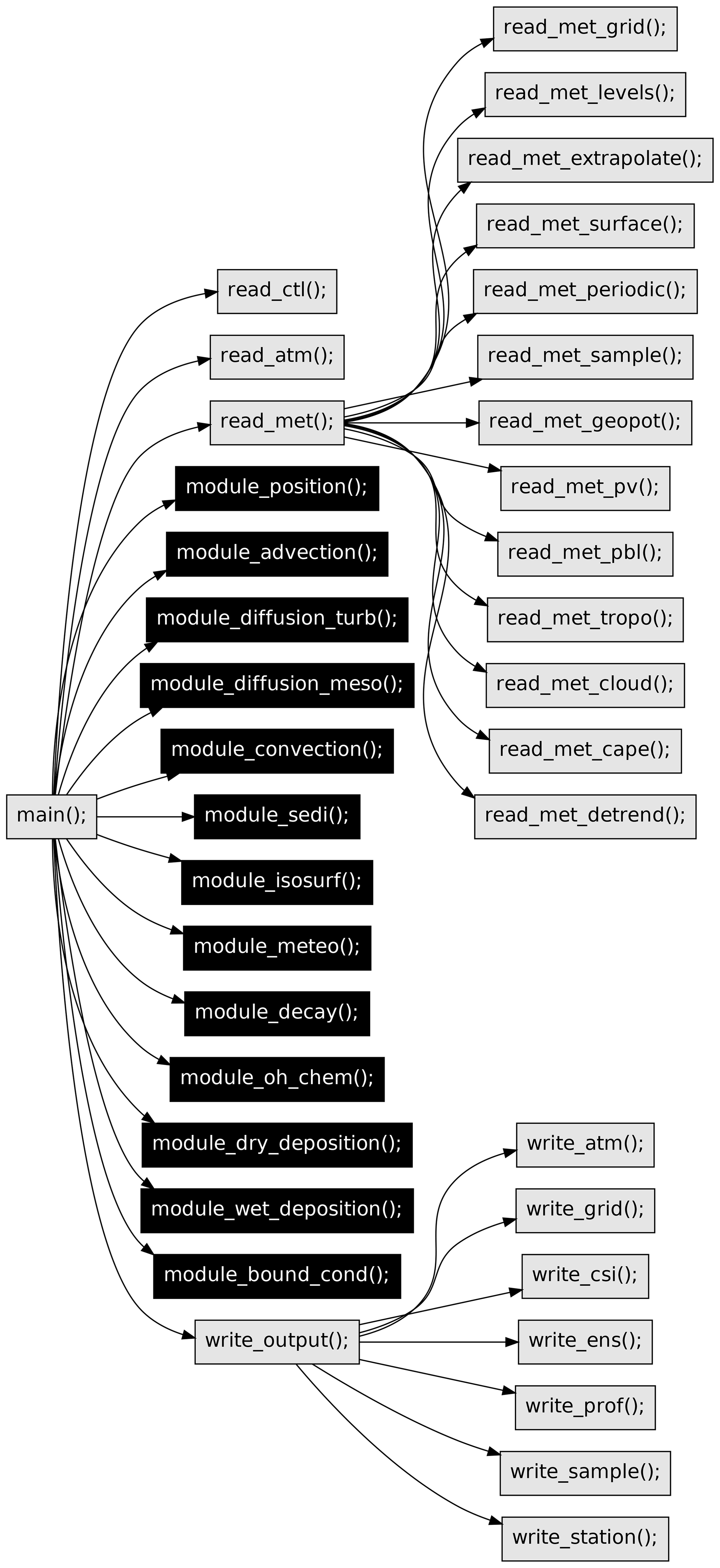
Figure 1Call graph of the most relevant functions of the MPTRAC model. The individual functions are sorted following the IPO approach; see text for details. Black boxes highlight parts of the code that are ported to GPUs.
Three main input functions are available, i.e., read_ctl to read the model control parameters, read_atm to read the initial particle data, and read_met to read the meteorological input data. The read_met function further splits into functions that deal directly with reading of the meteorological data files (read_met_grid, read_met_levels, and read_met_surface), extrapolation and sampling of the meteorological data (read_met_extrapolate, read_met_periodic, read_met_sample, and read_met_detrend), and the calculation of additional meteorological variables (read_met_geopot, read_met_pv, read_met_pbl, read_met_tropo, read_met_cloud, and read_met_cape), also referred to as meteorological data preprocessing in this work. Although the additional meteorological variables are often available directly via the meteorological input data files, the MPTRAC model allows users to recalculate these data consistently from different meteorological input data sets. The MPTRAC model input data are further discussed in Sect. 2.2.
The processing functions of MPTRAC provide the capabilities to calculate kinematic trajectories of the particles using given ω velocities (module_advection) and to add stochastic perturbations to the trajectories to simulate the effects of diffusion and subgrid-scale wind fluctuations (module_diffusion_turb and module_diffusion_meso). The functions module_convection and module_ sedi may alter the particle positions along the trajectories by simulating the effects of unresolved convection and sedimentation. The function module_isosurf allows us to vertically constrain the particle positions to different types of isosurfaces. The function module_position enforces the particle to remain within the boundaries of the model domain. The function module_meteo allows us to sample the meteorological data along the trajectories at fixed time intervals. The functions module_decay, module_oh_chem, module_dry_deposition, module_wet_deposition, and
module_bound_cond affect the mass or volume mixing ratios of the particles based on a given e-folding lifetime, chemical decomposition by the hydroxyl radical, dry and wet deposition, or by enforcing boundary conditions, respectively. Most of the chemistry and physics modules are presented in more detail in Sect. 2.3.
Finally, the model output is directed via a generic function (write_output) towards individual functions that can be used to write particle data (write_atm), gridded data (write_grid), or ensemble data for groups of particles (write_ens). The functions write_csi, write_prof, write_sample, and write_station can be used to sample the model data in specific manners to enable comparisons with observational data, such as satellite measurements or data from measurement stations. The model output is further discussed in Sect. 2.4.
All the processing functions (module_*) are highlighted in Fig. 1 to indicate that they have been ported to GPUs in the present work. Porting these processing functions to GPUs is the natural choice as these functions typically require most of the computing time, in particular for simulations with many particles. The input and output functions cannot easily be ported to GPUs as the input and output operations are directed over the CPUs and utilize CPU memory in the first place. The approach used for porting the physics and chemistry modules to GPUs and the parallelization strategy of MPTRAC are discussed in more detail in Sect. 2.5.
2.2 Model input data
2.2.1 Initial air parcel positions
In order to enable trajectory calculations, MPTRAC requires an input file providing the initial positions of the air parcels. The initial positions are defined in terms of time, log-pressure height, longitude, and latitude. Internally, MPTRAC applies pressure as its vertical coordinate. For convenience, the initial pressure p is specified in terms of a log-pressure height z obtained from the barometric formula, , with a fixed reference pressure p0=1013.25 hPa and scale height H=7 km. Longitude and latitude refer to a spherical Earth approximation, with a constant radius of curvature of RE=6367.421 km.
Internally, MPTRAC uses the time in seconds since 1 January 2000, 00:00 UTC as its time coordinate. Tools are provided along with the model to convert the internal time from and to UTC time format. The internal time step Δt of the model simulations can be adjusted via a control flag. MPTRAC allows for arbitrary start and end times of the trajectories by adjusting (shortening) the initial and the final time steps to synchronize with the internal model time steps Δt. A control flag is provided to specify whether the model should conduct the trajectory calculations forward or backward in time.
Unless the initial positions of the trajectories are derived from measurements, a set of tools provided with MPTRAC can be used to create initial air parcel files. The tool atm_init creates a regular grid of air parcel positions in time, log-pressure height, longitude, and latitude. Around each grid point and time, the tool can create random distributions of multiple particles by applying either uniform distributions with given widths or normal distributions with given standard deviations. The total mass of all air parcels can be specified, which is distributed equally over all air parcels. Alternatively, a fixed volume mixing ratio for each air parcel can be specified. With this tool, initializations for a wide range of sources (e.g., point source, vertical column, surface, or volume source) with spontaneous or continuous emissions can be created.
A tool to modify air parcel positions is atm_split. It can be used to create a larger set of air parcel positions based on randomized resampling from a given, smaller set of air parcel positions. It splits the initial small set into a larger set of air parcels. The total number of air parcels that is desired for the large set can be specified, which is helpful because it provides control over the computational time needed for a simulation. The probability by which an air parcel is selected during the resampling can be weighted by its mass. The total mass of the initial air parcels can be retained or adjusted during the resampling process. During the resampling process, uniform or Gaussian stochastic perturbations in space and time can be applied to the air parcel positions. These stochastic perturbations can be used to spread the air parcels over a larger volume, which might represent the measurement volume covered by an instrument, for example. Finally, a vertical weighting function can be applied in the resampling process in order to redistribute the air parcel positions to follow the vertical sensitivity of a satellite sounder, for instance.
2.2.2 Requirements and preprocessing of meteorological input data
Next to the particle positions, the other main input data required by MPTRAC are meteorological data from a global forecasting or reanalysis system. At a minimum, MPTRAC requires 3-D fields of temperature T, zonal wind u, and meridional wind v. The vertical velocity ω, specific humidity q, ozone mass mixing ratio , cloud liquid water content (CLWC), cloud rain water content (CRWC), cloud ice water content (CIWC), and cloud snow water content (CSWC) are optional but often needed for specific applications. The model also requires the surface pressure ps or log-surface pressure (ln ps) and the geopotential height at the surface Zg to be provided as 2-D fields. Optionally, near-surface temperature T2 m and near-surface winds (u10 m,v10 m) can be ingested from the input files.
The model requires the input data in terms of separate NetCDF files at regular time steps. The meteorological data have to be provided on a regular horizontal latitude × longitude grid. The model internally uses pressure p as its vertical coordinate; i.e., the meteorological data should be provided on pressure levels. However, the model can also ingest meteorological data on other types of vertical levels, e.g., hybrid sigma vertical coordinates η as used by ECMWF's Integrated Forecast System (IFS). In this case, the model requires p as a 3-D coordinate on the input model levels in order to facilitate vertical interpolation of the data to a given list of pressure levels for further use in the model.
Once the mandatory and optional meteorological input variables have been read in from disk, MPTRAC provides the capability to calculate additional meteorological variables from the input data. This includes the options to calculate geopotential heights, potential vorticity, the tropopause height, cloud properties such as cloud layer depth and total column cloud water, the convective available potential energy (CAPE), and the planetary boundary layer (PBL). Having the option to calculate these additional meteorological data directly in the model helps to reduce the disk space needed to save them as input data. This is particularly relevant for large input data sets such as ERA5. It is also an advantage in terms of consistency, if the same algorithms can be applied to infer the additional meteorological variables from different meteorological data sets. The algorithms and selected examples on the meteorological data preprocessing are presented in the Supplement of this paper.
2.2.3 Boundary conditions for meteorological data
The upper boundary of the model is defined by the lowest pressure level of the meteorological input data. The lower boundary of the model is defined by the 2-D surface pressure field ps at a given time. If an air parcel leaves the pressure range covered by the model during the trajectory calculations, it will be pushed back to the lower or upper boundary of the model, respectively. Therefore, the particles will follow the horizontal wind and slide along the surface or the upper boundary until they encounter an up- or downdraft, respectively. For the surface, this approach follows Draxler and Hess (1997). The next release of the MPTRAC model will provide a new option to alternatively reflect particles at the top and bottom boundaries, in order to avoid accumulation of particles at the boundaries.
We recognize that pressure might not be the best choice for the vertical coordinate of a Lagrangian model, in particular for the boundary layer, because a broad range of surface pressure variations needs to be represented appropriately by a fixed set of pressure levels. However, as the scope of MPTRAC is on applications covering the free troposphere and the stratosphere, we consider the limitation of having reduced vertical resolution in terms of pressure levels near the surface acceptable for now. The next release of MPTRAC will allow the user to choose between pressure and the isentropic-sigma hybrid coordinate (ζ) of Mahowald et al. (2002) as vertical coordinate.
For global meteorological data sets, MPTRAC applies periodic boundary conditions in longitude. During the trajectory calculations, air parcels may sometimes cross either the pole or the longitudinal boundary of the meteorological data. If an air parcel crosses the North or South Pole, its longitude will be shifted by 180∘ and the latitude will be recalculated to match the ±90∘ latitude range, accordingly. If an air parcel leaves the longitude range, it will be repositioned by a shift of 360∘ to fit the range again. The model works with both meteorological data provided at −180∘…+180∘ or 0∘… 360∘ of longitude. Following Stohl et al. (2005), we mirror data from the western boundary at the eastern boundary of the model, in order to achieve full coverage of the 360∘ longitude range and to avoid extrapolation of the meteorological input data.
2.2.4 Interpolation and sampling of meteorological data
In MPTRAC, 4-D linear interpolation is applied to sample the meteorological data at any given position and time. Although higher-order interpolation schemes may achieve better accuracy, linear interpolation is considered a standard choice in Lagrangian particle dispersion models (Bowman et al., 2013). The approach requires that two time steps of the meteorological input data are kept in memory at each time. Higher-order interpolation schemes in time would require more time steps of the input data and would therefore require more memory.
Following the memory layout of the data structures used for the meteorological input data in our code and to make efficient use of memory caches, the linear interpolations are conducted first in pressure, followed by latitude and longitude, and finally in time. Interpolations can be conducted for a single variable or all the meteorological data at once. Two separate index look-up functions are implemented for regularly gridded data (longitude and latitude) and for irregularly gridded data (pressure). Interpolation weights are kept in caches to improve efficiency of the calculations.
For various studies, it is interesting to investigate the sensitivity of the results with respect to the spatial and temporal resolution of the meteorological input data. For instance, Hoffmann et al. (2019) assessed the sensitivity of Lagrangian transport simulations for the free troposphere and stratosphere with respect to downsampled versions of the ERA5 reanalysis data set. To enable such studies, we implemented an option for spatial downsampling of the meteorological input data. The downsampling is conducted in two steps. In the first step, the full resolution data are smoothed by applying triangular filters in the respective dimensions. Smoothing of the data is required in order to avoid aliasing effects. In the second step, the data are downsampled by selecting only each th grid point in longitude, latitude, and pressure, respectively.
Note that downsampling has not been implemented rigorously for the time domain. Nevertheless, the user can specify the time interval at which the meteorological input data should be ingested. If filtering of the downsampled data is required, downsampling in time needs to be done externally by the user by applying tools such as the Climate Data Operators (CDO) (Schulzweida, 2014) to preprocess the input data of different time steps accordingly. In any case, it needs to be carefully considered whether the meteorological input data represent instantaneous or time-averaged diagnostics at the given time steps of the data.
2.3 Chemistry and physics modules
2.3.1 Advection
The advection of an air parcel, i.e., the position x(t) at time t for a given wind and velocity field v(x,t), is given by the trajectory equation,
Here, the position x is provided in a meteorological coordinate system, , with longitude λ, latitude ϕ, and pressure p. The velocity vector is composed of the zonal wind component u, the meridional wind component v, and the vertical velocity ω, respectively. Based on its accuracy and computational efficiency for trajectory calculations (Rößler et al., 2018), we apply the explicit midpoint method to solve the trajectory equation,
The model time step Δt controls the trade-off between the accuracy of the solution and the computational effort. Similar to the Courant–Friedrichs–Lewy (CFL) condition, Δt should, in general, be selected such that the steps remain smaller than the grid box size of the meteorological data. MPTRAC will issue a warning, if for a longitudinal grid spacing Δλmet of the meteorological data, the mean radius of Earth RE, and a maximum zonal wind speed, . A default time step Δt=180 s has been selected to match the effective horizontal resolution of Δx≈31 km of ECMWF's ERA5 reanalysis.
Calculations of the numerical solution of the trajectory equation require coordinate transformations between Cartesian coordinate distances and spherical coordinate distances ,
The vertical coordinate transformation between Δp and Δz uses an average scale height of H0=7 km. However, note that the vertical transformation is currently not needed to solve Eq. (2), because the vertical velocity is already provided in terms of pressure change, , in the meteorological data. The transformation is reported here for completeness, as it is required in other parts of the model. For convenience, we assume λ and ϕ to be given in radians; i.e., scaling factors of ∘ and 180∘ to convert from degrees to radians, and vice versa, do not need to be introduced here.
The coordinate transformation between Δλ and Δx in Eq. (3) bears numerical problems due to the singularities near the poles. Although this problem might be solved by means of a change to a more suitable coordinate system at high latitudes, we implemented a rather simple solution. Near the poles, for , we discard the longitudinal distance Δλ calculated from Eq. (3) and use Δλ=0 instead. The high-latitude threshold was set to ϕmax=89.999∘, a distance of about 110 m from the poles, following an assessment of its effect on trajectory calculations conducted by Rößler (2015).
As an example, Fig. 2 shows the results of kinematic trajectory calculations for particles located in the vicinity of the Northern Hemisphere subtropical jet (case A) and the Southern Hemisphere polar jet (case B) in January 2017 using ERA5 data for input. The trajectories were launched at (33.5∘ N, 165∘ W) at 11.25 km log-pressure altitude for the subtropical jet and at (57.5∘ S, 165∘ W) at 8.5 km of log-pressure altitude for the polar jet on 1 January 2017, 00:00 UTC, respectively. The trajectory seeds are located close to the horizontal wind speed maxima at 165∘ W in the upper troposphere and lower stratosphere at the given time. In both cases, the trajectories nearly circumvent the Earth during the time period of 8 d covered by the trajectory calculations. Significant horizontal meandering and height oscillations with the jet streams are revealed. The trajectories were calculated with the explicit midpoint method and a default integration time step of 180 s. Varying the time step between 45, 90, 180, 360, and 720 s did not reveal any significant deviations of the results (not shown).
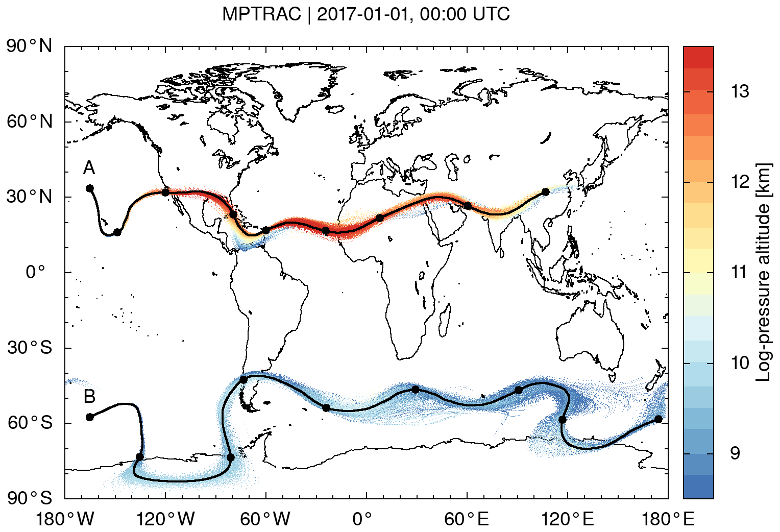
Figure 2Trajectory calculations for the Northern Hemisphere subtropical jet (case A) and the Southern Hemisphere polar jet (case B) from 1 January 2017, 00:00 UTC, to 9 January 2017, 00:00 UTC. Trajectories were launched at positions A and B at log-pressure altitudes of 11.25 and 8.5 km, respectively. Calculations used hourly ERA5 horizontal winds and vertical velocity data for input. Black curves show trajectories calculated without diffusion. Black dots indicate 24 h time intervals. Colored dots show calculations for two sets of 1000 trajectories for cases A and B with turbulent diffusion and subgrid-scale wind fluctuations being considered.
2.3.2 Turbulent diffusion
Rather complex parametrizations of atmospheric diffusivity are available for the planetary boundary layer (e.g., Draxler and Hess, 1997; Stohl et al., 2005), which have not been implemented in MPTRAC, so far. Much less is known about the diffusivities in the free troposphere and in the stratosphere, which are in the scope of our model. In MPTRAC, the effects of atmospheric diffusion are simulated by adding stochastic perturbations to the positions x of the air parcels at each time step Δt of the model,
This method requires a vector of random variates to be drawn from the standard normal distribution for each air parcel at each time step. The vector of diffusivities is composed of the horizontal diffusivity Dx and the vertical diffusivity Dz. The model allows us to specify Dx and Dz separately for the troposphere and stratosphere as control parameters. The following choices are made for the FLEXPART model (Stohl et al., 2005): default values of and Dz=0 are selected for the troposphere and Dx=0 and are selected for the stratosphere. Diffusivities will therefore change, if an air parcel intersects the tropopause. A smooth transition between tropospheric and stratospheric diffusivities is created by linear interpolation of Dx and Dz within a ±1 km log-pressure altitude range around the tropopause.
2.3.3 Subgrid-scale wind fluctuations
In addition to turbulent diffusion, the effects of unresolved subgrid-scale winds, also referred to as mesoscale wind perturbations, are considered. The starting point for this approach is the separation of the horizontal wind and vertical velocity vector v into the grid-scale mean and the subgrid-scale perturbations v′,
It is further assumed that the mean wind is given by the coarse-grid meteorological data, whereas the wind perturbations v′ need to be parameterized. The subgrid-scale wind perturbations are calculated by means of the Langevin equation,
From a mathematical point of view, this is a Markov chain or a random walk, which adds temporally correlated stochastic perturbations to the winds over time. The degree of correlation depends on the correlation coefficient r, and therefore on the time step Δt of the model and the time step Δtmet of the meteorological data. The variance (fσi)2 of the random component added at each time step depends on the grid-scale variance of the horizontal wind and vertical velocity data and a scaling factor f, which is used for downscaling to the subgrid scale. The scaling factor f needs to be specified as a control parameter of the model. The default value is f=40 %, following a choice made for the FLEXPART model (Stohl et al., 2005). For each air parcel, the grid-scale variance is calculated from the neighboring eight grid boxes and two time steps of the meteorological data. To make computations more efficient, the grid-scale variance of each parcel is kept in a cache. As before, ξ is a vector of random variates to be drawn from the standard normal distribution.
Figure 3 shows zonal means of the grid-scale standard deviations of the horizontal wind and the vertical velocity of ERA5 data for 1 January 2017. Although they are treated separately in the parametrization, we here combined the zonal and meridional wind components for convenience, noting that the standard deviations of the horizontal wind are largely dominated by the zonal wind component. The grid-scale standard deviations of the horizontal wind become as large 20 m s−1 in the tropical mesosphere. The vertical velocity standard deviations are largest (up to 0.08 m s−1) at the Northern Hemisphere midlatitude stratopause. Standard deviations are generally much lower in the troposphere and the lower stratosphere. However, some pronounced features of the horizontal wind (up to 3 m s−1) are found at the tropopause in the tropics and at northern and southern midlatitudes and for the vertical velocities (up to 0.02 m s−1) in the tropical and midlatitude upper troposphere. The parameterized subgrid-scale wind fluctuations vary significantly with time and location and the atmospheric background conditions.
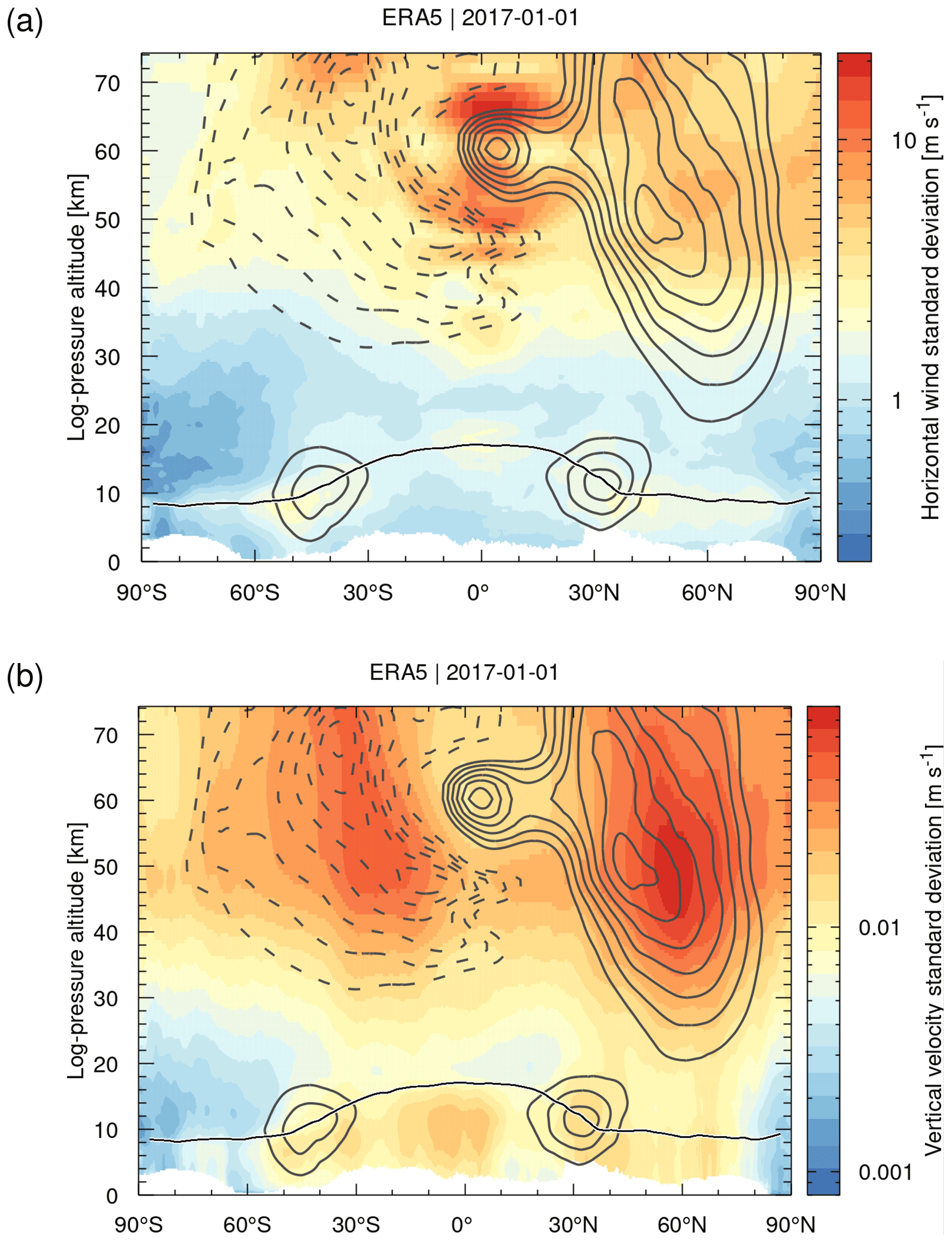
Figure 3The contour surfaces show the zonal mean standard deviations of (a) the grid-scale horizontal wind and (b) the grid-scale vertical velocity on 1 January 2017 as calculated by MPTRAC from ERA5 data. Gray curves show positive (solid) and negative (dashed) zonal mean zonal wind at levels of ±20, 30, 40, 50, 60, 70, 80 m s−1, respectively. The black curve shows the zonal mean dynamical tropopause.
Figure 2 illustrates the effects of the simulated turbulent diffusion and the subgrid-scale winds on the trajectories calculated for the jet streams. Sets of 1000 particles were released at the same starting point for both cases. The trajectory sets reveal significant horizontal and vertical spread over time. The spread mostly increases in regions where the jets are meandering and where notable horizontal and vertical wind shears are present. We calculated absolute horizontal and vertical transport deviations (AHTDs and AVTDs; see Sect. 2.4.3) in order to quantify the effects of simulated diffusion and subgrid-scale wind fluctuations on the jet stream trajectory calculations. Results for case A, the Northern Hemisphere subtropical jet, are shown in Fig. 4. The analysis of the transport deviations showed that the subgrid-scale wind fluctuations were the major source of the spread of the particles. After 8 d of trajectory time, the AHTDs and AVTDs due to the subgrid-scale winds alone (i.e., and f=40 %) were about 550 km and 450 m, respectively. In contrast, the corresponding transport deviations due to the constant diffusivities only (i.e., f=0, in the troposphere, and in the stratosphere) were about 150 km for the AHTDs and 200 m for the AVTDs.
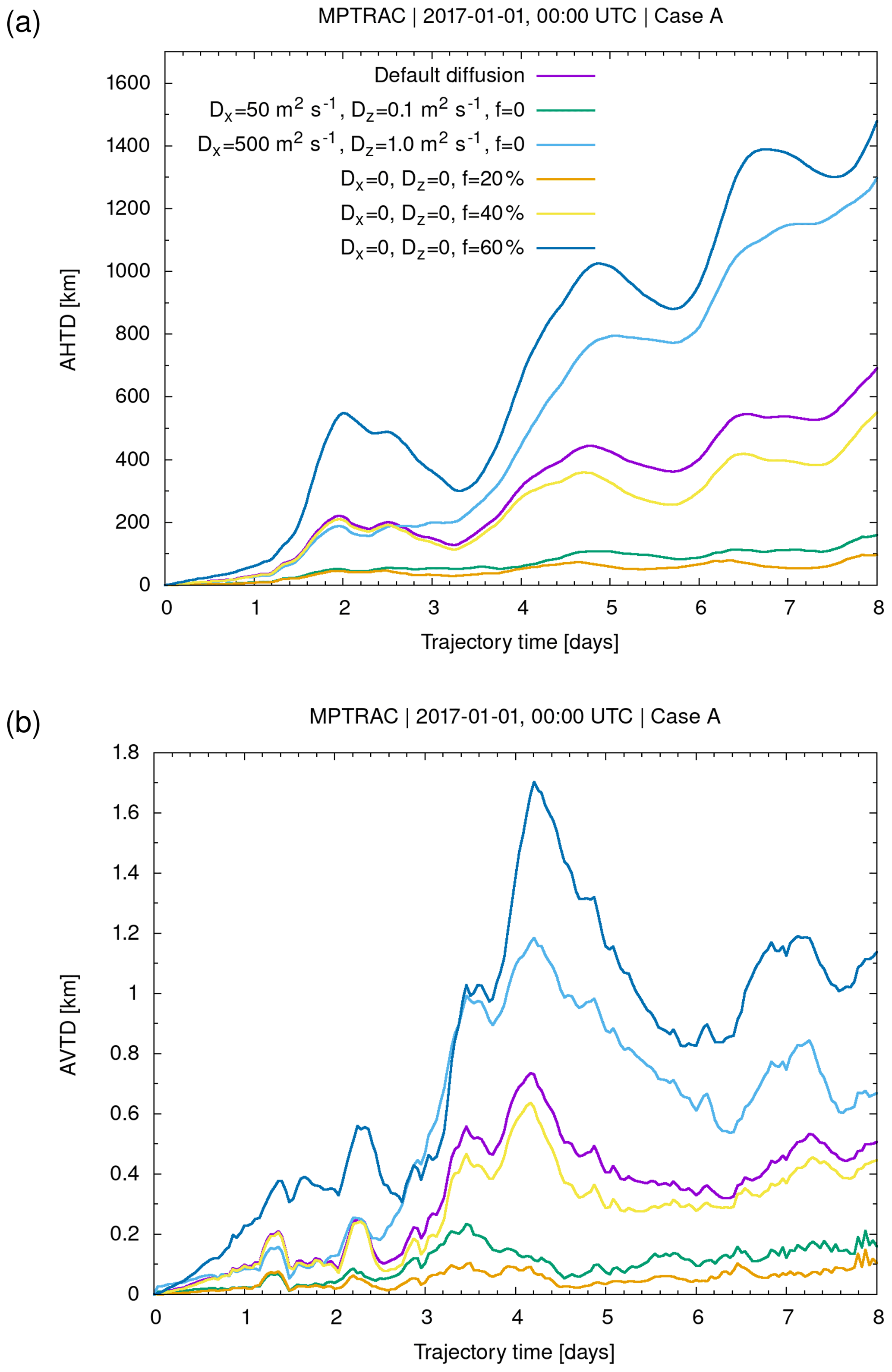
Figure 4Absolute horizontal transport deviations (AHTDs, a) and absolute vertical transport deviations (AVTDs, b) between trajectory calculations with and without simulated diffusion and subgrid-scale winds. Statistics refer to case A presented in Fig. 2. The simulations use different parameter choices of the diffusivities Dx and Dz and the scaling factor f for the subgrid-scale variances (see plot key). Default parameters (purple curve) are in the troposphere, in the stratosphere, and f=40 %.
Note that several studies with Lagrangian models provided estimates of atmospheric diffusivities (Legras et al., 2003, 2005; Pisso et al., 2009), but the data required for the free troposphere and stratosphere for the parametrizations are typically still not well constrained. In addition, in earlier work, we found that the parametrizations of diffusion and subgrid-scale winds applied here may yield different particle spread for different meteorological data sets, even if the same parameter choices are applied (Hoffmann et al., 2017). As an example, Fig. 4 shows results of sensitivity tests on the parameter choices for the diffusion and subgrid-scale wind parametrizations. The parameter choices may need careful tuning for each individual meteorological data set. However, this also opens the possibility for potentially interesting considerations regarding sensitivities to the relative importance of diffusion and subgrid wind fluctuations.
2.3.4 Convection
The spatial resolution of global meteorological input data is often too coarse to allow for explicit representation of convective up- and downdrafts. Although the downdrafts may occur on larger horizontal scales, the updrafts are usually confined to horizontal scales below a few kilometers. Furthermore, convection occurs on timescales of a few hours; i.e., hourly ERA5 data may better represent convection than 6-hourly ERA-Interim data. A parametrization to better represent unresolved convective up- and downdrafts in global simulations was implemented in MPTRAC, which is similar to the convection parametrization implemented in the Hybrid Single-Particle Lagrangian Integrated Trajectory (HYSPLIT) and Stochastic Time-Inverted Lagrangian Transport (STILT) models (Draxler and Hess, 1997; Gerbig et al., 2003). In the present study, the convection parametrization was applied for synthetic tracer simulations as discussed in Sect. 3.3.
The convection parametrization requires as input the convective available potential energy (CAPE) and the equilibrium level from the meteorological data. These data need to be interpolated to the horizontal position of each air parcel. If the interpolated CAPE value is larger than a threshold CAPE0, which is an important control parameter of the parametrization, it is assumed that the up- and downdrafts within the convective cloud are strong enough to yield a well-mixed vertical column. The parametrization will randomly redistribute the air parcels in the vertical column between the surface and the equilibrium level, which is taken as an estimate of the cloud-top height. In order to achieve a well-mixed column, the random distribution of the particles needs to be vertically weighted by air density.
The globally applied threshold CAPE0 can be set to a value near zero, implying that convection will always take place everywhere below the equilibrium level. This approach is referred to as the “extreme convection method”. It will provide an upper limit to the effects of unresolved convection. On the contrary, completely switching off the convection parametrization will provide a lower limit for the effects of unresolved convection. Intermediate states can be simulated by selecting other specific values of the threshold CAPE0, which is an important tuning parameter of the parametrization. The Supplement of this paper provides some guidance on how different choices of CAPE0 can affect the simulated convection.
The extreme convection parametrization implemented here is arguably a rather simple approach, as it relies only on CAPE and the equilibrium level from the meteorological input data. Nevertheless, first tests showed that this parametrization significantly improves transport patterns in the free troposphere. We also conducted experiments to further improve the parametrization by considering additional parameters such as the convective inhibition (CIN) to improve the onset of convection. More sophisticated convection parametrizations have been developed and implemented in Lagrangian transport models during recent years (Forster et al., 2007; Brinkop and Jöckel, 2019; Konopka et al., 2019; Wohltmann et al., 2019). These parametrizations consider additional meteorological variables such as convective mass fluxes and detrainment rates that originate from external convective parameterizations applied in state-of-the-art forecasting models. Future work may look at evaluating the extreme convection parametrization and implementing more advanced convection parametrizations in MPTRAC.
2.3.5 Sedimentation
In order to take into account the gravitational settling of particles, the sedimentation velocity vs needs to be calculated. Once vs is known, it can be used to calculate the change of the vertical position of the particles over the model time step Δt. In MPTRAC, vs is calculated for spherical particles following the method described by Jacobson (1999). In the first step, we calculate the density ρ of dry air,
from pressure p, temperature T, and the specific gas constant R of dry air. Next, the dynamic viscosity of air,
and the thermal velocity of an air molecule,
are used to calculate the mean free path of an air molecule,
as well as the Knudsen number for air,
where rp refers to the particle radius. The Cunningham slip-flow correction is calculated from
Finally, the sedimentation velocity is obtained by means of Stokes law and from the slip-flow correction,
with particle density ρp and conventional standard gravitational acceleration g. Note that rp and ρp can be specified individually for each air parcel. A larger set of parcels can be used to represent a size distribution of aerosol or cloud particles.
Figure 5 shows sedimentation velocities calculated by Eq. (16) for different particle diameters as well as pressure levels and mean temperatures at midlatitude atmospheric conditions. A standard particle density of ρp=1000 kg m−3 was considered. The sedimentation velocity vs scales nearly linearly with ρp; i.e., increasing ρp by a factor of 2 will also increase vs by the same factor. Note that the overall sensitivity on temperature T is much weaker than the sensitivity on pressure p (not shown). Sedimentation velocities are shown here up to particle Reynolds number Rep≤1, for which vs is expected to have accuracies better than 10 % (Hesketh, 1996). Larger particles will require additional corrections, which have not been implemented.
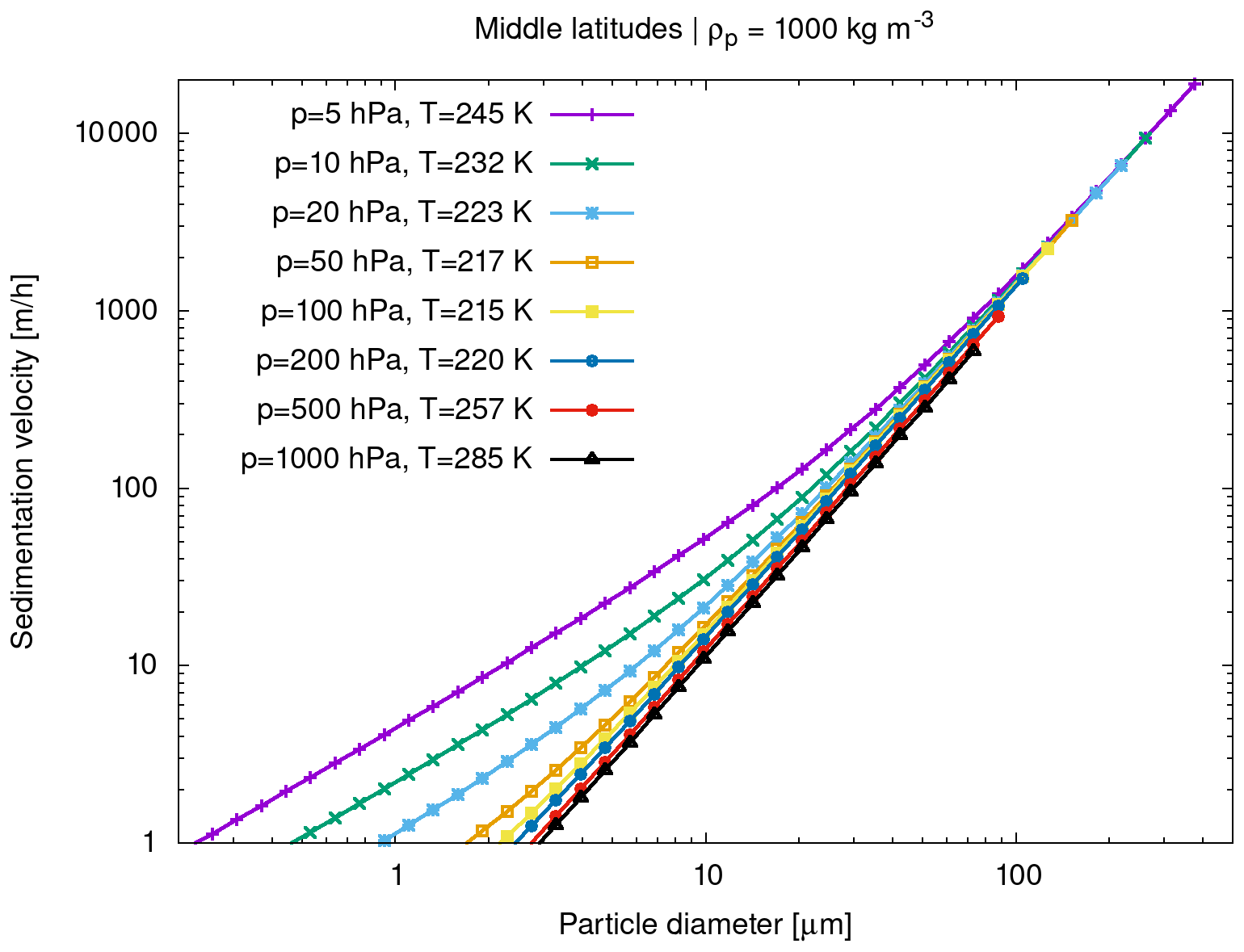
Figure 5Sedimentation velocities of spherical particles in the Stokes–Cunningham regime for different particle sizes, atmospheric pressure levels, and midlatitude mean temperatures.
2.3.6 Wet deposition
Wet deposition causes the removal of trace gases and aerosol particles from the atmosphere within or below clouds by mixing with suspended water and following washout through rain, snow, or fog. In the first step, it is determined whether an air parcel is located below a cloud top. The cloud-top pressure pct is determined from the meteorological data as the highest vertical level where cloud water or ice (i.e., CLWC, CRWC, CIWC, or CSWC) is existent. For numerical efficiency, the level pct is inferred at the time when the meteorological input data are processed. During the model run, pct can therefore be determined quickly by interpolation from the preprocessed input data. Likewise, the cloud-bottom pressure pcb is determined quickly from precalculated data.
In the second step, the wet deposition parametrization determines an estimate of the subgrid-scale precipitation rate Is, which is needed to calculate the scavenging coefficient Λ. We estimated Is (in units of mm h−1) from the total column cloud water cl (in units of kg m−2) by means of a correlation function reported by Pisso et al. (2019),
which is based on a regression analysis using existing cloud and precipitation data. At the same time as determining pct and pcb, the total column cloud water cl is calculated by vertically integrating the cloud water content data when the meteorological input data are processed. During the model run, cl can therefore also be determined quickly by horizontal interpolation of the preprocessed input data to the locations of the air parcels. For efficiency, the parametrization of wet deposition is not further evaluated for a lower limit of .
In the third step, it is inferred whether the air parcel is located within or below the cloud because scavenging coefficients will be different under these conditions. The position of the air parcel within or below the cloud is determined by interpolating the cloud water content to the position of the air parcel and by testing whether the interpolated values are larger than zero.
In the fourth step, the scavenging coefficient Λ is calculated based on the precipitation rate Is,
For aerosol particles, the constants a and b need to be specified as control parameters for the “within-cloud” and “below-cloud” cases, respectively. Typical values of and b=0.79 are used in the HYSPLIT and Next-Generation Atmospheric Dispersion Model (NAME) models (Draxler and Hess, 1997; Webster and Thomson, 2014). For gases, wet deposition depends upon their solubility and the scavenging coefficient can be calculated from
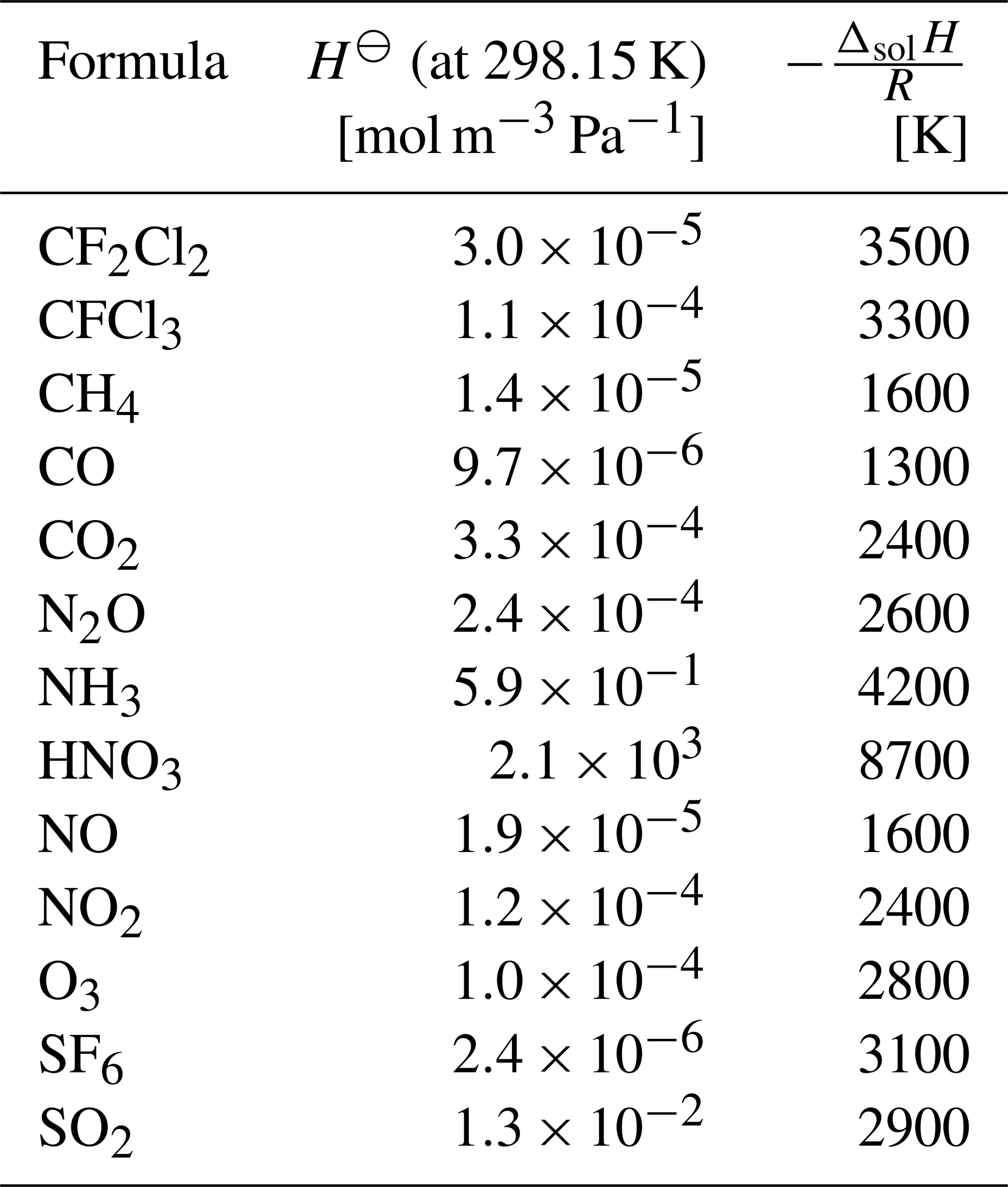
where H is Henry's law constant, R is the universal gas constant, and Δzc is the depth of the cloud layer, which we calculate from pct and pcb. Henry's law constant is obtained from
The constants H⊖ and with enthalpy of dissolution ΔsolH at the reference temperature K need to be specified as control parameters. Values for a wide range of species are tabulated by Sander (2015). The values of selected species of interest are summarized in Table 1 and included as default parameters in MPTRAC.
Finally, once the scavenging coefficient Λ for the gases or aerosol particles within or below a cloud is determined, an exponential loss of mass m over the time step Δt is calculated,
2.3.7 Dry deposition
Dry deposition leads to a loss of mass of aerosol particles or trace gases by gravitational settling or chemical and physical interactions with the surface in the dry phase. In the parametrization implemented in MPTRAC, dry deposition is calculated for air parcels located in the lowermost Δp=30 hPa layer above the surface. This corresponds to a layer width of Δz≈200 m at standard conditions.
For aerosol particles, the deposition velocity vdep will be calculated as described in Sect. 2.3.5 as a function of surface pressure p and temperature T as well as particle radius rp and particle density ρp. For trace gases, the deposition velocity vdep needs to be specified as a control parameter. Currently, this parameter is set to a constant value across the globe for each trace gas. For future applications with a stronger focus on the boundary layer, vdep will need to vary geographically to account for dependence on the surface characteristics and atmospheric conditions.
For both particles and gases, we calculated the loss of mass based on the deposition velocity vdep, the model time step Δt, and the surface layer width Δz from
Note that both the dry deposition and the wet deposition parametrization were implemented only very recently and need further testing and evaluation in future work. They will also have to be compared to more advanced parametrizations (e.g., Webster and Thomson, 2011, 2014). The parametrizations are described here for completeness, but they were not included in the model verification and performance analysis in Sect. 3.
2.3.8 Hydroxyl chemistry
In this section, we discuss the MPTRAC module that is used to simulate the loss of mass of a chemical species by means of reaction with the hydroxyl radical. The hydroxyl radical (OH) is an important oxidant in the atmosphere, causing the decomposition of many gas-phase species. The oxidation of different gas-phase species with OH can be classified into two main categories, bimolecular reactions (e.g., reactions of CH4 or NH3), and termolecular reactions (e.g., CO or SO2).
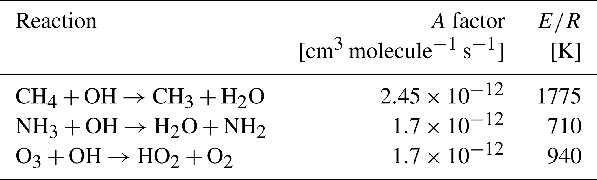
For bimolecular reactions, the rate constant is calculated from Arrhenius law,
where A refers to the Arrhenius factor, E to the activation energy, and R to the universal gas constant. For bimolecular reactions, the Arrhenius factor A and the ratio need to be specified as control parameters. The reaction rate coefficients for various gas-phase species can be found in the Jet Propulsion Laboratory (JPL) data evaluation (Burkholder et al., 2019). Table 2 lists bimolecular reaction rate coefficients for some species of interest, which were also implemented as default values directly into MPTRAC.
Table 2Bimolecular reaction rate coefficients for the hydroxyl radical. See Burkholder et al. (2019) for reference.
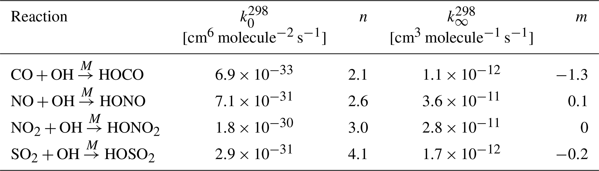
Termolecular reactions require an inert component M (e.g., N2 or O2) to stabilize the excited intermediate state. Therefore, the reaction rate shows a temperature and pressure dependence and changes smoothly between the low-pressure-limiting rate k0 and high-pressure-limiting rate k∞. Based on the molecular density of air,
with Avogadro constant NA, the effective second-order rate constant k is calculated from
The low- and high-pressure limits of the reaction rate constant are given by
The constants and at the reference temperature of 298 K and the exponents n and m need to be specified as control parameters. The exponents can be set to zero in order to neglect the temperature dependence of the low- or high-pressure limits of k0 and k∞. The termolecular reaction rate coefficients implemented directly into MPTRAC are listed in Table 3.
Table 3Termolecular reaction rate coefficients for the hydroxyl radical. See Burkholder et al. (2019) for reference.
Based on the bimolecular reaction rate k=k(T) from Eq. (23) or the termolecular reaction rate from Eq. (25), the loss of mass of the gas-phase species over time is calculated from
The hydroxyl radical concentrations [OH] are obtained by bilinear interpolation from the monthly mean zonal mean climatology of Pommrich et al. (2014). This approach is suitable for global simulations covering at least several days, as hydroxyl concentrations may vary significantly between day- and nighttime as well as the local atmospheric composition.
2.3.9 Exponential decay
A rather generic module was implemented in MPTRAC, to simulate the loss of mass of an air parcel over a model time step Δt due to any kind of exponential decay process, e.g., chemical loss or radioactivity,
The e-folding lifetime te of the species needs to be specified as a control parameter. As typical lifetimes may differ, we implemented an option to specify separate lifetimes for the troposphere and stratosphere. A smooth transition between the tropospheric and stratospheric lifetime is created within a ±1 km log-pressure altitude range around the tropopause.
2.3.10 Boundary conditions
Finally, a module was implemented to impose constant boundary conditions on particle mass or volume mixing ratio. At each time step of the model, all particles that are located within a given latitude and pressure range can be assigned a constant mass or volume mixing ratio as defined by a control parameter of the model. Next to specifying fixed pressure ranges in the free troposphere, stratosphere, or mesosphere to define the boundary conditions, it is also possible to specify a fixed pressure range with respect to the surface pressure, in order to define a near-surface layer.
The boundary condition module can be used to conduct synthetic tracer simulations. For example, the synthetic tracer E90 (Prather et al., 2011; Abalos et al., 2017) is emitted uniformly at the surface and has a constant e-folding lifetime of 90 d throughout the entire atmosphere. In our study, we implemented this by assigning a constant volume mixing ratio of 150 ppb to all air parcels residing in the lowermost 30 hPa pressure range above the surface. With its 90 d lifetime, the tracer E90 quickly becomes well mixed in the troposphere. However, the lifetime is much shorter than typical timescales of stratospheric transport. The tracer E90 therefore exhibits sharp gradients across the tropopause. Being a passive tracer in the upper troposphere and lower stratosphere region, E90 is evaluated in studies related to the chemical tropopause and stratosphere–troposphere exchange.
Another example of a synthetic tracer is ST80, which is defined by a constant volume mixing ratio of 200 ppb above 80 hPa and a uniform, fixed 25 d e-folding lifetime in the troposphere (Eyring et al., 2013). Like E90, the tracer ST80 is of interest in investigating stratosphere–troposphere exchange. The Northern Hemisphere synthetic tracer (NH50) is considered to assess interhemispheric gradients in the troposphere. It is defined by a surface layer volume mixing ratio of 100 ppb over 30 to 50∘ N and a uniform 50 d e-folding lifetime (Eyring et al., 2013). Simulation results of E90, ST80, and NH50 obtained with the CPU and GPU code of MPTRAC will be discussed in Sect. 3.3.
2.4 Model output data
2.4.1 Sampling of meteorological data
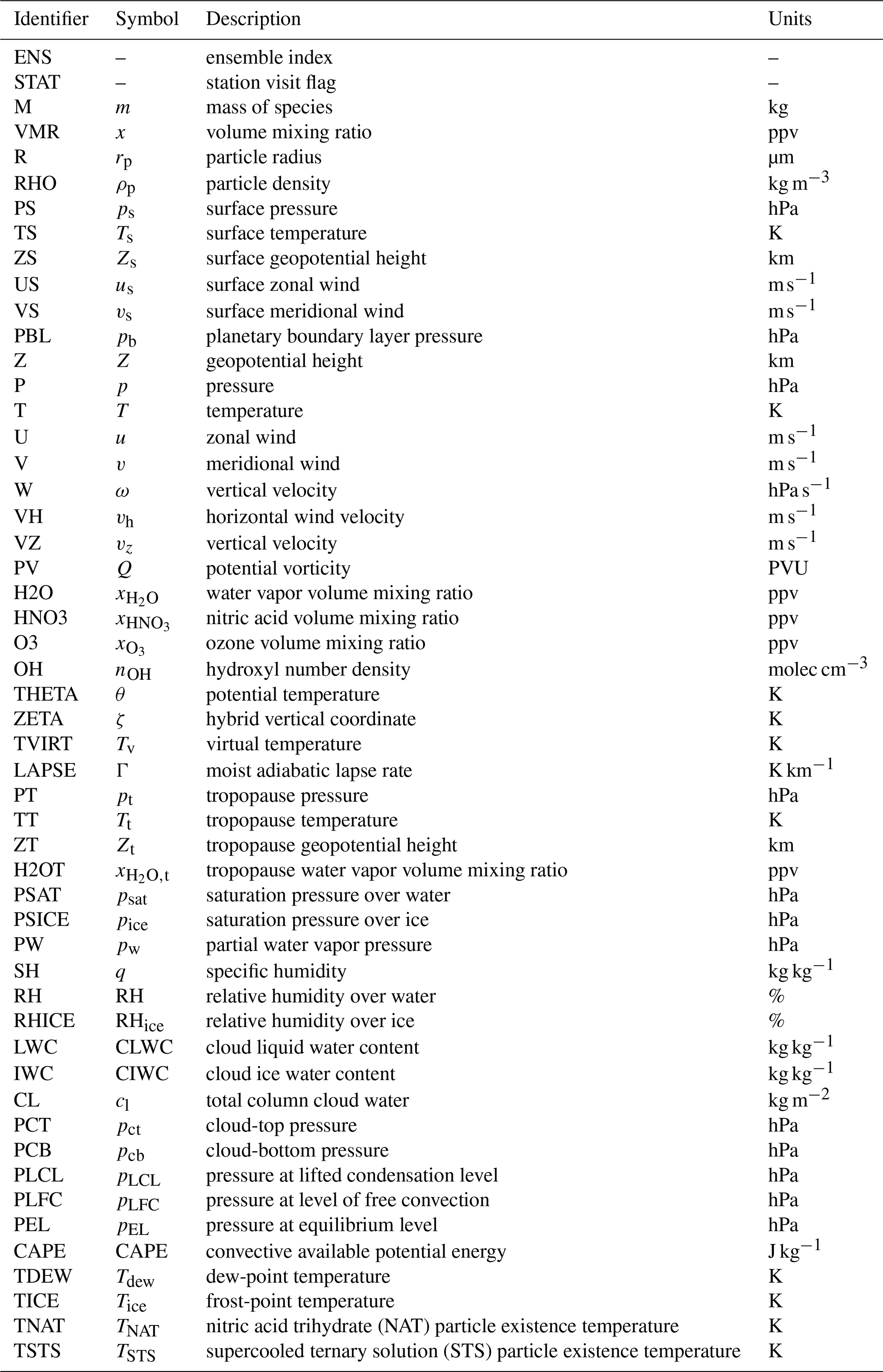
For diagnostic purposes, it is often necessary to obtain meteorological data along the trajectories. However, typically only a limited subset of the meteorological variables is of interest. Therefore, we introduced the concept of “quantities”, allowing the user to select, which variables should be calculated and stored in the output data files. Next to selecting the specific types of model output that are desired, also a list of the specific quantities that should be provided as output needs to be specified via control parameters. In total, about 50 output variables are implemented in MPTRAC (Table 4). In addition to the predefined output variables, it is possible to include user-defined variables. The user-defined variables are typically not modified during the simulations, but they are useful to store information that are required for further analyses. For example, the starting time and position of the particles can be stored as user-defined variables, and they can later be used to calculate the trajectory time or the distance from the origin.
A distinct module was implemented into MPTRAC that is used to sample the meteorological data along the trajectories. This module can become demanding in terms of computing time, as it requires the interpolation of up to 10 3-D variables and 16 2-D variables of meteorological data that are either read in from the meteorological input data files or calculated during the preprocessing of the meteorological data. However, the computing time needs of this module are typically strongly reduced by the fact that meteorological data along the trajectories are usually not required at every model time step but only at user-defined output intervals.
Next to the option of sampling of the meteorological data along the trajectories, we also implemented tools to provide direct output of the meteorological data. This includes tools to extract maps, zonal mean cross sections, and vertical profiles on pressure or isentropic levels. These tools allow for time averaging over multiple meteorological data files. Another tool is available to sample the meteorological data based on a list of given times and positions, without involving any trajectory calculations. Altogether, these tools provide a great flexibility in exploiting meteorological data in many applications.
2.4.2 Output from Lagrangian transport simulations
At present, MPTRAC offers seven output options, referred to as “atmospheric output”, “grid output”, “CSI output”, “ensemble output”, “profile output”, “sample output”, and “station output”. The most comprehensive output of MPTRAC is the atmospheric output. Atmospheric output files can be generated at user-defined time intervals, which need to be integer multiples of the model time step Δt. The atmospheric output files are the most comprehensive type of output because they contain the time, location, and the values of all user-defined quantities of each individual air parcel.
As the atmospheric output can easily become too large for further analyses, in particular if many air parcels are involved, the output of gridded data was implemented. This output will be generated by integrating over the mass of all parcels in regular longitude × latitude × log-pressure height grid boxes. From the total mass per grid box and the air density, the column density and the volume mixing ratio of the tracer are calculated. Alternatively, if the volume mixing ratio per air parcel is specified, the mean volume mixing ratio per grid box is reported. In the vertical, it is possible to select only a single layer for the grid output, in order to obtain total column data. Similarly, by selecting only one grid box in longitude, it is possible to calculate zonal means.
Another type of output that we used in several studies (Hoffmann et al., 2016; Heng et al., 2016) is the critical success index (CSI) output. This output is produced by analyzing model and observational data on a regular grid. The analysis is based on a 2×2 contingency table of model predictions and observations. Here, predictions and observations are counted as yes, if the model column density or the observed variable exceed user-defined thresholds. Otherwise, they would be counted as no. Next to the CSI, the counts allow us to calculate the probability of detection (POD) and the false alarm rate (FAR), which are additional skill scores that are often considered in model verification. More recently, the CSI output was extended to also include the equitable threat score (ETS), the linear and rank-order correlation coefficients, the bias, the root mean square (rms) difference, and the mean absolute error. A more detailed discussion of the skill scores is provided by Wilks (2011).
Another option to condense comprehensive particle data is provided by means of the ensemble output. This type of output requires a user-defined specific ensemble index value to be assigned to each air parcel. Instead of the individual air parcel data, the ensemble output will contain the mean positions as well as the means and standard deviations of the quantities selected for output for each set of air parcels having the same ensemble index. The ensemble output if of interest, if tracer dispersion from multiple point sources needs to be quantified by means of a single model run, for instance.
The profile output of MPTRAC is similar to the grid output as it creates vertical profiles from the model data on a regular longitude × latitude horizontal grid. However, the vertical profiles contain not only volume mixing ratios of the species of interest but also profiles of pressure, temperature, water vapor, and ozone as inferred from the meteorological input data. This output is compiled with the intention to be used as input for a radiative transfer model, in order to simulate satellite observations for the given model output. In combination with real satellite observations, this output can be used for model validation but also as a basis for radiance data assimilation.
The sample output of MPTRAC was implemented most recently. It allows the user to extract model information on a list of given locations and times, by calculating the column density and volume mixing ratio of all parcels located within a user-specified horizontal search radius and vertical height range. For large numbers of sampling locations and air parcels, this type of output can become rather time-consuming. It requires an efficient implementation and parallelization because it needs to be tested at each time step of the model whether an air parcel is located within a sampling volume or not. The numerical effort scales linearly with both the number of air parcels and the number of sampling volumes. The sample output was first applied in the study of Cai et al. (2021) to sample MPTRAC data directly on TROPOspheric Monitoring Instrument (TROPOMI) satellite observations.
Finally, the station output is collecting the data of air parcels that are located within a search radius around a given location (latitude, longitude). The vertical position is not considered here; i.e., the information of all air parcels within the vertical column over the station is collected. In order to avoid double counting of air parcels over multiple time steps, the quantity STAT (Table 4) has been introduced that keeps track on whether an air parcel has already been accounted for in the station output or not. We used this type of output in studies estimating volcanic emissions from satellite observations using the backward-trajectory method (Hoffmann et al., 2016; Wu et al., 2017, 2018).
By default, all output functions of MPTRAC create data files in an ASCII table format. This type of output is usually simple to understand and usable with many tools for data analysis and visualization. However, in the case of large-scale simulations, it is desirable to use more efficient file formats. Therefore, an option was implemented to write particle data to binary output files. Likewise, reading particle data from a binary file is much more efficient than from an ASCII file. The binary input and output is an efficient way to save or restore the state of the model during intermediate steps of a workflow. Another interesting option of output is to pipe the data directly from the model to a visualization tool. This will keep the output data in memory and directly forward it from MPTRAC to the visualization tool. This option has been successfully tested for the particle and the grid output in combination with the graphing utility gnuplot (Williams and Kelley, 2020).
2.4.3 Trajectory statistics
For diagnostic purposes, it is often helpful to calculate trajectory statistics. The tool atm_stat can calculate the mean, standard deviation, skewness, kurtosis, median, absolute deviation, median absolute deviation, minimum, and maximum of the positions and variables of air parcel data sets. The calculations can cover the entire set or a selection of air parcels, based on the ensemble variable or extracted by means of the tool atm_select. The tool atm_select allows the user to select air parcels based on a range of parcels, a log-pressure height × longitude × latitude box, and a search radius around a given geolocation. The trajectory statistics are calculated by applying the algorithms of the GNU Scientific Library (Gough, 2003).
The tool atm_dist allows us to calculate statistics of the deviations between two sets of trajectories. Foremost, this includes the AHTDs and AVTDs (Kuo et al., 1985; Rolph and Draxler, 1990; Stohl, 1998) over time,
Here, the horizontal distances are calculated approximately by converting the geographic longitudes and latitudes of the particles to Cartesian coordinates, and , followed by calculation of the Euclidean distance of the Cartesian coordinates. Vertical distances are calculated based on conversion of particle pressure to log-pressure altitude using the barometric formula.
Next to AHTDs and AVTDs, the tool atm_dist can calculate the relative horizontal and vertical transport deviations (RHTDs and RVTDs), which relate the absolute transport deviations to the horizontal and vertical path lengths of individual trajectories. It can also be used to quantify the mean absolute and relative deviations as well as the absolute and relative bias of meteorological variables or the relative tracer conservation errors of dynamical tracers over time. The definitions of these quantities and more detailed descriptions are provided by Hoffmann et al. (2019). In this study, we mostly present absolute transport deviations to evaluate the differences between CPU and GPU trajectory calculations (Sect. 3.2).
2.5 Parallelization strategy
Lagrangian particle dispersion models are well suited for parallel computing as large sets of air parcel trajectories can be calculated independently of each other. The workload is “embarrassingly parallel” or “perfectly parallel” as little to no effort is needed to separate the problem into a number of independent parallel computing tasks. In this section, we discuss the MPI–OpenMP–OpenACC hybrid parallelization implemented in MPTRAC. The term “hybrid parallelization” refers to the fact that several parallelization techniques are employed in a simulation at the same time.
MPI is a communication protocol and standardized interface to enable point-to-point and collective communication between computing tasks. MPI provides high performance, scalability, and portability. It is considered as a leading approach used for high-performance computing. The OpenMP application programming interface supports multi-platform shared-memory multiprocessing programming for various programming languages and computing architectures. It consists of a set of compiler directives, library routines, and environment variables that are used to distribute the workload over a set of computing threads on a compute node. An application built with an MPI–OpenMP hybrid approach can run on a compute cluster, such that OpenMP can be used to exploit the parallelism of all hardware threads within a multi-core node while MPI is used for parallelism between the nodes. Open accelerators (OpenACC) is a programming model to enable parallel programming of heterogeneous CPU–GPU systems. As in OpenMP, the source code of the program is annotated with “pragmas” to identify the areas that should be accelerated by using GPUs. In combination with MPI and OpenMP, OpenACC can be used to conduct multi-GPU simulations.
The GPU parallelization is a new feature since the release of version 2.0 of MPTRAC. Various concepts for employing GPUs are available for scientific high-performance computing. The simplest option is to replace standard computing libraries by GPU-enabled versions, which are provided by the vendors of the GPU hardware such as the NVIDIA company. A prominent example of such a library, which was ported to GPUs, is the Basic Linear Algebra Subprograms (BLAS) library for matrix–matrix, matrix–vector, and vector–vector operations. However, as MPTRAC does not employ the BLAS library, this simple parallelization technique was not considered helpful for porting our model to GPUs. At the other end of the options for GPU computing, the Compute Unified Device Architecture (CUDA) is a dedicated application programming model for GPUs. The CUDA programming model is often considered to be most flexible and allows for most detailed control over the GPU hardware. However, CUDA requires solid knowledge on GPU technology and it may cause error-prone and time-consuming work if legacy code needs to be rewritten (Li and Shih, 2018).
OpenACC can help to overcome the practical difficulties of CUDA and reduces the coding workload for developers significantly. We considered OpenACC to be a more practical choice for porting MPTRAC to GPUs as the code of the model should remain understandable and maintainable by students and domain scientists that may not be familiar with the details of more complex GPU programming concepts such as CUDA. By using OpenACC, we found that we were able to maintain the same code base of the MPTRAC model rather than having to develop a CPU and a GPU version of the model independently of each other. Next to easiness in terms of maintenance and portability of the code, the common code base is considered a significant advantage to check for bit-level agreement of CPU and GPU computations and reproducibility of simulation results.
Algorithm 1 illustrates the GPU porting of the C code of MPTRAC by means of OpenACC pragmas. Two important aspects need to be considered. First, the pragma #pragma acc parallel loop independent gang vector is used to distribute the calculations within the loops over the particles over the compute elements of the GPU device. In this example, the loop over the particles within the advection module used to calculate the trajectories is offloaded to GPUs. For compute kernels that are used inside of a GPU parallelized code block, the compiler will create both a CPU and a GPU version of the kernel. In this example, the pragma #pragma acc routine (intpol_met_time_3d) instructs the compiler to create CPU and GPU code for the function used to interpolate meteorological data, as used within and outside of the advection module. Algorithm 1 also shows that if the code is compiled without GPU support (as identified by the _OPENACC flag), the fall-back option is to apply OpenMP parallelization for the compute loops on the CPUs (#pragma omp parallel for default(shared)). The OpenMP parallelization was already implemented in an earlier, CPU-only version of MPTRAC.
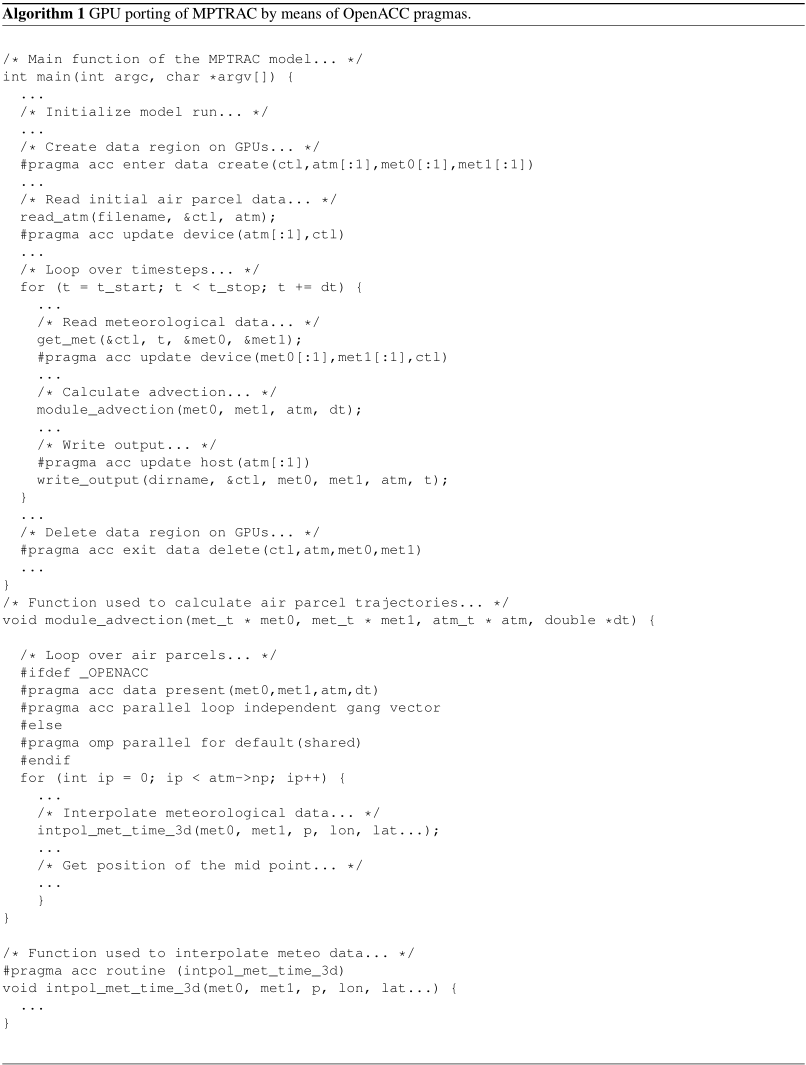
The second aspect of GPU porting by means of OpenACC is concerned with the data management. In principle, the data required for a calculation need to be copied from CPU to GPU memory before the calculation and need to be copied back from GPU to CPU memory after the computation finished. Although NVIDIA's “CUDA Unified Memory” technique makes sure, these data transfers can be done automatically, frequent data transfers can easily become a bottleneck of the code. Therefore, we implemented additional pragmas to instruct the compiler when a data transfer is actually required.
The pragma #pragma acc enter data create(ctl,atm[:1],met0[:1],met1[:1]) in Algorithm 1 creates a data region and allocates memory for the model control parameters (ctl), air parcel data (atm), and meteorological data (met0, met1) on the GPU. The data region is deleted and the GPU memory is freed by #pragma acc exit data delete(ctl,atm,met0,met1) at the end of the main function. Within the data region, the associated data will remain present in GPU memory. Within the data region, the pragma #pragma acc update device(atm[:1],ctl) is used to explicitly copy data from CPU to GPU memory, whereas #pragma acc update host(atm[:1]) is used to copy data from GPU to CPU memory. In the MPTRAC model, a single large data region was created around the main loop over the time steps of the model. As a consequence, the calls to all physics and chemistry modules will be conducted completely on GPU memory. Data transfers between CPUs and GPUs are needed only for updating of the meteorological data or for writing model output.
In total, about 60 pragmas had to be implemented in the code to parallelize the computational loops and to handle the data management to facilitate the GPU porting of MPTRAC by means of OpenACC. Code parts that were ported to GPUs are highlighted in the call graph shown in Fig. 1. Next to the OpenACC pragmas, some additional code changes were necessary to enable the GPU porting. In the original CPU code, the GNU Scientific Library (GSL) was applied to conduct a number of tasks, for instance, to compute statistics of data arrays. As the GSL is not ported to GPUs, the corresponding functions had to be rewritten without usage of the GSL. The GSL was also used to generate random numbers. Here, we implemented NVIDIA's CUDA random number generation library (cuRAND) as an efficient replacement for distributed random number generation on GPUs. Also, we found that some standard math library functions were not available with Portland Group, Inc. (PGI)'s C compiler; e.g., a replacement had to be implemented for the math function fmod used to calculate floating point modulo. For earlier versions of the PGI C compiler, we also found a severe bug when large data structures (>2 GB) were transferred from CPU to GPU memory. Nevertheless, despite a number of technical issues, we consider the porting of MPTRAC to GPUs by means of OpenACC to be straight forward and would recommend it for other applications.
3.1 Description of the GPU test system and software environment
The model verification and performance analysis described in this section was conducted on the JUWELS system (Jülich Supercomputing Centre, 2019). The JUWELS system is considered as a major target system for running Lagrangian transport simulations with MPTRAC in future work. The JUWELS system is composed of a CPU module, referred to as the JUWELS Cluster, and a GPU module, referred to as the JUWELS Booster. The JUWELS Booster and the JUWELS Cluster can be used jointly as a heterogeneous, modular supercomputer, or they can be used independently of each other. The JUWELS Booster was used as a test system in this study.
The JUWELS Booster consists of 936 compute nodes, each equipped with four NVIDIA A100 Tensor Core GPUs. Each NVIDIA A100 GPU comprises 6912 INT32 and 6912 FP32 compute cores as well as 3456 FP64 compute cores, the latter being most relevant for us because most calculations in MPTRAC are conducted at double precision. It also features 432 tensor cores, providing 8× peak speed-up for mixed-precision matrix multiplication compared to standard FP32 precision operations. The numbers of compute elements listed here indicate the large degree of parallelism required for the compute problem, which is exploited by large numbers of particles in the Lagrangian transport simulations. The A100 GPUs are equipped with 40 GB HBM2e memory per device, connected with the third-generation NVLink lossless, high-bandwidth, low-latency shared memory interconnect, providing 1555 GB s−1 of memory bandwidth. The A100 GPU supports the new Compute Capability 8.0. NVIDIA (2020) provides a detailed description of the Ampere architecture.
The JUWELS Booster GPUs are hosted by AMD EPYC Rome 7402 CPUs. Each compute node of the Booster comprises two CPU sockets, four non-uniform memory access (NUMA) domains per CPU, and six compute cores per NUMA domain, which provide two-way simultaneous multithreading. Up to 48 physical threads or 96 virtual threads can be executed on the CPUs of a compute node. The compute nodes are equipped with 512 GB DDR4-3200 RAM. They are connected by a Mellanox HDR200 InfiniBand ConnectX 6 network in a DragonFly+ topology. CPUs, GPUs, and network adapters are connected via two PCIe Gen 4 switches with 16 PCIe lanes going to each device. A 350 GB s−1 network connection IBM Spectrum Scale (GPFS) parallel file system is implemented. As of November 2020, the JUWELS Booster yields a peak performance (Rpeak) of 70.98 PFlop s−1 (see https://www.top500.org/lists/top500/2020/11/, last access: 21 May 2021).
The software environment on JUWELS is based on the CentOS 8 Linux distribution. Compute jobs are managed by the Slurm batch system with ParTec's ParaStation resource management. The JUWELS Booster software stack comprises the CUDA-aware ParTec ParaStation MPI and the NVIDIA HPC Software Development Kit (SDK), as used in this work. In particular, we used the PGI C Compiler (PGCC) version 21.5, which more recently was rebranded and integrated as NVIDIA C compiler (NVC) in NVIDIA's HPC SDK, and the GNU C compiler (GCC) version 10.3.0 to compile the GPU and CPU code, respectively. We applied the compile flag for strong optimization (-O3) for both GCC and PGCC. For other standard compile flags, please refer to the makefile in the MPTRAC code repository. MPTRAC was built with the NetCDF library version 4.7.4 and HDF5 library version 1.12.0 for file I/O. GSL version 2.7 was used for generating random numbers on the CPUs. The cuRAND library from the CUDA Toolkit release 11.0 was applied for random number generation on the GPU devices.
3.2 Comparison of kinematic trajectory calculations
In this section, we discuss comparisons of kinematic trajectory calculations conducted with the CPU and GPU versions of the MPTRAC model. For the CPU simulations, we considered binaries created with two different C compilers. The CPU code compiled with GCC is considered here as a reference, as this compiler has been used in most of the previous work and earlier studies with MPTRAC. The second version of the CPU binaries as well as the GPU binaries were compiled with PGCC, which is the recommended compiler for GPU applications on the JUWELS Booster.
We first focus on comparisons of kinematic trajectories that were calculated with horizontal wind and vertical velocity fields of the ERA5 reanalysis. The calculations were conducted without subgrid-scale wind fluctuations, turbulent diffusion, or convection, as these parametrizations rely on different random number generators implemented in the cuRAND and GSL libraries and utilize a different parallelization approach for random number generation for the CPU and GPU code, respectively. Individual trajectories calculated with these modules being activated are therefore not directly comparable to each other. They can only be compared in a statistical sense, as in Sect. 3.3.
We globally distributed the trajectory seeds in the pressure range from the surface up to 0.1 hPa (about 0–64 km of log-pressure altitude). The starting time of the trajectories was 1 January 2017, 00:00 UTC, and the calculations cover 60 d of trajectory time. To evaluate the trajectories, we calculated AHTDs, AVTDs, RHTDs, and RVTDs at 6-hourly time intervals (see Sect. 2.4.3). Considering that the trajectory errors often significantly depend on the altitude range of the atmosphere and to enable comparisons with earlier work (Rößler et al., 2018; Hoffmann et al., 2019), we calculated the transport deviations for log-pressure height ranges of 0–2 km (boundary layer), 2–8 km (lower to middle troposphere), 8–16 km (middle troposphere to lower stratosphere), 16–32 km (lower to middle stratosphere), 32–48 km (middle to upper stratosphere), and 48–64 km (mesosphere).
The absolute transport deviations between the GPU and CPU versions of MPTRAC with the GCC and PGCC compilers are shown in Fig. 6. Up to 30 d of trajectory time, the transport deviations between the different binaries and versions of the code are negligible; i.e., they are ≤1 km for the AHTDs and ≤1 m for the AVTDs at all heights. This corresponds to RHTDs and RVTDs of ≤0.01 % (not shown). The small deviations between the different binaries during the first 30 d might be attributed to different compiler settings, which enforce aggressive optimizations to achieve performance improvements coming by the price of rounding errors in the math library functions. After about 30 d, the small rounding errors further accumulate so that after 60 d, the differences between the PGCC GPU and CPU code results increase to up to 120 km (0.3 %) in the horizontal domain and about 70 m (0.4 %) in the vertical domain. The smallest transport deviations are found in the lower stratosphere (16 to 32 km of altitude), which is consistent with earlier work showing particularly low deviations for this height range due to favorable background wind and velocity conditions (Hoffmann et al., 2019).
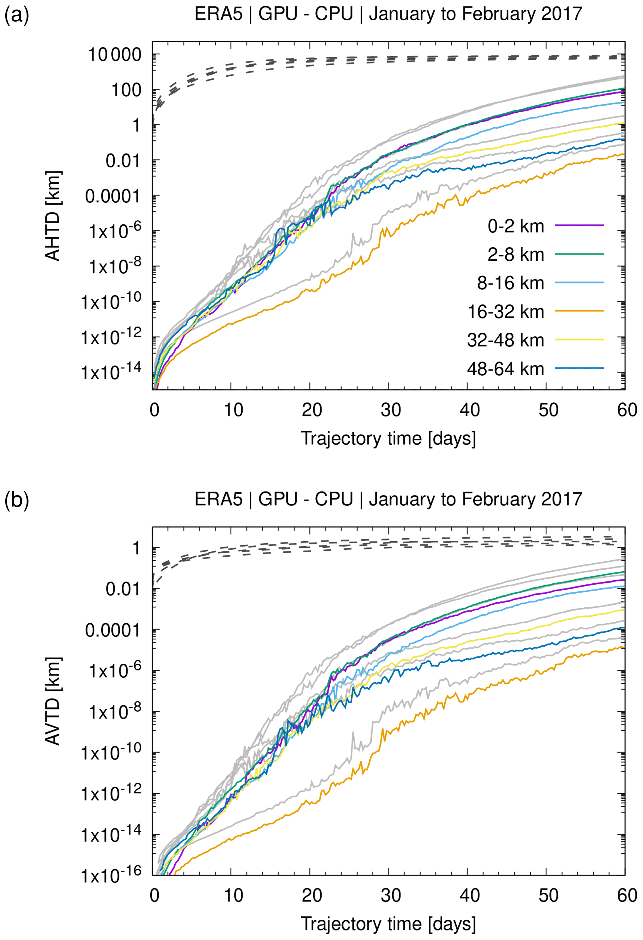
Figure 6Absolute (a) horizontal and (b) vertical transport deviations (AHTDs and AVTDs) between kinematic trajectories calculated with the CPU and GPU code of MPTRAC as compiled with the PGI C compiler (colored curves). Simulations start on 1 January 2017, 00:00 UTC and comprise 60 d of simulation time. For this test case, 106 trajectory seeds were globally distributed in different height ranges between the lower troposphere and the mesosphere (see plot key). Transport deviations between simulations using the CPU code compiled with the GNU and PGI C compilers are shown for comparison (light gray, solid curves). Transport deviations due to subgrid-scale wind fluctuations and diffusion are also shown for reference (dark gray, dashed curves).
Note that the CPU and GPU binaries created by PGCC (colored curves in Fig. 6) show somewhat better agreement (by a factor of 3 to 5) compared to deviations between the CPU binaries created by GCC and PGCC (solid gray curves). These differences between the compilers may also be attributed to different optimization settings applied at compile time. However, overall, the transport deviations found here are several orders of magnitude smaller than deviations caused by other factors, such as deviations related to different numerical integration schemes and the choice of the model time step (Rößler et al., 2018) or the impact of subgrid-scale winds and diffusion (Hoffmann et al., 2019). Therefore, we consider this result to show excellent agreement between the kinematic trajectory calculations with the GPU and CPU code and the different compilers.
3.3 Comparison of synthetic tracer simulations
With our current code, we cannot directly compare individual trajectories including the effects of turbulent diffusion and subgrid-scale winds as well as convection because these modules add stochastic perturbations to the trajectories that are created by means of the different random number generators of the cuRAND library for the GPUs and the GSL library for the CPUs. In order to compare CPU and CPU simulations considering these modules, we conducted global transport simulations of synthetic tracers with ERA5 data. In these simulations, we included the tropospheric synthetic tracers (E90 and NH50) as well as the stratospheric synthetic tracer (ST80) (Sect. 2.3.10). The simulations were initialized with 106 globally homogeneously distributed air parcels in the height range from the surface up to the lower mesosphere on 1 January 2017, 00:00 UTC. The simulations cover the entire time range of the year 2017. We assigned volume mixing ratios to the individual air parcels according to the specific initial and boundary conditions of the synthetic tracers (Sect. 2.3.10). Expecting that differences between individual trajectories are largely canceling out due to the averaging, we then compared monthly mean zonal means of the synthetic tracer volume mixing ratios from the CPU and GPU simulations.
As a representative example, Fig. 7c shows the monthly mean zonal mean distribution of E90 in July 2017 from our ERA5 simulations with the GPU code of MPTRAC. Following a spin-up time of half a year, i.e., about twice the lifetime of the E90 tracer, it is found that E90 is well mixed and rather homogeneously distributed throughout the troposphere. The 90 ppbv contour of the E90 tracer is expected to indicate the chemical tropopause (Prather et al., 2011). For our simulations, we found that the 90 ppbv contour line of E90 agrees well with the monthly mean zonal dynamical tropopause. The E90 distribution in Fig. 7c qualitatively compares well with the climatological mean presented by Abalos et al. (2017).

Figure 7Monthly mean zonal means of the synthetic tracers ST80, E90, and NH50 in July 2017 from GPU calculations (a, c, e) as well as corresponding differences between GPU and CPU simulations (b, d, f). Simulations were initialized on 1 January 2017, 00:00 UTC, with 106 homogeneously distributed trajectory seeds in the troposphere and stratosphere and are based on ERA5 meteorological input data. The synthetic tracer data are sampled on 3∘ latitude and 500 m altitude bins. The black curve shows the monthly mean zonal mean dynamical tropopause.
Figure 7d shows the differences of the E90 monthly mean zonal means between the GPU and CPU code. Despite the fact that even without diffusion or convection being considered, individual CPU and GPU trajectories already differ significantly after 60 d (Sect. 3.2), the E90 monthly mean zonal means of the CPU and GPU code agree quite well. The differences of the means are typically below ±8 ppb, which is about 5 % of the maximum volume mixing ratio of the E90 tracer. The largest differences between the CPU and GPU simulations are found near the tropopause. This region is most sensitive to statistical effects, as the tracer gradients are largest in this region. However, no systematic bias between the E90 distributions of the CPU and GPU code was revealed. The remaining differences are attributed to statistical noise, as can be seen by running simulations with different random seeds. Overall, this comparison of the E90 simulations shows good agreement between the GPU and CPU simulations.
Figure 7a and b show the July 2017 simulation results for the stratospheric synthetic tracer (ST80). Figure 7e and f show the simulation results for the Northern Hemisphere tracer (NH50). Similar to E90, the comparisons for ST80 and NH50 show that individual differences between the monthly mean zonal means from the CPU and GPU simulations are mostly below ±5 % of the maximum volume mixing ratios and that the largest differences are found in regions where sharp gradients are present in the tracer fields. Recognizing the effects of the spin-up time of the simulations and that stratospheric transport has much longer timescales than tropospheric transport, which causes some latency in particular for ST80, similar results are also found for the other months of the year 2017.
3.4 OpenMP scaling analysis
Some parts of the MPTRAC code cannot or have not been ported to GPUs. This includes the file input and output operations, which are directed via the hosting CPUs and the CPU memory, and the functions that are used for preprocessing of the meteorological data, such as the codes to calculate geopotential heights, potential vorticity, convective available potential energy, the planetary boundary layer, the tropopause height, and others. For those parts of the MPTRAC code that have not been ported to GPUs, it is important to study the OpenMP scalability on the host devices. In particular, good OpenMP scaling up to 12 threads on the JUWELS Booster needs to be demonstrated, as this is the fraction of physical cores shared by each GPU device on a JUWELS compute node.
Here, we focus on an OpenMP strong scaling test conducted by means of binaries compiled with the PGI compiler, as this is the recommended compiler for GPU applications on JUWELS Booster. For this test, the OpenMP static scheduling strategy was applied. The pinning of the threads to the CPU cores was optimized compared to the default settings of the system by using a fixed assignment of the threads to the sockets of the nodes (by setting the environment variables OMP_PROC_BIND = true and OMP_PLACES = sockets, respectively). We measured the runtime and speed-up for different numbers of OpenMP threads for a fixed set of 106 globally distributed particles for 24 h of simulation time starting 1 January 2017, 00:00 UTC. The trajectory seeds for this test are the same as those used for comparing the kinematic trajectory calculations in Sect. 3.2. However, similar to the synthetic tracer simulations described in Sect. 3.3, we not only calculated kinematic trajectories but also included the effects of turbulent diffusion and subgrid-scale wind fluctuations as well as convection in these calculations.
The results of the OpenMP strong scaling test are shown in Fig. 8. The runtimes indicate that the calculations in the physics modules (trajectories, diffusion, convection, etc.) and the meteorological data processing yield the major contributions to total runtime up to 12 OpenMP threads. At larger numbers of threads, the file input becomes the leading contribution to the total runtime. Concerning the GPU simulations, the OpenMP scaling of the meteorological data processing on the CPUs is of interest, as this is the leading component in the calculations that was not ported to GPUs. In contrast, the scaling of the physics calculations can be ignored here for now, as these calculations were ported to GPUs. For the meteorological data processing, OpenMP provides a speed-up of 10.7 (a parallel efficiency of 90 %) up to 12 threads and 20.2 (84 %) up to 24 threads (Fig. 8b). If the simulations cover more than one socket (48 threads), the parallel efficiency drops to 65 %. Enabling simultaneous multithreading (SMT) provides a further improvement of the speed-up from 31.3 at 48 threads to 37.2 at 96 threads. The OpenMP scaling of the meteorological data processing is particularly efficient compared to other parts of the code. This might be related to the fact that we selected a rather suitable memory layout for the meteorological data. Vertical columns of the meteorological data are ordered sequentially in memory, which allows for efficient use of memory caches as the preprocessing of the meteorological data is mostly conducted on vertical columns of the data.
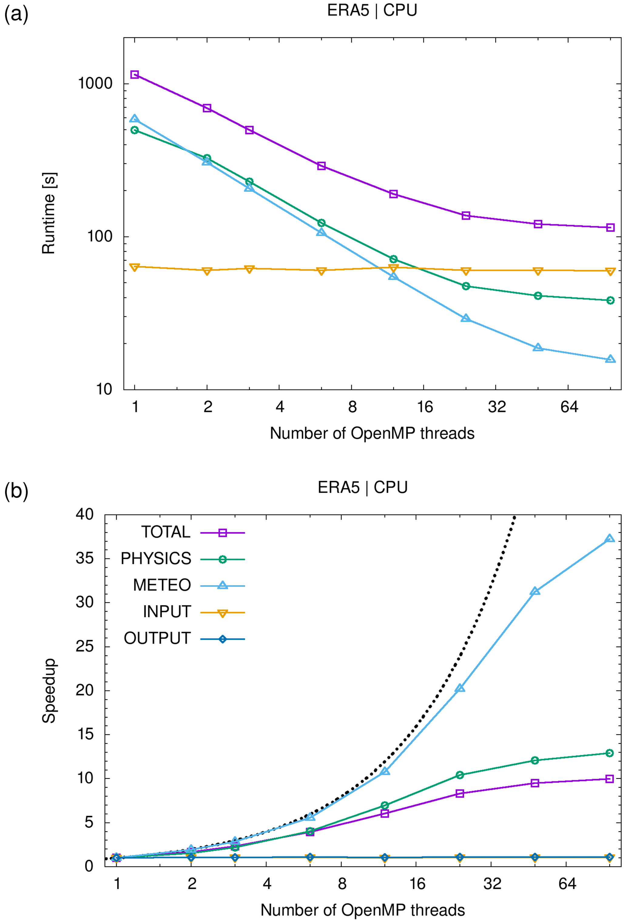
Figure 8Runtime (a) and speed-up (b) of an OpenMP strong scaling test for MPTRAC simulations on JUWELS Booster CPUs. The simulations cover a 24 h time period starting on 1 January 2017, 00:00 UTC and use ERA5 input data. The simulations were initialized with a fixed number of 106 particles with homogeneously distributed trajectory seeds. Colored curves show the OpenMP scaling for different parts of the code (see text for details). The dotted black curve indicates linear speed-up.
3.5 GPU scaling analysis
In this section, we discuss the GPU scaling of MPTRAC simulations conducted on JUWELS Booster nodes with respect to the problem size, i.e., the number of particles or trajectories that are calculated. The analysis of the scaling behavior with respect to the problem size is of interest because the NVIDIA A100 GPUs provide a particularly large number of parallel compute elements (Sect. 3.1), which require a high degree of parallelism of the problem in order fully exploit the GPU computing capacities. Here, we tested problem sizes of 100 to 108 particles in the simulations. We measured the runtime for simulations starting on 1 January 2017, 00:00 UTC, covering 24 h of simulation time. The simulations were driven by hourly ERA5 input data. Particle and grid output were written every 6 h.
Figure 9a shows the runtime of the MPTRAC simulations required for different numbers of particles on the JUWELS Booster A100 GPU devices. The scaling analysis shows that the total runtime required for the simulations is rather constant and in the range of 122 to 127 s between 100 to 106 particles. For larger numbers of particles, linear scaling is observed. The total runtime increases up to 153 s for 107 particles and 409 s for 108 particles.

Figure 9Scaling analysis showing (a) the runtime of MPTRAC simulations with respect to the number of particles on a JUWELS Booster GPU node and (b) the speed-up of GPU over CPU-only calculations. The simulations cover a 24 h time period starting on 1 January 2017, 00:00 UTC and used ERA5 input data. Colored curves in panel (a) refer to different parts of the code (see plot key). The speed-up of GPUs over CPUs shown in panel (b) was calculated for simulations with and without using NVIDIA's Unified Memory capability.
The analysis of individual contributions shows that reading of the ERA5 input data (60 to 64 s, referred to as INPUT in Fig. 9a) and preprocessing of the meteorological data (60 to 62 s, referred to as METEO) accounts for most of the total runtime for ≤107 particles. The runtime for this part of the code depends on the size of the meteorological input data and is independent of the number of particles. The computing time required to calculate the trajectories, diffusion, convection, and the decay of particle mass (referred to as PHYSICS) is rather constant (0.1 to 0.4 s) for ≤104 particles, followed by linear scaling for larger numbers of particles. A transition from constant to linear scaling in the range of 103 to 104 particles can be expected, as at least 3456 particles must be simulated at once, in order to fully exploit the A100 parallel compute capacities (Sect. 3.1). For smaller numbers of particles, a fraction of the compute elements of the GPU device remains unused. Beyond 3×10⁷ particles, the runtime required for the physics calculations exceeds the runtime required for file input and meteorological data preprocessing. The runtime for file output can be neglected in the current setup.
The same scaling test was used to estimate the speed-up achieved by applying the GPU device over a simulation that was conducted on CPUs only. Note that defining a GPU-over-CPU speed-up is a difficult task, in general, as the results will depend not only on the GPU device but also on the individual compute capacities of both the CPU and GPU devices. Nevertheless, to estimate this speed-up, we conducted corresponding CPU-only simulations and runtime measurements by applying 12 cores of a JUWELS Booster compute node. A number of 12 cores was chosen here, as this corresponds to the number of physical cores sharing a GPU device on a booster node. We think that this specific approach of estimating the GPU-over-CPU speed-up provides a fair and more realistic comparison in contrast to comparing the GPU compute capacity to just a single CPU core, for example.
The estimated speed-up due to applying the GPU devices of a JUWELS Booster compute node is shown in Fig. 9b. In the case of not using the “managed memory” option (also referred to as NVIDIA Unified Memory), which corresponds to the results shown earlier, we found a GPU-over-CPU speed-up of less than 1 for ≤105 particles; i.e., the GPU simulations are actually slower than the CPU-only simulations. This behavior changes starting from about 106 particles, with an actual speed-up of about 1.5 for 106 particles and about 5.3 for 107 particles. The GPU-over-CPU speed-up finally saturates near 16.4 for 108 particles. At these particle numbers, the speed-up of the total runtime is largely determined by the scaling for the physics calculations. Additionally, we tested NVIDIA's Unified Memory capability, which allows the programmer to avoid specifying explicit data transfers between the host and the device, by triggering those data transfers automatically, if memory cache misses occur. It is convenient not having to specify the data transfers explicitly in the code, but our tests showed that the managed memory option causes a performance degradation of about 20 % in the GPU-over-CPU speed-up.
Finally, we conducted a more detailed runtime profile analysis of the GPU simulations based on about 40 individual timers, which are implemented directly into the code. Table 5 shows the results of the profile analysis for the largest GPU simulation conducted here, covering 108 particles. This is the most compute-intensive simulation, in which about 67 % of the computing time are spent in the physics modules of MPTRAC. The calculation of the trajectories (referred to as MODULE_ADVECTION in Table 5) require about 47 % of the runtime. Adding stochastic perturbations to the trajectories to represent diffusion and subgrid-scale wind fluctuations requires 3 % and 7 % of the runtime, respectively. Simulating convection and enforcing particles to remain within the model domain both require about 3 %–4 % of the runtime.
Table 5Runtime profile of an MPTRAC simulation using ERA5 input data with 108 particles for 24 h simulation time. Runtime measurements were conducted on a JUWELS Booster GPU node. Timers with less than 0.01 s are not shown.
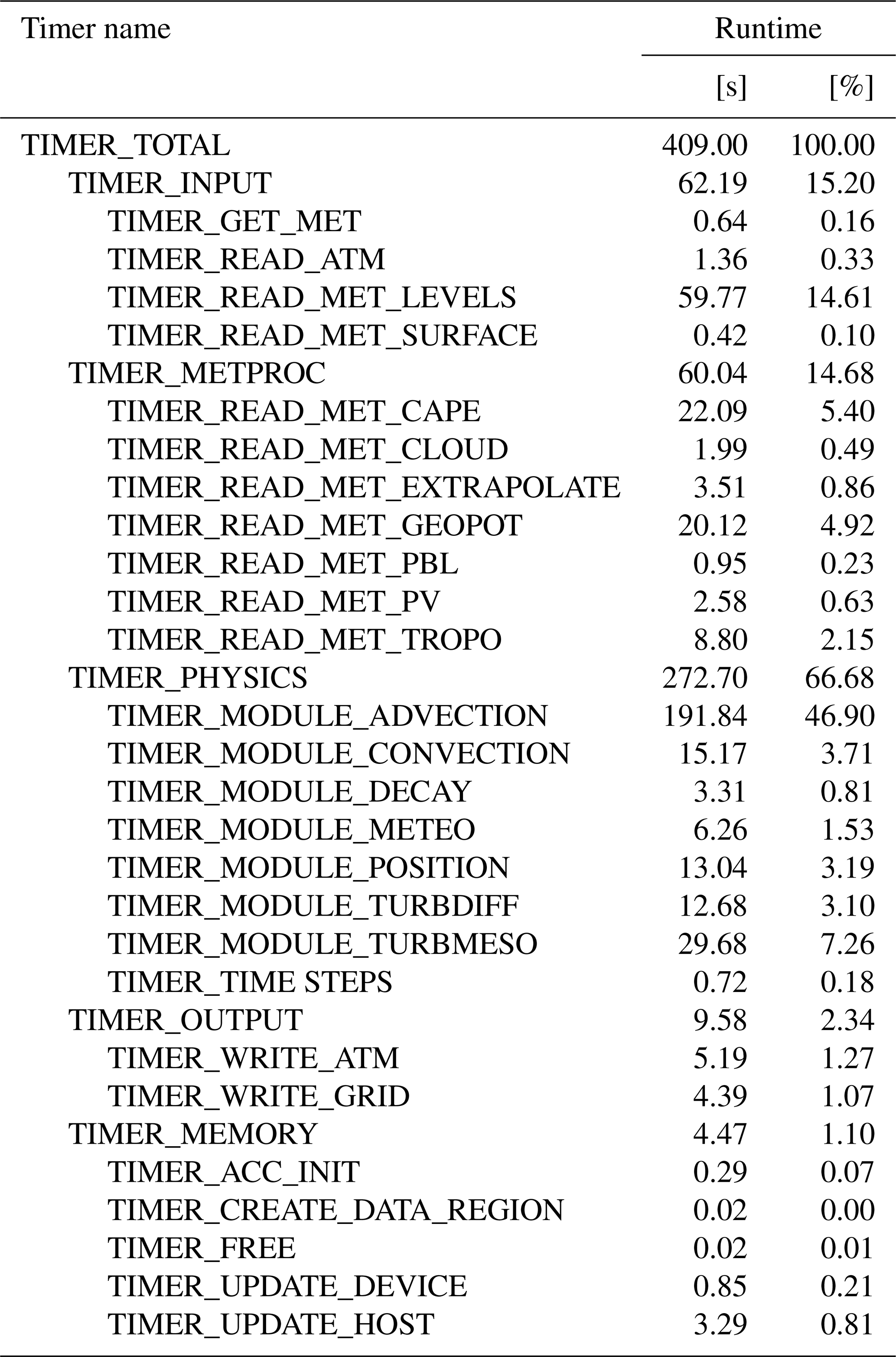
Next to the physics modules, other parts of the code required about 33 % of the overall runtime of this large-scale simulation. Reading the input data required about 15 % of the runtime, where most time was needed to read the 3-D level data of the meteorological input data. A similar amount of time (about 15 %) was required for the processing of the meteorological data, with most time spent on calculating CAPE (5.4 %), geopotential heights (4.9 %), and the tropopause (2.1 %). The runtime required for output was 2.4 % in this simulation. However, it needs to be considered that output was written only 6-hourly here. The runtime required for output would scale accordingly for more frequent output. The runtime required for data transfers between GPU and CPU memory was also about 1 %, with most time spent on transferring the input meteorological data from CPU to GPU memory. Although this profile analysis did not reveal any major bottlenecks, there is room for further improving the code of MPTRAC. Most attention should be devoted to further optimizing the advection module, as it requires most of the runtime for large-scale simulations.
3.6 Timeline analysis of GPU simulations
For a more detailed analysis of the large-scale MPTRAC simulation comprising 108 particles as discussed in Sect. 3.5, we analyzed the timeline of the simulation generated with the NVIDIA Nsight Systems performance analysis tool. Figure 10a shows the timeline for the entire 24 h simulation time period, completed in a runtime of 460 s. Note that the runtime of the Nsight Systems run comprises an overhead of about 50 s compared to the corresponding runtime profile presented in Sect. 3.5. Figure 10b shows a zoom of the timeline for about 18 s of runtime, which comprises the simulation time period in between two time steps of the ERA5 data.
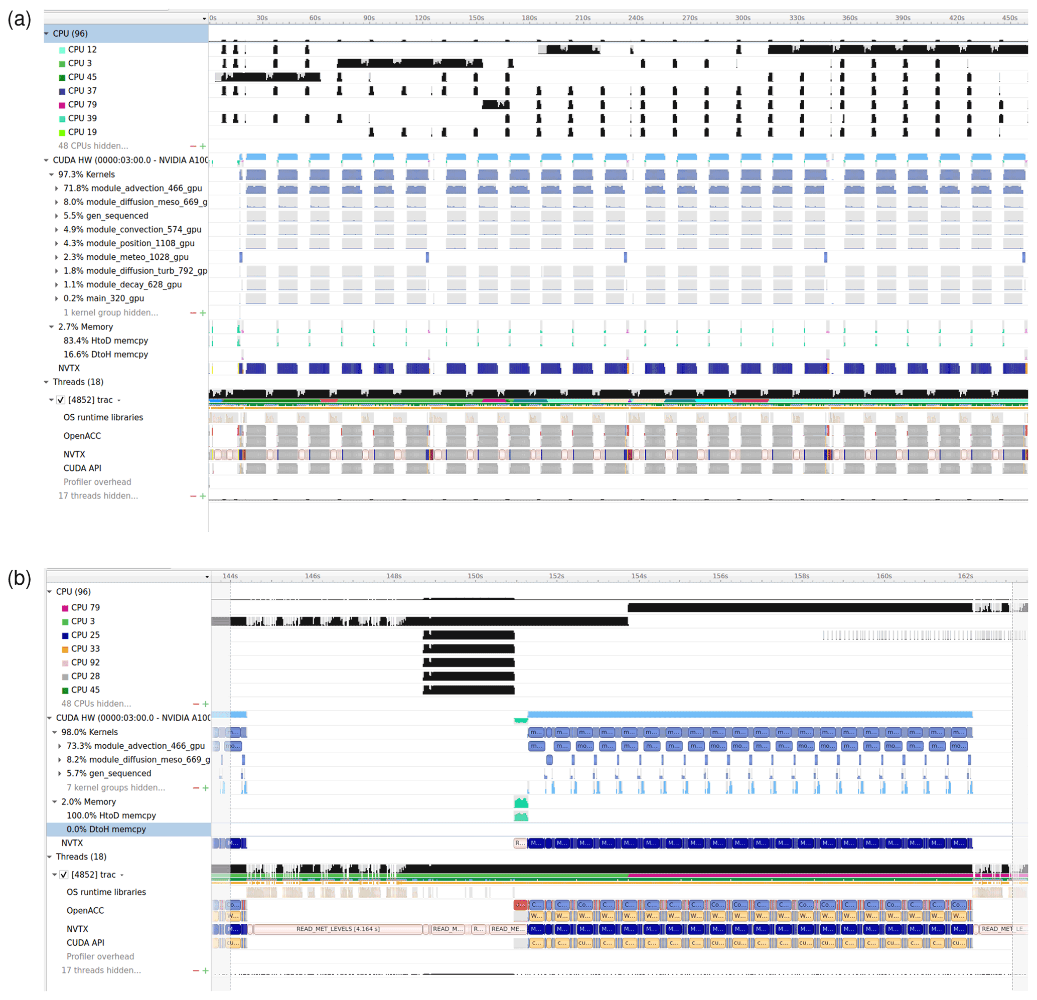
Figure 10Timeline analysis of a 24 h MPTRAC simulation comprising 108 particles driven by the ERA5 reanalysis for 1 January 2017. As an example, screenshots from the NVIDIA Nsight Systems performance analysis tool show the timeline for (a) the entire simulation and (b) a zoom for 1 h simulation time (in between two time steps of the ERA5 input data). The performance data presented here are made available via an open data repository (Haghighi Mood and Hoffmann, 2022). See text for details.
The black bars on top of Fig. 10a and b show the CPU utilization of a selected subset of the 96 virtual threads operating on a JUWELS compute node. The analysis of the CPU utilization shows that a single CPU, the master thread, is utilized during most of the runtime, i.e., to conduct computation, file I/O, or data transfers with the GPU, whereas the remaining 11 threads assigned to a GPU device are utilized via OpenMP only when the meteorological data preprocessing is conducted.
The blue bars in the middle of Fig. 10a and b indicate the GPU utilization over time. In agreement with Sect. 3.5, the timeline analysis shows regular patterns over time, where in each block about 30 % of the runtime was spent on file I/O and meteorological data preprocessing whereas about 70 % of the runtime was used for the physics calculations on the GPUs. On the GPU devices, the timeline analysis shows that 97.3 % of the time was spent in the compute kernels whereas 2.7 % of the time was required for memory transfers. For the data transfers, most of the time (83.4 %) was spent on host-to-device transfers of the ERA5 data.
The colored bars at the bottom of Fig. 10a and b provide information for the NVIDIA Tools Extension (NVTX) markers, which were inserted directly into the MPTRAC model to indicate distinct sections of the code for profiling. The bars near the bottom also provide access to profiling information on the operating system (OS) runtime libraries (which are utilized for file I/O, for instance) as well as the OpenACC and CUDA application programming interfaces.
Overall, the timeline analysis indicates that the code is providing a high utilization rate of the GPU devices, which is a basic requirement for using the GPU devices efficiently. However, the timeline analysis also reveals optimization opportunities. Overlapping file I/O and GPU computations can hide the file I/O costs with the expense of a slight increase in memory usage and reduce the wall-clock time significantly. As the meteorological data are finally required on the GPU devices to conduct the Lagrangian transport simulations, it could also be beneficial to port the meteorological data processing from the CPU to the GPU devices to accelerate the processing.
Finally, a more detailed inspection of the physics calculations on the GPUs shows that about 70 % of the time is spent in the advection module, which is used to solve the trajectory equation. A more detailed analysis indicates that this part of the code is memory bound; i.e., the runtime is limited by the GPU's global memory bandwidth. Future work should focus on optimizing this specific bottleneck of the GPU code by improving data locality and memory access patterns on the GPU devices.
3.7 Multi-GPU usage and MPI scaling test
MPTRAC provides a hybrid MPI–OpenMP–OpenACC parallelization to fully exploit the compute capacities of the JUWELS Booster. Each compute node of the booster is equipped with four NVIDIA A100 Tensor Core GPU devices. In order to utilize the capacities of the compute nodes, a multi-GPU approach is required. In MPTRAC, multiple GPU devices can be utilized by means of the MPI parallelization. With the current approach, each MPI task is assigned a single GPU device to offload computations; i.e., four MPI tasks will be operating on each compute node in the multi-GPU mode. At the same time, each MPI task can access up to 12 physical CPU cores of each node by means of the OpenMP parallelization. This scheme is particularly suited for ensemble simulations, i.e., to run many distinct MPTRAC simulations as parallel MPI tasks.
Liu et al. (2020) demonstrated good strong and excellent weak scaling of the MPI–OpenMP hybrid parallelization of MPTRAC in an inverse modeling approach for up to 38 400 computing processes on the Tianhe-2 supercomputer at the National Supercomputer Center in Guangzhou, China. Here, strong scaling is defined as how the runtime varies with the number of compute elements for a fixed total problem size. Weak scaling is defined as how the runtime varies with the number of compute elements for a fixed problem size per compute element. As the MPI approach of MPTRAC is embarrassingly parallel and does not require any communication between the MPI tasks, performance degradation is generally not expected to be related to computation or communication but might arise from other limiting factors, such as file I/O.
Figure 11 shows the results of an MPI weak scaling test on the JUWELS Booster, utilizing the MPI–OpenMP–OpenACC hybrid parallelization. Here, the test setup was slightly modified compared to earlier work. We conducted the simulations with 5×10⁷ particles. This number of particles was chosen to achieve similar fractions of runtime required for file I/O, meteorological data preprocessing, and the physics calculations. File I/O was given a significant fraction of the total runtime in this experiment (at least 25 %), as we expected this part to be most sensitive to performance degradation in the MPI scaling test. The simulation time was reduced from 24 to 6 h, to limit the overall consumption of computing resources. During the 6 h simulation time, ERA5 data for seven synoptic time steps were read from the global file system. Particle data and grid output were written once at the end of the 6 h time interval.
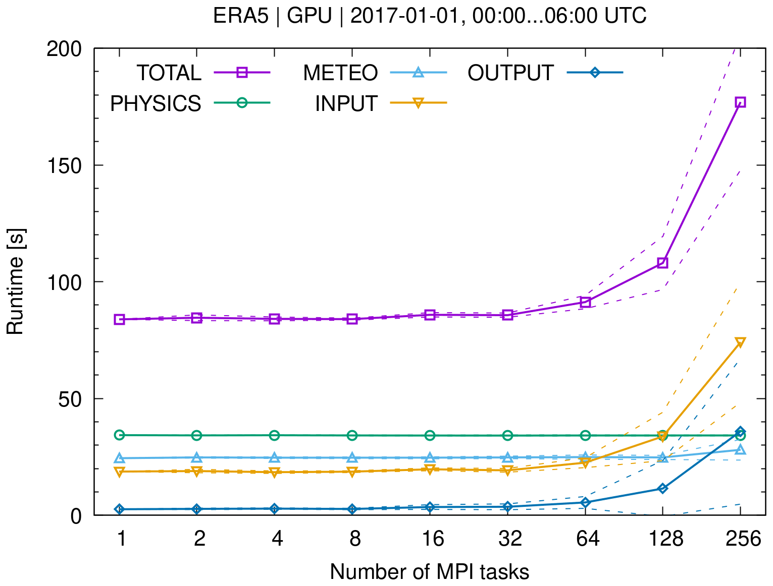
Figure 11MPI weak scaling test for MPTRAC simulations on the JUWELS Booster compute nodes. Each task utilized one GPU device and shared 12 CPU cores. The simulations cover a 6 h time period starting on 1 January 2017, 00:00 UTC and used ERA5 input data. The simulations were initialized with a fixed number of 5×10⁷ particles with homogeneously distributed trajectory seeds. Colored curves show the means (solid) and standard deviations (dashed) of the runtime for different parts of the code.
We measured the total runtime as well as the runtime for the physics calculations, meteorological data processing, file input, and file output for each MPI task. Figure 11 shows the means and standard deviations of the runtime between 1 and 256 MPI tasks. The scaling test shows that the runtime for the meteorological data preprocessing and physics calculations is rather constant over the complete range of MPI tasks tested here. The runtime for file I/O is nearly constant up to 64 MPI tasks, whereas it significantly increases and shows larger fluctuations for 128 and 256 MPI tasks. Such limitations and fluctuations in runtime for file I/O are expected because the global file system of the JUWELS Booster is a shared resource and increasing data volumes from our own simulations as well as processes from other users of the system might have affected the runs while the scaling tests were conducted. The MPI scaling test indicates reasonable scaling up to 256 MPI tasks, but it also shows that file I/O will become a bottleneck for larger simulations, at least if large-scale data sets, such as the ERA5 reanalysis, are used to drive the simulations.
In this paper, we provide a comprehensive description of the Lagrangian transport model, MPTRAC version 2.2. We give an overview on the main features of the model and briefly introduce the code structure. Requirements for the model input data, i.e., global meteorological reanalysis or forecast data as well as particle data, are discussed. MPTRAC provides the functionality to calculate various additional meteorological data from basic prognostic variables, such as the 3-D fields of pressure, temperature, winds, water vapor, and cloud ice and liquid water content. This includes functions to calculate geopotential heights and potential vorticity, to calculate additional cloud properties, such as the cloud-top pressure and the total column cloud water, to estimate the convective available potential energy, and to determine the boundary layer and the tropopause height level. Some evaluation of the results of the meteorological data processing code of MPTRAC with data provided along with ECMWF's ERA5 reanalysis is presented in the Supplement of this paper.
As its main component, MPTRAC provides an advection module to calculate the trajectories of air parcels based on the explicit midpoint method using given wind fields. Individual stochastic perturbations can be added to the trajectories to account for the effects of diffusion and subgrid-scale wind fluctuations. Additional modules are implemented to simulate the effects of unresolved convection, wet and dry deposition, sedimentation, hydroxyl chemistry, and other types of exponential loss processes of particle mass. MPTRAC provides a variety of output options, including the particle data itself, gridded data, profile data, station data, sampled data, ensemble data, and verification statistics and other measures of the model skills. Additional tools are provided to further analyze the particle output, including tools to calculate statistics of particle positions and transport deviations over time.
Next to providing a detailed model description, the focus of this study was to assess the potential for accelerating Lagrangian transport simulations by exploiting GPUs. We ported the Lagrangian transport model MPTRAC to GPUs by means of the OpenACC programming model. The GPU porting mainly comprised (i) creating a large data region over most of the code to keep the particle data in GPU memory during the entire simulation, (ii) implementing data transfers of the meteorological input data from CPU to GPU memory, (iii) implementing data transfers of the particle data from GPU to CPU memory for output, (iv) parallelization and offloading of the compute loops for the trajectories and other physical processes of the particles, and (v) removing calls to the GNU Scientific Library, which is not available for GPUs, and adding calls to the cuRAND library for random number generation on the GPUs. Next to various minor changes and fixes, about 60 OpenACC pragmas had to be introduced into the code to manage the data transfers and to offload the compute loops. With the OpenACC approach used here, it was possible to maintain the same code base for both the CPU and the GPU version of MPTRAC.
We verified and evaluated the GPU version of MPTRAC on the JUWELS Booster at the Jülich Supercomputing Centre, providing access to the latest generation of NVIDIA A100 Tensor Core GPUs. The verification is mostly focusing on comparison of CPU- and GPU-based simulations. A direct comparison of kinematic trajectories showed negligible deviations between the CPU and GPU code for up to 30 d of simulation time. The relative deviations slowly increase to about 0.3 % in the horizontal domain and 0.4 % in the vertical domain after 60 d. To evaluate the impact of additional processes, i.e., the diffusion and subgrid-scale wind fluctuations, convection, and exponential loss of particle mass, we conducted CPU and GPU simulations of synthetic tracers. The simulations for tropospheric tracers E90 and NH50 as well as the stratospheric tracer ST80 showed that the differences between the monthly mean zonal means from the CPU and GPU simulations are well below ±10 % of the maximum volume mixing ratios of the tracers. The largest differences are found in regions where sharp gradients are present in the tracer fields. Overall, these tests show very good agreement of the CPU and GPU simulations; i.e., the GPU code is considered to be verified with respect to the CPU version.
The performance and scaling behavior of the MPI–OpenMP–OpenACC hybrid parallelization of MPTRAC was also assessed on the JUWELS Booster. The OpenMP strong scaling analysis showed satisfying scalability of those parts of the code, which were not ported to GPUs. In particular, the code for meteorological data preprocessing showed an OpenMP parallel efficiency of about 85 % to 90 % for up to 12 physical CPU cores of a compute node. The GPU scaling analysis showed that positive speed-up in the GPU simulations compared to CPU-only simulations is achieved for 105 particles or more. A maximum acceleration due to the utilization of the GPUs of about 16× was achieved for 108 particles. The runtime analysis of the large-scale simulation showed that GPU devices are utilized up to ∼70 % of the time, with most of the time spent in the advection module used to calculate the trajectories. The MPI scaling test showed that MPTRAC can be used to conduct multi-GPU simulations and file I/O was identified as a potential bottleneck for simulations based on ERA5 comprising more than 256 MPI tasks.
We identified several opportunities for potential improvements of the GPU code of the MPTRAC model in future work. For large-scale simulations, comprising 107 to 108 particles, the trajectory code was found to use about 40 % of the total runtime of the simulations. The efficiency of this part of the code might be improved by optimizing the access to GPU memory and better utilization of the memory caches. However, this optimization would require significant changes of the code of the model, in particular of the data structures and layout. For simulations with fewer particles, the runtime requirements for file I/O become more relevant. We started to implement asynchronous file I/O for a future release of MPTRAC, which allows us to conduct file I/O operations on the CPUs at the same time as trajectory calculations are conducted on the GPUs. Nevertheless, we found that GPUs bear a large potential to conduct fast and effective Lagrangian transport simulations. The MPTRAC model is considered ready for production runs on the JUWELS Booster and other machines applying recent NVIDIA GPUs in its present form.
MPTRAC is made available under the terms and conditions of the GNU General Public License (GPL) version 3. Release version 2.2 of MPTRAC, described in this paper, has been archived on Zenodo (https://doi.org/10.5281/zenodo.5714528, Hoffmann et al., 2021). New versions of MPTRAC are made available via the repository at https://github.com/slcs-jsc/mptrac (last access: 29 November 2021).
MPTRAC performance analysis data obtained with NVIDIA Nsight Systems are made available via an open data repository (https://doi.org/10.5281/zenodo.6330715; Haghighi Mood and Hoffmann, 2022).
The supplement related to this article is available online at: https://doi.org/10.5194/gmd-15-2731-2022-supplement.
LH developed the concept for this study and conducted most of the model development, GPU porting, verification, and performance analyses. PFB and KHM provided expertise on GPU usage and contributed to the performance analysis and optimization of the code. JC, ZC, SG, YH, ML, XW, and LZ are developers and users of the MPTRAC model and provided many suggestions for improving the model. NT and BV provided expertise on Lagrangian transport modeling and model development. GG and OS were responsible for downloading and preparing the ERA5 data for this study. LH wrote the manuscript with contributions from all co-authors.
The contact author has declared that neither they nor their co-authors have any competing interests.
Publisher's note: Copernicus Publications remains neutral with regard to jurisdictional claims in published maps and institutional affiliations.
The work described in this paper was supported by the Helmholtz Association of German Research Centres (HGF) through the projects Pilot Lab Exascale Earth System Modelling (PL-ExaESM) and Joint Lab Exascale Earth System Modelling (JL-ExaESM) as well as the Center for Advanced Simulation and Analytics (CASA) at Forschungszentrum Jülich. We acknowledge the Jülich Supercomputing Centre for providing computing time and storage resources on the JUWELS supercomputer and for selecting MPTRAC to participate in the JUWELS Booster Early Access Program. We also acknowledge mentoring and support provided during the 2019 Helmholtz GPU hackathon. We are thankful to Sebastian Keller, CSCS, who helped us to develop the first version of MPTRAC that was capable of running on GPUs.
Xue Wu was supported by the National Natural Science Foundation of China (grant nos. 41975049 and 41861134034).
The article processing charges for this open-access publication were covered by the Forschungszentrum Jülich.
This paper was edited by Christoph Knote and reviewed by two anonymous referees.
Abalos, M., Randel, W. J., Kinnison, D. E., and Garcia, R. R.: Using the Artificial Tracer e90 to Examine Present and Future UTLS Tracer Transport in WACCM, J. Atmos. Sci., 74, 3383–3403, https://doi.org/10.1175/JAS-D-17-0135.1, 2017. a, b
Becker, A., Wotawa, G., De Geer, L.-E., Seibert, P., Draxler, R. R., Sloan, C., D’Amours, R., Hort, M., Glaab, H., Heinrich, P., Grillon, Y., Shershakov, V., Katayama, K., Zhang, Y., Stewart, P., Hirtl, M., Jean, M., and Chen, P.: Global backtracking of anthropogenic radionuclides by means of a receptor oriented ensemble dispersion modelling system in support of Nuclear-Test-Ban Treaty verification, Atmos. Environ., 41, 4520–4534, https://doi.org/10.1016/j.atmosenv.2006.12.048, 2007. a
Bergman, J. W., Fierli, F., Jensen, E. J., Honomichl, S., and Pan, L. L.: Boundary layer sources for the Asian anticyclone: Regional contributions to a vertical conduit, J. Geophys. Res., 118, 2560–2575, https://doi.org/10.1002/jgrd.50142, 2013. a
Bowman, K. P. and Carrie, G. D.: The Mean-Meridional Transport Circulation of the Troposphere in an Idealized GCM, J. Atmos. Sci., 59, 1502–1514, https://doi.org/10.1175/1520-0469(2002)059<1502:TMMTCO>2.0.CO;2, 2002. a
Bowman, K. P., Lin, J. C., Stohl, A., Draxler, R., Konopka, P., Andrews, A., and Brunner, D.: Input Data Requirements for Lagrangian Trajectory Models, B. Am. Meteorol. Soc., 94, 1051–1058, https://doi.org/10.1175/BAMS-D-12-00076.1, 2013. a
Brinkop, S. and Jöckel, P.: ATTILA 4.0: Lagrangian advective and convective transport of passive tracers within the ECHAM5/MESSy (2.53.0) chemistry–climate model, Geosci. Model Dev., 12, 1991–2008, https://doi.org/10.5194/gmd-12-1991-2019, 2019. a
Brioude, J., Arnold, D., Stohl, A., Cassiani, M., Morton, D., Seibert, P., Angevine, W., Evan, S., Dingwell, A., Fast, J. D., Easter, R. C., Pisso, I., Burkhart, J., and Wotawa, G.: The Lagrangian particle dispersion model FLEXPART-WRF version 3.1, Geosci. Model Dev., 6, 1889–1904, https://doi.org/10.5194/gmd-6-1889-2013, 2013. a
Burkholder, J. B., Sander, S. P., J. Abbatt, J. R. B., Cappa, C., Crounse, J. D., Dibble, T. S., Huie, R. E., Kolb, C. E., Kurylo, M. J., Orkin, V. L., Percival, C. J., Wilmouth, D. M., and Wine, P. H.: Chemical kinetics and photochemical data for use in atmospheric studies: evaluation number 19, Tech. rep., Jet Propulsion Laboratory, Pasadena, http://jpldataeval.jpl.nasa.gov/ (last access: 30 March 2022), 2019. a, b, c
Cai, Z., Griessbach, S., and Hoffmann, L.: Improved estimation of volcanic SO2 injections from satellite observations and Lagrangian transport simulations: the 2019 Raikoke eruption, Atmos. Chem. Phys. Discuss. [preprint], https://doi.org/10.5194/acp-2021-874, in review, 2021. a, b
CGER: Lagrangian Particle Dispersion Program, https://db.cger.nies.go.jp/metex/flexcpp.html (last access: 30 March 2022), 2016. a
CINECA: LEONARDO: The European HPC Path Toward the Digital Era, https://www.cineca.it/en/hot-topics/Leonardo-announce (last access: 30 March 2022), 2020. a
CSC: One of the world’s mightiest supercomputers, LUMI, will lift European research and competitiveness to a new level and promotes green transition, https://www.lumi-supercomputer.eu/lumi-one-of-the-worlds-mightiest-supercomputers/ (last access: 30 March 2022), 2020. a
Damoah, R., Spichtinger, N., Forster, C., James, P., Mattis, I., Wandinger, U., Beirle, S., Wagner, T., and Stohl, A.: Around the world in 17 days – hemispheric-scale transport of forest fire smoke from Russia in May 2003, Atmos. Chem. Phys., 4, 1311–1321, https://doi.org/10.5194/acp-4-1311-2004, 2004. a
D'Amours, R., Malo, A., Servranckx, R., Bensimon, D., Trudel, S., and Gauthier-Bilodeau, J.-P.: Application of the atmospheric Lagrangian particle dispersion model MLDP0 to the 2008 eruptions of Okmok and Kasatochi volcanoes, J. Geophys. Res., 115, D00L11, https://doi.org/10.1029/2009JD013602, 2010. a
Dee, D. P., Uppala, S. M., Simmons, A. J., Berrisford, P., Poli, P., Kobayashi, S., Andrae, U., Balmaseda, M. A., Balsamo, G., Bauer, P., Bechtold, P., Beljaars, A. C. M., van de Berg, L., Bidlot, J., Bormann, N., Delsol, C., Dragani, R., Fuentes, M., Geer, A. J., Haimberger, L., Healy, S. B., Hersbach, H., Hólm, E. V., Isaksen, L., Kãllberg, P., Köhler, M., Matricardi, M., McNally, A. P., Monge-Sanz, B. M., Morcrette, J.-J., Park, B.-K., Peubey, C., de Rosnay, P., Tavolato, C., Thépaut, J.-N., and Vitart, F.: The ERA-Interim reanalysis: configuration and performance of the data assimilation system, Q. J. Roy. Meteor. Soc., 137, 553–597, https://doi.org/10.1002/qj.828, 2011. a
de la Cruz, R., Folch, A., Farré, P., Cabezas, J., Navarro, N., and Cela, J. M.: Optimization of Atmospheric Transport Models on HPC Platforms, Comput. Geosci., 97, 30–39, https://doi.org/10.1016/j.cageo.2016.08.019, 2016. a
DOE: U.S. Department of Energy and Intel to deliver first exascale supercomputer, https://www.anl.gov/article/us-department-of-energy-and-intel-to-deliver-first-exascale-supercomputer (last access: 30 March 2022), 2019a. a
DOE: U.S. Department of Energy and Cray to Deliver Record-Setting Frontier Supercomputer at ORNL, https://www.ornl.gov/news/us-department-energy-and-cray-deliver-record-setting-frontier-supercomputer-ornl (last access: 30 March 2022), 2019b. a
Dongarra, J., Strohmaier, E., Simon, H., and Meuer, M.: TOP500, https://www.top500.org/lists/2021/06/ (last access: 30 March 2022), 2021. a
Draxler, R., Arnold, D., Chino, M., Galmarini, S., Hort, M., Jones, A., Leadbetter, S., Malo, A., Maurer, C., Rolph, G., Saito, K., Servranckx, R., Shimbori, T., Solazzo, E., and Wotawa, G.: World Meteorological Organization's model simulations of the radionuclide dispersion and deposition from the Fukushima Daiichi nuclear power plant accident, J. Environ. Radioact., 139, 172–184, https://doi.org/10.1016/j.jenvrad.2013.09.014, 2015. a
Draxler, R. R. and Hess, G.: Description of the HYSPLIT4 modeling system, NOAA Technical Memorandum ERL ARL-224, https://www.arl.noaa.gov/documents/reports/arl-224.pdf (last access: 30 March 2022), 1997. a, b, c, d
Draxler, R. R. and Hess, G. D.: An overview of the HYSPLIT_4 modeling system of trajectories, dispersion, and deposition, Aust. Meteorol. Mag., 47, 295–308, 1998. a
Eyring, V., Lamarque, J.-F., Hess, P., Arfeuille, F., Bowman, K., Chipperfield, M. P., Duncan, B., Fiore, A., Gettelman, A., Giorgetta, M. A., Granier, C., Hegglin, M., Kinnison, D., Kunze, M., Langematz, U., Luo, B., Martin, R., Matthes, K., Newman, P. A., Peter, T., Robock, A., Ryerson, T., Saiz-Lopez, A., Salawitch, R., Schultz, M., Shepherd, T. G., Shindell, D., Staehelin, J., Tegtmeier, S., Thomason, L., Tilmes, S., Vernier, J.-P., Waugh, D. W., and Young, P. J.: Overview of IGAC/SPARC Chemistry–Climate Model Initiative (CCMI) community simulations in support of upcoming ozone and climate assessments, SPARC Newsletter, 40, 48–66, 2013. a, b
Forster, C., Wandinger, U., Wotawa, G., James, P., Mattis, I., Althausen, D., Simmonds, P., O'Doherty, S., Jennings, S. G., Kleefeld, C., Schneider, J., Trickl, T., Kreipl, S., Jäger, H., and Stohl, A.: Transport of boreal forest fire emissions from Canada to Europe, J. Geophys. Res., 106, 22887–22906, https://doi.org/10.1029/2001JD900115, 2001. a
Forster, C., Stohl, A., and Seibert, P.: Parameterization of Convective Transport in a Lagrangian Particle Dispersion Model and Its Evaluation, J. Appl. Meteorol. Clim., 46, 403–422, https://doi.org/10.1175/JAM2470.1, 2007. a
Gelaro, R., McCarty, W., Suárez, M. J., Todling, R., Molod, A., Takacs, L., Randles, C. A., Darmenov, A., Bosilovich, M. G., Reichle, R., Wargan, K., Coy, L., Cullather, R., Draper, C., Akella, S., Buchard, V., Conaty, A., da Silva, A. M., Gu, W., Kim, G.-K., Koster, R., Lucchesi, R., Merkova, D., Nielsen, J. E., Partyka, G., Pawson, S., Putman, W., Rienecker, M., Schubert, S. D., Sienkiewicz, M., and Zhao, B.: The modern-era retrospective analysis for research and applications, version 2 (MERRA-2), J. Climate, 30, 5419–5454, https://doi.org/10.1175/JCLI-D-16-0758.1, 2017. a
Gerbig, C., Lin, J. C., Wofsy, S. C., Daube, B. C., Andrews, A. E., Stephens, B. B., Bakwin, P. S., and Grainger, C. A.: Toward constraining regional-scale fluxes of CO2 with atmospheric observations over a continent: 2. Analysis of COBRA data using a receptor-oriented framework, J. Geophys. Res., 108, 4757, https://doi.org/10.1029/2003JD003770, 2003. a
Gough, B. (Ed.): GNU Scientific Library Reference Manual, Network Theory Ltd., 2nd edn., http://www.gnu.org/software/gsl (last access: 30 March 2022), 2003. a
Grooß, J.-U., Konopka, P., and Müller, R.: Ozone Chemistry during the 2002 Antarctic Vortex Split, J. Atmos. Sci., 62, 860–870, https://doi.org/10.1175/JAS-3330.1, 2005. a
Haghighi Mood, K. and Hoffmann, L.: Performance measurements of MPTRAC v2.2, Zenodo [data set], https://doi.org/10.5281/zenodo.6330715, 2022. a
Heng, Y., Hoffmann, L., Griessbach, S., Rößler, T., and Stein, O.: Inverse transport modeling of volcanic sulfur dioxide emissions using large-scale simulations, Geosci. Model Dev., 9, 1627–1645, https://doi.org/10.5194/gmd-9-1627-2016, 2016. a, b, c
Hersbach, H., Bell, B., Berrisford, P., Hirahara, S., Horányi, A., Muñoz-Sabater, J., Nicolas, J., Peubey, C., Radu, R., Schepers, D., Simmons, A., Soci, C., Abdalla, S., Abellan, X., Balsamo, G., Bechtold, P., Biavati, G., Bidlot, J., Bonavita, M., De Chiara, G., Dahlgren, P., Dee, D., Diamantakis, M., Dragani, R., Flemming, J., Forbes, R., Fuentes, M., Geer, A., Haimberger, L., Healy, S., Hogan, R. J., Hólm, E., Janisková, M., Keeley, S., Laloyaux, P., Lopez, P., Lupu, C., Radnoti, G., de Rosnay, P., Rozum, I., Vamborg, F., Villaume, S., and Thépaut, J.-N.: The ERA5 global reanalysis, Q. J. Roy. Meteor. Soc., 146, 1999–2049, https://doi.org/10.1002/qj.3803, 2020. a
Hesketh, H. E. (Ed.): Air Pollution Control: Traditional Hazardous Pollutants, Revised Edition, CRC Press, ISBN 9781566764131, 1996. a
Hirdman, D., Sodemann, H., Eckhardt, S., Burkhart, J. F., Jefferson, A., Mefford, T., Quinn, P. K., Sharma, S., Ström, J., and Stohl, A.: Source identification of short-lived air pollutants in the Arctic using statistical analysis of measurement data and particle dispersion model output, Atmos. Chem. Phys., 10, 669–693, https://doi.org/10.5194/acp-10-669-2010, 2010. a
Hoff, K. E., Keyser, J., Lin, M., Manocha, D., and Culver, T.: Fast Computation of Generalized Voronoi Diagrams Using Graphics Hardware, in: Proceedings of the 26th Annual Conference on Computer Graphics and Interactive Techniques, SIGGRAPH '99, ACM Press/Addison-Wesley Publishing Co., USA, 277–286, https://doi.org/10.1145/311535.311567, 1999. a
Hoffmann, L., Rößler, T., Griessbach, S., Heng, Y., and Stein, O.: Lagrangian transport simulations of volcanic sulfur dioxide emissions: impact of meteorological data products, J. Geophys. Res., 121, 4651–4673, https://doi.org/10.1002/2015JD023749, 2016. a, b, c
Hoffmann, L., Hertzog, A., Rößler, T., Stein, O., and Wu, X.: Intercomparison of meteorological analyses and trajectories in the Antarctic lower stratosphere with Concordiasi superpressure balloon observations, Atmos. Chem. Phys., 17, 8045–8061, https://doi.org/10.5194/acp-17-8045-2017, 2017. a, b
Hoffmann, L., Günther, G., Li, D., Stein, O., Wu, X., Griessbach, S., Heng, Y., Konopka, P., Müller, R., Vogel, B., and Wright, J. S.: From ERA-Interim to ERA5: the considerable impact of ECMWF's next-generation reanalysis on Lagrangian transport simulations, Atmos. Chem. Phys., 19, 3097–3124, https://doi.org/10.5194/acp-19-3097-2019, 2019. a, b, c, d, e, f
Hoffmann, L., Clemens, J., Holke, J., Liu, M., and Mood, K. H.: slcs-jsc/mptrac: v2.2, Zenodo [code], https://doi.org/10.5281/zenodo.5714528, 2021. a
Jacobson, M. Z.: Fundamentals of Atmospheric Modeling, Cambridge University Press, https://doi.org/10.1017/CBO9781139165389, 1999. a
James, P., Stohl, A., Forster, C., Eckhardt, S., Seibert, P., and Frank, A.: A 15-year climatology of stratosphere troposphere exchange with a Lagrangian particle dispersion model 2. Mean climate and seasonal variability, J. Geophys. Res., 108, 8522, https://doi.org/10.1029/2002JD002639, 2003. a
Jones, A., Thomson, D., Hort, M., and Devenish, B.: The U.K. Met Office's Next-Generation Atmospheric Dispersion Model, NAME III, in: Air Pollution Modeling and Its Application XVII, edited by: Borrego, C., Norman, A. L., Springer, Boston, MA, https://doi.org/10.1007/978-0-387-68854-1_62, 2007. a, b
Jülich Supercomputing Centre: JUWELS: Modular Tier-0/1 Supercomputer at the Jülich Supercomputing Centre, J. Large-scale Res. Facilities, 5, A135, https://doi.org/10.17815/jlsrf-5-171, 2019. a, b
Kalnay, E., Kanamitsu, M., Kistler, R., Collins, W., Deaven, D., Gandin, L., Iredell, M., Saha, S., White, G., Woollen, J., Zhu, Y., Chelliah, M., Ebisuzaki, W., Higgins, W., Janowiak, J., Mo, K. C., Ropelewski, C., Wang, J., Leetmaa, A., Reynolds, R., Jenne, R., and Joseph, D.: The NCEP/NCAR 40-year reanalysis project, B. Am. Meteorol. Soc., 77, 437–471, https://doi.org/10.1175/1520-0477(1996)077<0437:TNYRP>2.0.CO;2, 1996. a
Konopka, P., Spang, R., Günther, G., Müller, R., McKenna, D. S., Offermann, D., and Riese, M.: How homogeneous and isotropic is stratospheric mixing? Comparison of CRISTA-1 observations with transport studies based on the Chemical Lagrangian Model of the Stratosphere (CLaMS), Q. J. Roy. Meteor. Soc., 131, 565–579, https://doi.org/10.1256/qj.04.47, 2005. a
Konopka, P., Günther, G., Müller, R., dos Santos, F. H. S., Schiller, C., Ravegnani, F., Ulanovsky, A., Schlager, H., Volk, C. M., Viciani, S., Pan, L. L., McKenna, D.-S., and Riese, M.: Contribution of mixing to upward transport across the tropical tropopause layer (TTL), Atmos. Chem. Phys., 7, 3285–3308, https://doi.org/10.5194/acp-7-3285-2007, 2007. a
Konopka, P., Ploeger, F., Tao, M., Birner, T., and Riese, M.: Hemispheric asymmetries and seasonality of mean age of air in the lower stratosphere: Deep versus shallow branch of the Brewer-Dobson circulation, J. Geophys. Res., 120, 2053–2066, https://doi.org/10.1002/2014JD022429, 2015. a
Konopka, P., Tao, M., Ploeger, F., Diallo, M., and Riese, M.: Tropospheric mixing and parametrization of unresolved convective updrafts as implemented in the Chemical Lagrangian Model of the Stratosphere (CLaMS v2.0), Geosci. Model Dev., 12, 2441–2462, https://doi.org/10.5194/gmd-12-2441-2019, 2019. a
Kuo, Y.-H., Skumanich, M., Haagenson, P. L., and Chang, J. S.: The accuracy of trajectory models as revealed by the observing system simulation experiments, Mon. Weather Rev., 113, 1852–1867, https://doi.org/10.1175/1520-0493(1985)113<1852:TAOTMA>2.0.CO;2, 1985. a
Lee, H.-J., Kim, S.-W., Brioude, J., Cooper, O. R., Frost, G. J., Kim, C.-H., Park, R. J., Trainer, M., and Woo, J.-H.: Transport of NOx in East Asia identified by satellite and in situ measurements and Lagrangian particle dispersion model simulations, J. Geophys. Res., 119, 2574–2596, https://doi.org/10.1002/2013JD021185, 2014. a
Legras, B. and Bucci, S.: Confinement of air in the Asian monsoon anticyclone and pathways of convective air to the stratosphere during the summer season, Atmos. Chem. Phys., 20, 11045–11064, https://doi.org/10.5194/acp-20-11045-2020, 2020. a
Legras, B., Joseph, B., and Lefèvre, F.: Vertical diffusivity in the lower stratosphere from Lagrangian back-trajectory reconstructions of ozone profiles, J. Geophys. Res., 108, 4562, https://doi.org/10.1029/2002JD003045, 2003. a
Legras, B., Pisso, I., Berthet, G., and Lefèvre, F.: Variability of the Lagrangian turbulent diffusion in the lower stratosphere, Atmos. Chem. Phys., 5, 1605–1622, https://doi.org/10.5194/acp-5-1605-2005, 2005. a
Li, X. and Shih, P.-C.: An early performance comparison of CUDA and OpenACC, in: MATEC Web of Conferences, EDP Sciences, 208, 05002, https://doi.org/10.1051/matecconf/201820805002, 2018. a
Lin, J., Gerbig, C., Wofsy, S., Andrews, A., Daube, B., Davis, K., and Grainger, C.: A near-field tool for simulating the upstream influence of atmospheric observations: The Stochastic Time-Inverted Lagrangian Transport (STILT) model, J. Geophys. Res., 108, 4493, https://doi.org/10.1029/2002JD003161, 2003. a
Liu, M., Huang, Y., Hoffmann, L., Huang, C., Chen, P., and Heng, Y.: High-Resolution Source Estimation of Volcanic Sulfur Dioxide Emissions Using Large-Scale Transport Simulations, in: International Conference on Computational Science, Springer, 12139, 60–73, https://doi.org/10.1007/978-3-030-50420-5_5, 2020. a, b, c
LLNL: LLNL and HPE to partner with AMD on El Capitan, projected as world’s fastest supercomputer, https://www.llnl.gov/news/llnl-and-hpe-partner-amd-el-capitan-projected-worlds-fastest-supercomputer (last access: 30 March 2022), 2020. a
Mahowald, N. M., Plumb, R. A., Rasch, P. J., del Corral, J., Sassi, F., and Heres, W.: Stratospheric transport in a three-dimensional isentropic coordinate model, J. Geophys. Res., 107, ACH 3-1–ACH 3-14, https://doi.org/10.1029/2001JD001313, 2002. a
McKenna, D. S., Grooß, J.-U., Günther, G., Konopka, P., Müller, R., Carver, G., and Sasano, Y.: A new Chemical Lagrangian Model of the Stratosphere (CLaMS) 2. Formulation of chemistry scheme and initialization, J. Geophys. Res., 107, ACH 4-1–ACH 4-14, https://doi.org/10.1029/2000JD000113, 2002a. a
McKenna, D. S., Konopka, P., Grooß, J.-U., Günther, G., Müller, R., Spang, R., Offermann, D., and Orsolini, Y.: A new Chemical Lagrangian Model of the Stratosphere (CLaMS) 1. Formulation of advection and mixing, J. Geophys. Res., 107, ACH 15-1–ACH 15-15, https://doi.org/10.1029/2000JD000114, 2002b. a
Molnár, F., Szakály, T., Mészáros, R., and Lagzi, I.: Air pollution modelling using a Graphics Processing Unit with CUDA, Comp. Phys. Comm., 181, 105–112, https://doi.org/10.1016/j.cpc.2009.09.008, 2010. a
NVIDIA: NVIDIA A100 Tensor Core GPU Architecture: unprecedented acceleration at every scale, https://www.nvidia.com/content/dam/en-zz/Solutions/Data-Center/nvidia-ampere-architecture-whitepaper.pdf (last access: 30 March 2022), 2020. a
Pisso, I., Real, E., Law, K. S., Legras, B., Bousserez, N., Attié, J. L., and Schlager, H.: Estimation of mixing in the troposphere from Lagrangian trace gas reconstructions during long-range pollution plume transport, J. Geophys. Res., 114, D19301, https://doi.org/10.1029/2008JD011289, 2009. a
Pisso, I., Sollum, E., Grythe, H., Kristiansen, N. I., Cassiani, M., Eckhardt, S., Arnold, D., Morton, D., Thompson, R. L., Groot Zwaaftink, C. D., Evangeliou, N., Sodemann, H., Haimberger, L., Henne, S., Brunner, D., Burkhart, J. F., Fouilloux, A., Brioude, J., Philipp, A., Seibert, P., and Stohl, A.: The Lagrangian particle dispersion model FLEXPART version 10.4, Geosci. Model Dev., 12, 4955–4997, https://doi.org/10.5194/gmd-12-4955-2019, 2019. a, b, c, d
Ploeger, F., Diallo, M., Charlesworth, E., Konopka, P., Legras, B., Laube, J. C., Grooß, J.-U., Günther, G., Engel, A., and Riese, M.: The stratospheric Brewer–Dobson circulation inferred from age of air in the ERA5 reanalysis, Atmos. Chem. Phys., 21, 8393–8412, https://doi.org/10.5194/acp-21-8393-2021, 2021. a
Pommrich, R., Müller, R., Grooß, J.-U., Konopka, P., Ploeger, F., Vogel, B., Tao, M., Hoppe, C. M., Günther, G., Spelten, N., Hoffmann, L., Pumphrey, H.-C., Viciani, S., D'Amato, F., Volk, C. M., Hoor, P., Schlager, H., and Riese, M.: Tropical troposphere to stratosphere transport of carbon monoxide and long-lived trace species in the Chemical Lagrangian Model of the Stratosphere (CLaMS), Geosci. Model Dev., 7, 2895–2916, https://doi.org/10.5194/gmd-7-2895-2014, 2014. a
Prata, A. J., Carn, S. A., Stohl, A., and Kerkmann, J.: Long range transport and fate of a stratospheric volcanic cloud from Soufrière Hills volcano, Montserrat, Atmos. Chem. Phys., 7, 5093–5103, https://doi.org/10.5194/acp-7-5093-2007, 2007. a
Prather, M. J., Zhu, X., Tang, Q., Hsu, J., and Neu, J. L.: An atmospheric chemist in search of the tropopause, J. Geophys. Res., 116, D04306, https://doi.org/10.1029/2010JD014939, 2011. a, b
Rienecker, M. M., Suarez, M. J., Gelaro, R., Todling, R., Bacmeister, J., Liu, E., Bosilovich, M. G., Schubert, S. D., Takacs, L., Kim, G.-K., Bloom, S., Chen, J., Collins, D., Conaty, A., da Silva, A., Gu, W., Joiner, J., Koster, R. D., Lucchesi, R., Molod, A., Owens, T., Pawson, S., Pegion, P., Redder, C. R., Reichle, R., Robertson, F. R., Ruddick, A. G., Sienkiewicz, M., and Woollen, J.: MERRA: NASA's Modern-Era Retrospective Analysis for Research and Applications, J. Climate, 24, 3624–3648, https://doi.org/10.1175/JCLI-D-11-00015.1, 2011. a
Rolph, G. D. and Draxler, R. R.: Sensitivity of three-dimensional trajectories to the spatial and temporal densities of the wind field, J. Appl. Meteorol., 29, 1043–1054, https://doi.org/10.1175/1520-0450(1990)029<1043:SOTDTT>2.0.CO;2, 1990. a
Rößler, T.: Optimization and validation of atmospheric advective and diffusive transport simulations, bachelor thesis, Fachhochschule Aachen, Jülich, Germany, https://juser.fz-juelich.de/record/256610 (last access: 30 March 2022), 2015. a
Rößler, T., Stein, O., Heng, Y., Baumeister, P., and Hoffmann, L.: Trajectory errors of different numerical integration schemes diagnosed with the MPTRAC advection module driven by ECMWF operational analyses, Geosci. Model Dev., 11, 575–592, https://doi.org/10.5194/gmd-11-575-2018, 2018. a, b, c, d
Sander, R.: Compilation of Henry's law constants (version 4.0) for water as solvent, Atmos. Chem. Phys., 15, 4399–4981, https://doi.org/10.5194/acp-15-4399-2015, 2015. a, b
Schulzweida, U.: CDO User's Guide, Max-Planck-Institut für Meteorologie, Hamburg, https://code.zmaw.de/projects/cdo (last access: 14 November 2018), 2014. a
Smoydzin, L. and Hoor, P.: Contribution of Asian emissions to upper tropospheric CO over the remote Pacific, Atmos. Chem. Phys. Discuss. [preprint], https://doi.org/10.5194/acp-2021-733, in review, 2021. a
Sprenger, M. and Wernli, H.: The LAGRANTO Lagrangian analysis tool – version 2.0, Geosci. Model Dev., 8, 2569–2586, https://doi.org/10.5194/gmd-8-2569-2015, 2015. a
Stein, A. F., Draxler, R. R., Rolph, G. D., Stunder, B. J. B., Cohen, M. D., and Ngan, F.: NOAA's HYSPLIT Atmospheric Transport and Dispersion Modeling System, B. Am. Meteorol. Soc., 96, 2059–2077, https://doi.org/10.1175/BAMS-D-14-00110.1, 2015. a
Stohl, A.: Computation, accuracy and applications of trajectories – a review and bibliography, Atmos. Environ., 32, 947–966, https://doi.org/10.1016/S1352-2310(97)00457-3, 1998. a
Stohl, A., Bonasoni, P., Cristofanelli, P., Collins, W., Feichter, J., Frank, A., Forster, C., Gerasopoulos, E., Gäggeler, H., James, P., Kentarchos, T., Kromp-Kolb, H., Krüger, B., Land, C., Meloen, J., Papayannis, A., Priller, A., Seibert, P., Sprenger, M., Roelofs, G. J., Scheel, H. E., Schnabel, C., Siegmund, P., Tobler, L., Trickl, T., Wernli, H., Wirth, V., Zanis, P., and Zerefos, C.: Stratosphere-troposphere exchange: A review, and what we have learned from STACCATO, J. Geophys. Res., 108, 8516, https://doi.org/10.1029/2002JD002490, 2003. a
Stohl, A., Forster, C., Frank, A., Seibert, P., and Wotawa, G.: Technical note: The Lagrangian particle dispersion model FLEXPART version 6.2, Atmos. Chem. Phys., 5, 2461–2474, https://doi.org/10.5194/acp-5-2461-2005, 2005. a, b, c, d, e, f
Stohl, A., Prata, A. J., Eckhardt, S., Clarisse, L., Durant, A., Henne, S., Kristiansen, N. I., Minikin, A., Schumann, U., Seibert, P., Stebel, K., Thomas, H. E., Thorsteinsson, T., Tørseth, K., and Weinzierl, B.: Determination of time- and height-resolved volcanic ash emissions and their use for quantitative ash dispersion modeling: the 2010 Eyjafjallajökull eruption, Atmos. Chem. Phys., 11, 4333–4351, https://doi.org/10.5194/acp-11-4333-2011, 2011. a
Vogel, B., Pan, L. L., Konopka, P., Günther, G., Müller, R., Hall, W., Campos, T., Pollack, I., Weinheimer, A., Wei, J., Atlas, E. L., and Bowman, K. P.: Transport pathways and signatures of mixing in the extratropical tropopause region derived from Lagrangian model simulations, J. Geophys. Res., 116, D05306, https://doi.org/10.1029/2010JD014876, 2011. a
Vogel, B., Müller, R., Günther, G., Spang, R., Hanumanthu, S., Li, D., Riese, M., and Stiller, G. P.: Lagrangian simulations of the transport of young air masses to the top of the Asian monsoon anticyclone and into the tropical pipe, Atmos. Chem. Phys., 19, 6007–6034, https://doi.org/10.5194/acp-19-6007-2019, 2019. a
Webster, H. and Thomson, D.: Dry deposition modelling in a Lagrangian dispersion model, Int. J. Environ. Pollut., 47, 1–9, https://doi.org/10.1504/IJEP.2011.047322, 2011. a
Webster, H. N. and Thomson, D. J.: The NAME wet deposition scheme, Met Office, https://library.metoffice.gov.uk/Portal/Default/en-GB/RecordView/Index/197129 (last access: 30 March 2022), 2014. a, b
Wernli, H. and Bourqui, M.: A Lagrangian “1-year climatology” of (deep) cross-tropopause exchange in the extratropical Northern Hemisphere, J. Geophys. Res., 107, ACL 13-1–ACL 13-16, https://doi.org/10.1029/2001JD000812, 2002. a
Wilks, D. S.: Statistical methods in the atmospheric sciences, vol. 100, Academic Press, ISBN 9780123850225, 2011. a
Williams, T. and Kelley, C.: gnuplot 5.4 – An interactive plotting program, http://www.gnuplot.info/docs_5.4/Gnuplot_5_4.pdf (last access: 30 March 2022), 2020. a
Wohltmann, I., Lehmann, R., and Rex, M.: The Lagrangian chemistry and transport model ATLAS: simulation and validation of stratospheric chemistry and ozone loss in the winter 1999/2000, Geosci. Model Dev., 3, 585–601, https://doi.org/10.5194/gmd-3-585-2010, 2010. a
Wohltmann, I., Lehmann, R., Gottwald, G. A., Peters, K., Protat, A., Louf, V., Williams, C., Feng, W., and Rex, M.: A Lagrangian convective transport scheme including a simulation of the time air parcels spend in updrafts (LaConTra v1.0), Geosci. Model Dev., 12, 4387–4407, https://doi.org/10.5194/gmd-12-4387-2019, 2019. a
Wu, X., Griessbach, S., and Hoffmann, L.: Equatorward dispersion of a high-latitude volcanic plume and its relation to the Asian summer monsoon: a case study of the Sarychev eruption in 2009, Atmos. Chem. Phys., 17, 13439–13455, https://doi.org/10.5194/acp-17-13439-2017, 2017. a, b
Wu, X., Griessbach, S., and Hoffmann, L.: Long-range transport of volcanic aerosol from the 2010 Merapi tropical eruption to Antarctica, Atmos. Chem. Phys., 18, 15859–15877, https://doi.org/10.5194/acp-18-15859-2018, 2018. a, b
Zhang, J., Wu, X., Bian, J., Xia, X., Bai, Z., Liu, Y., Cai, Z., Huo, J., and Lyu, D.: Aerosol variations in the upper troposphere and lower stratosphere over the Tibetan Plateau, Environ. Res. Lett., 15, 094068, https://doi.org/10.1088/1748-9326/ab9b43, 2020. a