the Creative Commons Attribution 4.0 License.
the Creative Commons Attribution 4.0 License.
 | 17 Mar 2022
An update on the 4D-LETKF data assimilation system for the whole neutral atmosphere
Kaoru Sato
Masashi Kohma
Shingo Watanabe
The four-dimensional local ensemble transform Kalman filter (4D-LETKF) data assimilation system for the whole neutral atmosphere is updated to better represent disturbances with wave periods shorter than 1 d in the mesosphere and lower thermosphere (MLT) region. First, incremental analysis update (IAU) filtering is introduced to reduce the generation of spurious waves arising from the insertion of the analysis updates. The IAU is better than other filtering methods, and also is commonly used for middle atmospheric data assimilation. Second, the order of horizontal diffusion in the forecast model is changed to reproduce the more realistic tidal amplitudes that were observed by satellites. Third, the Sounding of the Atmosphere using Broadband Emission Radiometry (SABER) and Special Sensor Microwave Imager/Sounder (SSMIS) observations in the stratosphere and mesosphere also are assimilated. The performance of the resultant analyses is evaluated by comparing them with the mesospheric winds from meteor radars, which are not assimilated. The representation of assimilation products is greatly improved not only for the zonal mean field but also for short-period and/or horizontally small-scale disturbances.
- Article
(8691 KB) - Full-text XML
-
Supplement
(449 KB) - BibTeX
- EndNote


The mesosphere and lower thermosphere (MLT) region is located between the lower atmosphere region of the troposphere and stratosphere, and the ionosphere, and occupies an important position that is significantly affected by, and affects, both regions (e.g., Smith, 2012). However, the means for observing the MLT region are limited compared with the lower atmosphere, and atmospheric general circulation model (GCM) that covers the MLT region is not mature. Therefore, its dynamics are not fully elucidated yet. In contrast to the troposphere and stratosphere where large-scale, long-period geostrophic motions are dominant, ageostrophic motions such as small-scale, short-period gravity waves and large-scale, short-period tidal waves are relatively important in the MLT (e.g., Shepherd et al., 2000). These motions also make the dynamics of the MLT region difficult to study.
In the troposphere and stratosphere, diabatic heating at low latitudes and synoptic-scale waves and planetary-scale Rossby waves at mid and high latitudes play important roles in the Lagrangian circulation from the tropical region to both polar regions. On the other hand, in the MLT region, gravity waves are the main driver of the unique summer-to-winter pole circulation (e.g., Plumb, 2002). Recently, observational and model studies have reported the existence of interhemispheric coupling, namely, teleconnection between the winter hemisphere stratosphere and the summer hemisphere mesosphere (e.g., Karlsson et al., 2009; Gumbel and Karlsson, 2011). It is considered that the coupling is due to the change in the Lagrangian mean circulation in the MLT region which is caused by the modulation of gravity waves originating from the troposphere and propagating upward through the interaction with the mean wind (Körnich and Becker, 2010). However, the details are still unknown. Tidal waves also contribute to the momentum budget in the MLT region and modulate gravity wave momentum deposition (e.g., Fritts and Vincent, 1987; Becker, 2012; Watanabe and Miyahara, 2009). Moreover, recent studies indicate that Rossby waves are generated because of baroclinity and barotropic instability in the stratosphere and mesosphere caused by gravity wave drag (Watanabe et al., 2009; Ern et al., 2013; Sato and Nomoto, 2015), and that secondary gravity waves are generated because of momentum deposition and/or shear instability of the mean wind caused by the primary gravity waves from the troposphere (e.g., Sato et al., 2018; Vadas et al., 2018; Yasui et al., 2018). The redistribution of momentum and energy from these waves may influence interhemispheric coupling (e.g., Yasui et al., 2021). Therefore, global grid data covering the region from the ground to the lower thermosphere is required to study the dynamics and the momentum budget of the global neutral atmosphere to elucidate the teleconnection through the MLT region. However, they are currently very limited, partly due to the shortage of observational data in the MLT region. Moreover, GCMs that include the MLT region are not very mature (e.g., Smith et al., 2017). As stated, gravity waves, which play a crucial role, are usually sub-grid scale phenomena even in state-of-the-art models. Thus, they need to be parameterized in the model. However, current gravity wave parameterizations are not perfect, particularly in the MLT region (Geller et al., 2013). Most gravity wave parameterizations assume only vertical propagation, although lateral propagation of gravity waves before reaching the MLT is significant (e.g., Sato et al., 2009; Thurairajah et al., 2020).
Most reanalysis products released over recent years cover the pressure levels up to 0.1 hPa in the lower mesosphere over tens of years. In contrast, only a limited number of groups have developed assimilation systems which cover the whole neutral atmosphere up to ∼100 km for the purpose of analyzing specific atmospheric events. For example, McCormack et al. (2017) performed numerical simulations for two boreal winters with the high-altitude Navy Global Environmental Model (NAVGEM; Hogan et al., 2014) coupled with a hybrid four-dimensional variational scheme (4D-Var) data assimilation system, and showed that the simulated mesospheric horizontal winds reproduced the amplitude and phase of semi-diurnal variations observed by the meteor radars. Using the Canadian Middle Atmosphere Model Data Assimilation System (CMAM-DAS; Polavarapu et al., 2005), which assimilates meteorological observations below 1 hPa, Xu et al. (2011a, b) compared the analysis data with independent observations including medium-frequency and meteor radar observations over 2005 to 2009. They showed that the CMAM-DAS roughly captured the variability of the observed mean horizontal winds and amplitudes of tides in the mesosphere. Pedatella et al. (2018) applied the Data Assimilation Research Testbed (DART; Anderson et al., 2009) ensemble adjustment Kalman filter (EAKF; Anderson, 2001) to the Whole Atmosphere Community Climate Model eXtended version (WACCMX; Liu et al., 2018), and investigated stratospheric sudden warming in 2009 based on a series of ensemble hindcasts initialized from the WACCM + DART analysis. Koshin et al. (2020) (hereafter referred to as KSMW20) developed a data assimilation system (hereafter called Japanese Atmospheric GCM for Upper Atmosphere Research-Data Assimilation System; JAGUAR-DAS) with a four-dimensional local ensemble transform Kalman filter (4D-LETKF; Miyoshi and Yamane, 2007) using JAGUAR (Watanabe and Miyahara, 2009). The first version of JAGUAR-DAS by KSMW20 assimilated satellite temperature data from the Aura Microwave Limb Sounder (MLS; Livesey et al., 2020) as well as a conventional observation dataset. They confirmed that the time variation of obtained horizontal winds with periods longer than several days was consistent with the radar observations in the upper mesosphere. It should be noted that the global data for the whole neutral atmosphere by assimilation from these previous studies have been produced for a couple of years at most, and that they are generally not available to the public.
In this study, we update the data assimilation system developed by KSMW20, particularly to better reproduce high-frequency fluctuations, including atmospheric tides. The changes from the previous system are as follows: first, the incremental analysis updating (IAU) process is introduced as a filtering method to suppress spurious waves generated by the assimilation increment. Second, the horizontal diffusion is modified to reproduce realistic tidal wave amplitudes. Third, non-sun-synchronous satellite observations by the Thermosphere Ionosphere Mesosphere Energetics and Dynamics (TIMED) Sounding of the Atmosphere using Broadband Emission Radiometry (SABER; Remsberg et al., 2008) and sun-synchronous satellite observations at different local times by the Defense Meteorological Satellite Program (DMSP) Special Sensor Microwave Imager/Sounder (SSMIS; Swadley et al., 2008) are assimilated, in addition to the Aura MLS which has a sun-synchronous orbit and conventional dataset.
The analysis increments in assimilations correct the model variables to get closer to the assimilated observations. However, corrected variables from assimilations do not necessarily obey the model equations. Thus, large analysis increments sometimes act to generate spurious high-frequency waves (e.g., Sankey et al., 2007). A forecast initialized with an analysis that has been contaminated with spurious waves can lead to unphysical states or model failure. It is difficult to separate the waves in the real atmosphere from the spurious waves. Also, spurious waves arising from the insertion of the analysis updates may be more problematic for data assimilation for the middle and upper atmosphere. The model bias is often large in the middle atmosphere compared with the lower atmosphere, which results in large analysis increments, e.g., the increments of ∼10 K in temperature (Hoppel et al., 2008) and ∼20 m s−1 in horizontal winds can appear. Furthermore, spurious waves generated in the lower atmosphere and propagated upward will be amplified because density decreases with altitude. Since the number of observations in the middle atmosphere is smaller than that in the troposphere, the spurious waves and the model fields disturbed by the waves are unlikely to be corrected efficiently at a later assimilation step. Pedatella et al. (2018) pointed out that, as a result of the analysis increments, unrealistic small-scale waves appeared in their mesosphere data which could lead to the failure of model calculations. More importantly, they noted that the spurious small-scale waves cause unrealistic mixing in the lower thermosphere and have a significant influence on chemical processes. This implies that forcing from spurious waves may contaminate the momentum budget in the MLT in the analysis data. Thus, reducing the spurious components of the increments improves not only the wave fields but also the momentum balance in the MLT of the analysis data. To reduce the generation of spurious waves, various methods, mainly for numerical weather prediction of the troposphere, have been developed so far, such as normal mode initialization (NMI), digital filter (DF), and incremental analysis updates (IAU; Bloom et al., 1996; Kalnay, 2002).
There are several studies looking at how to suppress spurious waves in the mesosphere by introducing filtering methods (Polavarapu et al., 2005; Sankey et al., 2007; Wang et al., 2011; Eckermann et al., 2018), while Pedatella et al. (2018) applied additional second-order divergence damping to attenuate these waves. Sankey et al. (2007) compared the DF, incremental DF (IDF), IAU, and IAU with time-varying coefficients (4D-IAU; Polavarapu et al., 2004) from the viewpoints of wavenumber spectra and amplitudes of mesospheric tides. They concluded that the IAU is the best filtering method to reduce the spurious waves. They also pointed out that incremental filters preserve many of the high-frequency waves in the forecast model compared with other filters which are applied to the full analysis. It is noticeable that other filtering methods, such as NMI and DF, not only reduce spurious waves but can excessively smooth tides and gravity waves in the forecast model. Wang et al. (2011) implemented the IAU to avoid excessive damping of the tidal waves in the upper atmosphere. Note that Modern-Era Retrospective analysis for Research and Applications (MERRA; Rienecker et al., 2011) and MERRA-2 (Gelaro et al., 2017) use IAU. Thus, in the present study, the IAU is used to filter the spurious waves.
The introduction of the eighth-order hyperdiffusion is also a new approach in this study. It turned out that the fourth-order diffusion employed by KSMW20 unrealistically reduces the amplitudes of tidal waves, which are important in the MLT region. This problem could not be solved with the fourth-order diffusion by changing the coefficient in the vertical. Thus, we changed the order of the diffusion from the fourth to the eighth. Besides, the constraint by assimilating observations at different local times by satellites taking non-sun-synchronous orbits is added, which more realistically is able to reproduce short-period fluctuations such as tides.
The structure of this paper is as follows: Section 2 describes the changes in the updated system. Section 3 shows how the updates affect the analysis. The target time period for this study is from January to February 2017, which is the same setting used by Koshin et al. (2020). Section 4 contains a summary and concluding remarks.
2.1 Data assimilation system developed by Koshin et al. (2020)
We improved the data assimilation system developed by KMSW20, which uses the 4D-LETKF and a GCM with a top in the lower thermosphere. The forecast model has 124 vertical layers from the surface to ∼150 km and a T42 horizontal resolution (a latitudinal interval of 2.8125∘). The monthly ozone mixing ratio climatology from the United Kingdom Universities Global Atmospheric Modelling Programme (UGAMP; Li and Shine, 1999) and monthly sea surface temperature and sea ice concentration from the Met Office Hadley Centre sea ice and sea surface temperature dataset (HadISST; Rayner et al., 2003) are linearly interpolated in time and used as boundary conditions.
In the KSMW20 system, the assimilated observation datasets are the MLS (v.4.2) temperature, which covers the whole stratosphere and mesosphere, and the National Centers for Environmental Prediction (NCEP) PREPBUFR, which is a standard dataset for the troposphere and lower stratosphere. Bias correction and averaging that reduces the observational resolution comparable to the forecast model resolution (super-observation) for the MLS data are performed before the assimilation. The PREPBUFR global observation dataset is compiled by NCEP and archived at the University Corporation for Atmospheric Research (https://rda.ucar.edu/datasets/ds337.0/, last access: 14 March 2022). This dataset includes temperature, wind humidity, and surface pressure from radiosondes, aircraft, wind profilers, and satellites.
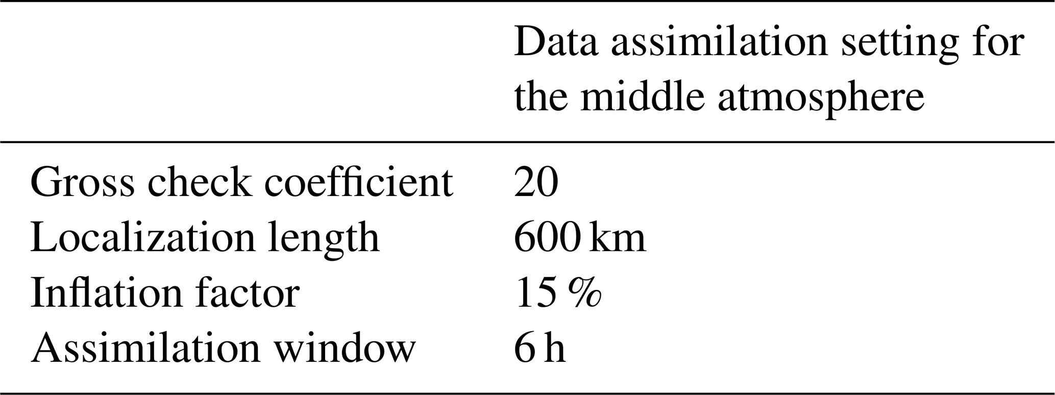
KSMW20 performed a series of sensitivity tests to optimize the data assimilation parameters for the system with 30 ensemble members, such as the degree of gross error check, localization length, inflation factor, and assimilation window. The results are summarized in Table 1. In the present study, the assimilation system with the optimized parameters from KSMW20 is improved by introducing IAU, changing the order of diffusion, and assimilating SABER and SSMIS observations.
Table 1Parameters obtained in Koshin et al. (2020) for the assimilation system of the whole neutral atmosphere.
2.2 Incremental analysis updating (IAU)
The IAU is one of the data insertion schemes used during analysis updates (Bloom et al., 1996). For the IAU, the increments are divided into a small fraction and added at each time step for a finite time period. According to Bloom et al. (1996), the IAU properties are better than those of nudging schemes because the IAU has a sharper response function with less phase distortion.
In our data assimilation cycle, the analysis increments are calculated at t=00:00, 06:00, 12:00, and 18:00 UTC, using the forecasts and observations for the time period from t−3 h to t+3 h. The increments for temperature, zonal and meridional winds, specific humidity, and surface pressure are added as forcing terms to the model equations at each time step for the time period from t−3 h to t+3 h. Finally, the results of the subsequent 6 h forecast without the IAU forcing are used to calculate the assimilation at the next analysis step. Since this method requires an additional 3 h forecast from t−3 h to t h, the resulting forecast time increases by a factor of . This is smaller than that required by DF. Note that, in our data assimilation system, the assimilation module requires 10 times the amount of computation time as that of the model forecast, which means that there is little time increase for the whole analysis cycle from introducing the IAU. The performance of the IAU is examined by comparing the results with and without IAU. The latter is the same as the “Ctrl” setting in KSMW20. KSMW20 focused on relatively slowly varying components, i.e., components with time scales longer than days. In this study, in order to express tides with realistic amplitudes in the assimilation system, the horizontal diffusion of the forecast model is tuned in addition to the IAU inclusion.
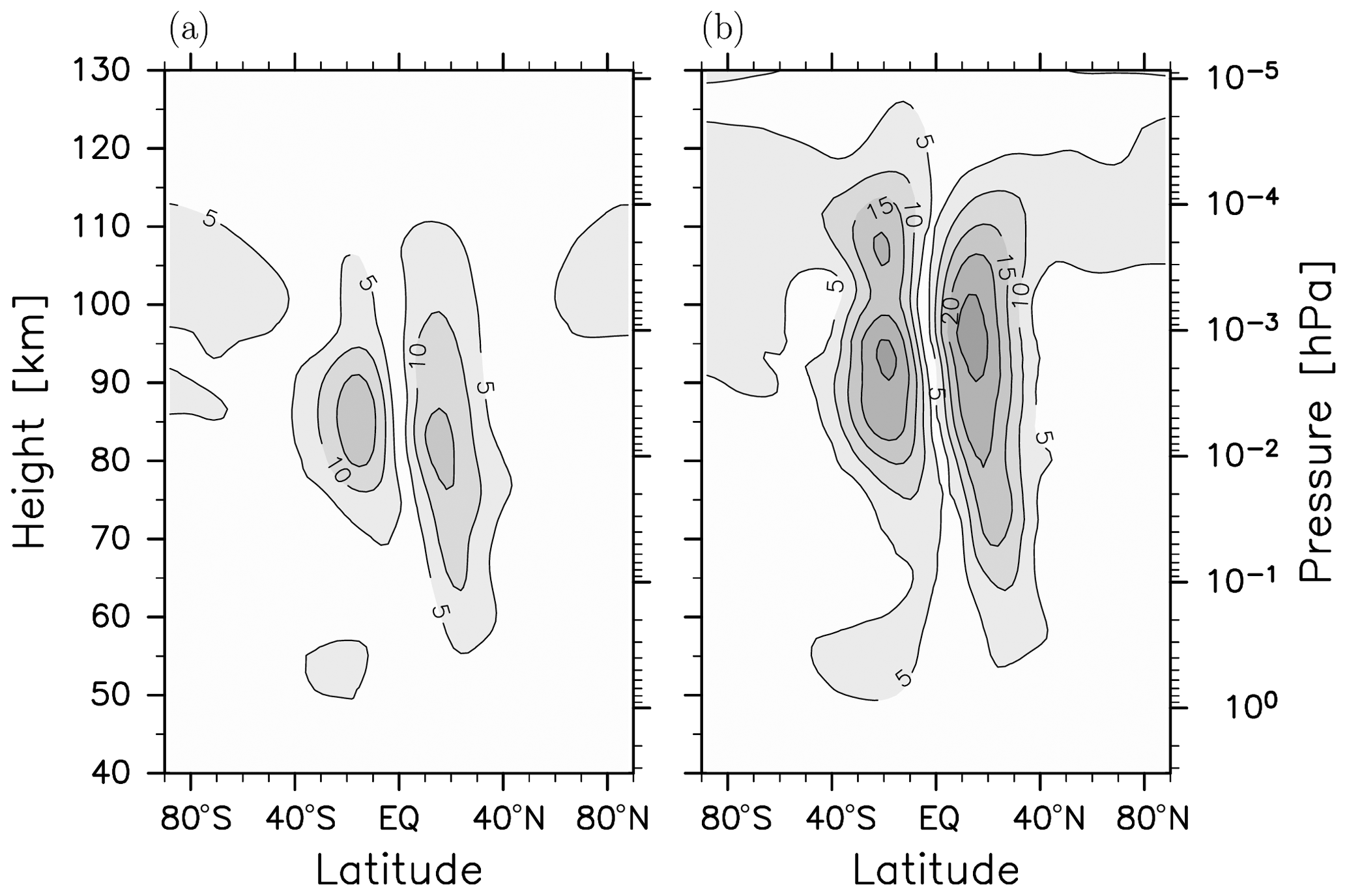
Figure 1Amplitudes of the migrating diurnal tide in the meridional wind from the free-run simulation with (a) the fourth-order horizontal diffusion and (b) the eighth-order horizontal diffusion for the time period from 15 January to 20 February 2017. The contour interval is 5 m s−1.
2.3 The order of diffusion
Figure 1a shows the meridional wind amplitude of the migrating diurnal tide (DW1) in the latitude-height section from the free-run simulation using the forecast model. The tidal amplitude has two broad maxima at altitudes between 70 and 90 km at latitudes of ∼20∘ N and ∼20∘ S. The peak amplitudes are about 20 m s−1, which is roughly a half of the observation from the Wind Imaging Interferometer (WINDII) (e.g., McLandress et al., 1996) and also a half of that realistically simulated by GCMs (e.g., Watanabe and Miyahara, 2009).
The KSMW20 system uses the numerical model with a fourth-order (i.e., ∇4) horizontal hyperdiffusion. The order of the diffusion determines the degree of the relaxation depending on the horizontal wavenumber. Higher-order form can weaken the diffusion for large-scale waves and strengthen that for small-scale waves. Thus, to obtain more realistic tidal amplitudes, the horizontal hyperdiffusion of the eighth-order (i.e., ∇8) is employed. The e-folding time of the horizontal diffusion as a function of the wavenumber for each setting is shown in the Supplement. Figure 1b shows the tidal amplitude from a free-run simulation using the eighth-order diffusion. The peak amplitude is 28 m s−1, which is comparable to that shown by McLandress et al. (1996) and Watanabe and Miyahara (2009).
2.4 SABER
The SABER instrument onboard the TIMED satellite was launched in 2001. This satellite is not in a sun-synchronous orbit, and hence the local time of the measurements is not constant, which is one of the major differences from the MLS. About every 60 d, the satellite performs yaw maneuvers so that data for the regions 53∘ S–83∘ N and 83∘ S–53∘ N are alternately obtained every 60 d. Temperature data retrieved from CO2 infrared limb radiance (Remsberg et al., 2008) are used for the assimilation in our system. We used version 2.0 data. The data are distributed in the altitude range from about 15 to 110 km at ∼1 km intervals. The measurement uncertainty (available from http://saber.gats-inc.com/temp_errors.php, last access: 14 March 2022) is linearly interpolated in the vertical direction and used as observational errors in the assimilation. For example, the uncertainty values are 1.3 K at the altitude of 20 km, 2.0 K at 60 km, and 10.5 K at 100 km. Similarly to the assimilation of the MLS temperature data in KSMW20, the observations are horizontally averaged for the along-track direction to reduce the resolution so that it will be comparable to the forecast model resolution before the assimilation.
2.5 SSMIS
The SSMIS instrument measures Earth's radiation in 24 microwave channels using a conical scan cycle with a swath width of ∼1700 km (Swadley et al., 2008). One SSMIS sensor on the DMSP F17 satellite is currently in operation, although four SSMIS instruments on DMSP satellites (F16, F17, F18, and F19) were launched. The brightness temperatures from six upper air sounding channels in a unified pre-processing package dataset are used for the assimilation. These channels measure the 60 GHz molecular oxygen absorption band, which is sensitive to temperatures in the upper stratosphere and mesosphere. The noise equivalent delta temperature for each channel (available from: https://directory.eoportal.org/web/eoportal/satellite-missions/d/dmsp-block-5d, last access: 14 March 2022) is used as the observational error in our data assimilation system. The horizontal distribution of the SSMIS observation data is denser than the model resolution. To reduce the computational cost, the observations are thinned by taking one of every 10th consecutive data points for both the along- and cross-track directions.
To assimilate the brightness temperature, we implement an observation operator for the SSMIS brightness temperature. The observation operator that converts the model variables to brightness temperatures with a radiative transfer model (RTTOV v.11.3; Saunders et al., 2018) is used, which was originally developed by Terasaki and Miyoshi (2017). The satellite radiances may include two kinds of biases: air-mass-dependent and scan-dependent biases (e.g., Miyoshi et al., 2010). The air-mass bias is responsible for inaccuracies in the radiative transfer calculations, which are correlated with predictors computed from the model variables. In the present study, the air-mass bias is subtracted from the observed radiances following Terasaki and Miyoshi (2017). This correction relies on a linear combination of a set of state-dependent predictors including lapse rate and surface temperature. The coefficients of the predictors are estimated with the ensemble-based variational bias correction method (VarBC; Miyoshi et al., 2010). The scan bias comes from viewing the angles of the field of view. Since the viewing angle is constant for the SSMIS because of the conical scan pattern, there is no need to take the scan bias into consideration for the present assimilation system.
2.6 Independent data
The zonal winds obtained from the assimilation experiments are compared with observations by meteor radars at Longyearbyen (78.2∘ N, 16.0∘ E; Hall et al., 2002), Kototabang (0.2∘ S, 100.3∘ E; Batubara et al., 2011), and Davis Station (68.6∘ S, 78.9∘ E; Murphy, 2017). These radar observations are not assimilated and, thus, can be used for validation as independent reference data. In the following comparison, the data averaged for the height range of 80–88 km were used. We obtained qualitatively similar results also for the meridional winds, although they are not shown.
Table 2Notation for the different experiments considered in this study.
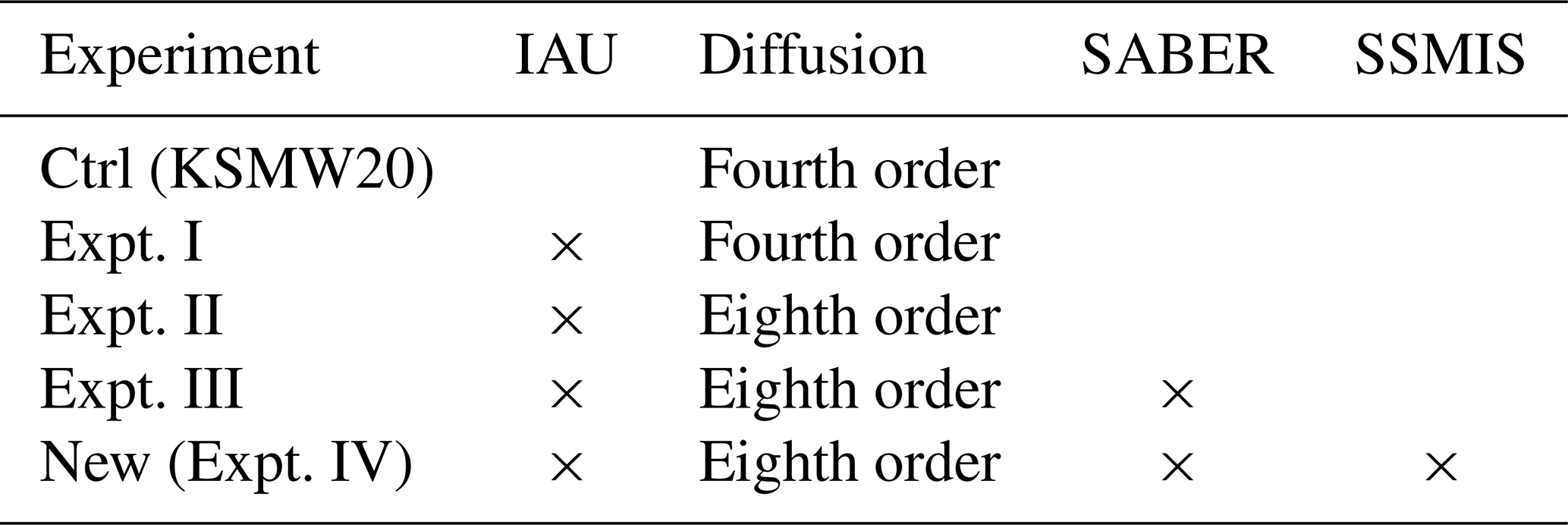
To examine the impacts of these changes in the assimilation system, we performed several assimilation experiments for the whole neutral atmosphere up to the lower thermosphere for the time period of 10 January through 28 February 2017. This period is the same as that focused on by KSMW20. We followed the experiment settings in KSMW20 including the spin-up time and the assimilation parameters. Table 2 summarizes the experiments that we performed. The assimilation system developed by KSMW20 and the analysis data calculated from the system are called the KSMW20 system and Ctrl analysis, respectively. The experiment with the system adopting the IAU filtering is called Expt. I. The comparison between Ctrl and Expt. I analyses shows the impact of the filtering on the reduction of spurious waves generated from analysis increments. The experiment using the forecast model with a tuned horizontal diffusion in addition to the IAU to improve the reproduction of the tidal amplitudes in the analysis is called Expt. II. In Expt. III, the SABER observations are additionally assimilated for the same setting as Expt. II. The system in Expt. IV assimilates the SSMIS observations in addition to the Expt. III setting. Expt. IV is regarded as the new assimilation system developed in the present study.
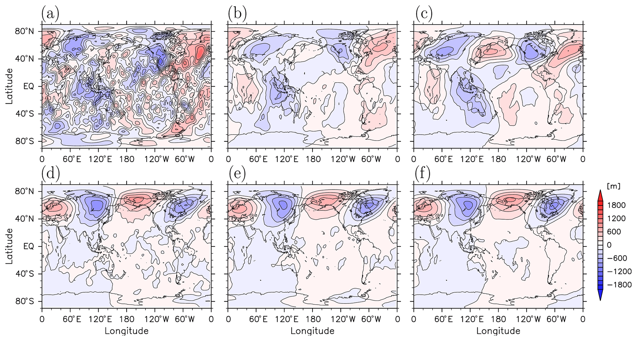
Figure 2(a–c) The longitude–latitude sections of the geopotential height anomaly from the zonal mean in 00:00 UTC on 20 January 2017 at 0.1 hPa from (a) the Ctrl (KSMW20) analysis, (b) the analysis with the IAU (Expt. I), and (c) the MERRA-2 reanalysis. The contour intervals are 200 m. (d–f) Same as (a–c) but for 10 hPa.
3.1 Introducing IAU to the KSMW20 system
The adjustment of the increment can generate spurious waves. They can be suppressed by introducing the IAU. To visualize the effect of introducing the IAU, we made Fig. 2, which shows longitude–latitude sections of the geopotential height anomaly from the zonal mean at 0.1 and 10 hPa at 00:00 UTC on 20 January 2017. First, the analysis produced by the KSMW20 system with the IAU (Expt. I; Fig. 2a and d) is compared with Ctrl analysis (Fig. 2b and e). The MERRA-2 reanalysis, which also adopts the IAU filtering, is shown for comparison (Fig. 2c and f). Disturbances with small scales of about 1000 km are conspicuous in the original analysis at 0.1 hPa (Fig. 2a), while these disturbances are not obvious in the analysis with the IAU (Fig. 2b) or the MERRA-2 reanalysis (Fig. 2c). At 10 hPa, analyses both with (Fig. 2e) and without (Fig. 2d) the IAU filtering show a wave-2 pattern in the extratropics of the Northern Hemisphere causing a split of the polar vortex, although weak smaller-scale disturbances are present only in Ctrl analysis (Fig. 2d). It should be noted that a free-running model simulation with the same initial condition, which by definition has no analysis increments, does not show such small-scale structures (not shown). Thus, most of the small-scale disturbances in the original analysis are likely due to spurious waves generated from the analysis increments. The small-scale waves are reduced through the IAU and the resultant analysis product is similar to the MERRA-2 reanalysis (Fig. 2f).

Figure 3The vertical profiles of standard deviation for small-scale (wavenumber s>21) components of geopotential height at 70∘ N in 00:00 UTC on 20 January 2017 at 0.1 hPa. Black and red curves denote results from the Ctrl (KSMW20) and Expt. I, respectively.
The amplitudes of small-scale waves are relatively large at the higher altitudes. Figure 3 shows the vertical profiles of the standard deviation of geopotential height for waves with zonal wavenumbers larger than 21 at 70∘ N at 00:00 UTC on 20 January 2017. The standard deviation of geopotential height for the Ctrl analysis (black curve) increases above the height of 50 km and is larger than 13 m above the height of 70 km. On the other hand, the standard deviation of geopotential height for the analysis using the IAU (Expt. I; red curve) is smaller than 3 m above the height of 60 km. This is partly due to potentially large increments because of a model bias in the MLT region (Pedatella et al., 2014) and partly due to the amplification of the spurious waves propagating from below due to the exponentially decreasing air density. The IAU suppresses the generation of the spurious waves by reducing the increment at a time step at all heights, and hence effectively suppresses both spurious waves caused in situ and those originating from lower altitudes. It is worth noting here that we conducted sensitivity experiments in which assimilation parameters including the ensemble size and the inflation factor of observation errors were tuned. However, these parameter tunings have little impact on the reduction of the spurious waves compared with the IAU.
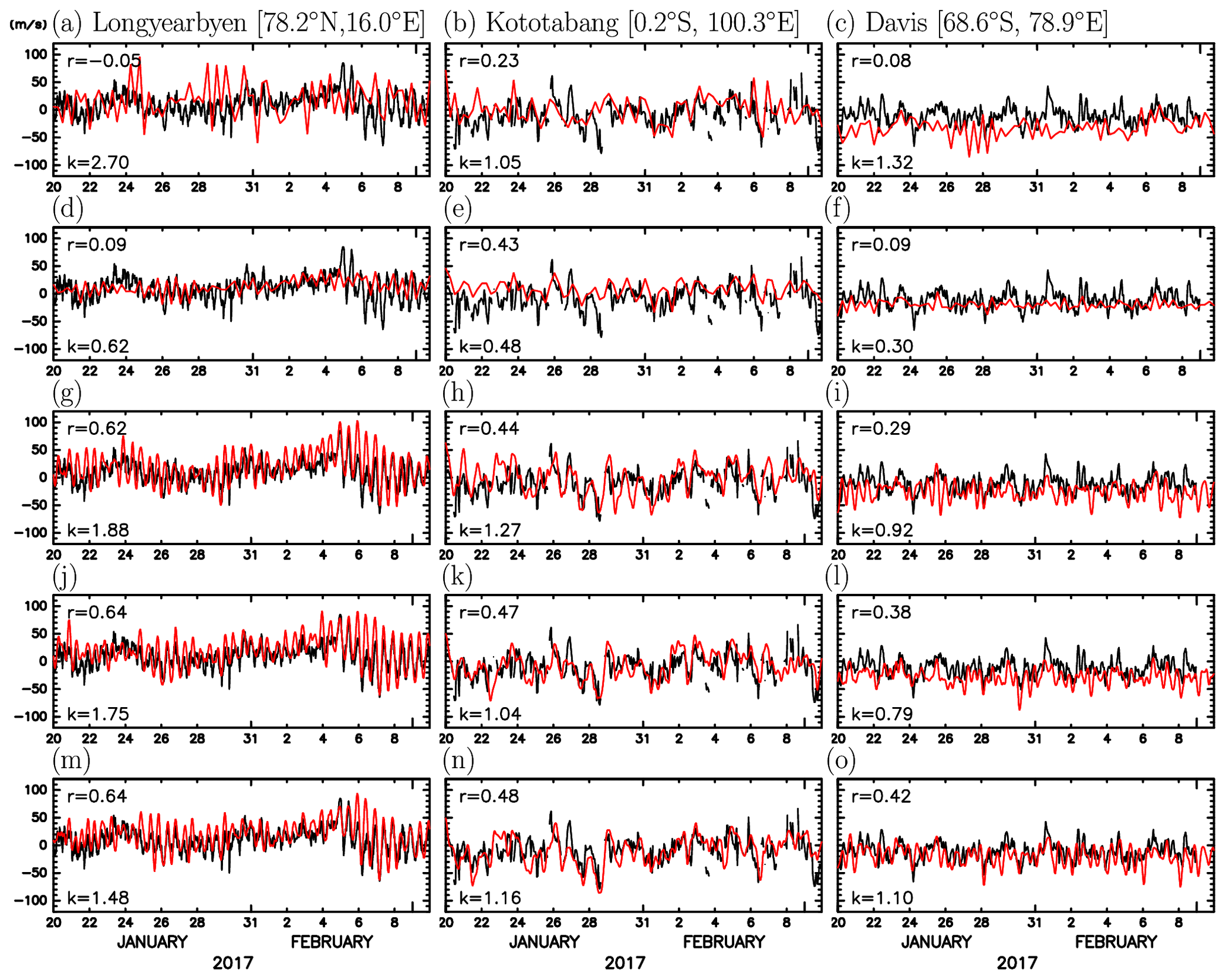
Figure 4The time series of the zonal wind from analysis (red curves) and observations (black curves) by meteor radars at Longyearbyen in the Arctic (a, d, g, j, m), Kototabang near the Equator (b, e, h, k, n), and Davis Station in the Antarctic (c, f, i, l, o). The results for (top to bottom) the Ctrl (KSMW20) analysis, Expt. I, Expt. II, Expt. III, and Expt. IV (New). Each panel lists the correlation coefficient r and ratio of the variances k between the analysis and corresponding meteor radar wind time series.
3.2 Tuning of the horizontal diffusion in the GCM
KSMW20 shows good agreement between their analysis and independent observations from meteor radars for fluctuations with periods longer than several days. However, there are some discrepancies in amplitudes and phases for fluctuations with periods shorter than 1 d. Figure 4a–c show the time series of zonal winds observed by meteor radars at three stations of Longyearbyen, Kototabang, and Davis Station (black curves) and corresponding data from the Ctrl analysis (red curves). At Longyearbyen and Kototabang, the dominant wave periods are about 12 and 24 h, respectively (left and middle panels). At Davis, two kinds of fluctuations with periods of about 12 h and about 2 d seem dominant (right panel). The Ctrl analysis captures the relatively long-period variations at Kototabang, but significant differences are observed for fluctuations with periods shorter than 1 d. This is the case also for the other two stations. The correlation coefficients between the radar and Ctrl analysis time series are small at all stations.
Figure 4d–f show the zonal wind fluctuations obtained by Expt. I to see the effect of IAU. The correlation coefficients between the time series of the analysis and observations increase from 0.23 to 0.43 at Kototabang, while they are low at Longyearbyen and Davis. It is notable that the amplitudes of the short-period variation in Expt. I became significantly underestimated at all stations. The ratio (k) of the wind variance for the analysis to that for the observation is calculated at each station. It is found that the variance in the analysis is in a range of about 40 %–70 % of that in the observation at all stations. We confirmed that the variance for the meridional wind fluctuations in the analysis is also small compared with radar observations at each station. Thus, the realistic amplitudes of short-period fluctuations obtained by the Ctrl analysis (Fig. 4a–c) could be accidental. Therefore, the amplitude of the tides, which are the main components of the short-period fluctuations in the MLT region, in the forecast model is examined.
Figure 4g–i show the results of the assimilation with the same Expt. I, but using the forecast model with the tuned eighth-order diffusion (Expt. II). The results from Expt. II show similar time variations to the radar observations, particularly for the short-period fluctuations. Owing to the improved reproducibility of the semidiurnal variation, the correlation coefficient between the analysis and the radar observation significantly increases from less than 0.1 to 0.6 at Longyearbyen and 0.3 at Davis. Note that the ratio of the variances k at Davis is almost one, whereas those at Longyearbyen and Kototabang are slightly larger than one. The value k=1 means the variance of the analysis and that of observation are the same.
It is also interesting that the introduction of the IAU changes the time mean zonal wind at Davis. The Ctrl analysis shows a negative bias in the zonal wind compared with the observation at Davis (Fig. 4c). The bias for the analyses from Expt. I and Expt. III, which are experiments of the IAU (Fig. 4f and i), is significantly reduced. As will be shown later, this is likely related to the reproducibility of wave forcing in the MLT region.
3.3 Assimilating SABER and SSMIS observations
Finally, we add the data to the assimilation using Expt. II that are from non-sun-synchronous satellites at local times which are different from those of MLS. Figure 4j–l show the time series from the analysis, in which the SABER observation is assimilated (Expt. III). Figure 4m–o show the time series from the analysis, in which the SABER and SSMIS observations are assimilated (Expt. IV; New). It is emphasized that both Expt. III and Expt. IV experiments include the IAU and use the forecast model with the tuned eighth-order diffusion as shown in Table 2. The assimilation of these additional observations increases the correlation coefficients at all stations, particularly for Davis. This result indicates that the constraint from assimilating the observations at different local times is crucial for reproducing tides with realistic amplitude variation. At Longyearbyen and Kototabang, the variances of the time series become closer to those of the observations by assimilating the SABER and SSMIS data. Values of k are obtained within a range from 1.1 to 1.5 for Expt. IV (New). At Longyearbyen in the Arctic, the performance of the assimilation is best in Expt. IV in terms of k while the correlation coefficients are comparable for Expts. II, III, and IV. At Kototabang in the equatorial region, Expt. IV (New) shows the best correlation with the radar observations, although the difference in k among Expts. II, III, and IV is not significant. At Davis, the improvement of the correlation by the assimilation of the SSMIS observation is larger than at the other two stations. This is because there are no SABER observations in the Southern Hemisphere polar region during the present analysis period. Thus, the assimilation of SSMIS observation has more impact at Davis in the Antarctic.
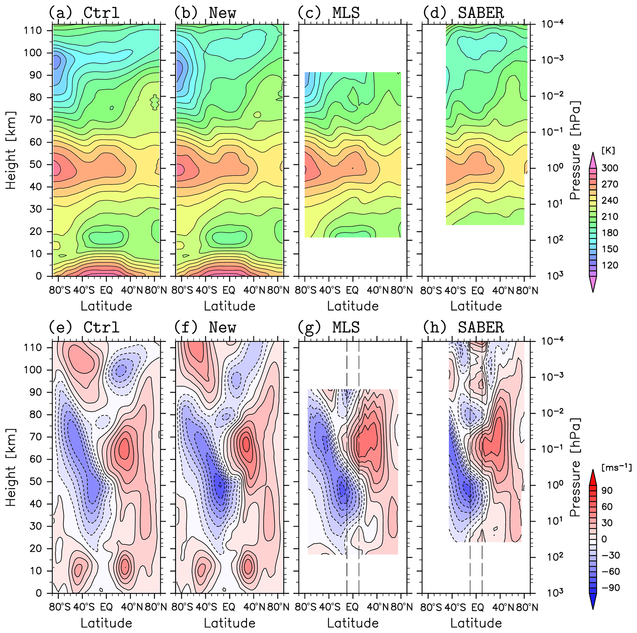
Figure 5(a–d) Zonal mean temperature and (e–h) zonal wind for the time period of 15 January to 20 February 2017. The results in panels (a) and (e) are from the Ctrl (KSMW20) analysis, (b) and (f) are from the new analysis (Expt. IV), (c) and (g) are from the MLS observations, and (d) and (h) are from the SABER observations. The gradient winds from the satellite observations (g, h) at 10∘ S–10∘ N are linearly interpolated. Contour intervals are 10 K for (a–d) and 10 m s−1 for (e–h).
3.4 Comparison with the Ctrl (KSMW20) analysis
In this section, results from Expt. IV (New) are compared in detail with those from Ctrl analysis to examine the performance of the new assimilation system. Figure 5a, b, e, and f show the zonal mean temperature and zonal wind from respective analyses averaged for the time period of 15 January to 20 February 2017. It is seen that the temperature and zonal wind below ∼10 hPa exhibit only slight differences. In the new analysis, the easterly jet in the summer upper stratosphere is strong and its core shifts equatorward compared with the Ctrl analysis. Also, there are significant differences in the zonal wind in the MLT region, such as the height of the zero-wind layer. As a reference, the zonal mean temperature and zonal wind estimated using the geopotential height under the assumption of the gradient wind balance with the temperature from the MLS and SABER observations are also shown (Fig. 5c, d, g, and h). The gradient wind cannot be estimated at the Equator where the Coriolis parameter is zero, so the zonal wind at the Equator is obtained from those at 10∘ S and 10∘ N by a linear interpolation. The jet in the summer upper stratosphere and mesosphere in the new analysis seems close to the gradient wind from the SABER. Here it is worth noting that the gradient winds do not necessarily provide a good approximation of the zonal wind in the low latitudes above a height of ∼80 km where the tidal wave contamination is significant to the data from satellites taking sun-synchronous orbits (Lieberman, 1999) and where the tidal wave forcing in the meridional direction is not negligible (Miyahara et al., 2000).
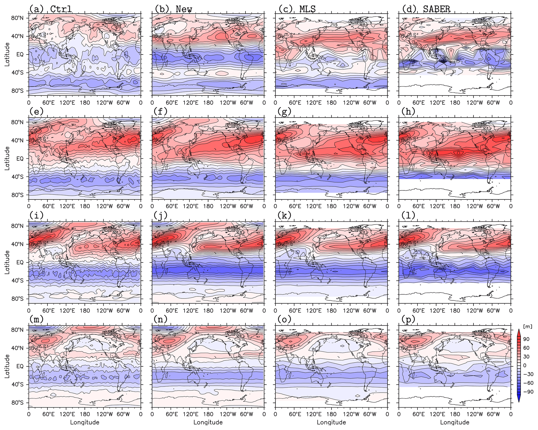
Figure 6The longitude–latitude sections of zonal wind from the analyses and zonal gradient wind from the satellite observations, which are averaged for the time period of 10–20 February 2017 at 0.01 hPa (a–d), 0.1 hPa (e–h), 1 hPa (i–l), and 10 hPa (m–p). The results in panels (a), (e), (i), and (m) are from the Ctrl (KSMW20) analysis, (b), (f), (j), and (n) are from the new analysis (Expt. IV), (c), (g), (k), and (o) are from the MLS observations, and (d), (h), (l), and (p) are from the SABER observations. The gradient winds from the satellite observations (two right columns) at 10∘ S–10∘ N are linearly interpolated. Contour intervals are 10 m s−1.
Figure 6 shows longitude–latitude sections of the zonal wind and zonal gradient wind at 0.01, 0.1, 1, and 10 hPa (from the top to the bottom) averaged for 10–20 February 2017. The difference in the large-scale structure between the Ctrl and the new (i.e., Expt. IV) analyses is evident at 0.01 hPa. The polar night jet structure in the northern midlatitudes at 0.01 hPa in the new analysis is more similar to those of the gradient winds from MLS and SABER. The easterly winds at low latitudes for the new analysis, which are stronger than those in the Ctrl analysis, are close to the gradient wind from SABER. The zonal winds from the Ctrl analysis at 0.1, 1, and 10 hPa have large-amplitude small-scale structures, which are likely due to the spurious waves generated by the analysis increments. In contrast, the new (Expt. IV) analysis shows a smoother horizontal distribution of the zonal wind at all levels. These results reflect the application of the IAU filtering and the assimilation of additional data from the SABER and SSMIS observations. Note that the non-zonal structure of SABER winds at low latitudes are mainly because of the non-uniform location and local time of the orbits (not shown).
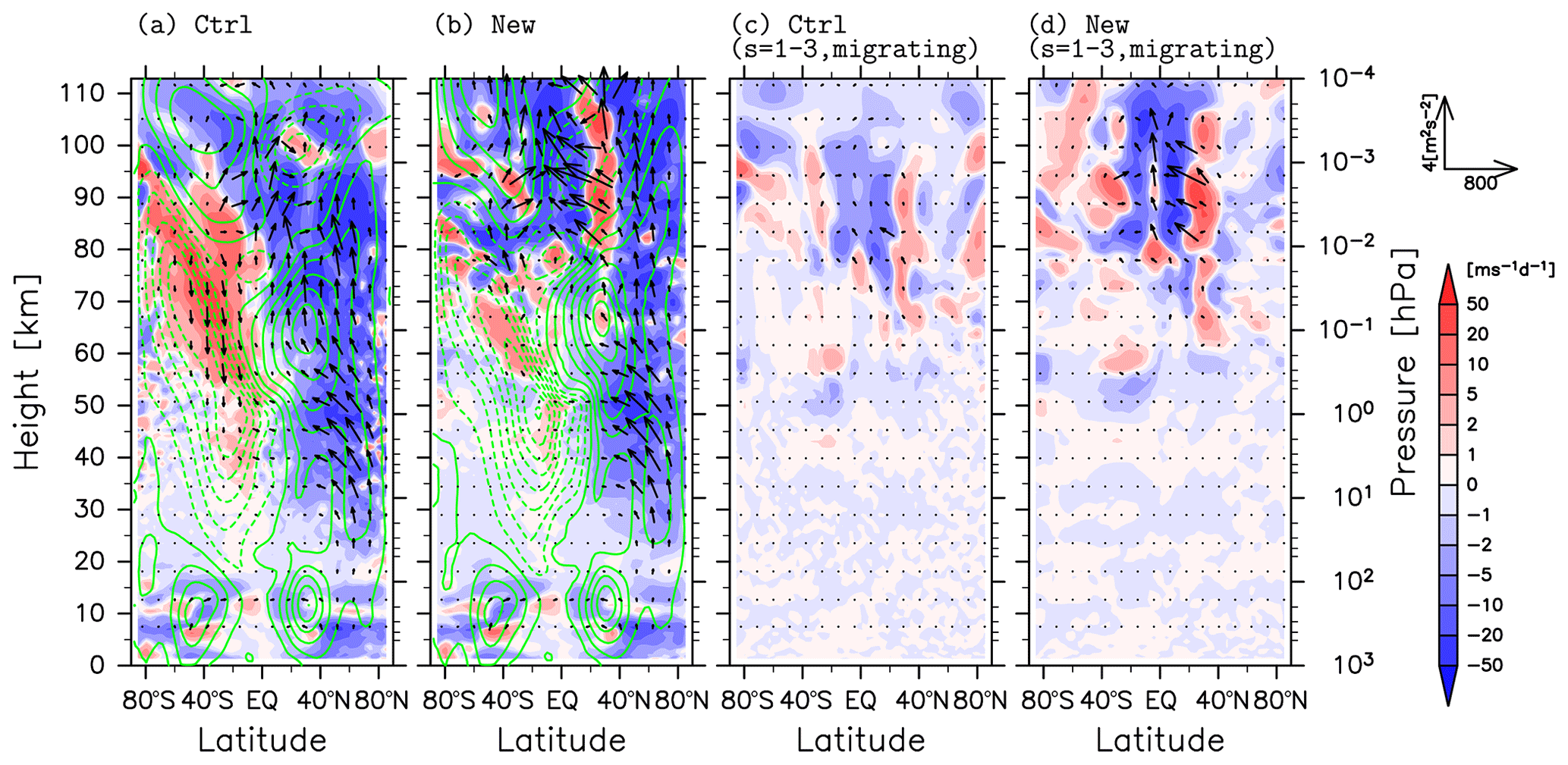
Figure 7(a, b) The zonal mean zonal wind (green contours), E-P flux (arrows), and E-P flux divergence (colors) averaged for the period of 15 January to 20 February 2017. The E-P flux of panel (a) is the result of all the waves for the Ctrl (KSMW20) analysis and that of (b) for the new (Expt. IV) analysis. Contour intervals are 10 m s−1. (c, d) Same as (a, b) but for the E-P flux and E-P flux divergence for the migrating large-scale (wavenumber s<4) waves.
Figure 7 shows the meridional cross sections of the zonal mean zonal wind, Eliassen-Palm (E-P) flux, and its divergence averaged for the time period of 15 January to 20 February 2017. Similar to the zonal wind and temperature, only slight differences in the E-P flux and its divergence (i.e., wave forcing) between the Ctrl and new analyses are seen below ∼10 hPa. The E-P flux divergence from the Ctrl analysis shows a patchy structure in high latitude regions from 10 to 0.1 hPa (Fig. 7a). This is primarily caused by the small-scale spurious waves generated by the assimilation increments (Fig. 2a). The patchy structure mostly disappears in the new analysis (Fig. 7b).
The absolute value of the wave forcing of the new analysis in the MLT region is more than twice that of the Ctrl analysis. To examine the cause of the difference in the wave forcing in the MLT region, the E-P flux for migrating tides are analyzed. Figure 7c and d show the E-P flux for the migrating solar tides with zonal wavenumbers of s=1–4. A relatively large difference in wave forcing because of the migrating tides is observed, particularly, in the equatorial MLT region. Thus, the main reason for the difference in the wave forcing in the MLT region is that the amplitude of tides becomes realistic in the new analysis (Fig. 1).
Below the weak wind layer at heights of 75–90 km in 30–80∘ S in the mesosphere, the sign of the E-P flux divergence and the direction of the vertical component of the E-P flux are opposite between the Ctrl and Expt. IV (New) for each analyses (Fig. 7a and b). It is found that the difference is large for small-scale waves with zonal wavenumbers larger than seven (not shown). In the Ctrl analysis, these small-scale waves are mainly attributable to the upward propagating spurious waves (not shown). Thus, the suppression of the spurious waves by adapting the IAU filtering is likely responsible for the difference in the wave forcing in the southern mesosphere. Besides, it is considered that the increase in the number of satellite observations and the change in the horizontal diffusion from the new assimilation system also improve the representation of small-scale waves in the MLT region. It is interesting to note that, around the weak wind layer at 40∘ S, the difference in the zonal mean zonal wind between the Ctrl analysis and the new analysis is smaller than 10 m s−1 in spite of the significant difference in the wave forcing.
The data assimilation system for the height region from the surface to the lower thermosphere developed by KSMW20 was updated to better represent disturbances with wave periods shorter than 1 d such as atmospheric tides, which have large amplitudes and may induce significant wave forcing in the MLT region. In the present study, (i) the IAU filtering was introduced, (ii) the order of horizontal diffusion (hyperdiffusion) was changed, and (iii) observations from the SABER and SSMIS were also assimilated (Expt. IV; see Table 2). The validity of the analysis was confirmed by comparison with independent data, i.e., horizontal winds from meteor radar observations at Longyearbyen in the Arctic, at Kototabang in the equatorial region, and at Davis Station in the Antarctic. Details of the results are summarized as follows:
-
Large amplitudes of disturbances with small horizontal scales of about 1000 km in the MLT region observed in the Ctrl analysis by KSMW20 were attributable to the analysis increments, because these disturbances were not observed in the free-run simulation with the same initial condition. Thus, first, the IAU filtering was introduced. This improvement could efficiently reduce these spurious waves and produce more realistic fields for small-scale waves.
-
Next, to obtain realistic tidal wave amplitudes in the MLT region, a horizontal hyperdiffusion of the eighth order was introduced so that only small-scale fluctuations could be effectively diffused. The tidal wave amplitudes in the time series of the zonal wind from the new analysis became reasonable but still were somewhat larger than those from the meteor radar observations.
-
Last but not least, the SABER temperature retrieval and SSMIS brightness temperature retrieval in the stratosphere and mesosphere were also assimilated. The correlation between the horizontal wind time series estimated by this new assimilation method and those from meteor radar observations became higher. The amplitudes of the horizontal wind fluctuations in the upper mesosphere also became closer to those from the radar observations.
It was shown that assimilation of both sun-synchronous and non-sun-synchronous satellite observations is important for better representation of the zonal mean field as well as for short-period fluctuations such as tides. In fact, at Longyearbyen, the quasi-half-day fluctuations with large amplitudes observed by the meteor radar are well reproduced in the present analysis (Fig. 4m). The correlation between the radar observations and the products of our assimilation system using both types of satellite observations is high (around 0.64), but not very high. This may be partly because of the existence of unresolved gravity waves in our model. Shibuya et al. (2017) simulated the 12 h period disturbances that are observed by a mesosphere–stratosphere–troposphere radar (a VHF clear-air Doppler radar) at Syowa Station in the Antarctic in winter using a high-resolution high-top GCM and showed that they are due to inertia–gravity waves with horizontal wavelengths of 1000–2000 km. Such relatively short horizontal waves are hardly simulated by the numerical model with T42 used in our assimilation system.
It is worth noting that the mean winds are well reproduced even by our previous assimilation system (KSMW20 system), although a slight bias remained. However, the wave-forcing properties have been largely modified. For example, around the weak wind layer in the mesosphere of the Southern Hemisphere, the sign of E-P flux divergence and the direction of the vertical component of the E-P flux are opposite between the previous (KSMW20) and the new analyses. These are mainly attributable to the reduction of spurious small-scale waves caused by assimilation increments. In the equatorial MLT region, the deceleration of the westerly wind associated with the E-P flux convergence in the new analysis is also modified. This is because of better representation of tidal waves there. Such better reproduction of waves improved by the new assimilation will allow us to study the momentum budget in the MLT region, including tidal waves, quantitatively.
Our data assimilation system employs the 4D-LETKF method. Therefore, the computational cost is low. We plan to carry out a long-period analysis using the new assimilation system updated in the present study, over about 16 years from the start of the MLS observations in August 2004 to the present, to examine the dynamics of the MLT variations at time scales from days to years.
For legal reasons, the source code for the forecast model, data assimilation module, and run scripts cannot be publicly released. They have been made available to the editor and reviewers, and are available to anyone by contacting the corresponding author. The copyright of the original code for LETKF belongs to Takemasa Miyoshi, and it can be accessed from https://github.com/takemasa-miyoshi/letkf (last access: 26 June 2020, Miyoshi, 2016). Meteor radar data from Kototabang are available at the Inter-university Upper atmosphere Global Observation NETwork (IUGONET) site (http://database.rish.kyoto-u.ac.jp/arch/iugonet/mwr_ktb/index_mwr_ktb.html, last access: 25 January 2021, Abe et al., 2014). Meteor radar data from Longyearbyen are available on request from the National Institute of Polar Research by contacting Masaki Tsutsumi (tutumi@nipr.ac.jp). Meteor radar data from Davis (Murphy, 2017) are available online. NCEP PREPBUFR data are also available online (https://doi.org/10.5065/Z83F-N512, NCEP ADP, 2008). Aura MLS data (https://doi.org/10.5067/Aura/MLS/DATA2021, Schwartz et al., 2015), which are compiled and archived by NASA, were also used for the data assimilation. SABER data can be downloaded from the FTP site at ftp://saber.gats-inc.com/Version2_0/Level2A/ (last access: 19 October 2020). SSMIS data can be downloaded from https://www.avl.class.noaa.gov/saa/products/catSearch (last access: 25 January 2021, SSMIS, 2021). MERRA-2 data (M2I3NPASM) can be downloaded from https://doi.org/10.5067/QBZ6MG944HW0 (GMAO, 2015).
The supplement related to this article is available online at: https://doi.org/10.5194/gmd-15-2293-2022-supplement.
DK, MK, and KS designed the experiments, and DK carried them out. SW developed the forecast model code. DK, MK, and KS prepared the paper with contributions from all the coauthors.
The contact author has declared that neither they nor their coauthors have any competing interests.
Publisher's note: Copernicus Publications remains neutral with regard to jurisdictional claims in published maps and institutional affiliations.
We greatly appreciate Masaki Tsutsumi and Chris Hall for providing the meteor radar data from Longyearbyen. Operation of the Davis meteor radar was supported through Australian Antarctic Science project number 4025 and we deeply thank the project CI Damian Murphy for providing the data. Dai Koshin thanks Kazuyuki Miyazaki for his continuous encouragement. The data assimilation experiments were performed using the Japan Agency for Marine-Earth Science and Technology (JAMSTEC) Data Analyzer (DA) system. The figures were produced by the GFD-DENNOU Library.
This research has been supported by the Japan Science and Technology Agency (Core Research for Evolutional Science and Technology; grant no. JPMJCR1663) and the Japan Society for the Promotion of Science (grant no. 18H01276).
This paper was edited by David Ham and reviewed by two anonymous referees.
Abe, S., Umemura, N., Koyama, Y., Tanaka, Y., Yagi, M., Yatagai, A., Shinbori, A., Ueno, S., Sato, Y., and Kaneda, N.: Progress of the IUGONET system – metadata database for upper atmosphere ground-based observation data, Earth Planets Space, 66, 133, https://doi.org/10.1186/1880-5981-66-133, 2014.
Anderson, J. L.: An Ensemble Adjustment Kalman Filter for Data Assimilation, Mon. Weather Rev., 129, 2884–2903, https://doi.org/10.1175/1520-0493(2001)129<2884:AEAKFF>2.0.CO;2, 2001.
Anderson, J. L., Hoar, T., Raeder, K., Liu, H., Collins, N., Torn, R., and Avellano, A.: The Data Assimilation Research Testbed: A Community Facility, B. Am. Meteorol. Soc., 90, 1283–1296, https://doi.org/10.1175/2009BAMS2618.1, 2009.
Batubara, M., Suryana, R., Manik, T., and Sitompul, P.: Kototabang – West Sumatera meteor radar: System design and initial results of a large scale meteor echo, TSSA, 17–21, https://doi.org/10.1109/TSSA.2011.6095399, 2011.
Becker, E.: Dynamical Control of the Middle Atmosphere, Space Sci. Rev., 168, 283–314, https://doi.org/10.1007/s11214-011-9841-5, 2012.
Bloom, S. C., Takacs, L. L., da Silva, A. M., and Ledvina, D.: Data Assimilation Using Incremental Analysis Updates, Mon. Weather Rev., 124, 1256–1271, https://doi.org/10.1175/1520-0493(1996)124<1256:DAUIAU>2.0.CO;2, 1996.
Eckermann, S. D., Ma, J., Hoppel, K. W., Kuhl, D. D., Allen, D. R., Doyle, J. A., Viner, K. C., Ruston, B. C., Baker, N. L., Swadley, S. D., Whitcomb, T. R., Reynolds, C. A., Xu, L., Kaifler, N., Kaifler, B., Reid, I. M., Murphy, D. J., and Love, P. T.: High-Altitude (0–100 km) Global Atmospheric Reanalysis System: Description and Application to the 2014 Austral Winter of the Deep Propagating Gravity Wave Experiment (DEEPWAVE), Mon. Weather Rev., 146, 2639–2666, https://doi.org/10.1175/MWR-D-17-0386.1, 2018.
Ern, M., Preusse, P., Kalisch, S., Kaufmann, M., and Riese, M.: Role of gravity waves in the forcing of quasi two-day waves in the mesosphere: An observational study, J. Geophys. Res.-Atmos., 118, 3467–3485, https://doi.org/10.1029/2012JD018208, 2013.
Fritts, D. C. and Vincent, R. A.: Mesospheric Momentum Flux Studies at Adelaide, Australia: Observations and a Gravity Wave–Tidal Interaction Model, J. Atmos. Sci., 44, 605–619, https://doi.org/10.1175/1520-0469(1987)044<0605:MMFSAA>2.0.CO;2, 1987.
Gelaro, R., McCarty, W., Suárez, M. J., Todling, R., Molod, A., Takacs, L., Randles, C. A., Darmenov, A., Bosilovich, M. G., Reichle, R., Wargan, K., Coy, L., Cullather, R., Draper, C., Akella, S., Buchard, V., Conaty, A., da Silva, A. M., Gu, W., Kim, G., Koster, R., Lucchesi, R., Merkova, D., Nielsen, J. E., Partyka, G., Pawson, S., Putman, W., Rienecker, M., Schubert, S. D., Sienkiewicz, M., and Zhao, B.: The Modern-Era Retrospective Analysis for Research and Applications, Version 2 (MERRA-2), J. Climate, 30, 5419–5454, https://doi.org/10.1175/JCLI-D-16-0758.1, 2017.
Geller, M. A., Alexander, M. J., Love, P. T., Bacmeister, J., Ern, M., Hertzog, A., Manzini, E., Preusse, P., Sato, K., Scaife, A. A., and Zhou, T.: A Comparison between Gravity Wave Momentum Fluxes in Observations and Climate Models, J. Climate, 26, 6383–6405, https://doi.org/10.1175/JCLI-D-12-00545.1, 2013.
GMAO: MERRA-2 inst3_3d_asm_Np: 3d, 3-Hourly, Instantaneous, Pressure-Level, Assimilation, Assimilated Meteorological Fields V5.12.4, Greenbelt, MD, USA, Goddard Earth Sciences Data and Information Services Center (GES DISC) [data set], https://doi.org/10.5067/QBZ6MG944HW0, 2015.
Gumbel, J. and Karlsson, B.: Intra- and inter-hemispheric coupling effects on the polar summer mesosphere, Geophys. Res. Lett., 38, L14804, https://doi.org/10.1029/2011GL047968, 2011.
Hall, C. M., Husly, B. O., Aso, T., and Tsutsumi, M.: The Nippon/Norway Svalbard Meteor Radar: First results of small-scale structure observations, Chinese J. Polar Sci., 13, 47–54, 2002.
Hogan, T., Liu, M., Ridout, J., Peng, M., Whitcomb, T., Ruston, B., Reynolds, C., Eckermann, S., Moskaitis, J., Baker, N., McCormack, J., Viner, K., McLay, J., Flatau, M., Xu, L., Chen, C., and Chang, S.: The Navy Global Environmental Model, Oceanography, 27, 116–125, https://doi.org/10.5670/oceanog.2014.73, 2014.
Hoppel, K. W., Baker, N. L., Coy, L., Eckermann, S. D., McCormack, J. P., Nedoluha, G. E., and Siskind, D. E.: Assimilation of stratospheric and mesospheric temperatures from MLS and SABER into a global NWP model, Atmos. Chem. Phys., 8, 6103–6116, https://doi.org/10.5194/acp-8-6103-2008, 2008.
Kalnay, E.: Atmospheric Modeling, Data Assimilation and Predictability, Cambridge University Press, Cambridge, https://doi.org/10.1017/CBO9780511802270, 2002.
Karlsson, B., Randall, C. E., Benze, S., Mills, M., Harvey, V. L., Bailey, S. M., and Russell III, J. M.: Intra-seasonal variability of polar mesospheric clouds due to inter-hemispheric coupling, Geophys. Res. Lett., 36, L20802, https://doi.org/10.1029/2009GL040348, 2009.
Körnich, H. and Becker, E.: A simple model for the interhemispheric coupling of the middle atmosphere circulation, Adv. Space Res., 45, 661–668, https://doi.org/10.1016/j.asr.2009.11.001, 2010.
Koshin, D., Sato, K., Miyazaki, K., and Watanabe, S.: An ensemble Kalman filter data assimilation system for the whole neutral atmosphere, Geosci. Model Dev., 13, 3145–3177, https://doi.org/10.5194/gmd-13-3145-2020, 2020.
Li, D. and Shine, K. P.: UK Universities Global Atmospheric Modelling Programme (UGAMP) Global Ozone Climatology Project Dataset, NCAS British Atmospheric Data Centre, http://badc.nerc.ac.uk/data/ugamp-o3-climatology/ (last access: 4 September 2019), 1999.
Lieberman, R.: The gradient wind in the mesosphere and lower thermosphere, Earth Planet Sp., 51, 751–761, https://doi.org/10.1186/BF03353234, 1999.
Liu, H.-L., Bardeen, C. G., Foster, B. T., Lauritzen, P., Liu, J., Lu, G., Marsh, D. R., Maute, A., McInerney, J. M., Pedatella, N. M., Qian, L., Richmond, A. D., Roble, R. G., Solomon, S. C., Vitt, F. M. and Wang, W.: Development and Validation of the Whole Atmosphere Community Climate Model With Thermosphere and Ionosphere Extension (WACCM-X 2.0), J. Adv. Model. Earth Syst., 10, 381–402, https://doi.org/10.1002/2017MS001232, 2018.
Livesey, N. J., Read, W. G., Wagner, P. A., Froidevaux, L., Lambert, A., Manney. G. L., Millán Valle, L. F., Pumphrey, H. C., Santee, M. L., Schwartz, M. J., Wang, S., Fuller, R. A., Jarnot, R. F., Knosp, B. W., Martinez, E., and Lay, R. R.: Aura Microwave Limb Sounder (MLS) Version 4.2× Level 2 and 3 data quality and description document, https://mls.jpl.nasa.gov/data/v4-2_data_quality_document.pdf, last access: 24 July 2020.
McCormack, J., Hoppel, K., Kuhl, D., de Wit, R., Stober, G., Espy, P., Baker, N., Brown, P., Fritts, D., Jacobi, C., Janches, D., Mitchell, N., Ruston, B., Swadley, S., Viner, K., Whitcomb, T., and Hibbins, R.: Comparison of mesospheric winds from a high-altitude meteorological analysis system and meteor radar observations during the boreal winters of 2009–2010 and 2012–2013, J. Atmos. Solar-Terr. Phy., 154, 132–166, https://doi.org/10.1016/j.jastp.2016.12.007, 2017.
McLandress, C., Shepherd, G. G., and Solheim, B. H.: Satellite observations of thermospheric tides: Results from the Wind Imaging Interferometer on UARS, J. Geophys. Res., 101, 4093–4114, https://doi.org/10.1029/95JD03359, 1996.
Miyahara, S., Yamamoto, D., and Miyoshi, Y.: On the Geostrophic Balance of Mean Zonal Winds in the Mesosphere and Lower Thermosphere, J. Meteorol. Soc. Japan, 78, 683–688, https://doi.org/10.2151/jmsj1965.78.5_683, 2000.
Miyoshi, T.: Local Ensemble Karman Filter, GitHub [code], https://github.com/takemasa-miyoshi/letkf (last access: 14 March 2022), 2016
Miyoshi, T. and Yamane, S.: Local Ensemble Transform Kalman Filtering with an AGCM at a T159/L48 Resolution, Mon. Weather Rev., 135, 3841–3861, https://doi.org/10.1175/2007MWR1873.1, 2007.
Miyoshi, T., Sato, Y., and Kadowaki, T.: Ensemble Kalman Filter and 4D-Var Intercomparison with the Japanese Operational Global Analysis and Prediction System, Mon. Weather Rev., 138, 2846–2866, https://doi.org/10.1175/2010MWR3209.1, 2010.
Murphy, D. J.: Davis 33 MHz Meteor Detection Radar Winds, Australian Antarctic Data Centre [data set], https://data.aad.gov.au/metadata/records/Davis_33MHz_Meteor_Radar (last access: 19 October 2020), 2017.
NCEP ADP: Global Upper Air and Surface Weather Observations (PREPBUFR format), Boulder, CO, Research Data Archive at the National Center for Atmospheric Research, Computational and Information Systems Laboratory [data set], https://doi.org/10.5065/Z83F-N512, 2008.
Pedatella, N. M., Fuller-Rowell, T., Wang, H., Jin, H., Miyoshi, Y., Fujiwara, H., Shinagawa, H., Liu, H.-L., Sassi, F., Schmidt, H., Matthias, V., and Goncharenko, L.: The neutral dynamics during the 2009 sudden stratosphere warming simulated by different whole atmosphere models, J. Geophys. Res.-Space, 119, 1306–1324, https://doi.org/10.1002/2013JA019421, 2014.
Pedatella, N. M., Liu, H.-L., Marsh, D. R., Raeder, K., Anderson, J. L., Chau, J. L., Goncharenko, L. P., and Siddiqui, T. A.: Analysis and Hindcast Experiments of the 2009 Sudden Stratospheric Warming in WACCMX + DART, J. Geophys. Res.-Space Phys., 123, 3131–3153, https://doi.org/10.1002/2017JA025107, 2018.
Plumb, R. A.: Stratospheric Transport, J. Meteorol. Soc. Japan. Ser. II, 80, 793–809, https://doi.org/10.2151/jmsj.80.793, 2002.
Polavarapu, S., Ren, S., Clayton, A. M., Sankey, D., and Rochon, Y.: On the Relationship between Incremental Analysis Updating and Incremental Digital Filtering, Mon. Weather Rev., 132, 2495–2502, https://doi.org/10.1175/1520-0493(2004)132<2495:OTRBIA>2.0.CO;2, 2004.
Polavarapu, S., Ren, S., Rochon, Y., Sankey, D., Ek, N., Koshyk, J., and Tarasick, D.: Data assimilation with the Canadian middle atmosphere model, Atmosphere-ocean, 43, 77–100, https://doi.org/10.3137/ao.430105, 2005.
Rayner, N. A., Parker, D. E., Horton, E. B., Folland, C. K., Alexander, L. V., Rowell, D. P., Kent, E. C., and Kaplan, A.: Global analyses of sea surface temperature, sea ice, and night marine air temperature since the late nineteenth century, J. Geophys. Res., 108, 4407, https://doi.org/10.1029/2002JD002670, 2003.
Remsberg, E. E., Marshall, B. T., Garcia-Comas, M., Krueger, D., Lingenfelser, G. S., Martin-Torres, J., Mlynczak, M. G., Russell III, J. M., Smith, A. K., Zhao, Y., Brown, C., Gordley, L. L., Lopez-Gonzalez, M., Lopez-Puertas, M., She, C.-Y., Taylor, M. J., and Thompson, R. E.: Assessment of the quality of the Version 1.07 temperature-versus-pressure profiles of the middle atmosphere from TIMED/SABER, J. Geophys. Res., 113, D17101, https://doi.org/10.1029/2008JD010013, 2008.
Rienecker, M. M., Suarez, M. J., Gelaro, R., Todling, R., Bacmeister, J., Liu, E., Bosilovich, M. G., Schubert, S. D., Takacs, L., Kim, G., Bloom, S., Chen, J., Collins, D., Conaty, A., da Silva, A., Gu, W., Joiner, J., Koster, R. D., Lucchesi, R., Molod, A., Owens, T., Pawson, S., Pegion, P., Redder, C. R., Reichle, R., Robertson, F. R., Ruddick, A. G., Sienkiewicz, M., and Woollen, J.: MERRA: NASA's Modern-Era Retrospective Analysis for Research and Applications, J. Climate, 24, 3624–3648, https://doi.org/10.1175/JCLI-D-11-00015.1, 2011.
Sankey, D., Ren, S., Polavarapu, S., Rochon, Y. J., Nezlin, Y., and Beagley, S.: Impact of data assimilation filtering methods on the mesosphere, J. Geophys. Res., 112, D24104, https://doi.org/10.1029/2007JD008885, 2007.
Sato, K. and Nomoto, M.: Gravity Wave–Induced Anomalous Potential Vorticity Gradient Generating Planetary Waves in the Winter Mesosphere, J. Atmos. Sci., 72, 3609–3624, https://doi.org/10.1175/JAS-D-15-0046.1, 2015.
Sato, K., Watanabe, S., Kawatani, Y., Tomikawa, Y., Miyazaki, K., and Takahashi, M.: On the origins of mesospheric gravity waves, Geophys. Res. Lett., 36, L19801, https://doi.org/10.1029/2009GL039908, 2009.
Sato, K., Yasui, R., and Miyoshi, Y.: The Momentum Budget in the Stratosphere, Mesosphere, and Lower Thermosphere. Part I: Contributions of Different Wave Types and In Situ Generation of Rossby Waves, J. Atmos. Sci., 75, 3613–3633, https://doi.org/10.1175/JAS-D-17-0336.1, 2018.
Saunders, R., Hocking, J., Turner, E., Rayer, P., Rundle, D., Brunel, P., Vidot, J., Roquet, P., Matricardi, M., Geer, A., Bormann, N., and Lupu, C.: An update on the RTTOV fast radiative transfer model (currently at version 12), Geosci. Model Dev., 11, 2717–2737, https://doi.org/10.5194/gmd-11-2717-2018, 2018.
Schwartz, M., Livesey, N., and Read, W.: MLS/Aura Level 2 Temperature V004, Greenbelt, MD, USA, Goddard Earth Sciences Data and Information Services Center (GES DISC) [data set], https://doi.org/10.5067/Aura/MLS/DATA2021, 2015.
Shepherd, T. G., Koshyk, J. N., and Ngan, K.: On the nature of large-scale mixing in the stratosphere and mesosphere, J. Geophys. Res., 105, 12433–12446, https://doi.org/10.1029/2000JD900133, 2000.
Shibuya, R., Sato, K., Tsutsumi, M., Sato, T., Tomikawa, Y., Nishimura, K., and Kohma, M.: Quasi-12 h inertia–gravity waves in the lower mesosphere observed by the PANSY radar at Syowa Station (39.6∘ E, 69.0∘ S), Atmos. Chem. Phys., 17, 6455–6476, https://doi.org/10.5194/acp-17-6455-2017, 2017.
Smith, A.: Global Dynamics of the MLT, Surv. Geophys., 33, 1177–1230, https://doi.org/10.1007/s10712-012-9196-9, 2012.
Smith, A. K., Pedatella, N. M., Marsh, D. R., and Matsuo, T.: On the Dynamical Control of the Mesosphere–Lower Thermosphere by the Lower and Middle Atmosphere, J. Atmos. Sci., 74, 933–947, https://doi.org/10.1175/JAS-D-16-0226.1, 2017.
SSMIS: SSMIS Unified Pre-Procesed TDRs BUFR, SSMIS [data set], https://www.avl.class.noaa.gov/saa/products/catSearch, last access: 25 January 2021.
Swadley, S. D., Poe, G. A., Bell, W., Ye Hong, Kunkee, D. B., McDermid, I. S., and Leblanc, T.: Analysis and Characterization of the SSMIS Upper Atmosphere Sounding Channel Measurements, TGRS, 46, 962–983, https://doi.org/10.1109/TGRS.2008.916980, 2008.
Terasaki, K. and Miyoshi, T.: Assimilating AMSU-A Radiances with the NICAM-LETKF, J. Meteorol. Soc. Japan. Ser. II, 95, 433–446, https://doi.org/10.2151/jmsj.2017-028, 2017.
Thurairajah, B., Cullens, C. Y., Siskind, D. E., Hervig, M. E., and Bailey, S. M.: The Role of Vertically and Obliquely Propagating Gravity Waves in Influencing the Polar Summer Mesosphere, J. Geophys. Res.-Atmos., 125, e2020JD032495, https://doi.org/10.1029/2020JD032495, 2020.
Vadas, S. L., Zhao, J., Chu, X., and Becker, E.: The Excitation of Secondary Gravity Waves From Local Body Forces: Theory and Observation, J. Geophys. Res.-Atmos., 123, 9296–9325, https://doi.org/10.1029/2017JD027970, 2018.
Wang, H., Fuller-Rowell, T., Akmaev, R. A., Hu, M., Kleist, D. T., and Iredell, M. D.: First simulations with a whole atmosphere data assimilation and forecast system: The January 2009 major sudden stratospheric warming, J. Geophys. Res., 116, A12321, https://doi.org/10.1029/2011JA017081, 2011.
Watanabe, S. and Miyahara, S.: Quantification of the gravity wave forcing of the migrating diurnal tide in a gravity wave–resolving general circulation model, J. Geophys. Res., 114, D07110, https://doi.org/10.1029/2008JD011218, 2009.
Watanabe, S., Tomikawa, Y., Sato, K., Kawatani, Y., Miyazaki, K., and Takahashi, M.: Simulation of the eastward 4-day wave in the Antarctic winter mesosphere using a gravity wave resolving general circulation model, J. Geophys. Res., 114, D16111, https://doi.org/10.1029/2008JD011636, 2009.
Xu, X., Manson, A. H., Meek, C. E., Jacobi, C., Hall, C. M., and Drummond, J. R.: Mesospheric wind semidiurnal tides within the Canadian Middle Atmosphere Model Data Assimilation System, J. Geophys. Res.-Atmos., 116, D17102, https://doi.org/10.1029/2011JD015966, 2011a.
Xu, X., Manson, A. H., Meek, C. E., Jacobi, C., Hall, C. M., and Drummond, J. R.: Verification of the mesospheric winds within the Canadian Middle Atmosphere Model Data Assimilation System using radar measurements, J. Geophys. Res., 116, D16108, https://doi.org/10.1029/2011JD015589, 2011b.
Yasui, R., Sato, K., and Miyoshi, Y.: The Momentum Budget in the Stratosphere, Mesosphere, and Lower Thermosphere. Part II: The In Situ Generation of Gravity Waves, J. Atmos. Sci., 75, 3635–3651, https://doi.org/10.1175/JAS-D-17-0337.1, 2018.
Yasui, R., Sato, K., and Miyoshi, Y.: Roles of Rossby Waves, Rossby-Gravity Waves, and Gravity Waves Generated in the Middle Atmosphere for Interhemispheric Coupling, J. Atmos. Sci., 78, 3867–3888, https://doi.org/10.1175/JAS-D-21-0045.1, 2021.