TopoCLIM: rapid topography-based downscaling of regional climate model output in complex terrain v1.1

This study describes and evaluates a new downscaling scheme that specifically addresses the need for hillslope-scale atmospheric-forcing time series for modelling the local impact of regional climate change projections on the land surface in complex terrain. The method has a global scope in that it does not rely directly on surface observations and is able to generate the full suite of model forcing variables required for hydrological and land surface modelling in hourly time steps. It achieves this by utilizing the previously published TopoSCALE scheme to generate synthetic observations of the current climate at the hillslope scale while accounting for a broad range of surface–atmosphere interactions. These synthetic observations are then used to debias (downscale) CORDEX climate variables using the quantile mapping method. A further temporal disaggregation step produces sub-daily fields. This approach has the advantages of other empirical–statistical methods, including speed of use, while it avoids the need for ground data, which are often limited. It is therefore a suitable method for a wide range of remote regions where ground data is absent, incomplete, or not of sufficient length. The approach is evaluated using a network of high-elevation stations across the Swiss Alps, and a test application in which the impacts of climate change on Alpine snow cover are modelled.

1 Introduction

Climate change has caused, and will continue to cause, significant changes in the global cryosphere, with increasing impacts likely in a wide range of domains (Hock et al., 2019). Where observational records of sufficient length exist, we are able to quantify these changes. Such records are often curated as parts of national or international networks, e.g. the World Meteorological Organization's Global Cryosphere Watch, the World Glacier Monitoring Service, or the Global Climate Observing System. However, such locations are globally sparse, and there are observational gaps in remote regions in particular, due to technical difficulties and the resources required to maintain the monitoring infrastructure.

In order to obtain possible scenarios of future conditions, we are reliant on climate models. However, for meaningful impact studies, climate time series with higher spatial and temporal resolutions than currently available from global or even regional climate models (GCMs/ RCMs) are often required. This is especially the case for heterogeneous terrain such as mountain regions, where topographic and therefore climate variability is high over short horizontal distances. High surface variability requires modelling at the hillslope scale (ca. 100 m) in order to adequately capture fluxes and stores of energy, water, and carbon (Fan et al., 2019). Various methods of downscaling can be utilized to achieve this goal. Dynamical downscaling typically applies an RCM or numerical weather prediction model (e.g. Wang et al., 2021) at high resolution over a limited area in order to obtain a more detailed process representation. This requires no additional data beyond a boundary forcing, yet is computationally costly (normally a supercomputer is required) and is therefore generally applied to limited domains and/or time periods. In addition, an extensive set of boundary fields are required in order to set up a run, which are not normally available via standard distribution portals such as the Earth System Grid Federation (ESGF), further complicating possible studies. Empirical–statistical downscaling (ESD) approaches are typically computationally cheap to run, yet they require extensive and robust ground observations that are often either not available, of uncertain quality, or distributed unequally according to important gradients such as elevation. In addition, time series from many stations are not available at climate timescales (typically 30 years; Arguez and Vose, 2011), rendering the application of ESD methods problematic. Furthermore, many modern physically-based impact models require a full suite of forcing variables to drive them, usually at sub-daily time steps. Such requirements are rarely met by initiatives that have provided input for impact studies (Michel et al., 2021). It is increasingly recognized that analysis of extremes, not just mean values, is required to fully quantify the impact of climate change (Katz and Brown, 1992). By definition, this requires highly temporally resolved forcing, as climatic extremes often occur over short timescales, e.g. a daily maximum temperature or a storm peak that requires sub-daily simulations.

Climate model time series, even those from the latest generation of RCMs, typically exhibit bias (systematic deviations) when evaluated against observations (Ivanov et al., 2018; Kotlarski et al., 2014). These biases need to be corrected before climate time series can be used to force a locally applied impact model (Wood et al., 2004). However, in impact studies, we are typically interested in a climate change signal (CCS), which is a quantitative measure of the difference between a future climate state and a historical reference period (Themeßl et al., 2012). Bias correction (BC) can modify the CCS (Ivanov et al., 2018; Themeßl et al., 2012); this has been a subject of discussion and is often seen as a deficiency of BC methods (Hempel et al., 2013). However, it is recognized that model biases typically do not cancel out in the calculation of a CCS, and therefore its modification under BC has been interpreted recently as an enhancement rather than a deficit, particularly in intensity-dependent biases that characterize variables such as precipitation (Gobiet et al., 2015).

There are a wide range of BC methods (Gutmann et al., 2014), with perhaps the most established and widely used being quantile mapping (QM), which has been shown to perform favourably in comparison studies (Teutschbein and Seibert, 2013; Themeßl et al., 2011) and to cope well with nonstationary conditions, i.e. when the restrictive stationarity assumption is removed in climate BC. It is also one of the few methods able to correct wet-day frequency and intensity (Déqué, 2007). QM is a distribution-based BC method that removes quantile-dependent biases with respect to a reference period (Ivanov and Kotlarski, 2017), so it corrects the variance and not just the mean. It should be noted that if the climate variable and reference are at the same spatial scale, a pure bias correction is applied, whereas if the reference is at a finer scale (e.g. a meteorological station), an implicit downscaling is achieved, which also makes it a class of empirical–statistical downscaling (ESD) methods.

While concerns over the deterministic nature of QM (Maraun, 2013) and its effect on multi-day statistics (Addor and Seibert, 2014) are acknowledged, it is widely accepted to be a pragmatic approach that satisfies the requirements of impact models (Rajczak et al., 2016), and has deficits shared by all statistically-based methods. A useful overview of the issues involved with respect to impact modelling can be obtained from IPCC (2015).

All ESD/BC methods require climate-scale time series of observations (typically 30 years). In remote regions lacking sufficient historical observations, this requirement can be difficult to satisfy. Atmospheric reanalysis datasets have been proposed as a means to compensate for missing or incomplete observations (Cao et al., 2019; Fiddes and Gruber, 2014) in order to provide a best guess of the current state. Moreover, global reanalysis datasets can form the basis for impact studies with global consistency.

In this study, we address the problem of the lack of impact-model-ready (i.e. hillslope-scale) climate time series with a new modelling framework called TopoCLIM. We use the latest ECMWF global reanalysis dataset ERA5 (Hersbach et al., 2020) together with the downscaling method TopoSCALE (Fiddes and Gruber, 2014) to provide a robust assessment of local-scale meteorological forcing for the reference period. Importantly, using these pseudo-observations, we are able to debias climate time series in regions lacking ground observations. Furthermore, this method provides the full suite of forcing data required to run a numerical model at sub-daily time steps.

By coupling this to the subgrid clustering scheme TopoSUB (Fiddes and Gruber, 2012) and the snow model FSM (Essery, 2015), we demonstrate the ability of this scheme to efficiently generate hillslope-scale climate change maps of snow cover over the entire Swiss Alps. We test this scheme with a detailed evaluation at the Weissfluhjoch meteorological station and across the Swiss network of high elevation stations (IMIS), which has high spatial coverage.

2 Methods

2.1 Overview

The scheme is implemented in Python, with several specific sub-routines implemented in R (e.g. the quantile mapping package). An overview of the processing pipeline is given in Fig. 1 and can be summarized as a three-step process: (1) the quasi-physical topography-based downscaling method TopoSCALE (Fiddes and Gruber, 2014) generates hillslope-scale (defined by the DEM resolution) forcing time series for the reference period from the ERA5 reanalysis; (2) the BC method of quantile mapping (Gudmundsson et al., 2012) is used to statistically downscale (debias) a climate time series at the given point for which we now have a reference from downscaled ERA5 forcing; and (3) a disaggregation scheme (Förster et al., 2016) generates hourly climate time series based on observed sub-daily distributions of meteorological variables. We demonstrate this approach by downscaling CORDEX RCM data at the hillslope scale and generalizing this to a map product using the subgrid scheme TopoSUB (Fiddes and Gruber, 2012), which efficiently spatializes 1D model results (multiple subgrid samples per CORDEX gridbox) to a map domain according to important dimensions of land-surface heterogeneity. In this way, hillslope-resolution (100 m) map results are generated with a laptop-feasible number of subgrid simulations (in this case 100) per large-scale CORDEX gridbox. The overall philosophy of this approach is to develop methods that are global in application and can therefore be used in data-poor regions, are efficient to run and repeat (i.e. there is the ability to rapidly repeat numerical experiments with a relatively low computational cost), and yet address the key drivers of climate–surface variability in complex terrain.

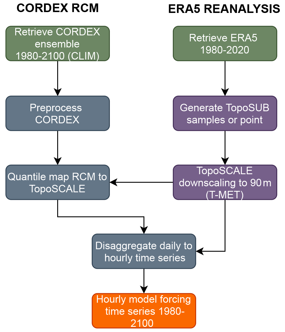
Figure 1 Schematic overview of the main TopoCLIM processes and the experimental setup used in this study.

2.2 Preprocessing

The CORDEX data download is achieved using a custom tool built around the ESGF Python client. This is not a trivial task due to the large data volumes involved and the variable uptimes of data nodes. All preprocessing of raw CORDEX data (Fig. 1) – concatenating NetCDF time series, extracting the region of interest, and regridding from rotated pole projections – is accomplished using standard tools from the Climate Data Operators (CDO) suite. The CDO tools are called from the preprocessing module of TopoCLIM and are not used as stand-alone command line tools – enhancing the ease of use and reproducibility of the processing pipeline. As downloads are done by variable, it is possible that the full set of required forcing variables may not be available for a given CORDEX model chain. If this is the case, the model chain is excluded from any further processing.

Climate model calendars are often simplified for numerical reasons and are inherited from the parent GCM. These need to be correctly handled to produce comparable time series. Three calendars exist in the CORDEX data used here: “360 d” (every month is 30 d long), “365 d” (no leap year), and “standard” (complete Gregorian calendar). We convert all calendars to “standard” by linearly scaling dates to the standard Gregorian calendar and then gap-filling missing data by linear interpolation.

For example, during the conversion from a “360 d” to a “standard” calendar, the output from linear scaling will result in a 365 d time series (except for a leap year) and will be missing the following dates: 31 January, 31 March, 1 June, 31 July, 30 September, and 30 November. In a second step, these dates are gap-filled using linear interpolation.

2.3 Spatial downscaling of reanalysis data

ERA5 reanalysis “observations” are downscaled using the TopoSCALE scheme (Fiddes and Gruber, 2014) for use as the reference data in the bias correction. We acknowledge that reanalyses are not true observations (Parker, 2016); yet, by assimilating an extensive set of observations into a numerical weather prediction (NWP) model, reanalyses are often considered to give the best possible view of the global climate (Dee et al., 2014). TopoSCALE performs a 3D interpolation of atmospheric fields available on pressure levels (to account for time-varying lapse rates) and a topographic correction of radiative fluxes. The latter includes a cosine correction of incident direct short-wave radiation on a slope, an adjustment of diffuse short-wave and long-wave radiation by the sky view factor, and an elevation correction of both long-wave and direct short-wave radiation. It has been extensively tested in various geographical regions and applications, e.g. permafrost in the European Alps (Fiddes et al., 2015), permafrost in the North Atlantic region (Westermann et al., 2015), Northern Hemisphere permafrost (Obu et al., 2019), Antarctic permafrost (Obu et al., 2020), Arctic snow cover (Aalstad et al., 2018), Arctic climate change (Schuler and Østby, 2020), and Alpine snow cover (Fiddes et al., 2019). This approach enables us to provide a climate length pseudo-observation time series globally while accounting for the main topographic effects on atmospheric forcing. We call this product T-MET throughout the text. It should be noted that this serves as our reference throughout the paper. A detailed validation and quantification of the uncertainty of the TopoSCALE method is given in Fiddes and Gruber (2014) and is therefore not repeated here. We do, however, compare our results to the station data variables of air temperature and snow depth across the IMIS network.

2.4 Quantile mapping

Bias correction through quantile mapping $Q:x\to x^{\star }$ is achieved as follows (Panofsky and Brier, 1968):

$$\begin{array}{}\text{(1)}& x^{\star }=Q\left(x\right)=F_{\mathrm{o}}^{-\mathrm{1}}\left[F_{\mathrm{m}}\left(x\right)\right],\end{array}$$

where the debiased output variable x^⋆ is obtained by applying the quantile mapping function Q to the biased input variable x. This function is generally formed through the composition of the modelled cumulative distribution function (F_m) and the inverse of the observed cumulative distribution function (F_o). In our case, F_o is obtained from the pseudo-observations in the form of downscaled ERA5 data, while F_m is generated from the CORDEX output that we want to bias correct.

We use the R package qmap for this purpose (Gudmundsson, 2016; Gudmundsson et al., 2012). Gudmundsson et al. (2012) compared different implementations of QM for daily precipitation data and found that a nonparametric empirical approach (as implemented in the cited package) outperforms implementations relying on theoretical distributional assumptions. While quantile mapping ensures that quantile biases are corrected in the CDF, it does not account for seasonally varying bias. It is therefore well suited to air temperatures for which we can be reasonably sure that winters are cold and summers hot, at least in mid- to high latitudes. However, with precipitation, the intra-annual distribution can be biased while the CDF may look reasonable (e.g. the wet and dry season timings could be shifted). We address this with a two-step approach called QM_MONTH. We split the data into 12 temporal subsets corresponding to the months of the calendar year and run the QM algorithm on each subset, computing QM parameters separately for each month. These are applied throughout the historical and climate time series at the appropriate months. Similar approaches have been used successfully in other studies, e.g. Hanzer et al. (2018). Quantile mapping is performed on a subset of data for the period 1980–1995 to allow an evaluation to be performed for the time period 1996–2006. It should be noted that these periods are constraints imposed by the datasets used in this study and can be changed in other applications of the method.

While the variables are bias corrected independently, they are corrected towards a physically consistent dataset in the form of downscaled ERA5 data. We argue that the method does not produce physically inconsistent results, despite being univariate. Validation performed for the current climate also supports this claim (Tables 3–5).

2.5 Temporal downscaling of climate time series

The final step in preparing the climate forcing is a temporal disaggregation to generate the required sub-daily fields. Original hourly-resolution T-MET data are used to temporally disaggregate the downscaled (quantile mapped) daily climate time series. The Melodist package is used for this purpose (Förster et al., 2016). This disaggregates daily data based on observed sub-daily distributions. It should be noted that this assumes that sub-daily distributions are stationary in a future climate, which quite possibly may not be the case. However, there is likely to be a greater source of uncertainty in the ability of ERA5 to reproduce short-timescale local weather patterns that require convection-resolving model resolutions (Liu et al., 2017) and appropriate physics.

Variables are disaggregated with the Melodist methods listed in Table 1 (Förster et al., 2016). Melodist does not however, provide methods for air pressure or long-wave radiation; these are handled with the following procedure. Taking advantage of the relationship between incoming long-wave radiation (L^↓) and the air temperature (T_a),

$$\begin{array}{}\text{(2)}& L^{\downarrow }=\mathit{ϵ}\times \mathit{\sigma }\times T_{\mathrm{a}}^{\mathrm{4}},\end{array}$$

where σ is the Stefan–Boltzmann constant (5.67×10⁻⁸ W m⁻² K⁻⁴), we diagnosed the daily all-sky emissivity (ϵ). We then used ϵ as a daily scaling factor to convert the disaggregated T_a into L^↓. This procedure therefore assumes a constant ϵ with a sub-daily time step (which, of course, will not normally be true), yet it ensures that L^↓ scales correctly with T_a. Therefore, higher T_a leads to higher L^↓ values and vice versa. Air pressure is simply linearly interpolated to the sub-daily time step.

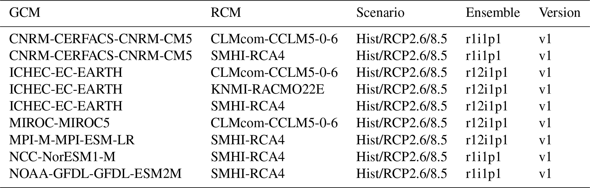
Table 1 CORDEX variables used in this study, together with the Climate and Forecast Conventions (CF) standard names.

3 Study region and data

3.1 Model domain

We consider two scales in this study: (a) point scale (meteorological stations: Weissfluhjoch and the IMIS network) and (b) regional (Swiss Alps), in order to illustrate typical applications of the scheme. A map of the study region and the locations of the stations we used is given in Fig. 2.

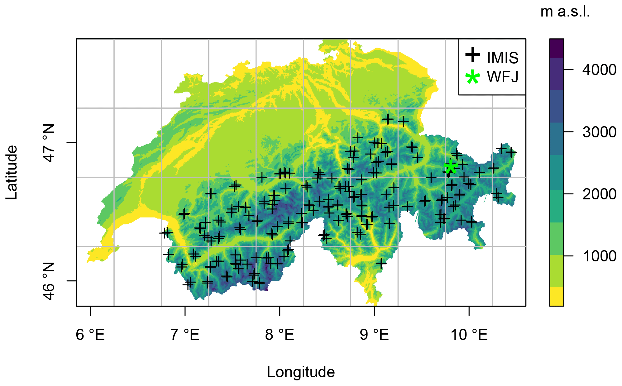
Figure 2 Study domain map with CORDEX EUR-44 grid (44 km) overlaid. IMIS stations and the Weissfluhjoch site (WFJ) are indicated.

3.2 Climate data

The basic forcing comes from the product with a nominal resolution of 44 km from the CORDEX EUR-44 regional climate model project (Jacob et al., 2014). The 44 km product was chosen over the 22 km product as it had many more model chains available. The EURO domain also has an 11 km product, but this is not available for all CORDEX regions and is therefore not fit for the purpose of this study, which aims to be a globally applicable method based on datasets that are available worldwide. Data were retrieved from the ESGF using an API and automated Python-based tool developed in this study. This is an important step as the number of file downloads is large, with dimensions of $\text{models}\times \text{variables}\times \text{scenarios}\times \text{time periods}$. The fact that the ESGF consists of a distributed set of data nodes with variable uptimes further complicates the download process. We use daily data to force the scheme and retrieve historical data plus projections from two climate change scenarios, RCP2.6 (a very stringent pathway; RCP2.6 requires that CO₂ emissions start declining by 2020 and go to zero by 2100) and RCP8.5 (where emissions continue to rise throughout the 21st century). A full description of CORDEX variables is given in Table 1, and the model chains used are shown in Table 2. Daily data were chosen for the method (therefore requiring a temporal disaggregation step), as a limited number of model chains are available at sub-daily resolutions. This is particularly the case outside of the EURO domain, where use cases for this method are envisaged. A higher number of model chains increases confidence in our results by improving the quantification of inter-model variability.

Table 2 CORDEX model chains used in this study.

3.3 Reanalysis data

We use ECWMF's latest reanalysis product, ERA5 (Hersbach et al., 2020), which uses version 41r2 of IFS – the ECMWF NWP model. ERA5 represents an evolution over its predecessor, ERA-Interim, as it increases the model's spatial resolution to 0.25^∘, the temporal resolution to hourly, and the vertical model levels to 137 (37 pressure levels are stored). These reanalysis data are downscaled for the purpose of bias correction using the TopoSCALE scheme (Fiddes and Gruber, 2014), as described above (see “Methods”).

3.4 Topography

NASA's SRTM-3 90 m digital elevation model (DEM) is used as a topographical surface for TopoSCALE downscaling routines. Slope, aspect, and sky-view factor (the portion of the sky hemisphere that is visible for a given DEM pixel) are derived (Dozier and Frew, 1990).

A higher-resolution DEM may also be used but is unlikely to add value, as processes such as wind transport that operate on these scales are not included in the model (Mott et al., 2018). However, it should be noted that avalanching off steep slopes is accounted for by removing snow linearly above a slope threshold (Fiddes et al., 2015). Importantly in our scheme, a higher resolution does not necessarily increase the runtime either in point mode (trivially) or in spatial mode, where the runtime in the main programme modules is related to the number of TopoSUB clusters. Additionally, the scheme is designed to scale well by generating cluster forcings through array computations.

4 Simulation setup and evaluation

4.1 Simulation and maps

We use the Factorial Snow Model (FSM) (Essery, 2015) to simulate the snow cover and TopoSUB (Fiddes and Gruber, 2012) to spatialize the results onto a 2D map. FSM is a multi-physics ensemble model; however, in this study, we always use configuration 31, which is the most complex version of the model, where all five parameterizations are switched on. TopoSUB is a topographic sampling scheme that reduces distributed modelling problems that explicitly model individual pixels to a lumped model several orders of magnitude smaller while considering the full range of topographic heterogeneity that exists. For example, a 100 m grid over a 25 km × 25 km domain would have 62 500 pixels, which would each represent a model simulation in a fully distributed setup of many surface models. TopoSUB would reduce this to 100–200 samples, each representing a single model run, corresponding to a reduction in computation of around 3 orders of magnitude. It achieves this by using a k-means clustering algorithm (MacQueen, 1967) to perform a multidimensional classification on terrain parameters in the model domain, resulting in so-called TopoSUB clusters consisting of pixels with similar terrain parameters.

The predictors used in the clustering algorithm are elevation, slope, aspect, and sky-view factor. In this way, it is possible to produce high-resolution maps (e.g. DEM resolution) over large (regional) modelling domains while explicitly including important drivers of surface–atmosphere processes. The scheme is implemented on an HPC cluster for efficiency in an “embarrassingly parallel” sense, i.e. no communication is required between compute nodes. Typical setups use 100 nodes with runtimes measured in minutes for 1980–2100 runs, for example to produce the results given in Fig. 7. The scheme also has a desktop mode that typically utilizes eight cores, and typical runs will require a few hours. These indicative numbers are provided merely to give the reader an order-of-magnitude idea of how frugal this scheme is in terms of computation resources compared to dynamical downscaling.

4.2 Treatment of glaciers

Glacier zones are typically masked in studies of seasonal snow unless a glacier layer is explicitly accounted for in the model. In this study, however, we wanted to highlight and track changes in the glacier accumulation zones. These zones are areas where the annual surface mass balance is positive, leading to the formation or growth of glaciers. With our framework, we are able to identify such zones, as we are able to model areas with perennial snow cover with FSM, and these give a good indication of glacier accumulation zones under a given climate. However, we ignore glacier dynamics, so we are not able to adequately map the spatio-temporal evolution of glaciers.

4.3 Evaluation

Predictive methods must, by definition, be evaluated on data independent from that used for calibration in order to correctly evaluate how applicable a model is beyond the data space within which it was developed. Further, highly adaptable methods, such as the nonparametric techniques used in this study, are prone to overfitting. These issues are avoided in this study as we perform an independent evaluation using station data from the IMIS station network, whereas calibration, or in this case downscaling, is performed using downscaled ERA5 fields. Note that none of the meteorological fields of the IMIS stations were assimilated during the production of ERA5. Snow depth results are evaluated using automatic snow depth measurements obtained by sonic ranger (Campbell Scientific SR50), which are available from the Intercantonal Measurement and Information System (IMIS) station network at 30 min intervals. This is a high-elevation station network that forms the backbone of the national avalanche service in Switzerland.

The analysis in this study is organized as follows. The reference period is defined as 1981–2010, and future scenarios are analysed for climate periods 2031–2060 and 2070–2100. We assess the downscaling of all meteorological fields at the Weissfluhjoch IMIS station (Fig. 3), which has the full suite of variables produced, as compared to standard IMIS stations, which lack a full radiation balance. Here, we additionally test the performance of the scheme at point scale (Figs. 4 and 5). We further assess air temperature and snow depth (as a proxy for precipitation) using the entire IMIS network (Fig. 6). We do not assess precipitation directly, as year-round datasets are not available from the IMIS network due to unheated gauges, and snow depth is often considered a more robust variable to measure at high elevation. After this, we provide results from using the scheme at various spatial scales (Figs. 6–8).

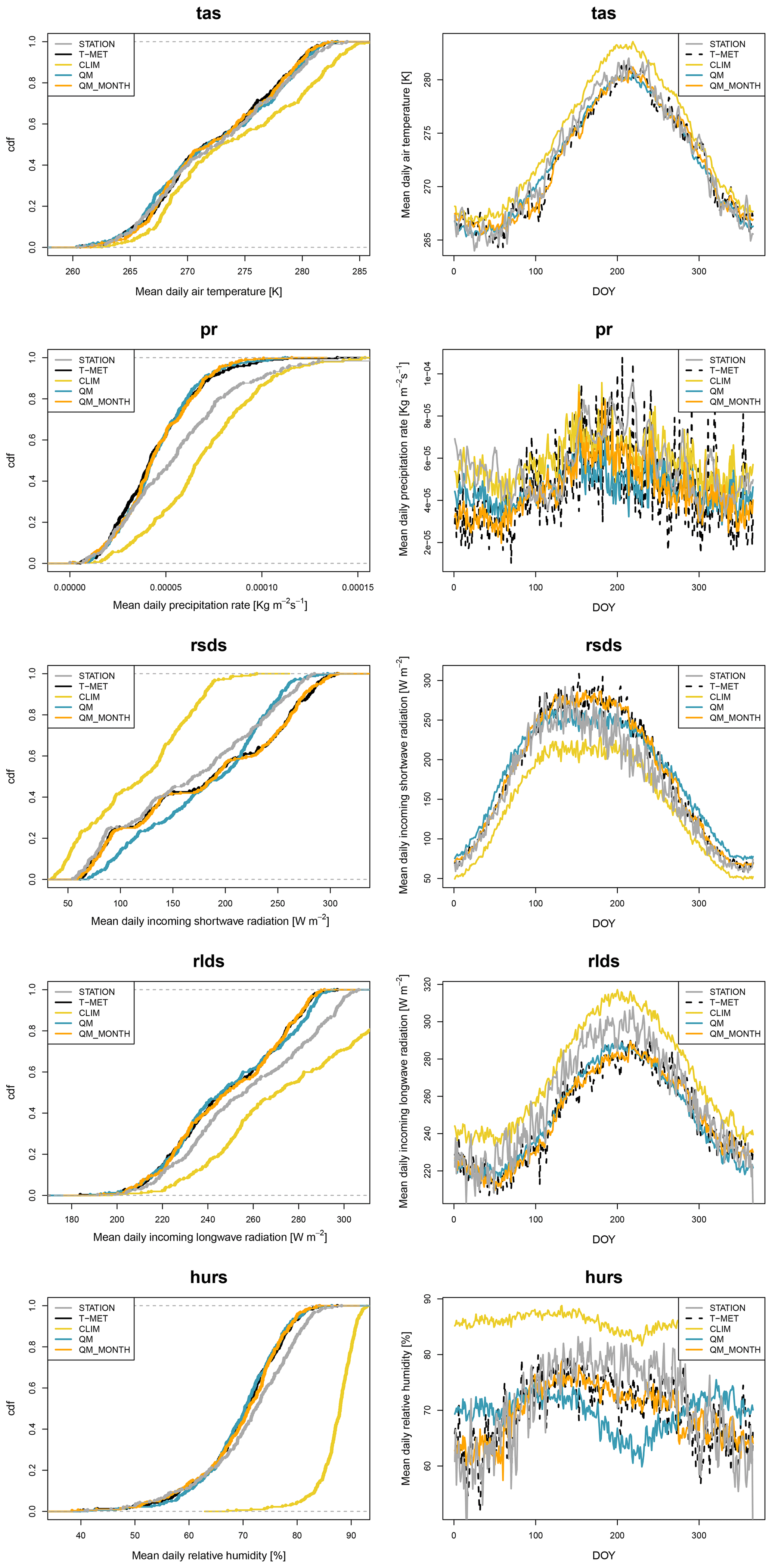
Figure 3 Evaluation of the quantile mapping routine at the Weissfluhjoch station in the standard-mode single-parameter set QM and the seasonally varying parameter set QM_MONTH. CLIM is the uncorrected CORDEX dataset. STATION is the set of measurements from the Weissfluhjoch station. T-MET is the downscaled ERA5 data obtained using TopoSCALE. Shown are the cumulative density function over the period 1981–2010 (left panel) and seasonal distribution given as the average by day of year (DOY) for the same period (right panel).

5 Results and discussion

5.1 Evaluation at the Weissfluhjoch station

Figure 3 and Tables 3 and 4 (statistics) show an evaluation of the scheme at the WFJ station both as a cumulative distribution function (left column) and a day-of-year (DOY) plot that averages all values in the time series for a given DOY (right column). Here, we compare the gridbox CORDEX ensemble mean (CLIM), a single parameter set quantile map run (QM), and a monthly parameter set quantile map run (QM_MONTH) to T-MET and station measurements. This comparison is done over the period 1996–2006, which corresponds to the overlapping time frames of CORDEX-HIST, T-MET, and station data, and also – importantly – does not include the period over which quantile mapping is run (1980–1995). We perform two sets of comparisons. The first is with T-MET as a reference, as this is the target of the quantile mapping (Table 3). This shows how the scheme behaves, particularly in terms of the different QM and QM_MONTH implementations (Table 3). In the second, we compare results directly to the measurements at the station to get a global look at how the scheme performs (Table 4). Of course, this is then subject to residual error in the TopoSCALE downscaling scheme that produces T-MET (Table 5) and therefore must be interpreted carefully.

Table 3 Statistics from the evaluation shown in Fig. 3. Correlation (R), root mean squared error (RMSE), and percentage bias (PBIAS) are given relative to the downscaled ERA5 data T-MET.

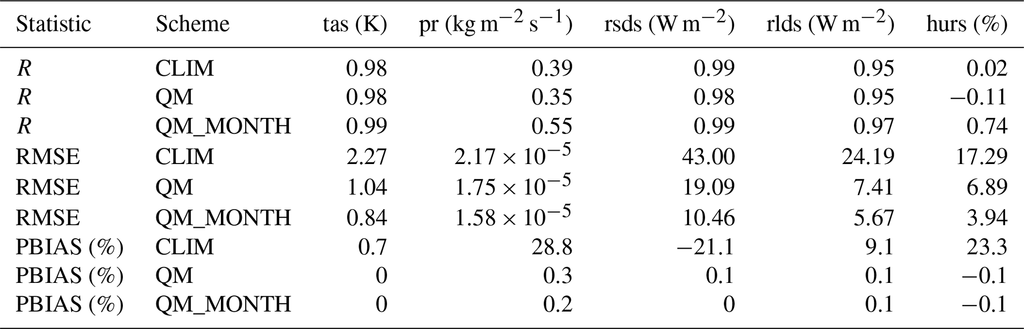
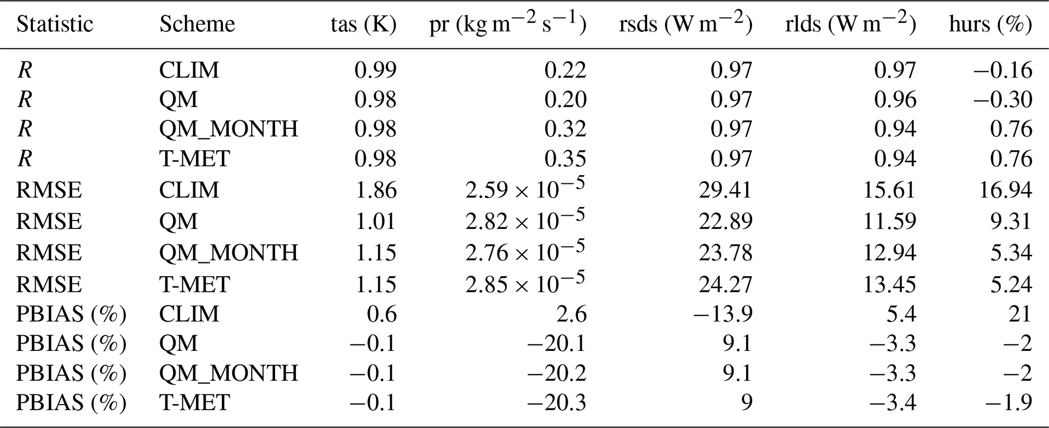
Table 4 Statistics from the evaluation shown in Fig. 4. Correlation (R), root mean squared error (RMSE), and percentage bias (PBIAS) are given relative to station measurements at Weissfluhjoch (STATION).

With respect to the target T-MET (Fig. 3, Table 3), percentage bias and RMSE are generally strongly decreased by the scheme in the standard QM mode and further by the QM_MONTH variant, especially where there is a time-varying bias signal (e.g. short-wave radiation).

With respect to station measurements (Table 4), we see an overall improvement in statistics using the scheme, but this is not always reflected in an improvement in statistics between QM and QM_MONTH, as there is residual error in the downscaled T-MET with respect to the station measurements. The strongest improvements are in variables that are downscaled according to model pressure levels in the TopoSCALE scheme (air temperature and relative humidity). Precipitation is the only parameter for which we do not see an improvement in the scheme with respect to the measurements, but this is expected due to the high uncertainty in precipitation and the fact that this is not addressed by the base TopoSCALE downscaling. This point is further discussed below in Sect. 5.4.

Figure 4 shows a typical point-scale application that generates a forcing time series, in this case for air temperature. The effect of the bias correction is shown, with a clear improvement observed with respect to T-MET. Figure 5 gives a point-scale example of snow depth evolution at WFJ. Available snow depth observations from WFJ show good agreement with both the historical period and the first decade of the RCP runs in terms of lying within the model ensemble. It should be stressed that a quantitative comparison with individual years cannot be made, as the variability in CORDEX (and climate models more generally) is not expected to be perfectly synchronized with the observed variability at temporal resolutions of years to a decade. Note that the stable/rising snow depth by the end of the century under RCP2.6 is correlated to the stabilized mid-century temperatures shown in Fig. 4.

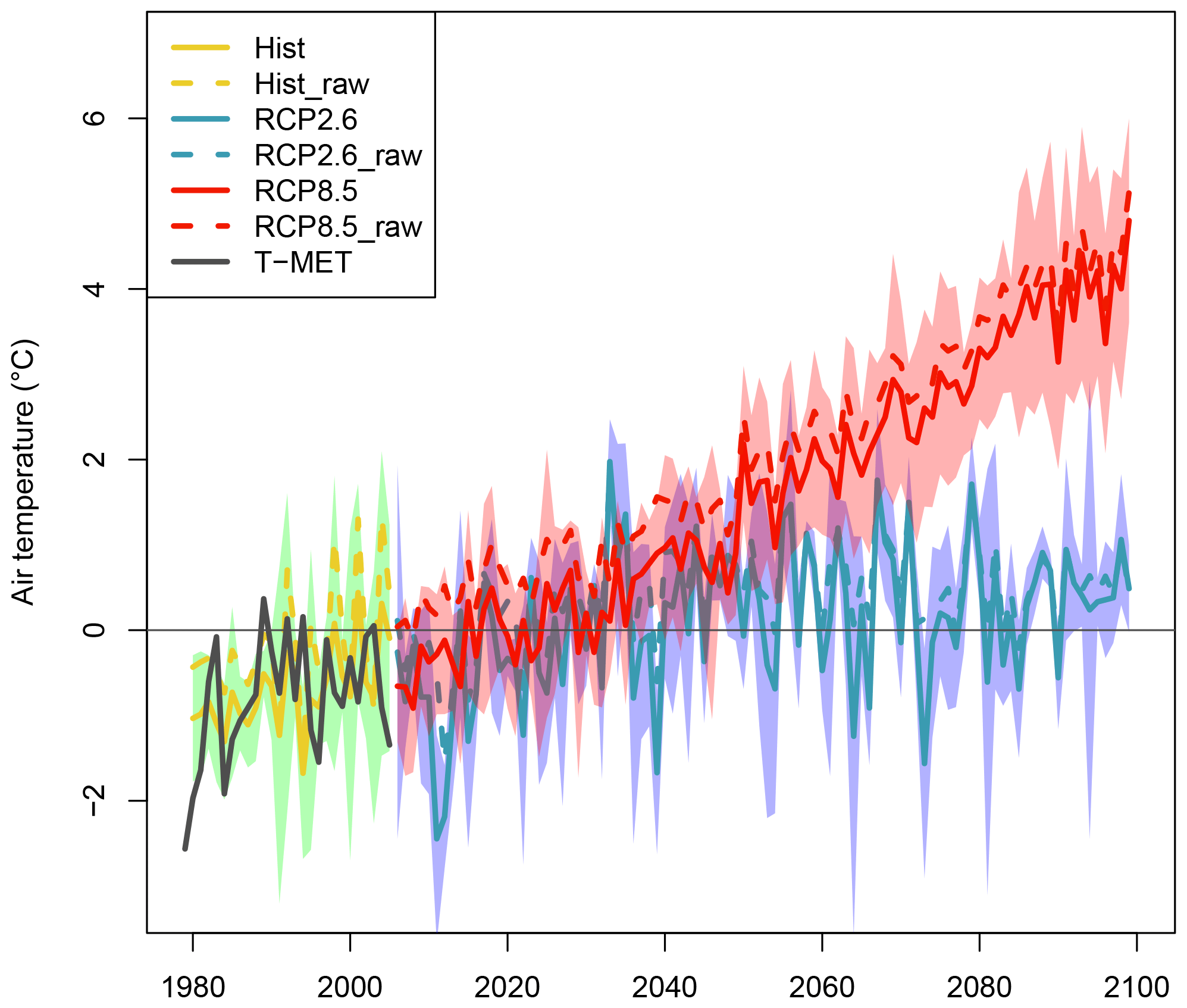
Figure 4 A point-scale TopoCLIM product: the mean annual near-surface air temperature at the Weissfluhjoch (2540 m a.s.l.), showing corrected historical, RCP2.6, and RCP8.5 time series. T-MET and uncorrected CORDEX data are also shown for comparison. The coloured envelopes indicate the model spread and the ensemble mean is given by the bold line. The zero degree isotherm is given by the horizontal line.

Figure 5 An example of a point-scale TopoCLIM product: the mean annual snow depth (m) ensemble at the Weissfluhjoch station (2540 m a.s.l.) for historical and future RCP scenarios. Observations from Weissfluhjoch are given in black for a qualitative comparison. Ensemble means are indicated by solid lines, and the long-term average over the plotted historical period (1981–2010) is given by the horizontal line. Observations lie within the ensemble spread, indicating that the bias correction method works satisfactorily. It should be stressed that we do not attempt a quantitative comparison here, as the variability of CORDEX (and climate models more generally) is not expected to be perfectly synchronized with the observed variability. Nonetheless, this representation usefully shows the inter-annual variability present in both the model and the observations instead of simply showing decadal means.

5.2 Evaluation for the IMIS network

Figure 6 gives the evolution of snow depth averaged across the IMIS network in terms of mean DOWY (day of water year) snow depth, starting at 1 September. IMIS station measurements are given as reference, but it should be noted that the time period covered by each station is variable within the period 1996–2018. The shortest station record is 10 years. These are compared to the T-MET snow depth by only using the days present in the IMIS dataset. At this synoptic spatial and temporal scale there is good agreement, with low bias and RMSE scores and high correlation (Table 4). The evolution of snow depth is given for future climate scenarios and two future periods. By mid-century, with respect to the reference CORDEX historical period (CORDEX-HIST), a reduction in peak snow depth of around 20 cm is seen under RCP2.6, and a further 25 cm is seen under RCP8.5. Peak snow depth occurs around 30–40 d earlier. In RCP2.6, the snow depth has not further deteriorated by late century; in fact, it shows signs of a possible recovery, with the peak snow depth moving towards that of the CORDEX-HIST period. RCP8.5, however, gives a strong further reduction in peak snow depth of around 1 m with respect to CORDEX-HIST. The comparison between CORDEX-HIST (1980–2006) and T-MET/IMIS (1996–2018) is useful but should be treated with caution due to the only partially overlapping periods (defined by the availability of station measurements). The CORDEX-HIST period has a higher peak snow depth and a later snow melt-out date, which could be due to less climate change, as it represents an earlier period than IMIS and T-MET.

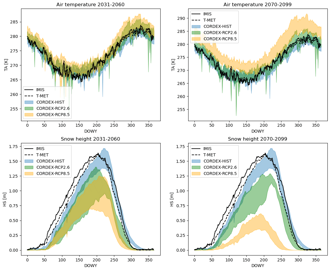
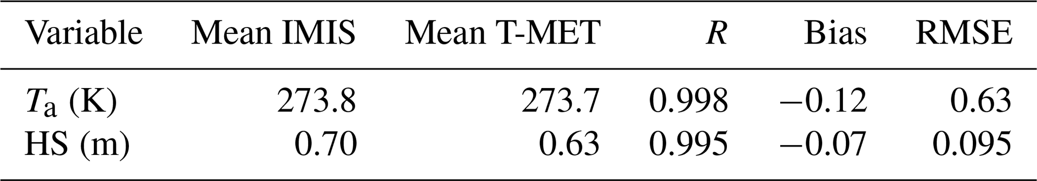
Figure 6 Large-scale evaluation of the scheme at all IMIS station locations. Network mean air temperature and snow depth across all IMIS stations (IMIS) are compared to the same data generated by the TopoSCALE downscaling of ERA5 (T-MET) and TopoCLIM-downscaled CORDEX data for the historical period (1981–2010) and scenarios RCP2.6 and RCP8.5 for near-future (2031–2060) and far-future (2070–2099) periods for each day of water year (DOWY), starting at 1 September. The full width of the model ensemble is represented by the shading. Note that T-MET and IMIS have the same time frame (which varies by station between 1996 and 2020) and are therefore directly comparable (see Table 5), but this only partially overlaps with the CORDEX historical period and is therefore intended for visual comparison only.

Table 5 Statistics from the evaluation comparing T-MET results with IMIS station data for the historical period, as shown in Fig. 6.

5.3 Impacts of climate change on Alpine snow cover across Switzerland

As an example of the application of the full model pipeline, the results in Fig. 7 were generated by feeding model results (TopoCLIM/FSM) to the TopoSUB spatial framework to generate transiently modelled snow-depth maps at 100 m resolution. The ensemble mean is used in each scenario/time-period plot. We highlight again that when we using this simple approach, we implicitly model climate-viable glacier accumulation zones, where the snowpack does not melt out by the end of summer. Mid-century results for RCP2.6 and RCP8.5 are comparable except for lower-elevation areas such as the Jura mountains in the far west of Switzerland. By late century, the difference is large (as also seen in Fig. 6), with a strong increase in snowline elevation and a reduction of snow depth, even at high elevations. Glacier accumulation zones remain only in the high Valais (Mattertal) and Bernese Oberland around the current accumulation zone of the Aletsch Glacier. Figure 8 provides a more quantitative picture of snow cover–elevation dynamics. This hypsometric plot summarizes the pixels of Fig. 7 by showing the mean and standard deviation of the snow depth at each 50 m elevation band across the entire domain for three time periods and scenarios RCP2.6 and RCP8.5. As expected, a strong decrease in snow depth is seen at all elevations under RCP8.5. A slightly different story unfolds under RCP2.6, with snow depth reducing up to mid-century but then increasing at high elevations (above 3500 $\mathrm{m}\mathrm{a}.\mathrm{s}.\mathrm{l}.$) by the end of the century – this is a consistent finding throughout this study and reflects the results of Figs. 5, 6, and 7. It can be partially explained by the stabilization of air temperatures by mid-century (Fig. 4) together with increased precipitation in the Alpine region (Jacob et al., 2014; Smiatek et al., 2016).

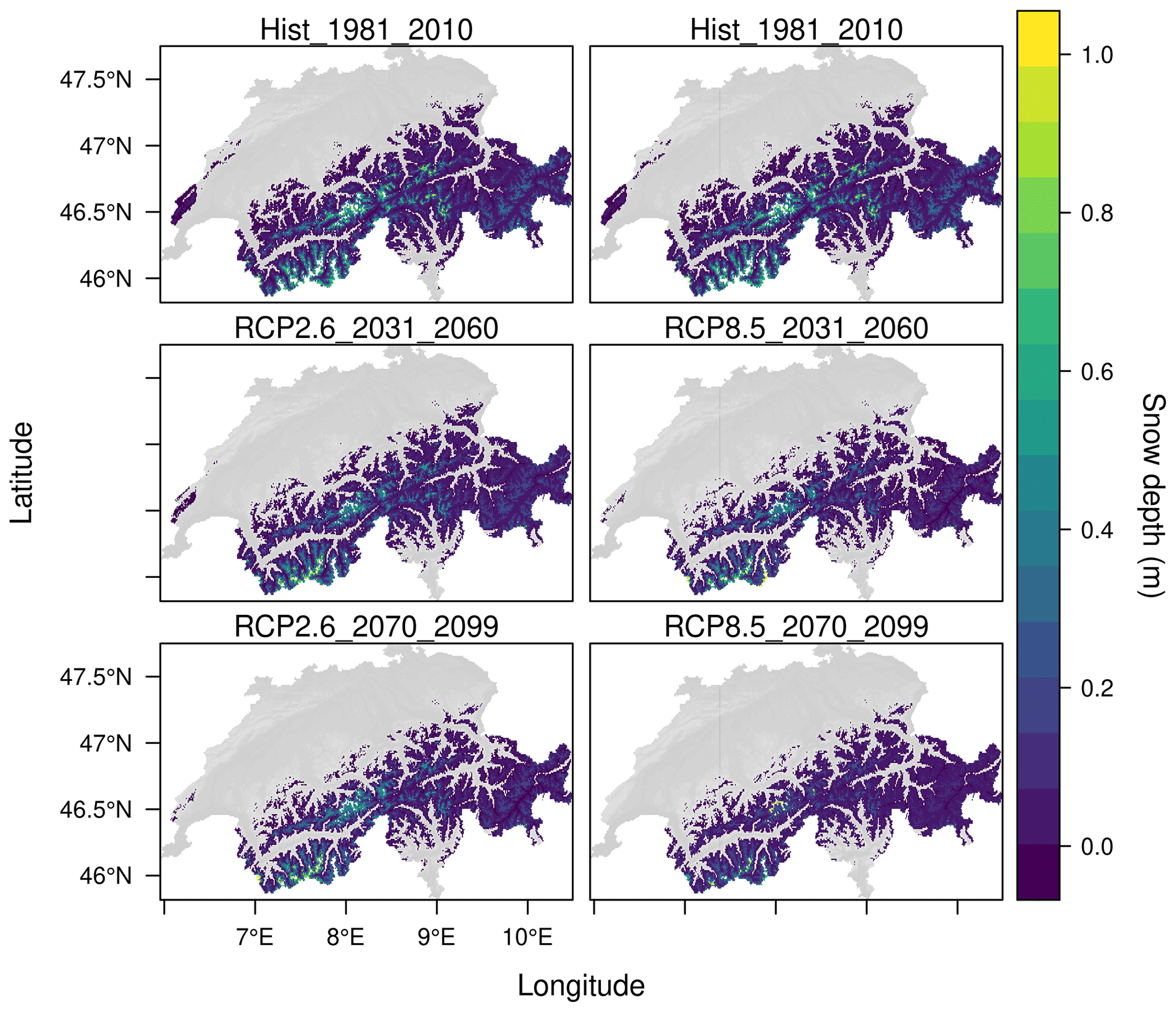
Figure 7 Example TopoCLIM forced climate-change maps: mean snow depth (m) for RCP2.6 and RCP8.5 (columns) during the time periods 1981–2010, 2031–2060, and 2070–2099 (rows). Perennial snowpack (i.e. the snow does not melt on an annual cycle) is masked out (white regions) and assumed to represent climatological glacier accumulation zones.

An interesting observation about this figure is that, in all time periods and scenarios, snow depth is limited at low elevation by temperature and at high elevation by terrain, which tends to be steeper and therefore permits lower accumulations due to avalanching (permitted by the model, as discussed in Sect. 3.4). A final point of note regarding this figure is the truncation level indicating the accumulation zone elevation, which is approximately 4000 m for HIST. Above this level, seasonal snow is not possible, as it will not melt before the following winter season or the ground is too steep for snow accumulation. This upper limit for seasonal snow rises to around 4500 $\mathrm{m}\mathrm{a}.\mathrm{s}.\mathrm{l}.$ over the 21st century – well above former glaciated surfaces. An implication of this for water resources is that, while we will lose a large quantity of glacier accumulation zones during the 21st century irrespective of the scenario, it is unlikely that we will lose seasonal snow-water resources at those elevations.

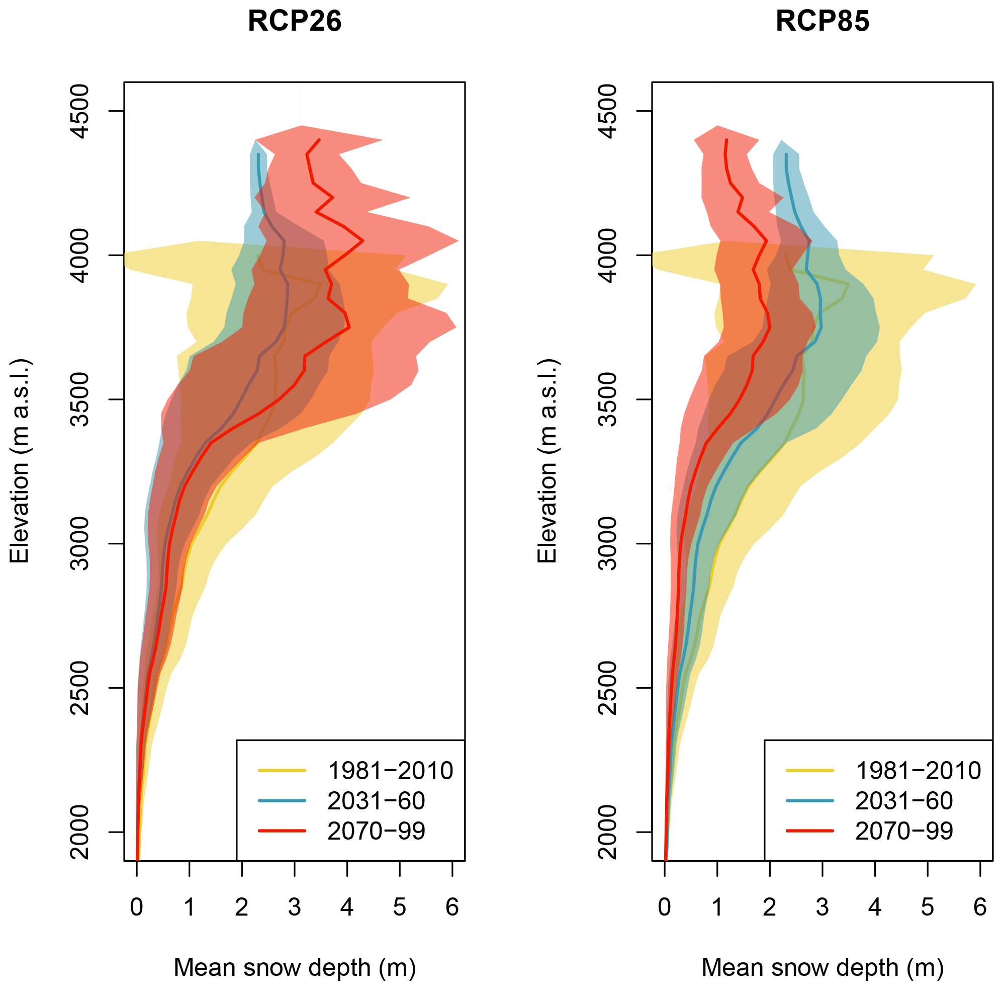
Figure 8 Hypsometry of snow depth over the Swiss Alps for RCP2.6 and RCP8.5 for the periods 1981–2010, 2031–2060, and 2070–2099. These data are derived from the ensemble mean, with shading showing ±1 standard deviation of the values in each elevation band. The elevation limit in each time period corresponds to the threshold between seasonal and nonseasonal snow, or glacier accumulation zones. This demonstrates the rising equilibrium-line altitude of glaciers over the 21st century in all RCPs and the extension of seasonal snow into the former glacier zones.

Several previous studies have investigated the impacts of climate change upon Alpine snow cover (e.g. Verfaillie et al., 2018; Steger et al., 2012; Marty et al., 2017; Frei et al., 2018; Bender et al., 2020), but a direct comparison is often problematic due to the model resolution, analysis period, parent climate models, and/or emissions scenarios used. This highlights the importance of model intercomparison studies whereby these important variables that control model results can be standardized. Comparison to the previous works cited highlights the contribution of this study, in that most were conducted at an RCM resolution of 25–12 km (e.g. Steger et al., 2012; Frei et al., 2018) or the local scale (e.g. Verfaillie et al., 2018; Bender et al., 2020) or are reliant on in situ data (e.g. Marty et al., 2017; Bender et al., 2020). In this study, we demonstrate a method that generates results over large modelling domains at the hillslope scale, a scale which is extremely important in regulating the stores and fluxes of water, energy, and carbon (e.g. Fan et al., 2019) and is therefore critical to modelling snow cover in mountainous terrain. Additionally, this approach does not rely on in situ data and is therefore appropriate for data-scarce regions.

5.4 Forcing uncertainty

The largest source of uncertainty in the scheme is the reanalysis forcing from ERA5. Both quantile mapping and disaggregation of fields to sub-daily time steps are inherently constrained by the distribution of ERA5 fields. While ERA5 provides hourly data and therefore resolves the diurnal cycle, it remains a 0.25^∘ model with a correspondingly smooth topographical surface representation and parameterization of physical processes that occur on shorter length scales. Typical examples are convective precipitation and cold air pooling in valley bottoms (Cao et al., 2017; Liu et al., 2017) and orographic enhancement of precipitation and wind fields (Gerber et al., 2018; Mott et al., 2018; Gutmann et al., 2016). As the density of observations that are assimilated in reanalyses varies globally, we expect the performance of the TopoCLIM model pipeline to be a function of how well constrained ERA5 is in any given location. A full analysis and discussion of TopoSCALE uncertainties is given by Fiddes and Gruber (2014) and to some extent in Fiddes et al. (2019). The most uncertain variable is precipitation, which is clearly a critical point for snow modelling studies. We do, however, show that there are no large-scale biases in the precipitation field, at least in our snow depth comparison across the IMIS network. We have shown in previous studies that variables that drive the energy balance (air temperature, incoming short-wave radiation, incoming long-wave radiation) are downscaled with good skill by TopoSCALE. One method we have explored to reduce (and quantify) meteorological forcing uncertainty and precipitation uncertainty in particular is Bayesian data assimilation of globally available satellite products using a particle batch smoother, and this has shown promising results (Fiddes et al., 2019; Alonso-González et al., 2020). The coupling of this scheme with TopoCLIM will be the subject of subsequent work.

5.5 Evaluation uncertainty

Our station measurements are characterized by considerable uncertainties – a problem that is particularly acute for precipitation-related fields such as snow depth. Therefore, to some extent, we have a chicken and egg scenario when it comes to model validation, in that it is hard to untangle the origin of apparent errors. For example, stations tend to be situated in sheltered flat-to-concave topography, where we would expect there to be a considerable preferential deposition (Lehning et al., 2008) from surrounding windblown slopes and ridge lines (Grünewald and Lehning, 2015). In general, therefore, we would expect stations to be positively biased with respect to large-scale precipitation fluxes. Additionally, certain stations will be exposed to very local climatic effects that are not represented in the large-scale 0.25^∘-resolution ERA5 forcing. Examples of such local effects include wind funnelling leading to scouring, enhanced Foehn effects, and local orographic enhancement.

5.6 Snow model uncertainty

The snow model used in this study, FSM, is an intermediate-complexity physically based model, and we do not expect it to perform as well with respect to snow densification as a more complex snow physics model such as SNOWPACK (Lehning et al., 2002; Wever et al., 2015). This can introduce uncertainty when using snow depth as a validation parameter. However, it should be noted that there is active discussion about snow model complexity and how this does not necessarily lead to improved performance (see Magnusson et al., 2015). Snow water equivalent is a simpler modelling objective but a much harder measurement objective, so few sites are available, particularly with good coverage at regional scales, thereby limiting its applicability for large-scale evaluations.

6 Conclusions

In this study, we have developed and tested a new scheme for downscaling regional climate projections that is specifically designed to provide hillslope-scale forcings for impact models. We take advantage of the now globally available CORDEX RCM data to develop a method with global scope. The scheme adheres to the approach of TopoSCALE, upon which it builds: modelling tools that bridge the gap between relatively simple empirical approaches and full dynamical models that require extensive computing resources. It can be run in both desktop and cluster environments. The target application of this scheme is impact modelling in complex terrain where significant atmosphere–surface interactions need to be considered. A particular application is in remote areas where ground data may either not be present at all or not available for the duration of a climate normal period, meaning that traditional ESD methods are problematic to use. Another strength of this approach is that it produces continuous time series, such that it permits transient simulations, in contrast to other parsimonious methods such as the delta-change approach. This is an important point for domains such as soil, ground ice, or glaciers, where surface forcings drive processes over decadal timescales.

This framework is adaptable to any kind of meteorological input data (both the reference data and the future/past period). Here, we have given an example with the reference based on downscaling ERA5, but it could equally be generated by downscaling other reanalyses such as MERRA or outputs from regional models such as WRF, COSMO, or ICAR. The method would also be applicable to other future projections such as those from CMIP6 that are coming online now. Exploring all these possibilities is beyond the scope of this paper, but it is useful to emphasize the potential applications of this framework. Another aspect to highlight is that we are downscaling an ensemble of CORDEX outputs, which also gives us a better idea of the uncertainty in future climate projections and impacts on the snowpack (in this case). It should also be stated that other downscaling routines or bias correction approaches could be used as a framework. The modularity allows these options to be explored. The very efficient combination of steps presented in this paper provides a powerful way of rapidly obtaining hillslope-scale climate forcings anywhere on the globe.

As a final point, TopoCLIM can be used to bias correct any dataset that partly overlaps with the reference period. Thus, in addition to the future projections considered in this study, it would also be possible to use TopoCLIM to correct coarser-scale reanalysis data that stretch far back in time. A prime example would be ECMWF's 20th century reanalysis (ERA-20C), which spans 1900–2010 and thus partly overlaps with ERA5 (1950 to today), which is used to drive TopoSCALE to generate the reference data T-MET.